CREDIT, HOUSING COLLATERAL AND … housing collateral and consumption: evidence from the uk, japan and the us john v. duca research department working paper 1002 federal reserve bank

CREDIT, HOUSING COLLATERAL AND CONSUMPTION: EVIDENCE FROM THE UK, JAPAN AND THE US

JOHN V. DUCA

RESEARCH DEPARTMENT

WORKING PAPER 1002

Federal Reserve Bank of Dallas

Credit, Housing Collateral and Consumption:

Evidence from the UK, Japan and the US

Janine Aron, Department of Economics, University of Oxford, UK

John V. Duca, Federal Reserve Bank of Dallas, Southern Methodist University, US

John Muellbauer, Nuffield College, University of Oxford, UK

Keiko Murata, Tokyo Metropolitan University, Japan

Anthony Murphy, Hertford College, University of Oxford, UK

21 May 2010

Abstract: The consumption behaviour of UK, US and Japanese households is examined and compared using a modern Ando-Modigliani style consumption function. The models incorporate income growth expectations, income uncertainty, housing collateral and other credit effects. These models therefore capture important parts of the financial accelerator. The evidence is that credit availability for UK and US but not Japanese households has undergone large shifts since 1980. The average consumption-to-income ratio shifted up in the UK and US as mortgage down-payment constraints eased and as the collateral role of housing wealth was enhanced by financial innovations, such as home equity loans. The estimated housing collateral effect is roughly similar in the US and UK, while land prices in Japan still have a negative effect on consumer spending. Together with evidence for negative real interest rate effects in the UK and US and positive ones in Japan, this suggests important differences in the transmission of monetary and credit shocks between Japan and the US, UK and other credit-liberalized economies.

Keywords consumption, credit conditions, housing collateral and housing wealth JEL Codes E21, E32, E44, E51 *We thank Jessica Renier for research assistance. An earlier version was presented at the American Economic Association meetings and at Statistics Norway, in 2009, and we are grateful for comments received. The views expressed are those of the authors and do not necessarily reflect those of the Federal Reserve Bank of Dallas, or the Board of Governors of the Federal Reserve System. Any remaining errors are our own. Research support is acknowledged from the ESRC under “Improving Methods for Macro-econometric Modelling”, RES-000-23-0244.

1

1. Introduction

The global economic crisis of 2008-9 had its origins in a credit crisis, at the heart of which is

asymmetric information between lenders and borrowers, most simply the fear that lenders

have about the ability and willingness of borrowers to service debt. It is now generally

accepted that the household credit channel played an important part in the boom preceding

the crisis, as well as in accentuating the crisis with its origins in the sub-prime mortgage

market.

The multiple transmission channels of the original mortgage and housing crisis are

illustrated in Figure 1, which for visual simplicity omits the reverse transmission from lower

economic activity back to housing and mortgage markets, consumer spending, bank balance

sheets, other asset prices and credit spreads. Four main channels are illustrated: via

residential construction; via housing collateral and direct credit influences on consumption;

and via the lowered capital base of banks and other financial firms feeding into credit

standards and credit spreads, and more generally into the risk appetite of investors. This

articulates the down-phase of the financial accelerator. The same mechanisms operate in a

boom, albeit at a slower pace, where an initial expansion of credit availability, possibly due to

financial innovation and / or low global interest rates, tends to be amplified.

--- Figure 1 About Here ---

The financial accelerator is frequently neglected in the econometric models that, for

the last decade, have been popular with central banks and with main-stream macro

economists. Many dynamic stochastic general equilibrium (DSGE) modellers focused on

building macro models with rational expectations and micro-foundations that could generate

nominal rigidities by incorporating ‘New Keynesian’ frictions, primarily price stickiness and

adjustment costs. Practical modelling issues resulted in the widespread adoption of micro

foundations that too often ignored the asymmetric information revolution of the 1970s and

1980s. These models also neglected the information coming from the flow of funds and the

corresponding balance sheets, now receiving far more attention from central banks

(Gonzalez-Paramo, 2009, Eichner et al., 2010). In a recent speech, the Vice Chairman of the Federal Reserve, Donald Kohn (2008)

criticized such models:

1

“The recent experience indicates that we did not fully appreciate how financial

innovation interacted with the channels of credit to affect real economic activity--both as

credit and activity expanded and as they have contracted. In this regard, the macroeconomic

models that have been used by central banks to inform their monetary policy decisions are

clearly inadequate. These models incorporate few, if any, complex relationships among

financial institutions or the financial-accelerator effects and other credit interactions that are

now causing stresses in financial markets to spill over to the real economy. Rather, these

models abstract from institutional arrangements and focus on a few simple asset-arbitrage

relationships, leaving them incapable of explaining recent developments in both credit

volumes and risk premiums. Economists at central banks and in academia will need to devote

much effort to overcoming these deficiencies in coming years.”

No existing DSGE or other macro model fully captures the linkages and feedbacks

shown in Figure 1. This necessarily implies that the individual elements of such a model

require development without, initially at least, using a general equilibrium specification. The

two crucial equations are for house prices and consumer spending. We have modelled

elsewhere the critical role of shifts in credit supply in explaining house prices and of

extrapolative expectations in the overshooting of house prices1. In this paper, we present

estimates of consumption functions in the tradition of Modigliani and Brumberg (1954, 1980)

and Ando and Modigliani (1963) for three major economies, explicitly incorporating both

income expectations and credit channel influences. We show that, consistent with theory,

these credit channel effects differ across countries and over time. The estimated consumption

functions take full account of household balance sheet data, addressing important

measurement issues both for income and for wealth.

Early work in this area attributed much of the fall in the UK household saving ratio to

credit market liberalisation and the increase both in house prices and in the ‘spendability’ of

housing and perhaps other illiquid wealth (Muellbauer and Murphy, 1989, 1990)2. Further

research is summarized in Muellbauer and Lattimore (1995), which sets out the foundations

of a solved-out consumption function encompassing both classical life-cycle/permanent

income theory and credit channel features3.

1 Muellbauer and Murphy (1997), Cameron et al. (2006) and Duca et al. (2010a). 2 A different view contends that an exogenous shift in income growth expectations accounted for most of the fall in the saving ratio (King (1990) and Pagano (1990)). 3 Although this paper had a notable influence on the consumption function of the Federal Reserve’s FRB-US model and Brayton et al. (1997) devoted thorough attention to modelling expectations in FRB-US, the academic

2

This research has important implications for how the role of housing collateral in

consumption decisions can differ across countries and shift structurally over time due to

credit market liberalization. With imperfect capital markets, the price and availability of

borrowing are affected by agency costs that give rise to down-payment constraints in housing

markets. Research by Japelli and Pagano (1994), Engelhardt (1996) and others demonstrates

that mortgage down-payment constraints generate an economically significant motive to save.

In countries with limited access to consumer and mortgage credit, such as Italy and Japan,

higher home prices can induce higher saving for down-payments, thereby generating negative

consumption effects.

Credit market liberalization will produce positive housing ‘wealth’ effects on

consumption (by reducing the down-payment effect and increasing the collateral effect), as

found in the UK and the U.S. First, credit liberalization lowers the typical down payment

required of first-time home buyers. Second, it provides those households facing constraints in

unsecured credit markets with improved ability to borrow against housing equity at lower

interest rates. This suggests that the aggregate household saving ratio, conditional on income,

income expectations, interest rates and household wealth, would fall with credit market

liberalization.

It is challenging to measure shifts in the credit supply function facing households. For

the UK, the most systematic estimates to date are found in Fernandez-Corugedo and

Muellbauer (2006). There, ten UK credit indicators were jointly modelled, controlling for

standard economic and demographic variables, such as incomes, asset prices, interest rates,

risk indicators and age composition of the population, to extract a latent variable. 4 The

resulting credit conditions index (CCI) is interpreted as a scalar measure of the shift in credit

supply facing UK households.

The CCI measure is applied to the UK in the present paper. The, credit supply shift

produces significant effects on the quarterly consumption-to-income ratio, conditional on

income, income expectations, changes in the unemployment rate, interest rates and household

portfolios. Income growth expectations are modelled using an income forecasting equation.

By interacting CCI with several other variables such as housing wealth, evidence is found for

other parameter shifts with credit market liberalisation, in line with theoretical priors.

literature in macroeconomics has been dominated by approaches based on Euler equations with representative agents, as in many DSGE models. 4 The approach has parallels with the multiple indicator-multiples causes (MIMIC) approach to estimating latent variables, of Goldberger (1974) and Joreskog and Goldberger (1975), and the latent variable measure of the natural rate of unemployment of Staiger et al. (1997)

3

Moreover, by including the CCI effects, the other parameters of the model prove stable over

the period 1967-2005, with co-integration tests easily passed 5

In Japan, by contrast, credit market liberalization for households since the mid-1970s

appears to have been largely absent. Muellbauer and Murata (2010) applied a similar

consumption model to annual data for Japan, for 1961 to 2006. Controlling for income

growth expectations using a separate income forecasting equation, no evidence is found of

any parameter shifts. 6 Consistent with this absence of credit market liberalization, the

housing wealth or collateral effect is negative for Japan, in contrast to the UK and US. Also,

given the preponderance of liquid assets held by Japanese households, the aggregate effect of

a rise in short-term real interest rates is positive, again differing from the UK and US.

This paper also estimates a U.S. consumption function, properly modelling the role of

income expectations. The long historical run of household survey data from the Michigan

Survey allows our US income forecasting equation to be based more directly on household

evidence than is possible for the other two countries. For the US consumption function, as

found for the UK, there is strong evidence for structural shifts in the consumption-to-income

ratio, conditional on income, income growth expectations, interest rates, unemployment

changes and household portfolio holdings. These shifts can be linked plausibly with known

changes in credit market architecture, particularly since the early 1980s (see Dynan,

Elmendorf, and Sichel (2006)). Our estimates suggest that co-integration of aggregate US

consumption, income and wealth holdings for the last forty years would be hard to find,

without taking account of credit market shifts.

Although the Japanese, UK and US consumption function (and income forecasting)

equations in this paper are necessarily partial equilibrium or conditional in nature, they have

powerful applications to short and medium term policy formation, even without full

articulation of all the feedbacks illustrated in Figure 1. This is particularly pertinent to the

economic crisis of 2008-9. For example, our UK consumption function made it possible to

predict by mid-2008 that the UK would be in recession in the second half of 2008, given

falling house prices, lower real incomes, less credit availability, rising unemployment, and

lower stock market wealth. The earlier Bank of England view of a weak and unstable

relationship between house prices and consumption, probably contributed to some members

5 In a simpler approach for an emerging market country, South Africa, Aron and Muellbauer (2000) demonstrate the importance of credit liberalisation in South Africa, with a jointly estimated two-equation model for consumption and household debt with wealth effects. 6 This is confirmed by estimates of a constant-parameter equation for household debt. Co-integration tests are satisfactory, and instrumental variables estimates suggest the absence of endogeneity bias.

4

of the Monetary Policy Committee voting for a rise in interest rates as late as August 2008,

and the Committee’s initially slow policy response to the economic downturn in September

and October.

In contrast for the US, while the Federal Reserve Board’s US macro model may not

take full account of shifts in credit conditions and may not have perfectly estimated the short-

run response of consumption to housing collateral or wealth, it does incorporate powerful

housing and stock market ‘wealth’ effects. Coupled with a greater appreciation of the

financial accelerator amongst U.S. policymakers, this may have contributed to an early and

decisive monetary policy response to the emerging crisis.

Our empirical evidence for Japan also helps explain why the household component of

the monetary transmission channel is far weaker in Japan than it is for the UK and the U.S.

Had this been more clearly understood in 2001-2004, it seems likely that U.S. monetary

policy would then have been less concerned about the risk of a Japan-style ‘lost decade’ over

2000-09. It is often argued (e.g. Leamer, 2007, and Taylor, 2007) that the federal funds rate

was kept too low for too long in this period. Perhaps more importantly, there was an

unsustainable liberalisation of the mortgage market fuelling an unexpectedly strong credit,

housing, and consumption boom, whose collapse is now playing out.

Although research using aggregate time-series and financial balance sheet data has

been less fashionable in macroeconomics for the last two decades, recent events underline its

crucial policy relevance. It also contributes to the design and implementation of new central

bank macro models with more realistic features, as called for by Kohn (2008), Goodhart and

Hofmann (2008), and others.

2. Consumption Theory Background

We begin this section by demonstrating the weakness of the housing wealth effect in the

standard / classical life-cycle model of consumption. We then discuss the housing credit

effect on consumption operating via lower mortgage down payments and the increased

collateral role of housing for mortgage equity withdrawals, We briefly consider aggregation

issues, including the effect of variations in the demographic structure over time, before

presenting an estimable and realistic, solved-out consumption function, incorporating income

expectations and uncertainty as well as credit channel effects.

5

2.1 Housing wealth effects.

Many argue that there is no housing ‘wealth’ effect in the standard life cycle model and that

any apparent effect arises because housing wealth is a proxy for omitted expectations of

future income (e.g. King (1990) and Pagano (1990)). The lack of a strong positive housing

wealth effect on consumption in standard frameworks can be shown using a stylised or

stripped down life cycle model of consumption. Let = real non-housing consumption, c hp =

relative price of housing, H = stock of housing, δ = rate of depreciation of housing, r =

real interest rate, = permanent real non-property income, and py A = real financial wealth.

In each period, the consumer maximises life-cycle utility defined on the flows of c and on

the stock of housing . H

Suppose expected relative house prices ph and the real interest rate r are constant. Then

the multi-period inter-temporal optimization problem is just a two-good problem with budget

constraint:

(2.1) h0( ) (pc p r H y r A p Hδ+ + = + + h

0 )

H

where ( )r δ+ = housing services and h (p r )δ+ = real user cost. We are interested in the

effects of change in hp on a constant price index of consumption like the one in the national

accounts. This includes imputed rent on housing. Differentiating equation (2.1) w.r.t. hp ,

we find the impact on the composite of non-housing consumption plus imputed rent of a

change in the relative house price is given by:

0/ ( ) / (h h hc p p r H p rH r Hδ∂ ∂ + + ∂ ∂ = − + )δ (2.2)

But with , the RHS of equation (2.2) is negative since 0H H≈ δ is positive. This point seems

to have been overlooked in the classic work by Modigliani and Brumberg (1954, 1980),

Friedman (1957, 1963) and Ando and Modigliani (1963). Of course, the simple implications

of equation (2.2) are liable to be somewhat modified in models with finite lives and

transactions costs and depend on how well imputed rent is measured in the national accounts.

Nevertheless, it is hard to place much store on a substantial aggregate housing wealth effect

from classical life-cycle permanent income theory (e.g. Buiter, 2008). For non-housing

6

consumption, a modest positive effect is likely, however, in the absence of credit constraints,

see Muellbauer (2007), p.272.

2.2 The Household Credit Channel

This section discusses how access to credit interacts with house prices, interest rates and

income growth expectations to influence consumption and how a change in access to credit

changes consumption through two main mechanisms. In many countries, mortgage debt is the

dominant household liability. The first mechanism concerns the mortgage down-payment

constraint. Suppliers of mortgage credit set upper limits to loan-to-income and loan-to-value

ratios to reduce default risk. This forces young households to save for the initial deposit, i.e.,

to consume less than income, the difference depending on the ratio of house prices to income

and on the minimum deposit as a fraction of the value of the house7. A reduction in credit

constraints, in the form of a reduction in the minimum deposit as a fraction of the value of the

house, will raise the consumption of these households relative to income (see Japelli and

Pagano, 1994; Deaton, 1999; and micro evidence in Engelhardt, 1996).

Now consider the impact on consumption of higher house prices via the operation of

the down-payment constraint. With weak access to credit, potential first-time buyers save

more with higher house prices (unless they give up on house purchase). Increased access to

credit will weaken the resulting negative effect on consumption of higher house prices.

Next, consider the second credit channel mechanism operating via housing collateral.

In a number of countries, the relaxation of rules and spread of competition has made it easier

to obtain loans backed by housing-equity (see Poterba and Manchester, 1989). A rise in

house prices then makes it possible to increase debt or to refinance other debt at the lower

interest rates. Effectively, the liberalization of credit conditions increases the “spendability”

or liquidity of such previously illiquid housing wealth. The greater liquidity of housing

wealth, along with easier access to credit, gives housing wealth a buffer stock role.

Overall, if existing home-owners have only limited access to home equity loans, the

effect on their consumption of higher house prices will be small, when combining the down-

payment and collateral mechanisms into a life-cycle framework For example, equation (2.2)

implies that existing owners, who are not credit constrained and whose behaviour is governed 7 Note that most potential first-time home-buyers saving for a housing deposit are not credit-constrained in the sense of being unable to smooth consumption. The savings they accumulate for a future housing deposit can be run down or increased in anticipation of shorter-term income fluctuations and in response to changes in real interest rates.

7

by the life-cycle model outlined above, will display a small negative response to a permanent

increase in real house prices unless they downsize to cheaper accommodation. The same

equation, with H0 = 0, also implies that renters will save more when house prices are higher.

Hence, the aggregate consumption effect of a rise in real house prices is likely to be negative

when access to credit is restricted, but switches to positive as access to credit expands.

In countries like the UK where floating rate debt is important, indebted households

are subject to short-term shocks to cash flows when nominal interest rates change, see

Jackman and Sutton (1982). Their consumption is thus likely to be influenced by changes in

the debt service burden, which can be well represented by proportional changes in the

nominal interest rate, weighted by the debt-to-income ratio. Better access to collateral will

reduce the impact of such changes, as households with positive net equity can more easily

refinance to protect cash flows against rises in nominal interest rates. The negative effect of

nominal interest rate changes, weighted by the debt-to-income ratio, should thus weaken with

credit market liberalization, but become larger in a credit crunch. Finally, greater access to

unsecured credit should increase the role of inter-temporal substitution, enhancing the role of

income growth expectations and, on balance, making the real interest rate effect more

negative.

2.3 Aggregation and the Incorporation of Demographic Effects

In stylized life-cycle consumption function, where we proxy expected or ‘permanent’ income

by current income, micro-level consumption is given by a linear function of assets and non-

property income:

1 it it it it itc A yγ λ−= + (2.3)

where itγ and itλ vary by age. Hence average per capita consumption is:

( ) ( )1

1

1 1 11 1

i it i iti i

t t tit iti i

A ytt it it it t tN N NA yi i i

c c A y Aγ λ

tyγ λ−

−− −

∑ ∑= = + ≡ +∑ ∑∑ ∑ ∑ (2.4)

Thus, the consumption function 1 tt t tc A tyγ λ−= + will have non-constant γ and λ

parameters which depend on demography and the distribution of income and wealth by

8

demographic groups. In the long run, Gokhale, Kotlikoff and Sabelhaus (1996) argue that

shifts in γ and A by age account for some of the secular decline in US saving rate. Similar

arguments are common in Japan. However, cross-section evidence suggests that γ and λ

may vary less across households than text book models imply because of uncertainty about

time of death (e.g. Bosworth et al., 1991, and Murata, 1999, chapter 8).

In practice, γ and λ are likely to evolve slowly over time as the age distribution, the

distribution of y and A by age, and life expectancies evolve. Murata (1999, ch.5), using

calibrations broadly consistent with micro data from the Japan Family Saving Survey, finds

that aggregate consumption models in which γ and λ are constant have very similar

implications and fits as models where they evolve according to sample survey data.

Furthermore, as households make long-run portfolio decisions, the level and composition of

assets is likely to reflect the demographic evolution, implying less direct impact on

consumption of shifts in γ and λ due to demographic change. Accordingly, in order to

simplify matters, we assume in the next sub-section that γ and λ do not vary over time.

2.4 A Solved Out Consumption Function

The Friedman or Ando-Modigliani-Brumberg consumption functions require an income

forecasting model to generate permanent non-property income. Unlike the Euler equation

(Hall, 1978), it does not ignore long-run information on income and assets. The solved out

consumption function has advantages for policy modelling and forecasting. This basic

aggregate life-cycle/permanent income consumption function has the form:

1P

t tc A ytγ λ= + (2.5) −

where c is real per capita consumption, is permanent real per capita non-property income

and

py

A is the real per capita level of net wealth 8. This equation also has a basic robustness

feature missing in the Euler equation. Euler equations require well-informed households

continuously trading off efficiently between consuming now and consuming next period.

Strong multi-country evidence against the fundamental prediction of the Euler equation is

8 See Deaton and Muellbauer (1980), ch. 4.2 for a simple exposition.

9

presented by Campbell and Mankiw (1989, 1991). Equation (2.5) is also consistent with a

fairly rudimentary comprehension of life-cycle budget constraints. Any household with some

notion of wanting to sustain consumption will realize that not all of assets can be spent now

without damaging future consumption, and that future income has a bearing on sustainable

consumption. As we shall see, practical applications of equation (2.5) capture these basic

ideas.

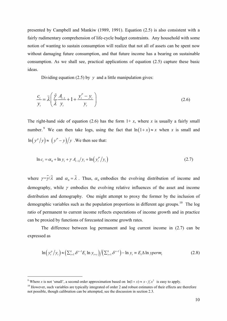
Dividing equation (2.5) by and a little manipulation gives: y

1 1P

t t t

t t t

c A yy y y

γλλ

−⎛ ⎞−

= + +⎜⎝ ⎠

ty⎟ (2.6)

The right-hand side of equation (2.6) has the form 1+ x, where x is usually a fairly small

number. 9 We can then take logs, using the fact that ( )ln 1 x x+ ≈ when x is small and

( )ln py y ≈ ( )Py y− y .We then see that:

(0 1ln ln ln Pt t t t tc y A y yα γ −= + + + )ty (2.7)

where = / γ γ λ and 0α λ= . Thus, 0α embodies the evolving distribution of income and

demography, while γ embodies the evolving relative influences of the asset and income

distribution and demography. One might attempt to proxy the former by the inclusion of

demographic variables such as the population proportions in different age groups.10 The log

ratio of permanent to current income reflects expectations of income growth and in practice

can be proxied by functions of forecasted income growth rates.

The difference between log permanent and log current income in (2.7) can be

expressed as

( ) ( ) ( )1 11 1ln ln ln lnp k s k s

t t s t t s s t ty y E y y E ypermδ δ− −= + =≈ ∑ ∑ − ≡ Δ t

(2.8)

9 Where x is not ‘small’, a second order approximation based on 21

2ln(1 ) - x x x+ ≈ is easy to apply. 10 However, such variables are typically integrated of order 2 and robust estimates of their effects are therefore not possible, though calibration can be attempted, see the discussion in section 2.3.

10

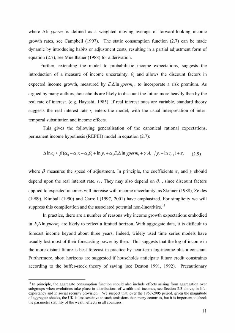
where is defined as a weighted moving average of forward-looking income

growth rates, see Campbell (1997). The static consumption function (2.7) can be made

dynamic by introducing habits or adjustment costs, resulting in a partial adjustment form of

equation (2.7), see Muellbauer (1988) for a derivation.

ln typermΔ

Further, extending the model to probabilistic income expectations, suggests the

introduction of a measure of income uncertainty, tθ and allows the discount factors in

expected income growth, measured by lnt tE ypermΔ , to incorporate a risk premium. As

argued by many authors, households are likely to discount the future more heavily than by the

real rate of interest. (e.g. Hayashi, 1985). If real interest rates are variable, standard theory

suggests the real interest rate enters the model, with the usual interpretation of inter-

temporal substitution and income effects.

tr

This gives the following generalisation of the canonical rational expectations,

permanent income hypothesis (REPIH) model in equation (2.7):

0 1 2 3 1 1ln ( ln ln ln )t t t t t t t t tc r y E yperm A y c tβ α α α θ α γ ε− −Δ ≈ − − + + Δ + − + (2.9)

where β measures the speed of adjustment. In principle, the coefficients 3α and γ should

depend upon the real interest rate, rt . They may also depend on tθ , since discount factors

applied to expected incomes will increase with income uncertainty, as Skinner (1988), Zeldes

(1989), Kimball (1990) and Carroll (1997, 2001) have emphasized. For simplicity we will

suppress this complication and the associated potential non-linearities.11

In practice, there are a number of reasons why income growth expectations embodied

in lnt tE ypermΔ are likely to reflect a limited horizon. With aggregate data, it is difficult to

forecast income beyond about three years. Indeed, widely used time series models have

usually lost most of their forecasting power by then. This suggests that the log of income in

the more distant future is best forecast in practice by near-term log-income plus a constant.

Furthermore, short horizons are suggested if households anticipate future credit constraints

according to the buffer-stock theory of saving (see Deaton 1991, 1992). Precautionary

11 In principle, the aggregate consumption function should also include effects arising from aggregation over subgroups when evolutions take place in distributions of wealth and incomes, see Section 2.3 above, in life-expectancy and in social security provision. We suspect that, over the 1967-2005 period, given the magnitude of aggregate shocks, the UK is less sensitive to such omissions than many countries, but it is important to check the parameter stability of the wealth effects in all countries.

11

behaviour with uncertain ‘worst case scenarios’ also generates buffer-stock saving, as in

Carroll (2001), who argues that plausible calibrations of micro-behaviour can give a practical

income forecasting horizon of about three years - as Friedman (1957, 1963) suggested.

The log formulation of the consumption function is very convenient with exponentially

trending macro data, since residuals are likely to be homoscedastic. Adding further realistic

features, splitting up assets into different types and introducing a role for the credit channel,

gives rise to a modern empirical version of the Friedman-Ando-Modigliani-Brumberg

consumption function that encompasses the basic life-cycle model given in (2.7):

( )

0 1 1 2 3

1 1 2 1 3 1

1 2 1

ln ln ln ln

ln

()

t t t t t t t t t t

t t t t t t t

t t t t t t t

c y c r E yNLA y IFA y HA y

y nr DB y

tpermβ α α α θ αγ γ γβ β ε

−

− − −

−

Δ ≈ + − + + + Δ

+ + +

+ Δ + Δ + (2.10)

Note that many of the parameters are time varying. The time variation induced by shifts in

credit availability is discussed below. 1tNLA y− t y is the ratio of liquid assets minus debt to

non-property income, 1t tIFA y− is the ratio of illiquid financial assets to non-property

income, and 1tHA y− t is the ratio of housing wealth to non-property income. ( )1t t tnr DB y−Δ ,

where is the nominal interest rate on debt , measures the cash flow impact on

borrowers of changes in nominal rates. The speed of adjustment is

tnr tDB

β and the γ parameters

measure the marginal propensity to consume (MPC) for each of the three types of assets. The

term in the log change of income can be rationalized by aggregating over credit constrained

and unconstrained households (see Muellbauer and Lattimore, 1995).12

The credit channel enters the consumption function through the different MPCs for

net liquid assets (Otsuka, 2006) and for housing; through the cash flow effect for borrowers;

and by allowing for possible parameter shifts stemming from credit market liberalization.

Credit market liberalization should (i) raise the intercept 0α , implying a higher level of

( )ln c y ; (ii) lower the real interest rate coefficient, thereby raising 1α ; (iii) raise 3α by

increasing the impact of expected income growth; and (iv) increase the MPC for housing

collateral, 3γ . It should also lower the current income growth effect, 1β and the cash flow

12 Note that 1 2 1 2 3 1 21, 0, , 0t t t t tβ α α γ γ γ β β= = = = = = = and 3 1tα = are the restrictions which result in the basic life-cycle/permanent income model equation (2.7).

12

impact of the change in the nominal rate, 2β . In our work on the UK, we handle these shifts

by writing each of these time-varying parameters as a linear function of the index of credit

supply conditions, CCI so that CCI enters the model both as an intercept shift and interacted

with several economic variables.

3. UK Results

3.1 Income-Forecasting Equations

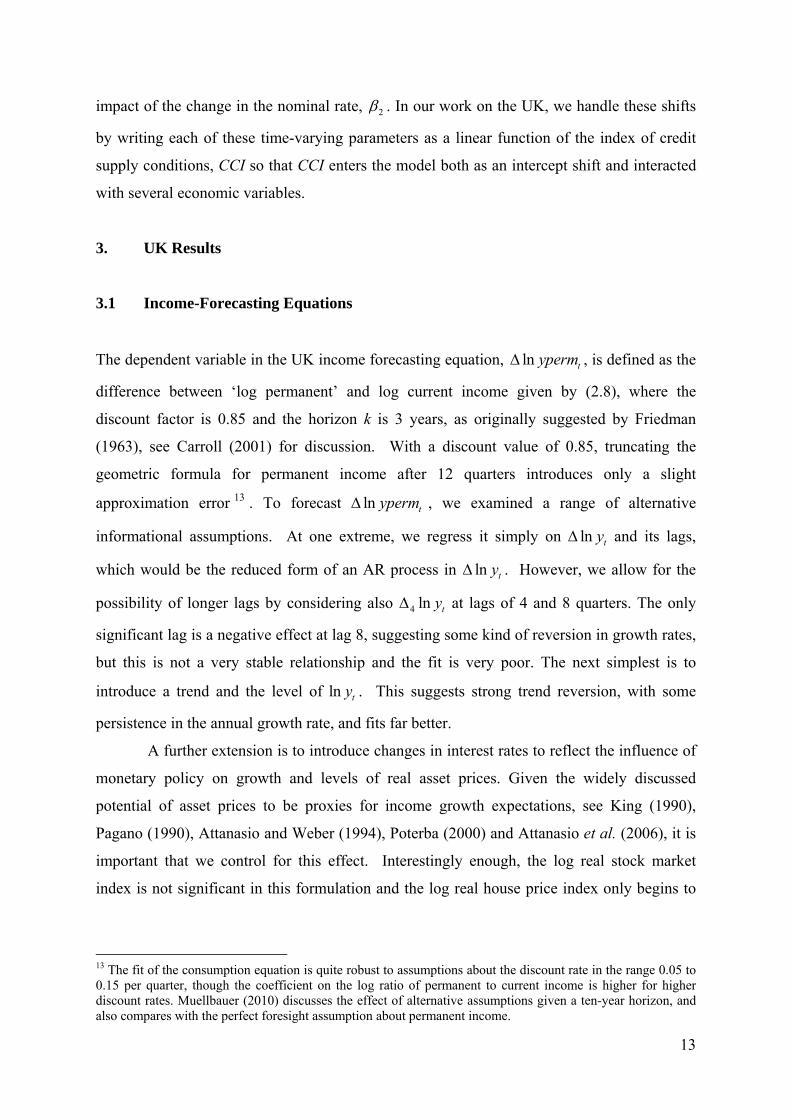
The dependent variable in the UK income forecasting equation, ln typermΔ , is defined as the

difference between ‘log permanent’ and log current income given by (2.8), where the

discount factor is 0.85 and the horizon k is 3 years, as originally suggested by Friedman

(1963), see Carroll (2001) for discussion. With a discount value of 0.85, truncating the

geometric formula for permanent income after 12 quarters introduces only a slight

approximation error 13 . To forecast ln typermΔ , we examined a range of alternative

informational assumptions. At one extreme, we regress it simply on and its lags,

which would be the reduced form of an AR process in

lnΔ ty

ln tyΔ . However, we allow for the

possibility of longer lags by considering also 4 ln tyΔ at lags of 4 and 8 quarters. The only

significant lag is a negative effect at lag 8, suggesting some kind of reversion in growth rates,

but this is not a very stable relationship and the fit is very poor. The next simplest is to

introduce a trend and the level of ln . This suggests strong trend reversion, with some

persistence in the annual growth rate, and fits far better.

ty

A further extension is to introduce changes in interest rates to reflect the influence of

monetary policy on growth and levels of real asset prices. Given the widely discussed

potential of asset prices to be proxies for income growth expectations, see King (1990),

Pagano (1990), Attanasio and Weber (1994), Poterba (2000) and Attanasio et al. (2006), it is

important that we control for this effect. Interestingly enough, the log real stock market

index is not significant in this formulation and the log real house price index only begins to

13 The fit of the consumption equation is quite robust to assumptions about the discount rate in the range 0.05 to 0.15 per quarter, though the coefficient on the log ratio of permanent to current income is higher for higher discount rates. Muellbauer (2010) discusses the effect of alternative assumptions given a ten-year horizon, and also compares with the perfect foresight assumption about permanent income.

13

be relevant from 1981, after the advent of UK credit market liberalisation. The estimated

equation with these elements is used to generate a ‘naïve’ forecast.

At the other extreme, we posit a long-run relationship for ln as a function of a

linear trend (+), real interest rates (-), changes in nominal interest rates (-), the logs of real oil

prices (-), share prices (+) and real house prices (+), the rate of tax on income (-), the rate of

unionization (+) since greater union power should raise the share of labour income, and some

national accounts ratios. These include the ratio of the government surplus to GDP where a

higher ratio in the long run should allow lower tax rates or higher government spending,

though offset in the short run by the negative ‘Keynesian’ effect of fiscal contraction, and the

ratio of the trade deficit to GDP, since trade deficits have in the past constrained growth.

However, there was a profound shift in fiscal policy around 1980, with the coming into

power of the Thatcher government. This would be expected to have reinforced the positive

role of the government surplus, and with the Burns-Lawson doctrine

ty

14, to have led to trade

deficits no longer mattering for fiscal policy. We find strong evidence for both hypotheses by

testing for interaction effects with pre and post 1980 dummies. We also test for a shift in the

early 1980s in the role of real house prices, to be consistent with the shifting role of housing

wealth in consumption with credit market liberalization. We confirm the absence of a positive

real house price effect on income before the early 1980s, as in the ‘naïve’ model. We also

checked for world growth and real exchange rate effects but failed to find stable relationships.

The long run level effects discussed all enter as four-quarter moving averages, though

for oil prices, the lags are even longer. Using a general-to-specific reduction procedure with

HAC t-ratios and F-tests, we check for short run dynamics from changes in interest rates,

where negative effects are confirmed, and growth rates of income and real oil and asset prices,

in part to check for dynamic mis-specification due to the choice of four-quarter moving

average level effects. We take the simple average of the forecasts from this sophisticated

model and the ‘naïve’ model discussed above to measure the predicted value of permanent to

current income.

3.2 The Estimated UK Consumption Equation

14 The doctrine states that with free global capital flows, governments should concern themselves with budget deficits, but not with trade deficits and let these be a matter for the private sector. Terence Burns as chief economic advisor and Nigel Lawson as chancellor, made the doctrine official policy. Exchange controls were removed in 1979.

14

We begin by estimating our version of the text-book rational expectations permanent income

model given by equation (2.10), with quarterly data. Consumption refers to real per capita

consumer spending, including durables. Income is real per capita non-property income 15.

The net worth to income ratio is defined as liquid assets minus debt plus illiquid financial

assets plus housing wealth, taken as the end of previous quarter levels, relative to current

income.

--- Table 1 About Here ---

In Table 1, column 1 shows the text-book REPIH model with habits, equation (2.9)

but omitting income uncertainty and the real interest rate, with highly significant estimates of

net worth and income growth expectations effects and a speed of adjustment of 0.16 per

quarter.16 The long-run marginal propensity to consume out of net worth is obtained by

dividing its coefficient 0.0036 by the speed of adjustment 0.16, to give 0.022. Column 2

shows one relaxation of the text book model, in which the ratio to income of net liquid assets,

defined as liquid assets minus debt, is permitted to have a different coefficient from illiquid

assets. This radically affects the size of the wealth effects, with the marginal propensity to

consume out of net liquid assets equalling 0.11 and that out of illiquid assets estimated at

0.033, rather than the 0.022 implied by column 1. The speed of adjustment rises to 0.23 and

the improvement in fit clearly rejects the text-book model in column 1. In column 3, we

report on estimates of equation (2.10) again without including CCI or its interaction with any

other variables. The additional variables are the change in the unemployment rate, a proxy

for income insecurity, the real interest rate, the weighted change in nominal interest rates on

debt, and a separate housing ‘wealth’ effect. Though the real interest rate is insignificant, the

other effects are all significant and the marginal propensity to consume out of housing wealth

effect is apparently larger at 0.036 than out of illiquid financial assets at 0.023. Clearly, the

superior fit of this model rejects the restrictions embodied in columns 1 and 2.

Finally, we show a specification in column 4 in which we allow the relevant

parameters of equation (2.10) to shift with the UK index of credit conditions, CCI. The

expected shifts in parameters all occur, though some are insignificant. Overall, the

15 Defined as personal disposable income minus approximately tax-adjusted property income. 16 All specifications reported in Table 1 also include an intercept, dummies for temporary shifts in consumption due to sales tax anticipations, a measure of the change in consumer credit controls for durables purchases, and a measure of working days lost in labour disputes. A data appendix with sources, summary statistics and unit root tests for all three countries is available upon request.

15

improvement in fit is significant relative to column 3. We show a parsimonious version of

the model. The housing wealth-to-income ratio is insignificant, while its interaction effect17

with CCI is strongly significant, and so we omit the former. The marginal propensity to spend

out of housing assets at the maximum value of CCI (normalized at 1) is 0.032, while that of

illiquid financial assets is around 0.019, which, in turn, is far below that of net liquid assets,

at around 0.11. These results for the housing assets effect are lower than many found in the

literature. We find that a four-quarter moving average of observations on illiquid financial

assets fits a little better than the end of previous quarter value, consistent with findings by

Lettau and Ludvigson (2004).18 Since much of illiquid financial assets lies in pension funds,

this plausibly reflects the slow adaptation of contribution and pay-out rates to changes in

asset values.

The real interest rate effect is negative, but significant only at the 10 percent level.

According to point estimates, not shown, the evidence is that it strengthens as CCI rises. The

debt-weighted nominal interest rate change, also negative, weakens as CCI rises. With easier

access to credit, inter-temporal substitution should play a bigger role, explaining, as noted

above, the enhanced role for income growth expectations, for which there is also evidence

here. Income uncertainty is represented by the four quarter change in the unemployment rate,

which has a negative effect on consumption. The interaction effect with CCI is positive, but

quite insignificant, suggesting that higher debt levels have offset the reduction in income

uncertainty effects one might have expected from easier access to credit. The speed of

adjustment is 0.33 meaning that 80 percent of the adjustment of consumption to income and

the other explanatory variables is complete after four quarters.

The parameters of this equation are remarkably stable as charts of recursive estimates

reveal.19 The model can be interpreted in terms of co-integrated variables. Effectively, the

log ratio of consumption to non-property income and the three asset to income ratios form a

co-integrated relationship between four I(1) variables, subject to a shift in the intercept via

CCI. Since the real interest rate is arguably I(0) and in any case plays only a marginal role,

we can neglect it here. We carried out a co-integration analysis, in which we treat CCI as an

exogenous shift dummy, and include in the equation system I(0) variables such as income

17 This interaction effect takes the form (housing wealth/income minus the mean value of this ratio from 1980 to 2005) multiplied by CCI. The post-1980 mean value of the housing wealth-to-income ratio is 3.08, compared to a 2005Q4 value of 4.71. 18 However, over a one or two year horizon, the estimated stock market effect on consumption of Lettau and Ludvigson is implausibly small. 19 Charts are available on request.

16

growth and forecast growth and the change in the unemployment rate and the impulse

dummies, but outside the co-integration space. With a lag of two, there is only one co-

integrating relationship and this is close to the long-run solution implied by the column 4

estimates. Effectively, this analysis treats current income growth and the forecast of future

growth and the unemployment rate as weakly exogenous variables. Evidence for weak

exogeneity is found from models for these I(0) variables in which the lagged equilibrium

correction term implied by the co-integration vector is insignificant20. For the UK, therefore,

the pessimism expressed by Lettau and Ludvigson (2004) and Carroll et al. (2006) for the

existence of a cointegrating relationship between consumption, income and assets appears to

be misplaced, at least once the CCI effect is included and assets are split into the three

components indicated.

A further specification check on the model is to estimate it introducing a smooth

stochastic trend, to capture omitted demographic and other trending effects, see discussion

below for the US. Using the STAMP software (Koopman, Harvey, Doornik and Shephard,

2006), we find no indication of such a trend. This suggests that the net influence of such

omitted effects on consumption is small for the UK in this period, relative to the large

variations in asset prices, credit conditions, unemployment changes and other shocks. The

indications are that higher income inequality may have lowered the consumption to income

ratio while a higher proportion of adults aged over 65 may have raised it. But these trending

effects are hard to identify.

--- Figures 2 and 3 About Here ---

Figures 2 and 3 show the long-run contribution to the log consumption-to-income

ratio of the three asset to income ratios and of the credit conditions index, weighting each by

its estimated long-run coefficient. As discussed further below, it should be noted that these

are not general equilibrium effects. Figure 2 suggests that a substantial part of the upturn in

consumption relative to income can be attributed to the rise in the credit conditions index and

that some of the upturn in consumption relative to income from 1984 to 1989 and much of

the upturn from 1995 to 2005 can be attributed to the rises in the collateral values of homes

relative to income. The role of income growth expectations was far smaller. Indeed, as

20 While income is likely to be endogenous for consumption, on the UK data, current quarter growth of real income appears to be weakly exogenous for the log consumption to income ratio.

17

Muellbauer (2010) shows, they had a negative effect on the consumption to income ratio in

1984-89, though their role was positive in 1995-2005.

Figure 3 further suggests that the upward trend in the value of illiquid wealth holdings

relative to income also played in important part in the upward trend in consumption relative

to income. However, the rise in debt, reflected in the fall of net liquid assets relative to

income seen in Figure 3, has major offsetting effects in the long run21. The fact that the

estimated marginal propensity to consume out of net liquid assets is substantially higher than

that out of other assets is quite important here. Much conventional discussion of wealth

effects focuses on net worth and so misses the special role of liquidity and of debt. Figure 3

suggests that, as discussed in the Introduction, UK consumption levels are now quite

vulnerable to downturns in asset prices, given that debt is hard to reduce in the short- run22.

4. Results for Japan

4.1 The income growth forecasting equations.

For Japan, we work with annual data. In practice, it made little difference whether we use the

one-year-ahead growth rate of income, or a weighted average of up to three years ahead, to

model . We follow a general to specific methodology in paring down a very general

model to a parsimonious form. The general model includes a trend, a split trend from 1973

for the slowdown in Japanese growth which then occurred and the level of log real per capita

income. Other variables checked included log US GDP, the log real exchange rate, log real

oil prices, log real asset prices, the real interest rate, the change in the nominal interest rate,

and the government surplus and debt to GDP ratios

ln( / )Pt ty y

23.

There is strong evidence for reversion to the split growth trend and the 3-year moving

average of government balance/GDP has a positive coefficient. The log of US GDP is also

significant and real oil prices are then not significant, though they would be if US log GDP

were omitted. The influence of the US as leading economy and key trading partner for Japan

is thus confirmed. The change in nominal interest rates over the previous three years has a

21 As Ed Lazear and William White commented on Muellbauer (2007) at the 2007 Jackson Hole Symposium, if the house price effect on consumption is mainly a collateral effect, payback time has to come. This is reflected in Figure 3. 22 Note that at mid-2007 illiquid financial assets relative to income were substantially above the 2005 ratio shown in Figure 3, but have fallen sharply since. 23 Results are available from the authors upon request.

18

negative effect on next year’s household income growth, suggesting that, overall, monetary

policy has some negative effect on growth. However, the real interest rate is insignificant,

and positively signed. The ratios to GDP of the government surplus or of the level and

change in government debt to income are highly significant, consistent with a partially

Ricardian view of households. The income forecasting equations fitted over alternative

samples, show remarkable parameter stability.

4.2 Results for Aggregate Japanese Consumption

Our aim is to estimate for Japan variants of equation (2.10) discussed in section 2. We use

annual data from 1961 to 2006. In a slight modification, we also include the lagged log real

land price. It quickly becomes apparent that the real land price has a negative coefficient.

On the other hand, the physical asset to income ratio is not significant and is thus omitted.

Further, we cannot reject the hypothesis that the marginal propensities to spend out of

deposits and illiquid financial assets are the same, and are equal to minus the coefficient on

household debt. This may be because “deposits” includes a substantial amount of longer

term time deposits which are therefore not so liquid. Thus, we can work with net financial

wealth, which is always very significant and with a long run MPC of around 0.05 to 0.07 (see

Table 2).

--- Table 2 About Here ---

The income uncertainty indicators (the unemployment rate and income volatility)

enter with the correct signs.24 The measure of income volatility is significant as shown in the

first column of Table 2. In the second column the cross term of income volatility and

forecast income growth rate was added, as the theory discussed in Section 2 suggests that

greater income uncertainty should lead to a bigger discount on expected growth. When both

are included, the cross term was found to be significant while income volatility insignificant.

The change in the unemployment rate is not significant at the 5% level, probably because of

its more limited variability in Japan, in contrast to its far more significant role in the UK and

the US. However, the sign is negative and the magnitude of the coefficient is not far below

UK and US estimates. 24 Income volatility is defined as the absolute value of discrepancy between the current income growth and its moving average over the previous five years (including current year).

19

The change in the nominal interest rate is always insignificant, unlike in the UK, but

the level of the real rate has a strongly significant positive effect. This is not a disguised

inflation effect as the inflation rate is insignificant when included, while the real rate remains

significant. Finally, the log change in income has a positive and significant effect. This is

also in contrast to the UK and US findings, where this effect is not significant. The argument

comes from applying the Campbell-Mankiw aggregation of credit constrained and

unconstrained households to a solved out consumption function, see Muellbauer and

Lattimore (1995). On this interpretation, the proportion of total income in income constrained

households π is given by ( ) 11 π β β− = , where the coefficient on the change in log income is

1β and β is the speed of adjustment. Given a speed of adjustment of 0.359 and 1β estimated

at 0.332 from Table 2 column 4, this suggests just over half of Japanese consumption comes

from households who are, or behave as if they were, income constrained. This is not far

from previous estimates of this proportion for Japan, see Hayashi (1997). However, given

the somewhat unsatisfactory micro foundations for the Campbell-Mankiw story, it is

probably a mistake to interpret this too literally in terms of credit constraints (see Carroll,

2001).

In Muellbauer and Murata (2010), various charts of the fit of the equation over the full

sample and recursive parameter estimates are presented. The stability properties of the

equation are excellent when the equation is estimated over different samples. Together, these

provide clear support for the long-term relevance of the model, though in short samples the

real land price effect loses significance, given its lack of short-term variability.

This raises the question of whether there may have been a structural break in the

coefficient on log real land price. We test for this by interacting the lagged log real land price

with two step dummies, the first equal to zero up to 1980, and to one thereafter; the second

equal to zero up to 1990, and to one from 199125. The results hardly alter when the latter

step dummy was replaced by the former. The coefficient on the step dummy interaction

effect is not significant, with a t-ratio of 0.7. The point estimate is consistent with a small

amelioration in the negative impact of land prices on consumption after 1991 (and indeed

after 1981). But we can easily accept the hypothesis of constancy of the negative real land

price effect.

25 To avoid a jump in the interaction effect in, for example, 1991, the 1991 step dummy is multiplied by the lagged log land price index minus its 1990 value.

20

--- Figures 4 and 5 About Here ---

Lower income growth and the uncertainty indicators explain some of the dramatic

decline in the consumption to income ratio in the 1970s. The long-run contributions of the

four I(1) explanatory variables – the net financial wealth to income ratio, the log real land

price, the real interest rate and the forecast growth rate of income, are shown in Figures 4 and

5. It is clear from this figure that the rise of the consumption to income ratio is very much

driven by the rise in net financial assets owned by households, only somewhat offset by the

rise in real land prices. Interestingly, net financial assets relative to income shows rather

little cyclical variation, as the pension fund component is not very sensitive to the stock

market, though its decline in the early 1990s also contributed to the drop in the consumption

ratio then.

It is a striking fact that demographic variables, such as the share of the population

aged 25 to 44 or 65 and over, are jointly and individually insignificant when included in the

consumption equation.26 This does not mean, of course, that demographic developments are

irrelevant for aggregate consumption in Japan. The accumulation of financial wealth in Japan

in the past has surely been, in part, driven by the ageing of the population and lengthening

life-expectancy. Consumption or saving, conditional on such portfolio accumulations, is

always less likely to be so sensitive to demographic structure.

5. US Results

5.1 Income Forecasting Equations

As for the UK, we estimate equations for the deviation of log ‘permanent’ income from

current log income, see equation (2.8). Income is real per capita non-property income as

constructed for the FRB-US model.27 For expectations of the deviation of permanent income

from current income, we use a simple model based on reversion to a split trend (with a slow-

down in growth from 1968) with just two economic drivers. These are the four-quarter

26 Moreover the signs often make little sense. What does make more sense is the inclusion of the proportion of the adult population aged 25 to 44. These are the main savers for a housing deposit. A rise in their proportion tends to lower consumption relative to income, though the effect still only has a t statistic of -1.1. Micro evidence, see Hayashi (1997), indicates that older Japanese households tend to carry on saving until their 80s, but perhaps the 25 to 44 group are the biggest savers. 27 Non-property income is defined as tax-adjusted labour income plus transfer income. The particular variant used is adjusted, following Blinder and Deaton (1985), for temporary tax changes.

21

change in the 3 month Treasury bill yield, representing the impact of monetary policy, and a

Michigan survey measure of consumer expectations28. This has the advantage of being based

on a survey of actual consumers. Permanent income was constructed with three alternative

quarterly discount rates, 0.025, 0.05 and 0.1. There is little difference in fit between the last

two and so a discount rate of 0.05 was chosen. It suggests consumers have short horizons,

which is consistent with a high degree of uncertainty about the future. Figure 6 shows actual

and fitted or forecast values.

5.2 Consumer Credit Index for the US.

The first issue we address is the measurement of shifts in the credit supply function facing

households. The closest US source for micro data on mortgage loan-to-value (LTV, or its

equivalent, down-payment to value) and on loan-to-income ratios (LTI), used by Fernandez-

Corugedo and Muellbauer in the UK context, is the American Housing Survey. However, the

sample is far smaller than the UK survey of mortgage lenders and LTV data are usable only

from 1979, too short a period to analyse consumption from 1972. Nevertheless, as neither

LTV nor LTI ratios rose much from 1979 to 1998 it does suggest that, for first time buyers in

the US before 1998, the easing of mortgage credit conditions may have been less dramatic

than for the UK, see Duca et al. (2010a).

One data advantage the US has over the UK is the Federal Reserve’s quarterly Senior

Loan Officer Opinion Survey. For the US, a credit conditions index (CCI) is constructed from

a quarterly diffusion index (CR) tracking the net relative change in bank willingness to make

consumer instalment loans over the prior three months across 60 large banks in this survey.

This index is negatively and significantly correlated with a diffusion index from the same

survey of the net percentage of banks that tightened credit standards on non-credit card

consumer loans, available since 1993. Before constructing a levels index from this relative

change index, we first adjust it for identifiable effects of interest rates and the

28 The Index of Consumer Expectations (ICE) is calculated by first computing the relative scores (the percent giving favourable replies minus the percent giving unfavourable replies, plus 100) for questions two through four as follows: (2.) Now looking ahead--do you think that a year from now you (and your family living there) will be better off financially or worse off, or just about the same as now? (3.) Now turning to business conditions in the country as a whole--do you think that during the next 12 months we'll have good times financially, or bad times, or what? (4.) Looking ahead, which would you say is more likely--that in the country as a whole we'll have continuous good times during the next five years or so, or that we will have periods of widespread unemployment or depression, or what? Each relative score is then rounded to the nearest whole number. The sum of the three relative scores is divided by the 1966 base period total of 4.1134 and then 2.0 (a constant to correct for sample design changes from the 1950s) is added to the result.

22

macroeconomic outlook by estimating an empirical model based on screening models (see

Appendix). This adjusted index of the relative change in the availability of consumer

instalment loans is aggregated into a levels index based on 1966-82 correlations of the index

with the growth rate of real consumer loan extensions at banks. The resulting CCI rises

greatly during the 1980s, and then rises during the height of the subprime mortgage boom

2004-06, before reversing the gains of the early decade since 2006 (see Figure 7). While the

index is tailored to consumer instalment credit rather than mortgage markets, it can serve as a

first approximation to a more general credit conditions index.

5.3 Consumption Function Estimates for the US.

A sequence of models was estimated for the US of a similar form to the UK consumption

functions. The results are shown in Table 3.29 The simplest specification is based on a simple

extension of the traditional life-cycle model with habits (Table 3, column 1). The dependent

variable is the log change in real per capita consumption excluding consumption of housing

services. The regressors include ln y-ln c-1, the log change in real per capita non-property

income (to reflect the possibility that some households simply spend income), our proxy for

permanent income relative to current income, a dummy for oil shocks from Mideast

disturbances30 and the ratio of net worth (at the end of previous quarter) to income. A

dummy was also added for the outlier in 1980q2 for the imposition of credit controls. The

estimated long-run MPC for net worth is 0.04, a number in line with conventional wisdom.

The speed of adjustment is very low, however, at 0.096 per quarter, and the role of current

income growth is dominant. The residuals suffer from serious autocorrelation. Column 2

breaks up wealth into its three components with little change in key coefficients. Column 3

adds the change in the unemployment rate, the change in the nominal interest rate and the

level of a real interest rate, as in the UK. The interest rate is the auto-finance rate, which

reflects special offers sometimes available to borrowers. The changes in the unemployment

rate and in the nominal interest rate are highly significant, as in the UK, and reduce some of

the specification problems seen in columns 1 and 2. Much of the interest rate effect may

reflect short-term inter-temporal substitution induced by special auto sales finance programs.

29 Very similar qualitative results for U.S. consumption in Table 3 were obtained in corresponding models, shown in Appendix Table 1, which replace current income and income expectations with their t-1 lags. This suggests that the endogeneity of current income is not an issue. 30 The dummy OILSHOCK equals 1 in 1973:q4, 1974:q1, 1979:q2, 1979:q3, and 1990:q4); and 0, otherwise.

23

--- Table 3 About Here ---

In column 4, the credit conditions index is added. The credit conditions index is

significant and the speed of adjustment more than doubles to 0.196, suggesting a better

specified long-run solution. The role of current income growth is now far lower, comparing

columns 1 through 4. Concerning the wealth effects, the data suggest that all components of

wealth are significant, and have a similar MPC. This seems implausible since cash (liquid

assets) should be more spendable than illiquid financial assets and housing assets, which,

even if used as loan collateral rather than sold outright, entail the transactions costs of

arranging loans.

One explanation is that there are time-varying degrees with which US households can

use housing wealth as collateral, and ignoring this aspect biases the wealth effects. Ideally,

the equation would include a credit conditions index specific to the mortgage market. The

estimated effect of liquid wealth in column 4 is likely to be biased down by the omission of

such a mortgage credit conditions index. Since the early 1980s, the ratio of net liquid assets

to income has fallen almost monotonically, induced in part by easier mortgage credit

conditions. The latter has a positive effect on consumption, but is negatively correlated with

the ratio of net liquid assets to income, supporting the argument of a downward bias on the

coefficient on net liquid assets.

A simple check on the column 4 specification is to add a smooth stochastic trend,

estimated with the STAMP software (Koopman, Harvey, Doornik and Shephard, 2006). This

proves to be significant, evidence of a missing trending factor. The costs of refinancing fixed

interest rate US mortgages fell in the 1990s, as shown by Bennett, Peach, and Peristiani

(2001) and Green and Wachter (2007), who review changes in US mortgage markets from a

longer perspective. Duca et al. (2010b) estimate the latent costs of refinancing US mortgages

since the 1970s. They find these costs shifted down substantially in the late 1990s, making it

more feasible to refinance mortgages and increasing the collateral value of housing wealth.

Thus, credit market liberalisation may have altered the spending power of housing wealth or

collateral. Column 5 explores the role of housing collateral by interacting housing wealth

with the housing liquidity index (HLI, see Figure 8) of Duca et al. (2010b). The fit and speed

of adjustment of this model are notably better than in column 4.

There are some notable differences in the model properties that are more consistent

with theory. First, the effect of liquid assets is larger, with an MPC of 0.133, far higher than

that of illiquid financial wealth, and broadly consistent with microeconomic evidence from

24

Gross and Souleles (2002). Second, non-interacted housing wealth has a negative effect on

non-housing consumption, but it is significant and positive when interacted with HLI,

consistent with housing wealth having a collateral channel effect on non-housing

consumption. This finding is consistent with both theory (Muellbauer and Lattimore, 1995)

and the micro evidence finding that observed housing wealth effects result from greater

housing collateral (Browning et al., 2009).

The results in Table 3 suggest that the marginal propensity to consume out of housing

wealth in recent years substantially exceeds that out of illiquid financial wealth. This

supports the finding of Case et al. (2005) for the US that the housing wealth (or collateral)

effect exceeds the stock market wealth effect, and the results are consistent with Benjamin et

al. (2004) and Carroll et al. (2006).

It is noteworthy that the UK and US figures are roughly similar. In the UK, the MPC

for net liquid assets is estimated at 0.11, and the US estimate of 0.133 (Table 3, column 5) is

close. The MPC for housing collateral in the UK is close to 0.032. Our most plausible US

estimate peaks near 0.036.31 Most values estimated for the US, are substantially higher.

The similar estimates of the marginal propensity to consume out of housing wealth

suggest that the influence of any differing structural aspects across UK and US housing and

mortgage markets roughly cancel out in the aggregate. On the one hand, transactions fees of

US real estate agents (about 6 percent) are larger than the transactions tax rates (Stamp Duty)

in the UK, implying greater housing liquidity in the UK. On the other hand, in case of

default, mortgage borrowers are more liable for compensating lenders for mortgage losses in

the UK than on average in the US. In many states (such as California), lenders have recourse

only to the house collateralizing the mortgage, which may make housing more attractive to

borrow against.

An important paper by Slacalek (2009) presents estimates of housing ‘wealth’ or

collateral effects on consumption for a range of countries, using a different methodology. His

evidence suggests that institutional differences between countries have large effects on the

MPC out of housing wealth, far larger in countries with liberal mortgage markets. This

concurs with our evidence for Japan, the UK and the US. His evidence, like ours, is also

consistent with an upward drift over time in the MPC, linked with credit market liberalisation.

His estimates of the MPCs for housing wealth for US or UK-style economies are far larger

than ours, perhaps from omission of a credit conditions index, creating an upward bias.

31 The non-interactive housing wealth coefficient of -.0050 plus the peak value (1.0) of the housing liquidity index multiplied by the coefficient on interactive housing wealth and divided by the speed of adjustment.

25

26

6. Concluding comments

Consistent with theory, our empirical findings for the UK, US, and Japan demonstrate the

importance of credit constraints for consumer spending. We find that the evolution of credit

availability differs over time within countries, as well as between them. In Japan, the

consumption function has been stable, reflecting a lack of household credit liberalization

since the 1970s. The latter and differences in the tax code likely account for the restraint on

consumption in Japan from rising home prices.

In contrast, there have been large changes in the availability of credit to UK and US

households over the last few decades. Improved access to credit has shifted up the

consumption function in both countries. Furthermore, financial liberalization has enhanced

the positive impact of housing wealth on consumption in the UK and US. and the role of

expected income growth in the UK.

Comparing Japan with the UK and the US, the consumption function differences

suggest that monetary policy transmission via the household sector is far less powerful and

perhaps even perverse in Japan. Large household liquid asset holdings in Japan relative to

debt imply that households, older households in particular, feel poorer when short term

interest rates fall and so reduce spending. In the US and UK, where debt exceeds liquid assets,

higher spending by debtors more than offsets this effect. To the extent that lower interest

rates raise house prices, this also has a (small) negative effect on aggregate household

spending as Japanese renters save more in anticipation of higher future rents or of higher

down-payments to obtain a mortgage. In the US and UK, in contrast, greater possibilities for

housing equity withdrawal with higher collateral values boost spending. The conventional

positive effects of lower short term interest rates on household spending via financial asset

prices and income growth expectations apply in Japan as in the UK and US.

Our findings suggest that the impact of the large, recent declines in wealth,

particularly in housing equity, will have strong and persistent dampening effects on consumer

spending in the UK and the US. Volatile housing wealth also reflects the impact of changes

in mortgage credit standards. During the recent recession, negative wealth effects were

compounded by a substantial tightening of consumer credit standards in the US, a

combination not seen since 1974-75, when consumption was unusually weak (see Duca et al.,

2010a). In both episodes, mortgage availability declined sharply. In the UK, a tightening of

credit standards has resulted in sharp rises in loan-to-value and loan-to-income ratios for first-

time home-buyers, contributing to sizeable declines in house and other asset prices from

27

historic highs. More recently, cuts in interest rates to historic lows have provided an

important counterweight.

Japanese consumer spending is less likely to be directly affected, if at all, by falling

Japanese housing wealth and credit availability. Nevertheless, the global economic downturn,

particularly in the US, proved detrimental to Japanese household income due to declines in

net exports. Moreover, the damage from loan losses at financial institutions have been large

enough to induce credit tightening and lower financial asset prices outside of the US

(Greenlaw, Hatzius, Kashyap, and Shin, 2008).

Striking similarities between the consumption functions for the UK and the US and

their contrast with Japan emphasises the importance of institutional differences. This

underlines the contribution of the generalised version of the Ando-Modigliani-Brumberg

consumption function, which unlike the textbook Euler equation approach, incorporates

credit frictions, uncertainty and income expectations. Household balance sheet data,

neglected in many macroeconomic models, are critical. Without carefully accounting for

evolving credit and wealth relationships, the impact of credit and financial shocks on

household spending and the monetary transmission mechanism cannot be properly modelled

or understood.

References

Ando, A. and Modigliani, F. (1963), "The ‘Life Cycle’ Hypothesis of Savings: Aggregate

Implications and Tests," American Economic Review, 53, 55-84. Aron, J. and Muellbauer, J. (2000), "Personal and Corporate Saving in South Africa,” World Bank

Economic Review, 14(3), 509-44. Attanasio, O., Blow, L., Hamilton, R. and Leicester, A. (2009), “Booms and Busts: Consumption,

House Prices and Expectations,” Economica 76(301): 20-50. Attanasio, O. and Weber, G. (1994), “The UK Consumption Boom of the Late 1980s: Aggregate

Implications of Microeconomic Evidence”, Economic Journal, 104(1), 269–302. Benjamin, J., Chilloy, P. and Jud, D. (2004), “Real Estate Versus Financial Wealth in Consumption”,

Journal of Real Estate Finance and Economics, 29(3), 341-84. Bennett, P., Peach, R., and Peristiani, S. (2001), “Structural change in the mortgage market and the

propensity to refinance,” Journal of Money, Credit, and Banking 33(4), 955-75. Blinder, A. and Deaton, A. (1985), "The Time Series Consumption Function Revisited," Brookings

Papers on Economic Activity, 1985(2), 465-511. Bosworth, B., Burtless, G. and Sabelhaus, J. (1991), “The Decline in Saving: Evidence from

Household Surveys”, Brookings Papers on Economic Activity, 1991(1), 182-256. Brayton, F., Levin, A., Tryon, R. and Williams, J. (1997), “The Evolution of Macro Models at the

Federal Reserve Board”, Carnegie Rochester Conference Series on Public Policy, 47, 43-81. Browning, M., Gortz, M., and Leth-Petersen, S. (2009), “House Prices and Consumption: A Micro Study,” unpublished manuscript, Nuffield College, Oxford University. Buiter, W. (2008), “Housing Wealth Isn’t Wealth,” NBER Working Paper No. 14204, July.

28

Cameron, G., Muellbauer, J. and Murphy, A. (2006), “Was There a British House Price Bubble? Evidence from a Regional Panel”, Centre for Economic Policy Research (CEPR) discussion paper no. 5619.

Campbell, J. and Mankiw, N. (1989), “Consumption, Income and Interest Rates; Reinterpreting the Time Series Evidence”, in Blanchard, O. and Fischer, S. (eds.), NBER Macroeconomics Annual 1989, Cambridge, Mass: MIT Press.

Campbell, J. and Mankiw, G. (1991), “The Response of Consumption to Income: A Cross-Country Investigation,” European Economic Review, 35(4), 723-56.

Carroll, C. (1997), “Buffer Stock Saving and the Life Cycle/Permanent Income Hypothesis", Quarterly Journal of Economics, CXII(1), 1-56.

Carroll, C. (2001) "A Theory of the Consumption Function, with and without Liquidity Constraints," Journal of Economic Perspectives, American Economic Association, vol. 15(3), pages 23-45, Summer.

Carroll, C., Otsuka, M. and Slacalek, J. (2006), “How Large Is the Housing Wealth Effect? A New Approach", mimeo.

Case, K., Quigley, J. and Shiller, R. (2005), “Comparing Wealth Effects: The Stock Market Versus the Housing Market” Advances in Macroeconomics, 5(1), Article 1. Online at http://www.bepress.com/bejm/advances/vol5/iss1/art1.

Deaton, A. (1991), “Savings and Liquidity Constraints”, Econometrica, 59(5), 1221-48. Deaton, A. (1992), Understanding Consumption, Oxford: Clarendon Press. Deaton, A. (1999), “Saving and Growth”, in Schmidt-Hebbel, K. and Serven, L. (eds.), The

Economics of Saving and Growth, Cambridge: Cambridge University Press. Deaton, A. and Muellbauer, J. (1980), Economics and Consumer Behaviour, Cambridge University

Press. Duca, J., (2000), “Financial Technology Shocks and the Case of the Missing M2,” Journal of Money,

Credit, and Banking 32(4), 820-39. Duca, J. and Garrett, B (1995), “Credit Availability, Bank Consumer Lending, and Consumer

Durables,” Federal Reserve Bank of Dallas Working Paper No. 9514. Duca, J., Muellbauer, J. and Murphy, A. (2010a), “Home Prices and Credit Constraints: Making

Sense of the US Experience”, mimeo. Duca, J., Muellbauer, J. and Murphy, A. (2010b), “The Impact of the Financial Crisis on US

Consumption and Saving”, mimeo. Duca, J. V. and Wu, T. (2009), “Regulation and the Neo-Wicksellian Approach to Monetary Policy,”

Journal of Money, Credit, and Banking. 41(3), 799-807. Dynan, Karen E., Elmendorf, Douglas W., and Sichel, Daniel E. (2006), “Can Financial Innovation

Help to Explain the Reduced Volatility of Economic Activity?” Journal of Monetary Economics 53, 123-150.

Eichner, Matthew J., Kohn, Donald L., and Palumbo, Michael G. “Financial Statistics for the United States and the Crisis: What Did They Get Right, What Did They Miss, and How Should They Change?” Finance and Economics Discussion Series, working paper no. 2010-20.

Engelhardt, G. V. (1996), “Consumption, Down Payments and Liquidity Constraints,” Journal of Money Credit and Banking, 28(2), 255-71.

Fernandez-Corugedo, E. and Muellbauer, J. (2006), “Consumer Credit Conditions in the U.K.” Bank of England working paper 314.

Friedman, M. (1957), A Theory of the Consumption Function. Princeton: Princeton University Press. Friedman, M. (1963), “Windfalls, the ‘Horizon’ and Related Concepts in the Permanent Income

Hypothesis”, in Christ, C., Friedman, M., Goodman, L., Griliches, Z., Harberger, A., Liviatan, N., Mincer, J., Mundlak, Y., Nerlove, M., Patinkin, D., Telser, G. and Theil, H., (eds.) Measurement in Economics: Studies in Mathematical Economics and Econometrics in Memory of Yehuda Grunfeld, Stanford University Press.

Gokhale, J., Kotlikoff, L. and Sabelhaus, J. (1996), “Understanding the Postwar Decline in U.S. Savings: A Cohort Analysis”, The Brookings Papers on Economic Activity, 315-344.

Goldberger, A. S. (1974), “Unobservable Variables in Econometrics”, in Zarembka, P. (ed.), Frontiers of Econometrics, Academic Press: New York, 193-213.

29

González-Páramo, J M “National Accounts for monetary policy making: Reflections on the use of the Euro Area Accounts in the light of the financial crisis”, Contribution to the Eurostat conference National Accounts 2009, 16 Sept 2009.

Goodhart, C. and Hofmann, B. (2008), “House Prices, Money, Credit, and the Macroeconomy,” Oxford Review of Economic Policy 24(1), 120-44.

Green, R. and Wachter, S. (2007), “The Housing Finance Revolution”, ”, in Housing, Housing Finance, and Monetary Policy, A Symposium Sponsored by the Federal Reserve Bank of Kansas City, Jackson Hole, Wyoming, August 30 - September 1, 2007. Online at http://www.kansascityfed.org/Publicat/Sympos/2007/PDF/Green_Wachter_0415.pdf.

Greenlaw, D., and J. Hatzius, A. K. Kashyap, and H. S. Shin, 2008, “Leveraged Losses: Lessons from the Mortgage Market Meltdown.” Proceedings of the U.S. Monetary Policy Forum, 2008.

Greenspan, A. and Kennedy, J. (2008), “Sources and Uses of Equity Extracted from Homes,” Oxford Review of Economic Policy 24(1), 120-44.

Gross, D. and Souleles, N. (2002), “Do Liquidity Constraints and Interest Rates Matter for Consumer Behaviour? Evidence from Credit Card Data”, Quarterly Journal of Economics, 117(1), 149-85.

Hall, Robert E. (1978), “Stochastic Implications of the Life Cycle-permanent Income Hypothesis: Theory and Evidence.” Journal of Political Economy 86 (6): 971-87.

Hayashi, F. (1985), "The Effect of Liquidity Constraints on Consumption: A Cross-sectional Analysis", Quarterly Journal of Economics, 100(1), 183-206.

Hayashi, F. (1997), “A Review of Recent Literature on Japanese Saving”, in Hayashi, F. Understanding Saving: Evidence from the United States and Japan, MIT Press, Cambridge, Mass.

Jackman, R. and Sutton, J. (1982), “Imperfect Capital Markets and the Monetarist Black Box: Liquidity Constraints, Inflation and the Asymmetric Effects of Interest Rate Policy”, Economic Journal, 92, 108-28.

Jappelli, T. and Pagano, M. (1994), “Saving, Growth and Liquidity Constraints,” Quarterly Journal of Economics, 109(1), 83-109.

Joreskog, K., and A. S. Goldberger (1975), “Estimation of a Model with a Multiple Indicators and Multiple Causes of a Single Latent Variable”, Journal of American Statistical Association, 70, 631-639.

Kimball, M. (1990), "Precautionary Saving in the Small and in the Large", Econometrica, 58(1), 53-73.

King, M. (1990), Discussion of “Is the UK Balance of Payments Sustainable?” Muellbauer, J., Murphy, A., King, M. and Pagano, M., Economic Policy, 5 (11), 347-95.

Kohn, D. (2008), “Productivity and Innovation in Financial Services,” speech at the Official Celebration of the 10th Anniversary of the Banque Centrale du Luxembourg, Luxembourg, Luxembourg, November 12, 2008.

http://www.federalreserve.gov/newsevents/speech/kohn20081112a.htm . Koopman, S. J., Harvey, A. , Doornik, J. and Shephard, N. (2006), STAMP: Structural Time Series

Analyser, Modeller and Predictor. Timberlake Consultants Press Leamer E. (2007), “Housing is the Business Cycle”, Kansas Federal Reserve 2007 Jackson Hole

Symposium on Housing, Housing Finance and Monetary Policy. Online at http://www.kansascityfed.org/publicat/sympos/2007/PDF/Leamer_0415.pdf.

Lettau, M. and Ludvigson, S. (2004), “Understanding Trend and Cycle in Asset Values: Re-evaluating the Wealth Effect on Consumption”, American Economic Review, 94(1), 276-99.

Modigliani, F. and Brumberg, R. (1954), “Utility Analysis and the Consumption Function: an Interpretation of Cross-section Data.” in Kurihara. K. (ed.) Post-Keynesian Economics. New Brunswick, NJ: Rutgers University Press.

Modigliani, F. and Brumberg, R. (1980), “Utility Analysis and Aggregate Consumption Functions: An Attempt at Integration,” in Abel, A. (ed)., Collected Papers of Franco Modigliani, Vol. 2, MIT Press, Cambridge.

Muellbauer, J. (1988), “Habits, Rationality and Myopia in the Life-Cycle Consumption Function”, Annales d'Economie et de Statistique, 9, 47-70.

Muellbauer, J. and Murphy, A. (1989), ‘Why has Personal Saving Collapsed?’ Credit Suisse First Boston Research, July, 26–77.

30

Muellbauer, J. and A. Murphy. 1990. “Is the UK Balance of Payments Sustainable?” Economic Policy 5 (11): 347-95.

Muellbauer, J. (1996), “Income Persistence and Macro Policy Feedbacks in the US”, Oxford Bulletin of Economics and Statistics, 58, 703-33.

Muellbauer, J. (2007), “Housing, Credit and Consumer Expenditure”, in Housing, housing finance, and monetary policy, A Symposium Sponsored by the Federal Reserve Bank of Kansas City, Jackson Hole, Wyoming, August 30 - September 1, 2007, 267-334.

Muellbauer, J. and Lattimore, R. (1995), “The Consumption Function: A Theoretical and Empirical Overview”, in Pesaran, H. and Wickens, M. (eds.), Handbook of Applied Econometrics, Oxford: Blackwell.

Muellbauer, J. and Murata, K. (2010), “Consumption, Land Prices and the Monetary Transmission Mechanism in Japan,” in Koichi Hamada, Anil K. Kashyap, and David Weinstein (eds.), Chapter in Japan's Bubble, Deflation and Long-term Stagnation. Cambridge: MIT Press.

Muellbauer, J. (2010) “Household decisions, credit markets and the macroeconomy: implications for the design of central bank models”, Bank for International settlements working paper 306, March 2010. http://www.bis.org/publ/work306.htm

Murata, K. (1999), The Consumption Function in Japan, DPhil Thesis, University of Oxford. Otsuka, Misuzu. 2006. Essays on household portfolio and current account dynamics. ProQuest/UMI. Pagano, M. (1990), Discussion of “Is the UK Balance of Payments Sustainable?” Muellbauer, J.,

Murphy, A., King, M. and Pagano, M., Economic Policy, 5 (11), 347-95. Poterba, J. M. and Manchester, J. M. (1989), “Second Mortgages and Household Saving”, Regional

Science and Urban Economics, 19(2), 325-46. Poterba, J. M. (2000), “Stock Market Wealth and Consumption”, Journal of Economic Perspectives,

14(2), 99-118. Slacalek, J. 2009. “What Drives Personal Consumption? The Role of Housing and Financial Wealth.”

B.E. Journal of Macroeconomics, Berkeley Electronic Press, vol. 9(1), 1-35. Skinner, J. (1988), “Risky Income, Life-cycle Consumption, and Precautionary Saving,” Journal of

Monetary Economics , 22, 237-55. Staiger, Douglas, James H. Stock, and Mark W. Watson. 1997. “How Precise are Estimates of the Natural Rate of Unemployment?,” in Christina Romer and David Romer, Eds., Reducing Inflation: Motivation and Strategy, University of Chicago Press. Stiglitz, J.E., and Weiss, A. (1981), “Credit Rationing in Markets with Imperfect Information,”

American Economic Review 71, 393-410. Taylor, J. (2007), “Housing and Monetary Policy”, Kansas Federal Reserve 2007 Jackson Hole

Symposium on Housing, Housing Finance and Monetary Policy. Online at http://www.kansascityfed.org/publicat/sympos/2007/pdf/Taylor_0415.pdf .

Zeldes, S. (1989), “Optimal Consumption with Stochastic Income: Deviations from Certainty Equivalence,” The Quarterly Journal of Economics, 104(2), 275-98.

31

Figure 1: The Channels of Transmission of the Mortgage and Housing Crisis.

12

Lower Demandfor Housing

SlowerGDP Growth

↓Home Prices & Wealth, SlowerConsumption

Mortgage andHousing Crisis

Less HomeConstruction

Lower Capital ofFinancial Firms

↑ Counter-PartyRisk, Money &Bond Mkts Hit

Credit StandardsTightened

on All Loans

Figure 2: Estimated long-run contributions to log consumption/income of the credit conditions index and its interaction with housing wealth/income in the UK.

1970 1975 1980 1985 1990 1995 2000 2005

0.000

0.025

0.050

0.075

0.100

0.125

0.150

log ratio

log (consumption/non-property income) Credit conditions index (CCI) Housing wealth/income x CCI

Note: asset to income ratios are defined as end of last quarter assets/4 (current quarterly non-property income). Explanatory variables are scaled by the estimated coefficients in the long-run solution. See footnote to Table 1 for the definition of the interaction between CCI and housing wealth/income.

32

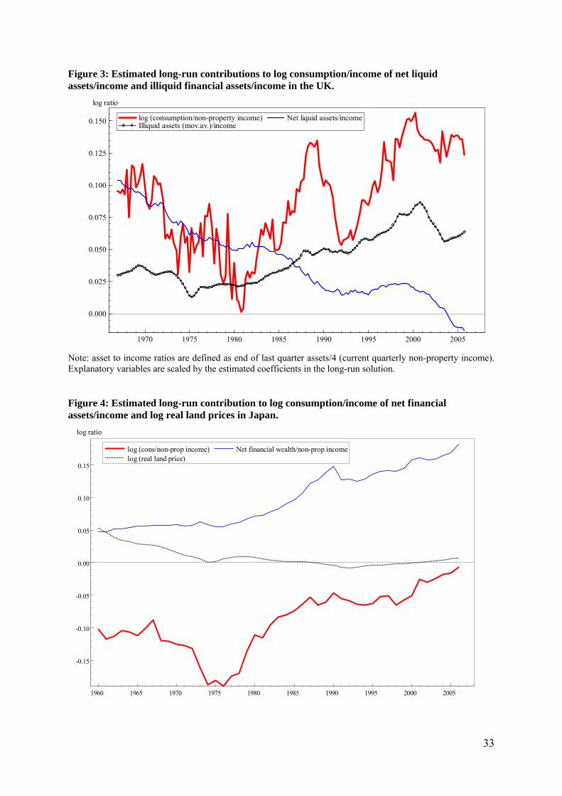
Figure 3: Estimated long-run contributions to log consumption/income of net liquid assets/income and illiquid financial assets/income in the UK.

1970 1975 1980 1985 1990 1995 2000 2005

0.000

0.025

0.050

0.075

0.100

0.125

0.150

log ratio

log (consumption/non-property income) Illiquid assets (mov.av.)/income

Net liquid assets/income

Note: asset to income ratios are defined as end of last quarter assets/4 (current quarterly non-property income). Explanatory variables are scaled by the estimated coefficients in the long-run solution. Figure 4: Estimated long-run contribution to log consumption/income of net financial assets/income and log real land prices in Japan.

1960 1965 1970 1975 1980 1985 1990 1995 2000 2005

-0.15

-0.10

-0.05

0.00

0.05

0.10

0.15

log ratio

log (cons/non-prop income) log (real land price)

Net financial wealth/non-prop income

33

Figure 5: Estimated long-run contribution to log consumption/income of real interest rate and forecast income growth in Japan.

1960 1965 1970 1975 1980 1985 1990 1995 2000 2005

-0.15

-0.10

-0.05

0.00

0.05

log ratio

Log (cons/non-prop income) forecast growth of log y

real interest rate

Figure 6: Growth of US Permanent Income.

1960 1965 1970 1975 1980 1985 1990 1995 2000 2005 2010

0.025

0.050

0.075

0.100

0.125

0.150

log ratio

fitted log ratio of permanent income to current income actual log ratio of permanent income to current income

34

Figure 7: Stabilisation of the US Consumer Credit Conditions Index Growth after its decline in the recent financial crisis.

1970 1975 1980 1985 1990 1995 2000 2005 2010

0.0

0.1

0.2

0.3

0.4

0.5

0.6

0.7

0.8

0.9

1.0index: 0-1

US Credit Conditions Index

Figure 8: The US Index of Housing Liquidity

1975 1980 1985 1990 1995 2000 2005 2010

0.1

0.2

0.3

0.4

0.5

0.6

0.7

0.8

0.9

1.0Index: 0 in 1970q1

US Index of Housing Liquidity

35

Table 1: Estimates of the UK Consumption Function for 1967 Q1 to 2005 Q4 Dependent variable = ln tcΔ (1) (2) (3) (4)

Credit Conditions Index, CCI ( )CCIoα - - 0.020

(3.5)

1ln lny c−− ( )β 0.16 (4.9)

0.23 (6.3)

0.31 (8.5)

0.33 (8.9)

Real mortgage interest rate ( )1α - - -0.03 (1.4)

-0.04 (1.5)

Change in unemployment rate 4urΔ ( )2α - - -0.56 (7.8)

-0.64 (8.6)

Forecast income growth ln typermΔ ( )3a 0.21 (4.9)

0.18 (4.4)

0.22 (5.5)

0.10 (2.4)

Forecast income growth and CCI interaction ( )3

CCIα - - - 0.15 (1.6)

Net liquid assets/income ( )1γ 0.0036 (4.8)

0.026 (4,3)

0.033 (5.6)

0.038 (5.6)

Illiquid financial assets/income ( )2γ Ditto 0.0076 (5.9)

0.0071 (5.1)

0.0061 (4.7)

Housing assets/income ( )3γ Ditto Ditto 0.0111 (5.7) -

Housing assets/income and CCI interaction ( )3

CCIγ Ditto - - 0.0106 (6.3)

Debt/income and Δ4 nominal interest rate interaction ( )2β - - -0.0029

(3.8) -0.0072

(3.1)

Debt/income, Δ4 nominal interest rate and CCI interaction ( )2

CCIβ - - - 0.0057 (1.9)

Diagnostics

Standard error x 100 0.76 0.73 0.61 0.59

Adjusted R2 0.58 0.62 0.73 0.76

Durbin Watson 1.41 1.34 1.85 1.98

P-value for no structural break 0.11 0.064 0.093 0.754

Notes: 1. The t-statistics are in parentheses. 2. The interaction effect with housing assets/income, takes the form (housing assets/income - 3.08) x CCI,

where 3.08 is the mean value of housing wealth/income for 1980-2005. 3. The estimated equation is:

( )( ) ( )

0 0 1 1 2 3 3

1 1 2 1 3 1 3 1

2 1 2 1

de-meaned

ln ln ln ln ln

[]

CCI CCIt t t t t t t t

CCIt t t t t t t t t

CCIt t t t t t t

c CCI y c r ur yperm yperm CCI

NLA y IFA y HA y HA y CCI

nr DB y nr DB y CCI

β α α α α α α

γ γ γ γ

β β

−

− − − −

− −

Δ ≈ + + − + + Δ + Δ + Δ ×

+ + + + ×

+ Δ × + Δ × ×

t

36

Table 2: Japanese Consumption Function Estimates for 1961 -2006

Dependent variable = ln cΔ (1) (2) (3) (4)

Intercept -0.055 (3.3)

-0.057 (3.6)

-0.058 (4.0)

-0.063 (4.3)

1ln lny c−− 0.356 (5.3)

0.345 (5.4)

0.347 (5.5)

0.359 (5.6)

Real interest rate (tax-adjusted) 0.346 (5.6)

0.346 (5.8)

0.350 (6.5)

0.367 (6.8)

Change in unemployment rate, urΔ -0.008 (1.6)

-0.007 (1.5)

-0.007 (1.5)

Income growth volatility -0.225 (2.4)

-0.024 (0.2)

Forecast income growth 0.367 (4.4)

0.347 (4.4)

0.348 (4.5)

0.350 (4.4)

Income growth volatility x Forecast income growth -5.666

(2.2) -6.007 (3.4)

-5.648 (3.1)

Net financial wealth-1/income 0.022 (4.1)

0.022 (4.3)

0.023 (4.5)

0.024 (4.8)

Log real land price-1 -0.014 (3.2)

-0.015 (3.5)

-0.015 (3.6)

-0.016 (4.0)

Income growth, ln yΔ 0.289 (4.1)

0.321 (4.7)

0.323 (4.8)

0.332 (4.9)

Diagnostics

Standard error x 100 0.681 0.648 0.640 0.650 Adjusted R2 0.941 0.947 0.948 0.946 Durbin Watson 2.14 2.20 2.20 2.22 AR1/MA1 (p-value) 0.621 0.386 0.417 0.396 AR2/MA2 (p-value) 0.742 0.711 0.717 0.726 Heteroscedasticity (p-value) 0.737 0.849 0.829 0.955 Chow (p-value) 0.255 0.191 0.298 0.635 RESET(p-value) 0.066 0.445 0.576 0.827

Note: The t-statistics are in parentheses.

37

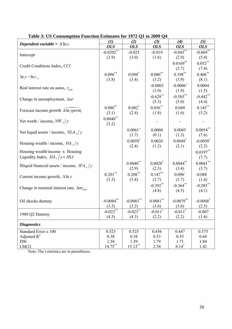
Table 3: US Consumption Function Estimates for 1972 Q1 to 2009 Q4

(1) (2) (3) (4) (5) Dependent variable = ln cΔ OLS OLS OLS OLS OLS

Intercept -0.0202**

(2.9) -0.025 (3.0)

-0.019 (1.6)

-0.043** (2.9)

-0.069** (5.4)

Credit Conditions Index, CCI 0.0169** (2.7)

0.052** (7.4)

1ln lny c−− 0.096** (3.8)

0.098* (3.4)

0.080** (3.2)

0.198** (3.9)

0.406** (8.1)

Real interest rate on autos, autor -0.0003 (1.0)

-0.0006+ (1.9)

0.0004 (1.5)

Change in unemployment, urΔ

-0.629** (5.3)

-0.585** (5.0)

-0.442** (4.4)

Forecast income growth ln typermΔ 0.080** (3.1)

0.082* (2.4)

0.056*+ (1.8)

0.049 (1.6)

0.145** (5.2)

Net worth / income, 1NW y− 0.0040** (3.2)

- - -

Net liquid assets / income, 1NLA y− 0.0061+ (1.7)

0.0004 (0.1)

0.0045 (1.3)

0.0054** (7.6)

Housing wealth / income, 1HA y− 0.0059* (2.4)

0.0026 (1.2)

0.0049* (2.1)

-0.0050* (2.2)

Housing wealth/income x Housing Liquidity Index, 1HA y HLI− × 0.0197**

(7.7)

Illiquid financial assets / income, 1IFA y− 0.0040** (2.9)

0.0028* (2.3)

0.0044** (3.4)

0.0041** (3.7)

Current income growth, ln yΔ 0.201** (3.3)

0.208** (3.4)

0.147** (2.7)

0.096+ (1.7)

-0.088 (1.6)

Change in nominal interest rate, autonrΔ -0.392** (4.8)

-0.364** (4.5)

-0.285** (4.1)

Oil shocks dummy

-0.0084** (3.3)

-0.0083**

(3.2)

0.0081**

(3.6)

-0.0079**

(3.6)

-0.0048*

(2.5)

1980 Q2 Dummy -0.023** (4.3)

-0.023** (4.3)

-0.011* (2.2)

-0.011* (2.2)

-0.007 (1.6)

Diagnostics

Standard Error x 100 0.523 0.525 0.456 0.447 0.375 Adjusted R2 0.38 0.38 0.53 0.55 0.68 DW 1.58 1.59 1.79 1.71 1.84 LM(2) 14.75** 15.13** 2.54 6.14* 1.42

Note: The t-statistics are in parentheses.

38

Appendix Table 1: US Consumption Estimates for 1972:Q1 to 2009:Q4, Lagged Income

(1) (2) (3) (4) (5) Dependent variable = ln cΔ OLS OLS OLS OLS OLS

Intercept -0.012+

(1.7) -0.016+

(1.9) -0.015 (1.9)

-0.019 (1.2)

-0.038** (2.8)

Credit Conditions Index, CCI 0.003 (0.4)

0.029** (4.4)

1 1ln lny c− −− 0.069* (2.5)

0.057+

(1.9) 0.052+ (2.1)

0.072 (1.4)

0.215** (4.6)

Real interest rate on autos, autor 0.0004 (1.2)

0.0004 (1.3)

0.0004 (1.3)

Change in unemployment, urΔ

-0.696** (5.5)

-0.694** (5.5)

-0.645** (5.6)

Forecast income growth, 1log yperm−Δ 0.066* (2.4)

0.042 (1.2)

0.030 (1.0)

0.027 (0.9)

0.073** (2.6)

Net wealth / income, 1 1NW y− − 0.0027*

(2.0) - - -

Net liquid assets / income, 1 1NLA y− − 0.0080 (2.1)

-0.0011 (0.3)

0.0019 (0.5)

0.039** (4.7)

Housing wealth / income, 1 1HA y− − 0.0030 (1.2)

0.0005 (0.2)

0.0008 (0.3)

-0.0075** (2.8)

Housing wealth/income x Housing Liquidity Index, 1 1HA y HLI− − × 0.0142**

(4.8)

Illiquid financial assets / income, 1 1IFA y− − 0.0034 (2.4)

0.0024+ (1.9)

0.0027+ (1.9)

0.0027* (2.1)

Lagged income growth, 1ln y−Δ 0.178** (3.0)

0.169** (2.8)

0.095+ (1.8)

0.089 (1.6)

0.008 (0.2)

Change in nominal interest rate, autonrΔ -0.412** (4.7)

-0.408** (4.6)

-0.353** (4.3)

Oil shocks

-0.0102** (3.8)

-0.0107**

(3.9)

0.0099**

(4.2)

-0.0100**

(4.2)

-0.0088**

(4.0)

1980 Q2 Dummy -0.028** (5.0)

-0.028** (4.9)

-0.010** (4.2)

-0.014* (2.6)

-0.012* (2.4)

Diagnostics

Standard Error x 100 0.563 0.562 0.483 0.484 0.445 Adjusted R2 0.29 0.29 0.47 0.47 0.54 DW 1.53 1.54 1.72 1.71 1.83 LM(2) 13.38** 12.47** 3.44 3.87 3.12

Note: The t-statistics are in parentheses.

39

Appendix: Constructing a U.S. Credit Conditions Index

This appendix describes the construction of a consumer credit conditions (CCI) index in

levels using U.S. data on an index of changes in bank willingness to make consumer

instalment loans. Before constructing a levels index from this relative change index, we first

adjust it for identifiable effects of interest rates and the macroeconomic outlook by estimating

an empirical model based on screening models. In such models credit standards should be

tightened when the real riskless rate rises and the macroeconomic outlook worsens (see Duca

and Garrett, 1995; and the screening model of Stiglitz and Weiss, part IV, 1981). Since the

willingness to lend index is inversely related to credit standards, these expected signs are

reversed in our empirical model of the diffusion index. We track the former by including the

lag of the first difference of the real federal funds rate (ΔRFF, the nominal funds rate minus

the year-over-year percent change in the overall PCE deflator), and the latter by the two-

quarter percent change in the index of leading economic indicators (ΔLEI2). To further

adjust for factors affecting consumer loan quality, we include the time t year-over-year

change in the delinquency rate on all consumer instalment loans at banks (Δ4DEL, American

Bankers Association).

Three variables are included to control for the impact of regulation. One is a dummy

equal to 1 in 1980:q2 when credit controls were imposed and equal to -1 when they were

lifted in 1980:q3 (DCON). The second, REGQ, tracks the degree to which Regulation Q

ceilings impinged upon banks’ ability to raise small time deposit rates (see Duca, 1996; and

Duca and Wu, 2009) and thereby raised banks’ shadow cost of raising loanable funds

(Regulation Q was binding during an era before the loan sales and mortgage-backed

securities markets were deep). The third regulatory variable is MMDA, equal to 1 in 1982:q4

and 1983:q1, and 0 otherwise, for banks being allowed to offer adjustable interest rate

savings deposits (money market deposit accounts) that were a close substitute for money

market mutual funds (MMMFs). MMDA controls for the re-intermediation effect of

households shifting funds into MMDAs partly from MMMFs and nonM2 assets, which

increased the supply of funds to banks, and induced an increase in their willingness to make

consumer loans. MMDA was used to control for regulatory effects in earlier Federal Reserve

Board money demand models (Duca, 2000). After Regulation Q was lifted, the interbank

funding market increasingly became a marginal source of loanable funds, with the three-

month LIBOR normally exceeding the expected 3-month average federal funds rate by about

10-12 basis points. However, as fears of bank portfolio losses and liquidity premiums soared

40

41

during the current financial crisis, so did these spreads, which raised one marginal cost of

funding loans. To control for this, we include a dummy (LEHMAN=1 in 2008:q4) for the

failure of Lehman (which was after the 2008:q3 Fed survey) and the spread between the 3-

month LIBOR and 3-month Treasury Bill rates (LIBOR3). [The three-month T-bill rate,

which tracks the expected average federal funds rate over the next three months, was used

instead of the 3-month OIS rate which is unavailable before 2003.]

Estimating from 1966:q3 to 2009:q3 with an AR(1) correction yields:

CR = 14.36 – 3.48*ΔRFFt

** + 1.09*ΔLEI2t

** - 12.49*Δ4DELt ** + 26.72*MMDAt

** (4.30) (-4.69) (4.48) (-2.86) (3.72)

- 2.47* REG t

* + 46.89 *DCONt** - 4.58* LIBOR3t

** - 19.98*LEHMANt **

(-2.16) (-10.33) (-2.75) (-2.63)

where t-statistics are in parentheses, R2 = 0.805, AR(1) = 0.743** (t stat.: 13.93), standard

error = 9.04, LM(2) = 0.64, and Q(24) = 18.91. The coefficients have the anticipated signs

and are all significant. It is reassuring that in regressions not shown, the model coefficients

hardly change in magnitude, especially the coefficient on the LIBOR spread, in samples that

pre-date the initial effects of the financial crisis in August 2007 (when the LIBOR spreads

began widening) and the peak effects to date of the crisis on money market and interbank

lending conditions during late 2008.

We subtract the estimated impact of changes in the real federal funds rate, leading

economic indicators, and the delinquency rate to remove normal business cycle and interest

rate effects, leaving the impact of regulations, Lehman’s failure, unusual credit (LIBOR)

frictions, and unexplained movements in the adjusted diffusion index (CRAdj). We transform

CRAdj into a levels index using the ratio of the average growth rate of real per capita

consumer loan extensions (available 1966-1982:q4) divided by real per capital nonproperty

income to the average of CRAdj over this interval (.007390/7.598375). Setting 1966:q2 =

100, the levels index evolves as CCIUt = CCIUt-1*[1+(.000391*CRAdj)]. This multiplicative

aggregation is consistent with the Senior Loan Officer Opinion Survey question asking

whether a bank’s willingness to make consumer loans was much more, somewhat more,

unchanged, somewhat less, or much less compared to three months earlier. We scale CCIU

by subtracting 100 from it to equal 0 in 1966:q2 and dividing all values (CCIU-100) by the

peak value of (CCIU-100) in 2007:q3. The resulting index CCI mainly ranges between 0 and

1, dips below 0 in 1966:q3-q4, and peaks at 1 in 2007:3. It rises greatly during the 1980s, and

increases over 2004-06, before falling back to 2003 levels.