Creating and Capturing Value in Repeated Exchange ...apps.olin.wustl.edu/faculty/elfenbein/ElfenbeinZengerSecondParadox.pdfCreating and Capturing Value in Repeated Exchange Relationships:

Creating and Capturing Value in Repeated Exchange Relationships:

The Second Paradox of Embeddedness

Daniel W. Elfenbein

Olin Business School

Washington University in St. Louis

One Brookings Drive

St. Louis, MO 63130-4899

Phone: (314) 935-8028

Fax: (314) 935-6359

[email protected]

and

Todd R. Zenger

David Eccles School of Business

University of Utah

Salt Lake City, UT 84112

Phone: (801) 585-3981

[email protected]

forthcoming Organization Science

April 2017

Acknowledgements: The Boeing Center for Technology, Information, and Manufacturing provided

generous research support for this project. We thank Joel Baum, Jeff Dyer, Ranjay Gulati, Olav Sorenson

and seminar participants at Bocconi University, Massachusetts Institute of Technology, University of

Amsterdam, University of Illinois, and University of Michigan, the University of Utah/BYU Winter

Strategy Conference, the Atlanta Competitive Advantage Conference, and the Sumantra Ghoshal

Conference at London Business School, INFORMS, and ISNIE, for helpful comments. We also thank

Dan Douglass and Tracy Smith Clyburn for many helpful conversations, and we thank Ellen Wen, Nina

Noll, Jon D’Antonio, Chase Zenger, and Andrew Zenger for research assistance in assembling these data.

Creating and Capturing Value in Repeated Exchange Relationships:

The Second Paradox of Embeddedness

April 2017

ABSTRACT

Prior empirical studies suggest repeated exchange develops increasing value in buyer-supplier

relationships. A first order implication of this finding is that buyers will concentrate exchange

among a relatively small number of suppliers to generate maximum value in relationships.

However, buyers are equally concerned with value capture. By distributing rather than

concentrating exchange, buyers may position themselves to capture more of the value created,

leaving buyers potentially conflicted concerning the choice. We label this dynamic the second

paradox of embeddedness, distinguishing it from Uzzi’s (1997) paradox driven by technological

uncertainty. By examining the procurement activities of a large, diversified manufacturing

company, we then test for supplier and buyer behavior consistent with the conditions that give

rise to the second paradox and behaviors that result from it.

Keywords: relational capital, buyer-supplier relationships, value appropriation, procurement,

portfolio of relationships

1

1. INTRODUCTION

A broad scholarly literature argues that repeated exchange between firms improves the efficiency

of exchange by mitigating ex post opportunism and fostering value-creating adaptation (e.g., Granovetter

1985, Williamson 1996, Dyer 1997, MacLeod 2007). Repeated exchange develops trust (Zaheer,

McEvily, and Perrone 1998, Jeffries and Reed 2000), inter-organizational routines (Dyer and Singh

1998), social connections between individuals in each firm (Levinthal and Fichman 1988, Uzzi 1999),

and heightened expectations of relationship continuity (Parkhe 1993). Together, these factors expand the

value created in exchange – value that dynamically increases with evolving exchange histories (Kale,

Perlmutter, and Singh 2000, Gulati and Stych 2008). Over the past two decades, the value-creating

potential of such “embedded” inter-organizational relationships has been well documented empirically

(e.g., Gulati 1995, Zollo, Reuer, and Singh 2002, Dyer and Chu 2003, Gulati and Nickerson 2008),

including direct evidence that economic value produced by relationships increases with exchange history

within a dyad (Elfenbein and Zenger 2014). A clear first-order implication of the build-up of relationship

value through repeated exchange is for buyers to focus their exchange, developing increasingly deep

relationships with a limited set of capable suppliers, in order to maximize value creation.

At the same time, scholars have highlighted a number of hazards associated with relationships. If

changing exchange conditions or production technology undermine current suppliers’ advantages,

concentrating exchange and developing only a handful of these deep, socially embedded exchange

relations may leave buyers “stuck” in suboptimal long term relationships (Blau; 1964; Uzzi 1997; Afuah,

2000). Moreover, interpersonal affinity that develops through repeated exchange may also shape (or

distort) the selection of exchange partners. As Blau (1964) articulates rather simply: “Strong attachments

prevent individuals from exploring alternative opportunities.” The result is a “dark side” to relationships,

or an embeddedness paradox (Uzzi 1997) where buyers benefit from relationships in the present, but at

the cost of neglecting to identify or to choose a set of suppliers better suited to future needs.

Yet, even in the absence of these traditionally cited “dark side” problems of deep (and potentially

exclusive) relationships, concentrating exchange in the hands of a few may not be value maximizing for

2

the buyer. This stems from two fundamental tensions that have been largely, if not completely, ignored in

the literature on relationships. First, a buyer’s choice of supplier in the present can either increase the

maximum relationship value available for future appropriation or increase the minimum it is assured of

appropriating, but not both. Second, a buyer’s choice of supplier reveals information to the supplier about

the value the buyer assigns to relationships, making it easier for the supplier to claim a portion of the

value that is “up for grabs” in the future. In the spirit of the prior literature, we denote these tensions as

the “second paradox of embeddedness.” The focus of this paper, then, is to define the tensions that

comprise the second paradox and highlight their boundary conditions. We also provide evidence

consistent with their existence in an empirical context in which relationships create value, but the

traditional “dark side” challenges have been mitigated by a routinized process of extensive search for and

screening of potential new suppliers and by a transparent, de-socialized supplier selection process that

minimizes distortions due to interpersonal affinity.

Our main theoretical argument builds on the value-based strategy literature (Brandenburger and

Stuart 1996, Lippman and Rumelt 2003, MacDonald and Ryall 2004, Stuart 2015) that focuses on how a

firm’s added value constrains its capacity to capture value as it engages competitively or cooperatively

with other firms in generating value. Drawing inspiration from bi-form games (Brandenburger and Stuart

2007, Bennett 2013), we describe how the future added value of suppliers changes as a consequence of

the buyer’s current decision and we demonstrate the dilemma the buyer faces. In simple terms, the

buyer’s dilemma is between growing the minimum appropriable value by distributing exchange and

growing the maximum appropriable value by focusing exchange. Focus creates deep relationships and

larger value with a single (or few) seller(s), but leaves the division of this greater value between buyer

and seller uncertain. Distribution restricts the maximum value created by relationships, but also

diminishes the uniqueness (i.e., added value) of any given supplier’s relational history, and thereby

elevates the value that a buyer can appropriate with certainty. We further describe how this dilemma is

also shaped by buyers’ beliefs about suppliers’ future strategies for claiming value that is “up for grabs.”

3

Our empirical analysis examines the procurement efforts of a large manufacturing corporation

that performs a significant portion of its parts sourcing via Internet-based reverse (procurement) auctions.1

As the preceding discussion suggests, we potentially face a conceptual challenge in interpreting any

empirical results as multiple theories predict the same behavior. In particular, both the first and our

second paradox suggest a buyer may distribute exchange across suppliers rather than concentrate it. We

therefore select an empirical setting where the buyer’s selection of suppliers is unlikely to be shaped by

the challenges inherent in the first paradox of embeddedness, leaving us more confident that the behavior

we observe reflects our theorized second paradox. This setting also provides fine-grained detail about

final supplier prices of bids both accepted and rejected as well as extensive detail about exchange history,

providing us with the rare capacity to examine both the total value the buyer associates with exchange

history and suppliers’ attempts to appropriate it.

In this empirical setting, the buyer we examine typically awards three-year supply contracts to

one of several bidders who compete for the contract. Bidding for supply contracts is strictly limited to

those suppliers pre-qualified by a dedicated team of supply chain professionals as possessing a capacity to

manufacture and reliably deliver that specific set of items. All supplier bids, supplier and product

characteristics, and the buyer’s choices are observable.

While the parts procured through these auctions are predictably more standardized than those

manufactured internally, important exchange hazards remain. Although all suppliers are prequalified as

capable of high quality production and reliable delivery, such performance over the lifetime of the

agreement is a supplier choice. In addition, some exchange specific investments may be required that, if

ignored, compromise quality or reliable delivery. In this context, repeated exchange can generate

relationships that remedy these exchange hazards, facilitating joint problem solving and cooperative

behavior that generates value. Indeed, previous research in this empirical context demonstrates that a

history of prior exchange with a supplier raises the buyer’s willingness-to-pay (see Elfenbein and Zenger,

1 This is the same empirical context examined in Elfenbein and Zenger (2014). Whereas that paper documented the

emergence of relational capital through repeated exchange, this paper focuses on the division of relationship value

between buyer and supplier and how this constrains the buyer’s choice of suppliers.

4

2014), creating what others have termed as valuable “relational capital” (Kale, Perlmutter, and Singh

2000).2

Although the buyer in these auctions may choose any supplier that bids, the choice commits the

buyer to the bid price. Thus, bid prices represent suppliers’ proposed division of value, including the

value embedded in exchange history. Our ability to examine the array of prices offered from these

suppliers, each with a unique relationship history, provides a window into the dynamics of buyer and

supplier efforts to create and capture value in relationships. We use this unique empirical setting to test

for evidence consistent with hypotheses derived from our theoretical articulation of the second paradox of

embeddedness. Our results support our hypotheses. We view our theory and results as contributing to the

literature on buyer-supplier relationships by offering an alternative mechanism through which firms forgo

the benefits of deep relationships in favor of shallower ones. We do not claim primacy of this mechanism

over others, but we do provide evidence consistent with its existence in an economically important

setting. Additionally, we contribute to a small, but growing set of empirical studies on value appropriation

in inter-firm relationships (e.g., Lavie 2007, Chatain 2011, Adegbesan and Higgins 2011, Grennan 2012),

and broader theoretical investigations of how value creation and value appropriation concerns shape

performance differences in and across firms over time (e.g., Ryall and Sorenson 2007, Chatain and

Zemsky 2007, Chatain and Zemsky 2011, Bennett 2013, Obloj and Zemsky 2015).

2. THEORY AND PREDICTIONS

Repeated exchange, relational capital, and buyer willingness-to-pay

A central tenet of modern economic theory is that writing and enforcing contracts that completely

specify each party’s obligations in all states of the world is rarely possible (Williamson 1975). Many of

2 In many settings there may be symmetry to the value embedded in an exchange relationship. A history of repeated

exchange may not only enhance the buyer’s willingness to pay by enhancing coordination and problem solving

capacity and reducing fears of opportunism, as discussed below, but may also lower costs for the supplier, enabling

such suppliers to offer lower prices. Due to the nature of the rather simple parts we examine, as well as data

constraints (i.e. we only observe a suppliers’ prices to a single buyer) and the fact any such symmetry would only

bias us against finding any significant results, we have chosen to theoretically and empirically focus on the value to

the buyer of an exchange history.

5

the activities that generate (or destroy) value within an exchange are simply non-contractible (Hart 1994).

They require adaptation and real time problem solving. Hence, performance on these dimensions must

instead be promoted through other means, such as bringing the transactions inside the firm (Williamson

1985), or as discussed below, through repeated exchange relations.

As the frequently cited alternative to integration, repeated exchange relationships can improve

performance along non-contractible dimensions of exchange through several related mechanisms.

Repeated exchange promotes embedded social relationships, social norms, and personal attachments

(Dore 1983, Gerlach 1992; Macneil 1978, Bradach and Eccles 1982, Granovetter 1985) that reduce fears

of opportunistic behavior (Zaheer, McEvily, and Perrone 1998, Dyer and Chu 2003, Gulati and Nickerson

2008, Puranam and Vanneste 2009, Bradach and Eccles, 1989). Repeated exchange also fosters

information exchange, norms of flexibility, and joint problem solving (Uzzi 1997, Dyer and Singh 1998,

Poppo and Zenger 2002), collectively combining to support the adaptation critical to effective exchange.

In aggregate, deeper histories of repeated exchange with suppliers enhance a buyer’s confidence that the

suppliers, when faced with competing interests (i.e. the interests of others buyers), will possess both the

will and means to both fulfill contract terms and to respond flexibly and effectively to unexpected

circumstances; this raises the buyer’s willingness-to-pay by diminishing costly inventory holding and

reducing expected costs of adaptation or re-negotiation should unexpected circumstances arise.3 In

summary, a broad set of arguments all support a conclusion that a history of repeated exchange generates

a valuable asset (Nahapiet and Ghoshal 1998) – one that supports adaptation and problem solving, and

deters opportunistic behavior.4

Prior empirical analysis is also consistent with a conclusion that value accumulates with increased

relationship history. A meta-analysis of 39 studies documents a positive and significant association

between relationship duration and trust (Vanneste, Puranam and Kletschmer 2014). Other work suggests

3 Gubler (2015) shows that relationships are associated with better performance even in the absence of the shadow

of the future, which he attributes to more effective information sharing and higher motivation. 4 Some scholars have referred to the idiosyncratic value that emerges through these interactions as “relational rents”

(Dyer and Singh 1998, Lavie 2006).

6

that costs fall as a consequence of repeated dyadic interaction between contractors and subcontractors (Gil

and Marion 2013). More directly, our own prior study in this empirical setting reveals a buyer whose

willingness to pay for a relationship is strongly shaped by the level and duration of repeated exchange;

these relationships are more highly valued by the buyer when exchanges are subject to greater hazards,

specifically when suppliers are required to make co-specialized investments (Elfenbein and Zenger 2014).

Considered in isolation, this evidence that relational capital accumulates through repeated

exchange should cause a buyer’s supply network to become more concentrated over time, especially for

transactions subject to exchange hazards. A supplier with greater relational capital is simply more

attractive to a buyer and more likely to be chosen, ceteris paribus, leading to focused rather than

distributed exchange. However, as we develop and test below, the desire to optimize the value created

and captured leads to more complex predictions about buyer behavior. In particular, we argue that the

buyer faces a dilemma in choosing between further increasing value in the most valuable exchange

relationships and instead developing a more diverse set of relationships that ensure a greater minimum

level of value appropriation. We label this phenomenon the “second paradox of embeddedness,” articulate

the conditions under which it can emerge, and provide evidence of behavior consistent with its influence

and presence.

Sequential selection of suppliers and appropriation of relationship value

When valuable relational capital accumulates as a function of repeated exchange, a buyer’s

choice of supplier in the present not only affects the current stream of relational rents it receives, but also

the amount of future relational value available to divide between buyer and suppliers and the likely future

division of that value. In this section, we develop a simple model to illustrate the paradoxical nature of the

buyer’s choice and demonstrate how value creation and value appropriation dynamics affect it.5,6

5 We seek not to create a comprehensive model to predict the buyer’s decisions, but rather to show the main features

of the decision-making process that generate tension and, thereby, to identify the necessary conditions for observing

a paradox, if it exists.

7

We consider a two-period setting in which a buyer chooses an exclusive supplier in each period

for an input it cannot produce itself. For simplicity, we focus on a choice between two potential suppliers,

both pre-screened to possess identical production capabilities and thus a capacity to deliver the same

gross contractible value, v, if chosen. Further, we assume that it is prohibitively costly to write a contract

that covers both periods, perhaps because the specifications for parts needed in period 2 are unknown at

the beginning of period 1.7

Following the discussion above, a supplier will be expected to deliver (non-contractible) value

that is a positively increasing function of its relationship history with the buyer. We denote this prior

exchange history between the buyer and the supplier as h and the value associated with this history as

V(h), with V(0) = 0 and 𝜕𝑉

𝜕ℎ > 0. The function V(h) reflects the value to the buyer of relational capital. 8

Since we are interested in the conditions that lead a buyer to distribute rather than concentrate

exchange, we focus on the case in which one potential supplier, labeled the “incumbent”, has a history of

prior exchange, h > 0, and the second potential supplier, the “new supplier”, has no prior history with the

buyer, i.e., h = 0.9 In period 1, then, choosing the incumbent supplier generates gross value v + V(h),

whereas choosing the new supplier only generates gross value v.

Because relational capital accumulates with exchange, the buyer’s choice of supplier in period 1

affects the relational capital held with that supplier in future periods. We designate the increase in

exchange history generated during period 1 production as . For simplicity in the discussion that follows,

we assume that h > ; however, our main results do not depend on this assumption. If the incumbent is

chosen in both periods, then the gross (contractible and non-contractible) value delivered to the buyer will

be 2v + V(h) + V(h+). By contrast, choosing the incumbent in one period and the new supplier in

6 Board (2011) develops a theoretical model investigating similar issues, in which the central tension results from a

tradeoff between exploiting the gains from trade in the present transaction and developing (costly) new

relationships. 7 We ignore discounting across the periods, as it does not materially affect the analysis, though our assumption of

two periods is a stylized representation of more complex inter-temporal phenomenon. 8 Conceptually, we think of relational capital as being an increasing function of exchange history, e.g., R(h), and the

value of relational capital, as being a function of relational capital, i.e., V(R(h)). For simplicity, we suppress the

function R() from the discussion below as it does not affect our analysis in any way. 9 The analysis that follows is robust to a variety of alternative and more general assumptions.

8

another yields 2v + V(h).10 Selecting the new supplier in both periods yields 2v + V(). Intuitively, then,

it follows that choosing the incumbent supplier in both periods maximizes the total value created.

Ignoring issues of value capture, the greater non-contractible value available for appropriation makes

choosing the incumbent more attractive for the buyer, ceteris paribus.

Value created, however, is quite distinct from value captured. To examine value appropriation,

we draw upon the value-based business strategy approach of Brandenburger and Stuart (1996) and

MacDonald and Ryall (2004).11 The key proposition of this approach is that no player may appropriate

more than its “added value” – defined as the loss in total value that can be created when that player is

removed from the economic system.12 In this literature, each player’s contribution to total value created

acts as a constraint on the division of value, but may not determine it completely.13 Given our

assumptions (in particular that both suppliers are known to be able to produce contractible value v), added

value for suppliers in this setting comes entirely from differences in relationship histories. In period 1,

then, the added value of the incumbent and new supplier are V(h) and 0, respectively.

The added value of each player in period 2, however, depends on the buyer’s choice of supplier in

period 1. Table 1 below illustrates this and shows how the period 1 choice, in turn, affects the minimum

and maximum value that can be appropriated by the buyer in period 2. While the buyer is guaranteed

contractible value, v, in period 2 regardless of choice, selecting the incumbent supplier in period 1

increases the maximum value the buyer can receive to v + V(h + ); however, selecting the incumbent

leaves the minimum value it can appropriate unchanged at v. By contrast, choosing the new supplier in

10 The analysis is also robust to allowing the incumbent’s relational capital to depreciate between periods if it is not

selected. This might be akin to decreasing motivation due to losing the period 1 contract. Ceteris paribus, such an

assumption would lead to greater concentration of exchange among a small set of suppliers. 11 While we draw inspiration from bi-form games (Brandenburger and Stuart 2007, Bennett 2013), we depart from it

in some important ways in order to match our theoretical development more closely to our setting. In particular, in

our setting final prices are formed via reverse auctions, leading us to modify the depiction of bargaining ability

(referred to in bi-form games with the parameter ). 12 This results from the fact that, were a player to appropriate more than he ‘brings to the table’ that other players

would be better off cutting that player out and transacting among themselves. 13 Although the standard assumptions of this literature of full information and unrestricted bargaining are not

technically met in this setting, the fact that the buyer has enough information to form expectations about the value of

both suppliers and can (and will) exclude a party that seeks to appropriate more than it is worth are sufficient for the

standard results about added value to apply.

9

period 1 raises the minimum value that the buyer is guaranteed to capture in period 2 from v to v + V(),

while leaving the maximum value the buyer can capture in period 2 unchanged at v + V(h).14 This

tradeoff generates a paradox – for the buyer, choosing the incumbent can be both better and worse for

capturing value from relationships in the future.

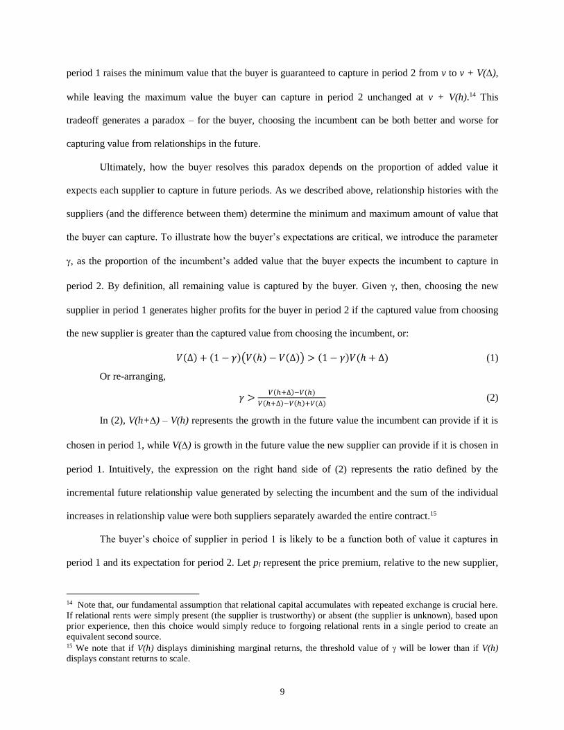
Ultimately, how the buyer resolves this paradox depends on the proportion of added value it

expects each supplier to capture in future periods. As we described above, relationship histories with the

suppliers (and the difference between them) determine the minimum and maximum amount of value that

the buyer can capture. To illustrate how the buyer’s expectations are critical, we introduce the parameter

, as the proportion of the incumbent’s added value that the buyer expects the incumbent to capture in

period 2. By definition, all remaining value is captured by the buyer. Given , then, choosing the new

supplier in period 1 generates higher profits for the buyer in period 2 if the captured value from choosing

the new supplier is greater than the captured value from choosing the incumbent, or:

𝑉(∆) + (1 − 𝛾)(𝑉(ℎ) − 𝑉(∆)) > (1 − 𝛾)𝑉(ℎ + ∆) (1)

Or re-arranging,

𝛾 >𝑉(ℎ+∆)−𝑉(ℎ)

𝑉(ℎ+∆)−𝑉(ℎ)+𝑉(∆) (2)

In (2), V(h+) – V(h) represents the growth in the future value the incumbent can provide if it is

chosen in period 1, while V() is growth in the future value the new supplier can provide if it is chosen in

period 1. Intuitively, the expression on the right hand side of (2) represents the ratio defined by the

incremental future relationship value generated by selecting the incumbent and the sum of the individual

increases in relationship value were both suppliers separately awarded the entire contract.15

The buyer’s choice of supplier in period 1 is likely to be a function both of value it captures in

period 1 and its expectation for period 2. Let pI represent the price premium, relative to the new supplier,

14 Note that, our fundamental assumption that relational capital accumulates with repeated exchange is crucial here.

If relational rents were simply present (the supplier is trustworthy) or absent (the supplier is unknown), based upon

prior experience, then this choice would simply reduce to forgoing relational rents in a single period to create an

equivalent second source. 15 We note that if V(h) displays diminishing marginal returns, the threshold value of will be lower than if V(h)

displays constant returns to scale.

10

demanded by the incumbent in period 1.16 Then the expected total two-period profits from choosing the

new supplier in period 1 are greater if:

𝑉(∆) + (1 − 𝛾)(𝑉(ℎ) − 𝑉(∆)) > 𝑉(ℎ) − 𝑝𝐼 + (1 − 𝛾)𝑉(ℎ + ∆) (3)

Re-arranging terms yields the critical value of above which, the buyer prefers to choose the new

supplier in period 1:

𝛾 >𝑉(ℎ+∆)−𝑝𝐼

𝑉(ℎ+∆)−𝑉(ℎ)+𝑉(∆) (4)

Inequality (4) indicates that the buyer’s optimal choice in period 1 depends on the price premium

the incumbent seeks, i.e., pI, and the buyer’s conjecture about the proportion of added value the

incumbent will successfully capture in the period 2, i.e., .17

Supplier value appropriation, the 2nd paradox of embeddedness, and the buyer’s response

While our model is stylized along a number of dimensions, it highlights the tension that a buyer

faces in managing value creation and value capture through the selection of suppliers and development of

relationships. The buyer’s beliefs about the share of future added value that suppliers will capture ()

critically shapes its decision to concentrate relationships in the hands of a few suppliers (akin to choosing

the incumbent in the discussion above) or distribute contracts to many. Moreover, our model shows that a

paradox exists only if the true proportion of added value captured by suppliers is sufficiently high.

We argue that the buyer generates predictions about based on the supplier behavior that it

observes.18 This has several empirical implications. First, if the buyer observes that incumbent suppliers

16 In our setting, prices are set via reverse auction, and this price premium is known to the buyer at the time of

choosing the supplier for period 1. In principle, pI can take on any value. An alternative theoretical approach – in

which unrestricted bargaining takes place in both periods – leads to a similar formulation in which the decision to

choose the new supplier in the first period depends on beliefs about value appropriation in the second period. This

alternative approach yields theoretical predictions that are consistent with all of the hypotheses in the next section. 17 As described above, we assume that the length of the supply contracts has been chosen optimally based upon

considerations outside our model. Since neither supplier is able to commit to a price in the second period – nor is the

buyer able to commit to choosing a particular supplier in the second period – the buyer’s decision and the existence

of our 2nd paradox of embeddedness then turns on buyers’ conjectures about . 18 Alternatively, the buyer could, at least in principal, use a game theoretic approach to generate predictions about .

Doing so in practice, however, would require extensive information about supplier’s opportunity costs, their

11

do not seek to appropriate value from relational capital, then we should observe the buyer concentrating

relational capital in the hands of few (i.e., the incumbents in the discussion above), raising the asymmetry

of relational capital. Under these conditions, the buyer faces no paradox.19 The second paradox arises

when incumbent suppliers do seek to appropriate significant value from relational capital by requesting

higher final prices. Relatedly, if, as our model implicitly assumes, incumbent suppliers moderate the

proportion of relationship value they seek when they compete against other suppliers that also possess

relational capital with the buyer, then reducing asymmetries between suppliers by distributing exchange

leads to greater value capture for the buyer.

Second, if the buyer observes that the proportion of relationship value incumbents seek increases

as they win more contracts, then buyers are also likely to more evenly distribute relational capital. This

sort of ‘value capture creep’ could be generated if suppliers are initially uncertain about the added value

of their relationships – either because there is asymmetric information about its value to the buyer (i.e.,

the buyer knows it but the suppliers do not) or because the supplier lacks accurate knowledge of its rivals’

exchange history – and follow a Bayesian updating process, revising upward estimates of their

relationship added value and their capacity to appropriate it after contract wins, and reducing them after

contract losses. Clearly, if the buyer’s expectation of future added value captured by the leading

supplier, is increasing with the supplier’s current contract wins, condition (4) is more likely to hold.

In summary, under these conditions, discussed above, we expect the second paradox of

embeddedness to be manifest, and expect buyers to respond by distributing exchange rather than solely

exchanging with incumbents. To guide our empirical analysis, we make predictions about the type of

supplier behavior that is likely to lead to the paradox, and then conditional on observing the predicted

discount rates, suppliers’ expectations about future transactional opportunities, as well as a precise specification of

the price-setting processes. 19 This could occur for several reasons. Suppliers might not recognize that relational capital generates value for the

buyer and increases its willingness-to-pay. Suppliers may recognize that relational capital generates value for the

buyer, but not be fully aware of the relational capital possessed by rivals or the value the buyer assigns to relational

capital and may, therefore, negotiate (or bid) conservatively. Third, incumbent suppliers might negotiate (or bid)

conservatively, with the intention of benefitting from continuity through eliminating switch-over costs or by making

other specific investments to reduce the cost to serve the buyer.

12

supplier behavior, we hypothesize how the buyer should respond. In particular, consistent with suppliers’

effort to capture a portion of their relational capital with the buyer, we predict:

H1a: The prices suppliers seek will be increasing in their prior exchange history with the buyer.

H1b: The presence of rivals with prior exchange history with the buyer, and the magnitude of

rival bidders’ exchange history, will reduce the rate at which incumbent suppliers’ own

relationship history with the buyer leads to increases in requested prices.

Further, if, as noted above, suppliers are uncertain about the true value buyers assign to relational

capital then we would expect to see suppliers update their estimates of this value as they win and lose

contracts with the buyer over time. Consistent with asymmetric information between buyer and supplier

about the value assigned to prior exchange history and suppliers updating beliefs about their relationship

added value based upon buyer decisions, we predict and test the following condition that, if present,

deepens the paradox:

H2: The price premiums sought by suppliers with prior exchange histories should increase

following winning bids and should decrease following losing bids.

If the first set of hypotheses (H1a and H1b) is supported, then a necessary condition for the

existence of the paradox is satisfied. If additionally, H2 is supported, the paradox becomes even more

likely. Although neither is a sufficient condition, we make the following prediction about the buyer’s

response:

H3: If H1 and H2 are supported, then the buyer’s awards will tend to increase the symmetry of

relational capital among suppliers, leading to a reduced concentration of relational capital in the

supplier base; otherwise the buyer’s awards should focus relational capital among suppliers.

Buyer efforts to shape seller appropriation efforts

The buyer may not simply react to suppliers’ value appropriation behavior, but instead seek to

shape it. Inequality (3) compares the expected total (two-period) profits from choosing the new supplier in

the first period with the expected profits from choosing the incumbent. We note that both sides of this

inequality are decreasing in , indicating that reductions in the proportion of relationship added value

appropriated by suppliers are valuable to the buyer entirely independent of its choice in the first period.

13

One mechanism through which the buyer may shape sellers’ value appropriation attempts is to

restrict sellers’ capacity to learn about the the value it assigns to relationships (i.e. the function V), causing

sellers to either underestimate or be more uncertain about this value. In response to increased uncertainty

about this value function, a risk averse supplier may correspondingly decrease its bid prices to increase its

perceived odds of winning a contract. Moreover, a buyer may wish to shape sellers’ expectations about

the division of added value that it is willing to accept. As in a repeated ultimatum game, the buyer may

seek to develop a reputation for only accepting low prices (Roth 1995, Nowak, Page, and Sigmund 2000).

The buyer may also resort to deceptive tactics to influence sellers’ assessments of its willingness-to-

accept (Boles, Croson, and Murnighan 2000), or may engage in “signal jamming” by adding noise to the

selection process to make the bidders inference problem more difficult (Fudenberg and Tirole 1986; Stein

1989). In our setting, the buyer may find it strategically advantageous to keep the seller guessing as to the

value assigned or simply lower the seller’s estimate of the value assigned.

Viewed from an alternative perspective, consistent choices based upon (4) should enable

incumbent suppliers ultimately to discover and then submit prices just under levels that would cause the

buyer to switch. To prevent this, in selecting among bids, the buyer may vary the weight it assigns to

relational capital, making more difficult the supplier’s task of inferring the buyer’s value function and the

share it is willing to accept. This predicted behavior is an additional manifestation of the paradox, insofar

as it offers a mechanism through which the buyer’s choice of an “inferior” supplier in the present may

make the buyer better off in the future. This logic suggests the following hypothesis regarding buyer

behavior:

H4: To prevent sellers from accurately inferring its willingness-to-pay for a history of exchange,

the buyer will avoid appearing to assign a consistent value to this history over time.

3. EMPIRICAL SETTING

We test our theoretical predictions using rather unique data assembled from the procurement

operations of a large, global diversified manufacturing company with headquarters in the Mid-Western

14

United States. We refer to this company as Buyco. Beginning in 2000, Buyco relied increasingly on

Internet-enabled reverse auctions to procure intermediate parts for use in manufacturing. The use of

Internet-enabled procurement auctions was a key strategic initiative at Buyco aimed at reducing overall

manufacturing costs. These procurement auctions enabled greater direct competition between suppliers

and also elevated the transparency of purchasing decisions, thereby reducing potential distortions to prices

shaped by the presence of personal relationships. We highlight the most significant aspects of this

procurement process in the ensuing discussion; we discuss the setting in greater detail in Elfenbein and

Zenger (2014).

A procurement auction, or competitive bid event (CBE), as Buyco labeled it, began with the

identification of a bundle of items which Buyco believed could be efficiently provided by a single

supplier. A given CBE could include a single bundle of products or could include several bundles. Buyco

typically restricted the bundles in a CBE to a single narrowly-defined commodity category – e.g., plastic

parts, stamped parts, or fasteners – taking advantage of the commodity-specific knowledge of its

procurement staff.

After identifying a common bundle or set of bundles, Buyco scheduled a competitive bid event.

Buyco used the event to solicit bids from invited suppliers for long-term contracts to deliver the parts (the

median contract length was three years). Invited suppliers’ bids became final at the end of the event;

further negotiations following the conclusion of bidding was prohibited. Buyco, however, was not

restricted to picking the supplier who provided the lowest bid.20 For each auction, we observe a menu of

bidders and prices from which Buyco selects a single bidder.

Critically, Buyco limited participation in the CBE to bidders that had been pre-qualified. A

dedicated team of supply chain specialists travelled globally to identify and inspect potential bidders.

These procurement professionals assessed suppliers’ capability and ensured that only those with the

capability to produce and deliver the expected quality and quantity received invitations to participate.

20 Buyco, however, did take precautions to ensure that the decision makers avoided overpaying for familiar

suppliers. As one procurement manager commented, division managers would “need to have a good explanation

when not awarding to the low bidder” and “anything that is not quantifiable [is] looked at very critically.”

15

Bidders frequently were qualified to bid on some, but not all, of the contracts in the CBE. According to

standard documents provided by Buyco to potential bidders,

“[Buyco] has rigorously reviewed supplier information to determine which suppliers are

qualified to participate in this bid opportunity. Qualified suppliers have been invited to bid on a

[bundle] by [bundle] basis. [Buyco], working with [auctioneer], will grant [bundle]-level access

to suppliers.”

Thus, prior to the initiation of a bid event, two drivers of the standard embeddedness paradox (Uzzi,

1997) – uncertainty about requisite capability of suppliers and development of a set of capable

alternatives – had been addressed.

While the extensive pre-qualification process excludes bidders who do not possess the

manufacturing capabilities to produce inputs of sufficient quality, the process does not resolve uncertainty

about the potential for supplier opportunism over the duration of the supply contract. Given this extensive

pre-qualification, and careful corporate scrutiny of all selections not consistent with lowest price,

differences in bid prices across suppliers likely reflect bidders’ beliefs about value in relationships and the

bidder’s efforts to capture this value, rather than differences in production quality above and beyond the

stipulated standard that have no economic benefit to Buyco, as well as (unobservable) differences in their

opportunity costs.

4. DATA

The sample

To construct the data, we selected CBEs performed during an 18 month period covering April

2005 to September 2006. This period corresponded to the beginning of a transition to a new application

service provider that supplied technology and other support for the auctions. We limited our attention to

economically important CBEs (more than $40,000 in expected annual spending) for items used directly in

the manufacturing process. All auctions for indirect, i.e., overhead expenses, were omitted. This yielded

an initial set of 242 CBEs representing procurement activity for 928 item bundles. We discarded all

observations in which the winning bid was more than double that of the lowest bid. In these situations, we

16

believed that the bids had been miscoded.21 Missing data on the identity of the contract winner or missing

information about suppliers led to further attrition in this sample. Additionally, we dropped from our data

all reverse auctions in which only one official bid was submitted, as these do not help us identify any

relationships of interest. Our final data set consists of 183 CBEs, for 557 items, with 3,032 bids from 860

bidders. In discussing the variables below, we index CBEs by m, item bundles by i, and bidders by j.22

Relationship history. Our theoretical discussion focuses on the role that repeated exchange plays in

creating valuable relational capital, and the appropriation dynamics that ensue between buyers and sellers

over this jointly owned asset. We measure hjm, repeated exchange between Buyco and supplier j at the

time of the CBE m, using data collected from a central accounting database used by Buyco that contains

monthly data on the dollar value of all transactions with parts suppliers from 2002 to mid-year 2006.23 In

all, this accounting database contained more than one million transactions with more than twenty

thousand distinct suppliers. We used text matching algorithms and visual inspection to correct for

different spellings of suppliers in this database, an unfortunately common occurrence. We aggregated the

part-level data to create a cumulative measure of each distinct supplier’s quarterly dollar sales to Buyco.

We use this data to create the variable, log salesjm, which is the natural log of sales from the supplier to

Buyco in the prior four quarters plus a constant. The results that we report in the main body of the paper

use this measure of relationship history. These data are also used to construct measures of the exchange

histories of j’s rival bidders, which we use to test H1b In Table A1 in the Appendix, we report the main

results using an alternative measure based on relationship length, the log of the number of consecutive

quarters with positive sales between the supplier and Buyco + 1. Our results are largely invariant to the

measure of relationship history employed.

21 Our results are robust to including all bids, and to tighter cut-off points for exclusion. 22 Because multiple bundles may be procured during a single CBE, i is nested within m. In the discussion below, we

use m only when necessary to indicate that the relevant variation occurs across CBEs rather than across bundles. 23 Prior to 2002, this database is incomplete. Thus, we cannot trace all relationships back to their origin.

17

Dependent variables. To examine bidder’s tactics (H1 – H2), our main dependent variable is pij, the final

bid offer by bidder j for item i. These data are drawn directly from the auctioneer’s records. This value

reflects the product of unit price offered by the bidder and the number of units that Buyco anticipates

purchasing. We use the log of this measure and denote this variable logbidij and corroborate our results

using the variable premiumij, which we calculate as the percent difference between j’s bid and the lowest

bid for item i.

To test H3, we construct two measures of exchange history asymmetry. The first measure

examines the difference between the two highest levels of hj among bidders for item i. We designate the

bidder with the highest level of hj as h1 and the bidder with the second highest level as h2. We generate a

normalized measure of the difference between these two exchange histories at the time of the CBE as

ℎ1−ℎ2

ℎ1+ℎ2 and label this variable, exchange history gap. When the top two bidders have identical exchange

histories, the value of this measure is 0; when only bidder 1 possesses an exchange history, the measure

takes on the value one. Additionally, we generate an entropy measure that captures the distribution of

relational capital among all bidders for item i, following Jacquemin and Berry (1979). Let sij represent the

share of relational capital possessed by bidder j in the auction for item i, i.e., 𝑠𝑖𝑗 =ℎ𝑗

∑ ℎ𝑘𝑁𝑖𝑘=1

.

The relative concentration of relational capital among bidders in auction i, then is

𝐸𝑖 = ∑ 𝑠𝑖𝑘 ln(1𝑠𝑖𝑘

⁄ )𝑁𝑖𝑘=1 (5)

When all relational capital is concentrated in the hand of a single supplier, Ei = 0; this measure increases

both in the number of suppliers with exchange histories and with the relative similarity in exchange

histories among suppliers with non-zero exchange histories. We construct these measures at the time of

the CBE, and prospectively at a time one year after the exchange, by re-calculating the winning bidder’s

18

exchange history to incorporate the value of the award. We employ the dollar value of sales between

buyco and j at the time of the CBE as the measure of hj in these analyses.24

Finally, to investigate H4, we construct a dependent variable yij for each bidder-bundle pair, that

takes on the value 1 if bidder j is awarded the contract for i and 0 if j places a bid for item i but does not

win (H4). We examine whether the bidder’s willingness-to-pay for relational capital varies over time

using conditional logit estimates of a discrete choice model to examine how changes in pij and log salesjm

impact the likelihood that yij = 1, holding other attributes of the auction fixed. The method we use to infer

the willingness-to-pay associated by Buyco is described in greater detail in Elfenbein and Zenger (2014).

Prior awards. To test H2, we additionally construct priorwinjk as ratio of the number of contracts won by

j in its kth CBE in the sample to the total number of items bid upon by j in its kth CBE. We construct this

variable only for bidders who appear in three or more CBE’s in our sample.

Exchange characteristics. Prior work suggests that the value of relational capital may be moderated by

characteristics of an exchange. In particular, exchange hazards such as need for investment or

maintenance of relationship-specific investments, product complexity, demand unpredictability,

technological change, and number of alternative suppliers, may be systematically related to the

improvement in exchange efficiency generated by relationships (Williamson 1996, Gulati and Nickerson

2008). If the average suppliers’ exchange history systematically varies with the characteristics of the

exchange, an omitted variable bias may result in estimating the relationship between price, relationship

value and exchange history. We thus collect information on these potential governance hazards using the

evaluations of two procurement experts. For each CBE, the expert raters were supplied with detailed

descriptions and drawings of the bundle of products within the CBE. Each expert then scored the products

in each CBE along several dimensions using a 7-point Likert scale, comparing them to the universe of

24 While we can, in principle, calculate exchange history gap and entropy using measures of relationship length, the

prospective calculation using these measures are highly sensitive to our counterfactual assumptions, so we do not

report them.

19

products sourced via reverse auctions.25 Using these survey data, we obtained measures of complexitym of

the parts procured, asset specificitym of production equipment, demand predictabilitym over time,

technological changem in the prior 5 years, and number of worldwide suppliersm, a measure of the

thickness of the market.

Table A2 reports the survey questions used to measure each construct, along with inter-rater

reliability levels for each measure, all of which are acceptable. To facilitate the analysis and interpretation

of results when these characteristics are interacted with hjm, we employ as measures the z-scored average

of the experts’ ratings.

Other control variables. To examine H1 and H4, we construct additional control variables that affect the

relative attractiveness of bidder j’s offer, and thereby influence pricing and selection decisions. Models

that seek to explain bilateral trade between nations emphasize that distance is an important explanatory

variable. We calculate the distancej between Buyco’s HQ and the supplier’s HQ as the log of distance in

miles. To account for differences in contract enforcement between countries, we incorporate as a control

Transparency International’s corruption perception indexj in 2006 in the bidder’s home country. To

account for a potential preference toward dealing with partners who share a common language, we

incorporate common-languagej as a direct control in our analysis as well. Additionally, we construct a

dummy variable, multinationalj, that takes on the value of 1 if the firm owns facilities in multiple

countries.26

To account for potential economies of scope we construct two measures of bidder j’s bidding

strategy in other auctions in the CBE. Savings(-i)jm measures the difference between j’s bids and the second

highest bids in other auctions in the CBE, summed over all auctions other than i in m in which j chose to

bid. This variable takes on a positive value only if j is the low bidder for other bundles in the CBE. Other

bidsjm simply measures the number of other bids in the CBE in which bidder j submitted a valid bid.

25 We examine a subset of the attributes for which we collected data in this paper. Incorporating the remaining

attributes in our empirical analysis does not affect the significance of our results. 26 We drop from our sample bids made by a handful of suppliers whose headquarters we are unable to locate. In no

cases did these suppliers win the supply contract.

20

Summary statistics

Table 2 summarizes the data we analyze. In this dataset, the mean bid in the sample is $138,700,

and the mean winning bid is $103,770. Bids range from roughly $1000 to $8 million. The median item

received 5 bids, and Buyco selected the lowest-priced bidder 43.2% of the time. The median “premium,”

i.e. the difference between the bid submitted by the lowest-priced bidder and the winning bidder, paid by

BUYCO was 0.5% (average 6.7%). The median winning bidder offered the second lowest price.

Although only 58.9% of bids were submitted by bidders with some prior relationship with Buyco, 71.4%

of awards went to bidders with a prior relationship. Thirty-eight percent of the bidders had yearly average

transactions in excess of $100,000 and 17% had yearly average transactions in excess of $1 million. The

median bid was submitted by a firm with $31 thousand in sales to Buyco in the prior year (75th percentile:

$849 thousand; 90th percentile: $3.2 million). The average (normalized) difference in exchange histories

between the bidder with the highest value of hj and the second highest value of hj was .579, indicating a

ratio of greater than 3.75:1. The average estimated exchange history gap one year following the CBE was

.387, corresponding to a ratio of 2.26:1. The average supplier entropy values before and after the CBE

were .604 and .660. We do not report values of exchange history gap or supplier entropy gap for auctions

in which no suppliers have positive values of hj. Table 3 provides correlations between the bidder-level

variables used in the analysis.

5. ANALYSIS

The analysis proceeds in three parts. We first investigate bidder behavior, testing H1a, H1b, and

H2. To do this, we explore whether bidders bid less aggressively (i.e., submit higher prices) when they

possess higher levels of relational capital, and higher levels relative to other bidders. Following our

investigation of seller behavior, we examine how the buyer’s decisions either concentrate exchange in the

hands of a few suppliers, increasing the relational rents created by these relationships, or distribute it more

evenly across suppliers, improving conditions for value appropriation (H3). We conclude this section by

examining the buyer’s promotion of uncertainty (signal jamming), by alternating periods in which choices

21

are governed by relational considerations with periods in which relational considerations are largely

ignored (H4).

Do bidders seek to appropriate relational capital added value? (H1a/b)

We examine attempts by bidders to appropriate the value of relational capital jointly possessed

with Buyco. We interpret each seller’s formal bid as representing a proposed division of rents from

relational capital. If repeated exchange creates value that bidders attempt to appropriate, then in a given

auction, bidders with greater exchange histories, particularly when high in comparison to other bidders,

should submit higher bids. If repeated exchange generates valuable relational capital, but bidders do not

attempt to appropriate it, or if repeated exchange reflects a supplier’s historical cost advantage, then we

might expect a negative relationship between bid price and prior exchange. To examine this, we estimate:

𝑙𝑜𝑔𝑏𝑖𝑑𝑖𝑗𝑚 = 𝛼𝑖 + 𝛽1𝑎𝑙𝑜𝑔𝑠𝑎𝑙𝑒𝑠𝑗𝑚 + 𝛽1𝑏𝑙𝑜𝑔𝑠𝑎𝑙𝑒𝑠𝑗𝑚 × 𝑙𝑜𝑔𝑠𝑎𝑙𝑒𝑠𝑖𝑗𝑚𝑟𝑖𝑣𝑎𝑙𝑠 + 𝛽2′𝑙𝑜𝑔𝑠𝑎𝑙𝑒𝑠𝑗𝑚 × 𝑋𝑚 +

𝛽3′𝑍𝑖𝑗𝑚 + 𝜀𝑖𝑗𝑚 (6)

In equation (6), i represents an item-level fixed effect, which incorporates differences in products and

competition in the bundle i. The variable logsalesjm measures prior exchange between bidder j and

BUYCO as measured at the time of CBE m. In robustness checks in the appendix we replace logsalesjm

with log(relationship history)jm. The vector Xm comprises a set of attributes of all items in m. The variable

𝑙𝑜𝑔𝑠𝑎𝑙𝑒𝑠𝑖𝑗𝑚𝑟𝑖𝑣𝑎𝑙𝑠 represents exchange histories of competing bidders for item i. The vector Zjm contains both

𝑙𝑜𝑔𝑠𝑎𝑙𝑒𝑠𝑖𝑗𝑚𝑟𝑖𝑣𝑎𝑙𝑠 (and the characteristics of bidder j including its strategies in bidding for other items in m,

and ijm is an error term. To test robustness, in some regressions we replace 𝑙𝑜𝑔𝑠𝑎𝑙𝑒𝑠𝑖𝑗𝑚𝑟𝑖𝑣𝑎𝑙𝑠 with the

fraction of experienced j rivals for item i. We report robust standard errors, clustered on CBE (m) to allow

for non-independence of bids across the CBE. Hypotheses H1a and H1b predict 𝛽1𝑎 > 0, and 𝛽1𝑏 < 0,

respectively.27

27 This approach identifies , based on differences in exchange histories between bidders. As stated above, the

fixed-effect, i, incorporates differences in competition for the contract for the bundle of parts in i. Thus, we are

unable to distinguish between situations in which two players with similarly high levels of relational capital compete

22

Table 4 reports estimates of equation (6). The baseline specification with logsalesjm and control

variables is reported in column 1. In columns 2 and 3 we test the interaction of logsalesjm with two

distinct measures of rivals’ exchange histories: the log of the mean sales of rivals bidding for i, and the

fraction of rivals for i who sold to Buyco in the prior year. In columns 4–6 we repeat the analysis from

columns 1–3 including interactions with exchange characteristics. In all specifications we find �̂�1𝑎 is

positive and significantly different from zero at the p < .05 level. The estimates in columns 1 and 4

indicate that an increase in prior exchange history from the 25th to the 75th percentile was associated with

an increase in bid of 1.8% on average in the sample. Similarly, the estimates of �̂�1𝑏 are, as predicted,

negative and statistically significant at the p < .1 level or better. Based on the estimates in column 5, an

analysis of marginal effects, which includes the direct impact of 𝑙𝑜𝑔𝑠𝑎𝑙𝑒𝑠𝑖𝑗𝑚𝑟𝑖𝑣𝑎𝑙𝑠, shows that the total

impact of a unit increase in logsalesjm falls from 0.0104 (s.e. 0.0045) at the 10th percentile of the

distribution of 𝑙𝑜𝑔𝑠𝑎𝑙𝑒𝑠𝑖𝑗𝑚𝑟𝑖𝑣𝑎𝑙𝑠 to 0.0009 (s.e. 0.0014) at the 90th percentile of this distribution. Replacing

replace 𝑙𝑜𝑔𝑠𝑎𝑙𝑒𝑠𝑖𝑗𝑚𝑟𝑖𝑣𝑎𝑙𝑠 with the fraction of experienced j rivals for item i, as in column 6, yields results

that show a more precisely estimated decline. We report results in which relationship history is measured

via the log of relationship length in Appendix Table A1. The results are nearly identical. Thus, the

analysis supports H1a and H1b.

Do suppliers bids reflect ‘value capture creep’? (H2)

Next, we examine H2, which predicts that bidders who possess relational capital at the time of a

CBE, reflected by positive measures of sales to Buyco, will increase (decrease) their bids following wins

(losses), as they infer the value Buyco associates with their relationship histories and their added value.

We denote k as the kth time, ordered chronologically, that we observe j bidding in our dataset. Using

bidder fixed effects, we examine whether the premium over the lowest bid for item i in j’s kth CBE relates

aggressively, pricing in such a way that Buyco receives the lion’s share of V, from one in which these suppliers

collude, resulting in the winning bidder capturing a large share of V. Given, however, that the median number of

bidders for an item is 5, we suspect that competition for the bid contract is likely to be intense, i.e., that potential

rents from similar levels of relational capital are likely to be competed away.

23

to the fraction of items bid upon and won by j in its prior k-1th CBE. In other words, we explore whether

the bidder raises or lowers its bid relative to others differently following bid events in which it wins

versus following bid events in which it loses. To do this, we must narrow the sample to those whose bids

we observe three or more times. We must also drop the first observation for each bidder, as it provides the

lagged independent variable. The use of bidder fixed effects further eliminates any identification from

bidders who appear only once in the sample. Thus we estimate:

𝑝𝑟𝑒𝑚𝑖𝑢𝑚𝑖𝑗𝑘𝑚 = 𝛼𝑗 + 𝛽1𝑝𝑟𝑖𝑜𝑟𝑤𝑖𝑛𝑖𝑗,𝑘−1 + 𝛽2𝑝𝑟𝑖𝑜𝑟𝑤𝑖𝑛𝑖𝑗,𝑘−1 × 𝑟𝑒𝑙𝑎𝑡𝑖𝑜𝑛𝑠ℎ𝑖𝑝𝑗𝑚 + 𝛽3′𝑋𝑖𝑚 + 𝜀𝑖𝑗𝑚 (7)

The variable premiumijkm represents j’s bid for item i divided by the lowest bid for item i; j is a bidder

fixed effect, which accounts for the average aggressiveness of the bidder across all auctions; priorwinj,k-1

is the fraction of items that j bids upon in its k-1th appearance in the sample; relationshipjm is a dummy

variable that takes on the value 1 if bidder j has positive sales to Buyco in the quarter leading up to the

CBE, and Xim is a vector of auction-level characteristics for item i, such as the log of the lowest bid, the

number of bidders and the square of the number of bidders, the date of the bid event and k, to account for

a time trends and an experience levels, respectively.28 The mean time between bids for suppliers in this

subsample is 89.4 days (standard deviation 90.1 days).

We report the results of this estimation in Table 5. Across time, the overall trend in the data is for

bidders to become more competitive, i.e., to lower their bids and bring them closer to the lowest bid.

Individual bidders, however submit significantly higher bids following winning episodes. Across the

sample, these differences are economically significant—winning 25% more bids in the k-1th auction leads

a bidder to raise his bid on items in his kth auction by 2%—and they are statistically significant at the p <

.01 level as well (see column 1). In column 2, we divide the sample into those with a relationship with

Buyco in the quarter prior to the submission of the bid by interacting priorwini,k-1 with a dummy variable

indicating the existence of prior history of repeated exchange. Bidders with a prior exchange history raise

28 Given truncation of the dependent variable (at zero) a tobit specification would be preferable. However, the

random effects assumptions are violated, and Honore’s (1993) method of estimating fixed-effects models with

censored data will not produce consistent estimates given the length of the (unbalanced) panel.

24

their bids significantly following wins, whereas those with none do not adjust their bids following wins.29

These results support H2, and are consistent with the phenomenon of ‘value capture creep,’ i.e., bidders

who are consistently chosen over other suppliers may attempt to appropriate a greater share of relational

rents over time.

Examining the second paradox: do buyer choices concentrate relational capital or reduce future

asymmetries in relational capital among bidders? (H3)

The prior analysis, suggests that suppliers do attempt to capture a significant (and growing) share

of relational rents. Under these conditions we predict the buyer will strategically assemble a portfolio of

relationships that distributes relational capital more evenly across suppliers (H3).

We examine H3 by comparing the exchange history gap at CBE with the forecast exchange

history gap following CBE, which examines whether the buyer’s choice of supplier raised the asymmetry

of the top two suppliers or reduced it. Figure 1a plots these two variables. Points above the 45-degree line

indicate that the choice of supplier increased the asymmetry between the two most experienced suppliers,

and points below the 45-degree line indicate that the choice of supplier reduced this asymmetry. (Points

on the 45-degree line indicate that the asymmetry between the top most experienced suppliers was

unaffected by Buyco’s choice.) Similarly, we compare exchange history entropy at CBE with exchange

history entropy following CBE, plotting these two variables in Figure 1b. In this figure, points above the

45-degree line indicate that the choice of supplier increased the measure of entropy, corresponding to a

more even distribution of relational capital across suppliers. Both figures graphically illustrate the

tendency of the buyer during our period of study to reduce asymmetries among suppliers. We corroborate

these figures with t-tests comparing the means of exchange history gap at CBE and exchange history gap

following CBE and exchange history entropy at CBE with exchange history entropy following CBE. In

both cases the null hypothesis of equal means is rejected at p < .0001.

29 Winning bidders that have no relational capital are bidders whose winning contracts have not started by the time

of the subsequent competitive bid event.

25

Buyer strategy: manipulating supplier inferences about the value of relational capital (H4)

We next turn to examining our final hypothesis, H4, which predicts that Buyco will be

disadvantaged if suppliers can easily infer the value of relational rents. Placing a consistent, unchanging

value on relationship history over time makes it more likely that suppliers will develop bid strategies to

appropriate relational rents. By contrast, ignoring relationship history during certain periods may cause

suppliers to reduce their estimates of the value the buyer assigns to relationships and may also enable

Buyco to generate a reputation for ‘toughness’ in negotiation.

To investigate H4, we examine whether Buyco places a stable weight on relational capital over

our period of study. Following Elfenbein and Zenger (2014), we estimate a discrete choice conditional

logit model (McFadden 1973) with the dependent variable yij, which takes on the value 1 if supplier j wins

the contract for item bundle i and 0 otherwise. Let the variables pij and logsalesjm be defined as above, and

let zijm be a vector of the remaining control variables describing the bidder and its bid strategy in the CBE.

The utility Buyco obtains for selecting bidder j for item i in CBE m can be represented as:

𝑈𝑖𝑗𝑚 = 𝛽1𝑝𝑖𝑗 + 𝛽2𝑙𝑜𝑔𝑠𝑎𝑙𝑒𝑠𝑗𝑚 + 𝛾′𝑧𝑖𝑗𝑚 + 𝜀𝑖𝑗𝑚 (8)

where ijm is drawn from an extreme value distribution, and represents factors that are unobservable to the

econometrician and are independent of the coefficients and the independent variables. We cluster standard

errors on m to allow for potential non-independence within a CBE. Let 𝜃𝑖𝑗𝑚 = (𝑝𝑖𝑗 , 𝑙𝑜𝑔𝑠𝑎𝑙𝑒𝑠𝑗𝑚, 𝑧𝑖𝑗𝑚).

The probability, then, that supplier j is awarded the contract is:

𝑃(𝑦𝑖𝑗𝑚 = 1|𝜃𝑖𝑗𝑚) =𝑒𝑥𝑝 (𝛽1𝑝𝑖𝑗+𝛽2𝑙𝑜𝑔𝑠𝑎𝑙𝑒𝑠𝑗𝑚+𝛾′𝑧𝑖𝑗𝑚)

∑ 𝑒𝑥𝑝 (𝛽1𝑝𝑖𝑗+𝛽2𝑙𝑜𝑔𝑠𝑎𝑙𝑒𝑠𝑗𝑚+𝛾′𝑥𝑖𝑗𝑚)𝑏𝑖𝑑𝑑𝑒𝑟𝑠 (𝑏)∈𝑖 (9)

We estimate equation (8) via maximum likelihood and focus on coefficient 2, which represents the

importance of exchange history. To examine whether the importance of exchange history remains

constant over time, we split the sample into six distinct quarters and estimate the coefficients on 2

separately in each quarter. While we recognize that our division of periods is arbitrary, we note that it is

sufficient to uncover differences in the importance placed on partner exchange history over time if they

26

exist. We make no claims that this represents the true frequency with which Buyco should modify the

signals it sends to suppliers about the value of relational capital. 30

Table 6 reports the results of these estimates. Columns 1 reports the baseline specification, and

column 2 includes interactions between logsalesjm and Xm as in equation (6); these interactions essentially

serve as controls for the mix of items being auctioned in the CBE, for which the importance of relational

capital may vary. In column 3, we report results of the model that estimates individual coefficients

𝛽2𝑄1

, … , 𝛽2𝑄6

for each of the six quarters under study. This specification indicates that Buyco places a

large weight on logsalesjm during three of the six quarters and a small weight, not significantly different

from zero, on logsalesjm in the other three quarters. Moreover, the pattern of weight placed on logsalesjm

quarter by quarter tends to oscillate. A test of joint equality rejects the null hypothesis at p < .05. Column

4 includes interaction terms between logsalesjm and Xm. When these controls for differences in the mix of

items being auctioned are included, the pattern remains, but becomes less pronounced. The test of joint

equality rejects the null at p < .1. We interpret these results as providing support, albeit indirect, for H4

6. DISCUSSION

Our results suggest that our buyer and its array of potential and current suppliers recognize value

in relationships and actively seek to appropriate this value. The analysis of suppliers’ bidding behavior

generates results that are largely consistent with our hypotheses. Sellers increase the prices they propose

as the level of relational capital with the buyer increases. Moreover, sellers more actively seek to

appropriate returns to relational capital when they recognize rival bidders have weaker relationships,

consistent with theories of added value. Furthermore, the bids of sellers with relational capital are highly

dependent on results of the bid events immediately prior, consistent with the idea that these bidders may

be uncertain about the value of their relational capital and Buyco’s willingness-to-pay for it. Other

interpretations of this result, however, are possible.31

30 The theory, in fact, simply predicts that Buyco will simply ignore relational capital in some subset of auctions, but

makes no prediction about the timing of these changes. 31 Sellers’ capacity constraints, for example, might explain a similar pattern.

27

The analysis of buyer behavior also yields results that are consistent with our hypotheses. The

results highlight a forward-looking buyer that evaluates both the benefits of relationships with incumbents

and initiates the formation of relational capital with new suppliers in order to restrict sellers’ pricing

leverage. In addition, our data suggest that a buyer may actively seek to keep the seller uncertain as to the

value the buyer assigns to relational capital. Such uncertainty may cause the seller to constrain its efforts

to appropriate more of the returns from relational capital. These results all point to a buyer who confronts

a second paradox in crafting exchange relationships—one that is quite distinct from that articulated in

prior literature (Uzzi 1997; Lazzarini, Miller, and Zenger 2008). Here relationships are distributed not due

to uncertainty about capability or technology, as this issue is dealt with through prequalification

processes, but rather stems from an effort to both create and capture value.

Our theory suggests, and our empirical evidence corroborates, the existence of a second paradox

of embeddedness that occurs even in the complete absence of any relationship “dark side” (Anderson and

Jap 2005, Day et al.2013). Thus, even if alternative mechanisms can be found to limit the problems of

over-embeddedness previously discussed in the literature, a forward looking buyer may well limit the

development of some relationships to improve long-run value appropriation, preferring a larger share of a

smaller pie.

Limitations

Our study is subject to several limitations. First, although we examine the behavior of many

sellers, we study the behavior of a single buyer. Accordingly, we are unable to explore empirically

whether relationship histories in addition to composing value for the buyer (in the form of reduced fears

of opportunistic behavior and enhanced coordination and problem solving) also create reduced costs for

sellers that would be reflected in differing prices offered to differing buyers with whom they have

differing relationship histories. Access to multiple buyers purchasing similar products across a long

history from multiple sellers would allow us to explore this. Second, although we can observe bidders’

attempts to appropriate value directly by examining their bids, we can only infer indirectly the parameters

28

that affect Buyco’s decisions. Moreover, the supplier decisions made by Buyco represent the outcome of

a complex (and sometimes varying) organizational process that involves multiple procurement

professionals, engineers, prequalification teams, and business unit or factory managers. The importance of

exchange history may vary substantially across these actors, in no small part because they face differing

incentives. Our inferences from Buyco’s choices thus represent averages, not only across different

product categories, but over different decision-makers as well. Finally, it is possible that an omitted

variable explains the formation of the prior relationship, the value of the relationship to Buyco, and

attempts by bidders to appropriate value. The extensive pre-qualification of bidders and the commodity

nature of the products involved, however, restrict the degree to which differences in production capacity

and capability to produce the physical product can be driving the results.

Further qualitative evidence

To further examine our theory, we presented our theory and findings to a team of Buyco

corporate procurement specialists, who were largely unaware of the nature or content of our study. Over a

two-and-half hour session, we asked for their evaluation and assessment. Our results and conclusions

were generally corroborated. On the value of relationships, the group acknowledged that “we do value

relationships, but that’s not good enough,” and that “in some countries … relationships are more

important than others.” Interestingly we learned that efforts were made following the period of our study

to directly quantify the value of relationships in order to, “take the emotion out [of the decision].”

Procurement specialists and factory managers were asked to translate the value of relationships into

differences in lead time, engineering time, and risk for prospective suppliers.

With respect to bidders’ attempts to capture value from relationships, they stated that

“incumbent” suppliers would “take advantage of the relationship” by “not bidding aggressively” and that

“quite often [we need to] send a clear message to the incumbent.” Awards were granted “strategically”

and “with future considerations in mind.” However, their comments also suggest that these future

considerations were often evaluated at a higher level than our theoretical discussion implies. Rather than

29

focusing on tradeoffs between deepening relationships and creating bargaining leverage through new

relationships for each bundle of items, we learned that it was typical for top management to issue broad

directives to the procurement teams to “expand the supply base” and alternatively to “support our

[existing] suppliers.”32 This type of movement back and forth between objectives is broadly consistent

with our H4. It may be that mixing these objectives over time may be the most practical way to balance

the appropriation and creation of value through relational capital over time.

A further piece of evidence lends some support for this view. Although Buyco’s corporate

procurement team did not keep data about premiums that they paid over the lowest bid for each auction,

they provided us with a key performance indicators database which recorded the name of the lowest

bidder by price and the awardee by auction. We used this data to construct Figure 2, which shows the

fraction of all auctions in which Buyco chose the lowest bidder in each quarter from 2002Q1 through

2008Q3. Averaged over several hundred auctions in each quarter, this figure shows differences of 20% or

more from quarter to quarter. Although this figure is consistent with the notion that weight placed on

relationships varied over time (presumably when the low price bidder was not chosen, a bidder with

relational capital was chosen instead), we cannot determine from this figure whether these ‘oscillations’

were intended to exploit uncertainty, to balance the creation and capture of relational rents, or both.

7. CONCLUSION

Buyers and suppliers seek to both create relational assets and to appropriate the rents that flow

from them. The buyer-supplier networks that we observe are a complex outcome of buyer and supplier

efforts to create and capture value in relationships. Maintaining continuity with a particular supplier may

32 In practice, it may be quite difficult to generate an appropriate incentive mechanism that prompts a buying agent

to effectively weigh future bargaining considerations in making present choices. In particular, problems of turnover,

performance measurement, and private incentives may preclude the effectiveness of any such incentives. Top-down,

hierarchically imposed mandates regarding procurement choices may provide an alternative mechanism that

encourages strong, but not unique relationships or relationships that balance value creation and value appropriation.

These top-down mandates may take the form of “choose a new supplier” or “choose the lowest bidder.” If

improvements in future bargaining scenarios are uncertain, are difficult to measure, or are only revealed over time,

then balancing value creation and value appropriation may require the organization to oscillate between “maximize

present value of the supply contracts and “minimize price, while expanding the supply base.” A similar situation is

explored in the context of governance choices in Nickerson and Zenger (2002).

30

increase the maximum value co-created by both parties. At the same time, developing relationships with

new suppliers can improve the minimum value the buyer is guaranteed to appropriate. From the buyer’s

perspective, where the balance lies between these two alternatives depends on suppliers’ behavior in

appropriating their added value. More aggressive value appropriation behavior on the part of suppliers,

along with ‘value capture creep’ may limit the degree to which stable, ongoing relationships are desirable,

and it may encourage players to develop multiple, but shallower, relationships in order to improve the

value that they are able to appropriate.

Thus, in addition to the “paradox of embeddedness” described by Uzzi (1997), the issue of value

appropriation, too, may limit the degree to which embedded supply relationships are desirable. Our

contribution is to highlight these issues theoretically, and to show that, at least in one context, we observe

dynamics consistent with firms’ jockeying over the benefits of relational capital.

31

8. REFERENCES

Adegbesan JA, Higgins MJ. 2011. The intra-alliance division of value created through collaboration.

Strategic Management Journal 32(2): 187-211.

Afuah A. 2000. How much do your co-opetitors’ capabilities matter in the face of technological change?

Strategic Management Journal 21(3): 387-404.

Anderson E, Jap SD. 2005. The dark side of close relationships. MIT Sloan Management Review 46(3):

75-82.

Baker G, Gibbons R, Murphy K. 2002. Relational contracts and the theory of the firm. Quarterly Journal

of Economics 117(1): 39-84.

Bennett, VM. 2013. Organization and bargaining: sales process choice at auto dealerships. Management

Science 59(9): 2003-2018.

Bergstrand JH. 1985. The gravity equation in international trade: some microfoundations and empirical

evidence. Review of Economics and Statistics 67(3): 474-481.

Blau P. 1964. Exchange and Power in Social Life. New York: Wiley.

Boles TL, Croson RTA, Murgnihan JK. 2000. Deception and retribution in repeated ultimatum

bargaining. Organizational Behavior and Human Decision Processes 83(2): 235-259.

Broad, S. 2011. Relational contracts and the value of loyalty. American Economic Review 101(7): 3349-

3367.

Brandenburger AH, Stuart HW. 1996. Value based business strategy. Journal of Economics and

Management Strategy 5(1): 5-24.

Brandenburger AH, Stuart, HW. 2007. Biform games. Management Science 53(4): 537-549.

Chassang S. 2010. Building routines: Learning, cooperation and the dynamics of incomplete relational

contracts. American Economic Review 100(1): 445-65.

Chatain O. 2011. Value creation, competition, and performance in buyer-supplier relationships. Strategic

Management Journal 32(1): 76-106.

Chatain O, Zemsky P. 2007. The horizontal scope of the firm: organizational tradeoffs vs. buyer-supplier

relationships. Management Science 53(4): 550-565.

Chatain O, Zemsky P. 2011. Value creation and value capture with frictions. Strategic Management

Journal 32(11): 1206-1237.

Chatain I, Zemsky P. 2015. Discovering value in buyer-supplier relationships. Working Paper HEC-Paris

and INSEAD.

Dore R. 1982. Goodwill and the spirit of market capitalism. British Journal of Sociology 34: 459-482.

Dyer JH. 1997. Effective interfirm collaboration how firms minimize transaction costs and maximize

transaction value. Strategic Management Journal 18(7): 535-556.

Dyer JH, Chu W. 2003. The role of trustworthiness in reducing transaction costs and improving

performance: empirical evidence from the United States, Japan, and Korea. Organization Science

14(1): 57-68.

Dyer JH, Singh H. 1998. The relational view: cooperative strategy and sources of interorganizational

competitive advantage. Academy of Management Review 23: 660-79.

Elfenbein DW, Zenger TR. 2014. What is a relationship worth? Repeated exchange and the development

and deployment of relational capital. Organization Science 25(1): 222-241.

32

Fudenberg D, Tirole J. 1986. A “signal-jamming” theory of predation. RAND Journal of Economics.

17(3): 366-376.

Gibbons R, Henderson RM. 2012. Relational contracts and organizational capabilities. Organization

Science. 23(5): 1350-1364.

Gil R, Marion J. 2013. Self-enforcing agreements and relational contracting: evidence from California

Highway procurement. Journal of Law, Economics, and Organization 29(2): 239-277.

Grennan M. 2012. Bargaining ability and competitive advantage: empirical evidence from medical

devices. Working paper, University of Toronto.

Granovetter M. 1985. Economic action and social structure: the problem of embeddedness. American

Journal of Sociology, 91(3): 481-510.

Gubler, T. 2015. Leveraging social capital: how transacting with socially-affiliated clients impacts expert

and firm performance. Working paper, University of California, Riverside.

Gulati R. 1995. Does familiarity breed trust? The implications of repeated ties for contractual choice in

alliances. Academy of Management Journal, 38(1): 85-112.

Gulati R, Sytch M. 2008. Does familiarity breed trust? Revisiting the antecedents of trust. Managerial

and Decision Economics 29(2-3): 165-190.

Gulati R, Nickerson JA. 2008. Interorganizational trust, governance choice, and exchange performance.

Organization Science 19(5): 688-708.

Hart O. 1995. Firms, Contracts, and Financial Structure. Oxford University Press: New York.

Honore BE. 1993. Orthogonality conditions for Tobit models with fixed effects and lagged dependent

variables. Journal of Econometrics 59(1-2): 35-61.

Jaquemin AP, Berry CH. 1979. Entropy measure of diversification and corporate growth. Journal of

Industrial Economics 27(4): 359-369.

Jeffries FL, Reed R. 2000. Trust and adaptation in relational contracting. Academy of Management

Review 25(4): 873-882.

Kale P, Singh H, Perlmutter H. 2000. Learning and protection of proprietary assets in strategic alliances:

building relational capital. Strategic Management Journal, 21: 217-237.

Klein B. 1996. Why hold-ups occur: the self-enforcing range of contractual relationships. Economic

Inquiry 34(3): 444-463.

Lavie D. 2006. The competitive advantage of interconnected firms: an extension of the resource-based

view. Academy of Management Journal 31(8): 638-658.

Lavie D. 2007. Alliance portfolios and firm performance: a study of value creation and appropriation in

the U.S. software industry. Strategic Management Journal 28(12): 1187–1212.

Lazzarini SG, Miller GJ, Zenger TR. 2008. Dealing with the Paradox of Embeddedness: The Role of

Contracts and Trust in Facilitating Movement Out of Committed Relationships. Organization

Science, 19(5): 709-728.

Levinthal, DA, Fichman M. 1988. Dynamics of interorganizational attachments: auditor-client

relationships. Administrative Science Quarterly 33:345-369.

Lippman SA, Rumelt RP. 2003. A bargaining perspective on resource advantage. Strategic Management

Journal 24(11): 1069-1086.

33

MacDonald GM, Ryall MD. 2004. How do value creation and competition determine whether a firm

appropriates value? Management Science 50(10): 1319-1333.

Macneil IR. 1978. Contracts: adjustment of long-term economic relations under classical, neoclassical,

and relational contract law. Northwestern University Law Review 72: 854-905.

MacLeod WB. 2007. Reputations, relationships, and contract enforcement. Journal of Economic

Literature 45(3): 595-628.

McFadden, D. 1973. Conditional logit analysis of qualitative choice behavior, in P. Zarembka, (Ed.),

Frontiers of Econometrics: 105-142. New York: Academic Press.

Nickerson JA, Zenger TR. 2002. Being efficiently fickle: a dynamic theory of organizational choice.

Organization Science 13(5): 547-566.

Nowak MA, Page KM, Sigmund K. 2000. Fairness versus reason in the ultimatum game. Science

289(5485): 1773-1775.

Obloj T, Zemsky P. 2015. Value creation and value capture under moral hazard: exploring the

microfoundations of buyer-supplier relationships. Strategic Management Journal 36(8): 1146-1163.

Parkhe A. 1993. Strategic alliance structuring: a game theoretic and transaction cost examination of

interfirm cooperation. Academy of Management Journal, 36(4): 794-829.

Poppo L, Zhou KZ, Ryu S. 2008. Alternative origins to interorganizational trust: an interdependence

perspective on the shadow of the past and the shadow of the future. Organization Science 19(1): 39-

55.

Puranam P, Vanneste BS. 2009. Trust and governance: untangling a tangled web” Academy of

Management Review 34(1): 11-31.

Ryall MD, Sorenson O. 2007. Brokers and competitive advantage. Management Science 53(4): 566-583.

Roth AE. 1995. Bargaining experiments. In: Kagel J, Roth AE, (Eds.), 1995. Handbook of Experimental

Economics, Princeton University Press.

Stein JC. 1989. Efficient capital markets, inefficient firms: a model of myopic corporate behavior.

Quarterly Journal of Economics 104(4): 655-669.

Stuart, HW. 2015. Value gaps and profitability. Strategy Science 1(1): 1-1X.

Uzzi B. 1997. Social structure and competition in inter-firm networks: the paradox of embeddedness.

Administrative Science Quarterly 42 (1): 35-67.

Uzzi B. 1999. Embeddedness in the making of financial capital: how social relations and networks benefit

firms seeking financing. American Sociological Review 64(4): 481-505.

Vanneste BS, Puranam P, Kretschmer T. 2014. Trust over time in exchange relationships: meta-analysis

and theory. Strategic Management Journal, 35(12): 1891-1902.

Williamson OE. 1975. Markets and Hierarchies. New York: Free Press

Williamson, OE. 1996. The Mechanisms of Governance. New York, Oxford University Press.

Zaheer A, McEvily B, Perrone V. 1998. Does trust matter? Exploring the effects of interorganizational

and interpersonal trust on performance. Organization Science 9(2): 141-59.

Zollo M, Reuer JJ, Singh H. 2002. Interorganizational routines and performance in strategic alliances.

Organization Science 13(6): 701-713.

34

Figure 1a. Exchange history gap at time of auction and as forecast based on supplier selection

Figure 1b. Exchange history entropy at time of auction and as forecast based on supplier selection

0.2

.4.6

.81

Exch

an

ge

his

tory

ga

p fo

llow

ing C

BE

0 .2 .4 .6 .8 1

Exchange history gap at CBE

0.5

11

.52

Exch

an

ge

his

tory

en

tro

py fo

llow

ing C

BE

0 .5 1 1.5 2

Exchange history entropy at CBE

35

Figure 2. Frequency of Selecting Lowest Bidder, by Quarter 2002Q1 – 2008Q2

20%

30%

40%

50%

60%

70%

80%

Fre

qu

en

cy (

%)

Date of Bid Event

36

Table 1. Minimum and maximum value appropriation opportunities in period 2 are shaped by

buyer choices in period 1.

Incumbent Added

Value in Period 2

New Supplier Added

Value in Period 2

Minimum Buyer

Can Appropriate in

Period 2

Maximum Buyer

Can Appropriate

in Period 2

Buyer Choice in

Period 1:

Incumbent

V(h + ) 0 v v + V(h + )

New Supplier

V(h) – V() v + V() v + V(h)

Note: if h < and the new supplier is chosen, then in period 2 the incumbent’s added value 0, the new supplier’s

added value is V() – V(h), the minimum the buyer can appropriate will be v + V(h), and the maximum will be v +

V().

37

Table 2. Summary statistics

Obs Mean Std Dev Min Max

Panel A: Auction/Item-Level Data

Percent difference between winning bid and

lowest bid for item

557 6.8 14.7 0 98.5

Log of Winning Bid (USD) for item 557 11.57 1.48 6.89 15.72

Number of Bidders 557 5.73 3.51 2 21

Price rank of winning bidder 557 2.33 1.72 1 11

Award goes to lowest bidder 557 .420 .494 0 1

Award goes to experienced biddera 557 .711 .453 0 1

Complexity of items in CBE 557 .147 .979 -2.89 3.47

Asset specificity of items in CBE 557 .100 .963 -1.82 1.90

Technological change rate of items in CBE 557 .247 1.01 -2.52 3.53

Demand predictability of items in CBE 557 .155 1.02 -2.64 2.82

Number of worldwide suppliers for items in

CBE

557 .302 1.09 -2.25 2.78

Exchange history gap at CBE 535 .579 .342 0 1

Exchange history gap following CBE 557 .387 .343 .0001 1

Exchange history entropy at CBE 557 .604 .507 0 2.210

Exchange history entropy following CBE 557 .660 .499 0 2.213

Panel B: Bid-Level Data

Log bid (USD) 3032 11.84 1.36 6.88 15.91

Bid premium over lowest (percent) 3032 16.8 20.8 0 99.6

Any prior relationship in past 12 months?

(1= Yes)

3032 .584 .493 0 1

Log(sales by bidder to Buyco in prior 12

months in USD + 1000)

3032 10.39 3.41 6.91 17.83

Log(consecutive quarters with sales to

Buyco + 1)

3032 1.24 1.18 0 2.56

Is the bidder a multinational? 3032 .270 .444 0 1

Log(distance between Buyco and bidder

home country in miles)

3032 7.84 1.33 4.63 9.20

Common language 3032 .469 .499 0 1

Corruption Perception Index (2006) of

bidder home country

3032 5.78 1.94 2.2 9.2

Percent savings in other auctions 3032 .839 10.4 -75.0 75.0

Log number of bids in same CBE 3032 1.35 .876 0 3.6

Log mean sales of j rivals for item i 3032 5.94 2.02 0 10.24

Fraction of experienced j rivals for item i 3032 .582 .268 0 1

Panel C: Repeat Bidder Data

Premium over lowest bid 1337 .2149 .2659 0 1.00

Fraction of most recent CBE items won 1337 .1174 .2656 0 1.00

hjm > 0 at time of CBE 1337 .6477 .4779 0 1.00

log(lowest bid for item) 1337 11.58 1.28 6.88 15.72

Number of bidders for item 1337 8.71 4.33 2 21

Date 1337 16891.0 85.14 16582 17050

Bid Time Index 1337 3.33 1.87 2 12

38

Table 3. Correlations

# Variable (1) (2) (3) (4) (5) (6) (7) (8) (9) (10) (11) (12) (13) (14) (15) (16)

(1) Bidder wins the auction

(2) Log bid (USD)

-.093

(3) Any relationship in prior four

quarters? (1 = Yes)

.121 -.012

(4) Log (sales in prior 4 quarters +

1000)

.135 .009 .861

(5) Log (consecutive quarters with sales to Buyco + 1)

.134 -.029 .886 .928

(6) Fraction of experienced j rivals for

item i

-.034 -.040 .157 .110 .152

(7) Log mean sales of j rivals for item

i

-.106 .129 .024 .004 .010 .588

(8) Bidder is Multinational

.018 .086 .239 .170 .160 .093 .052

(9) Log(distance between bidder HQ

and Buyco HQ in miles

-.097 -.057 -.197 -.220 -.238 -.139 -.018 .075

(10) Corruption Perception Index

(2006)

.067 .024 .318 .259 .258 .195 ..013 .340 -.547

(11) Log (total savings for other items in same CBE

.072 -.015 -.092 -.084 -.110 .088 .174 -.029 .158 -.192

(12) Log(number of bids for other items in same CBE)

-.008 -.282 -.076 -.031 -.065 -.023 .108 -.128 .096 -.193 .303

(13) Common Language

.082 .049 .234 .241 .270 .184 .043 -.000 -.910 .646 -.141 -.103

(14) Technological Change

-.078 -.050 .042 .053 .044 .084 .164 -.056 .142 -.097 .048 .276 -.126

(15) Complexity

-.096 .059 .036 .059 .053 .072 .204 -.024 .057 -.008 .073 .187 -.040 .711

(16) Asset Specificity

-.109 .124 .005 -.031 -.030 .010 .080 -.046 .082 -.066 .048 .046 -.079 .568 .616

(17) Demand Predictability -.045 -.084 .079 .045 .065 .143 .093 -.040 -.053 .043 -.002 .119 .031 .487 .552 .492

Notes: N = 3032. For variable 8, higher scores indicate lower levels of corruption. Correlations with absolute value greater than .035 are statistically significant at the p < .05

level.

39

Table 4. Fixed effects regression of supplier bids on exchange history and rivals’ exchange history

Column: (1) (2) (3) (4) (5) (6)

logsalesjm (H1a) .0027** .0152** .0062** .0028** .0164** .0069** (.0006) (.0012) (.0018) (.0008) (.0076) (.0019)

… X log(mean sales of j rivals for i) (H1b) -.0018* -.0019* (.0010) (.0002) … X fraction of experienced j rivals for i (H1b) -.0053** -.0067** (.0025) (.0025)

log(mean sales of j rivals for i) .0273* .0286* (.0144) (.0159)

fraction of experienced j rivals for i .0747* .0783** (.0384) (.0381)

Exchange Characteristics logsalesij X complexity -.0004 -.0006 -.0004 (.0013) (.0013) (.0012) logsalesij X asset specificity .0025** .0023** .0026** (.0010) (.0010) (.0009) logsalesij X technological change .0003 .0006 .0001 (.0011) (.0011) (.0011) logsalesij X demand variation -.0004 -.0004 -.0000 (.0007) (.0007) (.0007) logsalesij X number of ww suppliers -.0012 -.0016* -.0014* (.0009) (.0009) (.0008)

Control Variables

multinationalj -.0049 -.0044 -.0043 -.0051 -.0047 -.0048 (.0068) (.0068) (.0067) (.0068) (.0067) (.0067) distancej -.0079** -.0079** -.0081** -.0072** -.0074* -.0070* (.0033) (.0035) (.0034) (.0035) (.0036) (.0036) common languagej -.0149 -.0146 -.0150 -.0130 -.0131 -.0125 (.0144) (.0147) (.0146) (.0148) (.0149) (.0151) corruption perception indexj .0111** .0110** .0108** .0108** .0104** .0106** (.0025) (.0026) (.0026) (0.0026) (.0026) (0.0026) other bidsjm -.0051** -.0051** -.0051** -.0051** -.0051** -.0051** (.0006) (.0006) (.0006) (.0006) (.0006) (.0006) savingsi(-j)m -.0241** -.0242** -.0242** -.0237** -.0241** -.0238**

(.0071) (.0070) (.0070) (.0069) (.0069) (.0069) Constant 11.859** 11.812** 11.682** 11.853** 11.8668** 11.807** (.0363) (.0460) (.0980) (.0371) (.0108) (.0451) Observations 3,032 3,032 3,032 3,032 3,032 3,032 R2 (within) .2156 .2160 .2164 .2175 .2183 .2183 Market basket 553 553 553 553 553 553

Note: The dependent variable is the natural logarithm of the bidder’s bid, in USD. The model incorporates market basket-level

fixed effects. Robust standard errors, clustered on bid event, in parenthesis; ** p<0.05, * p<0.1 (two-sided test). Asset specificity

remains statistically significant when other interaction terms are dropped.

40

Table 5. Regression of premium over lowest bids as a function of prior outcomes, with bidder fixed

effects

Dependent variable: Premium over lowest bidder (1) (2)

priorwinij,k-1 ( (Fraction of most recent CBE bids won by j)

.0801** -.0048

(.0279) (.0446)

X Relationship History at CBE > 0 (H2) .1689**

(.0539)

Log(lowest bid for item i) -.0400** -.0403**

(.0084) (.0083)

Number of bidders for item i .0382** .0397**

(.0068) (.0069)

Number of bidders for item i squared -.0009** -.0010**

(.0002) (.0003)

Date of CBE -.0002 -.0002

(.0003) (.0003)

Bid Time Index (k) .0092 .0103

(.0169) (.0171)

Number of observations 1337 1337

Number of bidders 205 205

R-squared (within) .1278 .1331

Note: Robust standard errors, clustered on bid event, in parenthesis; ** p<0.05, * p<0.1. (two-sided test)

41

Table 6. Conditional logit estimation of changes in impact of relationship history on the probability

of winning bid over time

(1) (2) (3) (4)

logsalesij .1372** .1781**

(.0368) (.0274)

logsalesij …

X Q2 2005 .0888 .1317*

(.0714) (.0700)

X Q3 2005 .2638** .2781**

(.0880) (.0904)

X Q4 2005 .2242** .2364**

(.0476) (.0552)

X Q1 2006 .0212 .0824*

(.0550) (.0470)

X Q2 2006 .2316** .2372**

(.0478) (.0473)

X Q3 2006 .0993 .0966

(.0863) (.0899)

X complexity .0474 .0226

(.0403) (.0357)

X asset specificity .0717* .0622*

(.0383) (.0349)

X technological change -.1172** -.0880**

(.0435) (.0361)

X demand variation .0143 .0037

(.0319) (.0343)

X number of worldwide suppliers -.0125 -.0140

(0.0280) (.0253)

Control Variables

logbidij -5.466** -5.771** -5.668** -5.829**

(.8253) (.8936) (.8469) (.8970)

distancej -.2649** -.2454** -.2590** -.2504**

(.0910) (.0900) (.0878) (.0896)

multinationalj .0750 .0495 .0676 .0546

(.0711) (.0665) (.0662) (.0666)

corruption perception indexj .0631 .0310 .0262 .0021

(.1862) (.1875) (.1879) (.1941)

common languagej -.1551 -.0911 -.1628 -.1267

(.2688) (.2585) (.2562) (.2588)

savingsi(-j)m .1707* .1535** .1556** .1505**

(.0881) (.0708) (.0734) (.0685)

other bidsjm -.2738 -.2437 -.2854 -.2637

(.1874) (.1831) (.1913) (.1853)

p-value in test of equality of relational

capital coefficients (H4)

.0405 .0980

N 3029 3029 3029 3029

Log Likelihood -722.7 -702.0 -703.1 -693.5

Pseudo R-squared .1513 .1755 .1743 .1859

Robust standard errors, clustered on bid event, in parenthesis; ** p<0.05, * p<0.1. (two-sided test)

42

APPENDIX 1. Robustness to alternative measures of exchange history

Table A1: Fixed effects regression of supplier bids on exchange history and rivals’ exchange history

(length measure of relationship history) Column: (1) (2) (3) (4) (5) (6)

Log relationship lengthjm (H1a) 0.0093** 0.0435** 0.0212** 0.0097** 0.0459** 0.0224**

(0.0020) (0.0124) (0.0066) (0.0026) (0.0140) (0.0073)

X log(mean relationship of j rivals for i) (H1b) -0.0164** -0.0169**

(0.0058) (0.0064)

X fraction of experienced j rivals for i (H1b) -0.0164* -0.0178*

(0.0090) (0.0095)

Log relationship length of j rivals for i 0.0531** 0.0548**

(0.0176) (0.0199)

Fraction of experienced j rivals for i 0.0527** 0.0478*

(0.0266) (0.0285)

Exchange Characteristics

X complexity -0.0017 -0.0021 -0.0019

(0.0041) (0.0041) (0.0040)

X asset specificity 0.0074** 0.0047 0.0068**

(0.0033) (0.0033) (0.0031)

X technological change 0.0000 0.0018 0.0003

(0.0034) (0.0035) (0.0031)

X demand variation -0.0008 0.0005 0.0000

(0.0023) (0.0025) (0.0024)

X number of worldwide suppliers -0.0030 -0.0047* -0.0037

(0.0029) (0.0027) (0.0028)

Control Variables

multinationalj -0.0048 -0.0056 -0.0052 -0.0053 -0.0060 -0.0051

(0.0067) (0.0066) (0.0067) (0.0067) (0.0065) (0.0066)

distancej -0.0078** -0.0075** -0.0079** -0.0070** -0.0067* -0.0069*

(0.0032) (0.0034) (0.0033) (0.0034) (0.0036) (0.0035)

common languagej -0.0152 -0.0148 -0.0153 -0.0136 -0.0131 -0.0132

(0.0143) (0.0145) (0.0145) (0.0148) (0.0150) (0.0150)

corruption perception indexj 0.0110** 0.0109** 0.0108** 0.0108** 0.0106** 0.0106**

(0.0025) (0.0026) (0.0026) (0.0026) (0.0027) (0.0027)

other bidsjm -0.0051** -0.0050** -0.0051** -0.0051** -0.0050** -0.0050**

(0.0006) (0.0006) (0.0006) (0.0006) (0.0006) (0.0006)

savingsi(-j)m -0.0237** -0.0234** -0.0238** -0.0234** -0.0236** -0.0235**

(0.0071) (0.0071) (0.0071) (0.0070) (0.0070) (0.0070)

Constant 11.8761** 11.7775** 11.8816** 11.8695** 11.7690** 11.8403**

(0.0346) (0.0514) (0.0354) (0.0354) (0.0539) (0.0402)

Observations 3,032 3,032 3,032 3,032 3,032 3,032

R2 (within) 0.2163 0.2195 0.2172 0.2181 0.2209 0.2191

Market basket 553 553 553 553 553 553

Note: The dependent variable is the natural logarithm of the bidder’s bid, in USD. The model incorporates market basket-level

fixed effects. Robust standard errors, clustered on bid event, in parenthesis; ** p<0.05, * p<0.1 (two-sided test). Asset specificity

remains statistically significant when other interaction terms are dropped.

43

APPENDIX 2. Characteristics of Parts Procured via Reverse Auctions

To measure attributes of the exchange settings for items in a CBE, we administered a

questionnaire to procurement experts at Buyco. We pre-tested our questionnaire with a cross-functional

team at Buyco including both engineers and procurement experts to ensure that our questions were well

understood. We then obtained ratings from two procurement experts at Buyco. From our interviews with

Buyco’s procurement staff, we concluded that because common parts were clustered within a CBE, the

heterogeneity in procured products was largely at the level of the CBE.33 For each CBE, the expert raters

were supplied with detailed descriptions and drawings of the bundle of products within the CBE. Each

expert then scored the products in each CBE along a dozen dimensions using a 7-point Likert scale. Using

these survey data, we obtained five measures of exchange attributes: asset specificity of production

equipment, the rate of technological change, predictability in demand over time, the number of capable

worldwide suppliers, and complexity of the parts procured. Table A1 provides data on the survey items

used in measuring each construct. Our experts’ ratings were well correlated, yielding average reliability of

between .66 and .90. To facilitate the analysis and interpretation of results below, we utilize as measures

the z-scored average of the two experts’ ratings.

Table A2. Survey on Characteristics of Parts in Competitive Bid Event

Concept:

Question(s):

Median

Summed

Score*

Average

Reliability

Asset

Specificity

To provide these parts, the awarded supplier will need (or has already made, if

the incumbent supplier) to make substantial investments in tooling and

equipment that are specific to Buyco.

5 .75

Number of

Worldwide

Suppliers

There are numerous suppliers in the world with the capability to supply these

parts

8 .66

Demand

Variation

There can be a high level of variance month-to-month or season-to-season

from the forecast demand for these parts

7 .67

Technological

Change

The underlying technology required to manufacture these products has

changed rapidly over the past five years

6 .77

Complexity

( = .88)

1: These represent complex parts that are difficult to manufacture

2: There is extensive, specialized skill, knowledge, and experience required to

generate these parts

3: Very small variations from production specs render these parts completely

unusable

7

7

7

.90

*Answers were on a seven point Likert scale, so the maximum summed response is 14.

33 Recall that products in a CBE were always in the same product category and typically were in rather narrow

range, designed to provide incentives for appropriate bidders to bid in the auctions.