Abstract: The process of inspecting welds done in production at Volvo Aero in Trollhättan is time consuming and a lot of this time goes into examining faulty objects. The aim of this thesis is to start development of a system that analyses acoustic emission from cooling welds to determine the quality of the weld. Our aim is to be able to detect cracks in the material and to give information on the cracks using the data gathered by our sensors. To do this we will use methods to locate sound sources and then rate our findings and do some simplifications on the result of our calculations. We will analyze our calculated data to find crack signatures and classify our findings and give alarms if we find cracks that are considered too big for comfort. We will also give insight in to future aspects of our work and look at ways to improve on our proposed methods. We will discuss our systems pros, cons and what things have been taken into consideration during design, and what strategies we propose to handle the results from the system. Crack Detection in Welding Process using Acoustic Emission. Linus Karlsson Lkn05007 Mälardalen University Supervisor: Erik Olsson Contact at Volvo: Patrik Boart Examinator: Peter Funk

Welcome message from author
This document is posted to help you gain knowledge. Please leave a comment to let me know what you think about it! Share it to your friends and learn new things together.
Transcript
Abstract: The process of inspecting welds done in production at Volvo Aero in Trollhättan is time
consuming and a lot of this time goes into examining faulty objects. The aim of this thesis is to start
development of a system that analyses acoustic emission from cooling welds to determine the quality
of the weld. Our aim is to be able to detect cracks in the material and to give information on the
cracks using the data gathered by our sensors. To do this we will use methods to locate sound sources
and then rate our findings and do some simplifications on the result of our calculations. We will
analyze our calculated data to find crack signatures and classify our findings and give alarms if we
find cracks that are considered too big for comfort. We will also give insight in to future aspects of our
work and look at ways to improve on our proposed methods. We will discuss our systems pros, cons
and what things have been taken into consideration during design, and what strategies we propose
to handle the results from the system.
Crack Detection in Welding Process
using Acoustic Emission.
Linus Karlsson
Lkn05007
Mälardalen University
Supervisor:
Erik Olsson
Contact at Volvo:
Patrik Boart
Examinator:
Peter Funk
Mälardalen University
Crack detection in welding process using acoustic emission
2
Contents
Introduction ............................................................................................................................................. 4
Background and related work ................................................................................................................. 5
Background .......................................................................................................................................... 5
Related work ....................................................................................................................................... 6
Problems and goals ................................................................................................................................. 7
Working with the data from Volvo .......................................................................................................... 9
The first data set .................................................................................................................................. 9
Examining the non-cracked weld .................................................................................................. 12
Examining the third cracked weld ................................................................................................. 17
Comparing the two welds ............................................................................................................. 21
Conclusion ..................................................................................................................................... 23
The Second Data Set .......................................................................................................................... 24
Non cracked weld .......................................................................................................................... 24
Weld without visible cracks ........................................................................................................... 26
Cracked weld ................................................................................................................................. 29
Comparisons .................................................................................................................................. 33
Conclusion ..................................................................................................................................... 34
Result ................................................................................................................................................. 34
Conclusion ......................................................................................................................................... 34
Proposing solutions for localization and analysis .................................................................................. 36
The problems we face when using multiple microphones ............................................................... 36
Microphone arrays ............................................................................................................................ 38
Designs using two microphones .................................................................................................... 38
Three or more microphones ......................................................................................................... 40
Sound preprocessing ......................................................................................................................... 40
Centering data around zero .......................................................................................................... 41
Singling out sound events ............................................................................................................. 43
Finding a max point to use in calculations .................................................................................... 44
Sound source localization .................................................................................................................. 47
Testing algorithms ............................................................................................................................. 50
Sound data handling and clustering .................................................................................................. 52
First approach ................................................................................................................................ 52
Second approach ........................................................................................................................... 53
Mälardalen University
Crack detection in welding process using acoustic emission
3
Crack recognition and localization Hypothesis ................................................................................. 54
Results ................................................................................................................................................... 54
Conclusions and Future work ................................................................................................................ 55
Summary ............................................................................................................................................... 55
Referenses ............................................................................................................................................. 56
Appendix A, Matlab ............................................................................................................................... 56
Instructions for using this Appendix .................................................................................................. 56
Preprocessing.m ................................................................................................................................ 57
Get_coordinates.m ............................................................................................................................ 63
Position.m .......................................................................................................................................... 64
Mälardalen University
Crack detection in welding process using acoustic emission
4
Introduction
In this thesis work we will consider the possibility to detect cracks caused by welding using acoustic
emission. To do this we will focus on sounds generated during the time after the welding is done
when the material hardens, this is done during the cooling of the material and the duration of the
recording will be 5 seconds or more, tough the data provided by Volvo and used for this thesis work
covered somewhere between 5 and 15 seconds.
We will be studying one scenario where we have one microphone and some different situations
using multiple microphones. Our hope is to be able to determine whether cracks can be found with
use of one microphone and determine the reliability of such a system. When using multiple
microphones we will focus on locating sound events that might indicate cracks and also to gather
other usable data by use of acoustic emission.
We will examine data, provided by technicians at Volvo Aero, which has been recorded on actual
welds using one microphone that was mounted on the piece to be welded. Our purpose is to use this
data to determine whether a single microphone is enough to detect cracks in the material. Examining
both cracked and non cracked welds we will try to find any information about the quality of the weld.
Using two or more microphones the acoustic data obtained will be analyzed and our goal is to locate
and pinpoint the sources of individual sounds and then to cluster sounds of similar types from the
same region. We will then analyze this data, searching for areas where sounds indicating a crack are
frequent. To accomplish this we have designed some different approaches and algorithm going in to
different aspects and depths in the problem, trying to find an optimal balance between needed
resources, computing time and accuracy. The problem, proposed solutions, consideration and future
work will be discussed. To accomplish this we will use at least two microphones set up as pairs of
microphones so at least one pair will be used. We will use triangulation between microphones to
deduct the source of the sound in question. We will also examine different sampling rate to see
where the optimum frequency lies in terms of accuracy versus data management.
The first section will deal with related work and some insight in to why this project came about at
Volvo in Trollhättan.
The second section will contain an introduction to the Problem of crack detection, sound data
handling and introduce some difficulties with it.
The Section that follows this is where we look at the data from Volvo and report on our work using
single microphones. In this section we try to find things that indicate whether crack detection can be
done with a single microphone. This section contains two major parts, one dedicated to each data set
provided by Volvo.
The section on multiple microphones contains both a description on problems we face when trying
to use more than one microphone as well a section on sound preprocessing. This section also
contains our approach when trying to use multiple microphones to detect cracks.
In the last chapter we will discuss our findings, our results and what this tells us about using this
approach when dealing with the problem off crack detection. We will also contemplate on how to
improve accuracy and limit the need for computational power. Lastly we will have a summary of the
entire paper which will also hold our conclusions.
Mälardalen University
Crack detection in welding process using acoustic emission
5
Background and related work
Background
The idea for this project was thought up at Volvo Aero in Trollhättan, Sweden. In their process of
creating airplane parts and related products they do a lot off welding and wanted to improve the
performance of their welding operation, more precisely they wanted to improve their quality
assurance controls and the methods used to validate that any piece of equipment that was delivered
to a customer was according to the requirement specifications.
Their current method of control is time consuming and relies on experts finding faults in the finished
products and as time is money it is in any company’s best interests to limit the time spent on all
processes within its production work and, by doing so, lower their expenses.
Today the method used by Volvo Aero to determine the quality of their work and more precisely to
assure that each finished product is as close to perfect as possible and that it will function at the level
specified in the product specification. Today this is done by sending each finished peace to control
department where the piece is X-rayed and then experts examine the results of these tests to
determine whether a weld is ok or not. As we said this takes time, and since the experts must look at
every finished product, even the ones that are not up to specification, a lot of time goes into
examining pieces that later goes straight into the trash bin.
The test done by these experts gives to important pieces of information. It tells us whether a weld is
good enough or if it should be discarded, secondly it tells us where in the piece there are any faults
and how severe these faults are. This is of course very helpful since it can tell us things about the
welding process and also about the work of individual welder. This information will let us see
reoccurring faults and help us to alter our processes to avoid these faults in the future. However
Volvo wants a system of control that gives as close to the same info as possibly but uses a lot less
time, the main focus of the system however will be to discard faulty pieces before they take up
expensive expert time.
Volvos idea was to examine the quality of welds using acoustic emission and use some method to
detect cracks and also to get as much information about these cracks as possible. One of the main
points of using acoustic emission is that it is a form of non-destructive testing same as X-raying and
therefore it can be used directly on products that are to be delivered rather than samples from the
production line. The main focus of the project and the most important goal is to determine whether
cracks have began growth in the object and if so, are these cracks severe enough to cause a major
difference in performance. If this method can find cracks that are off the dangerous kind they can be
weeded out before going in to X-ray and this is of course the optimal scenario. Another application is
that of finding cracks that are minor or in areas where they have less impact, the pieces indicating
these cracks will still need X-raying but since the analysis of acoustic emission has already localized
an area with suspect acoustic activity the experts will now where to begin their examination in order
to find existing severe faults earlier in the examination process.
When Volvo had gotten this far in their planning of the system and the considerations to be made
they contacted Mälardalen University and introduced their idea to Erik Olsson and Peter Funk who
took an initial look at the project and decided that it would make a good master thesis work for
students at advanced level spanning over 20 weeks. The thesis work was to be done by one student
Mälardalen University
Crack detection in welding process using acoustic emission
6
depending on the people at Volvo for expert knowledge, measurement data and other forms of
necessary assistance.
The first focus of the thesis work was to do research in the field of acoustic emission, analysis of
sound data, source localization and crack appearance in welds. This research work was ours main
focus for roughly three weeks and a summary of the earlier work and related subjects will now
follow.
Related work
A lot of research work has been done in the field of analyzing of acoustic emission and we have
limited our research to papers concerning either acoustic emission used as a non destructive testing
method, acoustic emission in the welding process or work on multiple sound source localization. We
have divided this section in two three parts each concerning one aspect of our research.
We began our study of related work by looking at the field of acoustic emission in general. We read
about the theory of using acoustic emission as a method for non destructive testing described by
Baifeng JI and Weilian QU[1]. We then went on to read about using acoustic emission to measure
crack growth caused by welding and stress corrosion in an article by C.E. Hartbower, W.G. Reuter,
C.F. Morais and P.P. Crimmins[2].
We found an article describing how acoustic emission was used to find cracks in welds during their
cool down time. This method described by A. N. Ser’eznov, L. N. Stepanova, E. Yu. Lebedev, S. I.
Kabanov, V. N. Chaplygin, S. A. Laznenko, K. V. Kanifadin, and I. S. Ramazanov used multiple sound
channels and clustering to find events and also gave the location of found events [3].
When we realized the potential of using multiple channels and localization we researched basic
methiods for sound source localization and first read about the music algorithm and clustering in an
article by E. D. Di Claudio, R. Parisi and G. Orlandi[4]. We then went on to examine methods of using
time delays between microphones and difference in amplitudes to locate sound sources and found
two interesting articles. One by Brent C. Kirkwood[6] and one by Ming Jaan, Alex C. Kot and Meng H.
Er[5].
Mälardalen University
Crack detection in welding process using acoustic emission
7
Problems and goals
In this section we will take a close look at the basic problem and a lot of the things that we have
taken in to consideration. We will examine our different approaches and why they were chosen and
also why some things where not taken into account when facing the task. We will start by addressing
some main points of the problem and then go into more detail on the points that will be handled in
more depth throughout the thesis.
The basic problem we face is to use some sort of acoustic analyze to discern a crack created during a
welding process and to locate it if that is possible. This consists both of localizing the sound source
and to determine how to determine whether what we see is a crack or not. Another aspect of the
problem is to do this with small resources and without taking up large amounts of time. Tradeoffs in
accuracy and robustness might be preferable to make the system light, fast and as easy to handle as
possible. To accommodate this we have chosen simple and straight forward methods throughout the
thesis work to keep the performance requirements low.
The situation that we face is a weld that occurs and cools off in a given area. We will be able to
mount our microphones the way we see fit in and around that area, and given that, we can basically
choose any microphone array setup. However there is much to gain in having a microphone array
that takes up little space and the optimal solution stated by Volvo is for the final crack detector to be
as close to fully portable as possible.
Because of the above mentioned problems we also encounter another problem when it comes to
detection and localization. The task of finding a crack and its location might be possible by use of two
different approaches. We either, first find a crack signature in the sound data and then pin points its
location or we map all sounds and sources and the search for cracks.
One of the main goals with our thesis work is to determine whether the single microphone approach
is applicable on the problem as specified by Volvo. To determine this we will examine data from both
non cracked and cracked welds and try to determine if there are any indicators for cracks or the
absence of cracks that can be found with relatively low computational power.
If, after our analysis we find that we have difficulties determining whether a weld is cracked or not
from a single microphone we will start work on simple algorithms for sound source localization using
simplified methods that will work on the given problem. We will also discuss clustering and sound
data handling for the multiple microphone approach.
If these two methods are usable then they each have their own pros and cons, the problem with the
first approach is that of miss localization which will lead to insecurities when giving the position for
found cracks, and also the problem with determining the size of the crack and if there are multiple
signs of crack growth in the object.
The major problem with the second approach is data handling and computer power, though this
does not need to become a major problem it will still use up more power than the first approach. The
good thing with the first approach is that it gives us fast and easy indication of cracks and that it
requires very little computer power to do so. The major advantage with the second approach is the
amount of information it could give us, the accuracy and also the fact that we can alter this approach
in many beneficial ways, improving our different criteria and methods as we go along. The second
approach also offers the ability to use different clustering strategies that allow us to rate different
parts of the welding area according to their level of sound generating activity.
Mälardalen University
Crack detection in welding process using acoustic emission
8
Apart from the task specific obstacles we have discussed so far we also face problems related to
recording acoustic emission such as background noise, random noise, microphone precision and also
delays caused by other factors than the distance to the source of a sound. As for background noise
the normal strategy is to choose threshold values to sort out noise that do not meet required levels
of amplitude. When it comes to random noise the problem is a little trickier, since a random noise
could have the same signature as any other type of event. Microphone precision is a big factor when
deciding the maximum resolution of the system, since we will be relying on differences in amplitude
and arrival times between microphones to deduct the source location we can only have as fine a
precision as our microphones allow. When considering delays from unknown factors we have two
cases one is a constant delay which can easily be taken care of, therefore it is not a big issue, and the
other is a random delay which might greatly hinder our work. Preferably we must remove all random
delays in the system and this will have to be taken care of before calculations take place.
Mälardalen University
Crack detection in welding process using acoustic emission
9
Working with the data from Volvo
When using one single microphone we will focus on analyzing sound data based on frequency and by
observing the pressure curves generated by the microphones. The major problem here is to
determine what kind of sounds a crack will result in and if these can be perceived and singled out by
sound data manipulating and in the long run an autonomic approach.
In this section we use authentic weld data provided by Volvo and our goal is to determine whether a
crack can be found using only one microphone mounted on the piece to be welded. This means that
we will analyze data from cracked and non cracked welds and compare the results to see if we find
any key differences that provide information on crack appearances and growth.
Data was provided by Volvo in two separate sets. The second data set was recorded after our initial
analyzes of the first set and therefore the measurement parameters and experimental approach was
altered for the second recording.
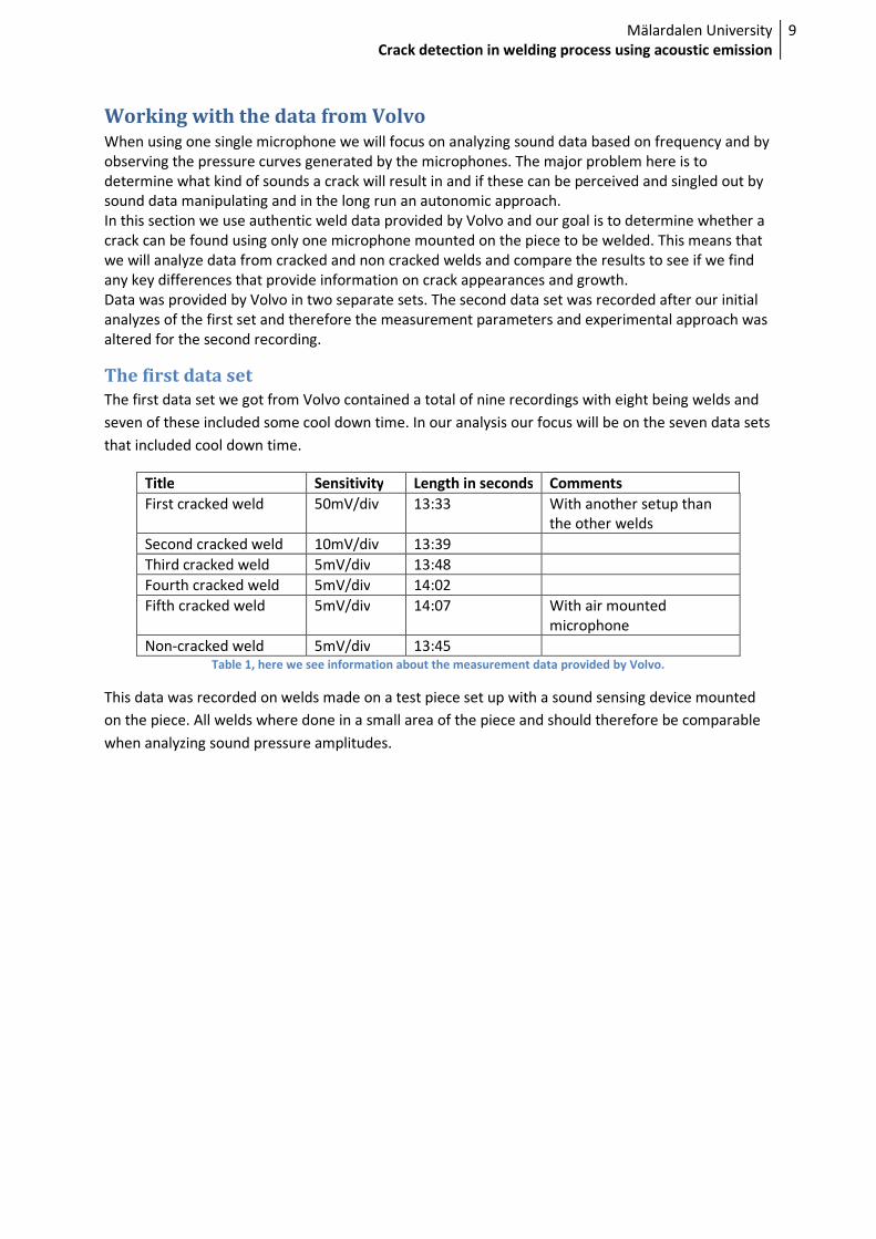
The first data set
The first data set we got from Volvo contained a total of nine recordings with eight being welds and
seven of these included some cool down time. In our analysis our focus will be on the seven data sets
that included cool down time.
Title Sensitivity Length in seconds Comments
First cracked weld 50mV/div 13:33 With another setup than
the other welds
Second cracked weld 10mV/div 13:39
Third cracked weld 5mV/div 13:48
Fourth cracked weld 5mV/div 14:02
Fifth cracked weld 5mV/div 14:07 With air mounted
microphone
Non-cracked weld 5mV/div 13:45 Table 1, here we see information about the measurement data provided by Volvo.
This data was recorded on welds made on a test piece set up with a sound sensing device mounted
on the piece. All welds where done in a small area of the piece and should therefore be comparable
when analyzing sound pressure amplitudes.

Mälardalen University
Crack detection in welding process using acoustic emission
10
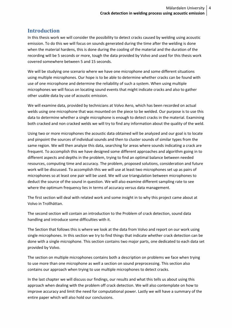
Figure 1, the setup used by the people at Volvo to record data set 1.
In figure 1 we see the setup that was used at Volvo to make the recordings. At the point marked A in
the top left half of the figure we see the microphone mounted on the piece. At point B in the right
part of the figure is where the welding took place. All welds where made in the polished area and
where made from top to bottom given the perspective of the figure.
Mälardalen University
Crack detection in welding process using acoustic emission
11
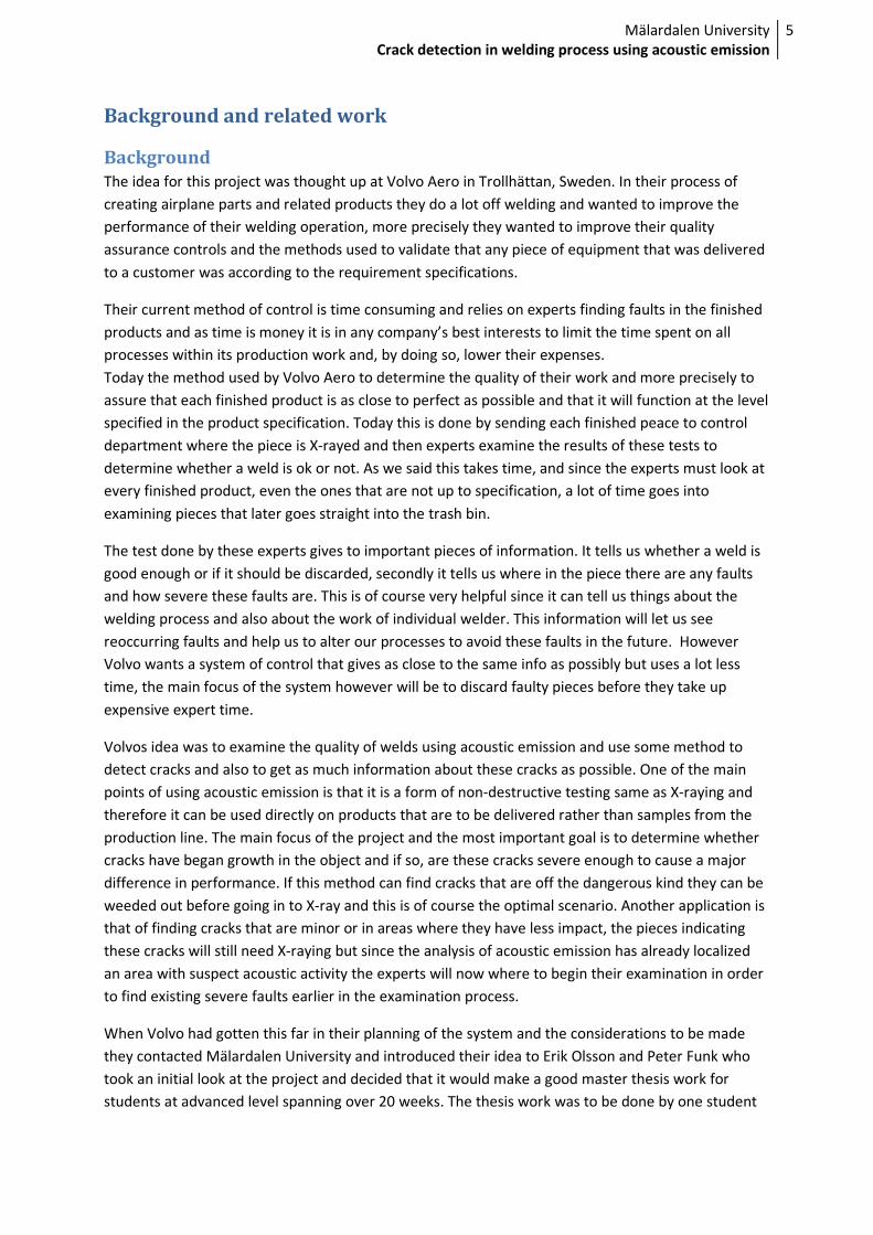
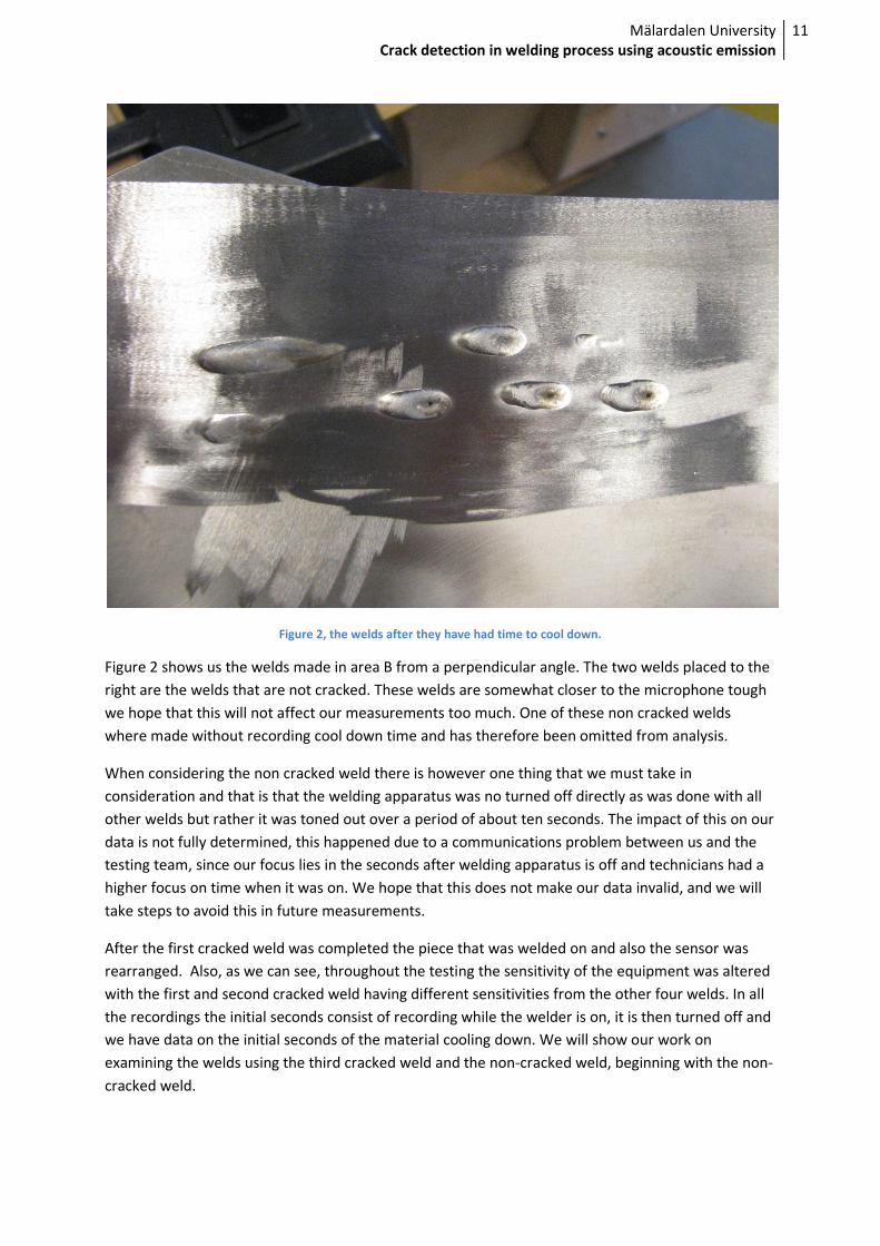
Figure 2, the welds after they have had time to cool down.
Figure 2 shows us the welds made in area B from a perpendicular angle. The two welds placed to the
right are the welds that are not cracked. These welds are somewhat closer to the microphone tough
we hope that this will not affect our measurements too much. One of these non cracked welds
where made without recording cool down time and has therefore been omitted from analysis.
When considering the non cracked weld there is however one thing that we must take in
consideration and that is that the welding apparatus was no turned off directly as was done with all
other welds but rather it was toned out over a period of about ten seconds. The impact of this on our
data is not fully determined, this happened due to a communications problem between us and the
testing team, since our focus lies in the seconds after welding apparatus is off and technicians had a
higher focus on time when it was on. We hope that this does not make our data invalid, and we will
take steps to avoid this in future measurements.
After the first cracked weld was completed the piece that was welded on and also the sensor was
rearranged. Also, as we can see, throughout the testing the sensitivity of the equipment was altered
with the first and second cracked weld having different sensitivities from the other four welds. In all
the recordings the initial seconds consist of recording while the welder is on, it is then turned off and
we have data on the initial seconds of the material cooling down. We will show our work on
examining the welds using the third cracked weld and the non-cracked weld, beginning with the non-
cracked weld.

Mälardalen University
Crack detection in welding process using acoustic emission
12
Examining the non-cracked weld
The first step we took when examining the sound data was naturally to look at a plot of the sound
pressure over time.
Figure 3, the non cracked weld shown as sound pressure over time.
Above in figure 3 we see the data plot and we can notice the change around index 7 on the X-axis,
this is where the welding apparatus was turned off. Since we will want to take closer look on the part
of the data that was gathered after the weld was turned off we cut that data out and worked on it
exclusively. This leaves us with a new array consisting of indexes 7000000 to 10000000 of the original
data array.
Figure 4, the last part of our sound data, recorded with welding apparatus off.
Mälardalen University
Crack detection in welding process using acoustic emission
13
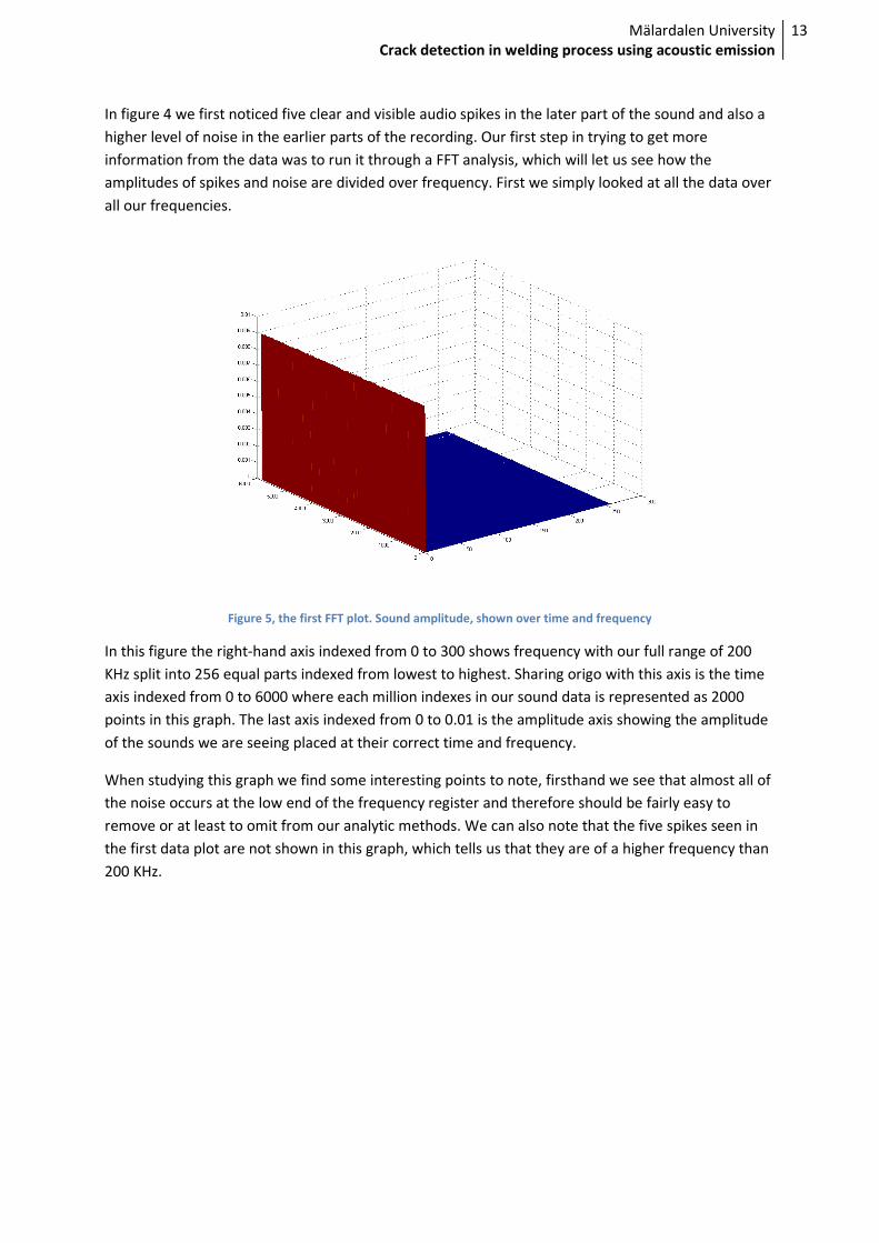
In figure 4 we first noticed five clear and visible audio spikes in the later part of the sound and also a
higher level of noise in the earlier parts of the recording. Our first step in trying to get more
information from the data was to run it through a FFT analysis, which will let us see how the
amplitudes of spikes and noise are divided over frequency. First we simply looked at all the data over
all our frequencies.
Figure 5, the first FFT plot. Sound amplitude, shown over time and frequency
In this figure the right-hand axis indexed from 0 to 300 shows frequency with our full range of 200
KHz split into 256 equal parts indexed from lowest to highest. Sharing origo with this axis is the time
axis indexed from 0 to 6000 where each million indexes in our sound data is represented as 2000
points in this graph. The last axis indexed from 0 to 0.01 is the amplitude axis showing the amplitude
of the sounds we are seeing placed at their correct time and frequency.
When studying this graph we find some interesting points to note, firsthand we see that almost all of
the noise occurs at the low end of the frequency register and therefore should be fairly easy to
remove or at least to omit from our analytic methods. We can also note that the five spikes seen in
the first data plot are not shown in this graph, which tells us that they are of a higher frequency than
200 KHz.
Mälardalen University
Crack detection in welding process using acoustic emission
14
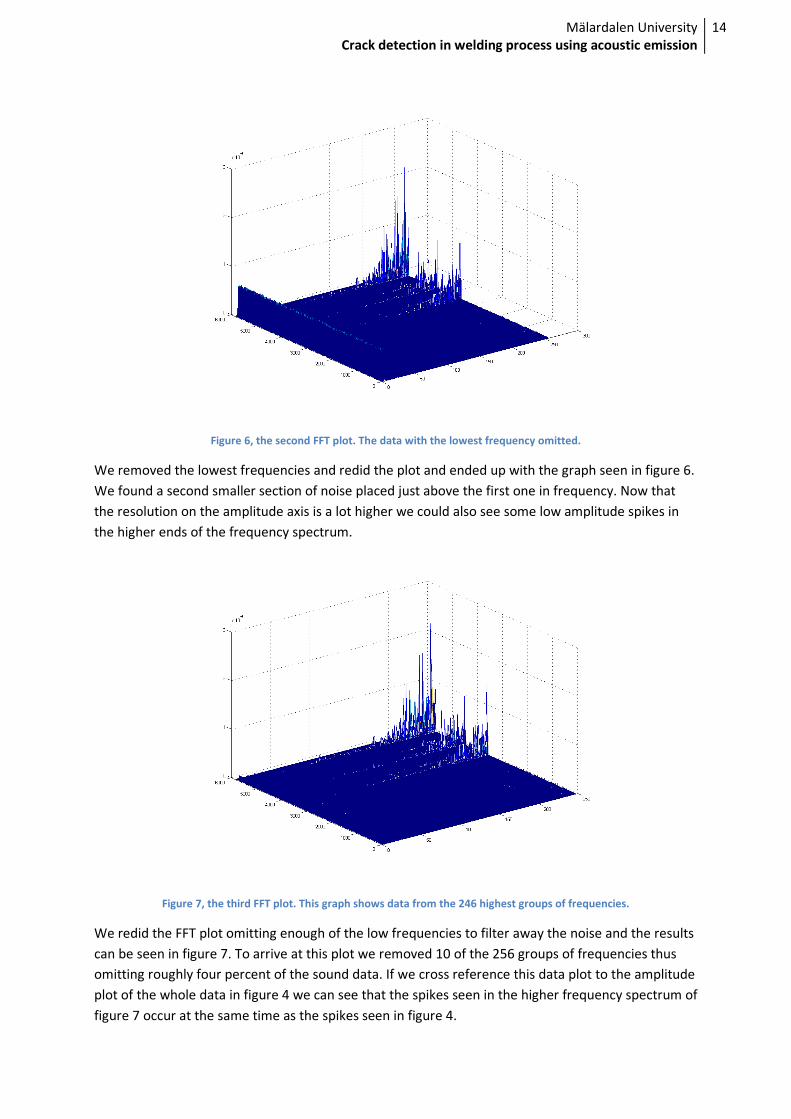
Figure 6, the second FFT plot. The data with the lowest frequency omitted.
We removed the lowest frequencies and redid the plot and ended up with the graph seen in figure 6.
We found a second smaller section of noise placed just above the first one in frequency. Now that
the resolution on the amplitude axis is a lot higher we could also see some low amplitude spikes in
the higher ends of the frequency spectrum.
Figure 7, the third FFT plot. This graph shows data from the 246 highest groups of frequencies.
We redid the FFT plot omitting enough of the low frequencies to filter away the noise and the results
can be seen in figure 7. To arrive at this plot we removed 10 of the 256 groups of frequencies thus
omitting roughly four percent of the sound data. If we cross reference this data plot to the amplitude
plot of the whole data in figure 4 we can see that the spikes seen in the higher frequency spectrum of
figure 7 occur at the same time as the spikes seen in figure 4.
Mälardalen University
Crack detection in welding process using acoustic emission
15
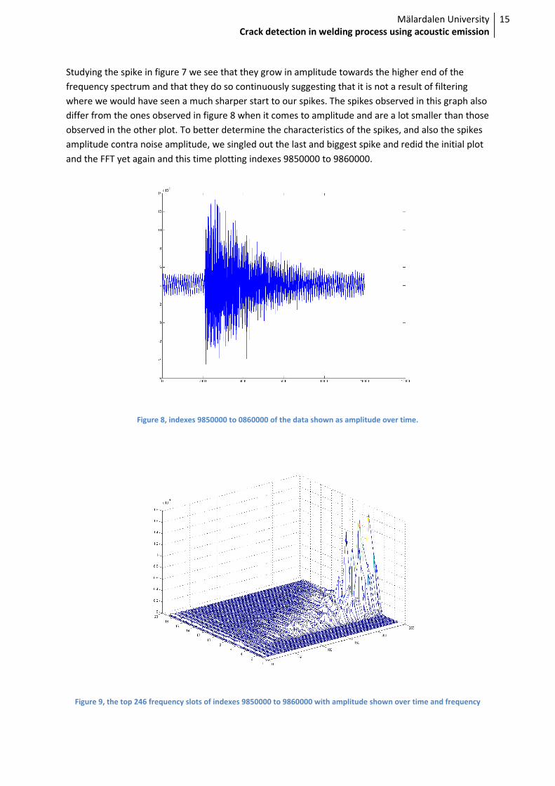
Studying the spike in figure 7 we see that they grow in amplitude towards the higher end of the
frequency spectrum and that they do so continuously suggesting that it is not a result of filtering
where we would have seen a much sharper start to our spikes. The spikes observed in this graph also
differ from the ones observed in figure 8 when it comes to amplitude and are a lot smaller than those
observed in the other plot. To better determine the characteristics of the spikes, and also the spikes
amplitude contra noise amplitude, we singled out the last and biggest spike and redid the initial plot
and the FFT yet again and this time plotting indexes 9850000 to 9860000.
Figure 8, indexes 9850000 to 0860000 of the data shown as amplitude over time.
Figure 9, the top 246 frequency slots of indexes 9850000 to 9860000 with amplitude shown over time and frequency
Mälardalen University
Crack detection in welding process using acoustic emission
16
In figures 8 and 9 we see a smaller portion of the data represented in three different ways. First in
figure 8 we see the data one again as sound pressure amplitude over time, in this graph we can see
the spikes from figure 8 but this time the resolution of the axis has changed and we also see that the
start of the spike is really fast whilst it ends by fading out.
Studying figure 9 we see the spike and how it is fading out and how that spreads over the frequency
slots. We that the highest amplitude in the spike is found at the high end of the observed frequency
slots, this leads us to assume that an even higher peak can be found at higher frequencies. Since we
still cannot see peaks to match those of figure 4 we will have to keep searching or do other
measurements.
In the close up in figure 9 we can also see some effects from the noise climbing its way up in
frequency. The affect is fading and it is fixed in frequency which will make it easier to suppress if that
turns out to be necessary.
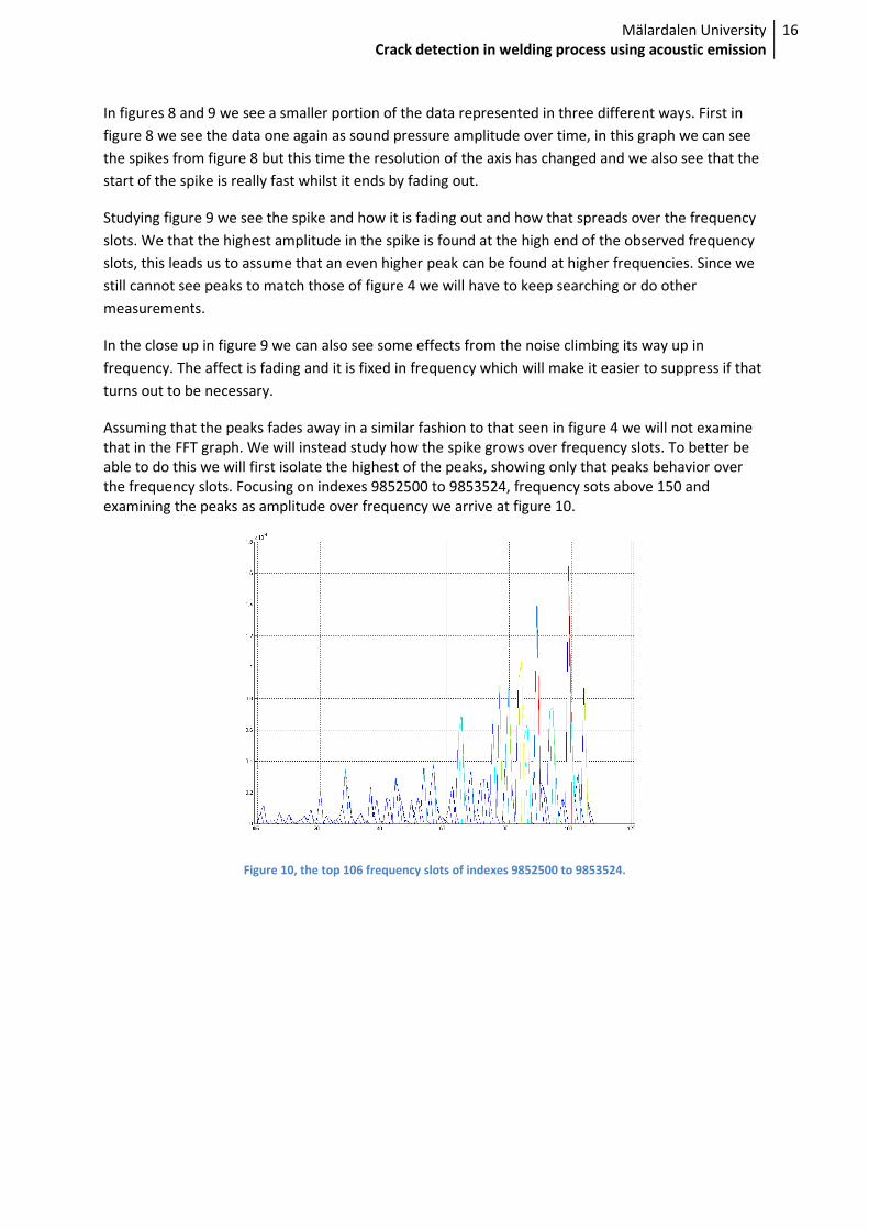
Assuming that the peaks fades away in a similar fashion to that seen in figure 4 we will not examine
that in the FFT graph. We will instead study how the spike grows over frequency slots. To better be
able to do this we will first isolate the highest of the peaks, showing only that peaks behavior over
the frequency slots. Focusing on indexes 9852500 to 9853524, frequency sots above 150 and
examining the peaks as amplitude over frequency we arrive at figure 10.
Figure 10, the top 106 frequency slots of indexes 9852500 to 9853524.
Mälardalen University
Crack detection in welding process using acoustic emission
17
From the way the observed amplitudes in figure 10 behave we assume that the biggest amplitude
can be found at higher frequencies. This leads us to speculate whether the amplitude spikes seen in
figure 4 are located at an even higher frequency than the ones covered by our measurements. From
the figure we also see that the relationship between frequency and amplitude is varying and it seems
that there are peaks at higher and higher frequencies but also smaller peaks at frequencies in
between. From the figure it is not possible to approximate a frequency at which we will find our
sought after amplitude peaks. We do believe however since we see amplitudes of varying height over
the frequencies, but still all growing with the frequency that, there might be waves carried by each
other. To determine if this is the case we made a high-resolution close up of the peak as amplitude
over time, similar to figure 4.
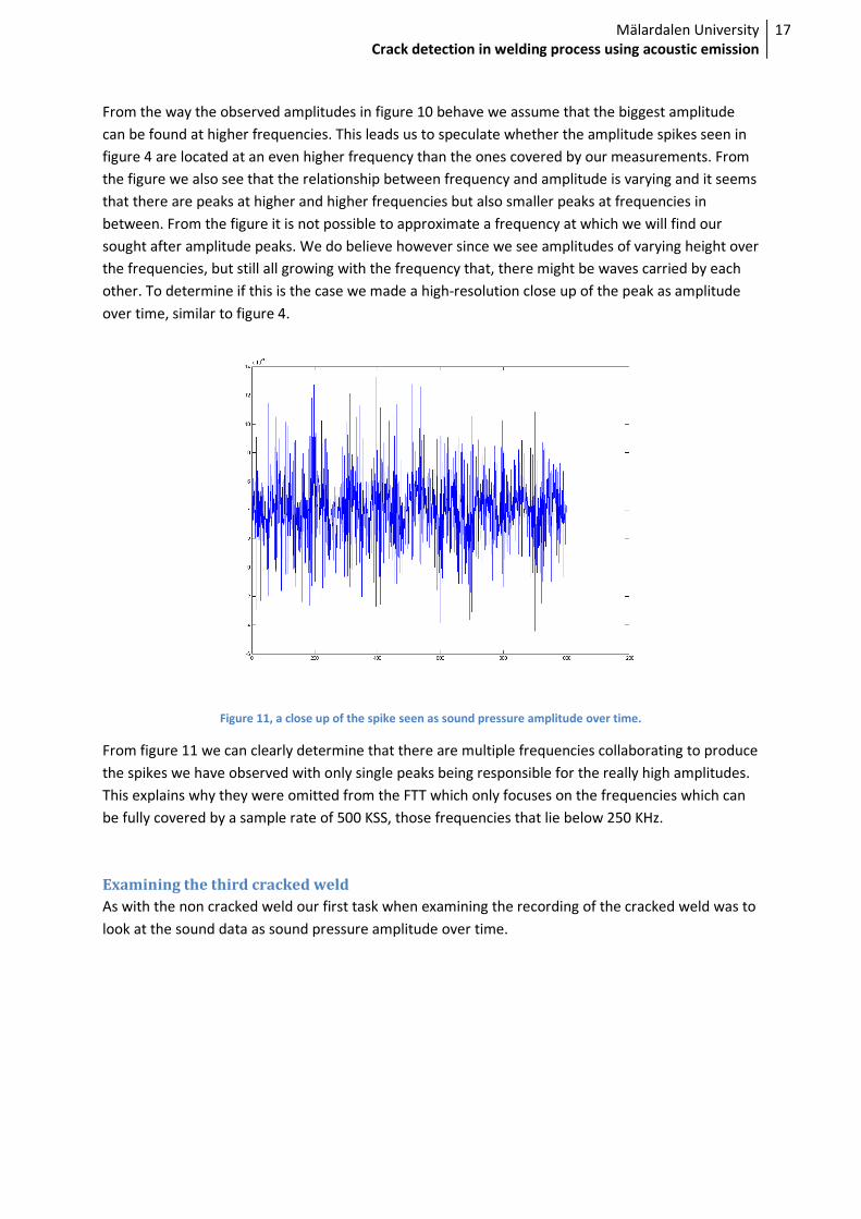
Figure 11, a close up of the spike seen as sound pressure amplitude over time.
From figure 11 we can clearly determine that there are multiple frequencies collaborating to produce
the spikes we have observed with only single peaks being responsible for the really high amplitudes.
This explains why they were omitted from the FTT which only focuses on the frequencies which can
be fully covered by a sample rate of 500 KSS, those frequencies that lie below 250 KHz.
Examining the third cracked weld
As with the non cracked weld our first task when examining the recording of the cracked weld was to
look at the sound data as sound pressure amplitude over time.
Mälardalen University
Crack detection in welding process using acoustic emission
18
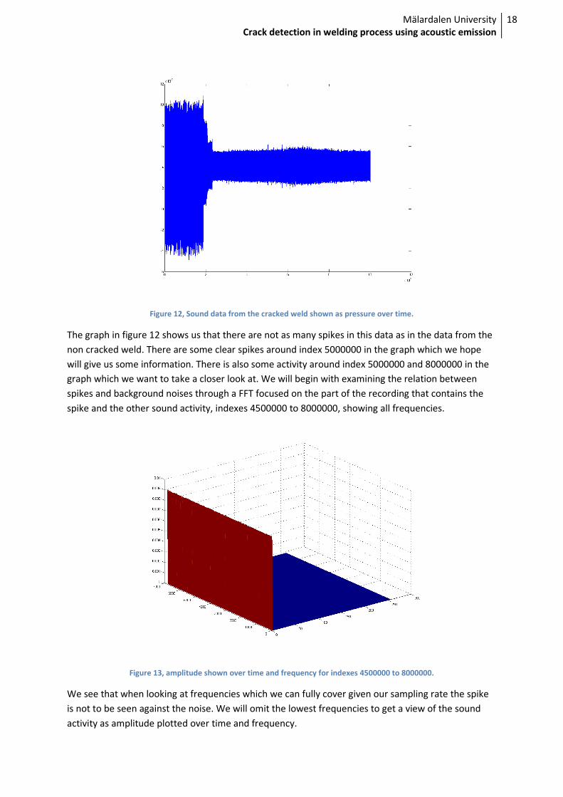
Figure 12, Sound data from the cracked weld shown as pressure over time.
The graph in figure 12 shows us that there are not as many spikes in this data as in the data from the
non cracked weld. There are some clear spikes around index 5000000 in the graph which we hope
will give us some information. There is also some activity around index 5000000 and 8000000 in the
graph which we want to take a closer look at. We will begin with examining the relation between
spikes and background noises through a FFT focused on the part of the recording that contains the
spike and the other sound activity, indexes 4500000 to 8000000, showing all frequencies.
Figure 13, amplitude shown over time and frequency for indexes 4500000 to 8000000.
We see that when looking at frequencies which we can fully cover given our sampling rate the spike
is not to be seen against the noise. We will omit the lowest frequencies to get a view of the sound
activity as amplitude plotted over time and frequency.
Mälardalen University
Crack detection in welding process using acoustic emission
19
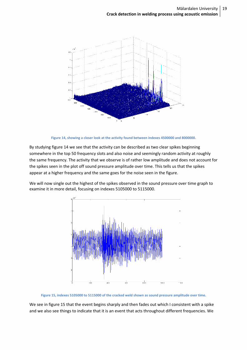
Figure 14, showing a closer look at the activity found between indexes 4500000 and 8000000.
By studying figure 14 we see that the activity can be described as two clear spikes beginning
somewhere in the top 50 frequency slots and also noise and seemingly random activity at roughly
the same frequency. The activity that we observe is of rather low amplitude and does not account for
the spikes seen in the plot off sound pressure amplitude over time. This tells us that the spikes
appear at a higher frequency and the same goes for the noise seen in the figure.
We will now single out the highest of the spikes observed in the sound pressure over time graph to
examine it in more detail, focusing on indexes 5105000 to 5115000.
Figure 15, indexes 5105000 to 5115000 of the cracked weld shown as sound pressure amplitude over time.
We see in figure 15 that the event begins sharply and then fades out which I consistent with a spike
and we also see things to indicate that it is an event that acts throughout different frequencies. We
Mälardalen University
Crack detection in welding process using acoustic emission
20
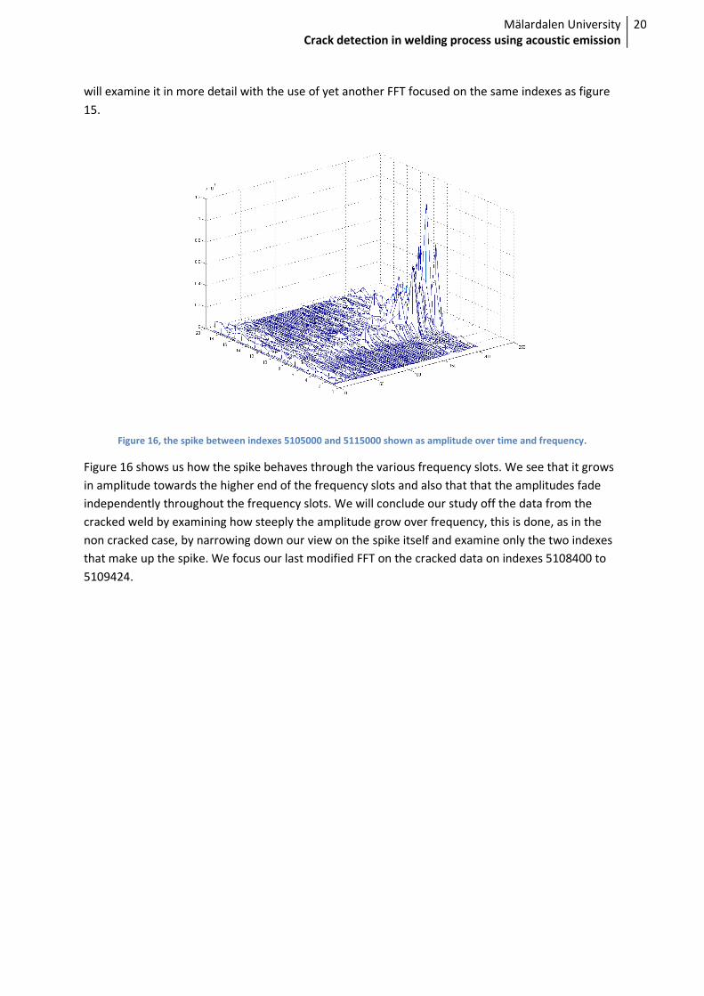
will examine it in more detail with the use of yet another FFT focused on the same indexes as figure
15.
Figure 16, the spike between indexes 5105000 and 5115000 shown as amplitude over time and frequency.
Figure 16 shows us how the spike behaves through the various frequency slots. We see that it grows
in amplitude towards the higher end of the frequency slots and also that that the amplitudes fade
independently throughout the frequency slots. We will conclude our study off the data from the
cracked weld by examining how steeply the amplitude grow over frequency, this is done, as in the
non cracked case, by narrowing down our view on the spike itself and examine only the two indexes
that make up the spike. We focus our last modified FFT on the cracked data on indexes 5108400 to
5109424.
Mälardalen University
Crack detection in welding process using acoustic emission
21
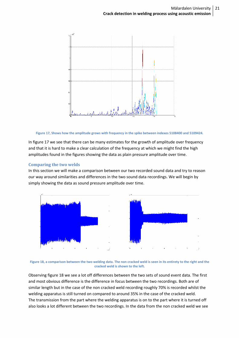
Figure 17, Shows how the amplitude grows with frequency in the spike between indexes 5108400 and 5109424.
In figure 17 we see that there can be many estimates for the growth of amplitude over frequency
and that it is hard to make a clear calculation of the frequency at which we might find the high
amplitudes found in the figures showing the data as plain pressure amplitude over time.
Comparing the two welds
In this section we will make a comparison between our two recorded sound data and try to reason
our way around similarities and differences in the two sound data recordings. We will begin by
simply showing the data as sound pressure amplitude over time.
Figure 18, a comparison between the two welding data. The non cracked weld is seen in its entirety to the right and the
cracked weld is shown to the left.
Observing figure 18 we see a lot off differences between the two sets of sound event data. The first
and most obvious difference is the difference in focus between the two recordings. Both are of
similar length but in the case of the non cracked weld recording roughly 70% is recorded whilst the
welding apparatus is still turned on compared to around 35% in the case of the cracked weld.
The transmission from the part where the welding apparatus is on to the part where it is turned off
also looks a lot different between the two recordings. In the data from the non cracked weld we see
Mälardalen University
Crack detection in welding process using acoustic emission
22
what looks like an immediate turning of off the apparatus, the transition from on to off is done in one
single step and in a very small timeframe. Whereas in the case of the cracked weld the apparatus is
turned off successively through several steps and also the turning of takes up more time than in the
recording from the non cracked weld. It is not clear if and how this affects our data but the issue has
been noted and will be taken into account when conducting the recordings for our second data set.
Another thing that we can see clearly from the figure is the difference in behaviors of the spikes
between the two recordings. There are clear spikes in both cases but there are big differences
between them both in number, frequency and amplitude. (Notice that frequency in this sense
corresponds to the number of spikes and their relative timing rather than the frequency of the
sounds that generate the spikes). In the recording from the non cracked weld we see a number of
high to medium amplitude spikes with short time in between beginning roughly two seconds after
the apparatus is turned off. In the recording from the cracked weld we see one medium amplitude
spike and some small spikes spaced out throughout the recording with the highest spike at about 3
seconds after the apparatus is turned off.
In both recordings we see some noises that differ from the base level of noise though it appears at
different timing in the recordings and also varies in length between them.
These differences are consistent throughout all the data with all recordings from cracked welds
showing medium to low amplitude spikes and not as many occurrences as in the case of the non
cracked weld.
Note worthy similarities between our recordings on this stage is that the sound pressure amplitude
recorded whilst the apparatus is on and also the noise when it has been turned off is at close to the
same level and also that it acts the same which tells us that the experiments have been conducted
with roughly the same environmental parameters.
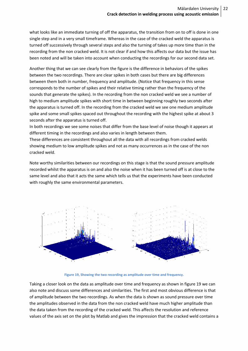
Figure 19, Showing the two recording as amplitude over time and frequency.
Taking a closer look on the data as amplitude over time and frequency as shown in figure 19 we can
also note and discuss some differences and similarities. The first and most obvious difference is that
of amplitude between the two recordings. As when the data is shown as sound pressure over time
the amplitudes observed in the data from the non cracked weld have much higher amplitude than
the data taken from the recording of the cracked weld. This affects the resolution and reference
values of the axis set on the plot by Matlab and gives the impression that the cracked weld contains a

Mälardalen University
Crack detection in welding process using acoustic emission
23
lot more noise spread out over the frequencies. This however in not true it is merely the higher
resolution in the graph showing that data that gives the illusion of a higher noise.
We note that the noise seen in the pressure over time graphs described as deviating from the
background noises can be observed at the high end of the frequency slot in both graphs and is visible
in the non cracked weld data even though the resolution is lower than in the cracked weld data. This
noise is seen prior to the spikes in the data from the non cracked weld and directly after the spikes in
the data recorded on the cracked weld.
Furthermore we can also see that the spikes, apart from the difference in amplitude, are similar in
both data sets. Particularly their growth and the behavior of their respective amplitude as the
frequency increases are very similar. We will take a closer look at the spikes to conclude our
comparison of the two data sets.
Figure 20, a close up FFT made on the largest spikes from both data sets, the one from the non cracked weld is shown to
the left and the data from the cracked weld is to the right.
Examining the two graphs in figure 20 we see a lot of similarities between the two spikes. We see
that their behavior regarding both time and frequency is very much alike and this gives strength to
our theories that claim that the events in themselves are similar. The only significant difference is yet
again the amplitude and a small variation to the fading out of the sound pressure at high frequencies,
though this can be explained by the difference in resolution.
Conclusion
We conclude that, as far as we can see in this data, the same type off sound generating events occur
in both cracked and non cracked welds and that we will have to achieve measurements that give us a
larger number of spikes to work with from both kinds of welds, preferably the new data will have the
same consistency in amplitude as we have so far observed in behavior.
We will also want new data with a higher sampling rate so that we can observe the whole sound
events. Preferably we want to include frequencies where the spikes are no longer active so that we
can watch their behaviors over all the frequencies that they inhabit.
So far we see no difference between cracked and non cracked welds and we lean towards the idea
that we need to categorize number of sound events and use some sort of localization techniques to
determine whether cracks are present or not, work on the second data set will help to confirm or
deny this hypothesis.

Mälardalen University
Crack detection in welding process using acoustic emission
24
The Second Data Set
The second data set we received from Volvo contained a total of six recordings and five of these
where recorded during welding. A similar equipment setup as for the first data set was used apart
from the recording in itself which was done with other parameters.
For this data set they used a sample rate of two million samples per second which is four times the
sampling rate used for the first dataset. All recordings where done with the same microphone
sensitivity and again at roughly the same distance. The sensitivity was set to 20 mV per div.
One of the welds in the set was made with a long shutdown time for the welding apparatus and all
the other used a short shutdown time. Some differences occurs even among the welds said to have
the same shutdown sequence and this is yet to be explained by Volvo, since this occurs at the
beginning of the recording we have not given it to much weight with our focus still lying on the later
part of the recording.
Title Sensitivity Length in seconds Comments
Non cracked weld 20mV/div 13:29 Longer turning off of
welding apparatus
First cracked weld 20mV/div 13:33
No visible cracks 20mV/div 13:36
Second cracked weld 20mV/div 14:41
Third cracked weld 20mV/div 14:44
Fourth cracked weld 20mV/div 13:48 Table 2, this table shows the welds from data set 2.
At first glance we cannot see any clear spikes in the data from the two welds without visible cracks
but still see clear spikes in the cracked welds. Since all the cracked welds are very similar to one
another we will use one of these to represent them all and we will also examine the non cracked
weld and the weld without visible cracks, beginning with the non cracked weld. For all welds we
divided the plotting of the data into two parts, one showing the time when the welding apparatus
was on and the turning of off the apparatus, the other parts shows the interesting data gathered
from the initial cooling of the material.
Non cracked weld
We began by examining the data that was recorded during the non cracked weld. This weld was done
with a longer tone out of the welding apparatus. We plotted the data in two parts with the first
containing the turning of off the apparatus and the other focusing on the interesting part where the
material starts to cool down. The two parts of the data is shown with different values for the Y-axis
to get a better understanding of both the noise produced by the welding apparatus and the sound
data recorded during cooling.
Mälardalen University
Crack detection in welding process using acoustic emission
25
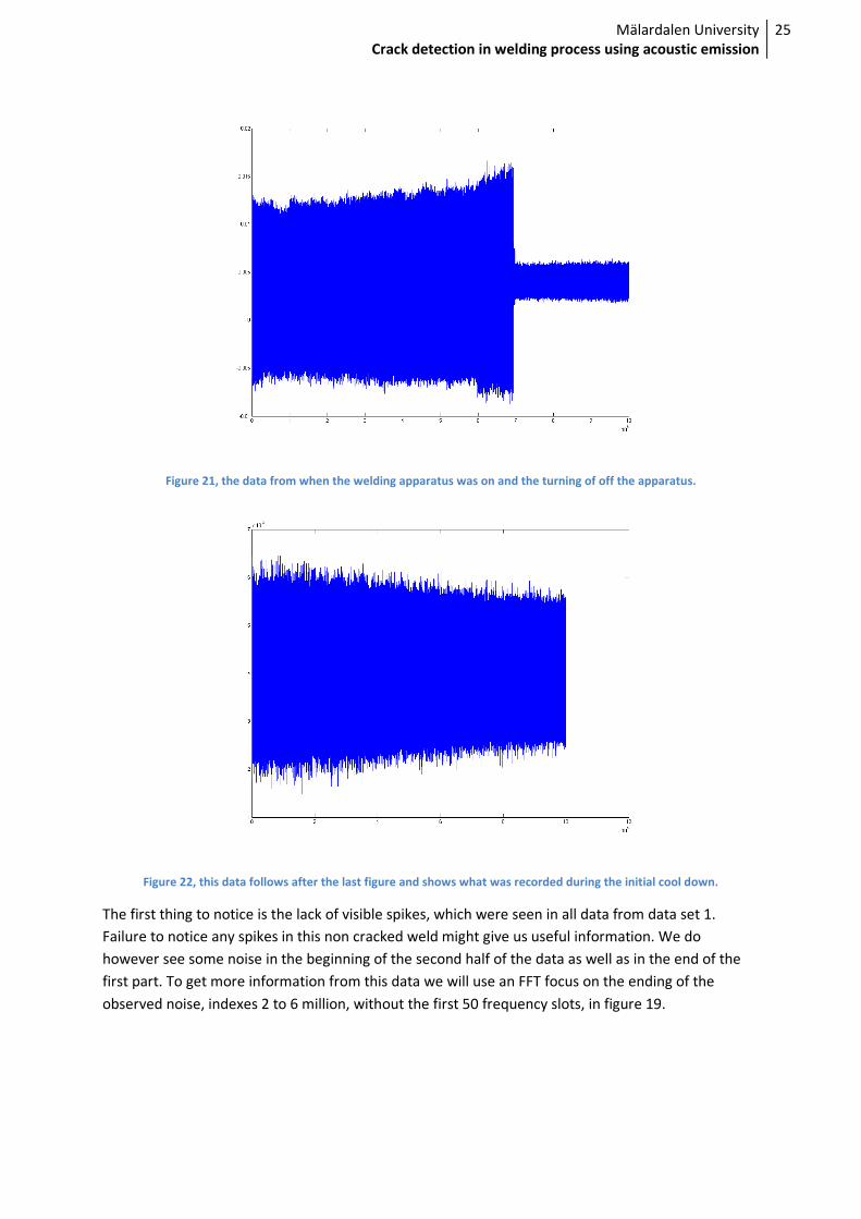
Figure 21, the data from when the welding apparatus was on and the turning of off the apparatus.
Figure 22, this data follows after the last figure and shows what was recorded during the initial cool down.
The first thing to notice is the lack of visible spikes, which were seen in all data from data set 1.
Failure to notice any spikes in this non cracked weld might give us useful information. We do
however see some noise in the beginning of the second half of the data as well as in the end of the
first part. To get more information from this data we will use an FFT focus on the ending of the
observed noise, indexes 2 to 6 million, without the first 50 frequency slots, in figure 19.
Mälardalen University
Crack detection in welding process using acoustic emission
26
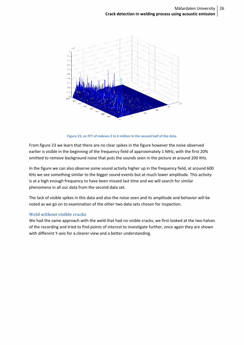
Figure 23, an FFT of indexes 2 to 6 million in the second half of the data.
From figure 23 we learn that there are no clear spikes in the figure however the noise observed
earlier is visible in the beginning of the frequency field of approximately 1 MHz, with the first 20%
omitted to remove background noise that puts the sounds seen in the picture at around 200 KHz.
In the figure we can also observe some sound activity higher up in the frequency field, at around 600
KHz we see something similar to the bigger sound events but at much lower amplitude. This activity
is at a high enough frequency to have been missed last time and we will search for similar
phenomena in all our data from the second data set.
The lack of visible spikes in this data and also the noise seen and its amplitude and behavior will be
noted as we go on to examination of the other two data sets chosen for inspection.
Weld without visible cracks
We had the same approach with the weld that had no visible cracks; we first looked at the two halves
of the recording and tried to find points of interest to investigate further, once again they are shown
with different Y-axis for a clearer view and a better understanding.
Mälardalen University
Crack detection in welding process using acoustic emission
27
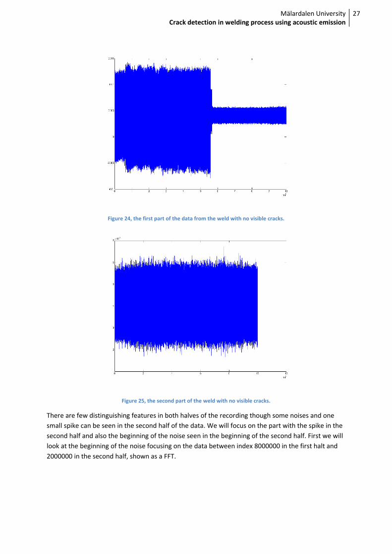
Figure 24, the first part of the data from the weld with no visible cracks.
Figure 25, the second part of the weld with no visible cracks.
There are few distinguishing features in both halves of the recording though some noises and one
small spike can be seen in the second half of the data. We will focus on the part with the spike in the
second half and also the beginning of the noise seen in the beginning of the second half. First we will
look at the beginning of the noise focusing on the data between index 8000000 in the first halt and
2000000 in the second half, shown as a FFT.
Mälardalen University
Crack detection in welding process using acoustic emission
28
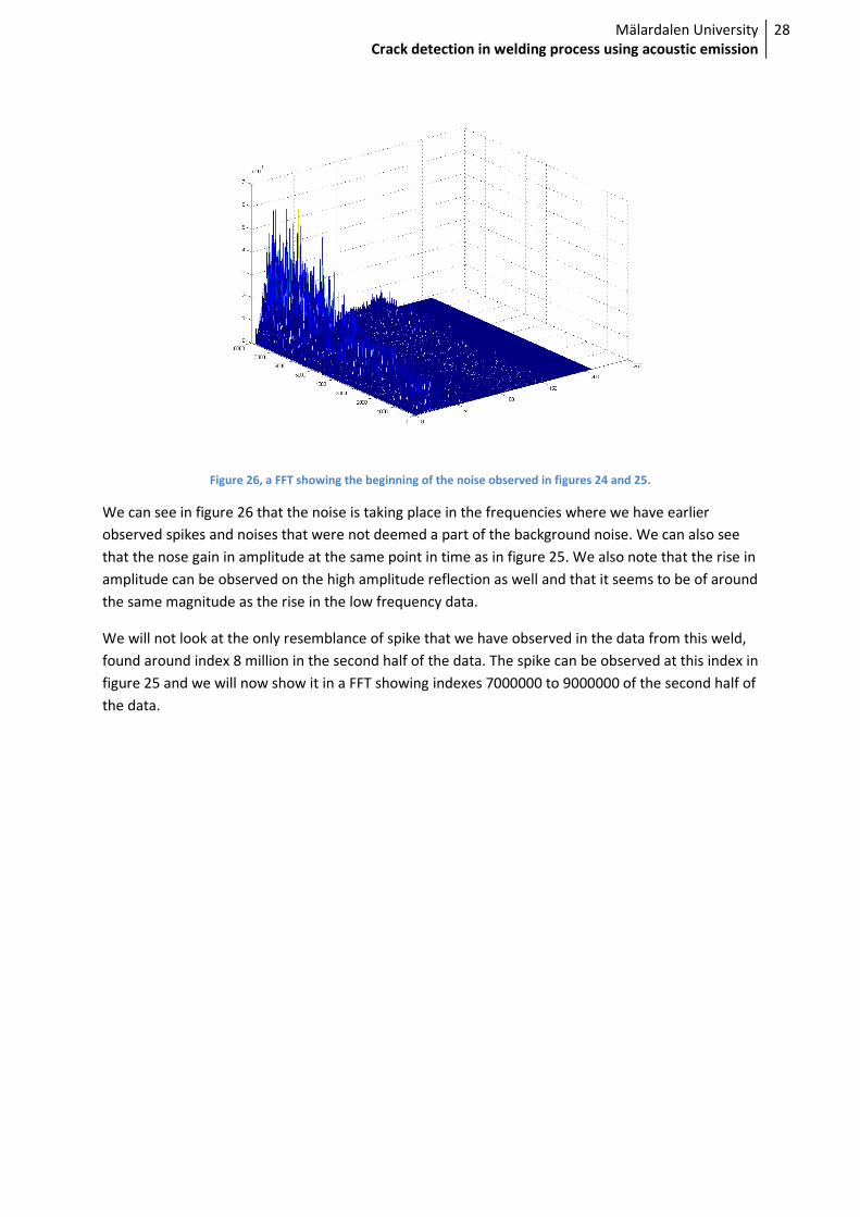
Figure 26, a FFT showing the beginning of the noise observed in figures 24 and 25.
We can see in figure 26 that the noise is taking place in the frequencies where we have earlier
observed spikes and noises that were not deemed a part of the background noise. We can also see
that the nose gain in amplitude at the same point in time as in figure 25. We also note that the rise in
amplitude can be observed on the high amplitude reflection as well and that it seems to be of around
the same magnitude as the rise in the low frequency data.
We will not look at the only resemblance of spike that we have observed in the data from this weld,
found around index 8 million in the second half of the data. The spike can be observed at this index in
figure 25 and we will now show it in a FFT showing indexes 7000000 to 9000000 of the second half of
the data.
Mälardalen University
Crack detection in welding process using acoustic emission
29
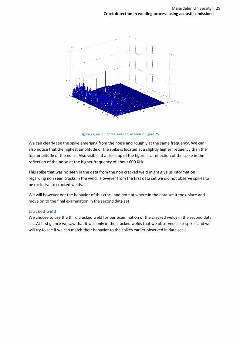
Figure 27, an FFT of the small spike seen in figure 25.
We can clearly see the spike emerging from the noise and roughly at the same frequency. We can
also notice that the highest amplitude of the spike is located at a slightly higher frequency than the
top amplitude of the noise. Also visible at a close up of the figure is a reflection of the spike in the
reflection of the noise at the higher frequency of about 600 KHz.
This spike that was no seen in the data from the non cracked weld might give us information
regarding non seen cracks in the weld. However from the first data set we did not observe spikes to
be exclusive to cracked welds.
We will however not the behavior of this crack and note at where in the data set it took place and
move on to the final examination in the second data set.
Cracked weld
We choose to use the third cracked weld for our examination of the cracked welds in the second data
set. At first glance we saw that it was only in the cracked welds that we observed clear spikes and we
will try to see if we can match their behavior to the spikes earlier observed in data set 1.
Mälardalen University
Crack detection in welding process using acoustic emission
30
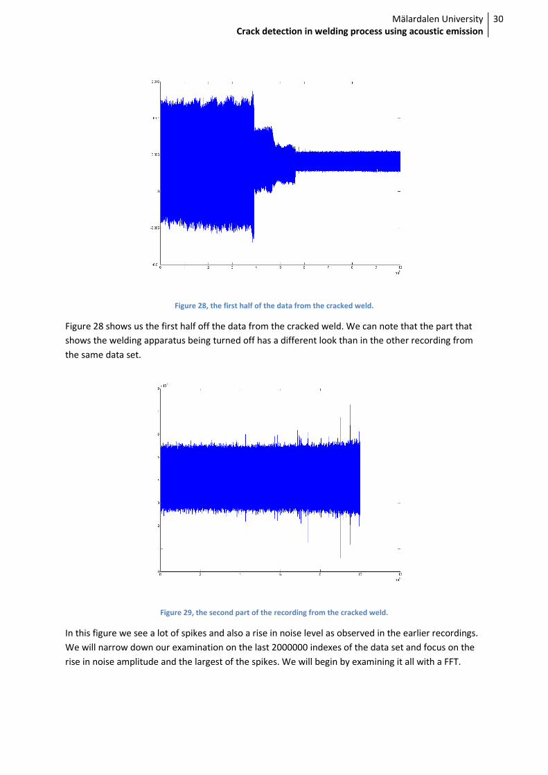
Figure 28, the first half of the data from the cracked weld.
Figure 28 shows us the first half off the data from the cracked weld. We can note that the part that
shows the welding apparatus being turned off has a different look than in the other recording from
the same data set.
Figure 29, the second part of the recording from the cracked weld.
In this figure we see a lot of spikes and also a rise in noise level as observed in the earlier recordings.
We will narrow down our examination on the last 2000000 indexes of the data set and focus on the
rise in noise amplitude and the largest of the spikes. We will begin by examining it all with a FFT.
Mälardalen University
Crack detection in welding process using acoustic emission
31
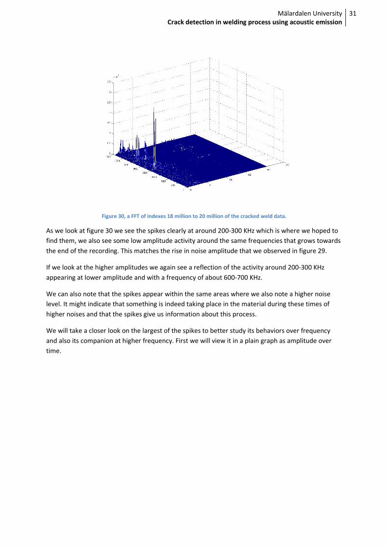
Figure 30, a FFT of indexes 18 million to 20 million of the cracked weld data.
As we look at figure 30 we see the spikes clearly at around 200-300 KHz which is where we hoped to
find them, we also see some low amplitude activity around the same frequencies that grows towards
the end of the recording. This matches the rise in noise amplitude that we observed in figure 29.
If we look at the higher amplitudes we again see a reflection of the activity around 200-300 KHz
appearing at lower amplitude and with a frequency of about 600-700 KHz.
We can also note that the spikes appear within the same areas where we also note a higher noise
level. It might indicate that something is indeed taking place in the material during these times of
higher noises and that the spikes give us information about this process.
We will take a closer look on the largest of the spikes to better study its behaviors over frequency
and also its companion at higher frequency. First we will view it in a plain graph as amplitude over
time.

Mälardalen University
Crack detection in welding process using acoustic emission
32
Figure 31, the largest spike from the cracked weld shown as amplitude over time.
When we examine the spike more closely as in figure 31 we see that I fades out in stages, the fist
max point stands alone but after it comes 5 points that reach about the same height and then I fades
again to a number of points in the next category of amplitude. I we look at the lower spikes, the
minimum points we also see roughly the same behavior, though the time of their lowest point does
not match that of the top point.
Figure 32, a FFT of the largest spike in the data from the cracked weld.
Now that we can see the spike in more detail in figure 32 we can study its behavior more closely. We
see that the event peaks at around 200 KHz which means that we were close to seeing the peak in
the first data set. The over tone at 600KHZ is a reflection of the first sound and was of course omitted
Mälardalen University
Crack detection in welding process using acoustic emission
33
earlier. Now that we have identified a so clear a spike in the data and also noted that it lies within a
period of higher noises we are starting to assume that a correlation between spikes and a rise in the
noise level, only measuring noise around 100-200 KHz might actually indicate an event taking place in
the material.
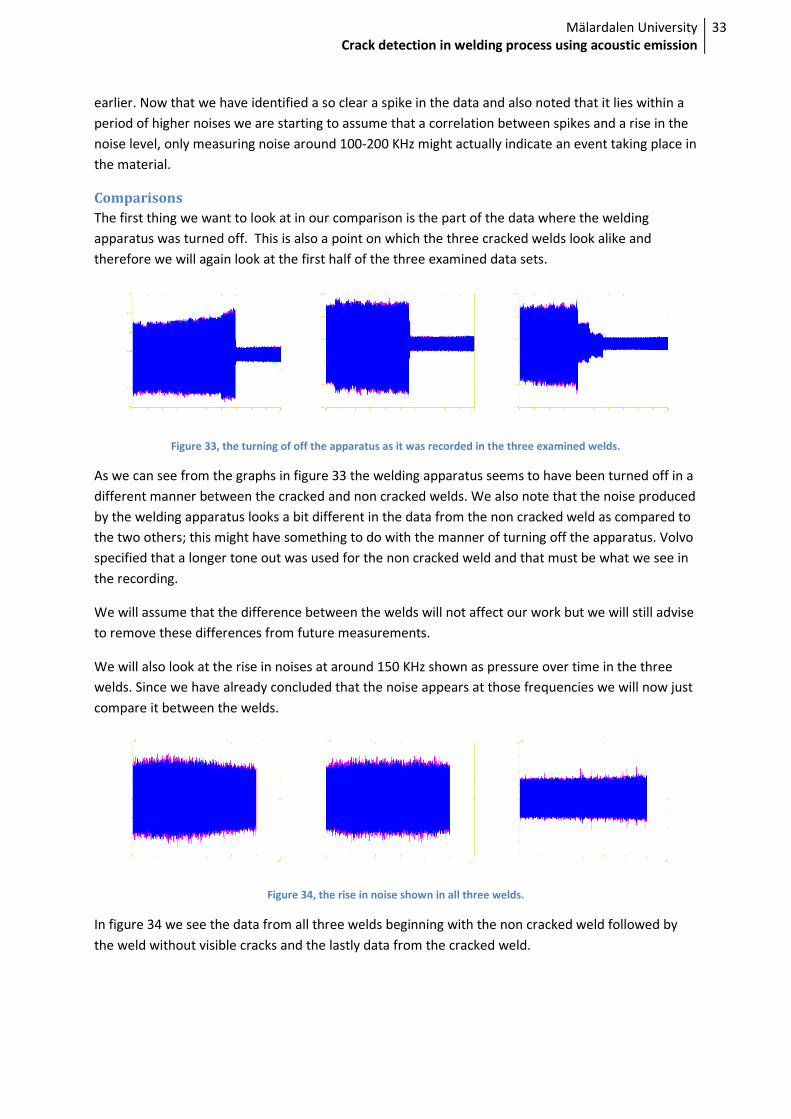
Comparisons
The first thing we want to look at in our comparison is the part of the data where the welding
apparatus was turned off. This is also a point on which the three cracked welds look alike and
therefore we will again look at the first half of the three examined data sets.
Figure 33, the turning of off the apparatus as it was recorded in the three examined welds.
As we can see from the graphs in figure 33 the welding apparatus seems to have been turned off in a
different manner between the cracked and non cracked welds. We also note that the noise produced
by the welding apparatus looks a bit different in the data from the non cracked weld as compared to
the two others; this might have something to do with the manner of turning off the apparatus. Volvo
specified that a longer tone out was used for the non cracked weld and that must be what we see in
the recording.
We will assume that the difference between the welds will not affect our work but we will still advise
to remove these differences from future measurements.
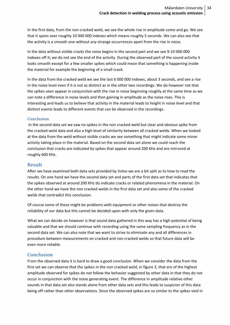
We will also look at the rise in noises at around 150 KHz shown as pressure over time in the three
welds. Since we have already concluded that the noise appears at those frequencies we will now just
compare it between the welds.
Figure 34, the rise in noise shown in all three welds.
In figure 34 we see the data from all three welds beginning with the non cracked weld followed by
the weld without visible cracks and the lastly data from the cracked weld.
Mälardalen University
Crack detection in welding process using acoustic emission
34
In the first data, from the non cracked weld, we see the whole rise in amplitude come and go. We see
that it spans over roughly 10 000 000 indexes which means roughly 5 seconds. We can also see that
the activity is a smooth one without any strange occurrences apart from the rise in noise.
In the data without visible cracks the noise begins in the second part and we see 9-10 000 000
indexes off it; we do not see the end of the activity. During the observed part of the sound activity it
looks smooth except for a few smaller spikes which could mean that something is happening inside
the material for example the beginning of a small crack.
In the data from the cracked weld we see the last 6 000 000 indexes, about 3 seconds, and see a rise
in the noise level even if it is not as distinct as in the other two recordings. We do however not that
the spikes seen appear in conjunction with the rise in noise beginning roughly at the same time as we
can note a difference in noise levels and then gaining in amplitude as the noise rises. This is
interesting and leads us to believe that activity in the material leads to height in noise level and that
distinct events leads to different events that can be observed in the recordings.
Conclusion
In the second data set we saw no spikes in the non cracked weld but clear and obvious spike from
the cracked weld data and also a high level of similarity between all cracked welds. When we looked
at the data from the weld without visible cracks we see something that might indicate some minor
activity taking place in the material. Based on the second data set alone we could reach the
conclusion that cracks are indicated by spikes that appear around 200 KHz and are mirrored at
roughly 600 KHz.
Result
After we have examined both data sets provided by Volvo we are a bit split as to how to read the
results. On one hand we have the second data set and parts of the first data set that indicates that
the spikes observed at around 200 KHz do indicate cracks or related phenomena in the material. On
the other hand we have the non cracked welds in the first data set and also some of the cracked
welds that contradict this conclusion.
Of course some of these might be problems with equipment or other noises that destroy the
reliability of our data but this cannot be decided upon with only the given data.
What we can decide on however is that sound data gathered in this way has a high potential of being
valuable and that we should continue with recording using the same sampling frequency as in the
second data set. We can also note that we want to strive to eliminate any and all differences in
procedure between measurements on cracked and non cracked welds so that future data will be
even more reliable.
Conclusion
From the observed data it is hard to draw a good conclusion. When we consider the data from the
first set we can observe that the spikes in the non cracked weld, in figure 3, that are of the highest
amplitude observed for spikes do not follow the behavior suggested by other data in that they do not
occur in conjunction with the noise generating event. The difference in amplitude relative other
sounds in that data set also stands alone from other data sets and this leads to suspicion of this data
being off rather than other observations. Since the observed spikes are so similar to the spikes vied in
Mälardalen University
Crack detection in welding process using acoustic emission
35
other data this might be because other welds are cooling off in the vicinity of the non cracked weld
or just a result of the difference in equipment sensitivity.
The conclusion we reach is that we spikes that lie within the field of heightened noise with both
spikes and noise have frequencies at around 200 KHz might very well indicate crack growth in the
material. The next step in measurements will be to conduct larger scale experiments with more cases
in each one and also to keep allowing time in between welds for the material too properly cool off
and therefore avoid any eventual interference.

Mälardalen University
Crack detection in welding process using acoustic emission
36
Proposing solutions for localization and analysis
When considering solutions to our problem we have taken a lot of things into consideration and we
have looked at a lot off possible answers. We have compared many different ideas in theory and
come up with a few different approaches to go on and test in real life situations. After our own initial
tests, which will be done on mundane data with acoustic data that lies within the hearable spectrum,
we will go on to apply the real test data on the proposed solutions that produce the results we are
looking for.
In this section we will focus on our work on design solutions for the microphone array design, the
algorithms used for sound localization, sound data handling and also on our work on recognizing
cracks in the output from the first two algorithms. The work put into these three areas will be
presented in that order, first array design then source localization followed by data handling and
lastly analyzing the data to find cracks. We will begin by taking a closer look at the some of the
problems we face.
When doing this thesis work we had some problems with measurements at Volvo and therefore we
were unable to obtain data recorded with multiple microphones, we also had problems with
determining what kind of equipment would be used. This leads to cut downs in some of the work in
this theoretical section. Mostly in the section of clustering and data handling for Volvo data, also we
have been unable to determine what filters and sound data algorithms we need to apply to the data
before applying our own methods for sound preprocessing.
The problems we face when using multiple microphones
One main problem when using multiple microphones to pinpoint a sound event source is that we
must first match sound events between our microphones. Matching sounds is a task that can run in
to a lot of problems, such as sound events taking place at times close to each other or sounds that
are low enough in amplitude to be represented very differently in the two microphones.
When we examine the acoustic patterns that are emitted from the cooling weld we will discover
sounds varying in frequency and this might help us determine the nature of the events that
generated the sound that we are looking at. This fact will also be useful in figuring out which sound
event corresponds to which between the different microphones. A problem we face here is that
sounds can arrive in different sequences at different microphones and cause confusion as to which
measured event corresponds to a given sound generating event. This can be helped by avoiding
certain microphone array designs and also by examining the frequencies of measured sounds to
better identify its source. Some risk of this phenomena occurring will still be in the system but it will
be much reduced and we will implement some different tactics to handle it.
As we have just discussed, problems in array design for the placement of the microphones in
conjunction with an inability to discern different sound sources given only the data in one
microphone can lead to problems in source localization. A problem is that two sounds generated at
roughly the same time might arrive at the different microphone in another order than the order of
appearance. This will lead to our algorithms, using the wrong data, producing false positions for both
the sources.
Mälardalen University
Crack detection in welding process using acoustic emission
37
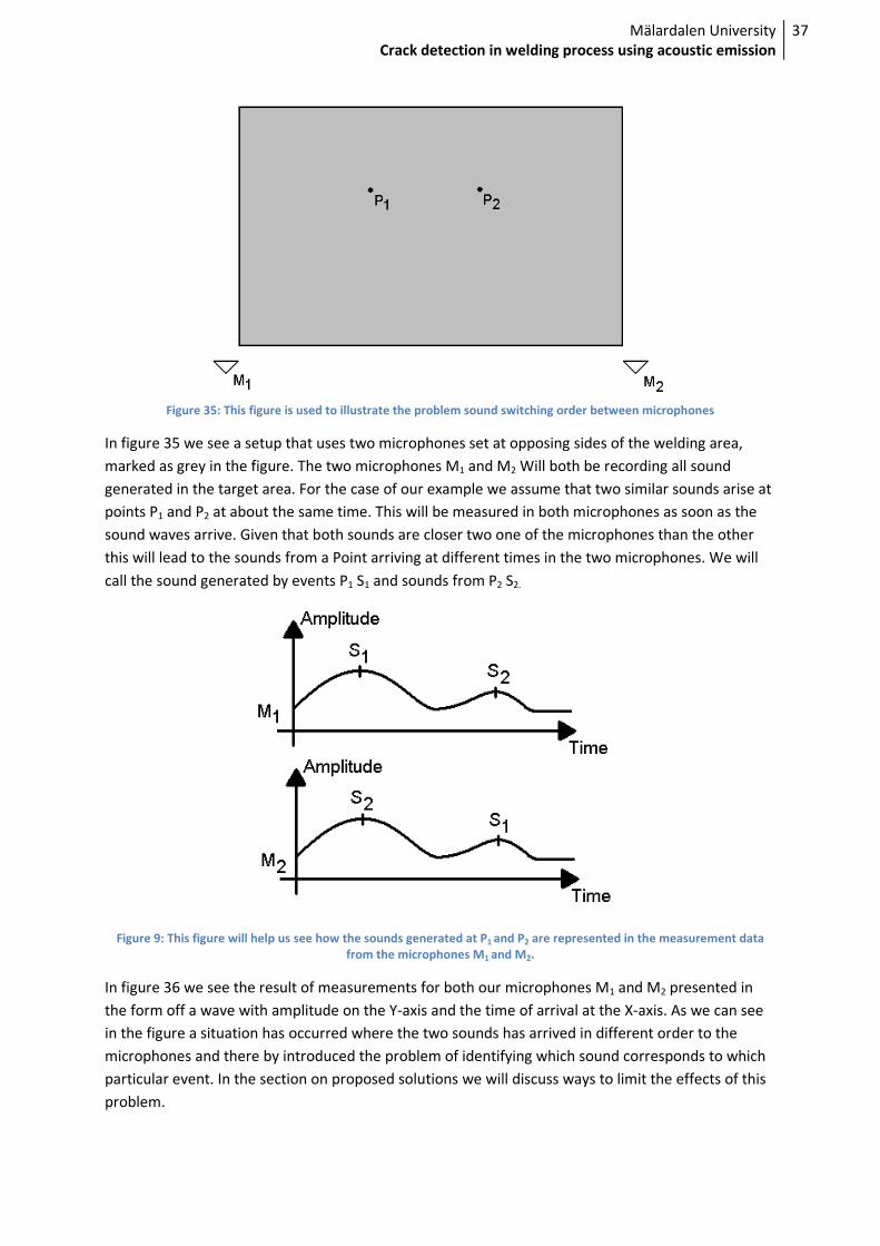
Figure 35: This figure is used to illustrate the problem sound switching order between microphones
In figure 35 we see a setup that uses two microphones set at opposing sides of the welding area,
marked as grey in the figure. The two microphones M1 and M2 Will both be recording all sound
generated in the target area. For the case of our example we assume that two similar sounds arise at
points P1 and P2 at about the same time. This will be measured in both microphones as soon as the
sound waves arrive. Given that both sounds are closer two one of the microphones than the other
this will lead to the sounds from a Point arriving at different times in the two microphones. We will
call the sound generated by events P1 S1 and sounds from P2 S2.
Figure 9: This figure will help us see how the sounds generated at P1 and P2 are represented in the measurement data
from the microphones M1 and M2.
In figure 36 we see the result of measurements for both our microphones M1 and M2 presented in
the form off a wave with amplitude on the Y-axis and the time of arrival at the X-axis. As we can see
in the figure a situation has occurred where the two sounds has arrived in different order to the
microphones and there by introduced the problem of identifying which sound corresponds to which
particular event. In the section on proposed solutions we will discuss ways to limit the effects of this
problem.

Mälardalen University
Crack detection in welding process using acoustic emission
38
Microphone arrays
We started out with a lot of theoretical work in considering different approaches to designing our
microphone array. We arrived at the problem, described in the problem section, of sounds arriving in
different order to different microphones and began work with trying to figure out how to design an
array where this is less likely to happen.
Designs using two microphones
We began however with the basic concept of two microphones each positioned at opposite sides of
the welding area; it was by considering this design that we realized the problem of arrival time.
When considering this area the only thing we need to keep track of is the distance D between the
microphones.
Figure 37: our first attempt at array design which led to our discovery of the problem of sounds changing their order in
different microphones
The array in figure 37 was discarded due to the problem associated with it that we have described
and we started thinking on what changes could be made to this design. Still working with only two
microphones and still wanting to keep them at opposing sides of the weld we came up with the idea
of using an offset. Using an offset and a more limited weld area would let us guarantee the distance
to one of the microphones would always be greater than the distance to the other microphone, using
this design we would lessen the risk of arrival time problems. For this design we will have to know
both the distance between microphones D and the offset do which is the difference in length from
the center of the welding area. We will also have to limit the width of the welding are to insure that
the distance will always be greater to one of the microphones.
Mälardalen University
Crack detection in welding process using acoustic emission
39
Figure 38: In this figure we can see how a design could look when we use a limited weld area and a microphone off-set.
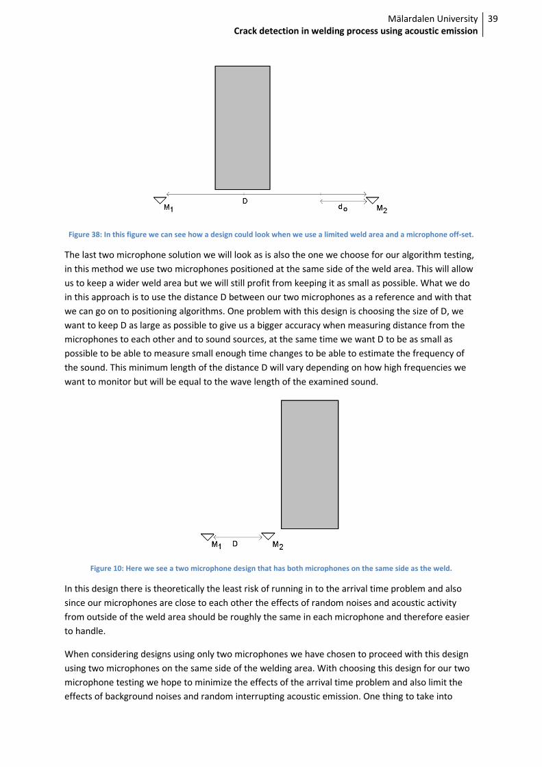
The last two microphone solution we will look as is also the one we choose for our algorithm testing,
in this method we use two microphones positioned at the same side of the weld area. This will allow
us to keep a wider weld area but we will still profit from keeping it as small as possible. What we do
in this approach is to use the distance D between our two microphones as a reference and with that
we can go on to positioning algorithms. One problem with this design is choosing the size of D, we
want to keep D as large as possible to give us a bigger accuracy when measuring distance from the
microphones to each other and to sound sources, at the same time we want D to be as small as
possible to be able to measure small enough time changes to be able to estimate the frequency of
the sound. This minimum length of the distance D will vary depending on how high frequencies we
want to monitor but will be equal to the wave length of the examined sound.
Figure 10: Here we see a two microphone design that has both microphones on the same side as the weld.
In this design there is theoretically the least risk of running in to the arrival time problem and also
since our microphones are close to each other the effects of random noises and acoustic activity
from outside of the weld area should be roughly the same in each microphone and therefore easier
to handle.
When considering designs using only two microphones we have chosen to proceed with this design
using two microphones on the same side of the welding area. With choosing this design for our two
microphone testing we hope to minimize the effects of the arrival time problem and also limit the
effects of background noises and random interrupting acoustic emission. One thing to take into

Mälardalen University
Crack detection in welding process using acoustic emission
40
account however is that when using microphones that have longer distances between each other we
can filter some background and random noise by comparing between microphones, this takes up
fairly large amount of computing power however and we much prefer to just treat these as we would
other sounds and later omit sounds that are calculated to have originated outside of the weld area.
We also look at the fact that this is the most portable solution and also one that is fairly easy to set
up. We see this as the optimal way of configuring two microphones in terms of accuracy, noise
handling and also in sorting for arrival times.
Three or more microphones
If we have the opportunity to use more than two microphones our strategy will be to build many
pairs of microphones, and also in a case of for example 3 microphones, use them as three pairs.
When setting up our microphone arrays we will also consider having different pairs of microphones
working from various angels relative to the welding are. And when we have microphones set up to
one side of the field as preferred when using two microphones we can also try different approaches
off pairing. For example we can pair microphones from different sides of the weld are and use that
data in conjunction with data obtained from a single side to get as much info as we possibly can.
The big win when using microphones from two side of the weld is that the distance between them is
greater and therefore the points for which we can decide their origin will be located with higher
precision. The drawback is as we have discussed that sounds can be wrongly matched and sounds
may end up in false positions.
Sound preprocessing
When we take a first look at recorded sound we will see that most often it comes with a few
problems that must be taken care off. Such as the sound curve being of centre, small noises, peaks
and fluctuations due to equipment and environmental factors.
To solve these issues we have constructed some tools for pre processing of sound data that will be
applied to data just before it goes to other computations, if for instance we want to use filters to
single out or remove certain frequencies that will be done before applying the methods shown in this
section. To describe our methods and show their functionality we have applied the step by step to a
test data, this data was created to be easily presented and a good example.
Mälardalen University
Crack detection in welding process using acoustic emission
41
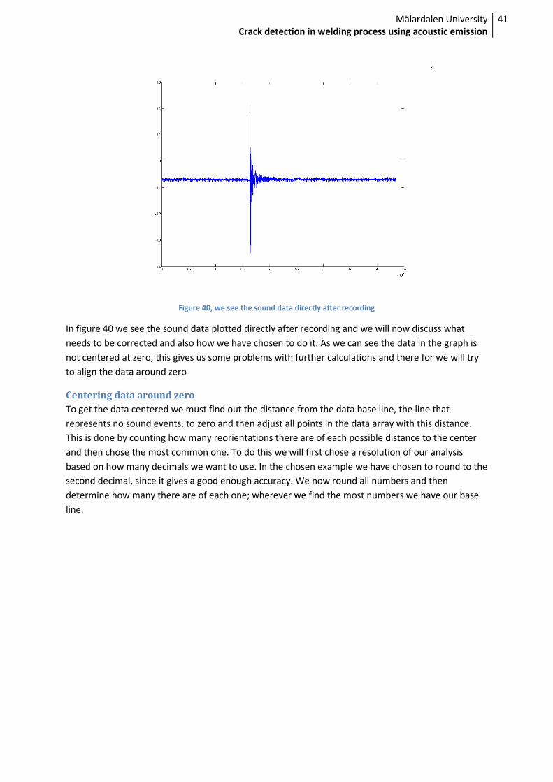
Figure 40, we see the sound data directly after recording
In figure 40 we see the sound data plotted directly after recording and we will now discuss what
needs to be corrected and also how we have chosen to do it. As we can see the data in the graph is
not centered at zero, this gives us some problems with further calculations and there for we will try
to align the data around zero
Centering data around zero
To get the data centered we must find out the distance from the data base line, the line that
represents no sound events, to zero and then adjust all points in the data array with this distance.
This is done by counting how many reorientations there are of each possible distance to the center
and then chose the most common one. To do this we will first chose a resolution of our analysis
based on how many decimals we want to use. In the chosen example we have chosen to round to the
second decimal, since it gives a good enough accuracy. We now round all numbers and then
determine how many there are of each one; wherever we find the most numbers we have our base
line.
Mälardalen University
Crack detection in welding process using acoustic emission
42
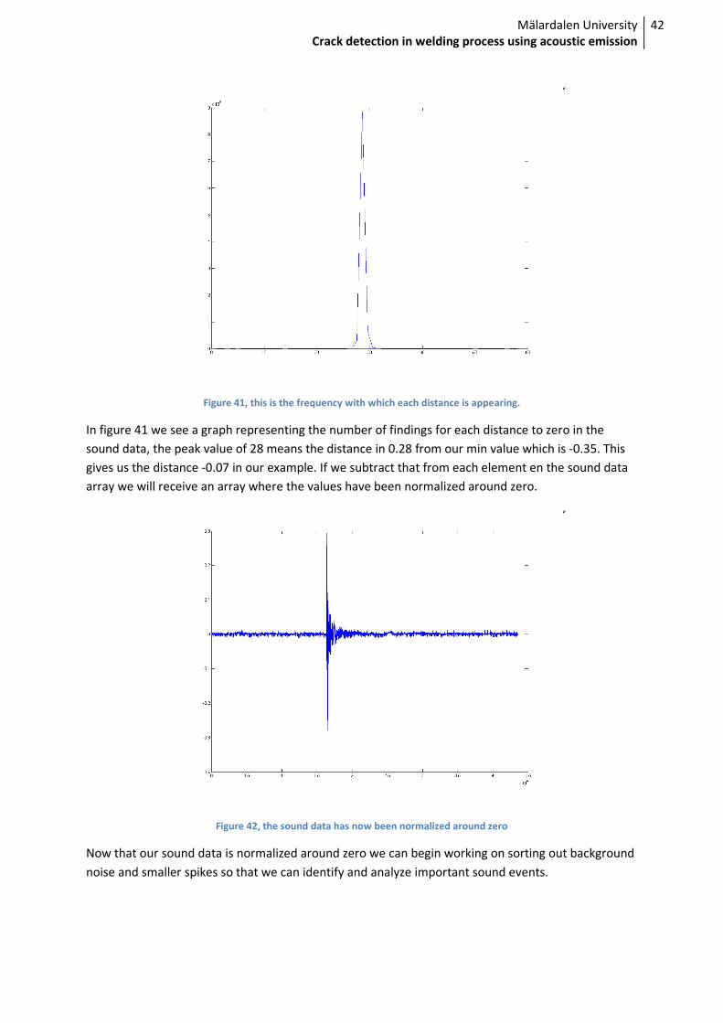
Figure 41, this is the frequency with which each distance is appearing.
In figure 41 we see a graph representing the number of findings for each distance to zero in the
sound data, the peak value of 28 means the distance in 0.28 from our min value which is -0.35. This
gives us the distance -0.07 in our example. If we subtract that from each element en the sound data
array we will receive an array where the values have been normalized around zero.
Figure 42, the sound data has now been normalized around zero
Now that our sound data is normalized around zero we can begin working on sorting out background
noise and smaller spikes so that we can identify and analyze important sound events.
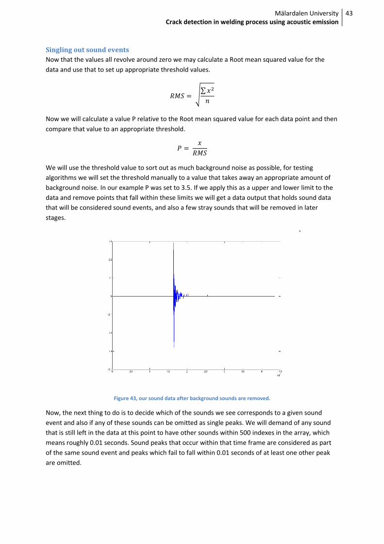
Mälardalen University
Crack detection in welding process using acoustic emission
43
Singling out sound events
Now that the values all revolve around zero we may calculate a Root mean squared value for the
data and use that to set up appropriate threshold values.
��� � �∑�
Now we will calculate a value P relative to the Root mean squared value for each data point and then
compare that value to an appropriate threshold.
� � ����
We will use the threshold value to sort out as much background noise as possible, for testing
algorithms we will set the threshold manually to a value that takes away an appropriate amount of
background noise. In our example P was set to 3.5. If we apply this as a upper and lower limit to the
data and remove points that fall within these limits we will get a data output that holds sound data
that will be considered sound events, and also a few stray sounds that will be removed in later
stages.
Figure 43, our sound data after background sounds are removed.
Now, the next thing to do is to decide which of the sounds we see corresponds to a given sound
event and also if any of these sounds can be omitted as single peaks. We will demand of any sound
that is still left in the data at this point to have other sounds within 500 indexes in the array, which
means roughly 0.01 seconds. Sound peaks that occur within that time frame are considered as part
of the same sound event and peaks which fail to fall within 0.01 seconds of at least one other peak
are omitted.

Mälardalen University
Crack detection in welding process using acoustic emission
44
Figure 44, showing our sound data with an indicator on what constitutes as one sound event.
Here we see the result off our sound event localization technique. The positive flank in the green line
marks the beginning of the sound event and the negative flank marks the end. These two points are
what we need to locate the sound when we want to use it for various calculations.
Finding a max point to use in calculations
The next thing to do is to try to approximate a max point to use for later calculations. The problem
we face here is the phenomena explained as waves in waves. That is, sound waves of various
frequencies that lies within each other and thereby makes our approximations more complex. We
might also get a good approximation by using the max point within the timeslot though this will
require that our sampling rate is big enough.
When approximate the max value we will also look at the negative values since max points might be
found amongst them as well. Therefore we will set all values within our timeslot to positive values by
use of the root square method. And also we will do our calculations in a new array and shed the old
indexes.
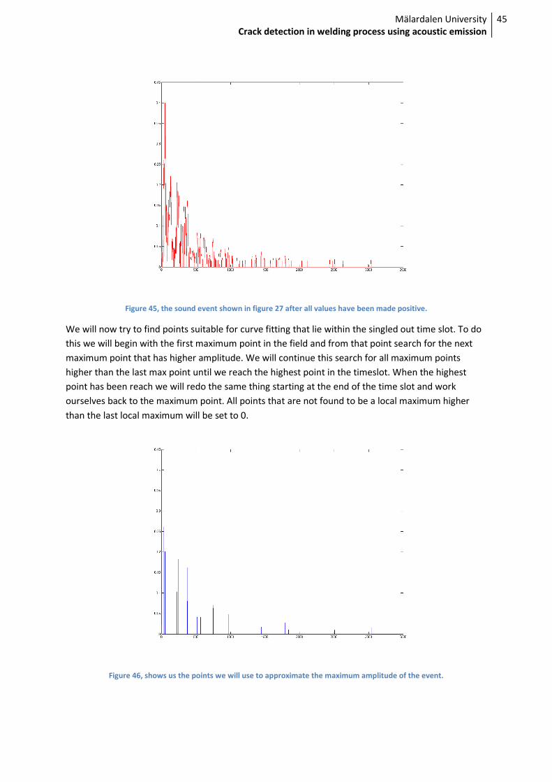
Mälardalen University
Crack detection in welding process using acoustic emission
45
Figure 45, the sound event shown in figure 27 after all values have been made positive.
We will now try to find points suitable for curve fitting that lie within the singled out time slot. To do
this we will begin with the first maximum point in the field and from that point search for the next
maximum point that has higher amplitude. We will continue this search for all maximum points
higher than the last max point until we reach the highest point in the timeslot. When the highest
point has been reach we will redo the same thing starting at the end of the time slot and work
ourselves back to the maximum point. All points that are not found to be a local maximum higher
than the last local maximum will be set to 0.
Figure 46, shows us the points we will use to approximate the maximum amplitude of the event.
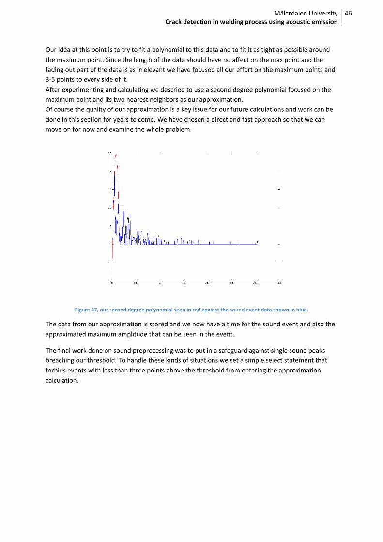
Mälardalen University
Crack detection in welding process using acoustic emission
46
Our idea at this point is to try to fit a polynomial to this data and to fit it as tight as possible around
the maximum point. Since the length of the data should have no affect on the max point and the
fading out part of the data is as irrelevant we have focused all our effort on the maximum points and
3-5 points to every side of it.
After experimenting and calculating we descried to use a second degree polynomial focused on the
maximum point and its two nearest neighbors as our approximation.
Of course the quality of our approximation is a key issue for our future calculations and work can be
done in this section for years to come. We have chosen a direct and fast approach so that we can
move on for now and examine the whole problem.
Figure 47, our second degree polynomial seen in red against the sound event data shown in blue.
The data from our approximation is stored and we now have a time for the sound event and also the
approximated maximum amplitude that can be seen in the event.
The final work done on sound preprocessing was to put in a safeguard against single sound peaks
breaching our threshold. To handle these kinds of situations we set a simple select statement that
forbids events with less than three points above the threshold from entering the approximation
calculation.
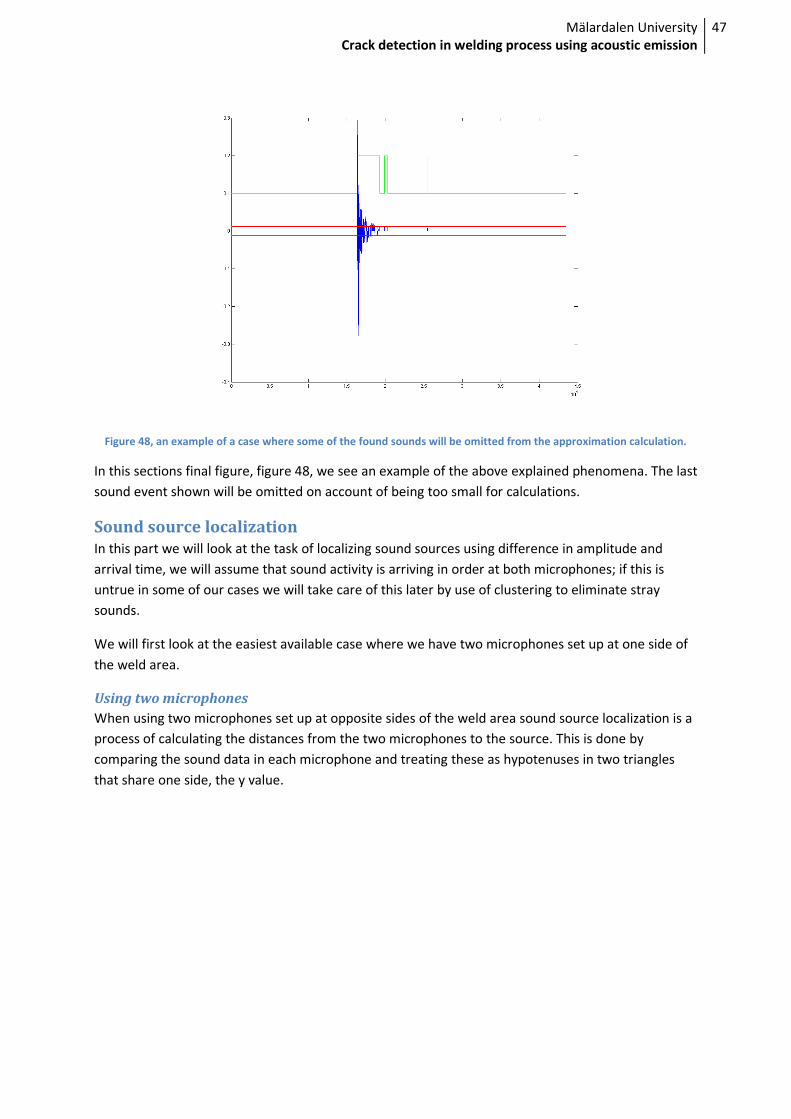
Mälardalen University
Crack detection in welding process using acoustic emission
47
Figure 48, an example of a case where some of the found sounds will be omitted from the approximation calculation.
In this sections final figure, figure 48, we see an example of the above explained phenomena. The last
sound event shown will be omitted on account of being too small for calculations.
Sound source localization
In this part we will look at the task of localizing sound sources using difference in amplitude and
arrival time, we will assume that sound activity is arriving in order at both microphones; if this is
untrue in some of our cases we will take care of this later by use of clustering to eliminate stray
sounds.
We will first look at the easiest available case where we have two microphones set up at one side of
the weld area.
Using two microphones
When using two microphones set up at opposite sides of the weld area sound source localization is a
process of calculating the distances from the two microphones to the source. This is done by
comparing the sound data in each microphone and treating these as hypotenuses in two triangles
that share one side, the y value.
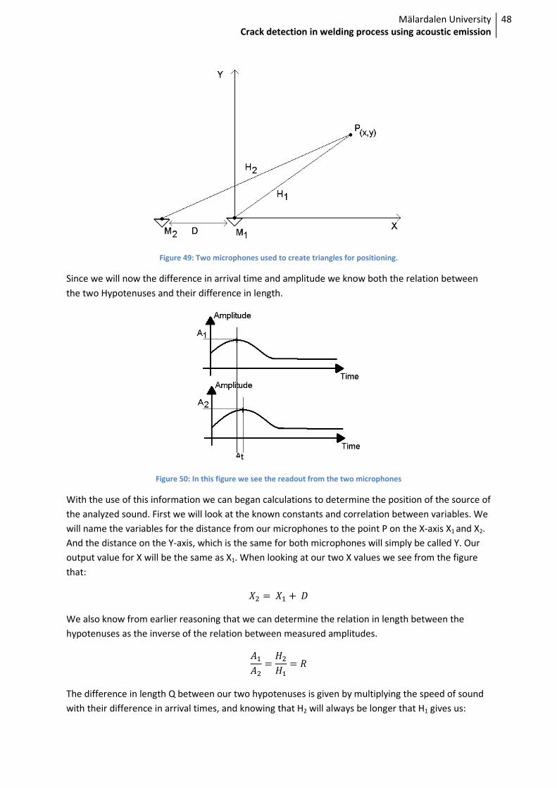
Mälardalen University
Crack detection in welding process using acoustic emission
48
Figure 49: Two microphones used to create triangles for positioning.
Since we will now the difference in arrival time and amplitude we know both the relation between
the two Hypotenuses and their difference in length.
Figure 50: In this figure we see the readout from the two microphones
With the use of this information we can began calculations to determine the position of the source of
the analyzed sound. First we will look at the known constants and correlation between variables. We
will name the variables for the distance from our microphones to the point P on the X-axis X1 and X2.
And the distance on the Y-axis, which is the same for both microphones will simply be called Y. Our
output value for X will be the same as X1. When looking at our two X values we see from the figure
that:
� � � � �
We also know from earlier reasoning that we can determine the relation in length between the
hypotenuses as the inverse of the relation between measured amplitudes.
� � � �� � �
The difference in length Q between our two hypotenuses is given by multiplying the speed of sound
with their difference in arrival times, and knowing that H2 will always be longer that H1 gives us:
Mälardalen University
Crack detection in welding process using acoustic emission
49
� �� � � � � ∆� � �
In this equation c represents the speed of sound. Knowing this we can now set up a simple equation
system to give us the length of each of our hypotenuses. Solving for H2 in both our equations gives us
two equations:
� � � � �
� � � � �
Putting these two together it is possible to calculate the value of H1:
� � � � � � �
� � � � � � �
� �� � 1� � �
� � ��� � 1� Now that we have calculated the value of H1 we can use that in any of our first two equations to
calculate H2. When this is done we can go on to the actual task of identifying that position in terms of
X and Y values of the point P. As we already know the relation between X1 and X2 and also that the
two triangles share one side it is possible to create a new equation system to solve for the reaming
unknown variables. The system will consist of these equations which we also show with the proper
values having been solved out:
� � � � �
� � � � � �� � � � � �
� � � � � We will now put these three together in the first equation to solve for X1:
� � � � � � �� � ��
� � � �� � � � 2�� � �
� � ��2�� � �
� � � �� � �2�
We can now calculate the value of X1 and use it in the first equation to calculate the value of Y. We
now have the full set off position coordinates for P.
As we see, calculating the position of P using two microphones consists of identifying relationship
between the distances from point P for both microphones and combining this knowledge with some
prior knowledge about the relation between microphones on the X-axis. This gives us a rather simple

Mälardalen University
Crack detection in welding process using acoustic emission
50
equation system to solve. When this is done we have identified the point P which is the point where
the examined sound originated.
Testing algorithms
We will now test our localization algorithms on some test data that we created by use of a stereo
microphone, a ball pen, a ruler and some paper. We recorded a sound at a set distance from the
microphone and will now try our algorithms for sound source localization on it. The same sound is
also used to illustrate and show our sound preprocessing techniques, tough in that case we only
looked at one channel at a time.
Figure 51, the two sound data sets shown at the same time.
The first thing to do now is to put both our sound data sets through the sound preprocessing. When
we do this we will be able to see how they relate to each other in terms of number of sound events
and their respective behaviors.
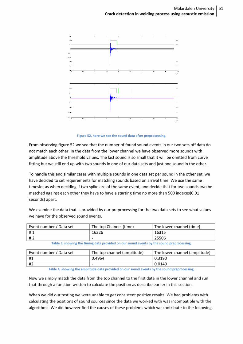
Mälardalen University
Crack detection in welding process using acoustic emission
51
Figure 52, here we see the sound data after preprocessing.
From observing figure 52 we see that the number of found sound events in our two sets off data do
not match each other. In the data from the lower channel we have observed more sounds with
amplitude above the threshold values. The last sound is so small that it will be omitted from curve
fitting but we still end up with two sounds in one of our data sets and just one sound in the other.
To handle this and similar cases with multiple sounds in one data set per sound in the other set, we
have decided to set requirements for matching sounds based on arrival time. We use the same
timeslot as when deciding if two spike are of the same event, and decide that for two sounds two be
matched against each other they have to have a starting time no more than 500 indexes(0.01
seconds) apart.
We examine the data that is provided by our preprocessing for the two data sets to see what values
we have for the observed sound events.
Event number / Data set The top Channel (time) The lower channel (time)
# 1 16326 16315
# 2 - 25506 Table 3, showing the timing data provided on our sound events by the sound preprocessing.
Event number / Data set The top channel (amplitude) The lower channel (amplitude)
#1 0.4964 0.3190
#2 - 0.0149 Table 4, showing the amplitude data provided on our sound events by the sound preprocessing.
Now we simply match the data from the top channel to the first data in the lower channel and run
that through a function written to calculate the position as describe earlier in this section.
When we did our testing we were unable to get consistent positive results. We had problems with
calculating the positions of sound sources since the data we worked with was incompatible with the
algorithms. We did however find the causes of these problems which we contribute to the following.

Mälardalen University
Crack detection in welding process using acoustic emission
52
• We had a fixed distance between our microphones that was far too small. This was due to
the construction of the stereo microphone we used and therefore beyond our control. We
did not have time and resources to acquire a new microphone due to testing being
scheduled at the end of the project.
• Our approximations on max points within sound events might be a little too inaccurate,
though this should not be given too much weight.
• We used a standard microphone and also standard software to do our testing and face some
problems with time resolution. This lead to problems with distances being too small and our
equipment not exact enough to give the necessary precision in measurements then passed
on to calculations.
We did however see some positive results and saw enough coherencies to validate our calculations.
We hope to continue our work with testing out our algorithm using more precise measurement
equipment and more favorable situations.
Sound data handling and clustering
When the position of the source of each off our registered sound events have been calculated we
save the data as coordinate information. Given this information we can make numerous types of
presentations of the data such as, plotting all points as a representation of the welding area or focus
on certain areas or sounds of certain amplitudes.
When it comes to strategies of clustering there are different ways to go about the task. We have
considered two different approaches. One discrete focusing on sorting our events based on their
position and another less discrete method focusing on amplitude and position relative to other
events.
First approach
In this approach what we do is simply to divide our weld area into fields off a set appropriate size,
and the simply add to value to fields which holds many points. In this approach we go through all
coordinates that we have gathered from sound data and allocate a point to the area from where it
came. In the end we have a field matrix representation of the welding area that has higher points
where there are many sound generating events. Here the size of our fields and the number of fields
decide the resolution of our clustering process.
We can then omit fields that have none or few points and focus our attention on areas where there
are higher points.
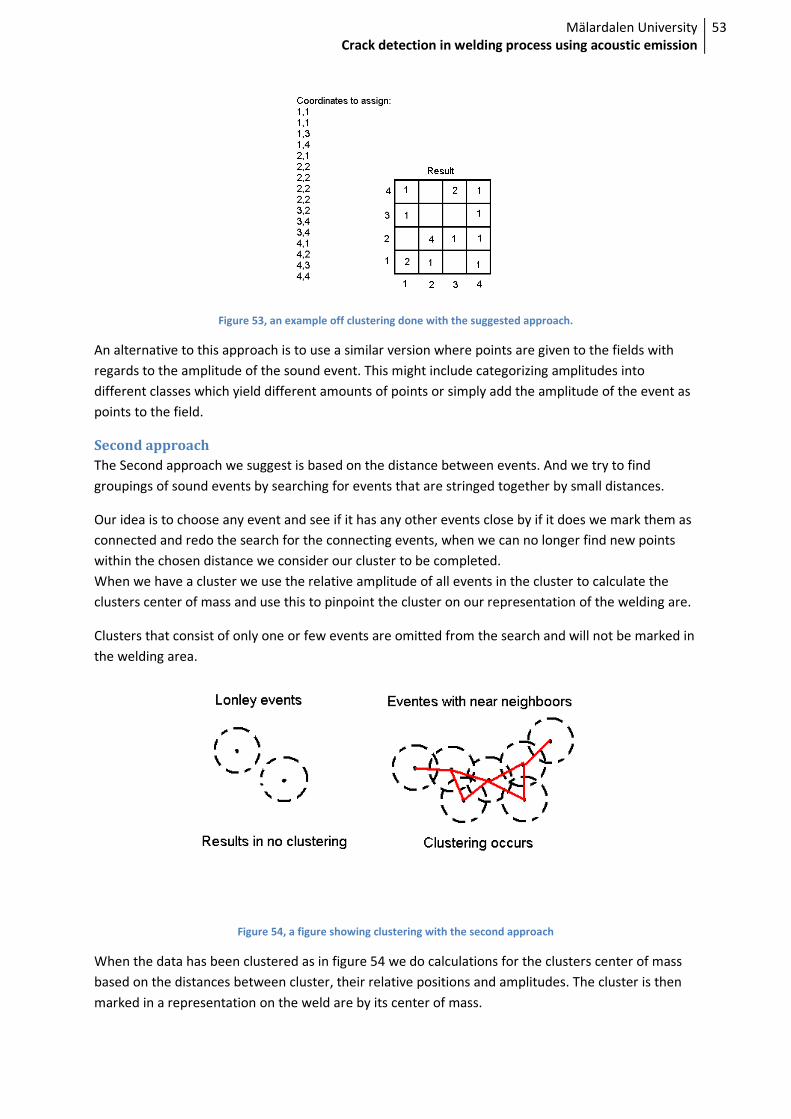
Mälardalen University
Crack detection in welding process using acoustic emission
53
Figure 53, an example off clustering done with the suggested approach.
An alternative to this approach is to use a similar version where points are given to the fields with
regards to the amplitude of the sound event. This might include categorizing amplitudes into
different classes which yield different amounts of points or simply add the amplitude of the event as
points to the field.
Second approach
The Second approach we suggest is based on the distance between events. And we try to find
groupings of sound events by searching for events that are stringed together by small distances.
Our idea is to choose any event and see if it has any other events close by if it does we mark them as
connected and redo the search for the connecting events, when we can no longer find new points
within the chosen distance we consider our cluster to be completed.
When we have a cluster we use the relative amplitude of all events in the cluster to calculate the
clusters center of mass and use this to pinpoint the cluster on our representation of the welding are.
Clusters that consist of only one or few events are omitted from the search and will not be marked in
the welding area.
Figure 54, a figure showing clustering with the second approach
When the data has been clustered as in figure 54 we do calculations for the clusters center of mass
based on the distances between cluster, their relative positions and amplitudes. The cluster is then
marked in a representation on the weld are by its center of mass.

Mälardalen University
Crack detection in welding process using acoustic emission
54
Crack recognition and localization Hypothesis
Our theory concerning the detection on localization of cracks and other related events in the
material is to some extent inspired by the work by A. N. Ser’eznov, L. N. Stepanova, E. Yu. Lebedev, S.
I. Kabanov, V. N. Chaplygin, S. A. Laznenko, K. V. Kanifadin, and I. S. Ramazanov[3].
As in their work we want to use information given by our multi sensor system to calculate the
locations of all sound generating events and then use different clustering methods to gain
information about what goes on in the material. We want to track different types of sound events
and use different clustering strategies to try to get as much useful information as possible.
We also believe that different clustering and analysis methods may give new information on the
same data, one strategy might detect cracks while one might detect welds not cooling properly in
other ways.
What we need to do now is improve our hypotheses by beginning work on recording done with
multiple microphones and start evaluating different clustering approaches and also the analysis tools
used to interpret results from clustering.
Results
After examining the data from Volvo we arrived at a split decision, either the presence of spikes are
not coherent with the presence of cracks or they are in which case some recordings from the first
data set must be discarded as false data. To better determine this we must do more measurements
and it would also help to get a grasp of how much time has been allowed between welds.
According to A. N. Ser’eznov, L. N. Stepanova, E. Yu. Lebedev, S. I. Kabanov, V. N. Chaplygin, S. A.
Laznenko, K. V. Kanifadin, and I. S. Ramazanov[3] the cool down time for a weld is somewhere
around 10 minutes long and sounds will be generated throughout the whole cool down period. This
means that sounds generated in the end of one welds cool down might interfere with the recording
of another weld. To prevent this we must allow enough time between welds so that sound
generating activity is only taking place in the weld that we want to examine.
Since the sensitivity of the equipment was changed during the recording of the first data set it is
possible that spikes belonging to another weld were recorded in the non cracked data at such high
amplitude.
From the theoretical work our result is a set of algorithms and methods that will preprocess and do
calculations in sound data. The algorithms did not do well in our initial tests but too many
parameters in the test were unfavorable and some measurements done on the equipment where
inaccurate.

Mälardalen University
Crack detection in welding process using acoustic emission
55
Conclusions and Future work
We will conclude that there is a strong relationship between sound activity occurring at around 150-
200 KHz and changes taking place in the material. Spikes and similar events will be considered as
indications for events taking place inside the cooling materials as long as the spikes occur in
conjunction with a rise in noise at the specified frequency.
We also conclude that experiments must continue and that we need more data to solidify our
theories and also that we will want to use multichannel recording devices so that we can gather
more data from our welds and also try to locate the sources of spikes and other occurrences that we
observe in our data.
We want to keep up experiments at Volvo and keep doing calculations and examinations on the data,
we also want to start development on our localization techniques and gather data to use with our
clustering theory to see how much data can be gathered in this fashion.
We want to explore the field of air transmitted emission and see if we can get data in this way, if that
is possible there is vast potential for development of small hand held devices that can help us control
weld quality, both in industrial environments and in home environments.
The first step of our future work is to gather more data in the same way as we obtained data set 1
and 2 and strive for even more similar procedures for all the welds done in these experiments. We
also want to do measurements over an extended period of time for one single weld to see for how
long it will emit sounds so that we can improve our experiments and reduce that risk of welds
interfering with one another.
We also want to start working with multichannel systems and therefore we want to gather data that
will allow us to get started in that field.
Summary
In this rapport we examined the data provided by Volvo recorded from actual welds in their
laboratory. The data was divided into two sets with the second one being done after initial testing
was performed on the first one which led to some differences in method. We made some interesting
observations in the data and found spikes and noises that might indicate events inside the material.
We had a large section on sound data handling where we also covered how we might track changes
in the material through acoustic emission. We looked at algorithms for sound preprocessing and
sound source location. We also discussed clustering and our theories on how to use the acquired
data to find cracks and other defects within the material.
We finished the rapport with a conclusion and suggestions for future work. The conclusion made
where that given the provided data we lean against a theory where the spikes observed in the
acoustic data do indicate cracks but that we will need more data to confirm this and that we also
need to understand how some of the recording that were made that go against this theory came
about.
Mälardalen University
Crack detection in welding process using acoustic emission
56
Referenses
[1] Baifeng JI*, Weilian QU, “The Research of Acoustic Emission Techniques for Non Destructive
Testing and Health Monitoring on Civil Engineering Structures!”, Hubei Key laboratory of
Roadway Bridge&Structure Engineering., Wuhan University of Technology, Wuhan 430070, China
[2] C.E. Hartbower, W.G. Reuter, C.F. Morais and P.P. Crimmins. “Use of Acoustic Emission for
the Detection of Weld and Stress Corrosion Cracking”. Acoustic emission STP 505, American
society for Testing and Material 1972.
[3] A. N. Ser’eznov, L. N. Stepanova, E. Yu. Lebedev, S. I. Kabanov, V. N. Chaplygin, S. A.
Laznenko, K. V. Kanifadin, and I. S. Ramazanov. “Acoustic-Emission Study of the Possibilities
of Localizing Flaws of a Welded Joint during Cooling”. Chaplygin Siberian Research Institute of
Aviation, ul. Polzunova 21, Novosibirsk, 630051 Russia Received November 17, 2008
[4] E. D. Di Claudio, R. Parisi and G. Orlandi, “MULTI-SOURCE LOCALIZATION IN REVERBERANT
ENVIRONMENTS BY ROOT-MUSIC AND CLUSTERING”, INFOCOM Dpt. University of Rome “La
Sapienza” Via Eudossiana 18,I-00184 ROMA RM Italy
[5] Ming Jaan, Alex C. Kot, Meng H. Er, “PERFORMANCE STUDY OF TIME DELAY ESTIMATION IN A ROOM ENVIRONMENT”, Centre for Signal Processing School of Electrical and Electronic
Engineering Nanyang Technological University, Nanyang Avenue, Singapore 639798
[6] Brent C. Kirkwood, “Acoustic Source Localization Using Time-Delay Estimation”, Technical
University of Denmark, August 4, 2003
Appendix A, Matlab
Instructions for using this Appendix
This appendix consists of a number of Matlab .m-files. To use them as intended follow the following
steps:
1. Load appropriate sound data into a variable called data. Appropriate sound data means data
recorded using two parallel channels(Stereo)
2. Copy the entire code of the file Preprocessing.m and paste it at the end of itself, then make
the following changes to it:
at line 9 change: A=data(:,1); into A=data(:,2);
at line 339 change Top_Channel_Time = Event_time; into Low_Channel_Time = Event_time;
at line 340 change Top_Channel_Amp = Event_peak; into Low_Channel_Amp = Event_peak;
3. Run Preprocessing.m
4. You now have the data you need for position calculation in the variables
Low_Channel_time, containing event times for channel B
Top_Channel_time, containing event times for channel A
Low_Channel_Amp, containing event amplitudes for channel B
Top_Channel_Amp, containing event amplitudes for channel A
5. Run Get_coordinates.m

Mälardalen University
Crack detection in welding process using acoustic emission
57
6. Examine your result in Pos_X and Pos_Y, two vectors containing the coordinates for found
points listed in chronological order.
Preprocessing.m % all Matlab code for the sound preprocessing, if you mean to use this % code, read through the instructions in: Appendix Matlab code clear Top_channel_Time; %clear these for reruns of the program
clear Top_channel_Amp; clear Event_time; clear Event_peak;
A=data(:,1);% this whole section is run twice in this M-file, the second
run is omitted from appendix % second run: A=data(:,2); % the ending part where the data is saved at line 320 and 321 % is also altered in the second run
%The first step is to find max and min in the array made up by sound data, %multiply these with our resolution and round them.
resolution = 100; %100 means second decimal Ma = max(A); Mi = min(A);
Ma = Ma*resolution; Mi = Mi*resolution;
Ma = round(Ma); Mi = round(Mi);
size_F = Ma - Mi; %determines the size of the field used to count
frequencies.
%create an array of the the appropriate size with indexes from 1..X
%This array will be used to find out which values are most common in the %examined sound and thereby find the base level from which the sound data %oscillates. clear Freq_field; Freq_field(size_F+1) = 0;
%for all elements: %multiply by a hundred, round and subtract the min value to get x %add one to the array index(x+1).
%First we get the size of A size_A_vec= size(A); size_A = size_A_vec(1);
for ind=1:size_A, x = A(ind); x = round(resolution*x) - Mi;
Mälardalen University
Crack detection in welding process using acoustic emission
58
Freq_field(x+1) = Freq_field(x+1) +1; end
[C,I] = max(Freq_field); %now we find out which index(distance) that has gotten most "votes".
distance = (Mi + I-1)/resolution; B=A; for ind=1:size_A, B(ind)=B(ind)-distance; end
%output is stored in an array called B %B contains the data from array A recalculated to oscillate a lot closer to %0.
MaZ = B; size_MaZ = size_A; %we have an array around zero and want upper and lower thresholds.
%the Array is called MaZ and its known size is in size_MaZ sum = 0; for ind=1:size_MaZ, % here we do! x=MaZ(ind); x = x^2; x = sqrt(x); sum = sum + x; end %to calculate treshold values we will use the formula for peaks relative to %rms.
%Xf=P/RMS formula for calculating the threshold.
%we will set a certain value for Xf. % we are looking for RMS*X where Xf is the factor, Xf = 3.50; % value chosen to fit the problem and give manageable data. % this value gives a simple curve for trying out our further solutions and % algorithms. for ind=1:size_MaZ, Upper_T(ind) = Xf*(sum/size_MaZ); Lower_T(ind) = Xf*((sum/size_MaZ)*-1); end
%now we have the values for our threshold stored in an array matching %indexes so that we can plot them in nice understandable graphs hold off subplot(2,2,1); plot(A)
%Also plots the field where we counted the number of entries per value so %that we can see it and get a better feel for it. subplot(2,2,2); plot(Freq_field) subplot(2,2,3); plot(B)
%here we create and array that we will use later when plotting found sound
Mälardalen University
Crack detection in welding process using acoustic emission
59
%activity: Activity = MaZ;
% this loop exists to set all sound events that do not clear our threshold % values to 0. for ind=1:size_MaZ, activity(ind)=0; if MaZ(ind) < Upper_T(ind) && MaZ(ind) > Lower_T(ind) MaZ(ind) = 0;
end end %Now we plot our trimmed data with the thresholds plotted in red subplot(2,2,4); hold off plot(MaZ) hold on plot(Upper_T,'Color','red') plot(Lower_T,'Color','red')
%now we shall figure out where we have sound activity, that is where we %should apply our analytic tools.
%In the activity array values are paired giving the first and last index in %each sound event.
%copy for plotting, this is only here to help make understandable plots plot_act = activity;
activity_p = 1; % is an activity array pointer(pointing at where data
should go)
found = 0; %variables for finding activity. has_length = 0;
%describing this loop: %The point of this loop is two move through the data until it finds %activity over the threshold(any non 0 value). When this is found it shall %search for further values and see which corresponds to the same event. %An event is considered over when more than 500 indexes has passed since %last activity(at our Sampling rate of ~44KHz this means around 0.01 %seconds). %the loops should also exclude sounds that are alone for 500 indexes in any %direction. for ind=1:size_MaZ, if MaZ(ind)==0 && found==0 %no sound
elseif MaZ(ind)~=0 && found==0 %found sound from no sound found = 1; activity(activity_p) = ind; activity_p = activity_p + 1; elseif MaZ(ind)~= 0 && found==1 && has_length==0 if ind - activity(activity_p-1) > 500 %single peak, no find activity_p = activity_p-1; found = 0; else %found something activity(activity_p)=ind; has_length = 1; end

Mälardalen University
Crack detection in welding process using acoustic emission
60
elseif MaZ(ind) ~= 0 && found ==1 && has_length ==1 %gives two cases, either it’s the end of previous sound or the
beginning %of a new one
if ind - activity(activity_p) > 500 %compares against end of sound %means its a new sound has_length = 0; activity_p = activity_p+1; activity(activity_p) = ind; activity_p = activity_p + 1; %now it is ready to examine the sound as if it were a new one else activity(activity_p) = ind; end else
end
end
% now we want to make it plot able in some nice and understandable way
using % plot_act found = 0; activity_p =1; nr_of_s = 0;
%This only makes a plot able line that is high when we are inside a sound %event and then it is low when we are outside of registered sound events. for ind=1:size_MaZ, if ind < activity(activity_p) && found ==0 % no activity plot_act(ind) = 0.1; elseif ind == activity(activity_p) && found == 0 %start of activity nr_of_s = nr_of_s +1; %record new sounds found = 1; activity_p = activity_p+1; plot_act(ind) = 0.2; elseif ind < activity(activity_p) && found ==1 plot_act(ind) = 0.2; elseif ind == activity(activity_p) && found == 1 found = 0; activity_p = activity_p+1; plot_act(ind) = 0.1; else plot_act(ind) = 0.1; end end
%Here we plot the line that shows us where we have activity. plot(plot_act,'Color','green')
%sound events now have begginings and ends.
%both will be created when needed
% we study all sounds one by one to determine their peaks and also their
Mälardalen University
Crack detection in welding process using acoustic emission
61
% times(times will be their start times).
%To place them in correct order we will need a peak index, showing where to %put information calculated from the currently examined peak. Peak_index = 1; %points initially to the first index.
for ind=1:nr_of_s, Event_start = activity(ind*2 -1); Event_end = activity(ind*2); Event_array = MaZ(Event_start:Event_end); %copys the data from within
the time slot to a new array.
for index=1:size(Event_array), Event_array(index) = sqrt(Event_array(index)^2); end %Event array now only contains positive values
%here is where we mark the points that are both local maximum points and
higher than the proceeding point. %We begin with the first point and move on until we find a point that is %both a local max point and higher than the start point, we den redo %this from the new point and keep on until we reach the maximum point.
%this is then done once again in reverse form the end of the data field.
%we begin by saving the index for the whole intervals maximum point [Toss,Glob_Max] = max(Event_array); %we define a target array(we might as well just keep the points but %this helps in showing our results Found_points = Event_array; Found_points(1) = Event_array(1); % loads the first point into the
array %and a variable to save the amplitude of the last maximum point. Last_amp = Event_array(1); %This loops goes from first index to global maximum for index=2:Glob_Max, % begins at the second index since the first index
is atomically a max point %first we find out if what we see is a max point if Event_array(index-1) < Event_array(index) && Event_array(index+1)
< Event_array(index) %we have a max point if Event_array(index) > Last_amp Last_amp = Event_array(index); Found_points(index) = Event_array(index); else Found_points(index) = 0; end else Found_points(index) = 0; end end
%Now we are to reset our variables to search for the other way around %first we set the last point size_Event_array_vec= size(Event_array); End_point = size_Event_array_vec(1); Found_points(End_point) = Event_array(End_point); %we then set Last_amp to that point: Last_amp = Event_array(End_point); %now we set the end point for our loop

Mälardalen University
Crack detection in welding process using acoustic emission
62
Loop_end_index = End_point - Glob_Max; %for convenience we also store the size of the array in a variable
%now we loop for index=1:Loop_end_index, % begins at the second index since the
first index is atomically a max point %first we find out if what we see is a max point Act_index = End_point-index; if Event_array(Act_index+1) < Event_array(Act_index) &&
Event_array(Act_index-1) < Event_array(Act_index) %we have a max point if Event_array(Act_index) > Last_amp Last_amp = Event_array(Act_index); Found_points(Act_index) = Event_array(Act_index); else Found_points(Act_index) = 0; end else Found_points(Act_index) = 0; end end
%to continue with curve plotting we shall arrange our points into two %vectors, one for X and one for Y_values. X_Y_Vec_I = 1; clear X_values; clear Y_values; for index=1:size(Found_points), if Found_points(index) == 0; else
X_values(X_Y_Vec_I) = index; Y_values(X_Y_Vec_I) = Found_points(index); X_Y_Vec_I = X_Y_Vec_I + 1;
end end %does what its supposed to
%ensure that no stray sounds are measured if X_Y_Vec_I > 4 %code to find Max values in the two arrays and focus in on them and their %closest neighbors. [Max_in_Y,index_of_max] = max(Y_values);
low = index_of_max-1; high = index_of_max+1; TEsting = X_values; X_values = X_values(low:high); Y_values = Y_values(low:high);
p = polyfit(X_values,Y_values,2); X_vector = 1:150; clear y; y = polyval(p,X_vector); Event_max = max(y);
%Now we report on our findings: Event_time(Peak_index) = Event_start; Event_peak(Peak_index) = Event_max; Peak_index = Peak_index + 1;
Mälardalen University
Crack detection in welding process using acoustic emission
63
else end
end %This saves our findings for future calculations Top_channel_Time = Event_time; Top_channel_Amp = Event_peak;
Get_coordinates.m %Get coordinates from the Time/amplitude arrays.
%When this file is run you should have the following variables: %Low_Channel_Time, containing event times for channel B %Top_Channel_Time, containing event times for channel A %Low_Channel_Amp, containing event amplitudes for channel B %Top_Channel_Amp, containing event amplitudes for channel A
% our strategie here is a loop within a loop wich hangs at a value in the % first data set(hanging on Time values) %we then compare times with time from the other microphone, when we find %the closest value in time(that lies within 500 indexes(0.01sec)) we do our %calculations.
size_Top_vec= size(Top_channel_Time); size_Top = size_Top_vec(2)
size_Low_vec= size(Low_channel_Time); size_Low = size_Low_vec(2)
Out_put_index = 1; ind_L = 1;
for ind_T=1:size_Top, Loop_break = 0; while ind_L < size_Low && Loop_break == 0, % we will fiorst see if we have a match right of the bat
if Top_channel_Time(ind_T) - Low_channel_Time(ind_L) < 500 &&
Top_channel_Time(ind_T) - Low_channel_Time(ind_L) > -500 % they match eahother %here we will make a call to the function pos which takes the %following arguments as input: %AVin, Is the Amplitude of the microphone that is furthest away %from the weld %TVin,Time fro the microphone that is furthest away %AHin, Amplitude for the closer microphone %THin, Time for the closer microphone %din, distance between microphones in mm.
% in our data the lower channel was closer to the test sound % events. [Pos_Y(Out_put_index) Pos_X(Out_put_index)] =
pos(Top_channel_Amp(ind_T),Top_channel_Time(ind_T),Low_channel_Amp(ind_L),L
ow_channel_Time(ind_L),10); Out_put_index = Out_put_index + 1;

Mälardalen University
Crack detection in welding process using acoustic emission
64
Loop_break = 1; elseif Top_channel_Time(ind_T) > Low_channel_Time(ind_L) % case
here we need to advance the second channel so do nothing Ind_L = Ind_L + 1; else Loop_break = 1; end end end
Position.m function [y x] = pos(AVin,TVin,AHin,THin,din)
%Calculations as seen in the rapport.
AmpV = AVin; %closest microphone Amplitude TidV = TVin; %Closest microphone Time AmpH = AHin; %Furthest away microphopne Amplitude TidH = THin; %Furthest away microphopne Time d = din; %Distance between te microphones in millimeters
R = AmpV/AmpH; %amplitudes
Q = (TidH-TidV)*330/1000; %Time in nano seconds, results in millimeters
Hb = Q/(R-1) Ha = Hb*R
b = (Ha^2-Hb^2+d^2)/(2*d); a = d - b; %our x value h = sqrt(Hb^2-b^2); %our y value
x = b; y = h;
end
Related Documents