Crabgrass Frontier Revisited in New York : Through the Lens of 21st-century Data Sun Kyoung Lee ⇤ Yale University Abstract Jackson’s famous Crabgrass Frontier: The Suburbanization of the United States (1985) ar- gues that when American cities suburbanized in the early nineteenth century, the richest households moved from the core to the periphery, the poorest stayed in the core, and the households that moved to the periphery were richer than those who were there be- fore them. I study the gradual process of prewar suburbanization in America’s biggest city, New York City, between 1870 and 1940. During this time there were huge trans- portation infrastructure improvements at both intra- and inter-city level, and there was gradual suburbanization, just as in Jackson (1985). I construct a historical longitudinal database that follows individuals to analyze how the migration patterns differ across workers with different income (skills). Rich people on average did not leave the core and poor people on average did not stay. New suburbanites to the city periphery were not richer than the people who already lived at the periphery. Jackson’s fundamental claim about the growth of high income at the edge relative to the center still holds true for my study period. However, I show the mechanism behind this change and show that this relative change in income growth at the edge did not result from a simple shuffling of rich and poor. Up until the Great Depression, flows of migrants from and to outside ⇤ [email protected] 1

Welcome message from author
This document is posted to help you gain knowledge. Please leave a comment to let me know what you think about it! Share it to your friends and learn new things together.
Transcript

Crabgrass Frontier Revisited in New York :Through the Lens of 21st-century Data
Sun Kyoung Lee⇤
Yale University
Abstract
Jackson’s famous Crabgrass Frontier: The Suburbanization of the United States (1985) ar-
gues that when American cities suburbanized in the early nineteenth century, the richest
households moved from the core to the periphery, the poorest stayed in the core, and
the households that moved to the periphery were richer than those who were there be-
fore them. I study the gradual process of prewar suburbanization in America’s biggest
city, New York City, between 1870 and 1940. During this time there were huge trans-
portation infrastructure improvements at both intra- and inter-city level, and there was
gradual suburbanization, just as in Jackson (1985). I construct a historical longitudinal
database that follows individuals to analyze how the migration patterns differ across
workers with different income (skills). Rich people on average did not leave the core
and poor people on average did not stay. New suburbanites to the city periphery were
not richer than the people who already lived at the periphery. Jackson’s fundamental
claim about the growth of high income at the edge relative to the center still holds true
for my study period. However, I show the mechanism behind this change and show that
this relative change in income growth at the edge did not result from a simple shuffling
of rich and poor. Up until the Great Depression, flows of migrants from and to outside
1

the metropolitan area were the dominant force in changing average income. Richer peo-
ple from outside NYC metropolitan area migrated to the periphery and poorer people
from outside NYC metropolitan migrated to the core. The people from the city core who
left the metropolitan area were far richer than the people from the periphery who left
the metropolitan area. Furthermore, people who stayed at the periphery got richer as
the metropolis grew. Many readers have interpreted Crabgrass Frontier as the story of
America’s suburbanization always and everywhere, and so my finding that two of the
major propositions in that book and the mechanism behind income growth at the edge
do not apply to 1870-1940 New York has implications beyond local history.
JEL: N71, N72, N91, N92, O18, R3, R4, R12

1 Introduction: Crabgrass Frontier Revisited
“Our property seems to me the most beautiful in the world. It is so close to Babylonthat we enjoy all the advantages of the city, and yet when we come home we are awayfrom all the noise and dust.”1
Jackson (1985)’s Crabgrass Frontier: The Suburbanization of the United States remains one ofthe most influential books ever written on urban history and on American cities. One of themain ideas in the book is that the rich began the flight from the city first — something thatthe middle classes eventually emulated as city tax rates skyrocketed and those on the lowerend of the economic stratum moved into the city.
Jackson (1985) found that suburbanization, a phenomenon that started no later than theearly 19th century, was accompanied by enormous growth in metropolitan size and rapidpopulation growth on the periphery, an absolute loss of population at the center, and anincrease in the average journey to work, and a rise in the socioeconomic status of suburbanresidents.
However, Jackson did not have the benefit of the datasets and quantitative analysis tech-niques that we have now. In particular, he could not follow individuals. He could observe,for instance, that suburbs gained population and that the central parts of cities lost popula-tion, but he did not know whether any individual moved from the city to the suburb. Withonly periodic snapshots of aggregates and no guarantee that anyone in any snapshot is inany other, we cannot begin to think how events affected individuals. While formal welfareanalysis is beyond the scope of the current paper, the longitudinal analysis that I performhere is a necessary prologue to any such work.
My study period (1870-1940) occurs after Jackson’s study (i.e. 1815-1875) and before themajor introduction of highways in the US (Baum-Snow (2007)). I concentrate on New YorkCity. I investigate three of the major conclusions of Crabgrass Frontier:
1. That the relative population of more suburban areas increased
2. That the richest people were the ones who led the movement from the center of thecity to the periphery, and poor people stayed in the center of the city
1Jackson (1985) cites the letter in cuneiform on a clay tablet, which was a letter to the King of Persia in539 B.C.. Jackson (1985) argues Boston, Philadelphia, and New York established suburbs well before theRevolutionary War, and this letter represents the first extant expression of the suburban ideal.
3

3. That the people who moved from the center to the periphery were richer than thepeople living in the periphery
I investigate each of these propositions in turn. Notice that second and third propositionsare explicitly longitudinal statements that repeated cross-section data cannot examine.
To bring Jackson’s work to the 21st century, I create a micro longitudinal database ofindividuals by linking US demographic census records. These new datasets provide a veryhigh level of geographic resolution and help shed light on the evolution of neighborhoodsover a long time horizon as transportation infrastructure was developed. I link individual-level US demographic census records from 1870 to 1940 (every decade, except for 1890 asthe 1890 population census was lost due to fire), to track individuals’ residential locations inrelation to transit infrastructure-driven transit access change. I decompose how neighbor-hood changes were driven by out-migration and in-migration of individuals with differentsocioeconomic characteristics, along with the incumbents’ income increase when intra-citytransit infrastructure improved market access.
Through the above approach, I “let the data speak” about the process of suburbanizationin the biggest city in America. Regarding Jackson’s three points, I find
1. Yes, population decentralized
2. No, the people who stayed in the center of the city were richer than the ones who leftthe city center
3. No, the people who moved to the periphery were poorer than the people alreadyliving there
4. Relatedly, richer people from outside NYC metropolitan area migrated to the periph-ery and poorer people from outside NYC metropolitan area migrated to the core; thepeople from the city core who left the NYC metropolitan area were far richer than thepeople from the periphery who left the metropolitan area; furthermore, people whostayed at the periphery got richer as the metropolis grew.
Jackson’s fundamental claim about the growth of high income at the edge relative to thecenter still holds true for my study period. However, I show the mechanism behind this
4
change and show that this relative change in income growth at the edge did not result froma simple shuffling of rich and poor.
Up until the Great Depression, flows of migrants from and to outside the metropolitanarea were the dominant force in changing average income. Richer people from outsideNYC metropolitan area migrated to the periphery and poorer people from outside NYCmetropolitan migrated to the core. The people from the city core who left the metropolitanarea were far richer than the people from the periphery who left the metropolitan area.Furthermore, people who stayed at the periphery got richer as the metropolis grew.
To be sure, I am studying only one city for one period, and it is a period outside Jack-son’s explicit study period. But the city is America’s largest, and the period encompassesNew York’s greatest growth and most dramatic change. Many readers have interpretedCrabgrass Frontier as the story of America’s suburbanization always and everywhere, andso my finding that two of the major propositions in that book and the mechanism behindincome growth at the edge do not apply to 1870-1940 New York has implications beyondlocal history.
Several research projects explain the central city population decline. For example, Baum-Snow (2007) demonstrates that the construction of new limited-access highways causedcentral city population decline. Boustan (2010) focuses on sorting where white householdsleft central cities due to racial preferences. Relative to the aforementioned papers, I usea panel data of individuals that enables me to decompose the relative magnitudes of theflows among entrants, leavers and stayers and its associated income differences.
This paper also relates to the large reduced-form empirical literature on transport infras-tructure, including Banerjee et al. (2012), Baum-Snow (2007), Donaldson (2010), Donaldsonand Hornbeck (2013), Faber (2013), Duranton et al. (2013), Michaels (2008). This paper alsocontributes to the literature on the internal structure of the city, through a quantitative anal-ysis of economic geography. While there has been extensive development of economic ge-ography in the past few decades (Fujita and Ogawa (1982), and Lucas and Rossi-Hansberg(2002)), there is growing empirical literature. Especially, the structural estimation approachhas been implemented in studying the allocation of economic activity, including Ahlfeldtet al. (2012), Allen and Arkolakis (2013), Allen et al. (2015), Heblich et al. (2018), Monte et al.(2015), and Tsivanidis (2018). Especially, Heblich et al. (2018) use the invention of steamrailways in the 19th century London to document the role of separating the workplace and
5

residence in supporting concentrations of economic activity. Tsivanidis (2018) evaluates theeffect of the world’s largest Bus Rapid Transit in Bogota, Colombia and show the gains ofimproving transit in cities may differ across skill groups.
The remainder of the paper is structured as follows. Section 2 discusses the data andmethodology. Section 3 discusses the relevant background of the study. Section 4 discussesthe findings of revisiting some propositions of Crabgrass Frontier in New York during thestudy period. Finally, Section 5 concludes.
2 Data and Methodology
2.1 New Population Data on Suburbanization in the US: 1870-1940
I use restricted-access IPUMS complete count individual-level US Federal DemographicCensus records (Ruggles et al. (2019)) from 1870 to 1940 to analyze skill-based internal mi-gration in relation to transit infrastructure. These individual-level census records providerich socioeconomic and demographic information such as occupation, industry, race, andfamily characteristics along with the residential location. However, complete-count popu-lation censuses only exist in cross-sectional format and they do not have a time-invariantindividual identifier(s). As following the same individuals over time is essential, I usea “machine learning” approach to follow the same individuals over time. I summarizethe record linking criteria and procedure in Subsection 2.2, and details on individual-levelrecord linking are available in the Appendix.
2.1.1 Neighborhood changes from repeated cross-sectional data
In this paper, I use the 1950 Census Bureau occupational classification system (henceforth,OCC1950)-based occupational measures of income and education to enhance comparabil-ity across the years. Ruggles et al. (2019) coded occupation-based values according to the1950 classification. Throughout the analysis, I use OCC1950-based occupational incomescore (variable called “OCCSCORE”) as measures of occupational standing. OCCSCOREis a constructed 2-digit numeric variable that assigns occupational income scores to eachoccupation in all years of pre-1950 US census which represents the median total income (in
6

hundred of 1950 dollars) of all persons with that particular occupation in 1950.2
This approach of using OCC1950-based OCCSCORE controls for inflation and is widelyused in the literature to measure individuals’ skills. OCC1950 is divided into 10 socialclasses and 269 occupational groups and has been the US standard for occupational codingdue to its strength in comparability across years. However, it has potential shortcomingsof not reflecting the relative wage changes, and relative wages may be different across lo-cations. Despite these potential shortcomings, this approach allows me to document neigh-borhood changes in terms of residents’ skills over time (the US Federal demographic censusrecords asked neither one’s income nor educational attainment until 1940).
Regarding sources of neighborhood changes, for neighborhoods to change in terms ofcomposition of residents, at least one of three things must hold true (Ellen and O’Regan(2011)) — 1. new entrants to the neighborhood must have different socioeconomic charac-teristics than the neighborhood average (selective entry); 2. households exiting the neigh-borhood must have different socioeconomic characteristics than the average (selective exit);3. those remaining in the neighborhood must experience the socioeconomic changes (incumbentchanges). I can follow all three groups as I seek to match every individual appearing in theUS Demographic census records from 1870 to 1940 (every decade, except for 1890 as orig-inal 1890 Census records were lost due to fire). The above approach of following all threegroups over time requires a longitudinal individual-database and in the following section,I provide more detail about record-linking process.
2.1.2 New longitudinal database and dynamic neighborhood changes
I analyze the longitudinal data of individuals and document how different income groupsmigrated differently.3 The longitudinal tracking of individuals is essential to revisit the
2Detailed description of “OCCSCORE” and “OCC1950” are available here: https://usa.ipums.
org/usa-action/variables/OCCSCORE#codes_section, https://usa.ipums.org/usa-action/variables/
OCC1950#description_section
3I create longitudinal database by linking individual demographic census records for both males and fe-males. For female records, however, due to last name change traditions during the study period, I use themarital status information of female records at between two census periods and link only females where themarital status had not changed (i.e. single in both periods, married in both periods, or some other cases wherelast name changes do not typically happen such as married in earlier period and widowed in the later pe-riod). For 1870 census records, as the marital status information is not available, I did not link female recordsbetween 1870 and 1880.
7

Crabgrass Frontier propositions for the following reason: suppose one observes a city orneighborhood at two different times, one can observe only how the aggregates changed.Given any sequence of aggregates, there are a huge number of different individual se-quences that can produce them, and those different collections of individual sequences havedifferent welfare interpretations. For instance, if one observes only that average income ina city rises between 1870 and 1880, it is unclear whether the people who lived in that cityin 1870 stayed there and prospered, or the people who lived there in 1870 suffered and fledthe city only to be replaced by richer people who were also losing income but from a higherstarting point.
Jackson (1985) argues that when transit infrastructure improved, the rich left the olderareas, whereas the poor stayed in the older areas. Therefore, in order for me to revisit thesepropositions, I need longitudinal data of individuals with different skills (or incomes). Todo this, I follow everyone in the US census records (not a sample) during the study periodincluding people who entered, people who left, and people who stayed in neighborhoodsin the city between two adjacent censuses. I classify them into “entrants”, “leavers” and“stayers” based on their residential location-based migration-status at the neighborhoodlevel. For every neighborhood in the city, “entrants” denote people who lived somewhereother than the particular neighborhood in the earlier period and then migrate into the par-ticular neighborhood in the later period. “Stayers” denote the group of people who live inthe same particular neighborhood in the city, whereas “leavers” denote the ones who livedin that particular neighborhood in the earlier period, and no longer live in that neighbor-hood in the later period. Details of the census record linking are available in the Appendix.
2.2 Record Linking
I implement a supervised discriminative machine learning approach to link historical recordswithout time-invariant individual identifier(s). The essence of this approach is that I usetraining data (as “teaching-material”) to train the algorithm on how to identify the poten-tial matches based on certain discrepancies in the data.4 I exploit the complete transcription
4For example, Heinrich Engelhard Steinweg, the founder of prominent piano manufacturing company,Steinway & Sons, anglicized his names into “Henry E. Steinway.” Therefore, in linking his records acrosscensuses, string comparison measures called Jaro-Winkler distance of his first (Heinrich vs. Henry), middle(Engelhard vs E.) and last name (Steinweg vs Steinway) would show name discrepancies) even if his birth
8

of decennial federal census records from 1870 to 1940 except for 1890 (which was lost dueto fire), and create a linked-individual longitudinal database across different census years.
Similar efforts of linking records using machine learning methods have been made byGoeken et al. (2011) who built the IPUMS linked individual samples using 1% samples ofthe 1850 to 1930 US population censuses and 1880 complete count census5, and Feigenbaum(2015) who linked historical records of children in the 1915 Iowa State Census to their adult-selves in the 1940 Federal Census. Relative to the mentioned work, this project is far moreextensive in the scope of matching as it links complete-count census records of the studyperiod (i.e. 1870 to 1940). I create a training dataset which contain both “true” and “false”matches and their characteristics (e.g. some observations with “true” as an outcome wouldhave same/very similar characteristics in terms of age, first and last name, parents’ andhis/her birthplaces whereas observations with “false” as an outcome would have quitedifferent characteristics in terms of the above mentioned characteristics). In this case, theoutcome is whether the matched records are “true” or “false” match, given the observedcharacteristics. By taking this training data, I build a prediction model, or learner, whichwill enable us to predict the outcome for new, unseen objects. A well-designed learnerarmed with a solid training dataset should accurately predict outcomes for new unseenobjects.
I implement a supervised learning problem in the sense that the presence of outcomevariable (“true” or “false” links) guides the learning process—in other words, the end-goalis to use the inputs to predict the output values. To summarize this process, I extract sub-sets of possible matches for each record and create training data in order to tune a matchingalgorithm so that the matching algorithm matches individual records by minimizing bothfalse positives and false negatives while reflecting inherent noises in historical records. Iexplored various models for model selection, and I ultimately chose the random forest clas-sification as it is more conservative in matching records and the number of unique matchesare significantly higher than the standard Support Vector Machine model.
Also, I develop a record linking algorithm and methodology that links women’s cen-sus records over time. Linking women’s records is very rare because women’s last name
year and birthplace may be the same across different records5IPUMS Linked representative samples, 1850-1930 can be downloaded at the following link: https://usa.
ipums.org/usa/linked_data_samples.shtml
9

changed upon marriage in this period. Also relative to other traditional record linkingmethods where potential non-unique candidate matches are eliminated, I implement vari-ous ways to save more matches by including time-invariant family information.
2.3 Geographic Information Harmonization
The primary geographic units of the analysis are “Neighborhood Tabulation Areas” (here-after, NTAs), each with at least 15,000 people in 2010 (there are 195 NTAs (neighborhoods)within the city). As datasets used in the analyses have different spatial units and/or theboundaries of the spatial unit constantly change, I create spatial crosswalks from histori-cal spatial locations from various data sources (e.g. “enumeration district” in US censusrecords) to NTAs so that NTAs can be a time-invariant, consistent geographic unit of anal-yses, and all datasets used in the analyses are harmonized and geolinked to NTAs.
An Enumeration District is a historical version of “census tract” where the historical UScensus enumerators recorded as administrative division smaller than counties (and wardswhich were extensively used in existing literature). As individual-level US Federal Demo-graphic Census provides ED number, I can now aggregate the individual-level informationto the neighborhood or similar geographic levels within the city. As GIS software enablesresearchers to know where these geographic units are in space, historical GIS effort of geo-referencing ED images from microfilms and creating Geographic Information System (here-after, GIS)-compatible shapefiles must be made to execute the analyses during the studyperiod (i.e. 1870 to 1940).
This digitization effort has benefited from existing projects called the Urban TransitionNHGIS (Logan et al, 2011) and Shertzer et al. (2016). I complement the existing sources bypushing time horizon and geographic scope—1880 Enumeration District boundary files ofManhattan and Brooklyn were obtained from the Urban Transition Historical GIS project;Shertzer et al. (2016) shared with me Manhattan and Brooklyn ED boundary files from 1900to 1930. However, as Shertzer et al. (2016) mainly focus on studying the ten US largest cities,they did not digitize the relatively unpopulated areas of the Bronx, Queens, and Richmond.Therefore, I use the microfilm scan images of New York City Enumeration District maps of1880-1940 and created historical GIS files for the remaining regions across time. For bor-oughs that microfilm scan images were not available in each period such as Queens county
10

in 1900, Richmond County and Bronx county in 1910, I use detailed street and building in-formation of residential addresses from the individual-level census records to locate whichED corresponds to each neighborhood. Stephen P. Morse’s website has resources for EDfinding tools for 1900 to 1940 censuses https://stevemorse.org/census/unified.html,and I mainly reference this website to check the conversion between different census years,and old street names and ED boundaries.
A major difficulty in making use of ED-level analysis using the above-mentioned bound-ary files is that the ED boundaries change considerably across time, making it extremelychallenging to form consistent neighborhoods. Shertzer et al. (2016), for example, approachthis problem by harmonizing ED data to temporally invariant geographically defined areasthat they treat as “synthetic neighborhoods” to study neighborhood change. I approach thisproblem by taking the Neighborhood Tabulation Areas (called “NTAs”) created by Depart-ment of City Planning in New York City.6 I use ED shapefiles to create spatial crosswalksfrom ED boundaries to NTA neighborhoods over the study period. For every ED and everyNTA, I aggregate the variables by aggregating the complete-count US Demographic census.Examples of such are total population, age, mean family size, occupation-based earning andeducation measures, marital status, and race.
2.4 Transit Network
I have collected various subway and elevated railway datasets, including the data on eachstation in the existing New York transit system. The year each station has opened was deter-mined to estimate the subway opening, network, and station effects. Based on the compileddataset, and evolution of subway and the elevated train network every decade (1870 to1940) is documented. I use this transit network evolution, and I classify each neighborhoodin the city as “transit hubs” as the core and “transit spokes” as the periphery of the city.“Transit hubs” are locations where transit infrastructures are extremely concentrated suchas Downtown Manhattan and Midtown Manhattan, whereas “transit spokes” are locationswhere transit connections exit with low density but connected to transit hubs.
6Description and related GIS software-compatible files of Neighborhood Tabulation Areas is available here:https://www1.nyc.gov/site/planning/data-maps/open-data/dwn-nynta.page
11

2.5 Geographic Definition
There are essential boundary definitions in Section 4.2, 4.3, and the decomposition analysesin Section 4.4. Here is the definition of the metropolitan area (or metro area), and howI define the core and the periphery of the city. Figure 1a shows geographic boundary ofNYC, NYC metro area, and the rest of the country. A metro area, or metropolitan area,is a region consisting of a large urban core together with surrounding communities thathave a high degree of economic and social integration with the urban core and I follow theIPUMS-definition, and delineation of the metro area of New York City.7 IPUMS-delineationof the metro area of the city applies the 1950 Office of Management and Budget standardsto historical statistics (Ruggles et al. (2019)). This approach yields time-varying delineationsof regions with high degree of economic and social integration with the urban core which isideal for my study (i.e. Suffolk County, New York was not part of NYC metro area till 1920,however, as the economic integration between Suffolk county and NYC increased, Suffolkcounty became a part of NYC metro area since 1930). As in Figure 1a, I define 5 boroughsof New York City as the city (in Light blue), NYC metro area (in Dark blue), and the rest ofthe United States (in Light gray) by following IPUMS delineations of NYC metro areas.
Figure 1b shows the core and the periphery of the city. I define the core and the periph-ery neighborhoods in the city based on the intra- and inter-railway transit network overtime (as in Section 2.4), and therefore the delineation of what makes up the core (in Pink)and the periphery (in Emerald green) of the city changes over time depending on the transitinfrastructure at that time. The city is the union of core, periphery and the rest — transithubs are the core of the city where the transit infrastructure is extremely well connected,whereas transit spokes make up the periphery of the city with low intensity of transit net-work, and the rest of the city (in Light gray) are areas with no direct transit access.
7Description of a metropolitan area and definition is available here: https://usa.ipums.org/
usa-action/variables/METAREA#description_section
12

Figure 1: Geographic Boundary Definition
(a) Geographic Boundary of NYC Metro Area
(b) Geographic Boundary of the Core and the Periphery of the City
13

3 New York City Background: 1870-1940
3.1 Population Growth
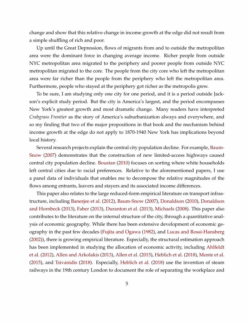
New York City was the largest city in the country at the beginning of the study period.Over the study period (1870-1940), the total population of the city increased from 1.48 mil-lion to 7.5 million.8 During the study period, the total population in NYC (5 boroughs)experienced an astonishing growth with its peak population growth rate being 39% overa decade. However, beginning in the early twentieth century, Manhattan experienced thedramatic population loss when all outer boroughs were gaining population at an unprece-dented rate (for example, between 1920 and 1930, Manhattan lost 18% of its populationwhen the population in Queens and Bronx grew by 130% and 73% respectively).
8In 1898, through the consolidation of NYC, outer boroughs (Brooklyn, Bronx, Queens, and Staten Island)were incorporated into New York City. For my analysis, I always define the city as 5 boroughs throughout thestudy period.
14
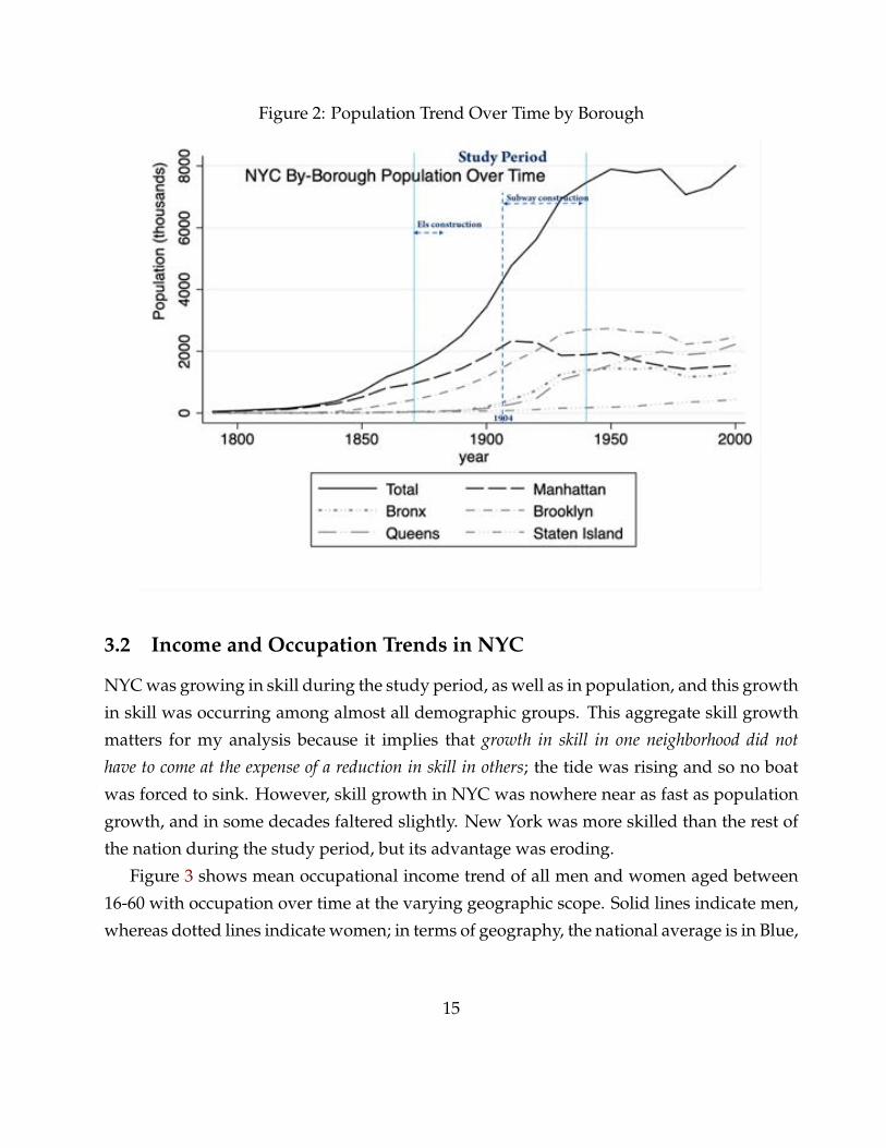
Figure 2: Population Trend Over Time by Borough
3.2 Income and Occupation Trends in NYC
NYC was growing in skill during the study period, as well as in population, and this growthin skill was occurring among almost all demographic groups. This aggregate skill growthmatters for my analysis because it implies that growth in skill in one neighborhood did nothave to come at the expense of a reduction in skill in others; the tide was rising and so no boatwas forced to sink. However, skill growth in NYC was nowhere near as fast as populationgrowth, and in some decades faltered slightly. New York was more skilled than the rest ofthe nation during the study period, but its advantage was eroding.
Figure 3 shows mean occupational income trend of all men and women aged between16-60 with occupation over time at the varying geographic scope. Solid lines indicate men,whereas dotted lines indicate women; in terms of geography, the national average is in Blue,
15

NYC’s metro area average is in Red9, and NYC average is in Green. Data reveal that men inNYC and NYC metro area had significantly higher mean occupational income than the restof the country, but converged to the rest of the country over the 60 years. A similar patternwas observed for women but at a much smaller magnitude.
Figure 3: Mean Occupational Income Trend: Men and Women
Source: US complete-count census records. All observations are aged between 16-60 with reportedoccupations.
9A metro area is a region consisting of a large urban core together with surrounding communities thathave a high degree of economic and social integration with the urban core. Since 1950, the Bureau of the Bud-get (later renamed the Office of Management and Budget, or OMB), has produced and continually updatedstandard delineations of metropolitan areas for the U.S. as a set of cities or towns. To delineate metro areasin pre-1950 samples (which is the case of all US census data that I use for the analysis), the general approach(used first by the creators of the 1940 PUMS and then by IPUMS for earlier samples) is to apply the 1950 OMBstandards to historical statistics. This approach of applying the 1950 OMB standards to pre-1950 samples hasmerits as it reflects the evolution of population and economic integration between surrounding areas and theurban core over time.
16

4 Testing the Specific Propositions of Crabgrass Frontier
4.1 Did Population Grow in More Suburban Areas?
As the distance from the center increases (measured by the distance from the Battery whichis the southern tip of Manhattan), the population density was declining during the studyperiod. Table 1 and Figure 4 show that the population density gradient was negative andflattening. With the NTAs (neighborhoods in the city) as the units of observation, I regresslog of population density as a function of the distance from the Battery to centroids of NTAsin the city. Regression results show that population gradient is negative and statisticallysignificant, but starting from the peak of subway construction in the 1910s, the populationdensity gradient was flattening significantly. The population density decreased as it getsfurther away from the center of the city. However, due to the transit infrastructure im-provement, the population grew in more suburban areas and therefore the density gradientwas flattening.10
The population grew in more suburban areas and Figure 7 shows this pattern over thestudy period. In 1880, only the center of the city and its adjacent areas were populated andareas further away from the center were largely unpopulated (“white shade” areas in Fig-ure 7 indicates unpopulated areas, whereas the darker shades of the color red, the higherpopulation density). However, starting from 1900, areas away from the center became pop-ulated and toward the end of the study period, in 1940, all neighborhoods in NYC becamepopulated. Similar patterns are observed in Figure 6: in the beginning of study period (in1880), only the areas close to the center were populated and areas further away from thecenter were largely unpopulated. Over time, areas relatively closer from the center becamepopulated, and the slope of bivariate plots became flatter which imply that the populationdensity declines less as the distance from the center increases. To the very end of studyperiod (in 1940), basically all areas in the city became populated.11
The population density in places close to the center (“transit-hub”) such as downtown
10This is consistent with the land use theory developed by Alonso (1964), Muth (1964), Mills (1967) whichpredicts that faster commuting times push up the demand for space in suburbs relative to central cities.
11In Figure 6, for ln (population density) (y-axis), I take the natural log of the total population in each NTAdivided by the size of each NTA. With regards to the distance from center (x-axis), I measure the distancefrom the Battery, the southern tip of Manhattan in NYC, to centroids of each NTA in the city (measured inkilometer). I assign the value of ln (population density) to be nil for unpopulated NTAs with population of 0.
17

and midtown Manhattan experienced dramatic losses, whereas “transit-spoke” neighbor-hoods such as upper Manhattan and Bronx, and Brooklyn were extensively gaining popu-lation.12 As in Figure 8, population density dramatically decreased in the center whereasthe population increased substantially in surrounding areas of the city center. During the1910s and 1920s, subway construction was at its peak through the Dual Contract period,and most neighborhoods in upper Manhattan, Brooklyn, and Bronx were experiencing ahuge improvement in commuting transit access.13
Table 1: Population Density (with zeros)
1870 1880 1900 1910 1920 1930 1940Dist Battery -0.0463*** -0.0984*** -0.0975*** -0.0898*** -0.0775*** -0.0467*** -0.0411***
(0.00831) (0.00831) (0.00883) (0.00852) (0.00853) (0.00614) (0.00609)Constant 3.167*** 6.488*** 8.260*** 8.794*** 8.736*** 8.456*** 8.348***
(0.417) (0.417) (0.443) (0.428) (0.428) (0.308) (0.306)N 195 195 195 195 195 195 195R2 0.139 0.421 0.387 0.365 0.300 0.230 0.191Standard errors in parentheses* p < 0.05, ** p < 0.01, *** p < 0.001
Note: Dependent variable: ln (population density) normalized by the size of each NTA (measured inkilometer2). Indepedent variable: distance from the Battery, the southern tip of Manhattan in NYC, to cen-troids of each NTA in the city (measured in kilometer). Here, when I take natural log of population density,I assign the value log(population density) to be nil for unpopulated NTAs with population of 0. 1870 (thefirst column) coefficient is less reliable as the availability of geographic information is extremely limited thatidentifying and harmonizing one’s residential location at NTA level was more challenging than other years.
12In the Appendix, I map the Transit Access changes by decade drive by the elevated and subway con-struction by every decade during the study period. At the same geographic and time scale, I also map thenew construction of residential-land use construction and commercial-land use construction by decade. Fig-ures show that in places near the center (“transit-hub”), land became more dedicated for commercial use;whereas places far from the center but connected to the center (“transit-spoke”), land became more dedicatedfor residential use.
13Finally, in the 1920s, subfigure 8d shows that the huge population decline in upper east Manhattan andHarlem during this period. Harlem was predominantly occupied by Jewish and Italian in the 19th century.However, in the 1920s and 1930s, during the Great Migration, African-American residents arrived in largenumbers and Harlem became the focus of the “Harlem Renaissance” and predominantly an African-Americancommunity.
18

Table 2: Population Density (without zeros)
1870 1880 1900 1910 1920 1930 1940Dist Battery -0.0691*** -0.0603*** -0.0630*** -0.0602*** -0.0569*** -0.0465*** -0.0361***
(0.0151) (0.00783) (0.00631) (0.00610) (0.00633) (0.00595) (0.00542)Constant 8.571*** 8.107*** 8.316*** 8.523*** 8.597*** 8.480*** 8.239***
(0.581) (0.264) (0.281) (0.284) (0.303) (0.299) (0.270)N 32 60 127 152 165 194 191R2 0.412 0.505 0.444 0.394 0.332 0.241 0.190Standard errors in parentheses* p < 0.05, ** p < 0.01, *** p < 0.001
Note: Dependent variable: ln (population density) normalized by the size of each NTA (measured inkilometer2). Indepedent variable: distance from the Battery, the southern tip of Manhattan in NYC, to cen-troids of each NTA in the city (measured in kilometer). Here, when I take natural log of population density,I excluded unpopulated NTAs with population of 0. 1870 (the first column) coefficient is less reliable as theavailability of geographic information is extremely limited that identifying and harmonizing one’s residentiallocation at NTA level was more challenging than other years.
19

Figure 4: Population Density Result Coefficients and Confidence Intervals (with zeros)
Note: When I take natural log of population density, I assign the value log(population density) to be nil forunpopulated NTAs with population of 0.
20

Figure 5: Population Density Result Coefficients and Confidence Intervals (without zeros)
-.1 -.08 -.06 -.04 -.02
1870 18801900 19101920 19301940
21
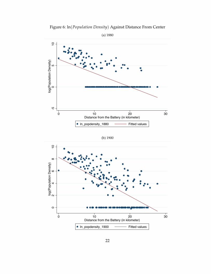
Figure 6: ln(Population Density) Against Distance From Center
(a) 1880
-50
510
log(
Popu
latio
n D
ensi
ty)
0 10 20 30Distance from the Battery (in kilometer)
ln_popdensity_1880 Fitted values
(b) 1900
02
46
810
log(
Popu
latio
n D
ensi
ty)
0 10 20 30Distance from the Battery (in kilometer)
ln_popdensity_1900 Fitted values
22
Figure 6: ln(Population Density) Against Distance From Center
(c) 1910
02
46
810
log(
Popu
latio
n D
ensi
ty)
0 10 20 30Distance from the Battery (in kilometer)
ln_popdensity_1910 Fitted values
(d) 1920
02
46
810
log(
Popu
latio
n D
ensi
ty)
0 10 20 30Distance from the Battery (in kilometer)
ln_popdensity_1920 Fitted values
23

Figure 6: ln(Population Density) Against Distance From Center
(e) 1930
-50
510
log(
Popu
latio
n D
ensi
ty)
0 10 20 30Distance from the Battery (in kilometer)
ln_popdensity_1930 Fitted values
(f) 1940
-50
510
log(
Popu
latio
n D
ensi
ty)
0 10 20 30Distance from the Battery (in kilometer)
ln_popdensity_1940 Fitted values
24
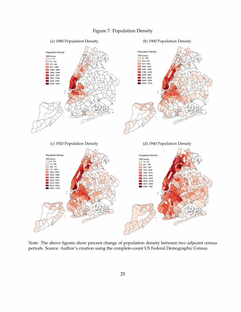
Figure 7: Population Density
(a) 1880 Population Density (b) 1900 Population Density
(c) 1920 Population Density (d) 1940 Population Density
Note: The above figures show percent change of population density between two adjacent censusperiods. Source: Author’s creation using the complete-count US Federal Demographic Census.
25

Figure 8: % Change of Population Density
(a) 1880-1900 Population Density % Change (b) 1900-10 Population Density % Change
(c) 1910-20 Population Density %Change (d) 1920-30 Population Density %Change
Note: The above figures show percent change of population density between two adjacent censusperiods. Source: Author’s Creation using the complete-count US Federal Demographic Census.
26

4.2 Did the Rich Leave the Center of the City?
Jackson (1985) discusses the phenomenon in the 1850s NYC of the rich leaving the center ofthe city. He discusses the migration of the rich in the center of the city by quoting phrasesconcerning the 1850s New York such as “the desertion of the city by its men of wealth” and“many of the rich and prosperous are removing from the city, while the poor are pressingin.”
If the popularly perceived pattern of the 1850s NYC had held true for my study period,the longitudinal database should reveal that leavers of the center of the city should be richerthan the stayers. Therefore, among residents of the center of the city, I compare the occu-pational income of residents who later moved (“leavers”) with that of those who stayed forthe next decade (“stayers”).
Throughout the period from 1880 to 1930, the longitudinal database shows that it wasnot the rich who left the center of the city. For example, Figures 9, 10, 11, 12 show that themean occupational income of city-center leavers was lower than that of city-center stayers.In each NTA, blue shades (the darker blue, the poorer leavers) indicate leavers being poorer,whereas red shades (the darker red, the richer leavers) indicate leavers being richer than thestayers. At the center of the city, throughout the years between 1880 and 1930, in Figures 9,10, 11, 12, the core of the city being consistently blue indicates that it was not the rich wholeft the center of the city—in fact, the leavers had lower mean occupational income than thecenter-stayers.
Regression results also show that it was not the rich who left the center of the city. Irun logistic regression (also called as a logit model) to model the log odds of individuals’leaving the city relative to staying in the city in the later period, using the longitudinal dataof individuals during the study period. The outcome of interest is identifying factors thatexplain whether individuals living in the core of the city in the early period leaves or staysthe city boundary (5 boroughs) in the subsequent period. The predictor variables of interestare occupational income, nativity, race, and age.
Regression results in Tables 3, 5, 7, 9, 11 show that as occupational income increases,people who lived in the city center in the earlier period were less likely to leave the city.In terms of the nativity, being foreign-born relative to native-born with both native parentsdecreases the log odds of leaving the city center — this may be partially due to ethnic
27
enclaves in Lower East Side of Manhattan near the city center. In terms of race, being non-white relative to white increases the log odds of leaving the city center and the degree ofrelative log odds across race differ; however, considering that the majority of residents inNew York were white, this may be interpreted with caution. Finally, older people are morelikely to leave throughout the study period.
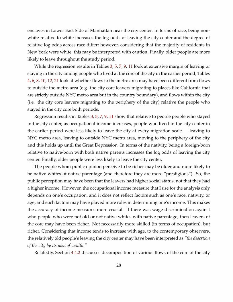
While the regression results in Tables 3, 5, 7, 9, 11 look at extensive margin of leaving orstaying in the city among people who lived at the core of the city in the earlier period, Tables4, 6, 8, 10, 12, 21 look at whether flows to the metro area may have been different from flowsto outside the metro area (e.g. the city core leavers migrating to places like California thatare strictly outside NYC metro area but in the country boundary), and flows within the city(i.e. the city core leavers migrating to the periphery of the city) relative the people whostayed in the city core both periods.
Regression results in Tables 3, 5, 7, 9, 11 show that relative to people people who stayedin the city center, as occupational income increases, people who lived in the city center inthe earlier period were less likely to leave the city at every migration scale — leaving toNYC metro area, leaving to outside NYC metro area, moving to the periphery of the cityand this holds up until the Great Depression. In terms of the nativity, being a foreign-bornrelative to native-born with both native parents increases the log odds of leaving the citycenter. Finally, older people were less likely to leave the city center.
The people whom public opinion perceive to be richer may be older and more likely tobe native whites of native parentage (and therefore they are more “prestigious”). So, thepublic perception may have been that the leavers had higher social status, not that they hada higher income. However, the occupational income measure that I use for the analysis onlydepends on one’s occupation, and it does not reflect factors such as one’s race, nativity, orage, and such factors may have played more roles in determining one’s income. This makesthe accuracy of income measures more crucial. If there was wage discrimination againstwho people who were not old or not native whites with native parentage, then leavers ofthe core may have been richer. Not necessarily more skilled (in terms of occupation), butricher. Considering that income tends to increase with age, to the contemporary observers,the relatively old people’s leaving the city center may have been interpreted as “the desertionof the city by its men of wealth.”
Relatedly, Section 4.4.2 discusses decomposition of various flows of the core of the city
28

including the relative income difference between leavers and stayers as well as the corre-sponding relative magnitudes of those flows at the neighborhood level. The people fromthe core who left the metropolitan area were richer than the people from the periphery wholeft the metropolitan area, and poorer people from outside NYC metro area migrated to thecore over time, making the relative income at the core to decrease.
Figure 9: Neighborhood-level Mean Income Differences between Leavers and Stayers, 1880-1900
Note: Blue shades mean leavers’ mean occupational income was lower than stayers, whereas red
shades mean leavers’ mean occupational income was higher than stayers in the Year 1880.
29

Table 3: Logit Results between Leavers and Stayers at the City level: 1880-1900 Males
[City Leavers]Occupational income -0.00517** -0.0101*** -0.0106*** -0.0121***
(0.00199) (0.00208) (0.00212) (0.00215)Nativity
Native born: both parents native - - -Native born: father foreign, mother native -1.350*** -1.357*** -1.295***
(0.205) (0.205) (0.206)Native born: mother foreign, father native -1.059*** -1.072*** -1.006***
(0.284) (0.285) (0.285)Native born: both parents foreign -1.488*** -1.501*** -1.422***
(0.0661) (0.0670) (0.0696)Foreign-born -0.177*** -0.191*** -0.206***
(0.0526) (0.0537) (0.0539)Race
White - -Black -0.229 -0.226
(0.180) (0.180)Chinese 0.156 0.218
(0.377) (0.378)Age 0.00979***
(0.00241)[City Stayers] (base outcome)N 9920 9920 9920 9920Standard errors in parentheses* p < 0.05, ** p < 0.01, *** p < 0.001
30
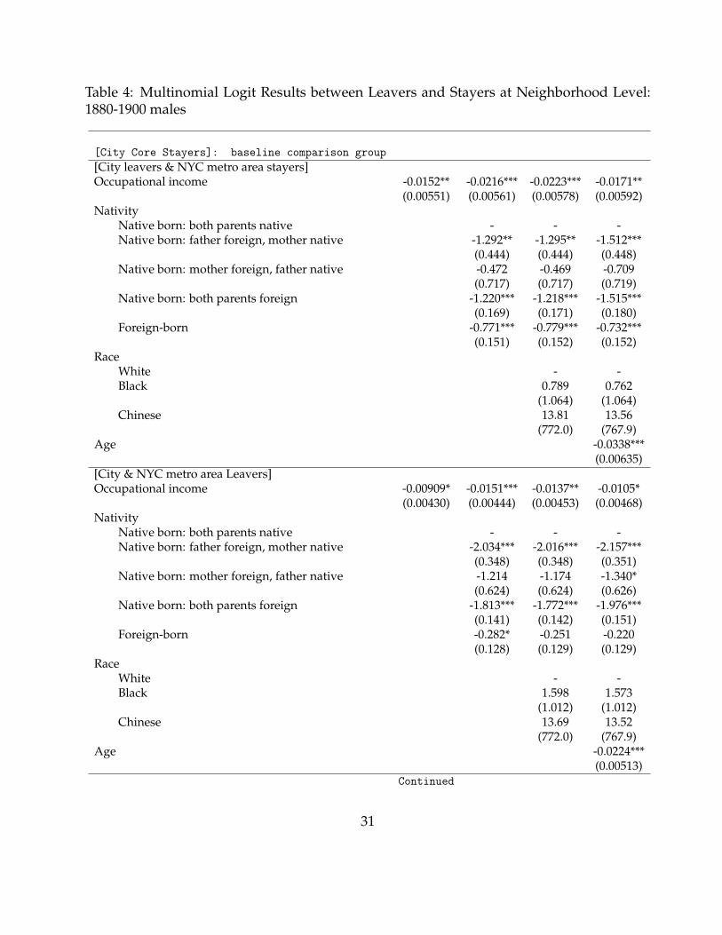
Table 4: Multinomial Logit Results between Leavers and Stayers at Neighborhood Level:1880-1900 males
[City Core Stayers]: baseline comparison group[City leavers & NYC metro area stayers]Occupational income -0.0152** -0.0216*** -0.0223*** -0.0171**
(0.00551) (0.00561) (0.00578) (0.00592)Nativity
Native born: both parents native - - -Native born: father foreign, mother native -1.292** -1.295** -1.512***
(0.444) (0.444) (0.448)Native born: mother foreign, father native -0.472 -0.469 -0.709
(0.717) (0.717) (0.719)Native born: both parents foreign -1.220*** -1.218*** -1.515***
(0.169) (0.171) (0.180)Foreign-born -0.771*** -0.779*** -0.732***
(0.151) (0.152) (0.152)Race
White - -Black 0.789 0.762
(1.064) (1.064)Chinese 13.81 13.56
(772.0) (767.9)Age -0.0338***
(0.00635)[City & NYC metro area Leavers]Occupational income -0.00909* -0.0151*** -0.0137** -0.0105*
(0.00430) (0.00444) (0.00453) (0.00468)Nativity
Native born: both parents native - - -Native born: father foreign, mother native -2.034*** -2.016*** -2.157***
(0.348) (0.348) (0.351)Native born: mother foreign, father native -1.214 -1.174 -1.340*
(0.624) (0.624) (0.626)Native born: both parents foreign -1.813*** -1.772*** -1.976***
(0.141) (0.142) (0.151)Foreign-born -0.282* -0.251 -0.220
(0.128) (0.129) (0.129)Race
White - -Black 1.598 1.573
(1.012) (1.012)Chinese 13.69 13.52
(772.0) (767.9)Age -0.0224***
(0.00513)Continued
31
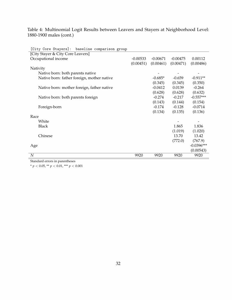
Table 4: Multinomial Logit Results between Leavers and Stayers at Neighborhood Level:1880-1900 males (cont.)
[City Core Stayers]: baseline comparison group[City Stayer & City Core Leavers]Occupational income -0.00533 -0.00671 -0.00475 0.00112
(0.00451) (0.00461) (0.00471) (0.00486)Nativity
Native born: both parents native - - -Native born: father foreign, mother native -0.685* -0.659 -0.911**
(0.345) (0.345) (0.350)Native born: mother foreign, father native -0.0412 0.0139 -0.264
(0.628) (0.628) (0.632)Native born: both parents foreign -0.274 -0.217 -0.557***
(0.143) (0.144) (0.154)Foreign-born -0.174 -0.128 -0.0714
(0.134) (0.135) (0.136)Race
White - -Black 1.865 1.836
(1.019) (1.020)Chinese 13.70 13.42
(772.0) (767.9)Age -0.0396***
(0.00543)N 9920 9920 9920 9920Standard errors in parentheses* p < 0.05, ** p < 0.01, *** p < 0.001
32
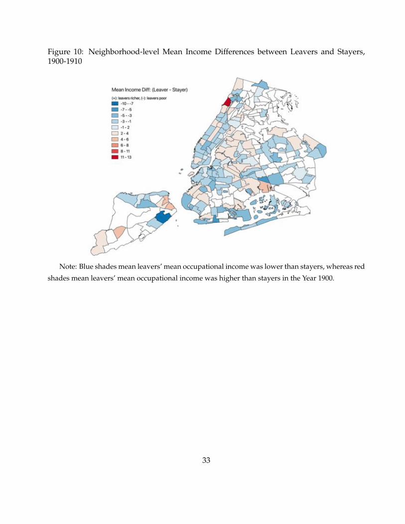
Figure 10: Neighborhood-level Mean Income Differences between Leavers and Stayers,1900-1910
Note: Blue shades mean leavers’ mean occupational income was lower than stayers, whereas red
shades mean leavers’ mean occupational income was higher than stayers in the Year 1900.
33

Table 5: Logit Results between Leavers and Stayers at the City level: 1900-1910 males
[City Leavers]Occupational income -0.0105*** -0.0103*** -0.00978*** -0.0112***
(0.00154) (0.00160) (0.00162) (0.00164)Nativity
Native born: both parents native - - -Native born: father foreign, mother native -1.377*** -1.373*** -1.318***
(0.145) (0.146) (0.146)Native born: mother foreign, father native -1.222*** -1.218*** -1.173***
(0.221) (0.221) (0.221)Native born: both parents foreign -1.003*** -1.000*** -0.981***
(0.0532) (0.0551) (0.0552)Foreign-born -0.343*** -0.350*** -0.371***
(0.0457) (0.0481) (0.0483)Race
White - -Black 0.0324 0.0228
(0.129) (0.129)Chinese 2.010*** 1.983***
(0.365) (0.366)Japanese 12.54 12.53
(526.8) (527.8)Age 0.0106***
(0.00148)[City Stayers] (base outcome)N 19085 19085 19085 19085Standard errors in parentheses* p < 0.05, ** p < 0.01, *** p < 0.001
34

Table 6: Multinomial Logit Results between Leavers and Stayers at Neighborhood Level:1900-1910 males
[City Core Stayers]: baseline comparison group[City leavers & NYC metro area stayers]Occupational income -0.0193*** -0.0197*** -0.0202*** -0.0171***
(0.00362) (0.00370) (0.00376) (0.00379)Nativity
Native born: both parents native - - -Native born: father foreign, mother native -0.802* -0.825* -0.956**
(0.321) (0.322) (0.323)Native born: mother foreign, father native -0.133 -0.159 -0.253
(0.458) (0.459) (0.461)Native born: both parents foreign -0.209 -0.235 -0.284*
(0.128) (0.132) (0.133)Foreign-born -0.140 -0.171 -0.123
(0.109) (0.114) (0.114)Race
White - -Black -0.252 -0.236
(0.314) (0.314)Chinese 13.60 13.90
(483.6) (548.2)Japanese -0.0292 -0.0355
(6027.3) (6776.7)Age -0.0244***
(0.00369)[City & NYC metro area Leavers]Occupational income -0.0262*** -0.0252*** -0.0249*** -0.0238***
(0.00256) (0.00263) (0.00267) (0.00269)Nativity
Native born: both parents native - - -Native born: father foreign, mother native -1.455*** -1.459*** -1.511***
(0.226) (0.227) (0.227)Native born: mother foreign, father native -1.230** -1.234** -1.265***
(0.375) (0.376) (0.377)Native born: both parents foreign -0.627*** -0.632*** -0.655***
(0.0981) (0.101) (0.102)Foreign-born -0.114 -0.132 -0.116
(0.0834) (0.0874) (0.0876)Race
White - -Black -0.0562 -0.0552
(0.237) (0.237)Chinese 14.80 15.07
(483.6) (548.2)Japanese 15.22 15.45
(4208.0) (4690.4)Age -0.00908***
(0.00271)Continued
35

Table 6: Multinomial Logit Results between Leavers and Stayers at Neighborhood Level:1900-1910 males (cont.)
[City Core Stayers]: baseline comparison group[City Stayer & City Core Leavers]Occupational income -0.0193*** -0.0188*** -0.0191*** -0.0157***
(0.00271) (0.00281) (0.00285) (0.00288)Nativity
Native born: both parents native - - -Native born: father foreign, mother native 0.0217 0.0101 -0.134
(0.221) (0.222) (0.223)Native born: mother foreign, father native 0.239 0.226 0.122
(0.366) (0.367) (0.370)Native born: both parents foreign 0.541*** 0.528*** 0.475***
(0.104) (0.108) (0.108)Foreign-born 0.295** 0.279** 0.332***
(0.0911) (0.0954) (0.0958)Race
White - -Black -0.133 -0.114
(0.260) (0.261)Chinese 12.91 13.22
(483.6) (548.2)Japanese -0.0173 -0.0185
(4729.7) (5291.0)Age -0.0271***
(0.00290)N 19100 19100 19100 19100Standard errors in parentheses* p < 0.05, ** p < 0.01, *** p < 0.001
36

Figure 11: Neighborhood-level Mean Income Differences between Leavers and Stayers,1910-1920
Note: Blue shades mean leavers’ mean occupational income was lower than stayers, whereas red
shades mean leavers’ mean occupational income was higher than stayers in the Year 1910.
37
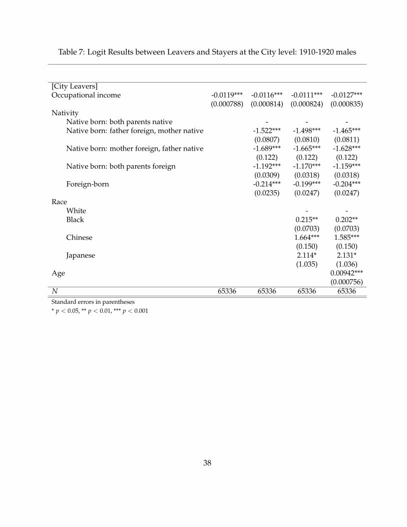
Table 7: Logit Results between Leavers and Stayers at the City level: 1910-1920 males
[City Leavers]Occupational income -0.0119*** -0.0116*** -0.0111*** -0.0127***
(0.000788) (0.000814) (0.000824) (0.000835)Nativity
Native born: both parents native - - -Native born: father foreign, mother native -1.522*** -1.498*** -1.465***
(0.0807) (0.0810) (0.0811)Native born: mother foreign, father native -1.689*** -1.665*** -1.628***
(0.122) (0.122) (0.122)Native born: both parents foreign -1.192*** -1.170*** -1.159***
(0.0309) (0.0318) (0.0318)Foreign-born -0.214*** -0.199*** -0.204***
(0.0235) (0.0247) (0.0247)Race
White - -Black 0.215** 0.202**
(0.0703) (0.0703)Chinese 1.664*** 1.585***
(0.150) (0.150)Japanese 2.114* 2.131*
(1.035) (1.036)Age 0.00942***
(0.000756)N 65336 65336 65336 65336Standard errors in parentheses* p < 0.05, ** p < 0.01, *** p < 0.001
38

Table 8: Multinomial Logit Results between Leavers and Stayers at Neighborhood Level:1910-1920 males
[City Core Stayers]: baseline comparison group[City leavers & NYC metro area stayers]Occupational income -0.0169*** -0.0161*** -0.0171*** -0.0132***
(0.00182) (0.00186) (0.00189) (0.00191)Nativity
Native born: both parents native - - -Native born: father foreign, mother native -0.821*** -0.873*** -0.954***
(0.152) (0.152) (0.153)Native born: mother foreign, father native -1.008*** -1.060*** -1.147***
(0.230) (0.231) (0.231)Native born: both parents foreign -0.509*** -0.564*** -0.585***
(0.0668) (0.0682) (0.0683)Foreign-born 0.0225 -0.0318 -0.0188
(0.0550) (0.0568) (0.0569)Race
White - -Black -0.747*** -0.722***
(0.206) (0.206)Chinese -0.854* -0.686
(0.416) (0.417)Japanese -0.343 -0.403
(1406.6) (1404.9)Age -0.0221***
(0.00179)[City & NYC metro area Leavers]Occupational income -0.0240*** -0.0216*** -0.0207*** -0.0182***
(0.00126) (0.00131) (0.00132) (0.00134)Nativity
Native born: both parents native - - -Native born: father foreign, mother native -1.868*** -1.827*** -1.878***
(0.114) (0.115) (0.115)Native born: mother foreign, father native -2.007*** -1.967*** -2.020***
(0.169) (0.169) (0.170)Native born: both parents foreign -1.282*** -1.242*** -1.255***
(0.0494) (0.0508) (0.0509)Foreign-born 0.116** 0.150*** 0.157***
(0.0406) (0.0423) (0.0424)Race
White - -Black 0.328* 0.342**
(0.127) (0.128)Chinese 1.008*** 1.107***
(0.226) (0.226)Japanese 14.14 14.09
(933.6) (930.9)Age -0.0138***
(0.00128)Continued
39
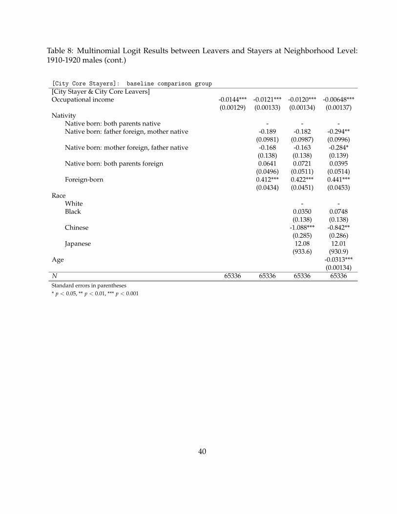
Table 8: Multinomial Logit Results between Leavers and Stayers at Neighborhood Level:1910-1920 males (cont.)
[City Core Stayers]: baseline comparison group[City Stayer & City Core Leavers]Occupational income -0.0144*** -0.0121*** -0.0120*** -0.00648***
(0.00129) (0.00133) (0.00134) (0.00137)Nativity
Native born: both parents native - - -Native born: father foreign, mother native -0.189 -0.182 -0.294**
(0.0981) (0.0987) (0.0996)Native born: mother foreign, father native -0.168 -0.163 -0.284*
(0.138) (0.138) (0.139)Native born: both parents foreign 0.0641 0.0721 0.0395
(0.0496) (0.0511) (0.0514)Foreign-born 0.412*** 0.422*** 0.441***
(0.0434) (0.0451) (0.0453)Race
White - -Black 0.0350 0.0748
(0.138) (0.138)Chinese -1.088*** -0.842**
(0.285) (0.286)Japanese 12.08 12.01
(933.6) (930.9)Age -0.0313***
(0.00134)N 65336 65336 65336 65336Standard errors in parentheses* p < 0.05, ** p < 0.01, *** p < 0.001
40

Figure 12: Neighborhood-level Mean Income Differences between Leavers and Stayers,1920-1930
Note: Blue shades mean leavers’ mean occupational income was lower than stayers, whereas red
shades mean leavers’ mean occupational income was higher than stayers in the Year 1920.
41
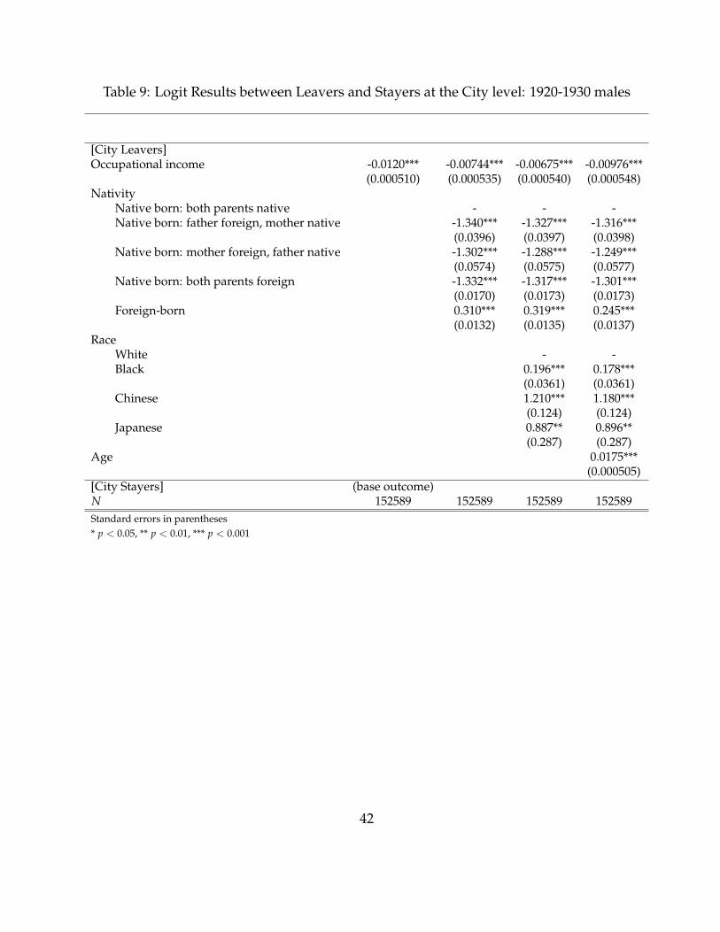
Table 9: Logit Results between Leavers and Stayers at the City level: 1920-1930 males
[City Leavers]Occupational income -0.0120*** -0.00744*** -0.00675*** -0.00976***
(0.000510) (0.000535) (0.000540) (0.000548)Nativity
Native born: both parents native - - -Native born: father foreign, mother native -1.340*** -1.327*** -1.316***
(0.0396) (0.0397) (0.0398)Native born: mother foreign, father native -1.302*** -1.288*** -1.249***
(0.0574) (0.0575) (0.0577)Native born: both parents foreign -1.332*** -1.317*** -1.301***
(0.0170) (0.0173) (0.0173)Foreign-born 0.310*** 0.319*** 0.245***
(0.0132) (0.0135) (0.0137)Race
White - -Black 0.196*** 0.178***
(0.0361) (0.0361)Chinese 1.210*** 1.180***
(0.124) (0.124)Japanese 0.887** 0.896**
(0.287) (0.287)Age 0.0175***
(0.000505)[City Stayers] (base outcome)N 152589 152589 152589 152589Standard errors in parentheses* p < 0.05, ** p < 0.01, *** p < 0.001
42

Table 10: Multinomial Logit Results between Leavers and Stayers at Neighborhood Level:1920-1930 males
[City Core Stayers]: baseline comparison group[City leavers & NYC metro area stayers]Occupational income -0.0129*** -0.00998*** -0.0116*** -0.00765***
(0.00108) (0.00110) (0.00112) (0.00114)Nativity
Native born: both parents native - - -Native born: father foreign, mother native -0.765*** -0.827*** -0.842***
(0.0676) (0.0678) (0.0679)Native born: mother foreign, father native -0.685*** -0.750*** -0.794***
(0.0972) (0.0974) (0.0976)Native born: both parents foreign -0.672*** -0.740*** -0.752***
(0.0346) (0.0350) (0.0351)Foreign-born 0.331*** 0.273*** 0.359***
(0.0308) (0.0312) (0.0317)Race
White - -Black -1.175*** -1.152***
(0.106) (0.106)Chinese -0.874** -0.843**
(0.271) (0.271)Japanese -1.531 -1.552
(1.118) (1.118)Age -0.0206***
(0.00110)[City & NYC metro area Leavers]Occupational income -0.0244*** -0.0182*** -0.0179*** -0.0163***
(0.000785) (0.000817) (0.000823) (0.000837)Nativity
Native born: both parents native - - -Native born: father foreign, mother native -1.842*** -1.845*** -1.848***
(0.0570) (0.0572) (0.0572)Native born: mother foreign, father native -1.785*** -1.788*** -1.796***
(0.0832) (0.0833) (0.0834)Native born: both parents foreign -1.450*** -1.453*** -1.452***
(0.0263) (0.0268) (0.0269)Foreign-born 0.548*** 0.544*** 0.566***
(0.0231) (0.0235) (0.0238)Race
White - -Black -0.0784 -0.0626
(0.0566) (0.0567)Chinese 0.124 0.140
(0.164) (0.164)Japanese 0.569 0.565
(0.521) (0.520)Age -0.00523***
(0.000799)Continued43
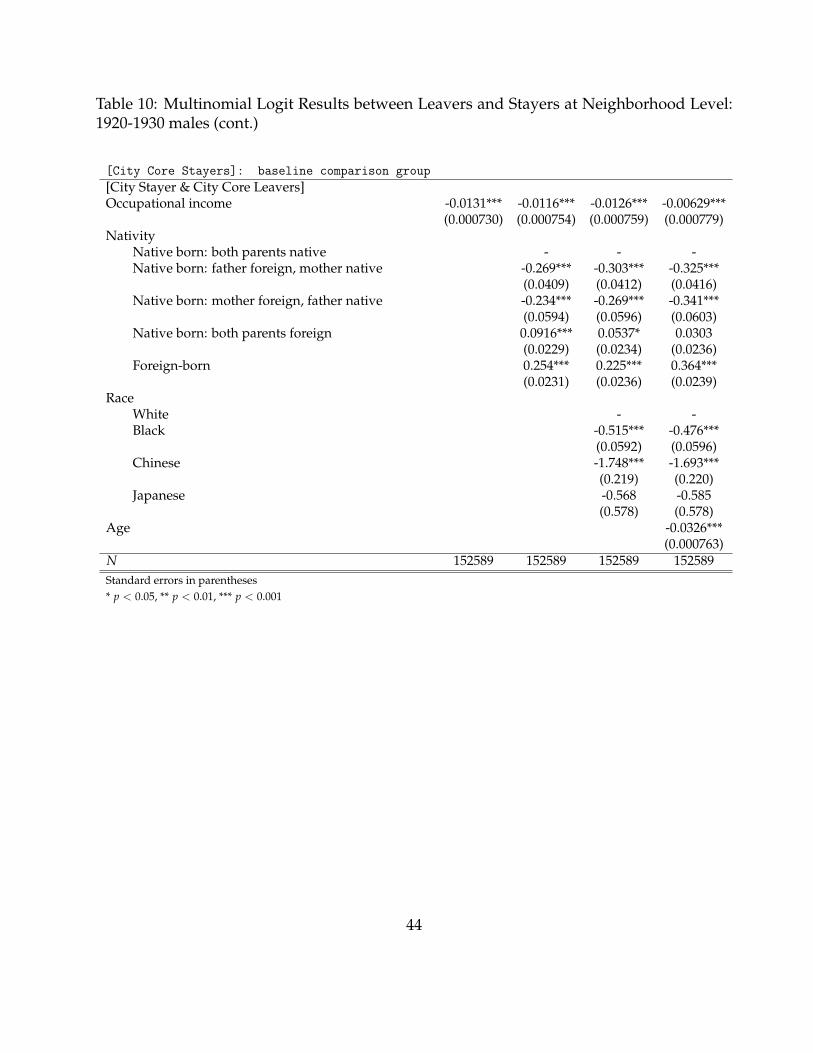
Table 10: Multinomial Logit Results between Leavers and Stayers at Neighborhood Level:1920-1930 males (cont.)
[City Core Stayers]: baseline comparison group[City Stayer & City Core Leavers]Occupational income -0.0131*** -0.0116*** -0.0126*** -0.00629***
(0.000730) (0.000754) (0.000759) (0.000779)Nativity
Native born: both parents native - - -Native born: father foreign, mother native -0.269*** -0.303*** -0.325***
(0.0409) (0.0412) (0.0416)Native born: mother foreign, father native -0.234*** -0.269*** -0.341***
(0.0594) (0.0596) (0.0603)Native born: both parents foreign 0.0916*** 0.0537* 0.0303
(0.0229) (0.0234) (0.0236)Foreign-born 0.254*** 0.225*** 0.364***
(0.0231) (0.0236) (0.0239)Race
White - -Black -0.515*** -0.476***
(0.0592) (0.0596)Chinese -1.748*** -1.693***
(0.219) (0.220)Japanese -0.568 -0.585
(0.578) (0.578)Age -0.0326***
(0.000763)N 152589 152589 152589 152589Standard errors in parentheses* p < 0.05, ** p < 0.01, *** p < 0.001
44
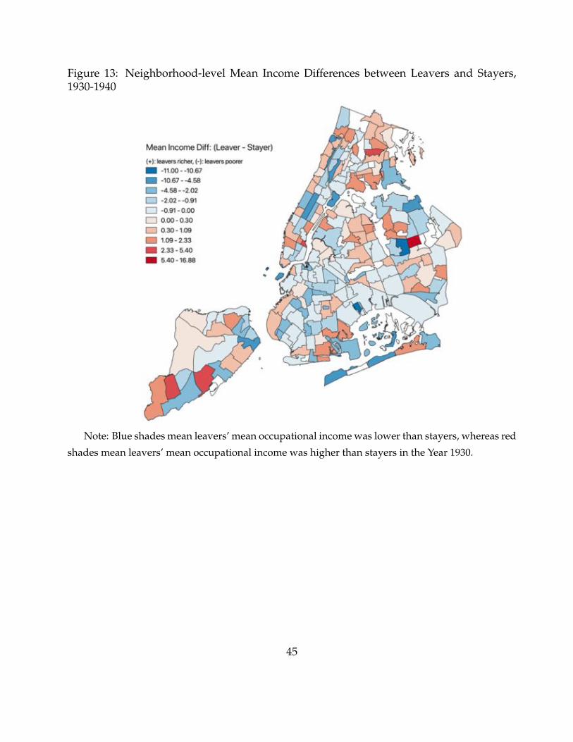
Figure 13: Neighborhood-level Mean Income Differences between Leavers and Stayers,1930-1940
Note: Blue shades mean leavers’ mean occupational income was lower than stayers, whereas red
shades mean leavers’ mean occupational income was higher than stayers in the Year 1930.
45

Table 11: Logit Results between Leavers and Stayers at the City level: 1930-1940 males
[City Leavers]Occupational income 0.00198 -0.00555** -0.00471* -0.00676**
(0.00194) (0.00206) (0.00209) (0.00213)Nativity
Native born: both parents native - - -Native born: father foreign, mother native -0.744*** -0.767*** -0.761***
(0.129) (0.129) (0.129)Native born: mother foreign, father native -0.385* -0.400** -0.384*
(0.152) (0.152) (0.152)Native born: both parents foreign -1.264*** -1.272*** -1.220***
(0.0634) (0.0642) (0.0649)Foreign-born -0.681*** -0.722*** -0.778***
(0.0555) (0.0566) (0.0578)Race
White - -Black -0.203 -0.227
(0.177) (0.178)Chinese 0.751*** 0.744***
(0.158) (0.158)Japanese 0.935 0.836
(0.867) (0.868)Age 0.0113***
(0.00211)[City Stayers] (base outcome)N 8789 8789 8789 8789Standard errors in parentheses* p < 0.05, ** p < 0.01, *** p < 0.001
46

Table 12: Multinomial Logit Results between Leavers and Stayers at Neighborhood Level:1930-1940 males
[City Core Stayers]: baseline comparison group[City leavers & NYC metro area stayers]Occupational income 0.00650 -0.00143 -0.00366 0.000959
(0.00388) (0.00405) (0.00410) (0.00419)Nativity
Native born: both parents native - - -Native born: father foreign, mother native -0.551* -0.551* -0.557*
(0.258) (0.259) (0.260)Native born: mother foreign, father native 0.108 0.102 0.0665
(0.308) (0.308) (0.309)Native born: both parents foreign -0.743*** -0.762*** -0.878***
(0.128) (0.129) (0.131)Foreign-born -0.964*** -0.924*** -0.803***
(0.121) (0.122) (0.124)Race
White - -Black -0.391 -0.339
(0.465) (0.466)Chinese -1.594*** -1.590***
(0.475) (0.475)Japanese -13.46 -12.95
(1221.9) (1047.5)Age -0.0251***
(0.00439)[City & NYC metro area Leavers]Occupational income -0.00398 -0.0130*** -0.0130*** -0.0110***
(0.00295) (0.00307) (0.00308) (0.00314)Nativity
Native born: both parents native - - -Native born: father foreign, mother native -0.903*** -0.907*** -0.905***
(0.199) (0.199) (0.200)Native born: mother foreign, father native -0.439 -0.433 -0.449
(0.260) (0.260) (0.260)Native born: both parents foreign -1.435*** -1.429*** -1.480***
(0.101) (0.102) (0.104)Foreign-born -0.874*** -0.865*** -0.815***
(0.0899) (0.0918) (0.0932)Race
White - -Black 0.136 0.156
(0.322) (0.323)Chinese -0.152 -0.154
(0.179) (0.179)Japanese 0.461 0.546
(1.122) (1.123)Age -0.0109***
(0.00312)Continued
47

Table 12: Multinomial Logit Results between Leavers and Stayers at Neighborhood Level:1930-1940 males (cont.)
[City Core Stayers]: baseline comparison group[City Stayer & City Core Leavers]Occupational income -0.00516 -0.00680* -0.00875** -0.00242
(0.00291) (0.00296) (0.00298) (0.00306)Nativity
Native born: both parents native - - -Native born: father foreign, mother native -0.114 -0.0854 -0.0989
(0.192) (0.193) (0.195)Native born: mother foreign, father native 0.0877 0.115 0.0679
(0.260) (0.260) (0.262)Native born: both parents foreign -0.0144 -0.00155 -0.163
(0.0978) (0.0990) (0.101)Foreign-born -0.281** -0.206* -0.0365
(0.0924) (0.0940) (0.0959)Race
White - -Black 0.335 0.408
(0.326) (0.328)Chinese -2.080*** -2.070***
(0.279) (0.280)Japanese -1.029 -0.730
(1.416) (1.419)Age -0.0350***
(0.00312)N 8789 8789 8789 8789Standard errors in parentheses* p < 0.05, ** p < 0.01, *** p < 0.001
4.3 Were the People Who Moved Into the Periphery Richer than Original
Residents of the Periphery?
Jackson (1985) discusses Brooklyn’s transformation from being essentially agricultural tothe favorite residence of gentlemen of taste and fortune between the 1810s and the 1850s dueto the regular steam ferry service to the NYC. During the early nineteenth century, Brooklynbecame the “transit-hub” connected to the center of the city, and the influx of middle-classfamilies changed the orientation of neighborhoods — “the little village of Bedford (nowpart of Bedford-Stuyvesant in Northeast Brooklyn), for example, used to be essentially rural
48

until 1850. However, after the influx of middle-class families, and it had become part of theexpanding metropolis, very few laborers remained, and the farmers had disappeared.”14
If the pattern of early nineteenth-century Brooklyn as the periphery of the city as thetransit spoke held for my study period, the longitudinal database should reveal that en-trants who moved into the periphery were richer than original residents of the periphery ofthe city. Hence, I take the longitudinal data of individuals and compare the mean occupa-tional income of residents who moved into the periphery and who stayed in the peripheryat the NTA level.
The longitudinal data reveals that the entrants who moved into the periphery were notricher than the original residents of the periphery. For example, Figures 15, 16, 17 show thatthe entrants to the periphery had mostly lower mean occupational income than the originalresidents. Given each NTA in the City, I take the difference of mean occupational income ofentrants and stayers at the periphery over the study period. In Figures 14, 15, 16, 17, giveneach NTA, blue shades (the darker blue, the poorer entrants) indicate entrants being poorer,whereas red shades (the darker red, the richer entrants) indicate entrants being richer thanthe stayers. Data during the study period indicates that the entrants to the periphery were,in fact, not richer than the stayers.
Regression results also support that new suburbanites were not richer than the peoplewho already lived at the periphery. I run logit regression to model the log odds of indi-viduals’ entering into the city periphery, using the longitudinal data of individuals duringthe study period. The predictor variables of interest are occupational income, nativity, race,and age. Regression results in Tables 13, 15, 17, 19 show that as one’s occupational incomeincreases, the log odds of moving into the city periphery decreases. In terms of the na-tivity, being foreign-born relative to native-born with both native parents (which may beassociated with one’s “prestige to the public’s eye) decreases the log odds of entering thecity periphery. In terms of race, being non-white relative to white increases the log odds ofmoving into the periphery and the degree of log odds of outcome varies across race; how-ever, considering that the majority of residents in New York were white, this may need tobe interpreted with caution. Finally, older people were more likely to enter into the cityperiphery throughout the study period.
While the regression results in Tables 13, 15, 17, 19 look at extensive margin of entering14Recited from Jackson (1985), originally from Gilman (1971).
49

to the periphery of the city regardless of the nature of flows (i.e. whether entrants migratedto the city’s periphery from NYC metro area, or migrated from Alabama, or migrated fromthe core of the city), Tables 14, 16, 18, 20, 22 look at whether flows from the metro area tothe city periphery may have been different from flows from outside the metro area to thecity periphery, as well as flows from the city core to the city periphery. Regression resultsregarding city periphery entrants that separately looks at entrants with varying origins tellsus consistent story (as in periphery entrants at the extensive margin regardless of origins)that relative to people who stayed in the city periphery, as occupational income increases,people who lived somewhere other than the city periphery (at any migration origins rang-ing from the city core to outside NYC metro area) were less likely to migrate to the cityperiphery. In terms of race, being non-white relative to white has varying degree and signsdepending on origins of migration, however, considering that the majority of residents inNew York were white, this may need to be interpreted with caution. Finally, older peoplewere less likely to migrate into the city periphery up until the Great Depression.
Related to my earlier discussion of income measures feature of reflecting occupationonly and not reflecting other factors such as nativity and age that may have determinedone’s income should be noted in interpreting suburbanites’ pattern of migration.15 To thepublic’s eyes, migration of the older to the periphery may have been associated as the move-ment of the “affluent.” However, this only makes the accuracy of income measures morecrucial.
Section 4.4.2 discusses decomposition of various flows of the periphery of the city in-cluding the relative income difference between entrants and stayers as well as the corre-sponding relative magnitudes of those flows at the neighborhood level. Regarding the rela-tive income growth at the periphery, periphery entrants from anywhere (from the city core,NYC metro area, and outside NYC metro area) had higher mean income than the peripheryleaving NYC metro area at all, and the relative magnitude of inflows were much biggerthan outflows, making the periphery income increase. Furthermore, as Figure 22b shows,people who stayed at the periphery got richer as the metropolis grew.
15Features of occupational income measures are discussed in Subsection 4.2.
50
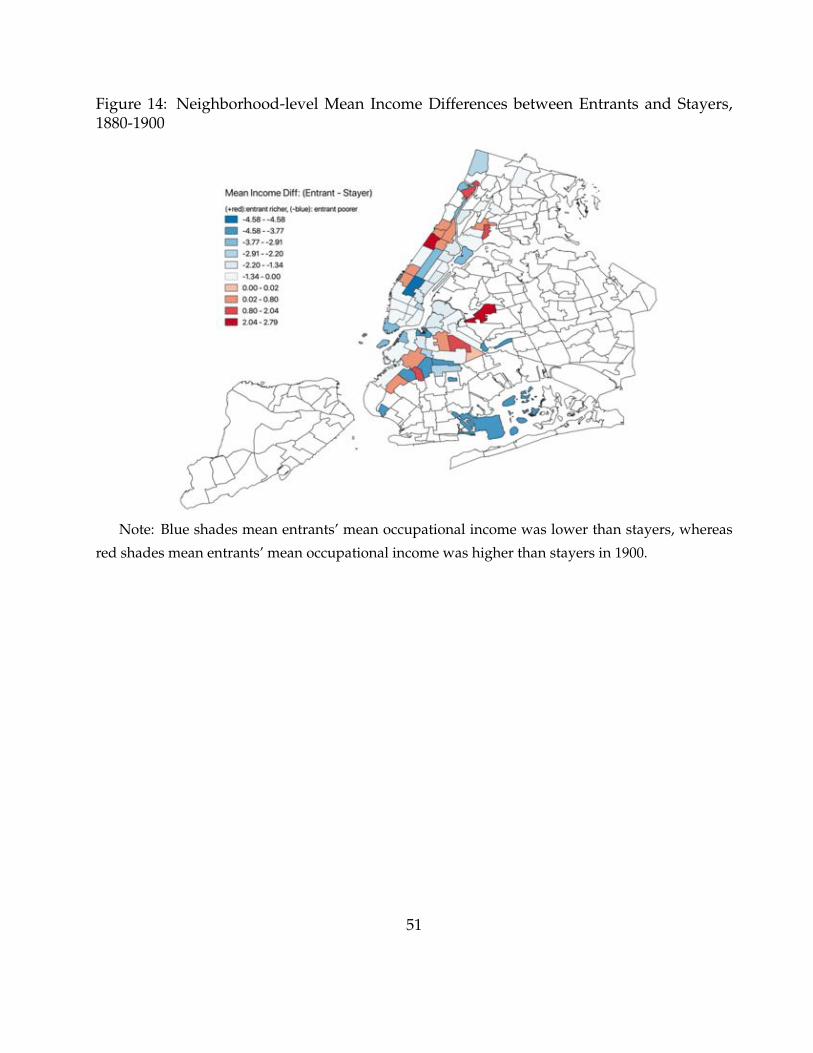
Figure 14: Neighborhood-level Mean Income Differences between Entrants and Stayers,1880-1900
Note: Blue shades mean entrants’ mean occupational income was lower than stayers, whereas
red shades mean entrants’ mean occupational income was higher than stayers in 1900.
51

Table 13: Logit Results between Entrants and Stayers at the City level: 1880-1900 males
[City Entrants]Occupational income -0.00169 -0.00674*** -0.00538** -0.00554**
(0.00160) (0.00171) (0.00174) (0.00175)Nativity
Native born: both parents native - - -Native born: father foreign, mother native -1.529*** -1.514*** -1.548***
(0.153) (0.153) (0.153)Native born: mother foreign, father native -1.125*** -1.119*** -1.133***
(0.221) (0.221) (0.221)Native born: both parents foreign -1.832*** -1.812*** -1.899***
(0.0542) (0.0546) (0.0563)Foreign-born -0.650*** -0.645*** -0.603***
(0.0425) (0.0432) (0.0436)Race
White - -Black 0.390* 0.330*
(0.154) (0.154)Chinese 2.578*** 2.484***
(0.594) (0.594)Age -0.0134***
(0.00196)[City Stayers] (base outcome)N 13239 13239 13239 13239Standard errors in parentheses* p < 0.05, ** p < 0.01, *** p < 0.001
52
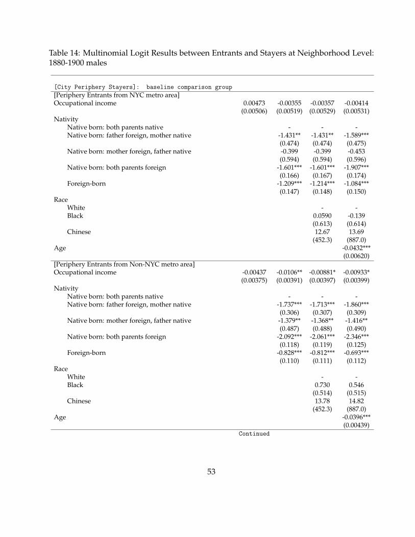
Table 14: Multinomial Logit Results between Entrants and Stayers at Neighborhood Level:1880-1900 males
[City Periphery Stayers]: baseline comparison group[Periphery Entrants from NYC metro area]Occupational income 0.00473 -0.00355 -0.00357 -0.00414
(0.00506) (0.00519) (0.00529) (0.00531)Nativity
Native born: both parents native - - -Native born: father foreign, mother native -1.431** -1.431** -1.589***
(0.474) (0.474) (0.475)Native born: mother foreign, father native -0.399 -0.399 -0.453
(0.594) (0.594) (0.596)Native born: both parents foreign -1.601*** -1.601*** -1.907***
(0.166) (0.167) (0.174)Foreign-born -1.209*** -1.214*** -1.084***
(0.147) (0.148) (0.150)Race
White - -Black 0.0590 -0.139
(0.613) (0.614)Chinese 12.67 13.69
(452.3) (887.0)Age -0.0432***
(0.00620)[Periphery Entrants from Non-NYC metro area]Occupational income -0.00437 -0.0106** -0.00881* -0.00933*
(0.00375) (0.00391) (0.00397) (0.00399)Nativity
Native born: both parents native - - -Native born: father foreign, mother native -1.737*** -1.713*** -1.860***
(0.306) (0.307) (0.309)Native born: mother foreign, father native -1.379** -1.368** -1.416**
(0.487) (0.488) (0.490)Native born: both parents foreign -2.092*** -2.061*** -2.346***
(0.118) (0.119) (0.125)Foreign-born -0.828*** -0.812*** -0.693***
(0.110) (0.111) (0.112)Race
White - -Black 0.730 0.546
(0.514) (0.515)Chinese 13.78 14.82
(452.3) (887.0)Age -0.0396***
(0.00439)Continued
53

Table 14: Multinomial Logit Results between Entrants and Stayers at Neighborhood Level:1880-1900 males (cont.)
[City Periphery Stayers]: baseline comparison group[Periphery Entrants from the City’s Core]Occupational income -0.00226 -0.00367 -0.00340 -0.00379
(0.00383) (0.00395) (0.00401) (0.00402)Nativity
Native born: both parents native - - -Native born: father foreign, mother native -0.205 -0.196 -0.313
(0.298) (0.298) (0.299)Native born: mother foreign, father native -0.154 -0.149 -0.188
(0.483) (0.483) (0.484)Native born: both parents foreign -0.242* -0.232* -0.457***
(0.117) (0.118) (0.123)Foreign-born -0.225* -0.215 -0.126
(0.113) (0.114) (0.115)Race
White - -Black 0.331 0.189
(0.528) (0.529)Chinese 11.29 12.40
(452.3) (887.0)Age -0.0299***
(0.00446)N 13239 13239 13239 13239Standard errors in parentheses* p < 0.05, ** p < 0.01, *** p < 0.001
54

Figure 15: Neighborhood-level Mean Income Differences between Entrants and Stayers,1900-1910
Note: Blue shades mean entrants’ mean occupational income was lower than stayers, whereas
red shades mean entrants’ mean occupational income was higher than stayers in 1910.
55

Table 15: Logit Results between Entrants and Stayers: 1900-1910 males
[City Entrants]Occupational income -0.00774*** -0.00671*** -0.00608*** -0.00671***
(0.000945) (0.000986) (0.000998) (0.00100)Nativity
Native born: both parents native - - -Native born: father foreign, mother native -1.354*** -1.328*** -1.272***
(0.0710) (0.0713) (0.0716)Native born: mother foreign, father native -1.207*** -1.181*** -1.148***
(0.114) (0.114) (0.114)Native born: both parents foreign -1.189*** -1.161*** -1.162***
(0.0330) (0.0338) (0.0338)Foreign-born -0.143*** -0.117*** -0.170***
(0.0287) (0.0297) (0.0301)Race
White - -Black 0.331*** 0.367***
(0.0940) (0.0941)Chinese 1.360** 1.365**
(0.427) (0.428)Japanese 14.06 14.12
(1265.8) (1265.7)Age 0.0118***
(0.00101)[City Stayers] (base outcome)N 47201 47201 47201 47201Standard errors in parentheses* p < 0.05, ** p < 0.01, *** p < 0.001
56

Table 16: Multinomial Logit Results between Entrants and Stayers at Neighborhood Level:1900-1910 males
[City Periphery Stayers]: baseline comparison group[Periphery Entrants from NYC metro area]Occupational income -0.0121*** -0.0109*** -0.0112*** -0.0100***
(0.00256) (0.00261) (0.00265) (0.00266)Nativity
Native born: both parents native - - -Native born: father foreign, mother native -1.019*** -1.025*** -1.144***
(0.173) (0.174) (0.175)Native born: mother foreign, father native -1.149*** -1.156*** -1.227***
(0.294) (0.295) (0.295)Native born: both parents foreign -0.463*** -0.471*** -0.479***
(0.0848) (0.0863) (0.0864)Foreign-born 0.0536 0.0453 0.144
(0.0760) (0.0778) (0.0787)Race
White - -Black -0.0542 -0.136
(0.278) (0.278)Chinese 0.339 0.310
(1.226) (1.226)Japanese -0.430 -0.584
(2134.9) (3520.6)Age -0.0224***
(0.00266)[Periphery Entrants from Non-NYC metro area]Occupational income -0.0145*** -0.0118*** -0.0108*** -0.0100***
(0.00186) (0.00191) (0.00194) (0.00195)Nativity
Native born: both parents native - - -Native born: father foreign, mother native -1.616*** -1.574*** -1.658***
(0.115) (0.115) (0.116)Native born: mother foreign, father native -1.474*** -1.431*** -1.481***
(0.181) (0.181) (0.181)Native born: both parents foreign -1.048*** -1.002*** -1.011***
(0.0638) (0.0650) (0.0651)Foreign-born 0.181** 0.225*** 0.292***
(0.0589) (0.0603) (0.0609)Race
White - -Black 0.609** 0.550*
(0.214) (0.215)Chinese 1.327 1.298
(1.009) (1.009)Japanese 12.58 13.47
(1555.1) (2564.6)Age -0.0154***
(0.00199)Continued
57
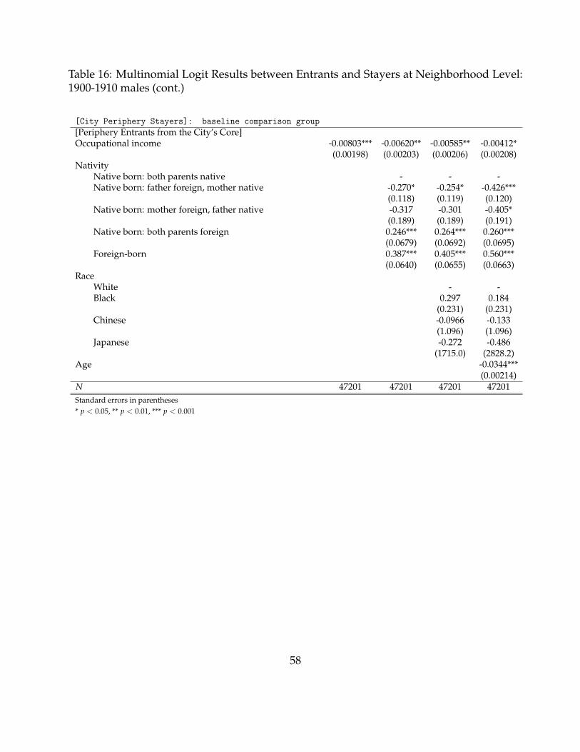
Table 16: Multinomial Logit Results between Entrants and Stayers at Neighborhood Level:1900-1910 males (cont.)
[City Periphery Stayers]: baseline comparison group[Periphery Entrants from the City’s Core]Occupational income -0.00803*** -0.00620** -0.00585** -0.00412*
(0.00198) (0.00203) (0.00206) (0.00208)Nativity
Native born: both parents native - - -Native born: father foreign, mother native -0.270* -0.254* -0.426***
(0.118) (0.119) (0.120)Native born: mother foreign, father native -0.317 -0.301 -0.405*
(0.189) (0.189) (0.191)Native born: both parents foreign 0.246*** 0.264*** 0.260***
(0.0679) (0.0692) (0.0695)Foreign-born 0.387*** 0.405*** 0.560***
(0.0640) (0.0655) (0.0663)Race
White - -Black 0.297 0.184
(0.231) (0.231)Chinese -0.0966 -0.133
(1.096) (1.096)Japanese -0.272 -0.486
(1715.0) (2828.2)Age -0.0344***
(0.00214)N 47201 47201 47201 47201Standard errors in parentheses* p < 0.05, ** p < 0.01, *** p < 0.001
58

Figure 16: Neighborhood-level Mean Income Differences between Entrants and Stayers,1910-1920
Note: Blue shades mean entrants’ mean occupational income was lower than stayers, whereas
red shades mean entrants’ mean occupational income was higher than stayers in 1920.
59

Table 17: Logit Results between Entrants and Stayers at the City level: 1910-1920 males
[Entrants]Occupational income -0.0166*** -0.0147*** -0.0134*** -0.0135***
(0.000431) (0.000443) (0.000448) (0.000448)Nativity
Native born: both parents native - - -Native born: father foreign, mother native -1.618*** -1.564*** -1.555***
(0.0345) (0.0346) (0.0346)Native born: mother foreign, father native -1.551*** -1.498*** -1.492***
(0.0541) (0.0542) (0.0542)Native born: both parents foreign -1.205*** -1.147*** -1.151***
(0.0149) (0.0152) (0.0152)Foreign-born -0.115*** -0.0603*** -0.0737***
(0.0114) (0.0118) (0.0119)Race
White - -Black 0.568*** 0.572***
(0.0328) (0.0328)Chinese 1.556*** 1.545***
(0.222) (0.222)Japanese 2.864*** 2.889***
(0.591) (0.591)Age 0.00385***
(0.000426)[Stayers] (base outcome)N 206052 206052 206052 206052Standard errors in parentheses* p < 0.05, ** p < 0.01, *** p < 0.001
60

Table 18: Multinomial Logit Results between Entrants and Stayers at Neighborhood Level:1910-1920 males
[City Periphery Stayers]: baseline comparison group[Periphery Entrants from NYC metro area]Occupational income -0.0177*** -0.0154*** -0.0160*** -0.0154***
(0.00108) (0.00109) (0.00111) (0.00111)Nativity
Native born: both parents native - - -Native born: father foreign, mother native -1.075*** -1.100*** -1.161***
(0.0724) (0.0727) (0.0728)Native born: mother foreign, father native -1.155*** -1.179*** -1.222***
(0.119) (0.119) (0.119)Native born: both parents foreign -0.636*** -0.663*** -0.641***
(0.0346) (0.0352) (0.0353)Foreign-born 0.205*** 0.176*** 0.252***
(0.0287) (0.0295) (0.0298)Race
White - -Black -0.221* -0.255**
(0.0907) (0.0908)Chinese 2.146 2.191*
(1.096) (1.096)Japanese 14.34 13.66
(1072.8) (832.2)Age -0.0224***
(0.00105)[Periphery Entrants from Non-NYC metro area]Occupational income -0.0231*** -0.0193*** -0.0178*** -0.0172***
(0.000652) (0.000673) (0.000681) (0.000683)Nativity
Native born: both parents native - - -Native born: father foreign, mother native -1.888*** -1.833*** -1.889***
(0.0451) (0.0453) (0.0454)Native born: mother foreign, father native -1.796*** -1.743*** -1.783***
(0.0697) (0.0698) (0.0701)Native born: both parents foreign -1.246*** -1.188*** -1.168***
(0.0220) (0.0225) (0.0226)Foreign-born 0.272*** 0.327*** 0.396***
(0.0188) (0.0194) (0.0196)Race
White - -Black 0.545*** 0.513***
(0.0551) (0.0553)Chinese 3.225** 3.264**
(1.005) (1.006)Japanese 16.31 15.65
(1072.8) (832.2)Age -0.0204***
(0.000664)Continued
61

Table 18: Multinomial Logit Results between Entrants and Stayers at Neighborhood Level:1910-1920 males (cont.)
[City Periphery Stayers]: baseline comparison group[Periphery Entrants from the City’s Core]Occupational income -0.00775*** -0.00536*** -0.00549*** -0.00462***
(0.000629) (0.000644) (0.000651) (0.000656)Nativity
Native born: both parents native - - -Native born: father foreign, mother native -0.198*** -0.210*** -0.293***
(0.0351) (0.0353) (0.0357)Native born: mother foreign, father native -0.213*** -0.224*** -0.284***
(0.0544) (0.0546) (0.0552)Native born: both parents foreign 0.0650** 0.0524* 0.0838***
(0.0209) (0.0213) (0.0215)Foreign-born 0.492*** 0.479*** 0.591***
(0.0195) (0.0200) (0.0203)Race
White - -Black -0.115 -0.160**
(0.0605) (0.0608)Chinese 1.764 1.837
(1.020) (1.021)Japanese 13.55 12.82
(1072.8) (832.2)Age -0.0321***
(0.000660)N 206052 206052 206052 206052Standard errors in parentheses* p < 0.05, ** p < 0.01, *** p < 0.001
62
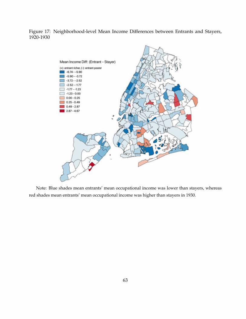
Figure 17: Neighborhood-level Mean Income Differences between Entrants and Stayers,1920-1930
Note: Blue shades mean entrants’ mean occupational income was lower than stayers, whereas
red shades mean entrants’ mean occupational income was higher than stayers in 1930.
63
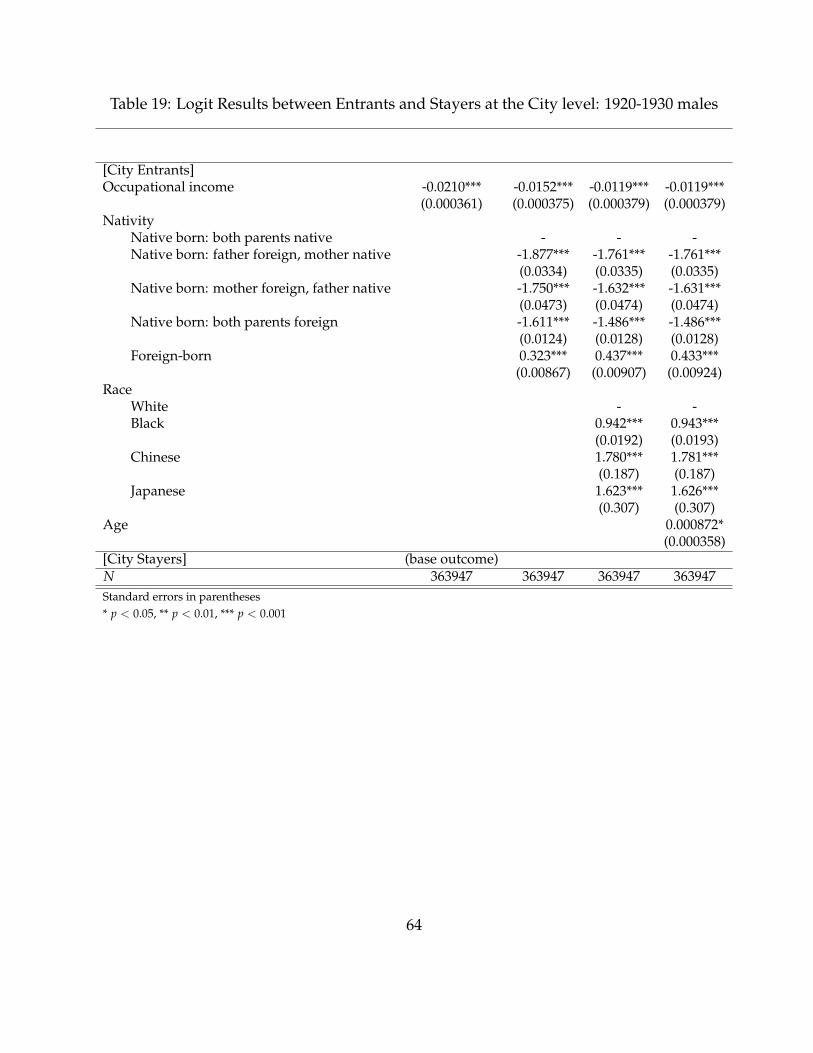
Table 19: Logit Results between Entrants and Stayers at the City level: 1920-1930 males
[City Entrants]Occupational income -0.0210*** -0.0152*** -0.0119*** -0.0119***
(0.000361) (0.000375) (0.000379) (0.000379)Nativity
Native born: both parents native - - -Native born: father foreign, mother native -1.877*** -1.761*** -1.761***
(0.0334) (0.0335) (0.0335)Native born: mother foreign, father native -1.750*** -1.632*** -1.631***
(0.0473) (0.0474) (0.0474)Native born: both parents foreign -1.611*** -1.486*** -1.486***
(0.0124) (0.0128) (0.0128)Foreign-born 0.323*** 0.437*** 0.433***
(0.00867) (0.00907) (0.00924)Race
White - -Black 0.942*** 0.943***
(0.0192) (0.0193)Chinese 1.780*** 1.781***
(0.187) (0.187)Japanese 1.623*** 1.626***
(0.307) (0.307)Age 0.000872*
(0.000358)[City Stayers] (base outcome)N 363947 363947 363947 363947Standard errors in parentheses* p < 0.05, ** p < 0.01, *** p < 0.001
64
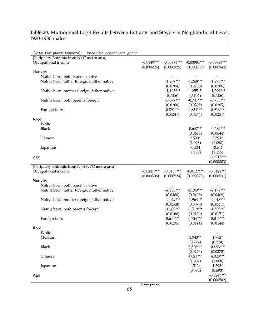
Table 20: Multinomial Logit Results between Entrants and Stayers at Neighborhood Level:1920-1930 males
[City Periphery Stayers]: baseline comparison group[Periphery Entrants from NYC metro area]Occupational income -0.0149*** -0.00873*** -0.00984*** -0.00936***
(0.000924) (0.000925) (0.000939) (0.000940)Nativity
Native born: both parents native - - -Native born: father foreign, mother native -1.207*** -1.268*** -1.276***
(0.0704) (0.0706) (0.0706)Native born: mother foreign, father native -1.193*** -1.255*** -1.299***
(0.106) (0.106) (0.106)Native born: both parents foreign -0.677*** -0.741*** -0.758***
(0.0300) (0.0305) (0.0305)Foreign-born 0.891*** 0.831*** 0.936***
(0.0241) (0.0246) (0.0251)Race
White - -Black -0.647*** -0.685***
(0.0643) (0.0644)Chinese 2.590* 2.591*
(1.098) (1.098)Japanese -0.534 -0.641
(1.155) (1.155)Age -0.0218***
(0.000883)[Periphery Entrants from Non-NYC metro area]Occupational income -0.0227*** -0.0155*** -0.0127*** -0.0122***
(0.000506) (0.000524) (0.000529) (0.000531)Nativity
Native born: both parents native - - -Native born: father foreign, mother native -2.253*** -2.169*** -2.177***
(0.0406) (0.0408) (0.0409)Native born: mother foreign, father native -2.049*** -1.964*** -2.013***
(0.0568) (0.0570) (0.0571)Native born: both parents foreign -1.609*** -1.519*** -1.539***
(0.0166) (0.0170) (0.0171)Foreign-born 0.644*** 0.726*** 0.843***
(0.0135) (0.0141) (0.0144)Race
White - -Mexican 1.943** 1.762*
(0.724) (0.724)Black 0.526*** 0.483***
(0.0273) (0.0275)Chinese 4.023*** 4.023***
(1.007) (1.008)Japanese 1.513* 1.395*
(0.592) (0.593)Age -0.0243***
(0.000502)Continued
65

Table 20: Multinomial Logit Results between Entrants and Stayers at Neighborhood Level:1920-1930 males (cont.)
[City Periphery Stayers]: baseline comparison group[Periphery Entrants from the City’s Core]Occupational income -0.000953* 0.000674 -0.000479 0.000176
(0.000434) (0.000443) (0.000448) (0.000452)Nativity
Native born: both parents native - - -Native born: father foreign, mother native -0.307*** -0.368*** -0.376***
(0.0226) (0.0228) (0.0230)Native born: mother foreign, father native -0.254*** -0.316*** -0.380***
(0.0328) (0.0330) (0.0334)Native born: both parents foreign 0.181*** 0.116*** 0.0883***
(0.0128) (0.0132) (0.0133)Foreign-born 0.447*** 0.387*** 0.545***
(0.0132) (0.0135) (0.0138)Race
White - -Black -0.715*** -0.771***
(0.0304) (0.0306)Chinese 2.330* 2.326*
(1.013) (1.013)Japanese -0.274 -0.424
(0.658) (0.659)Age -0.0325***
(0.000441)N 363947 363947 363947 363947Standard errors in parentheses* p < 0.05, ** p < 0.01, *** p < 0.001
66

Figure 18: Neighborhood-level Mean Income Differences between Entrants and Stayers,1930-1940
Note: Blue shades mean entrants’ mean occupational income was lower than stayers, whereas
red shades mean entrants’ mean occupational income was higher than stayers in 1940.
67

Table 21: Logit Results between Entrants and Stayers at the City level: 1930-1940 males
[City Entrants]Occupational income -0.0111*** -0.00901*** -0.00757*** -0.00792***
(0.00110) (0.00114) (0.00116) (0.00116)Nativity
Native born: both parents native - - -Native born: father foreign, mother native -1.285*** -1.216*** -1.223***
(0.0875) (0.0879) (0.0882)Native born: mother foreign, father native -1.424*** -1.356*** -1.364***
(0.123) (0.123) (0.123)Native born: both parents foreign -1.471*** -1.400*** -1.360***
(0.0342) (0.0352) (0.0354)Foreign-born -0.339*** -0.271*** -0.374***
(0.0278) (0.0289) (0.0300)Race
White - -Black 0.483*** 0.525***
(0.0607) (0.0609)Chinese 0.811 0.898
(0.524) (0.523)Japanese -14.13 -13.86
(693.0) (611.5)Age 0.0163***
(0.00117)[City Stayers] (base outcome)N 169642 169642 169642 169642Standard errors in parentheses* p < 0.05, ** p < 0.01, *** p < 0.001
68
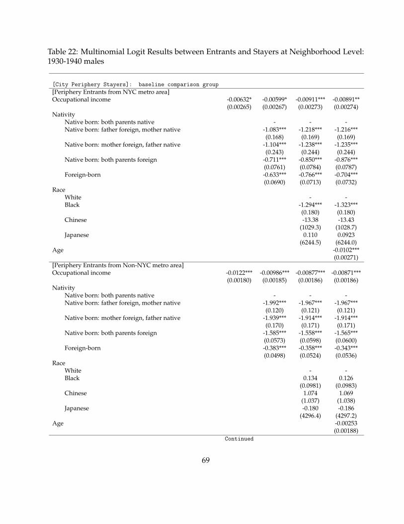
Table 22: Multinomial Logit Results between Entrants and Stayers at Neighborhood Level:1930-1940 males
[City Periphery Stayers]: baseline comparison group[Periphery Entrants from NYC metro area]Occupational income -0.00632* -0.00599* -0.00911*** -0.00891**
(0.00265) (0.00267) (0.00273) (0.00274)Nativity
Native born: both parents native - - -Native born: father foreign, mother native -1.083*** -1.218*** -1.216***
(0.168) (0.169) (0.169)Native born: mother foreign, father native -1.104*** -1.238*** -1.235***
(0.243) (0.244) (0.244)Native born: both parents foreign -0.711*** -0.850*** -0.876***
(0.0761) (0.0784) (0.0787)Foreign-born -0.633*** -0.766*** -0.704***
(0.0690) (0.0713) (0.0732)Race
White - -Black -1.294*** -1.323***
(0.180) (0.180)Chinese -13.38 -13.43
(1029.3) (1028.7)Japanese 0.110 0.0923
(6244.5) (6244.0)Age -0.0102***
(0.00271)[Periphery Entrants from Non-NYC metro area]Occupational income -0.0122*** -0.00986*** -0.00877*** -0.00871***
(0.00180) (0.00185) (0.00186) (0.00186)Nativity
Native born: both parents native - - -Native born: father foreign, mother native -1.992*** -1.967*** -1.967***
(0.120) (0.121) (0.121)Native born: mother foreign, father native -1.939*** -1.914*** -1.914***
(0.170) (0.171) (0.171)Native born: both parents foreign -1.585*** -1.558*** -1.565***
(0.0573) (0.0598) (0.0600)Foreign-born -0.383*** -0.358*** -0.343***
(0.0498) (0.0524) (0.0536)Race
White - -Black 0.134 0.126
(0.0981) (0.0983)Chinese 1.074 1.069
(1.037) (1.038)Japanese -0.180 -0.186
(4296.4) (4297.2)Age -0.00253
(0.00188)Continued
69
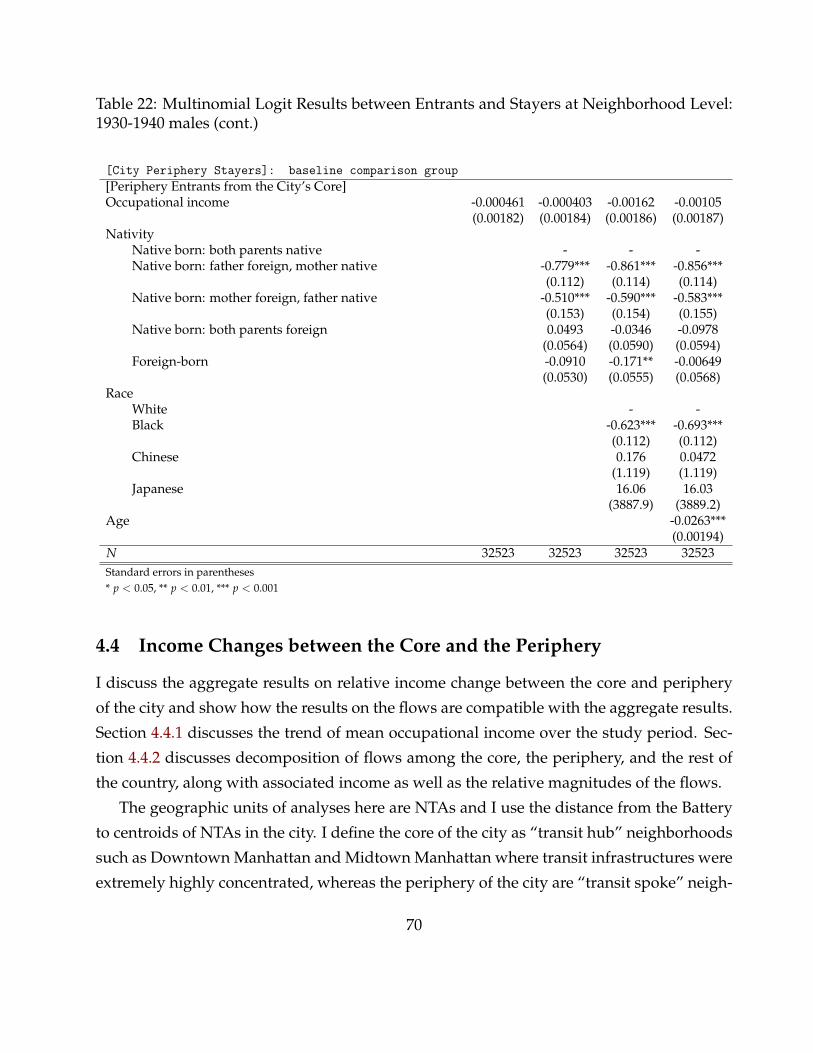
Table 22: Multinomial Logit Results between Entrants and Stayers at Neighborhood Level:1930-1940 males (cont.)
[City Periphery Stayers]: baseline comparison group[Periphery Entrants from the City’s Core]Occupational income -0.000461 -0.000403 -0.00162 -0.00105
(0.00182) (0.00184) (0.00186) (0.00187)Nativity
Native born: both parents native - - -Native born: father foreign, mother native -0.779*** -0.861*** -0.856***
(0.112) (0.114) (0.114)Native born: mother foreign, father native -0.510*** -0.590*** -0.583***
(0.153) (0.154) (0.155)Native born: both parents foreign 0.0493 -0.0346 -0.0978
(0.0564) (0.0590) (0.0594)Foreign-born -0.0910 -0.171** -0.00649
(0.0530) (0.0555) (0.0568)Race
White - -Black -0.623*** -0.693***
(0.112) (0.112)Chinese 0.176 0.0472
(1.119) (1.119)Japanese 16.06 16.03
(3887.9) (3889.2)Age -0.0263***
(0.00194)N 32523 32523 32523 32523Standard errors in parentheses* p < 0.05, ** p < 0.01, *** p < 0.001
4.4 Income Changes between the Core and the Periphery
I discuss the aggregate results on relative income change between the core and peripheryof the city and show how the results on the flows are compatible with the aggregate results.Section 4.4.1 discusses the trend of mean occupational income over the study period. Sec-tion 4.4.2 discusses decomposition of flows among the core, the periphery, and the rest ofthe country, along with associated income as well as the relative magnitudes of the flows.
The geographic units of analyses here are NTAs and I use the distance from the Batteryto centroids of NTAs in the city. I define the core of the city as “transit hub” neighborhoodssuch as Downtown Manhattan and Midtown Manhattan where transit infrastructures wereextremely highly concentrated, whereas the periphery of the city are “transit spoke” neigh-
70
borhoods such as Upper Manhattan and outer boroughs of the city.
4.4.1 Occupational income
Figure 19 reveals that the mean occupational income decreases as the distance from theBattery increases while the slope of fitted values getting more flat from 1870 to 1900. In1910, this slope stays flat, and then in 1920, the mean occupational income slightly increasesas the distance from the Battery increases. In Years 1930 and 1940, the slope becomes evensteeper, implying that the mean occupational income at the edge (relative to the center) ofthe city increases even further. Over time, the relative income was higher in the center ofthe city (relative to the periphery) in the first half of the study period, whereas the relativeincome in the periphery became higher in the second half of the study period.
Figure 20 shows that the percent change of mean occupation income gets higher as itgets further away from the center. However, note that in the earlier study period (till 1900),mean occupational income was increasing both at the center and the edge whereas, during1910 and 1930, percent change of mean occupational income was negative at the centerwhich means the mean occupational income was decreasing at the center of the city. Atthe very end of the study period (i.e. 1930-1940), the curve becomes close to nil both at thecenter and edge, implying that the mean occupational income almost stayed the same asthe earlier decade.
71

Figure 19: Mean Occupational Income
(a) 1870
1820
2224
2628
Mea
n(O
ccup
atio
nal I
ncom
e)
0 10 20 30Distance from the Battery (in kilometer)
(mean) occscore Fitted values
72

Figure 19: Mean Occupational Income
(b) 1880
2122
2324
2526
Mea
n(O
ccup
atio
nal I
ncom
e)
0 10 20 30Distance from the Battery (in kilometer)
(mean) occscore Fitted values
(c) 1900
1820
2224
2628
Mea
n(O
ccup
atio
nal I
ncom
e)
0 10 20 30Distance from the Battery (in kilometer)
(mean) occscore Fitted values
73

Figure 19: Mean Occupational Income
(d) 1910
1520
2530
Mea
n(O
ccup
atio
nal I
ncom
e)
0 10 20 30Distance from the Battery (in kilometer)
(mean) occscore Fitted values
(e) 1920
1520
2530
35M
ean(
Occ
upat
iona
l Inc
ome)
0 10 20 30Distance from the Battery (in kilometer)
(mean) occscore Fitted values
74
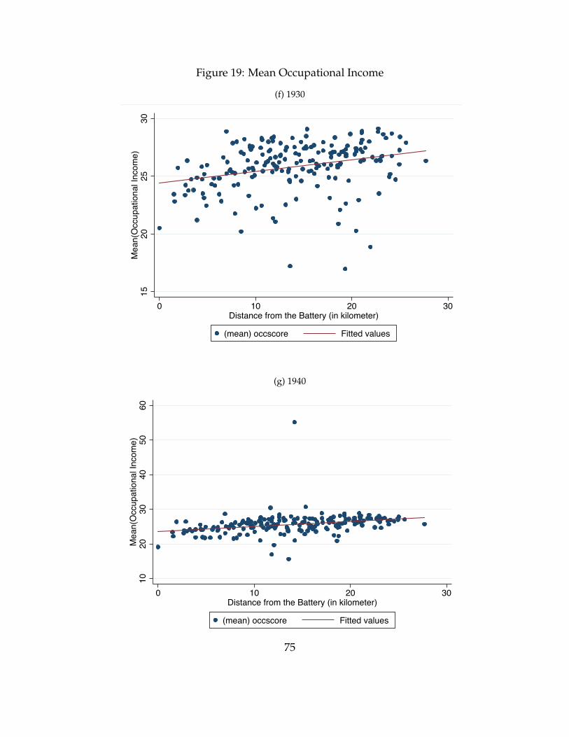
Figure 19: Mean Occupational Income
(f) 1930
1520
2530
Mea
n(O
ccup
atio
nal I
ncom
e)
0 10 20 30Distance from the Battery (in kilometer)
(mean) occscore Fitted values
(g) 1940
1020
3040
5060
Mea
n(O
ccup
atio
nal I
ncom
e)
0 10 20 30Distance from the Battery (in kilometer)
(mean) occscore Fitted values
75

Figure 20: % Change of Mean Occupational Income
(a) 1880-1900
-10
010
2030
% C
hang
e of
Mea
n O
ccup
atio
nal I
ncom
e
0 10 20 30Distance from the Battery (in kilometer)
% change mean income b/w 1880, 1900 Fitted values
(b) 1900-1910
-40
-20
020
40%
Cha
nge
of M
ean
Occ
upat
iona
l Inc
ome
0 10 20 30Distance from the Battery (in kilometer)
% change mean income b/w 1900, 1910 Fitted values
76

Figure 20: % Change of Mean Occupational Income
(c) 1910-1920
-20
-10
010
2030
40%
Cha
nge
of M
ean
Occ
upat
iona
l Inc
ome
0 10 20 30Distance from the Battery (in kilometer)
% change mean income b/w 1910, 1920 Fitted values
(d) 1920-1930
-30
-10
1030
5070
90%
Cha
nge
of M
ean
Occ
upat
iona
l Inc
ome
0 10 20 30Distance from the Battery (in kilometer)
% change of mean income b/w 1920, 1930 Fitted values
77
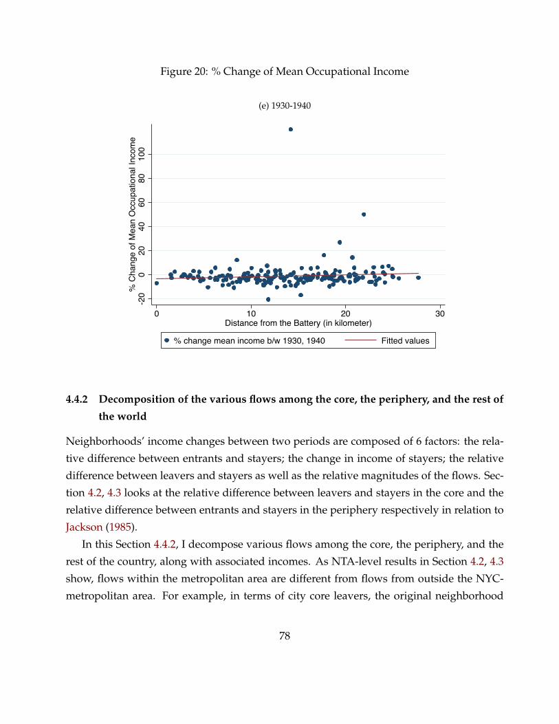
Figure 20: % Change of Mean Occupational Income
(e) 1930-1940
-20
020
4060
8010
0%
Cha
nge
of M
ean
Occ
upat
iona
l Inc
ome
0 10 20 30Distance from the Battery (in kilometer)
% change mean income b/w 1930, 1940 Fitted values
4.4.2 Decomposition of the various flows among the core, the periphery, and the rest ofthe world
Neighborhoods’ income changes between two periods are composed of 6 factors: the rela-tive difference between entrants and stayers; the change in income of stayers; the relativedifference between leavers and stayers as well as the relative magnitudes of the flows. Sec-tion 4.2, 4.3 looks at the relative difference between leavers and stayers in the core and therelative difference between entrants and stayers in the periphery respectively in relation toJackson (1985).
In this Section 4.4.2, I decompose various flows among the core, the periphery, and therest of the country, along with associated incomes. As NTA-level results in Section 4.2, 4.3show, flows within the metropolitan area are different from flows from outside the NYC-metropolitan area. For example, in terms of city core leavers, the original neighborhood
78

residents leaving to the periphery of the city may be different (in terms of income and othercharacteristics such as age and race) from residents leaving to NYC metropolitan area suchas Westchester County, or residents moving to outside NYC metro area entirely. Similarly,entrants to the periphery neighborhood in the city could be from another neighborhood inthe city including the core of the city (as Jackson (1985) discussed), or from NYC metro area(e.g. Westchester county located in the north of NYC which is a part of NYC metro area), orfrom outside NYC metro area.
Specifically, I decompose the changes in the core and the periphery in the followingway. In terms of the core, I look at various flows including the relative income differencebetween leavers and stayers as well as the corresponding relative magnitudes of those flowsat the neighborhood level. In terms of the periphery, I look at various flows includingthe relative income difference between entrants and stayers as well as the correspondingrelative magnitudes of those flows at the neighborhood level.
These decomposition analyses are complementary to results in Table 4, 6, 8, 10, 12 forleavers (relative to stayers at the neighborhood level) at the core of the city, and in Table 14,16, 18, 20, 22 for entrants (relative to stayers at the neighborhood level) at the periphery ofthe city.
I look separately at flows within the city, flows within the metro area, and flows fromthe outside the metro area in analyzing neighborhood changes at the neighborhood level.
• Decomposition of the core of the city (leavers and stayers at the core of the city)
I decompose various flows of the core of the city including the relative income differencebetween leavers and stayers as well as the corresponding relative magnitudes of those flowsat the neighborhood level. In Figure 21, the size of hollow circle denotes that relative ratioof such migration-type, whereas y-axis indicates the mean occupational income of eachmigration type. In Figure 21, as x-axis captures the number of flows, strictly positive signindicates inflows (entrants) whereas strictly negative sign indicates outflows (leavers), andthe distance away from 0 captures the total number of flows across migration-type.
Throughout the study period, neighborhood stayers at the core (in Lavender in Figures21a, 21c, 21e, 21g) had the highest mean occupational income relative to other neighborhoodleavers at a varying degree. Related to Jackson (1985), core leavers to the periphery in thecity (in Cranberry) and to NYC metro area (in Orange) relative to the core stayers matter.
79

Figures 21a, 21c, 21e, 21g show the core stayers’ income (in Lavender) was higher than thosetwo groups throughout the study period. This is consistent with my findings in Section 4.2that it was not the rich who left the center of the city. However, although the neighborhoodstayer at the core may have been the richest, only a small fraction of people stayed in thesame neighborhood and the majority of them left the core of the city — some migratedto the periphery of the city, others migrated to NYC metro area, and the others migratedoutside the NYC metro area at all.
The relative magnitude of flows gives us a richer story regarding the evolution of thecore of the city. First of all, till 1910, the proportion of leavers who are leaving to outsideNYC metro area (in Teal) was higher than any other group, whereas starting in 1920, theproportion of neighborhood leavers moving to the periphery in the city became higher thanany other group. This implies the magnitude of within-city internal migration increasedgreatly around 1920 which was at the peak of intra-city transit infrastructure investmentafter the Dual Contract. It is also notable that between Years 1920 and 1930, the magnitudeof leavers to the periphery of the city and is astonishing — the number of leavers who wereleaving the core of the city were almost five times bigger than the number of entrants tothe core — implying that population decline in the core of the city was more dramatic thanever.
Therefore, although Jackson (1985)’s fundamental claim about the growth of high in-come at the edge relative to the center holds true for my study (which I will discuss in thefollowing decomposition), Jackson (1985)’s claim of the rich leaving the center of the city asthe mechanism for explaining the growth of high income at the edge does not hold true formy study. Jackson’s straightforward inference of the rich leaving the center and moving tothe periphery does not apply to my longitudinal data-based migration analysis. To recap,the core stayers were richer than any other leaver groups at any destination, and it was notthe rich who left the core of the city.
The flows of entrants also capture how the change — change of incomes at the centerdeclining relative to the center — actually happened. The core entrants’ income was muchlower than leavers and this is especially pronounced for core entrants from outside NYCmetro area (in Maroon). Entrants from outside NYC metro area were the largest entrantgroup with the lowest mean income, and therefore, this must have caused the core of thecity’s income to decrease.
80

To recap, the transit changes in my study period had a similar nature of Jackson (1985)and the postwar period and incomes at the edge were rising relative to the center. However,the mechanism behind these changes was not a simple shuffling of the rich and poor.
• Decomposition of the periphery of the city (entrants and stayers at the periphery ofthe city)
I also decompose various flows of the periphery of the city including the relative incomedifference between entrants and stayers as well as the corresponding relative magnitudes ofthose flows at the neighborhood level. Throughout the study period, neighborhood stayersat the periphery of the city (in Lavender in Figures 21b, 21d, 21f, 21h, 21j) had a highermean occupational income than other periphery entrant groups. Related to Jackson (1985),the income of periphery entrants from the core (in Maroon) relative to periphery stayersmatter. Figures 21b, 21d, 21f, 21h, 21j show that income of the periphery entrants from thecore (in Maroon) was lower than that of periphery stayers (in Lavender) throughout mystudy period.
Therefore, Jackson (1985)’s straightforward inference about the rich from the core mov-ing to the periphery as the primary mechanism for the edge’s relative income growth doesnot hold for my study. The periphery entrants from the city core had lower mean incomethan periphery stayers, and their relative magnitude in terms of the number of people wasfairly small. The primary mechanism behind the income growth are three forces: 1. the pe-riphery leavers moving to outside New York metro area had lowest mean income than anyother group, and they left the city periphery greatly (in Cranberry), 2. periphery entrantsfrom outside NYC metro area (in Green) had much higher mean income than peripheryleavers and magnitude of this inflow was big enough to dominate all the other forces, 3. theperiphery stayers’ income increased substantially (Figure 22b).
To summarize, incomes at the periphery were rising relative to the center due to entrantsfrom outside NYC metro area with a higher income than periphery leavers and this flowwas sizable both in terms of the relative income difference between leavers and entrants aswell as the relative magnitudes of the flows.
Finally, the decomposition analyses show that the neighborhood stayers at the peripherywere not poorer than most entrants into the periphery. However, Table 14, 16, 18, 20, 22
81

show that the new suburbanites at the periphery were not richer than the people who stayedat the periphery.
82

Figure 21: Mean Income and Magnitude of Flows Across Migration-type: 1880-1900
(a) Core Flows from 1880-1900 panel
(b) Periphery Flows From 1880-1900 panel
83

Figure 21: Mean Income and Magnitude of Flows Across Migration-type: 1900-1910
(c) Core Flows from 1900-1910 panel
(d) Periphery Flows From 1900-1910 panel
84
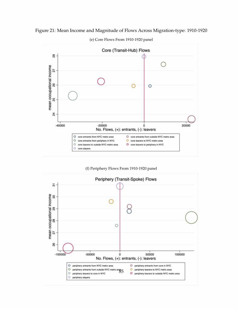
Figure 21: Mean Income and Magnitude of Flows Across Migration-type: 1910-1920
(e) Core Flows From 1910-1920 panel
(f) Periphery Flows From 1910-1920 panel
85

Figure 21: Mean Income and Magnitude of Flows Across Migration-type: 1920-1930
(g) Core Flows From 1920-1930 panel
(h) From 1920-1930 panel
86

Figure 21: Mean Income and Magnitude of Flows Across Migration-type: 1930-1940
(i) Core Flows From 1930-1940 panel
(j) Periphery Flows From 1930-1940 panel
87
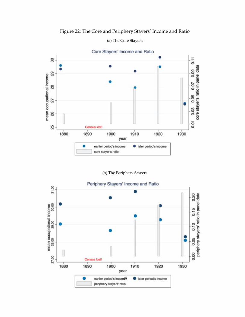
Figure 22: The Core and Periphery Stayers’ Income and Ratio
(a) The Core Stayers
(b) The Periphery Stayers
88
5 Conclusion
With the 21st-century advanced techniques and computational power, I construct longitu-dinal database by linking complete-count US census records from 1870 to 1940. I analyzeincome and socioeconomic status of individuals who lived in the New York City and ana-lyze whether the dynamic process of suburbanization in New York systematically differedfor the poor and rich (and other characteristics).
Longitudinal data reveal that in the core, it was not the case either that rich people leftor that poor people stayed; in the periphery, people who moved into the periphery werenot richer than original residents. The suburbanization in prewar New York was probablydifferent from postwar suburbanization. The people who lived in the central city were notpoor; those who left were not more affluent.
My study period also captures the growth of high income at the periphery relative tothe center as in Jackson (1985)’s period (1815-1875) and the postward period. However,unlike other works that do not use panel data, I use panel data of individuals to uncoverthe mechanism behind the growth of high income at the edge relative to the center. Insteadof making an inference about who moved, left, and stayed, I show how the change actuallyhappened.
Essentially, the transit infrastructure improvements and changes in my study period hadthe same nature of Jackson’s period and the post war period—incomes at the edge risingrelative to the center. However, the anatomy of how this change actually happened showsthat incomes rising at the edge (relative to the center) was not a simple shuffling of richand poor. Up until the Great Depression, flows of migrants from and to outside the NYCmetropolitan area were the dominant force in changing average income. Richer peoplefrom outside migrated to the periphery, whereas poorer people from outside migrated tothe core. The people from the core who left the NYC metropolitan area entirely were richerthan the people from the periphery who left the NYC metropolitan area. Finally, peoplewho stayed at the periphery got richer as the metropolis grew.
Finally, while this paper quantitatively shows the dynamic process of suburbanizationin relations to transit infrastructure improvement, it still is not clear whether the welfareconsequences differ across the rich and the poor (or high skill and low skill workers). Ana-lyzing rigorous welfare comparisons offers a direction for future research.
89

References
AHLFELDT, G. M., S. J. REDDING, D. M. STURM, AND N. WOLF (2012): “The Economicsof Density: Evidence from the Berlin Wall,” CEP Discussion Papers dp1154, Centre forEconomic Performance, LSE. 1
ALLEN, T. AND C. ARKOLAKIS (2013): “Trade and the Topography of the Spatial Economy,”NBER Working Papers 19181, National Bureau of Economic Research, Inc. 1
——— (2015): “A Model of Trade and Migration,” Working paper. E
ALLEN, T., C. ARKOLAKIS, AND X. LI (2015): “Optimal City Structure,” Working papers,Yale University. 1
ALLEN, T., C. D. C. DOBBIN, AND M. MORTEN (2018): “Border Walls,” Working Paper25267, National Bureau of Economic Research. E
ALONSO, W. (1964): Location and land use. Toward a general theory of land rent., Cambridge,Mass.: Harvard Univ. Pr. 10
BANERJEE, A., E. DUFLO, AND N. QIAN (2012): “On the Road: Access to TransportationInfrastructure and Economic Growth in China,” NBER Working Papers 17897, NationalBureau of Economic Research, Inc. 1
BAUM-SNOW, N. (2007): “Did Highways Cause Suburbanization?” Tech. Rep. 2. 1, 1
BOUSTAN, L. P. (2010): “Was Postwar Suburbanization “White Flight"? Evidence from theBlack Migration,” The Quarterly Journal of Economics, 125, 417–443. 1
DONALDSON, D. (2010): “Railroads of the Raj: estimating the impact of transportationinfrastructure,” LSE Research Online Documents on Economics 38368, London School ofEconomics and Political Science, LSE Library. 1
DONALDSON, D. AND M. HORNBECK (2013): “Railroads and American Economic Growth:A "Market Access" Approach,” NBER Working Papers 19213, National Bu-reau of Economic Research, Inc. 1
90

DURANTON, G., P. MORROW, AND M. TURNER (2013): “Roads and Trade: Evidence fromthe U.S,” Working Papers tecipa-479, University of Toronto, Department of Economics. 1
ELLEN, I. G. AND K. O’REGAN (2011): “How low income neighborhoods change: Entry,exit, and enhancement,” Regional Science and Urban Economics, 41, 89–97. 2.1.1
FABER, B. (2013): “Trade Integration, Market Size and Industrialization: Evidence fromChina’s National Trunk Highway System,” CEP Discussion Papers dp1244, Centre forEconomic Performance, LSE. 1
FEIGENBAUM, J. J. (2015): “Intergenerational Mobility during the Great Depression,” . 2.2,B.1
FUJITA, M. AND H. OGAWA (1982): “Multiple equilibria and structural transition of non-monocentric urban configurations,” Tech. Rep. 2. 1
GILMAN, L. P. (1971): “The Development of a Neighborhood: Bedford, 1850-1880: A. CaseStudy,” Master’s thesis, columbia university. 14
GOEKEN, R., L. HUYNH, T. LYNCH, AND R. VICK (2011): “New methods of census recordlinking,” Historical methods, 44, 7–14. 2.2, B.1, B.1
HEBLICH, S., S. REDDING, AND D. M. STURM (2018): “The Making of the Modern Metropo-lis: Evidence from London,” Working Paper 25047, National Bureau of Economic Re-search. 1
JACKSON, K. T. (1985): Crabgrass Frontier: The Suburbanization of the United States, OxfordUniversity Press, USA. 1, 1, 2.1.2, 4.2, 4.3, 14, 4.4.2, 5, 18
LUCAS, R. E. AND E. ROSSI-HANSBERG (2002): “On the Internal Structure of Cities,” Tech.Rep. 4. 1
MICHAELS, G. (2008): “The Effect of Trade on the Demand for Skill: Evidence from theInterstate Highway System,” The Review of Economics and Statistics, 90, 683–701. 1
MILLS, E. S. (1967): “An Aggregative Model of Resource Allocation in a MetropolitanArea,” The American Economic Review, 57, 197–210. 10
91

MONTE, F., S. J. REDDING, AND E. ROSSI-HANSBERG (2015): “Commuting, Migration andLocal Employment Elasticities,” CEP Discussion Papers dp1385, Centre for EconomicPerformance, LSE. 1
MUTH, R. F. (1964): Cities and Housing: The Spatial Pattern of Urban Residential Land Use., TheUniversity of Chicago Press. 10
RUGGLES, S., S. FLOOD, R. GOEKEN, J. GROVER, E. MEYER, J. PACAS, AND M. SOBEK
(2019): “IPUMS USA: Version 9.0 [dataset],” Minneapolis, MN: IPUMS, https://doi.org/10.18128/D010.V10.0 2.1, 2.1.1, 2.5
SHERTZER, A., R. P. WALSH, AND J. R. LOGAN (2016): “Segregation and Neighborhood Change in Northern Cities: New Historical GIS Data from 1900 to 1930,” Tech. rep. 2.3
TSIVANIDIS, N. (2018): “The Aggregate And Distributional Effects Of Urban Transit Infras-tructure: Evidence From Bogotá’s TransMilenio,” . 1
92

A Appendix
93

Appendix to Chapter 1
In this section, I describe the record linking procedure and relevant details. In constructing apanel of individuals, I use “Machine Learning,” where the machine can learn the pattern of“true” and “false” matches and self-link individuals after learning the patterns of true andfalse matches from training datasets. This method is implemented to link individuals acrosscensus years while maximizing the match rate and representativeness of linked datasets. Ilink complete-count US Federal Decennial Demographic Census records from 1850 to 1940with newly transcribed socioeconomic variables such as occupation and industry.
B Methodology
B.1 Machine Learning Approach of Record MatchingThe “machine learning” approach for record linking borrows insights from computer sci-ence and statistics and I implement this method of classification and text comparison to linkindividual records. The rationale behind my choice of machine learning is to learn frombig data. In essence, record linking without unique identifier is to predict whether certainlinked records are “true” links of the same individual or not, based on a set of features suchas first name and last name, age, and place of birth. Similar efforts have been pioneered byGoeken et al. (2011) that create the IPUMS linked samples. Feigenbaum (2015) links indi-vidual records of the 1915 Iowa State Census to their adult-selves in the 1940 US FederalDemographic Census records. Relative to the mentioned work, my record linking is farmore extensive in the scope of matching as this involves complete-count US Federal Decen-nial Demographic Census records of all years from 1850 to 1940. I teach a machine to learnto predict based on a set of features. I create a training dataset in which contain both “true”and “false” matches and their characteristics (e.g some observations with “true” as an out-come would have same/very similar characteristics in terms of age, first and last name, par-ents’ and his/her birthplaces whereas observations with “false” as an outcome would havequite different characteristics in terms of the above mentioned characteristics). In this case,the outcome is whether the matched records are “true” or “false” match, given the observedcharacteristics. By taking this training data, I build a prediction model, or learner, whichwill enable us to predict the outcome for new, unseen objects. A well-designed learnerarmed with a solid training dataset should accurately predict outcomes for new unseenobjects.
I implement a supervised learning problem in the sense that the presence of outcomevariable (“true” or “false” links) guides the learning process—in other words, the end-goalis to use the inputs to predict the output values. To summarize this process, I extract sub-sets of possible matches for each record and create training data in order to tune a matchingalgorithm so that the matching algorithm matches individual records by minimizing bothfalse positives and false negatives while reflecting inherent noises in historical records. I
94

have explored various models for model selection. By comparing and analyzing matchedrecords that I match through various methods, I choose the random forest classification asit is more conservative in matching records—the number of matched records is lower thanthat of Support Vector Machine (hereafter, SVM)— and the number of unique matches aresignificantly higher than the standard SVM model. Although the choice of random forestclassification may result in lower number match rate due to its conservative nature, I inte-grated household-level information in linking individual records to mitigate the concernsof low match rate.
A filtering process called “pruning” for non-unique matches
Although I largely follow the standard machine-learning record linking methodology sug-gested by Goeken et al. (2011), I have extended the techniques of Goeken et al. (2011) byinventing a two-step machine learning matching methodology. Especially, I make use ofthe parents and/or spouse information such as birthplaces and names to choose the “true”match among other candidate matches. This additional step of extracting household-levelinformation and its use in selecting “true” matches among multiple candidates (insteadof dropping non-unique matches, which have been the “standard” practices in the exist-ing record matching literature) is novel. This procedure can not only save a number ofmatches that otherwise had to be dropped but also correct for the selection bias (peoplewith common characteristics such as common first and last names may be systematicallyunder-represented in linked datasets).
B.2 Record Linking in Practice: InnovationsThe core of census matching is a classification problem. Given any pair of records fromdifferent census years, finding a true match is to find the mapping that classifies the pairas matched or unmatched based on the set of pre-determined features, including names,gender, age, race and birthplace. However, since this set of features is far from unique,there are cases where one individual has several candidate matches (e.g. there are many“John Smith” with same age).
Most record linking approaches throw away non-unique matches. One of the contribu-tions of my record linking approach is the use of household-level information to turn thenon-unique types of matches (second to fourth type) as unique matches. Specifically, I usefather and mother’s information such as their racial background, birthplaces, birth year)and use the same information for spouses of individuals. This not only increases the matchrates but also alleviates the concern of systematic selection bias (e.g. people with commongiven given and last names may be systematically under-represented in the linked data).
95

B.2.1 Female Record Linking
Historically, as women typically change their last names after marriage (and in the absenceof time-invariant individual-level unique identifiers such as social security number in his-torical records), female record linking has been challenging. To my knowledge, this is oneof the first endeavors of linking historical female records. I assume that women’s last namesare likely to change if their marital status changes from single in the earlier period to mar-ried in the later period, and I do not consider record linking for such case. On the otherhand, I assume one’s last name is likely to remain the same if the marital status is eithermarried to the same partner in both years, or married in the early period and then wid-owed or divorced in the later period; or remained single in both periods.
C The Transportation RevolutionTransit infrastructure improved dramatically at both intra- and inter-city level during thestudy period. Figure 23 shows the total number of intra-city railways and subway stationsby borough by the end of each decade during the study period. Especially, during thesubway construction period between 1904 and 1920, the total number of stations grew by200% and 113% in the Bronx, 87% and 105% in Brooklyn, 50% and 133% in Queens.
Inter-city transit infrastructure improvements at an unprecedented scale during the studyperiod as well: electrification of railroads that served central Westchester county, Connecti-cut in 1907 and 1914 improved the efficiency and speed of railways greatly, the HudsonTubes that connected New Jersey was built in 1908, and inter-city railway that connectedNYC to the rest of the country with the opening of Penn Station in 1910.
C.1 Intra-city transit infrastructure changes• Subways and Elevated Railways Construction and Network Change over Time
96

Figure 23: Total number of intra-city railway, subway stations
Source: Author’s creation using New York Transit Museum Archive.
Figure 24 captures the evolution of spatial links by intra-city commuting transit infras-tructure which are the elevated and subterranean railways. Before the introduction of thesubway in 1904, New York City had a large central business district in lower Manhattanand a smaller business district in downtown Brooklyn. These districts were served by ele-vated railways and ferries and most of the services were operating in Manhattan. As Figure24 shows, elevated lines ran north from the southern tip of Manhattan to the Bronx. Therewere very few east-west connections in Manhattan and this pattern persisted for the sub-way network in the twentieth century as well. Before the introduction of the subway in1904, Manhattan was the only borough with rapid mass transit commuting infrastructure.Most outer boroughs (i.e. Queens, Staten Island, and the Bronx) did not have transit net-work into the 1910s and were semi-rural and underdeveloped. Figure 23 shows the totalnumber of stations by the borough over time. The first decade of subway constructionmostly served Manhattan and Brooklyn, whereas parts of Bronx, Queens and South Brook-lyn received more subway constructions in the 1910s under the Dual Contracts. However,the rapid growth of the system largely was over by 1940.16
16The first underground line of the subway opened in 1904, almost 40 years after the opening of the firstelevated railway in Manhattan. New York City subway was built by two private companies (the BrooklynRapid Transit Company (BRT, later Brooklyn–Manhattan Transit Corporation, BMT) and the InterboroughRapid Transit Company (IRT)) and one city-owned company (Independent Subway System (IND)). In 1940,
97

• Intra-city transit access measures by the elevated railways and subways
I define Transit Access (hereafter, TA) as the number of stations in each neighborhood.17 Thenumber of total stations as a proxy for transit access is convenient in understanding a formof hub-spoke distribution paradigm where a series of “spokes” that connect outlying pointsto a central “hub.” Before the introduction of subways, lower Manhattan (“DowntownManhattan”) was the area where the transit network is extremely well connected (“transithubs”). However, as subway expanded and inter-city transit infrastructure was largely builtin Midtown Manhattan, “transit hubs” expanded from Downtown Manhattan to MidtownManhattan. I describe the spatial links by inter-city transit infrastructure in the followingSubsubsection C.2.
the city bought the two private systems and consolidated the transit network.17In the Appendix, I map transit access change over the study period based on intra-city mass transit in-
frastructure (i.e. the elevated railways and subways)
98

Figure 24: Evolution of Spatial Links by the Elevated Railway, Subways
Note: The above figures show the evolution of intra-city spatial links in terms of the elevated railway, subwaysover study period. Different colors denote the opening years of transit links. Source: Author’s Creation usingNew York City Department of City Planning’s data called “LION” GIS data which is a base map representingthe city’s geographic features.
• Transit access changes based on the elevated railway and subway
99

Figure 25: The Els, Subways-Based Transit Access Measures by Decade
(a) Transit Access in 1900
(b) Transit Access in 1910 (c) Transit Access in 1920
(d) Transit Access in 1930 (e) Transit Access in 1940
Note: The above figures show transit access by decade based on intra-city mass transit infrastructure(i.e. the elevated railways and subways).
100
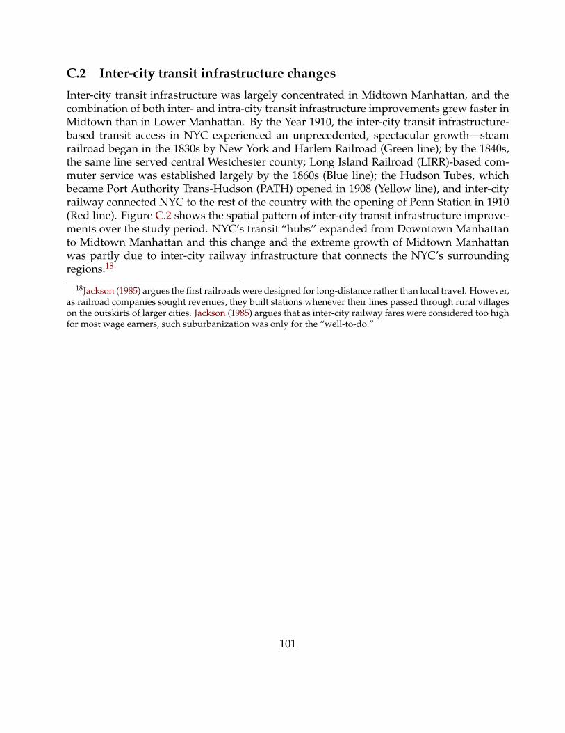
C.2 Inter-city transit infrastructure changesInter-city transit infrastructure was largely concentrated in Midtown Manhattan, and thecombination of both inter- and intra-city transit infrastructure improvements grew faster inMidtown than in Lower Manhattan. By the Year 1910, the inter-city transit infrastructure-based transit access in NYC experienced an unprecedented, spectacular growth—steamrailroad began in the 1830s by New York and Harlem Railroad (Green line); by the 1840s,the same line served central Westchester county; Long Island Railroad (LIRR)-based com-muter service was established largely by the 1860s (Blue line); the Hudson Tubes, whichbecame Port Authority Trans-Hudson (PATH) opened in 1908 (Yellow line), and inter-cityrailway connected NYC to the rest of the country with the opening of Penn Station in 1910(Red line). Figure C.2 shows the spatial pattern of inter-city transit infrastructure improve-ments over the study period. NYC’s transit “hubs” expanded from Downtown Manhattanto Midtown Manhattan and this change and the extreme growth of Midtown Manhattanwas partly due to inter-city railway infrastructure that connects the NYC’s surroundingregions.18
18Jackson (1985) argues the first railroads were designed for long-distance rather than local travel. However,as railroad companies sought revenues, they built stations whenever their lines passed through rural villageson the outskirts of larger cities. Jackson (1985) argues that as inter-city railway fares were considered too highfor most wage earners, such suburbanization was only for the “well-to-do.”
101

Figure 26: Evolution of Inter-City Transit Infrastructure by Construction Year
Note: The above figure shows the evolution of inter-city transit networks by railroad network and construc-tion year. I construct the following information based on information provided by the New York City TransitAuthority and related books (http://www.mta.info/).
• Bridges, Ferries, and Tunnels
Although the railway is my primary focus of the study, water-borne transportation playedan important role in forming connections between the core and connecting regions such asBrooklyn, Staten Island, and parts of New Jersey. As the city economy depended on water-borne transport, extensive bridge-building followed: the Brooklyn Bridge (1883), Williams-burg Bridge (1903), Manhattan Bridge (1909), and Queensboro Bridge (1909) were con-structed over the East River. The Hell Gate Bridge (1917) carried trains of the Pennsyl-vania Railroad and finally, George Washington Bridge (1931) connected New Jersey andNew York City. In the Appendix, I map bridges, ferries, and tunnels that were constructed
102
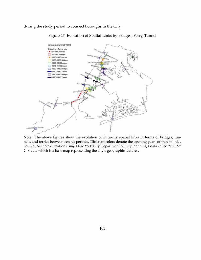
during the study period to connect boroughs in the City.
Figure 27: Evolution of Spatial Links by Bridges, Ferry, Tunnel
Note: The above figures show the evolution of intra-city spatial links in terms of bridges, tun-nels, and ferries between census periods. Different colors denote the opening years of transit links.Source: Author’s Creation using New York City Department of City Planning’s data called “LION”GIS data which is a base map representing the city’s geographic features.
103
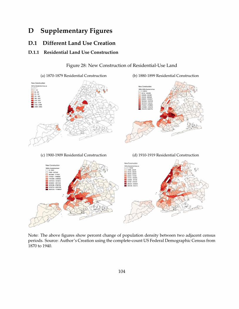
D Supplementary Figures
D.1 Different Land Use CreationD.1.1 Residential Land Use Construction
Figure 28: New Construction of Residential-Use Land
(a) 1870-1879 Residential Construction (b) 1880-1899 Residential Construction
(c) 1900-1909 Residential Construction (d) 1910-1919 Residential Construction
Note: The above figures show percent change of population density between two adjacent censusperiods. Source: Author’s Creation using the complete-count US Federal Demographic Census from1870 to 1940.
104
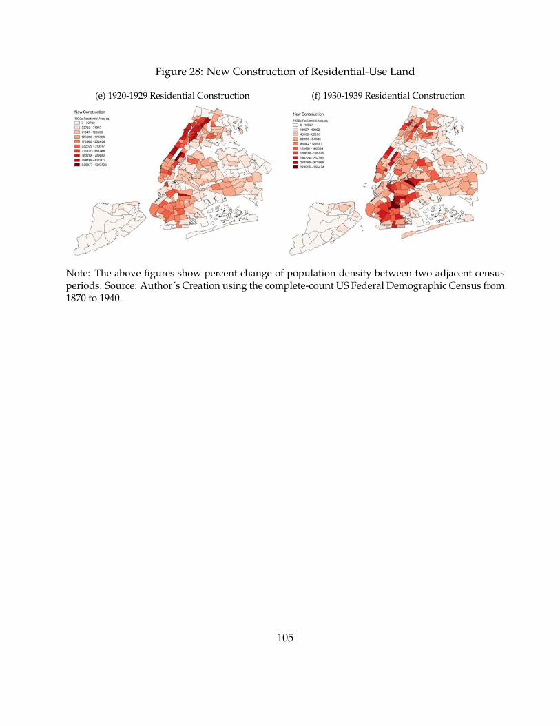
Figure 28: New Construction of Residential-Use Land
(e) 1920-1929 Residential Construction (f) 1930-1939 Residential Construction
Note: The above figures show percent change of population density between two adjacent censusperiods. Source: Author’s Creation using the complete-count US Federal Demographic Census from1870 to 1940.
105
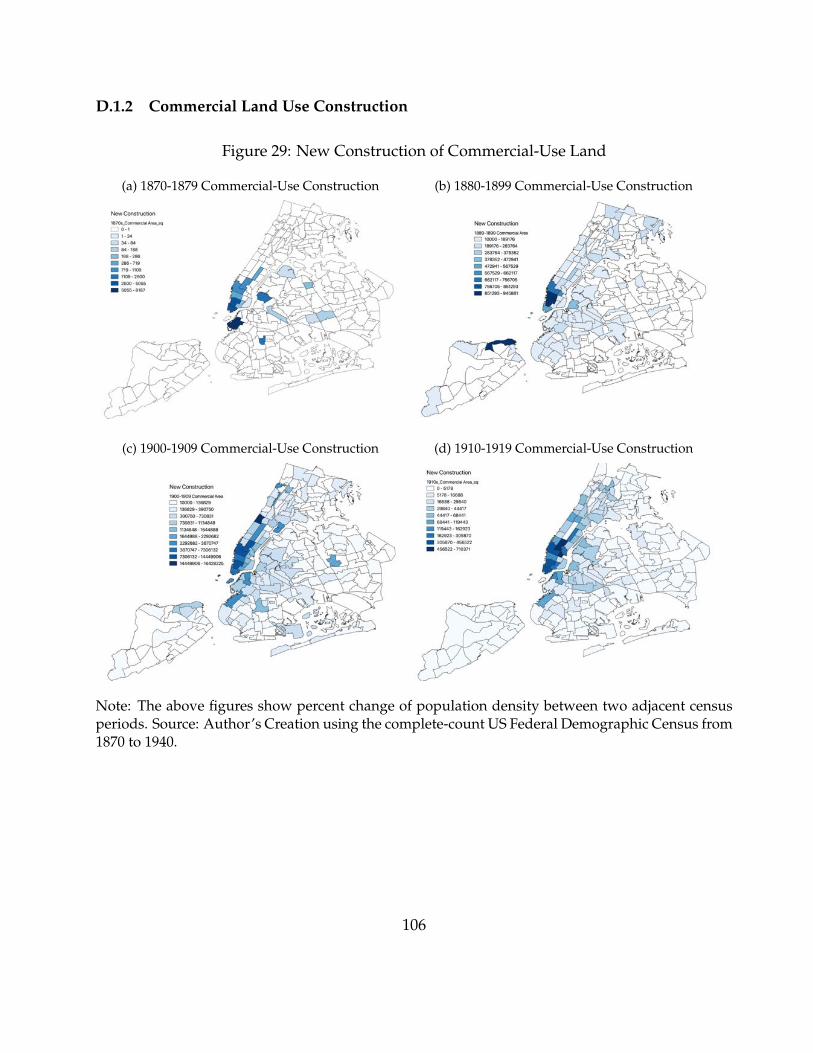
D.1.2 Commercial Land Use Construction
Figure 29: New Construction of Commercial-Use Land
(a) 1870-1879 Commercial-Use Construction (b) 1880-1899 Commercial-Use Construction
(c) 1900-1909 Commercial-Use Construction (d) 1910-1919 Commercial-Use Construction
Note: The above figures show percent change of population density between two adjacent censusperiods. Source: Author’s Creation using the complete-count US Federal Demographic Census from1870 to 1940.
106

Figure 29: New Construction of Commercial-Use Land
(e) 1920-1929 Commercial-Use Construction (f) 1930-1939 Commercial-Use Construction
Note: The above figures show percent change of population density between two adjacent censusperiods. Source: Author’s Creation using the complete-count US Federal Demographic Census from1870 to 1940.
E Theoretical frameworkIn this section, I present the theoretical framework based on Allen and Arkolakis (2015),and Allen et al. (2018). This general equilibrium spatial framework features a dynamicsetting where workers differing in skill and nativity choose where and how to migrate be-tween different locations. This framework allows me to assess the welfare effects of transit-infrastructure driven market access improvement on workers with different nativity andskill in different locations.
E.1 SetupGeography
There is a world comprised of a compact set i 2 {1, ..., N} ⌘ N of locations and inhabitedby workers with different nativity n (foreign-born F, native-born U) and skills s(high skillh and low-skill l), each endowed with a unit of labor which they supply inelastically. LetLn,s
it denote the number of workers in location i of nativity n and skill s. In each locationi 2 N, the four type of workers combine their labor to produce a differentiated variety ofgood using a nested constant elasticity of substitution (CES) production function:
Qi = ( Âs2{h,l}
(( Ân2{F,U}
An,si (Ln,s
i )rs�1)
rs )rs
rs�1 ))r�1
r)
rr�1 (1)
107

where An,si > 0 is the productivity of a worker of nativity n and skill s in location i, rs � 1
is the elasticity of substitution across the nativity of workers of a skill s, and r � 1 is theelasticity of substitution across high-skill and low-skill workers.
Production
Workers in location i with (composite) productivity An,si > 0 earn an (endogenous) wage
wn,si . Product markets are perfectly competitive and a worker in location i of nativity n and
skill sis paid a wage wn,si equal to her marginal product:
wn,si = pi ⇥ (Qi)
1r ⇥ (( Â
n2{F,U}An,s
i (Ln,si )
rs�1rs )
rsrs�1 )(
1rs �
1r ) ⇥ An,s
i ⇥ (Ln,si )�
1rs (2)
, where pi is the equilibrium price of the differentiated variety produced in location i. Underperfect competition and production function above, pitakes the following form:
pi = ( Âs2{h,l}
(( Ân2{F,U}
(An,si )rs(wn,s
i )1�rs)1
1�rs )1�r)1
1�r (3)
where Pi ⌘ (Âj2N(tij pj)1�s)1
1�s is the Dixit-Stiglitz price index, and un,si is a type-specific
amenity for each location.
Trade
As workers have CES preferences over varieties and each location produces a differentiatedvariety, workers will consume varieties produced in other locations. We assume that tradebetween locations is subject to “iceberg” trade costs such that tij � 1 units of a good pro-duced in location i 2 S must be shipped in order for one unit to arrive in location j 2 N ;As a result, the price of a differentiated variety from a location i 2 N and in location j 2 Nis pij = tij pi. Workers have CES preferences over varieties produced in all locations withelasticity of substitution s � 1 and their indirect utility can be written as
Wn,si =
wn,si
Piun,s
i (4)
Given the setup of iceberg trade costs and perfect competition in the production market,gravity trade equation of the value of trade from location i 2 N to location j 2 N , Xij, canbe written as:
Xij = t1�sij (pi)
1�s Ps�1j Ej, (5)
where Ej is the total expenditure in location j.
108
E.2 MigrationE.2.1 Migration decision on which labor market to face
The movement of people across locations are also subject to “iceberg” frictions. For sim-plicity, we take the initial distribution of heterogenous workers with different nativity andskill {Ln,s
i,0 } as exogenous and treat the migration decision as static. Then, a continuum ofheterogenous workers n 2 [0, Ln,s
i,0 ] choose where to live in order to maximizer her welfare:
Un,si (n) = max
j2N⇥
Wn,sj
µn,sij
⇥ #n,sij (n) , (6)
where µn,sij � 1 is a migration friction common to all workers moving from location i 2 N
to location j 2 N of type {n, s}, and #n,sij (n) is a migration friction idiosyncratic to workers
ndrawn from an extreme value (Fréchet) distribution with shape parameter qn,s � 0. Weassume that amenity of a particular place depends on an exogenous term and the localpopulation:
Ln,sij =
⇣µn,s
ij
⌘�qn,s
wn,sj
Pjun,s
j
!qn,s�Pn,s
i��qn,s ⇣
Ln,si,0
⌘, (7)
where�Pn,s
i�=
✓Âj2N
⇣µn,s
ij
⌘�qn,s ⇣Wn,s
j
⌘qn,s◆ 1qn,s
.
Equation 7 is a gravity equation for migration: all else equal, there will be greater flowsfrom location i 2 N to location j 2 N of type {n, s} the lower bilateral migration costs ofworkers with nativity n and skills s, µn,s
ij , the higher type-specific amenity in location j 2 Nfor workers with nativity and skill pair {n, s}, un,s
j , the higher real wages in location j 2 N
for workers with nativity and skill pair {n, s},wn,s
jPj
.
E.2.2 Neighborhood decision and commuting costs
Suppose now that the heterogenous workers with different nativity and skill choose whichneighborhood to live (k 2 K), conditional on working in region j. All neighborhoods k 2 Kare regions such that commuting to location j is feasible, with commuting cost kjk. Underthe Cobb-Douglas preferences, worker preferences are defined over consumption goodsand residential floor space, with the indirect utility for a worker n 2 [0, Ln,s
i,0 ] residing in(k 2 K), working in j is:
Un,sjk (n) = max
k2K⇥
wn,sj un,s
k
kjkPkQk⇥ #n,s
jk (n) , (8)
109

Wn,sj = EKUn,s
jk (n) =
2
4Âk2K
wn,s
j un,sk
kjkPkQk
!Q3
5
1Q
Pk is the price index for consumption goods; Qk is the price of floor space, wn,sj is the
wage of workers with nativity and skill {n, s},kjk is an iceberg commuting cost betweenregion j and neighborhood k 2 K, and commuting costs are same across workers withdifferent nativity and skill, and #n,s
jk (n) is an idiosyncratic amenity draw that captures allthe idiosyncratic factors that cause an individual to live and work in particular locationswithin the city, and #n,s
jk (n) is a commuting friction idiosyncratic to workers ndrawn froman extreme value (Fréchet) distribution with shape parameter Q � 0.
where�Pn,s
i�=
✓Âj2N
⇣µn,s
ij
⌘�qn,s ⇣Wn,s
j
⌘qn,s◆ 1qn,s
.
E.3 EquilibriumGiven a geography of the world, the model elasticities, and the initial distribution of popu-lation {Ln,s
i,0 }, the equilibrium of the model is defined by a set of location observables suchthat:
1. (Law of Motion of Migration) Given wages and the price index, the number of workersof different nativity n (foreign-born F, native-born U) and skills s in each location isequal to the total flows of workers to that location:
Ln,sij =
⇣µn,s
ij
⌘�qn,s
wn,sj
Pjun,s
j
!qn,s�Pn,s
i��qn,s ⇣
Ln,si,0
⌘,
2. Given the number of workers in each location, the quantity of produced of the differ-entiated variety in each location takes the production function from Equation 1
3. (labor market clearing) Given the number of workers in each location, the equilibriumprice and quantity produced of the differentiated variety, the equilibrium wage ofeach type worker with nativity and skill pair {n, s} in each location is equal to itsmarginal product, as in Equation 2
4. (balanced trade) Given the quantity produced of the differentiated variety in each lo-cation, equilibrium prices are determined by the income and expenditure of a locationbeing equal to its total sales:
piQi = Âj2N
t1�qij p1�q
i Ps�1j pjQj
110
Related Documents


![Southern Crabgrass Row Crop [Digitaria ciliaris (Retz ... · Problems Created Southern crabgrass [Digitaria ciliaris (Retz.) Koeler][Digitaria sanguinalis (L.) Scop. var. ciliaris](https://static.cupdf.com/doc/110x72/5b9a56e509d3f2dc2b8d6fc8/southern-crabgrass-row-crop-digitaria-ciliaris-retz-problems-created-southern.jpg)


![Southern Crabgrass Row Crop [Digitaria ciliaris (Retz.) Koeler]](https://static.cupdf.com/doc/110x72/613d6b63736caf36b75d1cd1/southern-crabgrass-row-crop-digitaria-ciliaris-retz-koeler.jpg)