Small Hydro Project Analysis Course No: R03-006 Credit: 3 PDH Velimir Lackovic, Char. Eng. Continuing Education and Development, Inc. 9 Greyridge Farm Court Stony Point, NY 10980 P: (877) 322-5800 F: (877) 322-4774 [email protected]

Welcome message from author
This document is posted to help you gain knowledge. Please leave a comment to let me know what you think about it! Share it to your friends and learn new things together.
Transcript

Small Hydro Project Analysis Course No: R03-006
Credit: 3 PDH
Velimir Lackovic, Char. Eng.
Continuing Education and Development, Inc. 9 Greyridge Farm Court Stony Point, NY 10980 P: (877) 322-5800 F: (877) 322-4774 [email protected]

SMALL HYDRO PROJECT ANALYSIS
This course covers the analysis of potential small hydro projects including a
technology background.
Small Hydro Background
Hydroelectricity is a widely used form of alternative energy, providing more than 19%
of the world’s electric power consumption from both large and small hydro power
plants. Brazil, the United States, Canada and Norway generate large quantities of
electric power from very large hydroelectric facilities. On the other hand, there are
numerous regions of the world that have a huge number of small hydro power plants
in service. For example, in China, more than 19,000 MW of electric power is generated
from 43,000 small hydro power plants.
There is no common definition of the term “small hydro power plant” which, depending
on local interpretations can range from a few kilowatts to 50 megawatts or more of
electric power output. Internationally, “small” hydro power plants usually range in size
from 1 MW to 50 MW. Projects in the 100 kW to 1 MW range are usually referred to
as “mini” hydro plants, and projects under 100 kW in size are referred to as “micro”
hydro power plants. However, installed capacity is not always a proper indicator of the
project size. For instance, a 20 MW, low-head “small” hydro power plant is not small
since low-head hydro facilities usually need and use larger volumes of water, and need
larger hydro turbines in comparison to high-head facilities.
Description of Small Hydro Power Plants
A small hydro power plant can be defined under two main sections: civil works, and
electrical and mechanical equipment.
Civil works
The major civil works of a small hydro power plant construction are the diversion dam
or weir, the water passages and the powerhouse for electrical and mechanical

equipment. The diversion dam or weir directs the water into a canal, tunnel, penstock
or turbine inlet. The water then goes through the turbine, spins it with sufficient force
to generate electric power in a generator. The water then goes back into the river
through a tailrace. In general, small hydro developments built for use at isolated and
remote areas are run-of-river facilities, which mean that water is not kept in a reservoir
and is utilized only as it is available. The price of huge water storage dams cannot
usually be justified for small hydro power plant developments and finally, a low dam
or diversion weir of the simplest construction is usually applied. Dam construction can
be of concrete, wood, masonry or a combination of these materials. Significant effort
continues to be put to decrease the price of dams and weirs for small hydro
developments, as the price of this item alone usually renders a project not
economically viable.
The water passages of a small hydro power plant consist of:
- An intake that includes trashracks, a gate and an entrance to a canal, penstock
or directly to the turbine which depends on the facility type. The intake is
normally constructed of reinforced concrete, the trashrack of steel or iron, and
the gate of wood, iron or steel.
- A canal, tunnel and/or penstock, that transfers the water to the powerhouse in
facilities where the electric and mechanical powerhouse is located at a distance
downstream from the intake. Canals are usually excavated and follow the
contours of the existing terrain. Tunnels are underground and made by drilling
and blasting or by using a tunnel-boring equipment. Penstocks, that convey
water under pressure, can be constructed of steel, iron, fibreglass, plastics,
concrete or wood.
- The entrance and exit of the mechanical turbine that include the valves and
gates required to shut off flow to the turbine for shutdown and maintenance
purposes. These elements are usually made of steel or iron. Gates downstream
of the turbine, if needed for maintenance, can be constructed of wood.
- A tailrace that transfers the water from the turbine exit back to the river. The

tailrace is excavated just like the canal. The turbine or turbines and most of the
electrical and mechanical components are located at the powerhouse. Small
hydro power plants are usually kept to the minimum possible size while still
providing sufficient foundation strength, access for servicing, and safety.
Construction is made of concrete and other local building materials and
components.
Design simplicity, with an emphasis on usability, easily made civil structures is of major
concern for a small hydro power plant project in order to keep prices at a minimum.
Electrical and mechanical equipment
The major mechanical and electrical elements of a small hydro power plant are the
turbine(s) and electrical generator(s). Several different turbines types have been made
to cover the vast range of hydropower site conditions that can be found around the
world. Mechanical turbines that are used for small hydro power developments are
scaled-down versions of conventional large hydro power turbines. Mechanical turbines
that are used for low to medium head developments are typically of the reaction type
and include Francis and fixed and variable pitch (Kaplan) propeller mechanical
turbines. The turbine runner or “wheel” of a reaction turbine is totally submersed in
water. Mechanical turbines utilized for high-head developments are usually referred to
as impulse turbines. These turbines include the Pelton, Turgo and crossflow
arrangements. The impulse turbine runner rotates in the air and is powered by a high-
speed water jet.
Small hydro power turbines can reach efficiencies of around 90%. Care must be taken
when selecting the suitable turbine design for each development as some mechanical
turbines only effectively service over a limited flow range (e.g. propeller mechanical
turbines with fixed blades and Francis mechanical turbines). For many run-of-river
small hydro power sites where water flows significantly change, turbines that function
efficiently over a wide flow range are typically preferred (e.g. Kaplan, Pelton, Turgo
and crossflow designs).
Instead, multiple turbines that work within limited water flow ranges can be utilized.
There are two basic electrical generator types used in small hydro power plants:

induction (asynchronous) or synchronous. A synchronous electrical generator can
function in isolation while an induction generator must typically function in conjunction
with other electrical generators. Synchronous generators are utilized as the primary
power source by electrical utility companies and for isolated diesel-grid and stand-
alone small hydro power developments. Induction electrical generators with capacities
less than about 500 kW are normally best fitted for small hydro power plants delivering
power to a large existing electricity network.
Other electrical and mechanical elements of a small hydro power plant include:
- Speed increaser to match the rotational speed of the mechanical turbine to that
of the electrical generator (if needed)
- Water shut-off valve(s) for the mechanical turbine(s)
- River by-pass gate and checks (if needed)
- Hydraulic control mechanism for the mechanical turbine(s) and valve(s)
- Electrical relay protection and control system
- Electrical switchgear
- Power transformers for station service and electricity transmission
- Station service that includes lighting, heating and power to operate control
systems and electrical switchgear
- Water cooling and lubricating mechanisms (if needed)
- Ventilation mechanisms
- Backup power supply
- Telecommunication mechanism

- Fire and security alarm mechanism (if needed)
- Utility interconnection or transmission and distribution electrical system
Small Hydro Power Project Development
The small hydro power project development usually needs from 2 to 5 years to finish,
from conception to final commissioning. This time is needed to complete studies and
engineering design work, to receive the necessary legal approvals and to construct
the project. Once the small hydro power plant is constructed, it requires insignificant
maintenance over their useful life cycle, which can be more than 50 years. Typically,
one part-time operator can perform control and routine service of a small hydro plant,
with maintenance of the larger and more important elements of a plant normally
needing assistance from outside contractors.
The technical and financial feasibility of each small hydro power development are very
site dependant. Power and energy production depends on the available water (flow)
and head (drop in elevation). Power and energy amount that can be produced
depends on the water quantity and the frequency of flow during the year.
The site economics depends on the energy and power that a development can
generate, whether or not the power can be sold, and the cost paid for the power. In an
isolated area (off-grid and isolated-grid developments) the value of energy produced
for consumption is typically significantly higher than for developments that are
interconnected to a central-grid. However, isolated areas may not be in a position to
use all the available power from the small hydro power plant and, maybe not in a
position to use the power when it is available due to seasonal fluctuations in water flow
and energy usage.
A typical, “rule-of-thumb” relationship is that hydro project power is equal to seven
times the product of the flow (Q) and gross head (H) at the site (P = 7QH). In order to
generate 1 kW of power at a location with 100 m of head, this will need one-tenth the
water flow that a location with 10 m of head would need. The hydro turbine size is
dependent on the water flow it has to accommodate. Thus, the power producing
equipment for higher-head, lower-flow developments is usually less expensive than

for lower-head, higher-flow small hydro power plants.
The same cannot be confirmed for the civil works elements of a small hydro power
project that are related much more to the local topography and physical nature of a
particular location.
Small hydro development types
Small hydro developments can usually be categorised as either “run-of-river
developments” or “water storage developments”.
Run-of-river development type
“Run-of-river” refers to an operation mode in which the hydro power plant uses only
the water that is available in the river natural flow. “Run-of-river” means that there is
no water storage and that power varies with the stream flow.
The power and energy production of run-of-river small hydro power plants changes
with the hydrologic cycle, so they are usually best fitted to provide power to a bigger
electricity system. They do not typically deliver much firm capacity. Therefore, isolated
locations that use small hydro resources usually need auxiliary power. A run-of-river
power plant can only meet all of the electrical requirements of an isolated location or
industry if the minimum water flow in the river is adequate to meet the load’s peak
power needs.
Run-of-river small hydro power plant can call for diversion of the river water flow.
Diversion is usually needed to take advantage of the drop in elevation that occurs over
a distance in the river. Diversion developments decrease the flow in the river between
the intake and the powerhouse. A diversion weir or small dam is usually needed to
divert the flow into the intake.
Water storage (reservoir) developments
For a hydroelectric plant to generate power on demand, either to meet a changing load
or to meet peak power, water must be kept in one or more reservoirs. Unless a natural
lake can be tapped, providing storage typically needs the development of a dam or

dams and the creation of new lakes. This affects the local environment in both negative
and positive directions, even though the scale of project usually amplifies the negative
effects. This usually delivers a conflict, as greater hydro power developments are
appealing since they can deliver “stored” power during peak demand periods. Due to
the economies of scale and the complex approval procedure, storage systems tend to
be relatively big in size.
The development of new storage reservoirs for small hydro power plants is usually not
economically viable except, at remote sites where the energy price is very high.
Storage at a small hydro power plant, if any, is usually limited to small volumes of
water in a new head pond or existing lake upstream of an existing dam. Pondage is
the term applied to define small quantities of water storage. Pondage can offer
advantages to small hydro power plants in the form of increased power generation
and/or enhanced income. Another type of water storage project is “pumped storage”
where water is “recycled” between downstream and upstream storage reservoirs.
Water is directed through mechanical turbines to produce power during peak periods
and pumped back to the upper reservoir during off-peak periods. The feasibility of
pumped storage developments depends on the difference between the values of peak
and off-peak power. Due to the inefficiencies involved in pumping versus producing,
the water recycling leads in net energy consumption. Power used to pump water has
to be produced by other sources.
The environmental effects that can be connected with small hydro power projects can
change significantly depending on the project location and site configuration.
The implications on the environment of constructing a run-of-river small hydro power
plant at an existing dam are usually minor and similar to those related to the expansion
of an existing development. Construction of a run-of-river small hydro power plant at
an undeveloped location can pose extra environmental effects. A small dam or
diversion weir is typically needed. The most feasible project scheme might involve
flooding some rapids upstream of the new small dam or weir.
The environmental effects that can be linked with hydroelectric projects that contain
water storage (typically larger in size) are primarily linked to the creation of a water

storage reservoir. The creation of a reservoir calls for the development of a relatively
big dam, or the use of an existing lake to impound water. The creation of a new
reservoir with a dam involves the flooding of land upstream of the dam. The utilization
of water stored in the reservoir behind a dam or in a lake ends in the changing of water
levels and flows in the river downstream. A rigorous environmental judgement is
usually needed for any development involving water storage.
Hydro project engineering steps
There are usually four steps for engineering work needed to construct a hydro
development. Note, however, that for small hydro power plant, the engineering work
is usually reduced to three steps in order to reduce costs. Typically, initial investigation
is contracted that mixes the necessary work in the first two steps presented below.
The work, however, is finished to a reduced level of detail in order to reduce costs.
While decreasing the engineering work enhances the danger of the development not
being financially feasible, this can normally be justified due to the lower prices linked
with smaller developments.
Reconnaissance surveys and hydraulic assessments
This first step of work usually covers various sites and includes: map assessments;
delineation of the drainage basins; initial approximations of flow and floods; a one day
site visit to each site (by a design engineer and geologist or geotechnical engineer);
initial layout; final grading of locations based on power potential; cost approximations
(based on equations or computer data) and an index of prices.
Pre-feasibility assessment
Development on the selected locations or sites would involve: site mapping and
geological assessments (with drilling confined to locations where foundation
uncertainty would have a critical impact on prices); a reconnaissance for adequate
borrow locations (e.g. for sand and gravel); an initial layout based on materials known
to be available; initial selection of the main development features (installed capacity,
type of construction, etc.); a price assessment based on major amounts; the
identification of potential environmental effects; and production of a single volume

assessment report on each location.
Feasibility assessment
Development would go forward on the selected locations with a major foundation
investigation exercise; delineation and testing of all borrow locations; assessment of
diversion, design and potential maximum floods; determination of energy generating
potential for various dam heights and installed capacities for development
optimisation; determination of the development design earthquake and the maximum
possible earthquake; design of all civil structures in adequate detail to get amounts for
all items that contribute more than about 10% to the price of individual developments;
determination of the dewatering sequence and development plan; optimization of the
development layout, water levels and elements; production of a detailed price
approximation; and eventually, an economic and financial assessment of the
development including an evaluation of the effect on the existing power network along
with a comprehensive assessment study.
System planning and project engineering
This task would involve assessments and final design of the electrical transmission
network; integration of the transmission network; integration of the development into
the electricity grid to check precise servicing mode; preparation of tender drawings
and equipment specifications; assessment of bids and detailed design of the
development; preparation of detailed development drawings and review of
manufacturer’s equipment drawings. However, the limits of this phase would not
involve site supervision nor development management, since this task would form part
of the development execution prices.
Small Hydro Project Modelling
Small hydro power project modelling gives a means to evaluate the available power
at a potential small hydro location that could be delivered to a central-electricity grid
or, for isolated loads, the part of this usable power that could be harnessed by a local
power company (or utilized by the load in an off-grid network). Modelling includes both
run-of-river and reservoir projects, and it integrates advanced rules for calculating

efficiencies of a variety of hydro turbines.
The small hydro power plant model can be utilized to assess small hydro power
developments usually assorted under the following three terms:
- Small hydro
- Mini hydro
- Micro hydro
The small hydro power development model has been made mainly to find out if work
on the small hydro power plant development should continue further or be cancelled
in favor of other options. Each hydro location is specific, since about 75% of the project
cost is defined by the site conditions. Only about 25% of the price is relatively fixed,
being the price of production of the electromechanical parts and elements.
A flowchart of the typical numerical algorithms for small hydro power plant evaluation
is displayed in Figure 1. User inputs involve the flow-duration curve and, for isolated-
electricity network and off-grid purposes, the load-duration curve. Turbine efficiency is
determined at regular intervals on the flow-duration curve. Plant power capacity is then
evaluated and the power-duration curve is made. Usable energy is basically
determined by integrating the power-duration curve. In the case of a central-
transmission network, the energy produced is equal to the energy available. In the
case of an isolated-transmission network or off-grid purpose, the process is slightly
more sophisticated and includes both the power-duration curve and the load-duration
curve.
Figure 1. Small hydro energy model
Flow-duration curve
Calculation of turbine
efficiency curve
Calculation of plant capacity
Calculation of power-
duration curve
Calculation of renewable
energy available
Calculation of renewable
energy delivered
(central grid)
Load-duration curve
Calculation of renewable energy delivered (isolated grid and off-grid)

There are few limitations to formulas shown below. First, the formulas have been made
to assess run-of-river small hydro power developments. The assessment of storage
developments is possible, however, a number of assumptions are needed. Changes
in gross head due to variations in reservoir water level cannot be modelled. The model
needs a unique value for gross head and, in the case of reservoir developments; an
adequate average value must be defined. The determination of the mean head has to
be done outside of the model and will need an understanding of the impacts of
changes in head on annual power generation. Second, for isolated-transmission
network and off-grid applications in isolated locations, the power demand has been
assumed to follow the same pattern for every day of the year. For remote areas where
power requirement and available power change significantly over the course of a year,
modifications will have to be made to the calculated amount of renewable energy
delivered. As will be seen in the next paragraphs, formulas condenses in an easy-to-
use format a wealth of data, and it should be of great help to engineers involved in the
initial assessment of small hydro power developments.
Hydrology
Hydrological information is defined as a flow-duration curve, which is assumed to
represent the flow conditions in the river being suitable over the course of an average
year. For storage developments, information must be defined by the user and should
represent the regulated flow that results from operating a reservoir; at the moment, the
head change with storage drawdown is not included in the model. For run-of-river
developments, the needed flow-duration curve information can be defined either
manually or by using the specific run-off methodology.
A flow-duration curve is a graph of the historical flow at a location ordered from
maximum to minimum flow. The flow-duration curve is used to evaluate the predicted
availability of flow over time, and accordingly the power and energy, at a location. The
model then defines the firm flow that will be usable for electricity generation based on
the flow-duration curve information, the percent time the firm flow should be available,
and the residual flow.
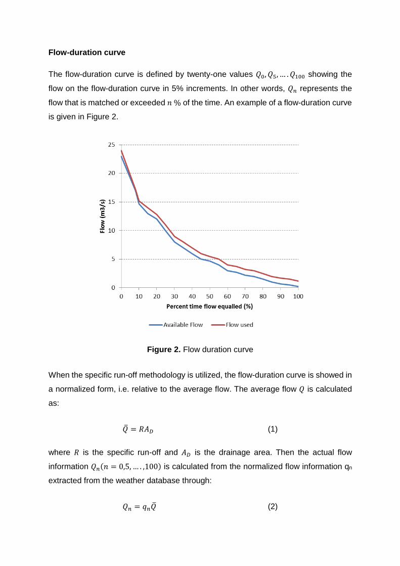
Flow-duration curve
The flow-duration curve is defined by twenty-one values 𝑄𝑄0,𝑄𝑄5, … .𝑄𝑄100 showing the
flow on the flow-duration curve in 5% increments. In other words, 𝑄𝑄𝑛𝑛 represents the
flow that is matched or exceeded 𝑛𝑛 % of the time. An example of a flow-duration curve
is given in Figure 2.
Figure 2. Flow duration curve
When the specific run-off methodology is utilized, the flow-duration curve is showed in
a normalized form, i.e. relative to the average flow. The average flow 𝑄𝑄 is calculated
as:
𝑄𝑄� = 𝑅𝑅𝐴𝐴𝐷𝐷 (1)
where 𝑅𝑅 is the specific run-off and 𝐴𝐴𝐷𝐷 is the drainage area. Then the actual flow
information 𝑄𝑄𝑛𝑛(𝑛𝑛 = 0,5, … . ,100) is calculated from the normalized flow information qn
extracted from the weather database through:
𝑄𝑄𝑛𝑛 = 𝑞𝑞𝑛𝑛𝑄𝑄� (2)

Available flow
Often, a certain quantity of flow must be left in the river throughout the year for
environmental reasons. This residual flow 𝑄𝑄𝑟𝑟 is defined by the user and must be
subtracted from all values of the flow-duration curve for the computation of plant size,
firm capacity and renewable power available, as explained further on in this chapter.
The usable flow 𝑄𝑄𝑛𝑛′ (𝑛𝑛 = 0,5, … . ,100) is then determined by:
𝑄𝑄𝑛𝑛′ = max (𝑄𝑄𝑛𝑛 − 𝑄𝑄𝑟𝑟 , 0) (3) The usable flow-duration curve is displayed in Figure 2, with as an example 𝑄𝑄𝑟𝑟 set to
1 𝑚𝑚3/𝑠𝑠.
Firm flow
The firm flow is determined as the flow being available 𝑝𝑝 % of the time, where 𝑝𝑝 is a
percentage defined by the user and is typically equal to 95%. The firm flow is defined
from the available flow-duration curve. If needed, a linear interpolation between 5%
intervals is used to find the firm flow. In the example of Figure 2 the firm flow is equal
to 1.5 𝑚𝑚3/𝑠𝑠 with p set to 90%.
Load
The degree of sophistication used to define the load depends on the type of
transmission network considered. If the small hydro power plant is interconnected to
a central-grid, then it is assumed that the electricity network absorbs all of the power
production and the load does not need to be defined. If on the other hand the system
is off-grid or interconnected to an isolated-transmission network, then the part of the
power that can be delivered depends on the load. Given methodology assumes that
the daily load requirement is the same for all days of the year and can be represented
by a load-duration curve. An example of such a curve is given in Figure 3. As for the
flow-duration curve given in the previous section, the load-duration curve is defined by
twenty-one values 𝐿𝐿0, 𝐿𝐿5, … . , 𝐿𝐿100 , defining the load on the load-duration curve in 5%
increments; 𝐿𝐿𝑘𝑘 represents the load that is equalled or exceeded 𝑘𝑘 % of the time.

Figure 3. Load duration curve
Energy demand
Daily energy requirement is computed by integrating the area under the load-duration
curve over one day. A simple trapezoidal integration method is used. The daily
requirement 𝐷𝐷𝑑𝑑 expressed in 𝑘𝑘𝑘𝑘ℎ is therefore computed as:
𝐷𝐷𝑑𝑑 = ∑ �𝐿𝐿5(𝑘𝑘−1)+𝐿𝐿5𝑘𝑘2
� 5100
2420𝑘𝑘=1 (4)
with the 𝐿𝐿 expressed in 𝑘𝑘𝑘𝑘. The annual energy requirement 𝐷𝐷 is found by multiplying
the daily requirement by the number of days in a year, 365:
𝐷𝐷 = 365𝐷𝐷𝑑𝑑 (5) Average load factor
The average load factor 𝐿𝐿 is the ratio of the average daily load (𝐷𝐷𝑑𝑑/24) to the peak
load(𝐿𝐿0):
𝐿𝐿� =𝐷𝐷𝑑𝑑24𝐿𝐿0
(6)

This quantity is not utilized by the rest of the algorithm but is simply given to the user
to provide an indication of the variability of the load.
Energy Generation
Given methodology provides estimated alternative energy delivered (MWh) based on
the adjusted available flow (adjusted flow-duration curve), the design flow, the residual
flow, the load (load-duration curve), the gross head and the efficiencies/ losses. The
computation includes a comparison of the daily alternative energy available to the daily
load-duration curve for each of the flow-duration curve figures.
Turbine efficiency curve
Small hydro turbine efficiency information can be defined manually or can be
computed. Computed efficiencies can be adapted using the turbine manufacture/
design coefficient and the efficiency adjustment factor. Standard turbine efficiency
curves have been formulated for the following turbine types:
- Kaplan (reaction turbine)
- Francis (reaction turbine)
- Propellor (reaction turbine)
- Pelton (impulse turbine)
- Turgo (impulse turbine)
- Cross-flow (generally classified as an impulse turbine).
Turbine type is defined based on its suitability to the available head and flow
conditions. The computed turbine efficiency curves take into account a number of
factors including rated head (gross head less maximum hydraulic losses), runner
diameter, turbine specific speed and the turbine manufacture/design coefficient. The
efficiency formulas were deducted from a large number of manufacture efficiency
curves for different turbine models and head and flow conditions.

For various turbine applications it is assumed that all turbines are the same and that
a single turbine will be utilized up to its maximum flow and then flow will be divided
equally between two turbines, and so on up to the maximum number of turbines
selected. The turbine efficiency formulas and the number of turbines are utilized to
compute plant turbine efficiency from 0% to 100% of design flow (maximum plant flow)
at 5% intervals. An example turbine efficiency curve is given in Figure 4 for 1 and 2
turbines.
Figure 4. Computed efficiency curves for Francis turbine
Power available as a function of flow
Actual power 𝑃𝑃 usable from the small hydro power plant at any given flow value 𝑄𝑄 is
defined by the following formula, in which the flow-dependent hydraulic losses and
tailrace reduction are taken into account:
𝑃𝑃 = 𝜌𝜌𝜌𝜌𝑄𝑄�𝐻𝐻𝑔𝑔 − �ℎℎ𝑦𝑦𝑑𝑑𝑟𝑟 + ℎ𝑡𝑡𝑡𝑡𝑡𝑡𝑡𝑡��𝑒𝑒𝑡𝑡𝑒𝑒𝑔𝑔(1 − 𝑙𝑙𝑡𝑡𝑟𝑟𝑡𝑡𝑛𝑛𝑡𝑡)�1 − 𝑙𝑙𝑝𝑝𝑡𝑡𝑟𝑟𝑡𝑡� (7)
where 𝜌𝜌 is the density of water (1,000 kg/m3), 𝜌𝜌 the acceleration of gravity (9.81 m/s2),

𝐻𝐻𝑔𝑔 the gross head, ℎℎ𝑦𝑦𝑑𝑑𝑟𝑟 and ℎ𝑡𝑡𝑡𝑡𝑡𝑡𝑡𝑡 are respectively the hydraulic losses and tailrace
effect associated with the flow; and 𝑒𝑒𝑡𝑡 is the turbine efficiency at flow 𝑄𝑄. Finally, 𝑒𝑒𝑔𝑔 is
the generator efficiency, 𝑙𝑙𝑡𝑡𝑟𝑟𝑡𝑡𝑛𝑛𝑡𝑡 the transformer losses, and 𝑙𝑙𝑝𝑝𝑡𝑡𝑟𝑟𝑡𝑡 the parasitic electricity
losses 𝑒𝑒𝑔𝑔. 𝑙𝑙𝑡𝑡𝑟𝑟𝑡𝑡𝑛𝑛𝑡𝑡, and 𝑙𝑙𝑝𝑝𝑡𝑡𝑟𝑟𝑡𝑡 are determined by the user and are assumed independent
from the considered flow. Hydraulic losses are adapted over the range of available
flows based on the following formula:
ℎℎ𝑦𝑦𝑑𝑑𝑟𝑟 = 𝐻𝐻𝑔𝑔𝑙𝑙ℎ𝑦𝑦𝑑𝑑𝑟𝑟,𝑚𝑚𝑡𝑡𝑚𝑚𝑄𝑄2
𝑄𝑄𝑑𝑑𝑑𝑑𝑑𝑑2 (8)
where 𝑙𝑙ℎ𝑦𝑦𝑑𝑑𝑟𝑟,𝑚𝑚𝑡𝑡𝑚𝑚 is the maximum hydraulic losses defined by the user, and 𝑄𝑄𝑑𝑑𝑑𝑑𝑡𝑡 the
design flow. Similarly the maximum tailrace effect is adapted over the range of
available flows with the following formula:
ℎ𝑡𝑡𝑡𝑡𝑡𝑡𝑡𝑡 = ℎ𝑡𝑡𝑡𝑡𝑡𝑡𝑡𝑡,𝑚𝑚𝑡𝑡𝑚𝑚(𝑄𝑄−𝑄𝑄𝑑𝑑𝑑𝑑𝑑𝑑)2
(𝑄𝑄𝑚𝑚𝑚𝑚𝑚𝑚−𝑄𝑄𝑑𝑑𝑑𝑑𝑑𝑑)2 (9)
where ℎ𝑡𝑡𝑡𝑡𝑡𝑡𝑡𝑡,𝑚𝑚𝑡𝑡𝑚𝑚 is the maximum tailwater impact, i.e. the maximum decrease in
available gross head that will occur during times of high flows in the river. 𝑄𝑄𝑚𝑚𝑡𝑡𝑚𝑚 is the
maximum river flow, and equation (9) is used only to river flows that are higher than
the plant design flow (i.e. when 𝑄𝑄 > 𝑄𝑄𝑑𝑑𝑑𝑑𝑡𝑡).
Plant capacity
Plant capacity 𝑃𝑃𝑑𝑑𝑑𝑑𝑡𝑡 is determined by re-writing formula (7) at the design flow 𝑄𝑄𝑑𝑑𝑑𝑑𝑡𝑡 .
The formula simplifies to:
𝑃𝑃𝑑𝑑𝑑𝑑𝑡𝑡 = 𝜌𝜌𝜌𝜌𝑄𝑄𝑑𝑑𝑑𝑑𝑡𝑡𝐻𝐻𝑔𝑔(1 − 𝑙𝑙ℎ𝑦𝑦𝑑𝑑𝑟𝑟)𝑒𝑒𝑡𝑡,𝑑𝑑𝑑𝑑𝑡𝑡𝑒𝑒𝑔𝑔(1 − 𝑙𝑙𝑡𝑡𝑟𝑟𝑡𝑡𝑛𝑛𝑡𝑡)(1− 𝑙𝑙𝑝𝑝𝑡𝑡𝑟𝑟𝑡𝑡) (10)
where 𝑃𝑃𝑑𝑑𝑑𝑑𝑡𝑡 is the plant capacity and 𝑒𝑒𝑡𝑡,𝑑𝑑𝑑𝑑𝑡𝑡 the turbine efficiency at design flow.
The small hydro plant firm capacity is defined again with formula (7), but this time using
the firm flow and corresponding turbine efficiency and hydraulic losses at this flow. If
the firm flow is higher than the design flow, firm plant capacity is set to the plant
capacity computed through formula (10).

Power-duration curve
Computation of power usable as a function of flow, using formula (7) for all 21 values
of the available flow 𝑄𝑄0′ ,𝑄𝑄5′ , … . . ,𝑄𝑄100′ used to define the flow-duration curve, leads to
21 values of available power 𝑃𝑃0,𝑃𝑃1, … . . ,𝑃𝑃100 , defining a power-duration curve. Since
the design flow is defined as the maximum flow that can be utilized by the turbine, the
flow values utilized in formulas (7) and (8) are actually 𝑄𝑄𝑛𝑛,𝑢𝑢𝑡𝑡𝑑𝑑𝑑𝑑 determined as:
𝑄𝑄𝑛𝑛,𝑢𝑢𝑡𝑡𝑑𝑑𝑑𝑑 = min (𝑄𝑄𝑛𝑛′ ,𝑄𝑄𝑑𝑑𝑑𝑑𝑡𝑡) (11)
An example power-duration curve is given in Figure 5, with the design flow equal to 3
m3/s.
Figure 5. Power duration curve
Renewable energy available
Renewable energy available is defined by computing the area under the power curve
assuming a straight-line between adjacent computed power output figures. Provided
that the flow-duration curve represents an annual cycle, each 5% interval on the curve

is equal to 5% of 8,760 hours (number of hours per year). The annual available energy
𝐸𝐸𝑡𝑡𝑎𝑎𝑡𝑡𝑡𝑡𝑡𝑡 (in kWh/yr) is therefore computed from the values P (in kW) by:
𝐸𝐸𝑡𝑡𝑎𝑎𝑡𝑡𝑡𝑡𝑡𝑡 = ∑ �𝑃𝑃5(𝑘𝑘−1)+𝑃𝑃5𝑘𝑘2
� 5100
8760(1 − 𝑙𝑙𝑑𝑑𝑡𝑡)20𝑘𝑘=1 (12)
where 𝑙𝑙𝑑𝑑𝑡𝑡 is the annual downtime losses as defined by the user. In the case where the
design flow falls between two 5% increments on the flow-duration curve the interval is
divided in two, and a linear interpolation is utilized on each side of the design flow.
Equation (12) determines the quantity of renewable energy available. The quantity
actually delivered depends on the type of transmission network, as is presented in the
following paragraphs.
Renewable energy delivered - central-grid
For central-grid use, it is assumed that the electricity grid is able to absorb all the
energy generated by the small hydro power plant. Therefore, all the alternative energy
available will be provided to the central-electricity grid and the renewable energy
provided, 𝐸𝐸𝑑𝑑𝑡𝑡𝑎𝑎𝑑𝑑, is simply:
𝐸𝐸𝑑𝑑𝑡𝑡𝑎𝑎𝑑𝑑 = 𝐸𝐸𝑡𝑡𝑎𝑎𝑡𝑡𝑡𝑡𝑡𝑡 (13) Renewable energy delivered - isolated-grid and off-grid
For isolated-electricity grid and off-grid developments the process is slightly more
complex because the energy delivered is actually limited by the needs of the local
electricity network or the load, as defined by the load-duration curve (Figure 3). The
following process is utilized: for each 5% increase on the flow-duration curve, the
corresponding available plant power production (assumed to be same over a day) is
compared to the load-duration curve (assumed to represent the daily load
requirement). The part of energy that can be provided by the small hydro power plant
is defined as the area that is under both the load-duration curve and the horizontal line
representing the available plant power generation. Twenty-one figures of the daily
energy provided 𝐺𝐺0,𝐺𝐺1, … . . ,𝐺𝐺100 corresponding to the available power 𝑃𝑃0,𝑃𝑃1, … . . ,𝑃𝑃100
are computed. For each figure of usable power 𝑃𝑃𝑛𝑛, the daily energy provided 𝐺𝐺𝑛𝑛, is
defined by:

𝐺𝐺𝑛𝑛 = ∑ �𝑃𝑃𝑛𝑛,5(𝑘𝑘−1)′ +𝑃𝑃𝑛𝑛,5𝑘𝑘
′
2� 5100
2420𝑘𝑘=1 (14)
where 𝑃𝑃𝑛𝑛,𝑘𝑘′ is the lesser of load 𝐿𝐿𝑘𝑘 and usable power 𝑃𝑃𝑛𝑛 :
𝑃𝑃𝑛𝑛,𝑘𝑘′ = min (𝑃𝑃𝑛𝑛,𝐿𝐿𝑘𝑘) (15)
In the case where the available power 𝑃𝑃𝑛𝑛,𝑘𝑘
′ falls between two 5% increments on the
load duration curve, the interval is split in two and a linear interpolation is used on each
side of the available power.
This process is explained by an example, using the load-duration curve from Figure 3
and figures from the power-duration curve given in Figure 5. The aim of the example
is to define the daily alternative energy 𝐺𝐺75 provided for a flow that is exceeded 75%
of the time. Reference to Figure 5 should be made to define the corresponding power
level:
𝑃𝑃75 = 2,630 𝑘𝑘𝑘𝑘 (16)
Then the resulting value should be reported as a horizontal line on the load-duration
curve, as given in Figure 6. The area that is both under the load-duration curve and
the horizontal line is the alternative energy provided per day for the plant capacity that
matches to flow 𝑄𝑄75. Integration with equation (14) provides the result:
𝐺𝐺75 = 56.6 𝑀𝑀𝑘𝑘ℎ/𝑑𝑑 (17)

Figure 6. Calculation of daily renewable energy delivered
This process is repeated for all values 𝑃𝑃0,𝑃𝑃1, … . . ,𝑃𝑃100 to find twenty one values of the
daily alternative energy provided 𝐺𝐺0,𝐺𝐺1, … . . ,𝐺𝐺100, as a function of percent time the flow
is exceeded as given in Figure 7. The annual alternative energy provided, 𝐸𝐸𝑑𝑑𝑡𝑡𝑎𝑎𝑑𝑑, is
found simply by computing the area under the curve of Figure 7, again with a
trapezoidal rule:
𝐸𝐸𝑑𝑑𝑡𝑡𝑎𝑎𝑑𝑑 = ∑ �𝐺𝐺5(𝑛𝑛−1)+𝐺𝐺5𝑛𝑛2
� 5100
365(1 − 𝑙𝑙𝑑𝑑𝑡𝑡)20𝑘𝑘=1 (18)
where, as before, 𝑙𝑙𝑑𝑑𝑡𝑡 is the annual downtime losses as defined by the user.

Figure 7. Calculation of annual renewable energy delivered
Small hydro plant capacity factor
The annual capacity factor K of the small hydro power plant is a measure of the
available flow at the location and how efficiently it is utilized. It is determined as the
average output of the plant in comparison to its rated capacity:
𝐾𝐾 = 𝐸𝐸𝑑𝑑𝑑𝑑𝑑𝑑𝑑𝑑8760𝑃𝑃𝑑𝑑𝑑𝑑𝑑𝑑
(19)
where the annual alternative energy provided, 𝐸𝐸𝑑𝑑𝑡𝑡𝑎𝑎𝑑𝑑, computed through (13) or (18) is
defined in kWh, and plant capacity computed through (10) is shown in kW.
Excess renewable energy available
Excess renewable energy available 𝐸𝐸𝑑𝑑𝑚𝑚𝑒𝑒𝑑𝑑𝑡𝑡𝑡𝑡, is the difference between the alternative
energy available 𝐸𝐸𝑡𝑡𝑎𝑎𝑡𝑡𝑡𝑡𝑡𝑡, and the alternative energy provided 𝐸𝐸𝑑𝑑𝑡𝑡𝑎𝑎𝑑𝑑:
𝐸𝐸𝑑𝑑𝑚𝑚𝑒𝑒𝑑𝑑𝑡𝑡𝑡𝑡 = 𝐸𝐸𝑡𝑡𝑎𝑎𝑡𝑡𝑡𝑡𝑡𝑡 − 𝐸𝐸𝑑𝑑𝑡𝑡𝑎𝑎𝑑𝑑 (20)
𝐸𝐸𝑡𝑡𝑎𝑎𝑡𝑡𝑡𝑡𝑡𝑡 is computed through formula (12) and 𝐸𝐸𝑑𝑑𝑡𝑡𝑎𝑎𝑑𝑑 through either (13) or (18).

Summary
In this course, the computation method for small hydro power plant technical
parameters has been presented in detail. Generic formulae enable the computation of
turbine efficiency for a variety of turbines. These efficiencies, together with the flow-
duration curve and (in the case of isolated-transmission network and off-transmission
network developments) the load-duration curve, enable the computation of alternative
energy provided by a proposed small hydro power plant. The condensed calculations
enable the evaluation of development costs; alternatively, a detailed pricing
methodology can be utilized. The process illustrated above is excellent for pre-
feasibility stage assessments related to small hydro developments.

References: Clean Energy Project Analysis RETScreen® Engineering & Cases Textbook, Third Edition, © Minister of Natural Resources Canada 2001-2005, September 2005
Related Documents