Coupling level set/VOF/ghost ﬂuid methods: Validation and ...frey/papers/Navier-Stokes/Menard T... · The level set–VOF coupling is validated on 2D and 3D test cases. ... handle

International Journal of Multiphase Flow 33 (2007) 510–524

www.elsevier.com/locate/ijmulflow

Coupling level set/VOF/ghost fluid methods: Validationand application to 3D simulation of the primary

break-up of a liquid jet

T. Menard a, S. Tanguy b, A. Berlemont a,*

a UMR6614-CORIA, Technopole du Madrillet, BP 12 Avenue de l’Universite, 76801 Saint-Etienne-du-Rouvray Cedex, Franceb LEMTA CNRS UMR – 7563, 2, avenue de la foret de Haye, BP 160, 54504 Vandoeuvre les Nancy, France

Received 9 March 2006; received in revised form 23 October 2006

Abstract

Numerical simulations are carried out to describe the dense zone of a spray where very little information is available,either from experimental or theoretical approaches. Interface tracking is ensured by the level set method and the ghost fluidmethod (GFM) is used to capture accurately sharp discontinuities for pressure, density and viscosity. The level set methodis coupled with the VOF method for mass conservation.

The level set–VOF coupling is validated on 2D and 3D test cases. The level set–ghost fluid method is applied to theRayleigh instability of a liquid jet. Preliminary results are then presented for 3D simulation of the primary break-up ofa turbulent liquid jet with the level set–VOF–ghost fluid method.� 2006 Published by Elsevier Ltd.

1. Introduction

Extensive studies have been devoted to the transport of droplet sprays, but the atomization process remainsa challenging topic of research; DNS simulations provide a promising tool for obtaining information in thedense zone of the spray, where nearly no experimental data are available. But it clearly appears that specificapproaches must be developed for the description of interface behavior. Computing interface motion in mul-tiphase flows is a wide field of research and several approaches can be used. Front tracking methods (Unverdiand Tryggvason, 1992), Volume of fluid methods (Gueyffier et al., 1999) and level set methods (Sussman et al.,1994) are the most common numerical strategies used to predict interface motion. Front tracking methods arebased on the Lagrangian tracking of marker particles that are attached to the interface motion, but appearnumerically limited for 3D geometries, especially for the distribution of the marker particles when irregular-ities occur on the interface. Volume of fluid methods are based on the description of the volumetric fraction ofeach phase in grid cells. The main difficulty of the method is that 2D interface reconstruction is quite difficult,

0301-9322/$ - see front matter � 2006 Published by Elsevier Ltd.

doi:10.1016/j.ijmultiphaseflow.2006.11.001

* Corresponding author. Tel.: +33 2 32 95 36 17; fax: +33 2 32 91 04 85.E-mail address: [email protected] (A. Berlemont).

mailto:[email protected]

T. Menard et al. / International Journal of Multiphase Flow 33 (2007) 510–524 511

and 3D reconstruction is numerically prohibitive. A consequence can be some uncertainties on the interfacecurvature and thus on the surface tension forces. The basis of the Level Set methods has been proposed byOsher and Sethian (1988); the interface is described with the zero level curve of a continuous function definedby the signed distance to the interface. To ensure that the function remains the signed distance to the interface,a redistancing algorithm is applied, but it is well known that its numerical computation can generate mass lossin under-resolved regions. This is the main drawback of level set methods. To describe the interface discon-tinuities, two approaches can be used, namely the continuous force formulation (‘‘delta’’ formulation), whichassumes that the interface is 2 or 3 grid meshes thick, and the ghost fluid method (GFM), which has beenderived by Fedkiw et al. (1999) to capture jump conditions on the interface. The GFM approach not onlyavoids the introduction of a fictitious interface thickness, but it is also suitable to provide a more accuratediscretization of discontinuous terms, reducing parasitic currents and improving the resolution on the pressurejump condition (Kang et al., 2000; Tanguy and Berlemont, 2005).

We are here concerned by the primary break-up of a jet and many topological changes occur (interfacepinching or merging, droplet coalescence or secondary break-up). The numerical method must describe theinterface motion precisely, handle jump conditions at the interface without artificial smoothing, and respectmass conservation. Thus we develop a 3D code, where interface tracking is performed by a level set method,the ghost fluid method is used to capture accurately sharp discontinuities, and the level set and VOF methodsare coupled to ensure mass conservation (Sussman and Puckett, 2000). A projection method is used to solveincompressible Navier–Stokes equations that are coupled to a transport equation for the level set function.Specific care has been devoted to improving simulation capabilities with MPI parallelization. We first recallthe level set method, then describe the coupling between the level set and VOF techniques and we briefly pres-ent the ghost fluid method. Validation test cases are performed and discussed and results are then presentedfor the primary break-up of a liquid jet with initial turbulent perturbation on the inflow conditions in order toillustrate the potentialities of the method.

2. Methods

2.1. Level set

Level set methods are based on the use of a continuous function / to describe the interface between twomedia (Sethian, 1996; Osher and Fedkiw, 2003). That function is defined as the signed distance betweenany point of the domain and the interface which is thus described by the 0 level curve of that function. Solvinga convection equation determines the evolution of the interface in a given velocity field ~V:

o/otþ ~V � r/ ¼ 0 ð1Þ

Specific care is taken with the discretization method, as discontinuities are often observed in the results. Toavoid singularities in the distance function field, we thus use the 5th-order WENO scheme for convectiveterms.

Geometrical information on the interface, such as normal vector ~N or curvature j, is easily obtainedthrough:

~N ¼ r/jr/j jð/Þ ¼ �r � ~N ð2Þ

Some problems may arise when the level set method is carried out; high velocity gradients can produce widespreading and stretching of the level set, and / will no longer remain a distance function. A redistancing algo-rithm (Sussman et al., 1998) is thus applied to keep / as the signed distance to the interface. The algorithm isbased on the iterative resolution of the following equation:

odos¼ signð/Þð1� jr/jÞ where dðx; t; sÞs¼0 ¼ /ðx; tÞ ð3Þ

512 T. Menard et al. / International Journal of Multiphase Flow 33 (2007) 510–524

where s is a fictitious time. We solve Eq. (3) until a steady state is reached, thus close to the exact steady statesolution, namely either sign(/) = 0, meaning that we are on the droplet interface, or jrdj ¼ 1 which mathe-matically defines a distance function. We then replace /ðx; tÞ by d(x, t,ssteady).

Numerical computation of Eqs. (1) and (3) can induce mass loss in under-resolved regions. This is the maindrawback of level set methods, but to improve mass conservation, two main extensions of the method can bedeveloped: the particle level set (Enright et al., 2002) and a coupling between VOF and level set (Sussman andPuckett, 2000; van der Pijl et al., 2005). In jet atomization, the interface becomes very wrinkled and manybreak-ups are initiated. It thus appears that coupling the level set method with the VOF technique is muchbetter adapted for our purpose than the particle level set method, and it is presented in next section.

2.2. Coupling VOF and level set methods

As mentioned above, mass conservation in level set methods requires the mesh to be refined enough toavoid under-resolved region as much as possible. That is unrealistic in 3D configurations and different strat-egies have been proposed to overcome this difficulty. Most of them are based on the modification of the reini-tialization algorithm by adding a constraint to help in mass conservation (Sussman et al., 1998). A majorlimitation of these methods is that they are global; when many liquid parcels are generated in the flow thesecorrections are quite impossible.

We thus chose to use the Bourlioux (1995) and Sussman and Puckett (2000) approach (CLSVOF). Themain idea is to benefit from the advantage of each strategy, which is to minimize mass loss through theVOF method and to keep a fine description of the geometrical properties of the interface with the level setmethod. We recall here the main ideas of the CLSVOF method extensively discussed by Sussman and Puckett(2000) and we describe our numerical technique that retains the original CLSVOF method, but we alsokeep the redistancing algorithm for the level set. In addition the calculation of the liquid volume fraction isdetailed.

To couple the VOF method and the level set method, Sussman and Puckett (2000) first defined the volumefraction F, in a grid cell X of the domain, at time t, as a function of the level set / (assuming 2D formalism forsimplicity):

F ðX; tÞ ¼ 1

jXj

ZX

HðUðx; y; tÞdxdy ð4Þ

where H is the Heaviside function: HðUÞ ¼1 if U > 0

0 otherwise

(ð5Þ

It is impossible to transport the liquid volume fraction on the computational domain without knowing theinterface position. But using the level set, the interface can be localized and the liquid volume fraction canbe advected without any ambiguity.

2.2.1. How to get the volume fraction with the level set

To transport the liquid volume fraction or to define it from the Level Set function, we first define the inter-face in the cell Xi;j as a straight line in 2D (a plane in 3D). A reconstructed level set UR

i;j is defined by Sussmanand Puckett (2000):

URi;j ¼ ai;jðx� xiÞ þ bi;jðy � yjÞ þ ci;j ð6Þ

When that equation is normalized such that ða2i;j þ b2

i;jÞ ¼ 1, then ai;j and bi;j are the coordinates of the vectornormal to the interface. Thus the coefficients ci;j represent the normal distance from the interface to the pointsðxi; yjÞ.

The coefficients ai,j, bi,j, ci,j are determined so that URi;j is as close as possible to the real value of the level set

function /. The following error is thus minimized (Sussman and Puckett, 2000):

Ei;j ¼Z xiþ1=2

xi�1=2

Z yjþ1=2

yj�1=2

dðUÞðU� ai;jðx� xiÞ � bi;jðy � yjÞ � ci;jÞ2 dxdy ð7Þ


Using a nine point stencil, discretization of Eq. (7) reads:

Ei;j ¼Xi0¼iþ1

i0¼i�1

Xj0¼jþ1

j0¼j�1

wi0�i;j0�jdeðUi0;j0 ÞðUi0 ;j0 � ai;jðxi0 � xiÞ � bi;jðyj0 � yjÞ � ci;jÞ2 ð8Þ

deðUi0;j0 Þ is a smoothed Dirac distribution with thickness e ðe ¼ffiffiffi2p

dxÞ and wp;q are weighting factors that aremaximal on the cell central point ði; jÞ. Minimizing Ei;j leads to the following conditions:

oEi;j

oai;j¼ oEi;j

obi;j¼ oEi;j

oci;j¼ 0 ð9Þ

Eq. (9) requires solving the following 3 · 3 linear system (4 · 4 in 3D):
PPwhX 2 PP
whXYPP

whXPPwhXY

PPwhY 2 PP

whYPPwhX

PPwhY

PPwh

264375 ai;j

bi;j

ci;j

264375 ¼

PPwhUXPPwhUYPPwhU

264375 ð10Þ

where the following notations are used:
XX$Xi0¼iþ1
i0¼i�1

Xj0¼jþ1

j0¼j�1

wh$ wi0�i;j0�jdeðUi0;j0 ÞX $ ðxi0 � xiÞY $ ðyj0 � yjÞU$ Ui;j

ð11Þ

A classical linear algorithm can be used to obtain the coefficients ai;j; bi;j; ci;j.Defining the zero level set in a cell allows the initial liquid volume fraction F ðXi;j; t ¼ 0Þ to be determined:

F i;j ¼1

dxdy

Z xiþ1=2

xi�1=2

Z yjþ1=2

yj�1=2

Hðai;jðx� xiÞ þ bi;jðy � yjÞ þ ci;jÞdxdy ð12Þ

Eq. (12) can be easily estimated with geometrical relations; for example in Fig. 1, it corresponds to the sum ofthe trapeze area A1 and the rectangle area A2.

Note that in 3D configurations, geometrical relations are a little more complicated. We thus set up amethod that calculates the liquid volume fraction by integrating the line equation (or the plane equation in3D).

Writing the line equation aX þ bY þ c ¼ 0 as Y ¼ AX þ B;R

Y (normalised by S = dxdy) can be analyti-cally calculated. However, the origin of the coordinate system must be defined first; we choose the point withthe smallest coordinates, namely ðxi�1=2, yj�1=2Þ. We might then modify the signs of the coefficients a0i;j and b0i;j,

Fig. 1. VOF geometrical scheme.


such that the normal vector to the interface points towards that origin, to ensure that the calculated volume isthe liquid volume. Finally we determine the new coefficient c0i;j in order to obtain the line equationa0ðx� xi�1=2Þþ b0ðy � yj�1=2Þþc0 ¼ 0. The integral limits are thus the intersection points between the line andthe edges of the cell. The scheme is thus:

ai;jðx� xiÞ þ bi;jðy � yjÞ þ ci;j ¼ 0 becomes

a0i;jðx� xi�1=2Þ þ b0i;jðy � yj�1=2Þ þ c0i;j ¼ 0

with

a0i;j ¼ �ai;j if ai;j > 0

b0i;j ¼ �bi;j if bi;j > 0

c0i;j ¼ ci;j � ða0i;j0:5dxþ b0i;j0:5dyÞ

8>>>>>>>>>>><>>>>>>>>>>>:ð13Þ

Going back to the case in Fig. 1, we get (Fig. 2)

F i;j ¼1

dxdyAX 2 þ BX� �X 1

X 0þ X 0 dy

� �with A ¼

�a0i;jb0i;j

and B ¼�c0i;jb0i;jðbi;j 6¼ 0Þ ð14Þ

If ai;j or bi;j is equal to zero, the line is parallel to one of the axes and no integration is required. This methodhas been extended to 3D configuration and proves much less difficult to set up than the geometrical approach.

2.2.2. How to correct the level set with the volume fraction

The inverted problem can also be solved, that is the correction of the level set when the liquid volume frac-tion is known. For any time n, the volume of liquid in a cell must be the same, whatever the method used forits calculation, either from the level set position or from the result of the transport equation for the liquid vol-ume fraction. For a given volume fraction F n

i;j, we can write (Sussman and Puckett, 2000)):

1

dxdy

Z yjþ1=2

yj�1=2

Z xiþ1=2

xi�1=2

Hðai;jðx� xiÞ þ bi;jðy � yjÞ þ ci;jÞdxdy ¼ F ni;j ð15Þ

where the coefficients ai;j; bi;j; ci;j are given by the zero level set position Un;Ri;j at time n. If the equality is not

satisfied, a Newton iterative method is applied on the coefficient ci;j (no change on the vector normal to theinterface) until a given precision is satisfied for Eq. (15):

cNEWi;j ¼ ci;j �

1dx dy

R yjþ1=2

yj�1=2

R xiþ1=2

xi�1=2ðHðai;jðx� xiÞ þ bi;jðy � yjÞ þ ci;jÞdxdyÞ � F n

i;j

� �R yjþ1=2

yj�1=2

R xiþ1=2

xi�1=2dðai;jðx� xiÞ þ bi;jðy � yjÞ þ ci;jÞdxdy

dxdy ð16Þ

Note that the denominator in Eq. (16) is equal to the length of the zero level set line in the cell (area of theplane in 3D).

gas

xi-1/2,j-1/2

dx

dy

x1x00

A0

Fig. 2. Change of coordinate system for VOF.


2.3. Coupling the transport of the volume fraction and the level set

The liquid volume fraction is a passive scalar; thus its transport equation is similar to the transportequation (Eq. (1)) of the level set. That equation is discretized following the scheme as defined by Sussmanand Puckett (2000); details on the coupled second-order conservative operator split advection are notrecalled here. Nevertheless it is important to note that the advection of the liquid volume fraction is carriedout with the aid of the zero level set in cells where the interface occurs. The overall algorithm used is nowdescribed:

2.3.1. Initialization

Start from a given Un¼0

• Calculate ai;j; bi;j; ci;j and UR;n¼0i;j :

• Calculate F n¼0i;j (Eq. (12)).

1. Coupled advection of F and U
• Set U ¼ Un:• Get ~F n and eU with convection of Fn and / in x or y direction (alternately swapped).• Calculate ai;j; bi;j; ci;j for eUR
i;j:• Calculate cnew

i;j (Eq. (16)) and ~URi;j for mass conservation.

• Get F n and U with convection of ~F n and eU in y or x direction (alternately swapped)• Get F nþ1 and Unþ1 following the operator split algorithm (Sussman and Puckett, 2000).• Correction of F nþ1by setting

F nþ1 ¼ 0 if F nþ1 < 0 or Unþ1 < �Dx

F nþ1 ¼ 1 if F nþ1 > 1 or Unþ1 > Dx

F nþ1 ¼ F nþ1 otherwise

to avoid jetsam or flotsam from the VOF transport.• Calculate ai;j; bi;j; ci;j and correction of Unþ1:• Get final Unþ1 with the redistancing algorithm, applied for F nþ1 ¼ 0 or F nþ1 ¼ 1 thus no change on the

zero level set.
2. Navier–Stokes equation
• Projection method and then go back to step 1.

2.4. Projection method

The joint level set/VOF method is coupled with a projection method for the direct numerical simulation ofincompressible Navier–Stokes equations, expressed as follows:

o~V

otþ ð~V � rÞ~V ¼ �rp

qþr � ð2lDÞ

qþ g

r � ~V ¼ 0

ð17Þ

where p is the fluid pressure, g the gravity vector, l the dynamic viscosity and D is the viscous deformationtensor:

D ¼ 1=2ðrVþrVTÞ ð18Þ
In the projection method, the velocity components are expressed on a staggered grid. Spatial derivatives areestimated with a 2nd-order central scheme, but convective terms are approximated by 5th-order WENOscheme discretization in order to ensure a robust behavior of the solution. Temporal derivatives are approx-imated with the Adams Bashforth algorithm. Poisson equation discretization, with a second order centralscheme, leads to a linear system; the system matrix is symmetric and positive definite with five diagonals; a


multigrid algorithm for preconditioning a conjugate gradient method is used (Tanguy and Berlemont,2005).

2.5. Ghost fluid method

The interface is defined by two different phases and all discontinuities must be carefully described. The jumpconditions for an inert interface are applied:

½p�C ¼ rjð/Þ þ 2½l�Cðru � ~N;rv � ~N;rw � ~NÞ � ~N½q�C ¼ ql � qg

½l�C ¼ ll � lg

ð19Þ

Specific treatment is thus needed to describe the jump conditions numerically. Two different approaches can beused to represent the above conditions, namely the continuum surface force (CSF formulation) or the ghostfluid method (GFM). The CSF approach has been proved to be robust and leads to interesting results, but twomain problems can arise. Smoothing the Heaviside function introduces an interface thickness that depends onthe mesh size, and thus an uncertainty on the exact location of the interface. To overcome that smoothing, theghost fluid method, has been developed by Fedkiw et al. (1999). The formalism respects jump discontinuitiesacross the interface, and avoids an interface thickness. Discretization of discontinuous variables is more accu-rate, and spurious currents in the velocity field are thus much lower than with CSF methods. We have usedthis procedure to discretize all discontinuous variables, namely density, viscosity, and pressure (Kang et al.,2000).

In the GFM, ghost cells are defined on each side of the interface and appropriate schemes are applied forthe jump conditions. As previously mentioned, the distance function / defines the interface, and jump condi-tions are extrapolated on some nodes on each side of the interface. Following the jump conditions, the discon-tinued functions are extended continuously and then their derivatives are estimated. Let us consider a variablef, discontinuous across the interface C, that defines two domains X� and Xþ (subscript i and i + 1, respec-tively), such that the jump of f is ½f �C ¼ aðxÞ.

The f derivative is then expressed in cells which are crossed by the interface by the following:

ofox

��iþ1

2

¼ fiþ1 � fi

dx� aC

dx; aC ¼

aij/iþ1j þ aiþ1j/ijj/ij þ j/iþ1j

ð20Þ

and ghost values f �iþ1 in X� and f þi in X+ are defined by

f �iþ1 ¼ f �iþ1 � aC

f þi ¼ f þi þ aC

ð21Þ

The method is applied for any kind of discontinuities, with the assumption that the interface can be localizedinside a grid mesh and that the jumps of the discontinuous variables are known. More details can be found inLiu et al. (2000) on implementing the ghost fluid method to solve the Poisson equation with discontinuouscoefficients and on obtaining a solution with jump conditions.

All the simulations are thus carried out with the coupling between level set–VOF–ghost fluid methods.Numerical codes have been developed for 2D and 3D geometries, and specific care has been devoted toimproving computing time with MPI parallelization.

3. Improving the level set–VOF coupling

In order to validate our numerical code, the first test case concerns the Rider and Kothe (1995) configura-tion on the stretching of a circle in a shear velocity field. The main interest of that particular case is to evaluatehow well the method is able to conserve mass and to handle the development of very fine filaments. The size of


the 2D domain is (1, 1), the mesh size is 128 · 128, the circle diameter is equal to 0.15 and it is centered on(0.5,0.75). The velocity field is given by

w ¼ 1

psin2ðpxÞ sin2ðpyÞ

u ¼ � owoy

v ¼ owox

ð22Þ

Fig. 3a presents the interface at times t = 3 s; the velocity field is then inverted and Fig. 3b presents the inter-face for t = 6 s. We estimated the mass conservation and less than 0.01% loss is obtained. However the resultsfor the interface shape are not acceptable. We observed that the nine-point stencil that we used for the inter-face localization fails when two interface fronts are crossing the stencil domain, as it is presented in Figs. 4aand 4b. It is clearly observed in Figs. 4c and 4d that a six-point or a four-point stencil is more suitable in thisparticular case; thus, that correction is introduced into our numerical method.

The exact solution from Rider and Kothe (1995) is obtained with a Lagrangian method (Fig. 5a) and wepresent four simulations in Fig. 5b–e. We first observe that coupling the level set method and the VOF method

Fig. 3a. Nine point stencil t = 3 s.

Fig. 3b. Nine point stencil t = 6 s.

i,ji-1,j i+1,j

VOF cell

Fig. 4a. Two interfaces in the stencil.

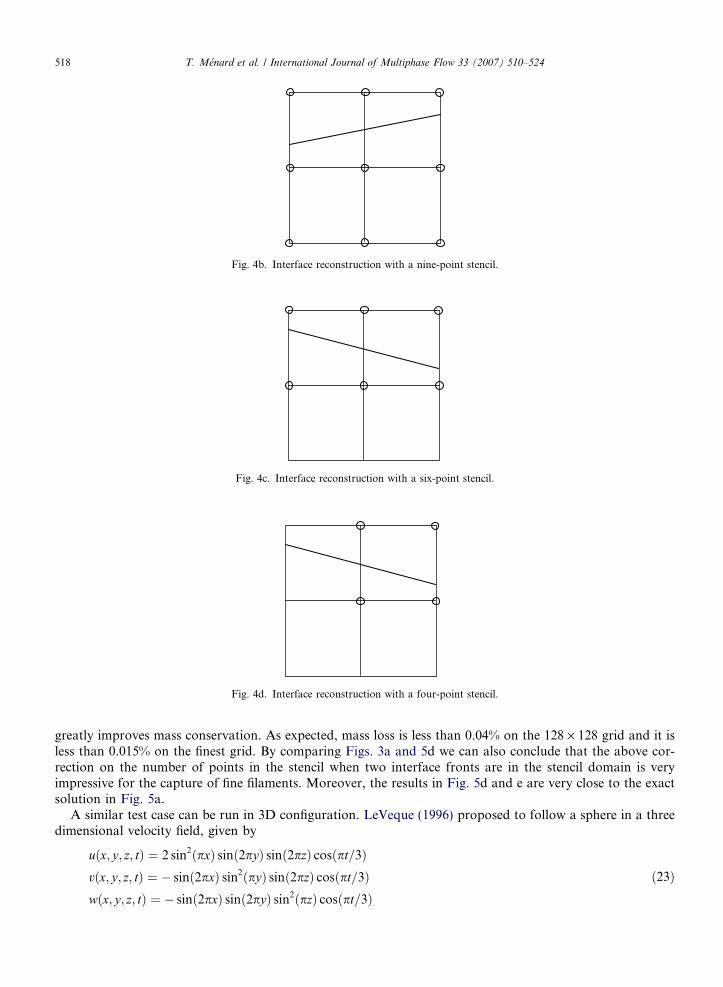
Fig. 4b. Interface reconstruction with a nine-point stencil.

Fig. 4c. Interface reconstruction with a six-point stencil.

Fig. 4d. Interface reconstruction with a four-point stencil.


greatly improves mass conservation. As expected, mass loss is less than 0.04% on the 128 · 128 grid and it isless than 0.015% on the finest grid. By comparing Figs. 3a and 5d we can also conclude that the above cor-rection on the number of points in the stencil when two interface fronts are in the stencil domain is veryimpressive for the capture of fine filaments. Moreover, the results in Fig. 5d and e are very close to the exactsolution in Fig. 5a.

A similar test case can be run in 3D configuration. LeVeque (1996) proposed to follow a sphere in a threedimensional velocity field, given by

uðx; y; z; tÞ ¼ 2 sin2ðpxÞ sinð2pyÞ sinð2pzÞ cosðpt=3Þvðx; y; z; tÞ ¼ � sinð2pxÞ sin2ðpyÞ sinð2pzÞ cosðpt=3Þwðx; y; z; tÞ ¼ � sinð2pxÞ sinð2pyÞ sin2ðpzÞ cosðpt=3Þ

ð23Þ

Fig. 6. Deformation of a sphere: VOF/level set method on a 150 · 150 grid: (a) initial sphere; (b) deformation at t = 1.5 s; (c) return toinitial position t = 3 s; (d) slice of the thin membrane at t = 1.5 s.

Fig. 5. Level set–VOF with stencil correction: (a) 128 · 128 exact solution, Lagrangian method (t = 3 s); (b) 128 · 128 level set;(c): 256 · 256 level set; (d) 128 · 128; (e) 256 · 256.


The domain size is (1,1,1) and the grid size is 150 · 150 · 150. The sphere radius is equal to 0.15 and is cen-tered on (0.35, 0.35, 0.35). Note that a reverse motion is applied on the sphere at t = 1.5 s. As also mentionedby Enright et al. (2002), we observed more than 50% mass loss with the classical level set method. This test casethus appears well adapted to evaluating our 3D coupling between the level set method and the VOF technique.We present in Fig. 6a–c the results of our simulation for the sphere interface at t = 0 s, 1.5 s, and 3.0 s, respec-tively. Slight deviations from the initial sphere geometry are observed at time t = 3 s, but a satisfactory behav-ior of the 3D code is obtained for that quite difficult test case. A slice of the stretched sphere at t = 1.5 s isshown in Fig. 6d and it confirms that no holes are observed in the thin membrane. The computed mass lossis less than 0.03% and the efficiency of our VOF/level set coupling is clearly proved. However, our results arenot as good as Enright’s simulation with the particle level set method. The slight deformations on the spheresurface at time t = 3 s that we observe in our results do not appear in Enright’s results. But the particle level setmethod seems almost impracticable for our purpose, namely the primary break-up of a jet with a large numberof liquid packets.

4. Level set–ghost fluid coupling: dispersion diagram of Rayleigh instability

It is well known that the liquid jet break-up can exhibit different behaviors, depending on various param-eters. The disintegration of a cylindrical plain jet was studied theoretically by Rayleigh (1878). The jet interface


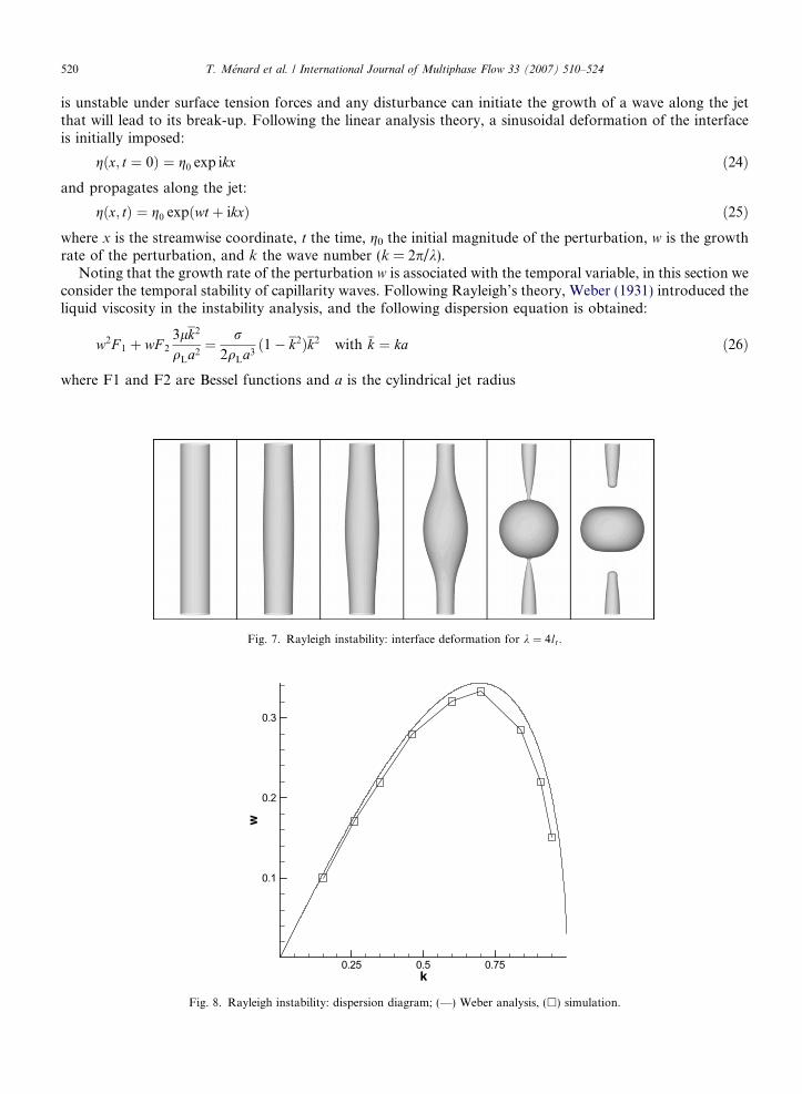
is unstable under surface tension forces and any disturbance can initiate the growth of a wave along the jetthat will lead to its break-up. Following the linear analysis theory, a sinusoidal deformation of the interfaceis initially imposed:

gðx; t ¼ 0Þ ¼ g0 exp ikx ð24Þ
and propagates along the jet:
gðx; tÞ ¼ g0 expðwt þ ikxÞ ð25Þ
where x is the streamwise coordinate, t the time, g0 the initial magnitude of the perturbation, w is the growthrate of the perturbation, and k the wave number (k = 2p/k).
Noting that the growth rate of the perturbation w is associated with the temporal variable, in this section weconsider the temporal stability of capillarity waves. Following Rayleigh’s theory, Weber (1931) introduced theliquid viscosity in the instability analysis, and the following dispersion equation is obtained:

w2F 1 þ wF 2

3lk2

qLa2¼ r

2qLa3ð1� k2Þk2 with �k ¼ ka ð26Þ

where F1 and F2 are Bessel functions and a is the cylindrical jet radius

Fig. 7. Rayleigh instability: interface deformation for k ¼ 4lr.

k

w

0.25 0.5 0.75

0.1

0.2

0.3

Fig. 8. Rayleigh instability: dispersion diagram; (—) Weber analysis, (h) simulation.


Using Eq. (25), a dispersion diagram is obtained for the growth rate of the perturbation as a function of theinitial wave number of the perturbation k.

In the 2D axi-symmetric simulations, the radial length of the domain is lr ¼ 10�3 m; a ¼lr=3; lz ¼ k; k ¼ 2p=k; g0 ¼ 10�4 � Dr, and the initial profile for the level set function is given by

TableJet cha

Diame

100

Phase

LiquidGas

/ðr; zÞ ¼ a� r þ g0 cosð2pz=kÞ ð27Þ
The liquid is water, the gas is air, and the initial velocities are equal to 0. In the radial direction, 61 grid nodesare used, and assuming Dr ¼ Dz, the number of grid nodes in the z-direction is fixed when k (or k) is given.Periodic boundary conditions are assumed in the direction perpendicular to the jet axis, symmetry is assumedon the jet axis, and a free condition is put on the boundary parallel to the axis. In Fig. 7 we present the timeevolution of the interface when k ¼ 4lr.
For each different wave number, the maximum of the growth rate of the perturbation is calculated and thedispersion diagram is presented in Fig. 8. The comparisons between our simulations and the theoretical resultfrom Weber’s analysis (Eq. (25)) are satisfactory. This confirms the interest of using the ghost fluid approach,as we did not succeed in getting the same agreement with the continuous force formulation.

5. A first simulation of 3D jet atomization

In order to illustrate how good the level set/VOF/ghost fluid method is for interface tracking, we present a3D simulation of the primary atomization zone of a turbulent liquid jet. Note that this case is presented heremostly as an illustration of the potentialities of our technique rather than as a reference result.

The main characteristics of the jet are given in Table 1.

1racteristics

ter, D (lm) Velocity (m s�1) Turbulent intensity Turbulent length scale

100 u0=U liq ¼ 0:05 0.1 D

Density ( kg m�3) Viscosity (kg m�1s �1) Surface tension (N m�1)

696 1.2 · 10�3 0.0625 1 · 10�5

Fig. 9. Development of the liquid jet (time step is 2.5 lm).


The size of the domain is (0.0003, 0.0003, 0.0021) in the (x, y, z) directions. To define the mesh size, weassume that no secondary break up occurs for the smallest droplet. This implies that the Weber number isat least smaller than 10 and gives a minimum droplet diameter equal to 2.4 lm. The uniform grid size is thusset to 128 · 128 · 896, and the grid spacing is 2.36 lm. At injection, the Reynolds number U liqD=mliq in theliquid is equal to 5800.

Generation of turbulent inflow boundary conditions is still a challenging task when studying the initialdevelopment of a jet, with an turbulent inlet perturbation. Here, we use the method derived by Klein et al.(2003), which consists in generating correlated random velocities with a prescribed length scale. In our com-putation, that scale is taken as the turbulent integral scale Lt of a cylindrical channel flow ðLt ¼ 0:1DÞ. Withthe above mesh size, it corresponds to four times the grid mesh. The turbulence intensity is equal to 0.05 of themean inlet velocity. The turbulent Reynolds number at injection, based on velocity fluctuations and lengthscale u0Lt=mliq, is equal to 29.

Fig. 10. Liquid jet surface and break-up near the jet nozzle.

Fig. 11. Liquid parcels.

0

0.2

0.4

0.6

0.8

1

1.2

0 2 4 6 8 10 12 14 16 18Axial distance x/D

Liq

uid

pre

sen

ce p

rob

abili

ty

Fig. 12. Liquid presence probability from the level set function on the axis.


The development of the jet is presented on the image sequence (Fig. 9) and the liquid jet surface and break-up near the jet nozzle is presented in Fig. 10. We observe that the first droplets are generated through thebreak-up at the front of the jet (mushroom shape). The main liquid core is thus surrounded by a cloud of smalldroplets.

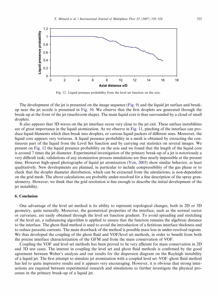
It also appears that 3D waves on the jet interface occur very close to the jet exit. These surface instabilitiesare of great importance in the liquid atomization. As we observe in Fig. 11, pinching of the interface can pro-duce liquid filaments which then break into droplets, or various liquid packets of different sizes. Moreover, theliquid core appears very tortuous. A liquid presence probability in a mesh is obtained by extracting the con-tinuous part of the liquid from the Level Set function and by carrying out statistics on several images. Wepresent on Fig. 12 the liquid presence probability on the axis and we found that the length of the liquid coreis around 7 times the jet diameter. Experimental investigation of the primary break-up of a jet is notoriously avery difficult task; validations of any atomization process simulations are thus nearly impossible at the presenttime. However high-speed photographs of liquid jet atomization (Yon, 2003) show similar behavior, at leastqualitatively. New developments are planned, in particular to include compressibility of the gas phase or tocheck that the droplet diameter distribution, which can be extracted from the simulations, is non-dependenton the grid mesh. The above calculations are probably under-resolved for a fine description of the spray gran-ulometry. However, we think that the grid resolution is fine enough to describe the initial development of thejet instability.

6. Conclusion

One advantage of the level set method is its ability to represent topological changes, both in 2D or 3Dgeometry, quite naturally. Moreover, the geometrical properties of the interface, such as the normal vectoror curvature, are easily obtained through the level set function gradient. To avoid spreading and stretchingof the level set, a redistancing algorithm is applied to ensure that the function remains the algebraic distanceto the interface. The ghost fluid method is used to avoid the introduction of a fictitious interface thickness andto reduce parasitic currents. The main drawback of the method is possible mass loss in under-resolved regions.We thus developed the coupling of the ghost fluid and VOF/level set methods, in order to benefit from boththe precise interface characterization of the GFM and from the mass conservation of VOF.

Coupling the VOF and level set methods has been proved to be very efficient for mass conservation in 2Dand 3D test cases. The interest in coupling the level set and ghost fluid methods is confirmed by the goodagreement between Weber’s analysis and our results for the dispersion diagram on the Rayleigh instabilityof a liquid jet. The first attempt to simulate jet atomization with a coupled level set–VOF–ghost fluid methodhas led to quite impressive results and it appears very encouraging. However, it is obvious that strong inter-actions are required between experimental research and simulations to further investigate the physical pro-cesses in the primary break-up of a liquid jet.


Acknowledgements

Simulations were carried out at the CRIHAN (Centre de Ressources Informatiques de Haute Normandie)and the IDRIS (Institut du Developpement et des Ressources en Informatique Scientifique). We thank alsoMs. D. Moscato for improving the English.

References

Bourlioux, A., 1995, A coupled level-set volume-of-fluid method for tracking material interfaces. In: Proceedings 6th Annual Int. Symp.on Comp. Fluid Dynamics, Lake Tahoe, USA.

Enright, D., Fedkiw, R., Ferziger, J., Mitchell, I., 2002. A hybrid particle level set method for improved interface capturing. J. Comput.Phys. 183, 83–116.

Fedkiw, R., Aslam, T., Merriman, B., Osher, S., 1999. A non-oscillatory Eulerian approach to interfaces in multimaterial flows (the ghostfluid method). J. Comput. Phys. 152, 457–492.

Gueyffier, D., Li, J., Nadim, A., Scardovelli, S., Zaleski, S., 1999. Volume of Fluid interface tracking with smoothed surface stress methodsfor three-dimensional flows. J. Comput. Phys. 152, 423–456.

Kang, M., Fedkiw, R., Liu, X.D., 2000. A boundary condition capturing method for multiphase incompressible flow. J. Sci. Comput. 15,323–360.

Klein, R., Sadiki, S., Janicka, T., 2003. A digital filter based generation of inflow data for spatially developing direct numerical or largeeddy simulations. J. Comput. Phys. 186, 652–665.

LeVeque, R., 1996. High-resolution conservative algorithms for advection in incompressible flow. SIAM J. Numer. Anal. 33, 627–665.Liu, X.D., Fedkiw, R., Kang, M., 2000. Boundary condition capturing method for Poisson equation on irregular domains. J. Sci. Phys.,

151–178.Osher, S., Fedkiw, R., 2003. Level set methods and dynamic implicit surfaces. In: Applied Mathematical Sciences, vol. 153. Springer, New

York.Osher, S., Sethian, J.A., 1988. Fronts propagating with curvature-dependent speed: algorithms based on Hamilton–Jacobi formulations.

J. Comput. Phys. 79, 12–49.Rayleigh, Lord, 1878. On the instability of jets. Proc. London Math. Soc. 10, 4.Rider, W., Kothe, D., 1995 Stretching and tearing interface tracking methods. In: 12th AIAA CFD Conference, 95-1717, AIAA.Sethian, J.A., 1996. Level Set Methods and Fast Marching Methods. Cambridge University Press.Sussman, M., Puckett, E.G., 2000. A coupled level set and volume-of-fluid method for computing 3D and axisymmetric incompressible

two-phase flows. J. Comput. Phys. 162, 301–337.Sussman, M., Smereka, P., Osher, S., 1994. A level set approach for computing solutions to incompressible two-phase flow. J. Comput.

Phys. 114, 146–159.Sussman, M., Fatemi, E., Smereka, P., Osher, S., 1998. An improved level set method for incompressible two-phase. Comput. Fluids 27,

663–680.Tanguy, S., Berlemont, A., 2005. Application of a level set method for simulation of droplet collisions. Int. J. Multiphase Flow 31, 1015–

1035.Unverdi, S.O., Tryggvason, G., 1992. A front-tracking method for viscous, incompressible multi-fluid flows. J. Comput. Phys. 100, 25–37.van der Pijl, S.P., Segal, A., Vuik, C., Wesseling, P., 2005. A mass-conserving level-set method for modelling of multi-phase flows. Int.

J. Numer. Meth. Fluids 47, 339–361.Weber, C., 1931. Disintegration of liquid jets. Z. Angew. Math. Mech. 11, 136.Yon, J., 2003. Jet Diesel haute pression en champ proche et lointain: Etude par imagerie. PhD Universite de Rouen, France.

Coupling level set/VOF/ghost ﬂuid methods: Validation and ...frey/papers/Navier-Stokes/Menard T... · The level set–VOF coupling is validated on 2D and 3D test cases. ... handle

Documents