COUPLING INFORMATION TRANSMISSION WITH AN APPROXIMATE MESSAGE PASSING RECEIVER by David Duncan McNutt Submitted in partial fulfillment of the requirements for the degree of Master of Applied Science at Dalhousie University Halifax, Nova Scotia May 2016 c Copyright by David Duncan McNutt, 2016

Welcome message from author
This document is posted to help you gain knowledge. Please leave a comment to let me know what you think about it! Share it to your friends and learn new things together.
Transcript

COUPLING INFORMATION TRANSMISSION WITH ANAPPROXIMATE MESSAGE PASSING RECEIVER
by
David Duncan McNutt
Submitted in partial fulfillment of the requirementsfor the degree of Master of Applied Science
at
Dalhousie UniversityHalifax, Nova Scotia
May 2016
c© Copyright by David Duncan McNutt, 2016

Dedicated to all of the energetic photons
ii

Table of Contents
List of Figures . . . . . . . . . . . . . . . . . . . . . . . . . . . . . . . . . . . . . v
Abstract . . . . . . . . . . . . . . . . . . . . . . . . . . . . . . . . . . . . . . . . . vii
List of Abbreviations and Symbols Used . . . . . . . . . . . . . . . . . . . . . . . viii
Acknowledgements . . . . . . . . . . . . . . . . . . . . . . . . . . . . . . . . . . xi
Chapter 1 Introduction . . . . . . . . . . . . . . . . . . . . . . . . . . . . . 1
1.1 Summary of Contributions . . . . . . . . . . . . . . . . . . . . . . . . . . 4
Chapter 2 VHF Data Exchange System (VDES) . . . . . . . . . . . . . . . . 5
2.1 The Automatic Identification System . . . . . . . . . . . . . . . . . . . . 5
2.2 Time Division Multiple Access . . . . . . . . . . . . . . . . . . . . . . . . 6
2.3 VDES . . . . . . . . . . . . . . . . . . . . . . . . . . . . . . . . . . . . . 7
Chapter 3 Spatial Graph Coupling . . . . . . . . . . . . . . . . . . . . . . . 9
3.1 Introduction . . . . . . . . . . . . . . . . . . . . . . . . . . . . . . . . . . 9
3.2 LDPC Convolutional Codes Also Known as Spatially Coupled LDPC Codes 10
3.3 Spatial Graph Coupling: From Graphs to Recursion Equations . . . . . . . 13
3.4 Convergence Analysis of Spatially Coupled Systems . . . . . . . . . . . . 19
3.5 Coupling Information Transmission Modulation . . . . . . . . . . . . . . . 233.5.1 Multiple-Access Channel: Single Antenna Receiver . . . . . . . . . 233.5.2 MIMO Block Fading Channel . . . . . . . . . . . . . . . . . . . . 30
Chapter 4 Compressed Sensing Using Message Passing . . . . . . . . . . . 37
4.1 Introduction . . . . . . . . . . . . . . . . . . . . . . . . . . . . . . . . . . 37
4.2 Sparse Estimation Problems . . . . . . . . . . . . . . . . . . . . . . . . . 38
4.3 Inference from Message Passing . . . . . . . . . . . . . . . . . . . . . . . 40
4.4 Message Passing: The Min-sum Algorithm . . . . . . . . . . . . . . . . . 42
iii
Chapter 5 Coupling Information Transmission with
Approximate Message Passing . . . . . . . . . . . . . . . . . . . 44
5.1 System Model . . . . . . . . . . . . . . . . . . . . . . . . . . . . . . . . . 45
5.2 Demodulation and Decoding . . . . . . . . . . . . . . . . . . . . . . . . . 47
5.3 The Proposed AMP-Based Demodulation Algorithm . . . . . . . . . . . . 48
5.4 Numerical Results . . . . . . . . . . . . . . . . . . . . . . . . . . . . . . . 50
5.5 Derivation of AMP Algorithm . . . . . . . . . . . . . . . . . . . . . . . . 51
Chapter 6 Joint Packet Detection and Decoding for Maritime Data Exchange
Systems . . . . . . . . . . . . . . . . . . . . . . . . . . . . . . . . 54
6.1 System Model . . . . . . . . . . . . . . . . . . . . . . . . . . . . . . . . . 556.1.1 Preamble Detection . . . . . . . . . . . . . . . . . . . . . . . . . . 596.1.2 Payload Decoding . . . . . . . . . . . . . . . . . . . . . . . . . . 61
6.2 AMP Algorithm for Joint Decoding and Detection . . . . . . . . . . . . . . 63
6.3 Numerical Results . . . . . . . . . . . . . . . . . . . . . . . . . . . . . . . 63
Chapter 7 Conclusions . . . . . . . . . . . . . . . . . . . . . . . . . . . . . . 66
7.1 Future Work . . . . . . . . . . . . . . . . . . . . . . . . . . . . . . . . . . 66
Bibliography . . . . . . . . . . . . . . . . . . . . . . . . . . . . . . . . . . . . . . 68
iv
List of Figures
Figure 3.1 Unwrapping of Gallager-type (3,6) LDPC matrix H. Taken from [1]. 10
Figure 3.2 Construction of the parity-check matrix Hconv. Taken from [1]. . . . 10
Figure 3.3 Tanner graph of the LDPCC code from Figure 3.2. Taken from [1]. . 11
Figure 3.4 Proto-graph representation of the (3, 6) LDPCC given in Figure 3.2.Taken from [1]. . . . . . . . . . . . . . . . . . . . . . . . . . . . . 12
Figure 3.5 Decoding thresholds for LDPCC codes for varying lengths, L, anddegree profiles under message-passing decoding. Hollow circles de-note block codes, and black circles denote convolutional or coupledcodes. Taken from [1]. . . . . . . . . . . . . . . . . . . . . . . . . 13
Figure 3.6 A diagram representing the Binary Erasure Channel . . . . . . . . . 14
Figure 3.7 Local subtree structure of a large LDPC code . . . . . . . . . . . . 15
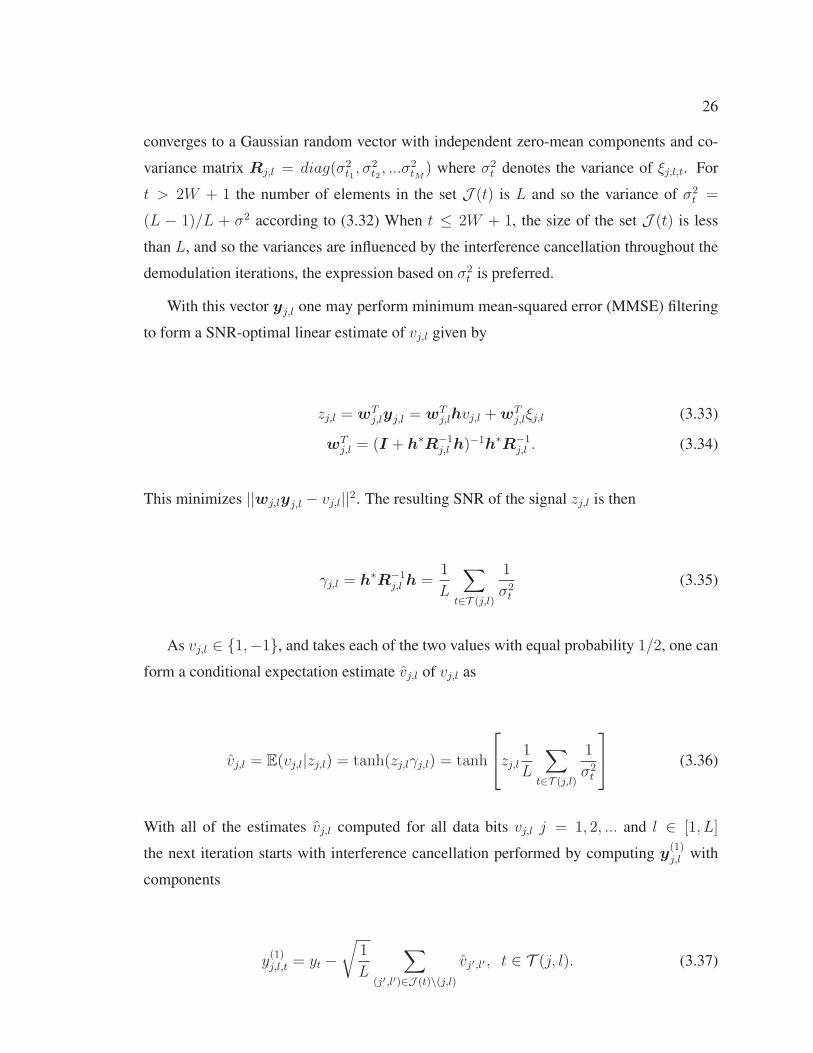
Figure 3.8 Modulation of a binary information sequence for one datastream. . . 24
Figure 3.9 Encoded data bits vj,l are represented by "variable" nodes which areconnected to "channel" nodes representing modulation symbols st.Graphs representing individual data streams are shown in a. Vari-able nodes are depicted as circles while channel nodes are hexagons.The example in b shows the graph obtained by stream coupling withthree datastreams in which the information is modulated into five bitblocks. The transmission time offsets are τ2 = 3 and τ3 = 8. Takenfrom [2]. . . . . . . . . . . . . . . . . . . . . . . . . . . . . . . . 25
Figure 3.10 The relation between variable and channel nodes and the sets ofindices involved. Taken from [2] . . . . . . . . . . . . . . . . . . . 25
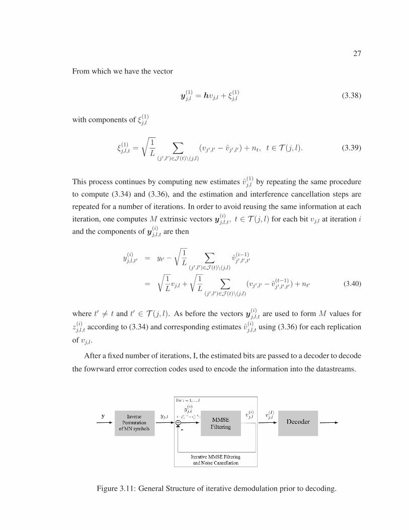
Figure 3.11 General Structure of iterative demodulation prior to decoding. . . . . 27
Figure 4.1 Factor graph associated to the probability distribution (4.9). Circlescorrespond to variables xi, i ∈ [1, n] and squares correspond tomeasurements ya, a ∈ [1,m]. . . . . . . . . . . . . . . . . . . . . . 41
Figure 5.1 Encoding and modulation of the �th data stream. . . . . . . . . . . . 46
Figure 5.2 The MN × MN coupling matrix C consists of identity matricessurrounded by zeros. Each identity matrix IMN corresponds to anincoming data stream and its row offset corresponds to the time off-set (starting time) of that data stream. . . . . . . . . . . . . . . . . . 47
v

Figure 5.3 Diagram of the iterative receiver, with error correction decoding foreach data stream. . . . . . . . . . . . . . . . . . . . . . . . . . . . 48
Figure 5.4 Graph representation of the modulated data. . . . . . . . . . . . . . 49
Figure 5.5 Simulated coupling data transmission with AMP demodulation forM = 250 (solid circles), M = 100 (dashed circles), full message-passing M = 250 (dotted squares), capacity of the GMAC channel(solid curve). . . . . . . . . . . . . . . . . . . . . . . . . . . . . . . 50
Figure 6.1 Encoding and modulation of one data packet. . . . . . . . . . . . . 55
Figure 6.2 A stream of coupled packets with random arrivals of approximately4 packets/packet length. . . . . . . . . . . . . . . . . . . . . . . . . 57
Figure 6.3 The coupling matrix C(Lpack) consists of identity matrices surroundedby zeros. Each identity matrix corresponds to an incoming packetand its row offset corresponds to the packet’s starting time. . . . . . 59
Figure 6.4 Diagram of the iterative receiver that includes joint preamble detec-tion and payload decoding followed by individual error correctiondecoding. . . . . . . . . . . . . . . . . . . . . . . . . . . . . . . . 61
Figure 6.5 AMP based joint decoding and detection algorithm. The above iter-ative process is followed by the individual error correction decodingof the packets. . . . . . . . . . . . . . . . . . . . . . . . . . . . . . 64
Figure 6.6 The throughput achievable by the proposed random access systemin bit/s/Hz as a function of the total system’s SNR. . . . . . . . . . 65
vi

Abstract
Spatial graph coupling has been immensely successful in the field of error correcting
codes. Motivated by this success the coupling approach has been implemented for more
general communication formats, including multiple-access communications. We explore
the application of spatial coupling to modulation of data streams, and employ a recently
proposed approximate message passing compressed sensing technique to develop an al-
gorithm for the demodulation of datastreams transmitted over the multiple-access additive
white Gaussian noise channel and demonstrate that near-optimal sum-rate performance can
be achieved.
vii

List of Abbreviations and Symbols Used
AIS : Automatic Identification System
ALOHA : Not an acronynm; communication protocol
AMP : Approximate Message Passing
ASM : Application Specific Messages
AWGN : Additive White Gaussian Noise
BEC : Binary Erasure Channel
BER : Bit Error Rate
BPDN : Basis Pursuit Denoising
CDMA : Code Division Multiple Access
CRDSA ALOHA : Contention Resolution Diversity Slotted ALOHA
CS-TDMA : Carrier Sense Time Division Multiple Access
dB : Decibels
ECRA ALOHA : Enhanced Contention Resolution ALOHA
FDMA : Frquency Division Multiple Access
IDM : Interleaved-division Multiplexing
IDMA : Interleaved-division multiple access
IMO : International Maritime Organization
IRSA ALOHA : Irregular Resolution Slotted ALOHA
ITU : International Telecommunications Union
viii

LASSO : Least Absolute Shrinkage and Selection Operator
LDPC : Low Density Parity Check
LDPCC : Low Density Parity Check Codes
LP : Linear Programming
MAC : Multiple Acces Channel
MAP : Maximum a Posteriori Probability
MIMO : Multiple Input Multiple Output
MSE : Mean Squared Error
MMSE : Minimum Mean Squared Error
OMP : Orthogonal Matching Pursuit
PS-CDMA : Partitioned Spreading Code Division Multiple Access
S-AIS : Satellite Automatic Identification System
SO-TDMA : Self Organizing Time Division Multiple Access
sup : supremum
TDMA : Time Division Multiple Access
VDES : Very High Frequency Data Exchange System
VHF : Very High Frequency
A : Sensing Matrix
α : Modulation Load or System Load
bl : Preamble Information Bits for lth user
C : Capacity
ix

C : Coupling Matrix
d : A Pseudo-Random Binary Sequence
H t : Channel Matrix at Time t
K or L : Number of Users
M : Repetition Factor
N : Length of Encoded Binary Sequence vl
n,w or ξ : Additive Gaussian Noise Term
P : Total Power of All Users
Pl : Power of lth User
P l : Permutation Matrix for lth User
R : Rate
Ri,t : Covariance Matrix for ith Iteration at Time t
Sl : Signature Sequence Matrix for lth User
σ : Noise Variance
θl : Time Offset for lth Group of Users
vl : Encoded Binary Sequence of lth User
W : Coupling Window
y : Multi-User Received Signal
x

Acknowledgements
First and foremost, I must thank my supervisor Dmitry Trukhachev for his patience and
knowledge. For very similar reasons I would also like to thank my parents Vicki Steeves
and Doug McNutt; as a rule, mathematicians are hard people to deal with.
While completing this degree, I know I could not have done so without my friends.
In particular I’d like to thank Sam Baker, Alisha Dawn Cobham, Paul Dickson, Rachelle
Gammon, Katherine Hurley, Sara Lawlor, Candace MacIntosh and Andy Sears for their
friendship, support, and advice.
xi
Chapter 1
Introduction
The focus of this thesis is on a low-complexity implementation of the coupling informa-
tion transmission multi-user communication technique based on the spatial graph coupling
principle [3]. Each user transmits one or more independently encoded data streams over
the multiple access channel. Each data stream is encoded and modulated such that the
relations between the data bits and modulation symbols within each transmitted stream
are represented by a bipartite graph. The data streams are transmitted with time offsets
enabling coupling of the transmitted graphs into a single continuous graph chain at the re-
ceiver. Modulation of each data stream is accomplished with repetition, permutation, and
spreading of data.
The principle of spatial graph coupling [4, 5, 6] which originated in the area of low-
density error-correction codes, has recently attracted significant research attention. Con-
struction of coupled graph models on which sub-optimal iterative message-passing de-
coding can asymptotically achieve the optimal maximum a posteriori probability (MAP)
decoding limit has now been applied in a number of fields including multiple-access com-
munications. Regular (un-coupled) random code-division multiple access (CDMA) [7] as
well as its sparse counterparts [8, 9, 10] can only achieve limited multi-user loads of equal
power users. The application of spatial graph coupling removes this limitation [2, 11, 12],
and in addition, can make the system capacity-achieving asymptotically [2, 11].
The receiver performs iterative message-passing interference cancellation and data es-
timation on the received graph chain, followed by individual error-correction decoding,
performed for each data stream individually, providing near-capacity operation [2, 11].
Slightly different modulation graphs resulting from partition-spreading CDMA [9], gener-
alized modulation [13], interleaved-division multiple access (IDMA) [14], sparse CDMA
[8], and, interleaved-division multiplexing (IDM) [15] result in similar coupled equations
characterizing the iterative interference cancellation behaviour at the receiver.
In practice, however, achieving high multi-user loads and spectral efficiency requires
1
2
large amount of data streams and large repetition factors. This presents a challenge for
the existing message-passing algorithms in terms of both memory and computational com-
plexity. To make the modulation format based on spatial graph coupling practical we must
consider an appropriate receiver. We introduce a demodulation technique based on ap-
proximate message passing (AMP) proposed by Donoho et al. [16] for compressed sensing
problems.
A version of the AMP is specially derived for our multi-user situation and allows for
efficient implementation, a large savings in complexity, and simplified operation in the
“near-capacity” regime. The demodulation complexity per bit is constant per iteration and
does not scale with the processing gain, contrary to existing algorithms [2, 11, 12]. The
algorithm is first derived for the theoretic case in which users transmit their data streams
at specific times, and then extended to the case where the packets arrive at random times
considering a particular application of the technique.
As an application we adapt our modulation/demodulation approach to address random
channel access in maritime data exchange systems. These systems have received signifi-
cant research attention in recent years due to the rapidly growing number of vessels and
information services required for their operation including positioning, tracking, and navi-
gation. While the automatic identification system (AIS) has proven to be a very successful
means of tracking ships, the capacity of AIS will soon be exceeded; in some ocean areas,
such as the Gulf of Mexico, the current AIS load is already above 50% of its capacity [17].
At the same time new applications such as e-navigation require additional capabilities to
exchange data.
The new standard of VHF data exchange (VDES) which is currently under development
by the International Telecommunications Union (ITU) will include satellite ship track-
ing, ship-to-shore, and ship-to-ship communication and extend the services provided by
AIS [18]. Random access communications will be an important mechanism of accessing
the communication channel resources in VDES. The current time-division based random
access (TDMA) mechanism in AIS may not be suitable for the upcoming traffic demands
for VDES. This suggests that a new random access mechanism must replace TDMA.
We focus on an uplink communication scenario in which multiple number of vessels
transmit their messages to a satellite charing the same communication channel. We pro-
pose a way to apply coupling data transmission in a random access fashion, using the AMP
3
algorithm at the receiver. To do so we adapted our modulation scheme to include the trans-
mission of a preamble prior to sending each datastream’s payload. Similarly for demodu-
lation at the receiver, preamble detection was inserted into the iterative loop for the AMP
algorithm, its convergence is studied and we demonstrate that the achievable multi-user
loads are superior to that of competing random-access systems.
The thesis is divided into five subsequent chapters and a conclusion. In Chapter 2 VHF
maritime data exchange systems are introduced. Current TDMA media access schemes and
the limitation of these for the future application in maritime data exchange are discussed.
In Chapter 3 the theory behind the spatial graph coupling method is introduced using
low-density parity-check convolutional codes - the original coupled system. After that two
examples describing applications of spatial graph coupling to multi-user communications
are given. The first example discusses the coupling information transmission [2] for the
multiple access AWGN channel with single antenna at the receiver, while the second ex-
ample is an original contribution for the multiple input and multiple output (MIMO) case
where the receiver has two antennas. The chapter discusses the original message-passing
interference cancellation receiver for the coupling information transmission.
Chapter 4 discusses sparse estimation problems and the variety of approaches used for
reconstruction of information. The basic theory behind message-passing algorithms on
graphs is introduced and a particular example, the min-sum algorithm is discussed. The
chapter concludes with a summary of the cost function and messages used for the message-
passing algorithm used in the receiver for the coupling information transmission.
Modulation for communication over the AWGN channel where arrival of each datas-
tream is known, using spatial graph coupling is elaborated on in Chapter 5. Specifically, the
approximate message passing algorithm is presented and used to demodulate the received
signals. Numerical results are provided to illustrate the efficiency of the AMP based de-
modulation. The chapter concludes with a mathematical derivation of the AMP algorithm
from the message-passing rules introduced in Chapter 3 and using compressed sensing
approach from Chapter 4.
In Chapter 6, we consider the modulation for communication over the AWGN channel
where users access the channel randomly. This chapter is dedicated to the application to the
maritime data exchange systems and in particular to the uplink to satellite scenario. The
main feature of the development is the iterative reception in which detection of packets

4
and the multi-user demodulation is happening in parallel. Simulation results highlighting
various system loads are presented.
Finally, Chapter 7 presents the conclusion and an outlook on the future work.
1.1 Summary of Contributions
The work presented in this thesis contributes to improving the efficiency of communi-
cation over the AWGN multiple access channel by exploiting spatial graph coupling and
techniques from compressed sensing. As a result of this effort, two papers have been pre-
pared for publication:
� D. Truhachev, and D. McNutt (2015)
Coupling Information Transmission with Approximate Message Passing, IEEE Com-
munications Letters, under revision.
� D. Truhachev, and D. McNutt (2015).
Joint Packet Detection and Decoding for Maritime Data Exchange Systems. MT-
S/IEEE Oceans 2015.
The first paper is based on the work presented in Chapter 5 which focuses on the trans-
mission of data from multiple users over the multiuser AWGN channel. The focus is on
a theoretic setup in which arrival for each signal is assumed to be known, and all users
transmit with equal power. The derivation of the AMP algorithm, and numerical simu-
lations illustrating the achievable sum-rate of the algorithm in conjunction with coupling
transmission are presented.
The second paper was published in the proceedings of the international conference
MTS/IEEE Oceans 2015. This paper is based on the work presented in Chapter 6 where we
consider the transmission of data from multiple users over the MAC AWGN channel where
the packets arrival are now random. Each transmitting user forms a packet and includes a
preamble to the message payload in order to ensure detection, demodulation and decoding
at the receiver. In this paper we outline how the AMP algorithm derived in Chapter 5 can
be adapted to allow for the detection of packets using pseudo-random binary sequences
that are known to the receiver, and present the performance of this system in terms of total
throughput of the system versus signal-to-noise ratio. The impact of the carrier frequency
shift due to the satellite’s motion is also taken into account.

Chapter 2
VHF Data Exchange System (VDES)
2.1 The Automatic Identification System
Due to the rapidly growing number of vessels and the increasing number of information
services required for ship operation there has been a significant research effort directed at
improving maritime data exchange systems. One important component of these exchange
system has been the automatic identification system (AIS) used by ships and by vessel
traffic services to identify and locate vessels by exchanging data with other nearby ships,
shore base stations, and satellites.
The automatic identification system (AIS) supplements marine radar as a secondary
method of collision avoidance for water transport. The International Maritime Organi-
zation (IMO) requires AIS to be fitted aboard any ship with gross tonnage equal to 300
or more, and all passenger ships. The information provided by this system consists of a
unique identification, position, course, and speed for each ship. This allows for maritime
authorities and each vessel’s watchstanding officers to track and monitor vessel movements.
In order to record and transmit this information AIS integrates a standardized VHF
transceiver with a positioning system receiver, electronic navigation sensors and a gyro-
compass or rate of turn indicator. Any vessel fitted with AIS transceivers can be tracked by
AIS base stations, or when out of range of terrestrial networks through satellites that have
been equipped with special AIS receivers which can manage the large number of vessel
signatures. Outside of collision avoidance, many applications have been developed for AIS
including fishing fleet monitoring and control, vessel traffic services, marine security, aids
to navigation, search and rescue, accident investigation, and fleet and cargo tracking.
Terrestrial AIS uses two globally allocated Marine Band Channels 87 and 88 with trans-
mitting frequencies 161.975 MHz and 162.025 MHz respectively, the system transmits
using Gassian minimum shift-keying (GMSK). AIS uses the frequency channels by em-
ploying frequency division duplexing, where the upper leg of these channels are used for
shore-to-ship and ship-to-ship digital messaging, while the lower leg of the channels is used
5

6
for ship-to-shore messaging.
In contrast, ship-to-satellite messages (long range AIS) uses the Maritime Band chan-
nels 75 and 76 with frequencies 156.775 MHz and 156.825 MHz. Currently the ships only
transmit to satellites, with no messages received from the satellites in order to provide nav-
igational information for all ships. For this reason, there is no need for duplex channels
when long range AIS is used [19]
While ship-to-ship and ship-to-shore have a range of ten to twenty miles, Satellite-AIS
(S-AIS) has a much larger coverage. Shipboard AIS transceivers can reach much further
vertically; up to the 400 km orbit of the International Space Station (ISS). Since satellite
receive footprint is hundreds of miles in radius, such receiver needs to be able to handle a
huge number of vessel signatures.
By its very nature, AIS must allow vessels to access the channel without interfering with
each other, the AIS transceivers use Time Division Multiple Access (TDMA) to transmits
and receive messages. The AIS standard comprises several sub-standards (or types) for
individual products, but there are two major product types for vessel-mounted transceiver:
� Type A : Targeted at large commercial vessels, these transceivers use Self-Organized
TDMA (SO-TDMA) as a method of random channel access.
� Type B : Targeted at smaller commercial and leisure vessels, there are two subtypes
depending on whether SO-TDMA or Carrier Sense TDMA (CS-TDMA) is used as a
method of random channel access by the transceiver.
2.2 Time Division Multiple Access
Time division Multiple access allows multiple users to share the same frequency chan-
nel by dividing each minute frame into 2250 slots, during which users transmits one after
another. How this slot structure is accessed is determined by the chosen scheme.
� Self Organized-TDMA :
This is the multiple access approach associated with the Class A transceivers. Each
user maintains an updated slot map in its memory allowing for prior knowledge of
available slots. This is achieved by sharing a common time of reference derived from
7
GPS time. Before a message is sent the user will pre-announce their transmission
in a known free slot indicating their intention to use a particular slot for the next
transmission. This allows other users to update the slot map, and avoid those slots
that are known to be in use [19].
As users move in and out of communication regions, they will encounter new users
with different slot allocations, causing the slot map to be recomputed. From these
rules a dynamic and self organizing system over time and space can be determined.
� Carrier Sense-TDMA :
This is the multiple access approach associated with the Class B transceivers. The
access scheme is fully interoperable with SO-TDMA transmission, and also ensures
priority is given to SO-TDMA transmissions. To do this, a user using CS-TDMA
determines the slot timing by observing the timing of a user using SO-TDMA. Then,
by continuously monitoring the channel background noise level, the user can use this
as a reference for a received signal strength measurement at the start of each TDMA
slot.
When a transmission is required, a TDMA slot is picked at random and if the signal
strength at the start of the slot is above the background level, the slot is assumed to
be in use and the transmission is deferred, otherwise the slot is assumed to be empty
and the slot used. There are limitations to this approach, this will only work on a slot
by slot basis, unlike SO-TDMA which can use multiple concurrent slots.
In terrestrial AIS, SO-TDMA allows for autonomous management of capacity in busy
areas, by implementing "slot-reuse rules" when all TDMA slots are occupied. The slots
occupied by the most distant users are re-used for local transmission. This reduces the size
of an AIS region and ensures position reports from closer users are not affected. This is
important as these users are most relevant to navigation. This approach no longer works in
satellite AIS when a satellite receives many messages from many vessels.
2.3 VDES
As AIS usage increased globally in terms of number of vessels and variety of applica-
tions related to AIS grow, the ITU Radiocommunication Assembly have recognized that
8
a new VHF data exchange system must be introduced to accommodate the growing num-
ber of users, and the diversification of data communication applications. This system will
allow for harmonized collection, integration, exchange, presentation, and analysis of ma-
rine information onboard and ashore to enhance berth to berth navigation, and associated
services for safety and security at sea.
While the proposed VHF data exchange system will incorporate other maritime safety
related applications outside of the scope of AIS, it must improve AIS functionality in order
to allow for increased usage of the channel. Running continuously, this implementation
must ensure that the functions of digital selective calling, AIS and voice distress, safety,
and calling communication are not impaired.
VDES will require multiple frequency channels in the VHF band for AIS, application
specific messages (ASM), voice and other data communication needs such as e-navigation
[17].
Current time-division based random access (TDMA) mechanism in AIS has a number
of limitations such as the necessity to maintain slot maps and limitations imposed by the
number of available slots. Specifically in satellite uplink communication with a large pop-
ulation of users accessing the channel that coordinating channel access will be difficult due
to the finite number of slots per minute per frame, and the difficulty to organize slot maps
due to large feedback delays. Hence, alternative, more flexible media access approaches
would be desirable for VDES. In particular random media access and multi-packet recep-
tion would provide a very useful functionality in this scenario. Chapter 6 is this thesis
describes a potential application of the coupling information transmission technique with
an AMP receiver for VDES communication scenarios.
Chapter 3
Spatial Graph Coupling
3.1 Introduction
Error-correction codes on sparse graphs such as low-density parity-check codes (LDPC)s
that have been a popular theoretic area of research codes are frequently used in practical
communications by now. LDPCs are included in a numerous sttandards such as wireless
local-area networks WiFi [20], WiMax, digital video broadcasting DVB-S2, 10GBase-T
Ethernet and others. Due to the ubiquity of iterative belief-progagation-based decoding
of sparse graphical codes, and their incorporation into many communications standards,
it would be beneficial to construct new codes based on these algorithms that are formally
capacity achieving.
While it is known that polar codes achieve channel capacity [21], these are not easily
implemented for applications. With this in mind, it has been proven that a collection of
sparse codes that are spatially coupled will have an improved decoding threshold which
approaches the maximum-aposteriori decoding (MAP) of the uncoupled sparse code [6,
22]. This is known as threshold saturation. Originally the concept of spatial graph coupling
arose from the construction of convolutional low-density parity-check codes (LDPCCs)
by Felström and Zigangirov [4], spatial graph coupling has been readily adapted to other
applications like source coding and multiple access communications.
Whatever the application of spatial graph coupling may be, the method involved is
essentially equivalent to the case of coupling graph-based error control codes. For this
reason we will introduce the concepts of spatial graph coupling in the guise of an exposition
of LDPCCs on the Binary Erasure Channel (BEC), before generalizing into the framework
of coupled vector recursions. As a way to sidestep the issues involved in proving threshold
saturation for the spatially coupled codes, we conclude with an introduction to Lyapunov
stability theory; which will allow one to prove that a coupled system may attain the capacity
of the transmission channel.
9
10
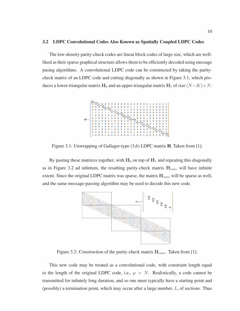
3.2 LDPC Convolutional Codes Also Known as Spatially Coupled LDPC Codes
The low-density parity-check codes are linear block codes of large size, which are well-
liked as their sparse graphical structure allows them to be efficiently decoded using message
pasing algorithms. A convolutional LDPC code can be constructed by taking the parity-
check matrix of an LDPC code and cutting diagonally as shown in Figure 3.1, which pro-
duces a lower-triangular matrix H0 and an upper-triangular matrix H1 of size (N−K)×N :
Figure 3.1: Unwrapping of Gallager-type (3,6) LDPC matrix H. Taken from [1].
By pasting these matrices together, with H0 on top of H1 and repeating this diagonally
as in Figure 3.2 ad infintum, the resulting parity-check matrix Hconv will have infinite
extent. Since the original LDPC matrix was sparse, the matrix Hconv will be sparse as well,
and the same message-passing algorithm may be used to decode this new code.
Figure 3.2: Construction of the parity-check matrix Hconv. Taken from [1].
This new code may be treated as a convolutional code, with constraint length equal
to the length of the original LDPC code, i.e., μ = N . Realistically, a code cannot be
transmitted for infintely long duration, and so one must typically have a starting point and
(possibly) a termination point, which may occur after a large number, L, of sections. Thus

11
Hconv will be a band-diagonal matrix of size L(N − k) × LN . The effect of terminating
at either or both ends of the code is ultimately beneficial, as the ratio of information bits
to coded bits is locally smaller around the termination points, and so a locally improved
bit error rate is expected. It turns out that this improvement is carried out to the entire
codeword via iterative decoding.
Just as in the original case of an LDPC block code, we may construct a Tanner graph
of a convolutional LDPC code, which illustrates the band-diagonal structure of the parity-
check matrix. Drawing the graph in sections as in Figure 3.3, it is easily seen that the first
bits are checked by lower weighed check nodes than in the remaining sections. This may
be treated as having the earlier bits before the starting point known in advance, and hence
set to zero.
Figure 3.3: Tanner graph of the LDPCC code from Figure 3.2. Taken from [1].
Unlike the example given in Figure 3.3, the originating LDPC code must be much
larger, and in practice N ≈ 103 and larger are typical for practical applications. The
Tanner graph for such a code would be too confusing to be used as a conceptual tool,
instead we consider a proto-graph representation of the code, given in Figure 3.4, where
each edge of the proto-graph represents N2
edges, connecting N2
variable nodes and check
nodes respectively. Each of the N2
pairs of nodes are connected by a permuted arrangement
of the edges, with each of the proto-graph edges representing a different permutation.
Each section in Figure 3.4 represents a N -sized section of the convolutional LDPC
code. From this perspective one can see that the endpoints of the structure have better
protections; the parity nodes at either end have degree two, followed by nodes with degree
four, and the remaining interior nodes have degree six, and all variable nodes have degree
three While there is some rate loss associated with termination of the code, one may see

12
Figure 3.4: Proto-graph representation of the (3, 6) LDPCC given in Figure 3.2. Takenfrom [1].
that as L → ∞ the design rate of the LDPCC code is
R = limL→∞
1− (L+ 1)(N −K)
LN=
K
N, (3.1)
just like for the block LDPC, R = 1L
for the (3,6) code case.
The decoding threshold for convolutional LDPCs generated from regular (J, 2J) LDPC
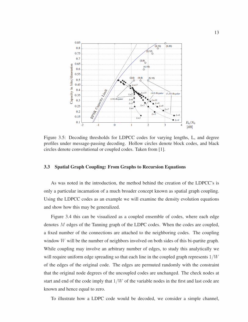
codes was studied in [5, 23], and is summarized in Figure 3.5 for several lengths, L, of the
structure. Notice that as L → ∞, those regular codes with large J achieve a threshold that
reaches the capacity limit of the binary-input AWGN channel at Eb/N0 = 0.19dB with
rate R = 0.5, this is defined as
Definition 3.2.1. The iterative decoding threshold of a code family is the largest channel
parameter ε∗ (for BEC) or smallest SNR∗ (for AWGN) such that for any ε < ε∗ (SNR >
SNR∗) the decoding error probability of iterative message passing decoding goes to 0
as a function of the code length N with constraint length μ and the number of decoding
iterations I . Typically exponential error probability decay is a function of N(μ) is required
as well.
Alternatively for small L the rate loss experienced by the LDPCC code given by the
formula (3.1) will be smaller than the rate of the block version of the same code, and hence
codes with lengths significantly larger than ten are required to achieve the same threshold.
Admittedly, for most applications the effort involved for the gain in threshold may not be
necessary, as the code lengths in the block code case required to gain a fraction of a dB in
terms of performance will be on the order of 100,000 compared to 1,000-10,000 of the base
code. The interest in convolutional LDPCs lie in the connection to spatial graph coupling
which allows for the construction of message-passing code ensembles that are proven to
achieve the Shannon’s capacity limit.
13
Figure 3.5: Decoding thresholds for LDPCC codes for varying lengths, L, and degreeprofiles under message-passing decoding. Hollow circles denote block codes, and blackcircles denote convolutional or coupled codes. Taken from [1].
3.3 Spatial Graph Coupling: From Graphs to Recursion Equations
As was noted in the introduction, the method behind the creation of the LDPCC’s is
only a particular incarnation of a much broader concept known as spatial graph coupling.
Using the LDPCC codes as an example we will examine the density evolution equations
and show how this may be generalized.
Figure 3.4 this can be visualized as a coupled ensemble of codes, where each edge
denotes M edges of the Tanning graph of the LDPC codes. When the codes are coupled,
a fixed number of the connections are attached to the neighboring codes. The coupling
window W will be the number of neighbors involved on both sides of this bi-partite graph.
While coupling may involve an arbitrary number of edges, to study this analytically we
will require uniform edge spreading so that each line in the coupled graph represents 1/W
of the edges of the original code. The edges are permuted randomly with the constraint
that the original node degrees of the uncoupled codes are unchanged. The check nodes at
start and end of the code imply that 1/W of the variable nodes in the first and last code are
known and hence equal to zero.
To illustrate how a LDPC code would be decoded, we consider a simple channel,

14
namely the Binary Erasure Channel BEC given in Figure 3.6, where each bit transmit-
ted has a probability ε ∈ (0, 1) of being erased.
Figure 3.6: A diagram representing the Binary Erasure Channel
Consider a (dv, dc) LDPC block code, i.e., dv edges come out of each variable node and
dc edges from a check node. We denote A = {−1, 0,+1} as the channel output, ri ∈ A the
received symbol at variable node i, and di ∈ A the decision at variable node i. A message
from variable node i to check node j is represented by ui→j ∈ A and a message from check
node j to variable node i is βj→i ∈ A. Finally we write Vj\i as the set of variable nodes
which connect to check node j, except for variable node i, and Ci\j to be the set of check
nodes which connect to variable node i, excluding check node j. To decode an LDPC code
on the BEC, we have the following steps:
1. Initialize di = ri for each variable node. If ri = 0 then the received symbol i has
been erased and variable i is said to be unknown.
2. Variable nodes send μi→j = di to each check node j ∈ Ci
3. Check nodes connected to variable node i send βj→i = Πl∈Vj\iul→j to i. I.e., if all
incoming messages are different from zero, the check node sends back to i the value
that makes the check consistent, otherwise it sends back a zero for “unknown”.
4. If the variable i is unknown and at least one βj→i �= 0 set di = βj→i and declare the
variable i to be known. For the simple BEC, once a variable is known its status can
not be changed.
5. When all variables are known, stop. Otherwise go back to Step 2.
To study the behaviour of this decoding scheme, density evolution analysis allows a
recursive relation to be derived describing the statistical behaviour of a regular block LDPC
code over the binary erasure channel (BEC) ([1], section 6.2) we consider the tree structure

15
given in Figure 3.7. Let ε(l)v denote the probability of erasures at the variable nodes at
iteration l, and ε(l)u be the probability of erasures at the check nodes at iteration l, then for a
regular code, in which the node degrees are all equal, the following recursive relation can
be established
ε(l−1)u = 1− [1− ε(l−1)
v ]dc−1, ε(l)v = ε[ε(l−1)u ]dv−1 (3.2)
starting with ε(0)u = ε with ε is the initial probability of erasure.
Figure 3.7: Local subtree structure of a large LDPC code
Combining these two equations produces a one-dimensional iterated map for the prob-
ability that any variable node remains uncorrected ,
x(l) = f(x(l−1), ε) = ε(1− [1− x(l−1)]dc−1)dv−1, (3.3)
where x(l) is the probability of bit erasure at iteration l in a (dv, dc) regular LDPC block
code of infinitely large size N → ∞. We need this to ensure that there is a tree-like
neighborhood of decoding for each symbol. We define a check node function in (3.3) as
g(x) = 1− (1− x)dc−1, (3.4)
16
and the statistical variable node function as
f(y, ε) = εydv−1, (3.5)
the dynamic behaviour of a regular LDPC code may be characterized by the fixed points of
the equation
x = f(g(x), ε). (3.6)
The above equation has one fixed point at x = 0, but can have two or three depending
on ε, and the supremum of ε such that only one fixed point exists, we say ε∗ is called the
belief propagation threshold (BP threshold). For this system, convergence to the limit point
x(∞) = 0 requires
x− εf(g(x), ε) > 0, x ∈ [0, ε]. (3.7)
Alternatively, we may formulate the threshold value of the parameter ε as
εs = sup{ε s.t. x(∞) = 0}. (3.8)
Through numerical experimentation, it may be shown that the largest erasure probability
that can be corrected by the code is ε = 0.4294. for the (3,6) code [1].
In the coupled case, we must consider the convergence behaviour of each system in-
volved in the coupled ensemble, thus we must consider a vector convergence equation of
the form
x = F (x, ε), (3.9)
where x = [x1, ..., xL] is a vector of the statistical variable for each of the L + 1 coupled
dynamical systems illustrated in figure 3.4, and F is a monotonic decreasing function.
Returning to the coupled system of L copies of L graphs, with a uniform window of size

17
W , the variables are updated as
x(l+1)i =
1
W
W−1∑k=0
f
(1
W
W−1∑j=0
g(x(l)i+j−k, ε
)). (3.10)
The boundary conditions may be imposed by requiring that xl = 0 for l /∈ [0, L], which
corresponds to variables that are already known, which may be pilot signals, frame markers,
preambles or any other fixed signals we wish to couple to our code ensemble.
Writing this in vector form, we denote the vector functions f(x, ε) and g(x) which
operate on each components of the vector x as a scalar with f(·) and g(·) respectively.
Then equation (3.10) may be expressed as
x(l+1) = ATf(Ag(x(l), ε)
))= F (x(l), ε), (3.11)
where A is a band-diagonal matrix with non-zero entries 1/W for all j ≥ i and j−1 ≤ W ,
and zeros otherwise.
The parameter ε in this instance represents the channel erasure probability. More gen-
erally it could be a signal to noise ratio, or another parameter characterizing the channel.
Typically one is interested in the threshold of the coupled system which is the largest ε such
that an arbitrary initial vector x(0) converges to the zero vector.
Denoting the set of all possible values of the erasure probabilities for each system x as
X 0, these will be strictly non-negative and hence the form of (3.11) implies
F (x, ε) ≤ x and F (x, ε) ∈ X 0. (3.12)
Thus for any l > 0 and x(l) ∈ X 0 we have that x(l+1) ≤ x(l) and x(l+1) ∈ X 0, and so we
will have a monotonically non-increasing sequence of points if we continue to iterate the
equation. If we can find some initial point x(0) such that the resulting sequence of points is
strictly monotonically decreasing, i.e., x(0) > x(1) > x(2) > ... then this must converge to
a limiting point x(∞) ≥ 0. Ideally this point should be a stable fixed point, it is possible for
particular values of ε that there are unstable fixed points where the system passes through
this fixed point and moves towards another fixed point.
The boundary conditions play an important role in the convergence of the coupled sys-
tem, as these allow the dynamical variables xl closer to the exterior of the ensemble to
18
converge faster than the interior variables. This allows for the boundary conditions to prop-
agate to the interior of the system over several iterations, which would not be possible
without the boundary conditions.
To study the convergence of the system (3.11), an approach was introduced by [24] and
expanded upon in [25, 26] which was based upon the function U(x, ε) : x → R1 called the
potential function
U(x, ε) =
∫ x
0
g′(z)[z − f(g(z), ε)]dz. (3.13)
whose origin arose from the continuous-time approximation for the system (3.11) given by
dx(t)
dt= F (x(t), ε)− x(t), t > 0, t → ∞. (3.14)
With this function we have a general result for any recursion equation of the above form:
Theorem 3.3.1. For large window sizes w → ∞, an iterative system of sparse graphs
couples as in (3.11) converges to x(l) → 0, if U(x) > 0. This implies that the coupled
system threshold may be given by the following criteria:
ε∗c = sup{ε : U(x, ε) > 0, ∀x ≤ ε}. (3.15)
Using this theorem, it may be shown that the coupled (3,6) LDPC code ensemble for the
BEC channel will converge for erasure rates up to ε = 0.48815 which is much closer to the
capacity CBEC = 0.5 than the uncoupled case.
In general, for large w ≥ 0, ε∗c ≥ ε∗; coupling always improves performance. Exploit-
ing theorem 3.3.1, it can be shown that certain convolutional LDPC codes based off the
(dv, dc) LDPC codes achieve capacity over the binary erasure channel [1]:
Theorem 3.3.2. For large window sizes, w → ∞, an iterative system of sparse coupled
regular (dv, dc) LDPC codes achieve the capacity of the BEC,
ε∗c → α, for α =dvdc, and dv → ∞.
Equivalently, the rate of the code R = 1 − dv/dc approaches the channel capacity, R →1− ε = CBEC for ε → ε∗c .

19
The proof follows by computing the potential function for the regular (dv, dc) LDPC codes:
U(x, ε) =1
dc− (1− x)dc
dc− x(1− x)dc−1 − ε
dv
(1− (1− x)dc−1
)dv. (3.16)
and determining the largest ε∗ for which U(x, ε∗) ≥ 0 for all x ∈ [0, 1].
The phenomenon of threshold saturation is in fact very general [6], and has been shown
to be applicable to other communication scenarios such as the isotropic multiple access
channel used with uniformly random signal sets [2]. For this reason it is important to show
rigorously, whatever the application, that the coupled system converges to the zero vector.
In the case of the LDPCC codes one is able to work with the potential function which
exists as the original recursion equation is scalar-valued. In the case of vector recursions,
the existence of a potential function is no longer assured. In the next section we will explore
a related tool that will help determine convergence.
3.4 Convergence Analysis of Spatially Coupled Systems
From the previous section we have seen that the performance of spatially coupled en-
sembles of LDPC codes relied on the convergence, to the point x(∞) = 0, of an iterative
vector recursion equation:
x(l+1) = F (x(l), ε), F (x, ε) ≤ x and F (x, ε) ∈ X 0. (3.17)
We will focus on the case where x is non-increasing, however it should be noted that there
may be other stable points such that x(∞) �= 0 which might cause a small initial value
of x(0) to move towards a non-zero fixed point; given the current application these points
should be avoided as they are not helpful for applications.
If we pick an initial point x(0) such that the resulting sequence of points is strictly
monotonically decreasing, i.e., x(0) > x(1) > x(2) > ..., then the sequence will converge
to some limiting point x(∞)(x(0), ε) ≥ 0. We wish to determine when a given vector
recursion will converge to the point x(∞)(x(0), ε) = 0 for a particular ε. This question may
be approached using the Lyapunov method. This will simplify the behaviour of individal
trajectories in a dynamical system, like the one given above, to the study of the system’s
20
properties in subspaces of X 0 through the study of Lyapunov functions [27].
As before, X 0 denotes the smallest set containing x(l) for all l ≥ 0 and we introduce
an open subset X 1 ⊂ X 0 such that 0 /∈ X 1. For the domain of ε, E , we have two subsets
E0 = E \{0} and E2 ⊂ E0. The purpose of E2 will be explained momentarily, but this subset
willl be related to the issue of global asymptotic stability.
Definition 3.4.1. The solution x(l) = 0 to (3.11) is globally asymptotically stable if
liml→∞ x(l) = 0 for all x(0) ∈ X 0.
Lyapunov introduced a special type of function in X 0 defined by the following criteria:
Definition 3.4.2. A continuous function V (x) : X → R1 is called a Lyapunov function for
the system (3.11) with x ∈ X 0, ε ∈ E2 if it satisfies the following conditions:
V (0) = 0, (3.18)
V (x) > 0 for x ∈ X 1, (3.19)
V (f(g(x), ε))− V (x) < 0 for x ∈ X 1, ε ∈ E2. (3.20)
We may provide sufficient conditions for global asymptotic stability of the system (3.11)
Theorem 3.4.3. Given that V (x) is a Lyapunov function for the system (3.11) for ε ∈ E2,the solution x(l) = 0 is globablly asymptotically stable.
Thus for any ε ∈ E2, any initial choice of x(0) will converge to the origin 0.
While this was formulated for a continuous system, this may be related to the iterative
equation (3.11) by writing this as
x(l) − x(l+1) = q(x(l)) = x(l) − F (x(l).ε) (3.21)
We may build a Lyapunov function for this system by considering its continuous-time ana-
log,
dx(t)
dt= −q(x(t)), t > 0, t → ∞. (3.22)
We use the variable gradient method to construct a Lyapunov function for this new system
that satisfies (3.18) - (3.20). Let V : X → R1 be a continuously differentiable function

21
with
h(x) =
(∂V
∂x
)T
=
[∂V
∂x1
, ...,∂V
∂xn
]T.
The derivative of V (x) along the trajectories of (3.22) are now given by
dV (x)
dt= −∂V
∂xq(x) = −hT (x)q(x) (3.23)
To satisfy (3.19), h must be the gradient of a positive function, while condition (3.20)
requires
dV (x)
dt= −hT (x)q(x) < 0, x ∈ X 1. (3.24)
If this is the case, then V (x) for both system (3.21) and (3.22) will be the line integral
V (x) =
∫ x
0
hT (x)ds, (3.25)
which will be path-independent if and only if the Jacobian matrix of h(x) is symmetric
∂hi
∂xj
=∂hj
∂xi
i, j ∈ [1, n]. (3.26)
since h(x) is constructed to be the gradient of a potential function.
Generally the vector recursion q will not be conservative, so that the Jacobian matrix of
q(x) is not symmetric, and the hunt for h is not altogether a simple task. As a simplifcation,
we may consider h(x) = B(x)q(x), where B is a positive-definite n × n matrix, then
(3.24) becomes
hT (x)q(x) = qT (x)BT (x)q(x) > 0. (3.27)
and (3.25) is now
VB(x) =
∫ x
0
[B(s)(s− f(g(s)))]Tds. (3.28)
This will be a Lyapunov function for the system (3.23) if VB(x) > 0, and condition (3.24)

22
is satisfied for x ∈ X 1. If this is the case then liml→∞ x(l) = 0.
If we have found a suitable Lyapunov function, we may obtain a region of the parameter
space ε ∈ E2 where our coupled system converges, although this region may be smaller
than the actual convergence region in E . The region E2 is determined by the boundary
conditions. If the coupled system has infinite extent, or is coupled together in a loop,
there will be no difference between the regions for this system and the uncoupled system
respectively. However, if we allow for xi = 0 for i < 0 and/or i > L, L < ∞ then the
region E2 for the coupled system will be larger than that of the uncoupled system.
We state two more definitions in order to formulate this precisely.
Definition 3.4.4. The coupled-system threshold with xi = 0 i /∈ [1, L] is defined as
ε∗c = sup{ε ∈ E2|x(∞)(1, ε) = 0}. (3.29)
The boundary conditions ensure that ε∗c ≥ ε∗s from (3.8), with equality occuring when
w = 0. In some cases it may not be possible to determine the value ε∗s; for example if
h(x) = g′(x)q(x) does not produce a symmetric Jacobian, then the original potential
function in (3.13) cannot be constructed. In this case we may consider the following
Definition 3.4.5. For a positive-definite matrix B the coupled-system threshold εc(B) is
defined as
εc(B) = sup{ε ∈ E2| min
x∈X 0VB(x) ≥ 0
}. (3.30)
For any positive-definite matrix B we have that εc(B) < ε∗c which shows that the Lyapunov
function provides sufficient, but not necessary conditions for convergence. However, if
one is able to show that εc(B) coincides with the capacity limit of the channel, then it
automatically becomes a necessary condition.
There is one more issue that must be considered when determining the largest region E2,and this concerns condition (3.20) when considering the largest region X0 for which global
convergence of the dynamical system is suitable for the application it models. It is possible
that some initial values lead to fixed points x(∞) �= 0 such that x(∞) − f(g(x(∞)), ε) = 0.
At these points we must show that these points are unstable, so that any perturbation from
this point will cause the system to converge to 0. If we wish to include these points, we
23
must relax (3.20) to be a non-strict inequality. With these points in mind, it is possible to
choose an appropriately coupled ensemble of codes for which 0 is globally asymptotically
stable. [27]
Theorem 3.4.6. There exists a function w0(f , g) such that for any positive-definite matrix
B, W ≥ w0(f , g), L ≥ 2w + 1 and ε < ε∗c(B), the only stable fixed point of the system
(3.11) is x(∞) = 0.
3.5 Coupling Information Transmission Modulation
3.5.1 Multiple-Access Channel: Single Antenna Receiver
To illustrate the flexibility of spatial graph coupling, we provide an example outside
of coding theory, where a signalling format has been constructed which achieves capacity
on the additive white Gaussian noise (AWGN) channel [2]. Here we introduce coupling
information transmission which will be the focus of the contribution in Chapter 5 and 61.
The signals transmitted over the AWGN channel are formed through the superposition of
L independent modulated data streams. These may arise from the same or several different
terminals and are superimposed at the receiver along with AWGN noise.
We note that spatial graph coupling is closer to data transmission than digital transmis-
sion, as we have assumed some form of digital-to-analog conversion prior to each datas-
treams transmission using an accepted form of modulation2. Similarly analog-to-digital
conversion is assumed at the receiver and demodulation is performed before data recovery
for spatially coupled graphs begins. Noting this we will call the combination of the two
processes at the transmitter and receiver modulation and demodulation respectively.
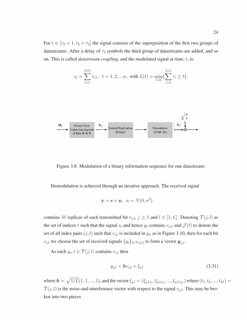
For each datastream, a binary information sequence, ul = u1,lu2,lu3,l, ..., uK,l, enters
a binary forward error correction encoder of rate R=K/N. Each bit of the encoded binary
sequence, vl = v1,lv2,lv3,l, ..., vN,l, with vj,l ∈ {−1, 1}, j = 1, 2, ..., N is replicated M
times and permuted producing a sequence, vl = v1,lv2,lv3,l, ..., vMN,l. The L modulated
datastreams are added together after certain chosen time offsets. The first group of datas-
treams starts at time t = 1, after τ2 intervals the second group of datastreams initiates.
1In the modulation format presented in Chapter 5 and 6, signature sequences are used for modulation,however, in the following modulation format this is not included
2For example, GMSK is used as a digital modulation approach for AIS.
24
For t ∈ [τ2 + 1, τ2 + τ3] the signal consists of the superposition of the first two groups of
datastreams. After a delay of τ3 symbols the third group of datastreams are added, and so
on. This is called datastream coupling, and the modulated signal at time, t, is:
st =
L(t)∑l=1
vt,l, t = 1, 2, ...w, with L(t) = minl>0
{l+1∑i=2
τi ≥ t}.
Figure 3.8: Modulation of a binary information sequence for one datastream.
Demodulation is achieved through an iterative approach. The received signal
y = s+ n, n ∼ N(0, σ2)
contains M replicas of each transmitted bit vj,l, j ≥ 1 and l ∈ [1, L]. Denoting T (j, l) as
the set of indices t such that the signal st and hence yt contains vj,l, and J (t) to denote the
set of all index pairs (j, l) such that vj,l is included in yt, as in Figure 3.10, then for each bit
vj,l we choose the set of received signals {yt}t∈T (j,l) to form a vector yj,l.
As each yt, t ∈ T (j, l) contains vj,l then
yj,l = hvj,l + ξj,l (3.31)
where h =√1/L(1, 1, ..., 1), and the vector ξj,l = (ξj,l,t1 , ξj,l,t2 , ..., ξj,l,tM ) where (t1, t2, ..., tM) =
T (j, l) is the noise-and-interference vector with respect to the signal vj,l. This may be bro-
ken into two pieces
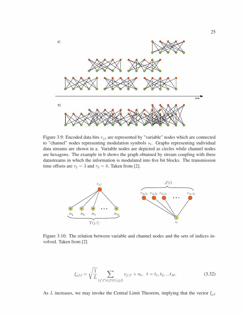
25
Figure 3.9: Encoded data bits vj,l are represented by "variable" nodes which are connectedto "channel" nodes representing modulation symbols st. Graphs representing individualdata streams are shown in a. Variable nodes are depicted as circles while channel nodesare hexagons. The example in b shows the graph obtained by stream coupling with threedatastreams in which the information is modulated into five bit blocks. The transmissiontime offsets are τ2 = 3 and τ3 = 8. Taken from [2].
Figure 3.10: The relation between variable and channel nodes and the sets of indices in-volved. Taken from [2]
ξj,l,t =
√1
L
∑(j′,l′)∈J (t)\(j,l)
vj′,l′ + nt, t = t1, t2, ...tM . (3.32)
As L increases, we may invoke the Central Limit Theorem, implying that the vector ξj,l
26
converges to a Gaussian random vector with independent zero-mean components and co-
variance matrix Rj,l = diag(σ2t1, σ2
t2, ...σ2
tM) where σ2
t denotes the variance of ξj,l,t. For
t > 2W + 1 the number of elements in the set J (t) is L and so the variance of σ2t =
(L − 1)/L + σ2 according to (3.32) When t ≤ 2W + 1, the size of the set J (t) is less
than L, and so the variances are influenced by the interference cancellation throughout the
demodulation iterations, the expression based on σ2t is preferred.
With this vector yj,l one may perform minimum mean-squared error (MMSE) filtering
to form a SNR-optimal linear estimate of vj,l given by
zj,l = wTj,lyj,l = wT
j,lhvj,l +wTj,lξj,l (3.33)
wTj,l = (I + h∗R−1
j,l h)−1h∗R−1
j,l . (3.34)
This minimizes ||wj,lyj,l − vj,l||2. The resulting SNR of the signal zj,l is then
γj,l = h∗R−1j,l h =
1
L
∑t∈T (j,l)
1
σ2t
(3.35)
As vj,l ∈ {1,−1}, and takes each of the two values with equal probability 1/2, one can
form a conditional expectation estimate vj,l of vj,l as
vj,l = E(vj,l|zj,l) = tanh(zj,lγj,l) = tanh
⎡⎣zj,l 1
L
∑t∈T (j,l)
1
σ2t
⎤⎦ (3.36)
With all of the estimates vj,l computed for all data bits vj,l j = 1, 2, ... and l ∈ [1, L]
the next iteration starts with interference cancellation performed by computing y(1)j,l with
components
y(1)j,l,t = yt −
√1
L
∑(j′,l′)∈J (t)\(j,l)
vj′,l′ , t ∈ T (j, l). (3.37)
27
From which we have the vector
y(1)j,l = hvj,l + ξ
(1)j,l (3.38)
with components of ξ(1)j,l
ξ(1)j,l,t =
√1
L
∑(j′,l′)∈J (t)\(j,l)
(vj′,l′ − vj′,l′) + nt, t ∈ T (j, l). (3.39)
This process continues by computing new estimates v(1)j,l by repeating the same procedure
to compute (3.34) and (3.36), and the estimation and interference cancellation steps are
repeated for a number of iterations. In order to avoid reusing the same information at each
iteration, one computes M extrinsic vectors y(i)j,l,t, t ∈ T (j, l) for each bit vj,l at iteration i
and the components of y(i)j,l,t are then
y(i)j,l,t′ = yt′ −
√1
L
∑(j′,l′)∈J (t)\(j,l)
v(i−1)j′,l′,t′
=
√1
Lvj,l +
√1
L
∑(j′,l′)∈J (t)\(j,l)
(vj′,l′ − v(t−1)j′,l′,t′) + nt′ (3.40)
where t′ �= t and t′ ∈ T (j, l). As before the vectors y(i)j,l,t are used to form M values for
z(i)j,l,t according to (3.34) and corresponding estimates v(i)j,l,t using (3.36) for each replication
of vj,l.
After a fixed number of iterations, I, the estimated bits are passed to a decoder to decode
the fowrward error correction codes used to encode the information into the datastreams.
Figure 3.11: General Structure of iterative demodulation prior to decoding.

28
As in the case of the LDPC codes, one can produce a recursive relation describing
the evolution of the noise-and-interference power. Assuming that the data block of MN
symbols consists of 2W +1 equal length subblocks, with time measured in subblocks, and
that the L datastreams are split into 2W+1 equal size groups. The analysis of the evolution
of the noise-and-interference power at iteration i for symbols vj,l transmitted at time t is
now:
xti =
1
2W + 1
W∑j=−W
gm
(1
α
1
2W + 1
W∑l=−W
1
xt+j+li−1
)+ σ2, (3.41)
where the function gm is given as
gm(a) = E[(1− tanh(a+ ζ√a))2], ζ ∼ N(0, 1)
and α is the modulation load.
Definition 3.5.1. The modulation load is the ratio of the number of users divided by the
number of replicas made for each message
α =L
M
Assuming that transmission starts at t = 1, and that at each instant, t, the modulation
load is increased by α/(2W + 1) for t ∈ [1, 2W + 1] the initial conditions are
xt0 = 0, t ≤ 0;
xt0 =t
2W+1 + σ2, t ∈ [1, 2W + 1]; (3.42)
xt0 = 1 + σ2, t > 2W + 1.
The system converges if equation (3.41) approaches some small value. Notice that
(3.41) resembles a SC system, where α acts as the ε parameter. However, to put this into
the appropriate form where x(∞) = 0 will be a fixed point, we must examine the fixed
points of the uncoupled case. Setting W = 0, we produce the recursion describing the
evolution of the noise-and-interference power during the demodulation iterations:
xi = gm
(1
αxi−1
)+ σ2. (3.43)
29
Depending on the choice of α this equation will have one, two, or three fixed points for
x ∈ [0,∞). In the case where (3.43) has three fixed points such that x(1) < x(2) < x(3).
The roots x(1) and x(3) will be stable, while x(2) will be an unstable fixed point.
Denoting the capacity of the AWGN channel with SNR 1/σ2 as
C(σ2) =1
2log2
(1 +
1
σ2
)(3.44)
we may provide upper and lower bounds on the stable roots where the proof is given in [2]:
Lemma 3.5.2. For σ2 ≤ 1, the following statements are satisfied:
1. for α ∈ [0, C(σ2)], σ2 ≤ x(1) ≤ (1 + e−1/σ)σ2 ≤ 2σ2,
2. for α ∈ [4, C(σ2)], 1 + σ2 − 2α≤ x(3) ≤ 1 + σ2,
3. for α ∈ [5, C(σ2)], x(3) = 1 + σ2 − 1α(1+σ2)
+ ρ(α, σ2) where ρ is bounded by a
function ρ(α) such that |ρ(α, σ2)| ≤ ρ(α) = o(1α
)for σ2 ∈ [0, 1],
4. for σ ≤ 0.01 and α ≥ 2, 0.3 ≤ x(3) ≤ 1 + σ2
With approximate neighbourhoods of each fixed point known, we introduce the following
functions:
f(x;α) = gm(1α
(1
x(1) − x))
+ σ2 − x(1),
g(x) = 1x(1) − 1
x(1)+x,
the recursion (3.41) may now be written as
xti =
1
2W + 1
W∑j=−W
f
(1
2W + 1
W∑l=−W
g(xt+j+li−1
);α
).
The potential function for the uncoupled case (W=0) is then
U(x;α) = ln
(x+ x(1)
x(1)
)− σ2x
x(1)(x+ x((1))− α
∫ 1
αx(1)
1
α(x+x(1))
gm(y)dy.
The convergence of this spatially coupled system has important implications for the
achievable rate and capacity of the signaling format [2]. If the system (3.41) converges
30
to its smallest root x(1) of (3.43) after I iterations, the SNR of the demodulated data bits
equals M/(Lx(1)) = 1/(αx(1)). Each replica suffers noise-and-interference power x(1),
and the replicas are added together. Thus, the total communication rate achievable by the
system will be
R(α, σ2) =L
MCBIAWGN
(M
Lx(1)
)= αCBIAWGN
(1
αx(1)
).
where CBIAWGN(a) denotes the capacity of the binary-input AWGN channel with SNR, a.
Letting α(σ2,W ) denote the maximum load for which the coupled system converges to
x(1) for a given σ2 and W the following theorem holds [2]:
Theorem 3.5.3. There exists a W > 0 such that ∀ W > W
R(α, σ2) = C(σ2)−3
2ln2
C(σ2)+ o
(1
C(σ2)
).
as σ2 → 0 and thus limσ2→0(C(σ2)−R(α, σ2)) = 0
3.5.2 MIMO Block Fading Channel
Consider a multi-user MIMO system, where K data streams are transmitted by L inde-
pendent users to a MIMO receiver with two receiving antennas. User l ∈ {1, 2, · · · , L}transmits a signal vector vl (single data stream). First a binary information sequence
ul = u1,l, u2,l, u3,l, · · · , uK,l enters a binary forward error correction encoder of rate R =
K/N . Then each bit of the encoded binary sequence vl = v1,l, v2,l, v3,l, · · · , vN,l, where
vj,l ∈ {1, 1} , j = 1, 2, · · · , N is replicated M times and permuted producing a sequence
vl = v1,l, v2,l, · · · , vMN,l. The power of each user is P/M . The signals y1 and y2 received
at the two receive antennas at time t are then
yt,1 =
√P
M
L∑i=1
h1,t,ivj,i + n1,t
yt,2 =
√P
M
L∑i=1
h2,t,ivj,i + n2,t
31
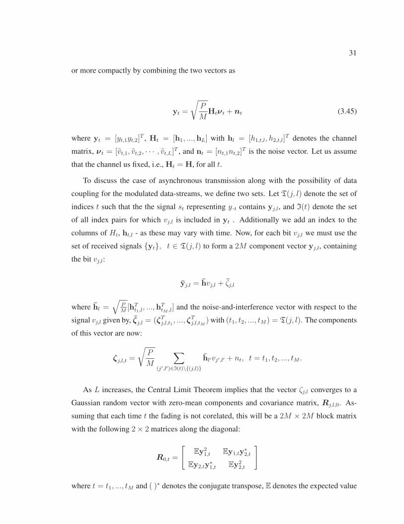
or more compactly by combining the two vectors as
yt =
√P
MHtνt + nt (3.45)
where yt = [yt,1yt,2]T , Ht = [h1, ...,hL] with hl = [h1,t,l, h2,t,l]
T denotes the channel
matrix, νt = [vt,1, vt,2, · · · , vt,L]T , and nt = [nt,1nt,2]T is the noise vector. Let us assume
that the channel us fixed, i.e., Ht = H, for all t.
To discuss the case of asynchronous transmission along with the possibility of data
coupling for the modulated data-streams, we define two sets. Let T(j, l) denote the set of
indices t such that the the signal st representing y.t contains yj,l, and I(t) denote the set
of all index pairs for which vj,l is included in yt . Additionally we add an index to the
columns of Ht, ht,l - as these may vary with time. Now, for each bit vj,l we must use the
set of received signals {yt}, t ∈ T(j, l) to form a 2M component vector yj,l, containing
the bit vj,l:
yj,l = hvj,l + ζj,l
where hl =√
PM[hT
t1,l, ...,hT
tM ,l] and the noise-and-interference vector with respect to the
signal vj,l given by, ζj,l = (ζTj,l,t1
, ..., ζTj,l,tM
) with (t1, t2, ..., tM) = T(j, l). The components
of this vector are now:
ζj,l,t =
√P
M
∑(j′,l′)∈I(t)\{(j,l)}
hl′vj′,l′ + nt, t = t1, t2, ..., tM .
As L increases, the Central Limit Theorem implies that the vector ζj,l converges to a
Gaussian random vector with zero-mean components and covariance matrix, Rj,l,0. As-
suming that each time t the fading is not corelated, this will be a 2M × 2M block matrix
with the following 2× 2 matrices along the diagonal:
R0,t =
[Ey2
1,t Ey1,ty∗2,t
Ey2,ty∗1,t Ey2
2,t
]
where t = t1, ..., tM and ( )∗ denotes the conjugate transpose, E denotes the expected value
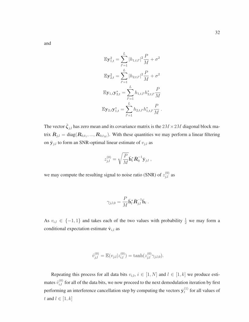
32
and
Ey21,t =
L∑l′=1
|h1,t,l′ |2P
M+ σ2
Ey22,t =
L∑l′=1
|h2,t,l′ |2P
M+ σ2
Ey1,ty∗2,t =
L∑l′=1
h1,t,l′h∗2,t,l′
P
M
Ey2,ty∗1,t =
L∑l′=1
h2,t,l′h∗1,t,l′
P
M.
The vector ζj,l has zero mean and its covariance matrix is the 2M×2M diagonal block ma-
trix Rj,l = diag(R0,t1 , ...,R0,tM ). With these quantities we may perform a linear filtering
on yj,l to form an SNR-optimal linear estimate of vj,l as
z(0)j,l =
√P
Mh∗l R
−10 yj,l ,
we may compute the resulting signal to noise ratio (SNR) of z(0)j,l as
γj,l,0 =P
Mh∗l R
−1j,l hl .
As vi,l ∈ {−1, 1} and takes each of the two values with probability 12
we may form a
conditional expectation estimate vi,l as
v(0)j,l = E(vj,l|z(0)i,l ) = tanh(z
(0)j,l γj,l,0).
Repeating this process for all data bits vi,l, i ∈ [1, N ] and l ∈ [1, k] we produce esti-
mates v(0)i,l for all of the data bits, we now proceed to the next demodulation iteration by first
performing an interference cancellation step by computing the vectors y(1)t for all values of
t and l ∈ [1, k]

33
y(1)j,l,t = yt −
∑(j′,l′)∈I(t)\{(j,l)}
hl′ v(0)j′,l′
√P
M
=
√P
Mhlvj,l +
√P
M
∑(j′,l′)∈I(t)\{(j,l)}
hl′(vj′,l′ − v(0)j,l′) + nt
=
√P
Mhlvj,l + ζ
(1)j,l
where ζ(1)j,l denotes the two-dimensional noise and interference vector for the bit vj,l at time
t for the first iteration.
In order to estimate a particular bit vj,l we collect M replicas of vj,l transmitted at times
t1, t2, · · · , tM to produce the 2M -vector y(1)j,l = [y
(1) Tt1 ,y
(1) Tt2 , · · · ,y(1) T
tM]T , and the 2M -
vector of the interference and noise ζ(1)j,l = [ζ
(1) Tt1 , ζ
(1) Tt2 , · · · , ζ(1) T
tM]T . This implies
y(1)j,l =
√P
Mhlvj,l + ζ
(1)j,l (3.46)
Again, for large values of L, the Central Limit Theorem implies that the vector ζ(1)j,l
converges to a Gaussian random vector with zero-mean components and covariance matrix,
Rj,l,1, which is a block diagonal matrix with 2× 2 block matrices:
R1,t =
[Ey
(1) 21,t Ey
(1)1,ty
(1)∗2,t
Ey(1)2,ty
(1)∗1,t Ey
(1) 22,t
]
Denoting σ2mmse,l,0 = E[1 − tanh(z
(0)j,l γl,0)] the components of the new covariance matrix
34
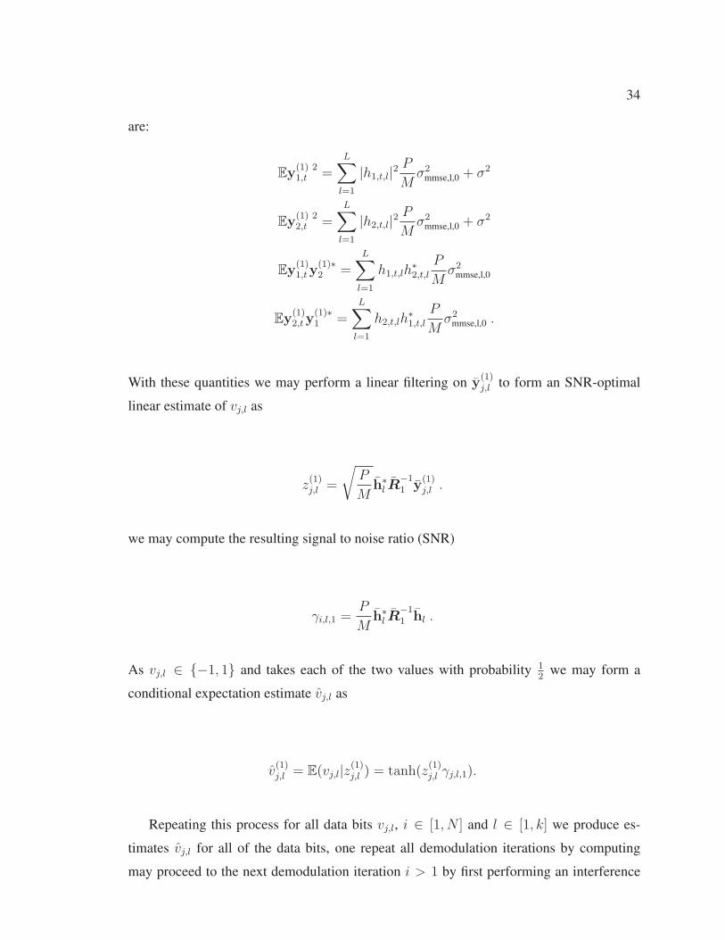
are:
Ey(1) 21,t =
L∑l=1
|h1,t,l|2P
Mσ2
mmse,l,0 + σ2
Ey(1) 22,t =
L∑l=1
|h2,t,l|2P
Mσ2
mmse,l,0 + σ2
Ey(1)1,ty
(1)∗2 =
L∑l=1
h1,t,lh∗2,t,l
P
Mσ2
mmse,l,0
Ey(1)2,ty
(1)∗1 =
L∑l=1
h2,t,lh∗1,t,l
P
Mσ2
mmse,l,0 .
With these quantities we may perform a linear filtering on y(1)j,l to form an SNR-optimal
linear estimate of vj,l as
z(1)j,l =
√P
Mh∗l R
−11 y
(1)j,l .
we may compute the resulting signal to noise ratio (SNR)
γi,l,1 =P
Mh∗l R
−11 hl .
As vj,l ∈ {−1, 1} and takes each of the two values with probability 12
we may form a
conditional expectation estimate vj,l as
v(1)j,l = E(vj,l|z(1)j,l ) = tanh(z
(1)j,l γj,l,1).
Repeating this process for all data bits vj,l, i ∈ [1, N ] and l ∈ [1, k] we produce es-
timates vj,l for all of the data bits, one repeat all demodulation iterations by computing
may proceed to the next demodulation iteration i > 1 by first performing an interference
35
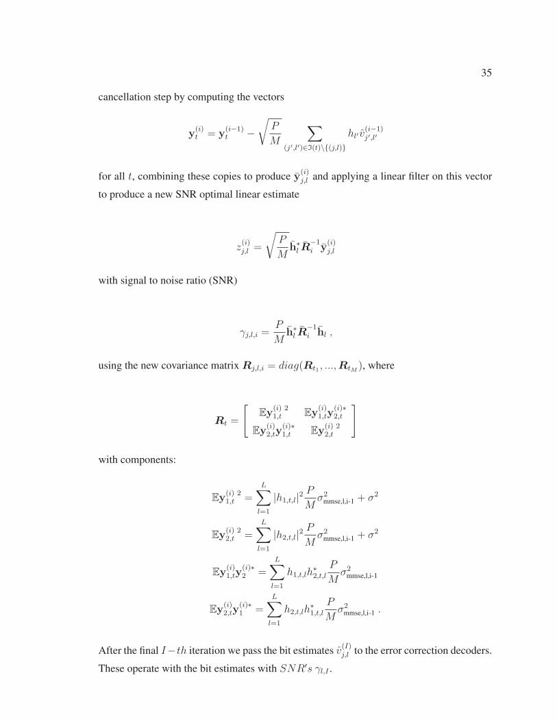
cancellation step by computing the vectors
y(i)t = y
(i−1)t −
√P
M
∑(j′,l′)∈I(t)\{(j,l)}
hl′ v(i−1)j′,l′
for all t, combining these copies to produce y(i)j,l and applying a linear filter on this vector
to produce a new SNR optimal linear estimate
z(i)j,l =
√P
Mh∗l R
−1i y
(i)j,l
with signal to noise ratio (SNR)
γj,l,i =P
Mh∗l R
−1i hl ,
using the new covariance matrix Rj,l,i = diag(Rt1 , ...,RtM ), where
Rt =
[Ey
(i) 21,t Ey
(i)1,ty
(i)∗2,t
Ey(i)2,ty
(i)∗1,t Ey
(i) 22,t
]
with components:
Ey(i) 21,t =
L∑l=1
|h1,t,l|2P
Mσ2
mmse,l,i-1 + σ2
Ey(i) 22,t =
L∑l=1
|h2,t,l|2P
Mσ2
mmse,l,i-1 + σ2
Ey(i)1,ty
(i)∗2 =
L∑l=1
h1,t,lh∗2,t,l
P
Mσ2
mmse,l,i-1
Ey(i)2,ty
(i)∗1 =
L∑l=1
h2,t,lh∗1,t,l
P
Mσ2
mmse,l,i-1 .
After the final I−th iteration we pass the bit estimates v(I)j,l to the error correction decoders.
These operate with the bit estimates with SNR′s γl,I .

36
This demodulation approach produces a similar recursion equation, however it is now
a vector recursion. This vector recursion is not conservative and so a Lyapunov potential
function cannot be determined to study its threshold saturation behaviour.
Chapter 4
Compressed Sensing Using Message Passing
4.1 Introduction
The recovery of an unknown high-dimensional sparse signal based on a collection of
noisy measurements has been studied extensively in the past decade [28, 29, 30, 31, 32,
33]. The interest in estimation problems with sparsity constraints arises from the potential
applications in signal processing, such as denoising, compression and sampling [34, 35,
36, 37, 38]. The original compressed sensing problem considered noisy measurements of a
deterministic vector, and it is assumed that x0 has a sparse representation x0 = Dα0 where
D is a given dictionary and the majority of the entries of α0 are zero.
This permits the representation of x0 as a linear combination of a small number of
"atoms" or columns of D. Thus the goal of any estimation technique is to recover either
x0 or its sparse representation given by α0. There are several practical approaches to this
problem, these include �1 relaxation methods such as the Dantzig selector [33], Basis pur-
suit denoising (BPDN) which is also known as the Lasso. [28, 29, 39]. These approaches
rely on methods from linear programming (LP), and these approaches can be substantially
more expensive in applications than the standard linear reconstruction schemes. As an
alternative one can consider iterative algorithms that achieve reconstruction performance
comparable to the LP-based approaches while running considerably faster. Examples of
these are greedy algorithms such as thresholding and orthogonal matching pursuit (OMP)
[40], and implementations of message passing.
Several authors have approached compressed sensing from the information-theoretic
perspective [41, 42, 43, 44]. Notably Wu and Verdu presented information-theoretic lower
bounds on the undersampling rate in terms of Rényi information dimensions of the esti-
mated vector for noiseless [43] and noisy sensing [44] cases. This has allowed for com-
pressed sensing to be considered for vectors with components drawn from a given set based
on some probability distribution which allows one to drop the sparseness requirement on
the input vector. The connection between achievable compressed sensing undersampling
37
38
rates and multi-user efficients were computed using methods from statistical mechanics
[44, 45].
In [46] it is shown that a special construction of band-diagonal sensing matrices built
from random Gaussian matrices and the AMP algorithm have been used to approach the
ultimate reconstruction limits according to Rényi information dimension. In terms of ex-
panding the achievable limits of the reconstruction, spatial graph coupling has made sig-
nificant progress. It has been shown by Kudekar and Pfister [47], and Krzakala et. al. [48]
that coupled sensing matrices can be used efficiently for compressed sensing.
4.2 Sparse Estimation Problems
In this section we describe two common estimation problems. Wherein the unknown
parameter has a sparse representation with respect to a known dictionary. A measurement
of the unknown deterministic signal x0 ∈ Rn is given by y ∈ R
m
y = Ax0 +w (4.1)
where w is an independent, identically distributed (IID) Gaussian noise with zero mean and
variance σ2, and A is a known m× n matrix. We require that A is non-adaptive, implying
that measurements do not depend on measurements made previously.
It is assumed as prior knowledge that there exists a sparse representation of x0, i.e.,
x0 ∈ S = {x ∈ Rn : x = Dα, ||α||0 ≤ s}. (4.2)
The set S describes signals x which can be formed from linear combinations of s columns
from D (commonly called atoms). The dictionary D is a known n × p matrix with n ≤ p,
and it is further assumed that s < p to ensure only a subset of atoms in D can be used to
represent any signal in S, and that this number s is known.
As an example, in [16] the authors consider three possible compressed sensing prob-
lems which are similar to (4.1) with potentially Gaussian random matrices A and informa-
tion vectors of three types:
� Sparse vectors with non-negative entries.
� Sparse vectors with signed components.
39
� Vectors with components xi ∈ [−1, 1] and at most k � n entries with values in the
interior (−1, 1).
Given such a measurement, the goal is to obtain an estimate x whose average mean
squared error (MSE),
MSE = E[||x− x0||22] (4.3)
is as small as possible. As x0 is deterministic, the expectation above is taken over the noise
of w, but not x0, and so we may treat this as a function of x0.
It may also be of interest to estimate the coefficient vector α0 for which x0 = Dα0,
say for the purpose of model selection [28, 33]. In such a scenario, one must construct
an estimator α whose MSE, E[||α − α0||22] is as low as possible. Unless D is unitary,
estimating α0 is not equivalent to estimating x0. Of course when estimating for α0 we may
combine the two matrices to produce an equivalent problem
y = Hα0 +w (4.4)
where H = AD is an m× p matrix and
α0 ∈ T = {α ∈ Rp : ||α0||0 ≤ s}. (4.5)
This is just a special case of (4.1) and (4.2) with the p-dimensional identity matrix acting
as D in (4.2). Signal estimation problems differ in the properties of the dictionary D
and measurement matrix A. For example, distinctly different problems arise depending on
whether the dictionary is a basis or an over-complete frame.
Alternatively, in accordance with the results [43, 44, 45] one can drop the requirement
that x is sparse and instead consider vectors with components as random variables with
some probability distribution. In this work we consider the sensing problem
y = Ax0 +w
where x with entries arising from the binomial distribution, w is a noise vector as stated in
(4.1), and A is a band-diagonal sparse m× n matrix.

40
4.3 Inference from Message Passing
We have considered linear measurement problems of the form [49]
y = Ax+w
where A is a known measurement matrix and w a noise vector. The graphical model ap-
proach to reconstructing the original vector x is to postulate a joint probability distribution
on the transmitted and received vectors which is of the form
p(dx, dy) = p(dy|x)p(dx) (4.6)
The conditional distribution p(dy|x) models the noise process, while the prior p(dx) en-
codes information on the vector. In compressed sensing this can describe its sparsity prop-
erties. Either of these distributions (or both) is factorized according to a specific graph
structure, and the resulting posterior distribution p(dy|x) can be used to infer x given y.
To illustrate this, we consider the conditional distribution of y given x which is equiv-
alent to specifying the distribution of the noise vector w. We will assume that p(w) is
Gaussian with zero mean and variance β−1I , and so
pβ(dy|x) =(
β
2π
)n2
exp(−β
2||y −Ax||22
)dy (4.7)
For the prior p(dx) we use the product distribution with identical factors.
The posterior distribution of x given observations y admits an explicit expression de-
rived from pβ(dx, dy)
pβ(dy|y) =(
β
2π
)n2 1
p(y)exp(−β
2||y −Ax||22
)dyΠn
i=1p(dxi). (4.8)
Despite this explicit expression, computing marginals or expectations of this distribution is
computationally hard.

41
Notice that the square residuals ||y−Ax||22 decompose into a sum of m terms, produc-
ing a simpler expression
pβ(dy|y) =(
β
2π
)n2 1
p(y)Πm
a=1exp(−β
2(ya − (Ax)a)
2
)dyΠn
i=1p(dxi). (4.9)
where (Ax)a is the a−th entry of the vector Ax. This factorized structure can be expressed
as bipartite graph including a "variable node" i ∈ [1, n] for each variable xi and a "factor
node" a ∈ [1,m] for each term Ψa(x) = exp(−β
2(ya − (Ax)a)
2)
Variable i and factor a
are connected by an edge if and only if Ψa(x) depends non-trivially on xi (i.e., Aai �= 0).
We will call such a bipartite graph, a factor graph.
Figure 4.1: Factor graph associated to the probability distribution (4.9). Circles correspondto variables xi, i ∈ [1, n] and squares correspond to measurements ya, a ∈ [1,m].
An estimate of the signal can be extracted from the posterior distribution in several
ways. One could use the conditional expectation
xβ(y; p) =
∫Rn
xpβ(dy|x), (4.10)
this estimate achieves the minimal mean square error if pβ(dx, dy) is the actual joint dis-
tribution of the problem. In practical terms, this estimator is hard to compute. To pro-
duce something more tractable, we suppose that p(dxi) = pβ,h(dxi) = cfβ,h(xi)dxi for
fβ,h(xi) = e−βh(xi) an un-normalized probability density function. As β becomes large,
the integral (4.10) becomes dominated by the vector x with the highest posterior probabil-
ity pβ and one can replace the integral in dx with a maximization over x and define the
following minimization over a cost function CA,y(z;h),
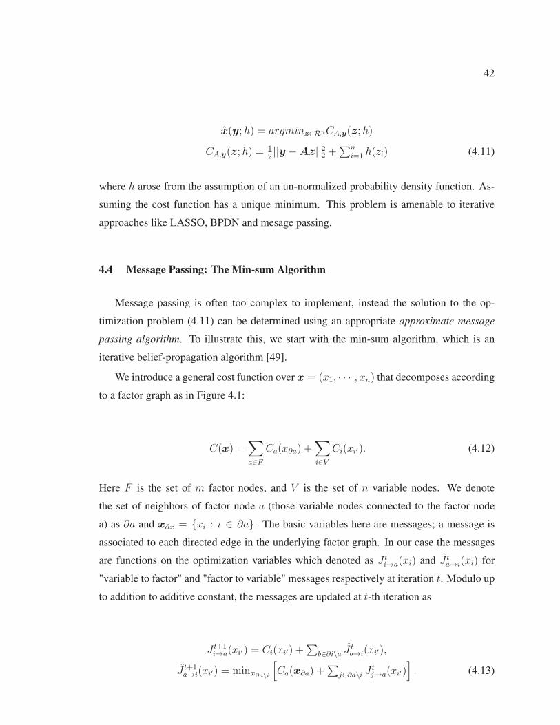
42
x(y;h) = argminz∈RnCA,y(z;h)
CA,y(z;h) =12||y −Az||22 +
∑ni=1 h(zi) (4.11)
where h arose from the assumption of an un-normalized probability density function. As-
suming the cost function has a unique minimum. This problem is amenable to iterative
approaches like LASSO, BPDN and mesage passing.
4.4 Message Passing: The Min-sum Algorithm
Message passing is often too complex to implement, instead the solution to the op-
timization problem (4.11) can be determined using an appropriate approximate message
passing algorithm. To illustrate this, we start with the min-sum algorithm, which is an
iterative belief-propagation algorithm [49].
We introduce a general cost function over x = (x1, · · · , xn) that decomposes according
to a factor graph as in Figure 4.1:
C(x) =∑a∈F
Ca(x∂a) +∑i∈V
Ci(xi′). (4.12)
Here F is the set of m factor nodes, and V is the set of n variable nodes. We denote
the set of neighbors of factor node a (those variable nodes connected to the factor node
a) as ∂a and x∂x = {xi : i ∈ ∂a}. The basic variables here are messages; a message is
associated to each directed edge in the underlying factor graph. In our case the messages
are functions on the optimization variables which denoted as J ti→a(xi) and J t
a→i(xi) for
"variable to factor" and "factor to variable" messages respectively at iteration t. Modulo up
to addition to additive constant, the messages are updated at t-th iteration as
J t+1i→a(xi′) = Ci(xi′) +
∑b∈∂i\a J
tb→i(xi′),
J t+1a→i(xi′) = minx∂a\i
[Ca(x∂a) +
∑j∈∂a\i J
tj→a(xi′)
]. (4.13)
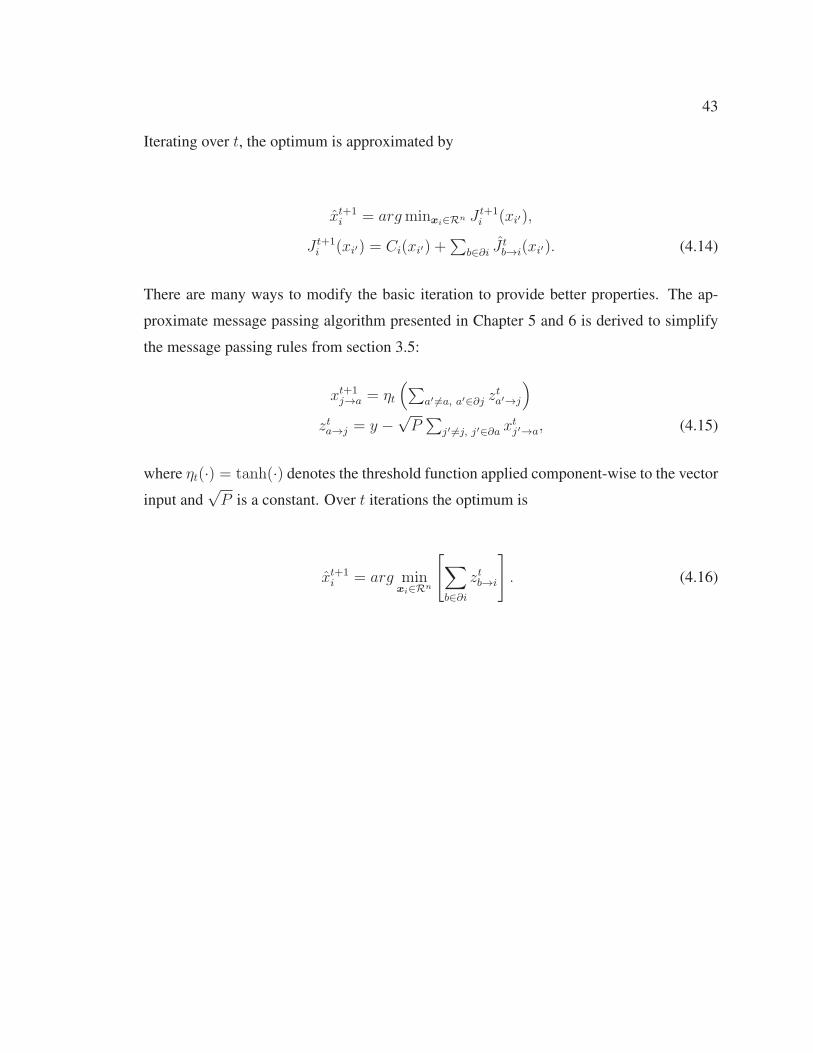
43
Iterating over t, the optimum is approximated by
xt+1i = argminxi∈Rn J t+1
i (xi′),
J t+1i (xi′) = Ci(xi′) +
∑b∈∂i J
tb→i(xi′). (4.14)
There are many ways to modify the basic iteration to provide better properties. The ap-
proximate message passing algorithm presented in Chapter 5 and 6 is derived to simplify
the message passing rules from section 3.5:
xt+1j→a = ηt
(∑a′ �=a, a′∈∂j z
ta′→j
)zta→j = y −
√P∑
j′ �=j, j′∈∂a xtj′→a, (4.15)
where ηt(·) = tanh(·) denotes the threshold function applied component-wise to the vector
input and√P is a constant. Over t iterations the optimum is
xt+1i = arg min
xi∈Rn
[∑b∈∂i
ztb→i
]. (4.16)
Chapter 5
Coupling Information Transmission with
Approximate Message Passing
In this section we focus on the coupling information transmission multi-user commu-
nication technique based on the spatial graph coupling principle [3] where the packets
transmitted from their respective datastreams have perfect timing. Each user transmits one
or more independently encoded data streams over the multiple access channel.
Each data stream is encoded and modulated such that the relations between the data
bits and modulation symbols within each transmitted stream are represented by a bipartite
graph. The data streams are transmitted with time offsets enabling coupling of the transmit-
ted graphs into a single continuous graph chain at the receiver. The receiver performs iter-
ative message-passing interference cancellation and data estimation on the received graph
chain, followed by individual error-correction decoding, performed for each data stream
individually, providing near-capacity operation [2, 11].
Modulation of each data stream is accomplished with repetition, permutation, and
spreading of data. We start with an introduction to the coupling information transmission
system and present its compressed sensing representation in Section 5.1, we formulate the
AMP-based demodulation algorithm in Section 5.3, and give the derivation of the algorithm
in the Appendix. Simulation results and conclusions are given in Section 5.4.
In terms of expanding the achievable limits of the reconstruction, spatial graph cou-
pling has made significant progress. It has been shown by Kudekar and Pfister [47], and
Krzakala et. al. [48] that coupled sensing matrices can be used efficiently for compressed
sensing. We consider a demodulation technique based on approximate message passing
(AMP) proposed by Donoho et al. [16] for compressed sensing problems, and construct a
version of the AMP which is specially derived for our multi-user situation.
We start with an introduction to the coupling information transmission system and
present its compressed sensing representation in Section 5.1, we formulate the AMP-based
44

45
demodulation algorithm in Section 5.3, and give the derivation of the algorithm in the Ap-
pendix. Simulation results and conclusions are given in Section 5.4.
5.1 System Model
We consider a communication scenario where a number of distinct transmitters send
independently encoded and modulated streams of data to the common receiver. The en-
coding format follows the coupling data transmission technique outlined in [11][2]. Each
data stream � = 1, 2, 3, · · · is encoded and modulated as shown in Fig. 5.1. First, a binary
information sequence u� = u1,�, u2,�, · · · , uK,�, where uj,� ∈ {−1, 1} is encoded with a
binary error correction code of rate R = K/N to produce an N bit codeword v�.
Each bit vj,� ∈ {−1, 1}, j = 1, 2, · · · , N of v�, is then replicated M times. The
resulting sequence is permuted using a binary permutation matrix P � and bitwise mul-
tiplied with a pseudo-random binary signature sequence specific to data stream �, s� =
s1,�, s2,�, · · · , sMN,�, with sj,� ∈ {−1, 1}, producing a sequence v� = v1,�, · · · , vMN,�. The
resulting binary phase shift keying (BPSK) signal v� is multiplied by an amplitude√
P�/M
and transmitted over the Gaussian multiple access channel (see Fig. 5.1). The bit error rates
(BER) are computed assuming error-correction codes which are capacity achieving on a
binary-input Gaussian channel given post detection SNR. Thus the goal for demodulation
is to reduce the SNR to an acceptable threshold in order to pass to the error-correction
codes.
The encoding and modulation of the vector v� can be represented using matrix notation
as
√P�
Mv� =
√P�
MS�P �Rv� = B�v� (5.1)
where R is the MN ×N band-diagonal repetition matrix with M ones in each row, P � is
an MN ×MN permutation matrix, and S� = diag(s�) is an MN ×MN diagonal matrix
that has the signature sequence s� on its diagonal.
We focus on a transmission scenario where k modulated data streams are transmitted
over the channel with time offsets of θ1 ≤ θ2 ≤ θ3 ≤ · · · ≤ θk symbol (chip) durations.1
1Without loss of generality we assume that the received data streams are chip synchronized. Processingof fractional offsets is discussed in Section 5.3.
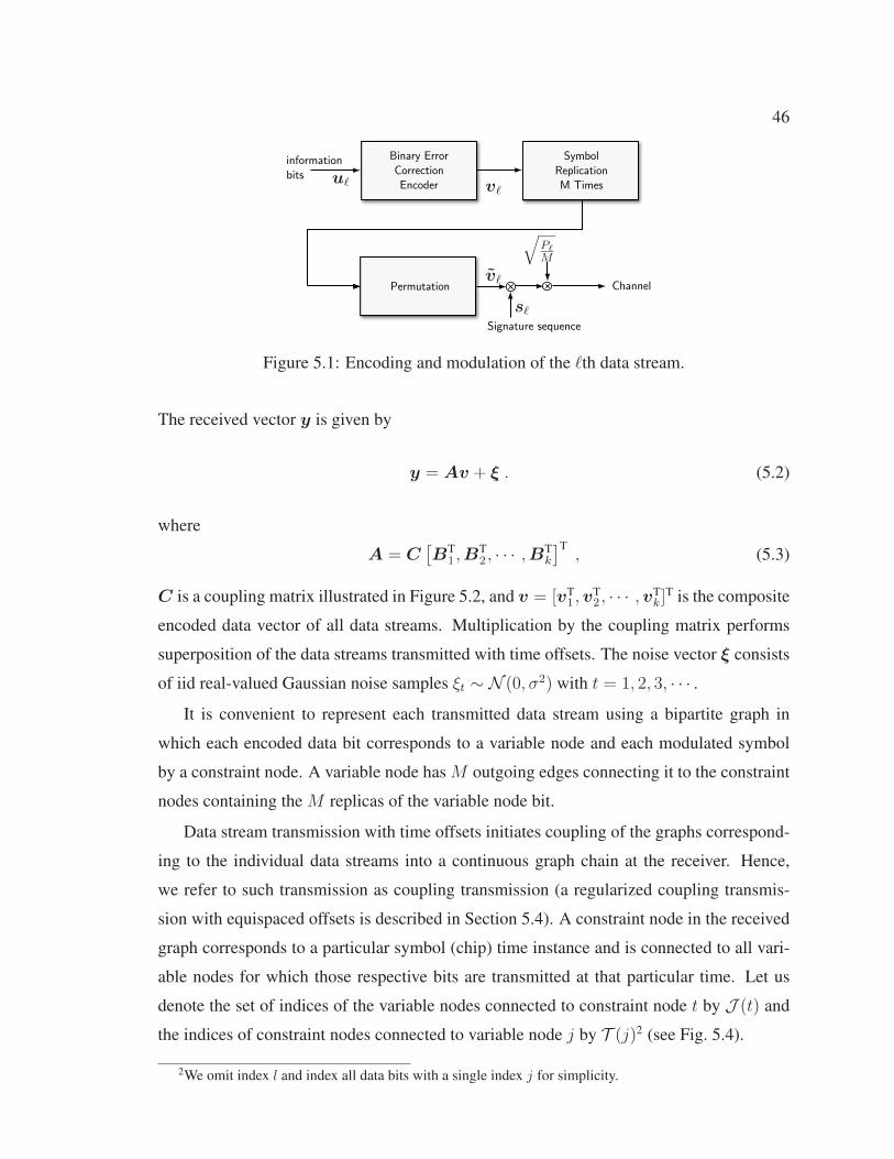
46
√P�M
s�
v�
v�u�
Signature sequence
Channel
informationbits
v
Binary Error Correction Encoder
Symbol ReplicationM Times
vPermutation
Figure 5.1: Encoding and modulation of the �th data stream.
The received vector y is given by
y = Av + ξ . (5.2)
where
A = C[BT
1 ,BT2 , · · · ,BT
k
]T, (5.3)
C is a coupling matrix illustrated in Figure 5.2, and v = [vT1 ,v
T2 , · · · ,vT
k]T is the composite
encoded data vector of all data streams. Multiplication by the coupling matrix performs
superposition of the data streams transmitted with time offsets. The noise vector ξ consists
of iid real-valued Gaussian noise samples ξt ∼ N (0, σ2) with t = 1, 2, 3, · · · .
It is convenient to represent each transmitted data stream using a bipartite graph in
which each encoded data bit corresponds to a variable node and each modulated symbol
by a constraint node. A variable node has M outgoing edges connecting it to the constraint
nodes containing the M replicas of the variable node bit.
Data stream transmission with time offsets initiates coupling of the graphs correspond-
ing to the individual data streams into a continuous graph chain at the receiver. Hence,
we refer to such transmission as coupling transmission (a regularized coupling transmis-
sion with equispaced offsets is described in Section 5.4). A constraint node in the received
graph corresponds to a particular symbol (chip) time instance and is connected to all vari-
able nodes for which those respective bits are transmitted at that particular time. Let us
denote the set of indices of the variable nodes connected to constraint node t by J (t) and
the indices of constraint nodes connected to variable node j by T (j)2 (see Fig. 5.4).
2We omit index l and index all data bits with a single index j for simplicity.

47
C =
θ1
θ2θ3θ4...
INM
INMINM
INM
INM
INMINM
INM
Figure 5.2: The MN × MN coupling matrix C consists of identity matrices surroundedby zeros. Each identity matrix IMN corresponds to an incoming data stream and its rowoffset corresponds to the time offset (starting time) of that data stream.
The alternative “compressed sensing” representation of the system is based on the
sparse m×n matrix A (see (5.2)). Note that the non-zero elements in row t, t = 1, 2, · · · ,mof A are indexed by the set J (t) and represent the indices of the data bits vj that are trans-
mitted at time t. The non-zero elements in a column j, j = 1, 2, · · · , n, of A represent
times at which a particular bit vj is transmitted over the channel and are indexed by the set
T (j).
5.2 Demodulation and Decoding
The receiver starts with joint iterative demodulation (multi-user detection) of the data
streams. At each iteration of the iterative demodulation process each bit vj is estimated
based on the M received symbols that contain the M transmitted replicas of vj ( bit estima-
tion stage). The estimated bits are then utilized to remodulate the data streams and perform
interference cancellation (interference cancellation stage). After the interference cancella-
tion stage the data streams are again passed to the bit estimation stage and the process is
repeated for a number of iterations until most of the inter-stream interference is removed.
The individual error correction decoding of the data streams is performed after the
final demodulation iteration. The decoding is not included into the demodulation loop to
simplify the system implementation and reduce the computational complexity. The system
is still capacity achieving asymptotically [11][2].
The iterative demodulation process can also be seen as message-passing on the system’s
graph chain. The interference cancellation message zit→j from constraint node t to variable
node j at demodulation iteration i and the bit estimation message back from node t to node

48
j at demodulation iteration i+ 1 are given by
zit→j = yt −∑
j′ �=j, j′∈J (t)
Atj′vij′→t (5.4)
vi+1j→t = tanh
⎛⎝ ∑
t′∈T (j),t′ �=t
At′jzit′→j
σ2,it′
⎞⎠ , (5.5)
where σ2,it is the noise and interference power experienced by the tth symbol of the re-
ceived signal at demodulation iteration i (see Fig. 5.4). The bit estimation performs maxi-
mum ratio combining over all signals zit→j containing bit vj and then takes the conditional
expectation estimate (see [11]). The interference cancellation step features subtraction of
all data streams except stream j from the received signal.
The number of messages computed, stored, and transmitted at each iteration of the
message-passing based iterative demodulation scales with the total number of the data bits
as well as the repetition factor M . An implementation, besides the main iteration loop,
requires a loop involving the exclusion of one message t′ = t or j′ = j.
y
y(i)l
x(i)l
yv(I)1
v(I)2
v(I)l∈L
Lpack(i)
. . .
. . .I iterationsInterference
CancellationData
Estimation
Error Correction Decoder 1
Error Correction Decoder 2
Lpacp k((i))Error Correction Decoder . . .
Figure 5.3: Diagram of the iterative receiver, with error correction decoding for each datastream.
5.3 The Proposed AMP-Based Demodulation Algorithm
Let vi denote an estimate of the entire data vector v computed at iteration i and zi
denote the residual noise and interference between the data streams at iteration i. The

49
j j′
tt′
J (t)
T (j)
zit→j′
vi+1j→t′
Figure 5.4: Graph representation of the modulated data.
proposed algorithms steps are as follows:
zi = y −Avi +zi−1
σ2,i−1◦ (A2 sech2(wi−1)), (5.6)
wi = AT zi
σ2,i+AT
2
1
σ2,i◦ vi . (5.7)
vi+1 = tanh(wi) (5.8)
where ◦ denotes the Hadamard (component-wise) product, A2 = A ◦ A and ’sech’ is the
hyperbolic secant function. The derivation of the algorithm is given in Appendix. The
initialization is done using
z0 = y, v0 = 0 . (5.9)
and σ2,i is computed from the variance of the residual zi.
The algorithm description is almost as compact and simple as linear multiuser detection
for CDMA such as a mean squared error (MSE) detector with just an addition of two
correction terms but without matrix inversions. Moreover, since matrix A is sparse, the
complexity of the actual matrix multiplication scale only with the number of non-zero
matrix entries. The role of the coupling matrix C to add data streams with time offsets,
and therefore, the operation Av can be performed as addition of the vectors B�v� with
offsets θ�. The number of operations performed per iteration scales only with the number
of data bits or received chips (which differ by the systems load factor). The implementation
requires a single iterative loop.
Finally, in the case that the time offsets θ1, θ2, · · · are not precisely chip time syn-
chronous the interference cancellation operation in (5.6) can be performed on sample basis.

50
SNR = Pα/σ2I [dB]
0 5 10 15 20 250
0.5
1
1.5
2
2.5
3
3.5
Rsum [bits/s/Hz]
Figure 5.5: Simulated coupling data transmission with AMP demodulation for M = 250(solid circles), M = 100 (dashed circles), full message-passing M = 250 (dotted squares),capacity of the GMAC channel (solid curve).
5.4 Numerical Results
The proposed algorithm can be applied in the case of arbitrary data stream transmission
offsets θ1, θ2, · · · . We present numerical results for a regularized offset scenario in which
the system is asymptotically capacity achieving [2]. Let us define a coupling parameter W
and assume that each packet consists of 2W + 1 sections of length ηW = MN/(2W + 1)
bits, where MN is divisible by 2W + 1. We then assume that data streams are transmitted
in groups of Lw where Lw is a parameter determining the system load α = Lw(2W+1)/M .
The time offsets are multiples of ηW , i.e. θ1 = θ2 = · · · = θLw = 0, θLw+1 = θLw+2 =
· · · = θ2Lw = ηW and so on, θj = ηW �j/Lw�. Small random deviations from this time
offsets will not influence the results.
Fig. 5.5 demonstrates simulated achievable sum rate of the coupling transmission with
the proposed AMP algorithm. We consider coupling window size W = 12, code length
N = 250 and focus on the case of equal power streams, P1 = P2 = · · · = P , known
to be the hardest for multi-user detection at high system loads. AMP demodulation with
repetitions factors M = 250 and M = 100 and given by the solid and dashed circle curves
respectively. The dotted squares curve represents full message passing for M = 250.
The rates are computed assuming error-correction codes which are capacity achieving on
a binary-input Gaussian channel given post detection SNR. The solid curve represents the
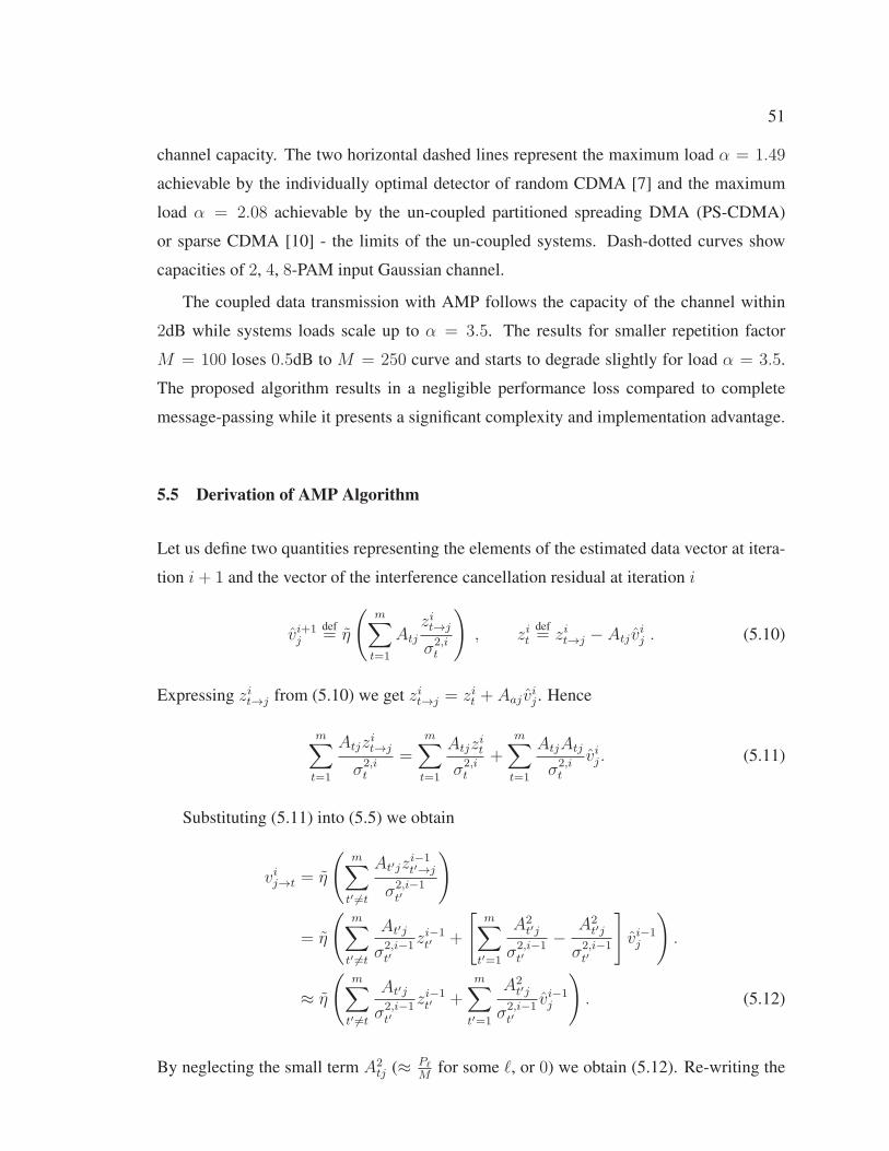
51
channel capacity. The two horizontal dashed lines represent the maximum load α = 1.49
achievable by the individually optimal detector of random CDMA [7] and the maximum
load α = 2.08 achievable by the un-coupled partitioned spreading DMA (PS-CDMA)
or sparse CDMA [10] - the limits of the un-coupled systems. Dash-dotted curves show
capacities of 2, 4, 8-PAM input Gaussian channel.
The coupled data transmission with AMP follows the capacity of the channel within
2dB while systems loads scale up to α = 3.5. The results for smaller repetition factor
M = 100 loses 0.5dB to M = 250 curve and starts to degrade slightly for load α = 3.5.
The proposed algorithm results in a negligible performance loss compared to complete
message-passing while it presents a significant complexity and implementation advantage.
5.5 Derivation of AMP Algorithm
Let us define two quantities representing the elements of the estimated data vector at itera-
tion i+ 1 and the vector of the interference cancellation residual at iteration i
vi+1j
def= η
(m∑t=1
Atj
zit→j
σ2,it
), zit
def= zit→j − Atj v
ij . (5.10)
Expressing zit→j from (5.10) we get zit→j = zit + Aaj vij . Hence
m∑t=1
Atjzit→j
σ2,it
=m∑t=1
Atjzit
σ2,it
+m∑t=1
AtjAtj
σ2,it
vij. (5.11)
Substituting (5.11) into (5.5) we obtain
vij→t = η
(m∑t′ �=t
At′jzi−1t′→j
σ2,i−1t′
)
= η
(m∑t′ �=t
At′j
σ2,i−1t′
zi−1t′ +
[m∑
t′=1
A2t′j
σ2,i−1t′
−A2
t′j
σ2,i−1t′
]vi−1j
).
≈ η
(m∑t′ �=t
At′j
σ2,i−1t′
zi−1t′ +
m∑t′=1
A2t′j
σ2,i−1t′
vi−1j
). (5.12)
By neglecting the small term A2tj (≈ P�
Mfor some �, or 0) we obtain (5.12). Re-writing the
52
first term in (5.12) above leads to
vij→t = η
((AT zi−1
σ2,i−1
)j
− Atjzi−1t
σ2,i−1t
+m∑
t′=1
A2t′j
σ2,i−1t′
vi−1j
)
Taking a Taylor series expansion up to the linear term, we find
vij→t ≈ η
((AT zi−1
σ2,i−1+AT
2
1
σ2,t−1◦ vi−1
)j
)
− Atjzi−1t
σ2,i−1t
η′
((AT zi−1
σ2,i−1+AT
2
1
σ2,i−1◦ vi−1
)j
)(5.13)
where ◦ denotes the Hadamard (component-wise) product, A2 = A ◦ A, and AT denotes
the transpose of the matrix A
Let us define the vector
wi−1 def= AT zi−1
σ2,i−1+AT
2
1
σ2,i−1◦ vi−1 . (5.14)
We can now represent (5.13) as
vij→t ≈ vij −Atjz
i−1t
σ2,i−1t
η′(wi−1
j
)(5.15)
and we also have
vij = η(wi−1j ) . (5.16)
To compute zit we apply (5.15) to (5.10) and obtain
zit = yt −n∑
j �=j′Atj′v
ij′→t − Atj v
ij
= yt −n∑
j �=j′Atj′
(vij −
Atj′zi−1t
σ2,i−1t
η′(wi−1j′ )
)− Atj v
ij
= yt − (Avi)t +n∑
j′=1
A2tj′z
i−1t
σ2,i−1t
η′(wt−1j′ )−
A2tj
σ2,i−1t
η(wt−1j ).

53
Again we will drop A2tj ≈ P�
Mleaving the approximation
zit ≈(y −Avi +
zi−1
σ2,i−1◦ (A2η
′(wi−1))
)t
. (5.17)
Finally (5.17), (5.14), and (5.16) give the AMP algorithm.

Chapter 6
Joint Packet Detection and Decoding for Maritime Data Exchange
Systems
Random access communications is an important mechanism of accessing the commu-
nication channel resources in the upcoming VHF data exchange, VDES as was previously
mentioned in Chapter 2. In satellite uplink communications a large varying user (ves-
sel) population is accessing the channel and coordinated channel access will be difficult to
implement. At the same time is it important to allow as many vessels as possible to com-
municate and share channel resources efficiently. Hence, the present time-division based
random access mechanism may not be able to cater to the growing traffic demand. In
addition to ship-to-satellite requests for downlink data transfer, tracking, and emergency
messages, short message exchange between ships and ship-to-shore can also be efficiently
handled with random access. Often, vessels do not need to establish a link but just need to
send a single packet.
We consider an approach to random access at the physical layer that is based on tech-
niques for simultaneously receiving several packets originating from distinct transmitters.
In a random access setting such receiver needs to accomplish two tasks: detect the start
of each incoming packet (timing acquisition) and decode the packets. The latter typically
also involves cancellation of mutual interference between the packets. It has been observed
already in the 90s for the case of code-division multiple access that the detection task lim-
its the multi-packet reception (MPR) capabilities of a receiver [50][51]. Later it has been
shown [52][53] that joint detection and decoding can improve the MPR capability. It has
also been proved in [54] that for packets modulated using generalized modulation format
and for specific packet power distribution the detection results in a loss that amounts to a
small fraction of the channel capacity asymptotically.
We focus on a spread spectrum transmission system that uses a constant envelop mod-
ulation and a spread preamble as in VDES uplink option [18], suitable for a simple im-
plementation in a vessel transmitter. We propose an algorithm for packet encoding at the
54

55
transmitter and joint packet detection and decoding at the receiver. Due to the specific
encoding format, from a communications theoretic perspective we can represent each mes-
sage as a bi-partite graph relating the data bits and the transmitted modulated symbols. At
the receiver consecutively received interfering packet graphs couple into a chain of graphs.
Our proposed joint iterative preamble detection, interference cancellation and decoding al-
gorithm is based on the AMP technique [16] and operates on the received graph chain.
Numerical results demonstrate that incorporation of the preamble detection into the itera-
tive decoding loop leads to a relatively minor performance loss compared to the throughput
of the system with an a priori timing knowledge assumption. The total throughput follows
the capacity of the multiple access channel. We also demonstrate that packet loads as high
as 2.95 packets per packet length per spreading factor are achievable and that the presented
random access mechanism outperforms the existing random access techniques.
6.1 System Model
bl d √Pl
M
sl
vl
vlul Signature Sequence
Preamble Information
Bits
Symbol Replication
M Times
Channel
lth packet'sdata
cket s
Binary Error Correction Encoder
Symbol Replication
M TimesPermutation
Payload Preamble
Figure 6.1: Encoding and modulation of one data packet.
We consider a scenario when a number of users send their data packets to the common
receiver. The users send packets on demand at random times and create random traffic
at the receiver. We assume that all packets are of the same length, the total number of
packets transmitted within a frame is Lpack, and the ordered set of packet indices is Lpack =
(1, 2, · · · , Lpack). The bit error rates (BER) are computed assuming error-correction codes
which are capacity achieving on a binary-input Gaussian channel given post detection SNR.
Thus the goal for demodulation is to reduce the SNR to an acceptable threshold in order to
pass to the error-correction codes.
Each packet begins with a preamble that will be used for the packet’s timing acquisition.
56
The preamble is followed by a payload consisting of the modulated original data to be sent.
To produce the payload of packet l ∈ Lpack a transmitter starts with encoding the binary data
vector ul = u1,l, u2,l, · · · , uK,l with a binary error correction code of rate R = K/N . After
the encoding each bit of the encoded sequence vl = v1,l, v2,l, · · · , vN,l, vj,l ∈ {1,−1}, is
repeated M times and the resulting sequence is permuted using a permutation described
by a binary permutation matrix P l. Finally, the permuted sequence is multiplied bit-by-bit
by the binary pseudo-random signature sequence sl = s1,l, s2,l · · · , sMN,l, sj,l ∈ {1,−1},
to produce vl = v1,l, v2,l, · · · , vMN,l. The resulting binary phase shift keying signal is
multiplied by a factor√
Pl/M , where Pl is the transmit power, and is transmitted over the
channel (see Fig. 6.1) 1.
Hence, each data bit is spread with a spreading factor M and the resulting spread
symbols (chips) are permuted. The modulation format follows the coupling information
transmission modulation principle [11], [55], [56], [2] and also resembles interleave divi-
sion multiple access (IDMA) [14], partition-spreading code-division multiple access (PS-
CDMA) [9, 10], generalized modulation [13], and superposition modulation [15]. The
modulated signal can be represented as a sparse graph connecting variable nodes corre-
sponding to the data bits vj,l to the channel access nodes corresponding to the times at
which M replicas of vj,l are transmitted over the channel. By T (j, l) we denote the set
of times τ1, τ2, · · · , τM at which the modulated replicas of bit vj,l are transmitted over the
channel.
To help the receiver find the starting time of the packet each transmitter starts its packet
with a preamble. Besides its purpose for timing acquisition the preamble also carries in-
formation. The information may include the seed of the spreading code and permutation
used for modulating the packet’s payload. Typically this information is encoded by a strong
error correction code. Assume that the preamble of the lth packet contains an information
bearing bit sequence bl = b1,l, b2,l, · · · , bNp,l where Np is the length of the preamble in bits.
To modulate the preamble each bit of the sequence bl is repeated M times and the result-
ing sequence is multiplied bit-by-bit by a binary signature sequence d = d1, d2, · · · , dMNp
to produce the preamble sequence bl = b1,l, b2,l, · · · , bMNp . The signature sequence d is
common to all preambles of all packets. As with the payload, the sequence bl is finally
1To simplify the presentation of the material we consider BPSK modulated packets. The format can beextended to QPSK modulation in a straightforward manner (see [54]).
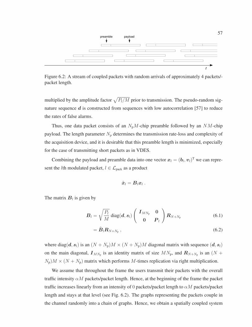
57
t
preamble payload
Figure 6.2: A stream of coupled packets with random arrivals of approximately 4 packets/-packet length.
multiplied by the amplitude factor√
Pl/M prior to transmission. The pseudo-random sig-
nature sequence d is constructed from sequences with low autocorrelation [57] to reduce
the rates of false alarms.
Thus, one data packet consists of an NpM -chip preamble followed by an NM -chip
payload. The length parameter Np determines the transmission rate-loss and complexity of
the acquisition device, and it is desirable that this preamble length is minimized, especially
for the case of transmitting short packets as in VDES.
Combining the payload and preamble data into one vector xl = (bl,vl)T we can repre-
sent the lth modulated packet, l ∈ Lpack as a product
xl = Blxl .
The matrix Bl is given by
Bl =
√Pl
Mdiag(d, sl)
(IMNp 0
0 P l
)RN+Np (6.1)
= BlRN+Np , (6.2)
where diag(d, sl) is an (N +Np)M × (N +Np)M diagonal matrix with sequence (d, sl)
on the main diagonal, IMNp is an identity matrix of size MNp, and RN+Np is an (N +
Np)M × (N +Np) matrix which performs M -times replication via right multiplication.
We assume that throughout the frame the users transmit their packets with the overall
traffic intensity αM packets/packet length. Hence, at the beginning of the frame the packet
traffic increases linearly from an intensity of 0 packets/packet length to αM packets/packet
length and stays at that level (see Fig. 6.2). The graphs representing the packets couple in
the channel randomly into a chain of graphs. Hence, we obtain a spatially coupled system
58
on which we will try to exhibit the threshold saturation phenomenon [5][6] via an iterative
message-passing-like receiver processing. The fact that the inter-packet interference grad-
ually increases at the beginning of the frame will help to start the detection and decoding
process which will then continue successfully for the duration of the entire frame.
We consider communication over the additive white Gaussian noise (AWGN) channel,
and so, the received signal y = (y1, y2, y3, ...) is computed as a superposition:
yτ =
L(τ)∑l=1
xτ,l + nτ , τ = 0, 1, 2, · · ·
where L(τ) denotes the number of interfering packets at time τ and nτ ∼ N (0, σ2) are the
iid noise samples.2 The received signal also allows for representation
y = ALpackx+ n , (6.3)
where x = (xT1 ,x
T2 , · · · ,xT
Lpack)T is the vector of stacked data and preamble information of
all packets, n is the vector of noise samples and
ALpack = CLpack
⎛⎜⎜⎜⎜⎜⎝
B1
B2
...
BLpack
⎞⎟⎟⎟⎟⎟⎠ (6.4)
where CLpack is the coupling matrix representing the addition of all the transmitted packets
in the channel. The starting times of the packets 1, 2, · · · , Lpack are denoted by θ1, θ2, · · · , θLpack .
The coupling matrix CLpack is depicted in Fig. 6.3. Generalizing this definition, given a set
of indices L ⊂ Lpack by CL we denote a coupling matrix coupling only packets l ∈ L,
by BL we denote the matrix produced by vertical stacking of matrices Bl, l ∈ L and by
xL a vector of corresponding packet data xl, l ∈ L, also stacked vertically. Finally, AL is
computed analogously to (6.4).
2Without loss of generality we assume that the received packets are chip-synchronized, otherwise wewould consider sample-based detection and interference cancellation processing with the sampling time thereceiver would use to oversample the incoming signal.
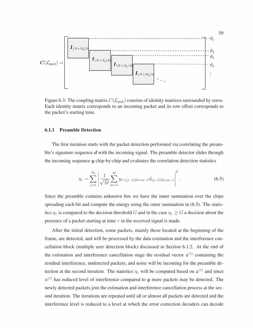
59
C(Lpack) =
θ1
θ2θ3
θ4...
I(N+Np)M
I(N+Np)M
I(N+Np)M
I(N+Np)M
I(N+NpNN )M
I(N+NpNN )M
I(N+NpNN )M
I(N+NpNN )M
Figure 6.3: The coupling matrix C(Lpack) consists of identity matrices surrounded by zeros.Each identity matrix corresponds to an incoming packet and its row offset corresponds tothe packet’s starting time.
6.1.1 Preamble Detection
The first iteration starts with the packet detection performed via correlating the pream-
ble’s signature sequence d with the incoming signal. The preamble detector slides through
the incoming sequence y chip-by-chip and evaluates the correlation detection statistics
ητ =
Np∑j=1
∣∣∣∣∣ 1√M
M∑m=1
yτ+(j−1)M+m−1d(j−1)M+m−1
∣∣∣∣∣2
. (6.5)
Since the preamble contains unknown bits we have the inner summation over the chips
spreading each bit and compute the energy using the outer summation in (6.5). The statis-
tics ητ is compared to the decision threshold G and in the case ητ ≥ G a decision about the
presence of a packet starting at time τ in the received signal is made.
After the initial detection, some packets, mainly those located at the beginning of the
frame, are detected, and will be processed by the data estimation and the interference can-
cellation block (multiple user detection block) discussed in Section 6.1.2. At the end of
the estimation and interference cancellation stage the residual vector z(1) containing the
residual interference, undetected packets, and noise will be incoming for the preamble de-
tection at the second iteration. The statistics ητ will be computed based on z(1) and since
z(1) has reduced level of interference compared to y more packets may be detected. The
newly detected packets join the estimation and interference cancellation process at the sec-
ond iteration. The iterations are repeated until all or almost all packets are detected and the
interference level is reduced to a level at which the error correction decoders can decode
60
the packets. A block diagram of the receiver is depicted in Fig. 6.4.
The thresholding parameter G may be determined assuming that the noise and interfer-
ence experienced by the packets in the multi-user environment can be approximated by a
Gaussian random variable. 3 In this case the statistics ητ follows a Chi-squared distribution
with Np degrees of freedom and non-centrality parameter Np(P +σ2I ) where σ2
I is the noise
and interference power and P is the power of the packet. If the packet is absent, ητ fol-
lows a central Chi-squared distribution with Np degrees of freedom. Supposing Np is large
enough, the Central Limit Theorem implies that ητ may be treated as a Gaussian random
variable with expectation and variance
Eητ = Np(P + σ2I ), var(ητ ) = Np(P + σ2
I )σ2I
for the case of a packet being present at time τ and
Eητ = Npσ2I , var(ητ ) = Npσ
4I
in the case it is absent. With this we may compute the probability of a false alarm as
pfa = Q
(G−Npσ
2I√
Npσ4I
),
where
Q(x) =1√2π
∫ ∞
x
exp(−t2/2)dt .
Fixing the false alarm probability to some value p0, and denoting q0 = Q−1(p0) allows us
to solve for the threshold
G = σ2I
√Np(√Np + q0) .
At iteration i the variance σ2I is estimated directly from the residual vector z(i−1) which
is processed for detection. To compute the decision threshold G for time τ the variance
σ2I needs to be computed for the part of the vector z(i−1) around the time index τ . The
length of this window may be chosen to be 3 − 5% of the packet length since σ2I varies
3This assumption relies on the Central Limit Theorem as we have a collection of a large number ofindependent interfering packets. The packets’ power distribution needs to satisfy Lindeberg Condition.
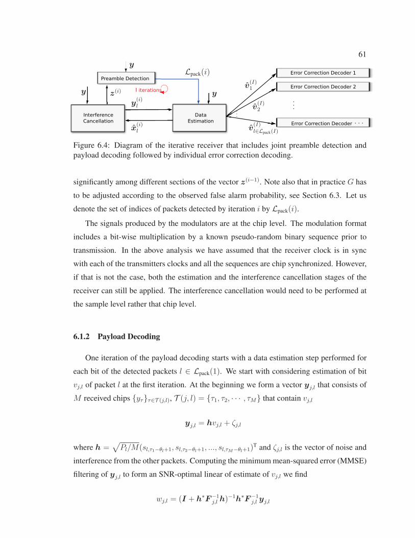
61y
Lpack(i)
y z(i)
y(i)l
x(i)l
yv(I)1
v(I)2
v(I)l∈Lpack(I)
. . .
. . .
I iterations
Interference Cancellation
DataEstimation
Preamble DetectionError Correction Decoder 1
Error Correction Decoder 2
Error Correction Decoder . . .
Figure 6.4: Diagram of the iterative receiver that includes joint preamble detection andpayload decoding followed by individual error correction decoding.
significantly among different sections of the vector z(i−1). Note also that in practice G has
to be adjusted according to the observed false alarm probability, see Section 6.3. Let us
denote the set of indices of packets detected by iteration i by Lpack(i).
The signals produced by the modulators are at the chip level. The modulation format
includes a bit-wise multiplication by a known pseudo-random binary sequence prior to
transmission. In the above analysis we have assumed that the receiver clock is in sync
with each of the transmitters clocks and all the sequences are chip synchronized. However,
if that is not the case, both the estimation and the interference cancellation stages of the
receiver can still be applied. The interference cancellation would need to be performed at
the sample level rather that chip level.
6.1.2 Payload Decoding
One iteration of the payload decoding starts with a data estimation step performed for
each bit of the detected packets l ∈ Lpack(1). We start with considering estimation of bit
vj,l of packet l at the first iteration. At the beginning we form a vector yj,l that consists of
M received chips {yτ}τ∈T (j,l), T (j, l) = {τ1, τ2, · · · , τM} that contain vj,l
yj,l = hvj,l + ζj,l
where h =√Pl/M(sl,τ1−θl+1, sl,τ2−θl+1, ..., sl,τM−θl+1)
T and ζj,l is the vector of noise and
interference from the other packets. Computing the minimum mean-squared error (MMSE)
filtering of yj,l to form an SNR-optimal linear of estimate of vj,l we find
wj,l = (I + h∗F−1j,l h)
−1h∗F−1j,l yj,l

62
where F j,l denotes the covariance matrix of ζj,l. One may compute the SNR of the signal
wj,l as
γj,l = h∗F−1j,l h.
In other words wj,l is a result of maximum ratio combining (MRC) of M received replicas
of vj,l. Since each bit vj,l can be 1 or −1, and takes each of the values with probability 1/2,
one can form a conditional expectation estimate vj,l of vj,l as
v(1)j,l = E(vj,l|wj,l) = tanh(wj,lγj,l).
The estimates v(1)j,l of the data bits may then be used instead of the true bits vj,l unknown to
the receiver to remodulate the packets. Since our estimation and interference cancellation
process is performing message passing on a graph for each bit vj,l we compute M estimates
v(1)j,l,m, m = 1, 2, · · · ,M . An estimate v
(1)j,l,m is obtained exactly as v(1)j,l discussed above but
without involving the observation yτm in the estimation process (i.e. we start with vector
yj,l,m where the yτm component is not present). We then produce a vector v(1)l by stacking
all the estimates v(1)j,l,m, re-modulate the packet and produce
x(1)l =
√Pl
Mdiag(d, sl)
(IMNp 0
0 P l
)[blR
TNp
v(1)l
]T.
At the next step we perform full interference cancellation to compute the residual vector of
noise and interference
z(1) = y −ALpack(1)x(1)Lpack(1)
which is forwarded to the preamble detector at the beginning of the second iteration. We
also compute vectors
y(1)l = y −ALpack(1)\lx
(1)Lpack(1)\l , l ∈ Lpack(1)
that will be used for estimation of data of packets l ∈ Lpack(1) at the second iteration. At the
beginning of the second iteration the packet detector produces an updated set of detected
packet indices Lpack(2). For the packets newly detected at the second iteration, i.e. l ∈
63
Lpack(2)\Lpack(1) the vector z(1) will be used for data estimation. The data estimation stage
of the second iteration computes x(2)l which is then passed to the interference canceller. The
entire process repeats for I iterations until all or almost all packets are detected and mutual
inter-packet interference is reduced to (approximately) the noise power level. After that the
packets are individually decoded by the error correction decoders. A detailed analysis of
convergence for such a system is given in [55] where it is proved that as preamble length
increases the system’s performance approaches the capacity of the channel.
6.2 AMP Algorithm for Joint Decoding and Detection
We notice that at each iteration we need to compute and store M copies of each esti-
mated packet bit and up to |Lpack(i)| different cancelled vectors. To reduce this computation
burden we will use the AMP framework [16][58]. At each iteration we compute only one
estimate for each data bit and each vector, and use correction factors to carefully approxi-
mate the original detection and decoding process.
The description of our proposed AMP algorithm based on series expansion and ap-
proximation of the passed messages is given in Fig. 6.5. The AMP version has a simple
description and saves orders of magnitude in complexity and storage for algorithm im-
plementation. Instead of storing the entire sparse matrix Ai matrix multiplications may be
done via explicit modulation as in Fig. 6.1. In practical conditions with no chip synchronic-
ity between the packets steps (6.6) and (6.7) can by done on sample basis.
6.3 Numerical Results
Fig. 6.6 demonstrates the simulated performance of the proposed random access system
with a joint detector and decoder. We consider a spreading factor M = 64, Np = 15 bit
preamble, N = 390 bit payload, and set the average rate of the new false alarms per
iteration to be < 10−5. Equal power distribution of the packets’ powers is considered 4
and the transmission is over the AWGN channel with signal-to-noise ratio (SNR) equal to
Pα/σ2. Binary error-correction codes optimal for the SNR observed at the output of the
4Unequal power distribution typically results in better iterative multi-user detector performances sincepower differences facilitate the convergence of the interference cancellation process. However, a modifiedsliding correlation detector needs to be considered in this case. For each time position detection at a numberof threshold levels needs to be attempted before sliding forward.
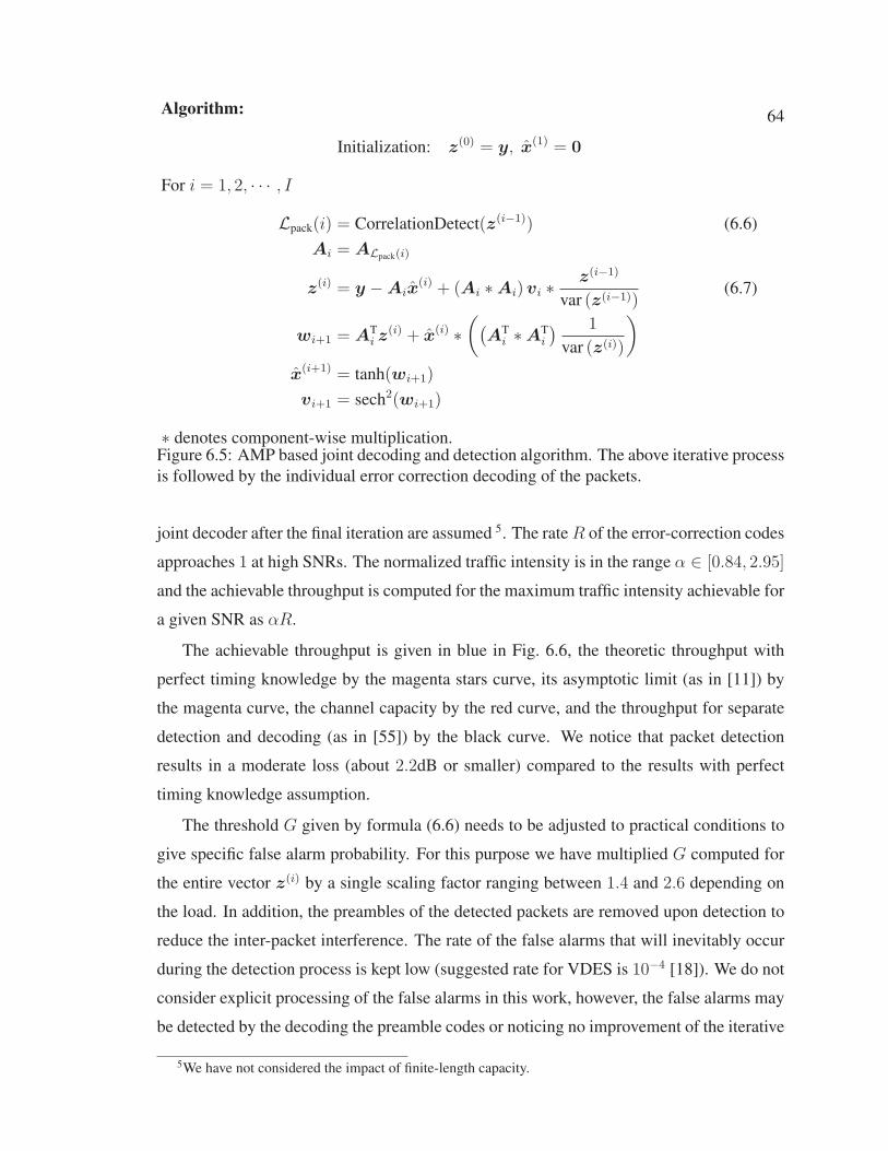
64Algorithm:
Initialization: z(0) = y, x(1) = 0
For i = 1, 2, · · · , I
Lpack(i) = CorrelationDetect(z(i−1)) (6.6)Ai = ALpack(i)
z(i) = y −Aix(i) + (Ai ∗Ai)vi ∗
z(i−1)
var (z(i−1))(6.7)
wi+1 = ATi z
(i) + x(i) ∗((
ATi ∗AT
i
) 1
var (z(i))
)x(i+1) = tanh(wi+1)
vi+1 = sech2(wi+1)
∗ denotes component-wise multiplication.Figure 6.5: AMP based joint decoding and detection algorithm. The above iterative processis followed by the individual error correction decoding of the packets.
joint decoder after the final iteration are assumed 5. The rate R of the error-correction codes
approaches 1 at high SNRs. The normalized traffic intensity is in the range α ∈ [0.84, 2.95]
and the achievable throughput is computed for the maximum traffic intensity achievable for
a given SNR as αR.
The achievable throughput is given in blue in Fig. 6.6, the theoretic throughput with
perfect timing knowledge by the magenta stars curve, its asymptotic limit (as in [11]) by
the magenta curve, the channel capacity by the red curve, and the throughput for separate
detection and decoding (as in [55]) by the black curve. We notice that packet detection
results in a moderate loss (about 2.2dB or smaller) compared to the results with perfect
timing knowledge assumption.
The threshold G given by formula (6.6) needs to be adjusted to practical conditions to
give specific false alarm probability. For this purpose we have multiplied G computed for
the entire vector z(i) by a single scaling factor ranging between 1.4 and 2.6 depending on
the load. In addition, the preambles of the detected packets are removed upon detection to
reduce the inter-packet interference. The rate of the false alarms that will inevitably occur
during the detection process is kept low (suggested rate for VDES is 10−4 [18]). We do not
consider explicit processing of the false alarms in this work, however, the false alarms may
be detected by the decoding the preamble codes or noticing no improvement of the iterative
5We have not considered the impact of finite-length capacity.

65
0 2 4 6 8 10 12 14 16 18 20 220
0.5
1
1.5
2
2.5
3
3.5
Tota
l Thr
ough
put [
bits
/s/H
z]
Signal-to-Noise ratio (overall) [dB]
Figure 6.6: The throughput achievable by the proposed random access system in bit/s/Hzas a function of the total system’s SNR.
data estimation of a non-existing packet.
Comparing the results with other random access techniques we notice that the achieved
traffic load of 2.95 of packets per packet length per spreading factor (bandwidth) is much
higher than 1 packets per slot or (packet length for unslotted systems) which is a typical
maximum for classic random access systems such as ALOHA [59], carrier-sense multiple
access (CSMA), self-organized TDMA used in AIS, contention resolution diversity slot-
ted ALOHA (CRDSA) [60], irregular resolution slotted ALOHA (IRSA) [61], coupled
random access [62], and even recently proposed systems such as coded slotted ALOHA
and enhanced contention resolution ALOHA (ECRA) [63] that can achieve loads up to 2
packets/packet length.

Chapter 7
Conclusions
In this thesis we have considered an implementation of the coupling information trans-
mission multi-user communication technique based on the spatial graph coupling princi-
ple [3]. We have proposed a demodulation technique based on approximate message pass-
ing (AMP) proposed by Donoho et al. [16] for compressed sensing problems. A version
of the AMP is derived for the multi-user situation to simplify the reception algorithm from
the perspective of implementation layout and computational complexity. At the same time
we make sure that operation in the “near-capacity” regime for a large number of multi-user
loads is preserved. The demodulation complexity per bit is constant per iteration and does
not scale with the processing gain, contrary to existing algorithms [2, 11, 12].
The algorithm, which is derived for the case of a theoretic scenario with perfectly orga-
nized message arrivals is the extended to a random-access case. An application of a satellite
uplink communication for maritime data exchange systems is considered and we demon-
strate that the achievable performance is superior that that of competing random access
mechanisms such as variations on ALOHA, ECRA, and uncoupled CDMA.
7.1 Future Work
It has been shown that coupling information transmission in conjunction with the de-
rived approximate message passing is an effective tool for communication over the AWGN
multiple access channel. There are several directions one could consider for future work:
� Unequal Power Case : While the equal power case is more difficult for inter-
symbol interference cancellation, in a realistic scenarion multiple user will always
have power differences. It is, for example, likely that users will transmit with differ-
ent power levels due to differing distances from the receiver. While, the algorithm in
its present form can accept unequal power messages it would be helpful to examine
the effectiveness of the AMP algorithm for the unequal power cases.
66

67
� Alternative Channels : We have considered the AWGN channel, however satel-
lite communication can be complicated by fading due to the ionosphere or tropo-
sphere, possible multi-path propagation, and changes of phase in the signal due to
the Doppler effect. It is worthwhile to consider how the AMP algorithm would be
modified to handle this situation, such as the inclusion of a bank of correlation de-
tectors and adjustment of the transmitter frequency based on approximate satellite
location broadcasted every frame via a bulletin board on the downlink channel.
Bibliography
[1] L. Pérez C. Schlegel. Trellis and turbo coding, 2nd edition. 2004.
[2] Dmitri Truhachev and Christian Schlegel. Coupling data transmission for capacity-achieving multiple-access communications. arXiv preprint arXiv:1209.5785, 2012.
[3] Christian Schlegel and Dmitry Truhachev. Multiple access demodulation in the liftedsignal graph with spatial coupling. Information Theory, IEEE Transactions on, 59(4):2459–2470, 2013.
[4] Alberto Jimenez Felström and Kamil Sh Zigangirov. Time-varying periodic con-volutional codes with low-density parity-check matrix. Information Theory, IEEETransactions on, 45(6):2181–2191, 1999.
[5] Michael Lentmaier, Arvind Sridharan, Daniel J Costello Jr, and Kamil Zigangirov.Iterative decoding threshold analysis for ldpc convolutional codes. IEEE Transactionson Information Theory, 56(10):5274–5289, 2010.
[6] Shrinivas Kudekar, Thomas J Richardson, and Rüdiger L Urbanke. Threshold satu-ration via spatial coupling: Why convolutional ldpc ensembles perform so well overthe bec. Information Theory, IEEE Transactions on, 57(2):803–834, 2011.
[7] Toshiyuki Tanaka. A statistical-mechanics approach to large-system analysis of cdmamultiuser detectors. Information Theory, IEEE Transactions on, 48(11):2888–2910,2002.
[8] Andrea Montanari and David Tse. Analysis of belief propagation for non-linear prob-lems: The example of cdma (or: How to prove tanaka’s formula). In InformationTheory Workshop, 2006. ITW’06 Punta del Este. IEEE, pages 160–164. IEEE, 2006.
[9] Christian Schlegel. Cdma with partitioned spreading. Communications Letters, IEEE,11(12):913–915, 2007.
[10] Dmitri Truhachev, Christian Schlegel, and Lukasz Krzymien. Low-complexity ca-pacity achieving two-stage demodulation/decoding for random matrix channels. InInformation Theory Workshop, 2007. ITW’07. IEEE, pages 584–589. IEEE, 2007.
[11] Dmitry Truhachev. Universal multiple access via spatially coupling data transmission.In Information Theory Proceedings (ISIT), 2013 IEEE International Symposium on,pages 1884–1888. IEEE, 2013.
[12] Keigo Takeuchi, Toshiyuki Tanaka, and Tsutomu Kawabata. Performance improve-ment of iterative multiuser detection for large sparsely spread cdma systems by spatialcoupling. Information Theory, IEEE Transactions on, 61(4):1768–1794, 2015.
68
69
[13] Christian Schlegel, Marat Burnashev, and Dmitri Truhachev. Generalized superpo-sition modulation and iterative demodulation: A capacity investigation. Journal ofElectrical and Computer Engineering, 2010:1, 2010.
[14] Li Ping, Lihai Liu, KY Wu, and Wai Kong Leung. On interleave-division multiple-access. In Communications, 2004 IEEE International Conference on, volume 5, pages2869–2873. IEEE, 2004.
[15] Peter Adam Hoeher and Tianbin Wo. Superposition modulation: myths and facts.Communications Magazine, IEEE, 49(12):110–116, 2011.
[16] David L Donoho, Arian Maleki, and Andrea Montanari. Message-passing algorithmsfor compressed sensing. Proceedings of the National Academy of Sciences, 106(45):18914–18919, 2009.
[17] Stefan Bober. Vdes - vhf data exchange system overview. In 2nd Workshop on VDES.
[18] Itu-r working party 5b .http://www.itu.int/en/ITU-R/study-groups/rsg5/rwp5b/Pages/default.aspx. Accessed:2016-03-30.
[19] IALA Recommendation for ITU-R M VDES.
[20] IEEE. Ieee standard, section 20.3.11.6 "802.11n-2009".http://standards.ieee.org/getieee802/download/802.11n-2009.pdf. Accessed:2016-05-24.
[21] Daniel J Costello and G David Forney. Channel coding: The road to channel capacity.Proceedings of the IEEE, 95(6):1150–1177, 2007.
[22] Shrinivas Kudekar, Tom Richardson, and Rudiger L Urbanke. Spatially coupled en-sembles universally achieve capacity under belief propagation. Information Theory,IEEE Transactions on, 59(12):7761–7813, 2013.
[23] Daniel J Costello, Lara Dolecek, Thomas Fuja, Joerg Kliewer, David Mitchell, andRoxana Smarandache. Spatially coupled sparse codes on graphs: Theory and practice.Communications Magazine, IEEE, 52(7):168–176, 2014.
[24] Keigo Takeuchi, Toshiyuki Tanaka, and Tsutomu Kawabata. A phenomenologicalstudy on threshold improvement via spatial coupling. IEICE Transactions on Fun-damentals of Electronics, Communications and Computer Sciences, 95(5):974–977,2012.
[25] Arvind Yedla, Yung-Yih Jian, Phong S Nguyen, and Henry D Pfister. A simple proofof threshold saturation for coupled scalar recursions. In Turbo Codes and IterativeInformation Processing (ISTC), 2012 7th International Symposium on, pages 51–55.IEEE, 2012.
70
[26] Arvind Yedla, Yung-Yih Jian, Phong S Nguyen, and Henry D Pfister. A simple proofof threshold saturation for coupled vector recursions. In Information Theory Work-shop (ITW), 2012 IEEE, pages 25–29. IEEE, 2012.
[27] Wassim M Haddad and VijaySekhar Chellaboina. Nonlinear dynamical systems andcontrol: a Lyapunov-based approach. Princeton University Press, 2008.
[28] Joel A Tropp. Just relax: Convex programming methods for identifying sparse signalsin noise. Information Theory, IEEE Transactions on, 52(3):1030–1051, 2006.
[29] David L Donoho, Michael Elad, and Vladimir N Temlyakov. Stable recovery ofsparse overcomplete representations in the presence of noise. Information Theory,IEEE Transactions on, 52(1):6–18, 2006.
[30] Emmanuel J Candes, Justin K Romberg, and Terence Tao. Stable signal recoveryfrom incomplete and inaccurate measurements. Communications on pure and appliedmathematics, 59(8):1207–1223, 2006.
[31] Emmanuel J Candes and Terence Tao. Decoding by linear programming. InformationTheory, IEEE Transactions on, 51(12):4203–4215, 2005.
[32] David L Donoho. Compressed sensing. Information Theory, IEEE Transactions on,52(4):1289–1306, 2006.
[33] Emmanuel Candes and Terence Tao. The dantzig selector: statistical estimation whenp is much larger than n. The Annals of Statistics, pages 2313–2351, 2007.
[34] Michael Elad and Michal Aharon. Image denoising via sparse and redundant rep-resentations over learned dictionaries. Image Processing, IEEE Transactions on, 15(12):3736–3745, 2006.
[35] Kostadin Dabov, Alessandro Foi, Vladimir Katkovnik, and Karen Egiazarian. Imagedenoising by sparse 3-d transform-domain collaborative filtering. Image Processing,IEEE Transactions on, 16(8):2080–2095, 2007.
[36] Kostadin Dabov, Alessandro Foi, Vladimir Katkovnik, and Karen Egiazarian. Im-age restoration by sparse 3d transform-domain collaborative filtering. In ElectronicImaging 2008, pages 681207–681207. International Society for Optics and Photonics,2008.
[37] Matan Protter and Michael Elad. Image sequence denoising via sparse and redundantrepresentations. Image Processing, IEEE Transactions on, 18(1):27–35, 2009.
[38] Michael Elad, J-L Starck, Philippe Querre, and David L Donoho. Simultaneous car-toon and texture image inpainting using morphological component analysis (mca).Applied and Computational Harmonic Analysis, 19(3):340–358, 2005.
[39] David L Donoho and Xiaoming Huo. Uncertainty principles and ideal atomic decom-position. Information Theory, IEEE Transactions on, 47(7):2845–2862, 2001.

71
[40] Yagyensh Chandra Pati, Ramin Rezaiifar, and PS Krishnaprasad. Orthogonal match-ing pursuit: Recursive function approximation with applications to wavelet decom-position. In Signals, Systems and Computers, 1993. 1993 Conference Record of TheTwenty-Seventh Asilomar Conference on, pages 40–44. IEEE, 1993.
[41] Shuchin Aeron, Venkatesh Saligrama, and Manqi Zhao. Information theoretic boundsfor compressed sensing. Information Theory, IEEE Transactions on, 56(10):5111–5130, 2010.
[42] Galen Reeves and Michael Gastpar. Compressed sensing phase transitions: Rigorousbounds versus replica predictions. In Information Sciences and Systems (CISS), 201246th Annual Conference on, pages 1–6. IEEE, 2012.
[43] Yihong Wu and Sergio Verdú. Rényi information dimension: Fundamental limits ofalmost lossless analog compression. Information Theory, IEEE Transactions on, 56(8):3721–3748, 2010.
[44] Yihong Wu and Sergio Verdú. Optimal phase transitions in compressed sensing. In-formation Theory, IEEE Transactions on, 58(10):6241–6263, 2012.
[45] Dongning Guo, Dror Baron, and Shlomo Shamai. A single-letter characterizationof optimal noisy compressed sensing. In Communication, Control, and Computing,2009. Allerton 2009. 47th Annual Allerton Conference on, pages 52–59. IEEE, 2009.
[46] David L Donoho, Adel Javanmard, and Alessandro Montanari. Information-theoretically optimal compressed sensing via spatial coupling and approximate mes-sage passing. Information Theory, IEEE Transactions on, 59(11):7434–7464, 2013.
[47] Shrinivas Kudekar and Henry D Pfister. The effect of spatial coupling on compressivesensing. In Communication, Control, and Computing (Allerton), 2010 48th AnnualAllerton Conference on, pages 347–353. IEEE, 2010.
[48] Florent Krzakala, Marc Mézard, François Sausset, YF Sun, and Lenka Zdeborová.Statistical-physics-based reconstruction in compressed sensing. Physical Review X, 2(2):021005, 2012.
[49] Yonina C Eldar and Gitta Kutyniok. Compressed sensing: theory and applications.Cambridge University Press, 2012.
[50] Upamanyu Madhow and Michael B Pursley. Acquisition in direct-sequence spread-spectrum communication networks: an asymptotic analysis. Information Theory,IEEE Transactions on, 39(3):903–912, 1993.
[51] Giovanni E Corazza and Vittorio Degli-Esposti. Acquisition-based capacity estimatesfor cdma with imperfect power control. In Spread Spectrum Techniques and Applica-tions, 1994. IEEE ISSSTA’94., IEEE Third International Symposium on, pages 325–329. IEEE, 1994.

72
[52] Mark C Reed, Leif W Hanlen, and Giovanni E Corazza. Return-link code acquisi-tion for 1-d and 2-d with ds-cdma for high-capacity multiuser systems. VehicularTechnology, IEEE Transactions on, 57(1):324–334, 2008.
[53] Bathiya Senanayake, Mark C Reed, and Zhenning Shi. Timing acquisition for multi-user idma. In Communications, 2008. ICC’08. IEEE International Conference on,pages 5077–5081. IEEE, 2008.
[54] Dmitri Truhachev. Asymptotic analysis of joint timing acquisition and multiple packetreception. In Wireless Communications and Networking Conference (WCNC), 2011IEEE, pages 1869–1874. IEEE, 2011.
[55] Dmitry Truhachev. Packet acquisition for spatially coupling information transmission.In Communications Workshops (ICC), 2014 IEEE International Conference on, pages495–500. IEEE, 2014.
[56] Dmitri Truhachev. Achieving awgn multiple access channel capacity with spatialgraph coupling. Communications Letters, IEEE, 16(5):585–588, 2012.
[57] Burkhard Militzer, Michele Zamparelli, and Dieter Beule. Evolutionary search forlow autocorrelated binary sequences. IEEE Transactions on Evolutionary Computa-tion, 2(1):34–39, 1998.
[58] Alfred M Bruckstein, David L Donoho, and Michael Elad. From sparse solutions ofsystems of equations to sparse modeling of signals and images. SIAM review, 51(1):34–81, 2009.
[59] Norman Abramson. The aloha system: another alternative for computer communica-tions. In Proceedings of the November 17-19, 1970, fall joint computer conference,pages 281–285. ACM, 1970.
[60] Enrico Casini, Riccardo De Gaudenzi, and Od R Herrero. Contention resolutiondiversity slotted aloha (crdsa): An enhanced random access schemefor satellite accesspacket networks. Wireless Communications, IEEE Transactions on, 6(4):1408–1419,2007.
[61] Gianluigi Liva. Graph-based analysis and optimization of contention resolution di-versity slotted aloha. Communications, IEEE Transactions on, 59(2):477–487, 2011.
[62] Gianluigi Liva, Enrico Paolini, Michael Lentmaier, and Marco Chiani. Spatially-coupled random access on graphs. In Information Theory Proceedings (ISIT), 2012IEEE International Symposium on, pages 478–482. IEEE, 2012.
[63] Federico Clazzer and Christian Kissling. Enhanced contention resolution aloha-ecra.In Systems, Communication and Coding (SCC), Proceedings of 2013 9th Interna-tional ITG Conference on, pages 1–6. VDE, 2013.
Related Documents