Coupled Oscillations

187

Chapter 10. Coupled Oscillations (Most of the material presented in this chapter is taken from Thornton and Marion, Chap. 12.)

In Chapter 2, we studied systems that exhibit oscillations in their response, either naturally or when driven by an external force. We now generalized the problem to include situations where not only multiple oscillation modes or frequencies are possible, but also when there are interactions amongst the different oscillating components of a given system. This leads us to the study of the more complicated topic of coupled oscillations.

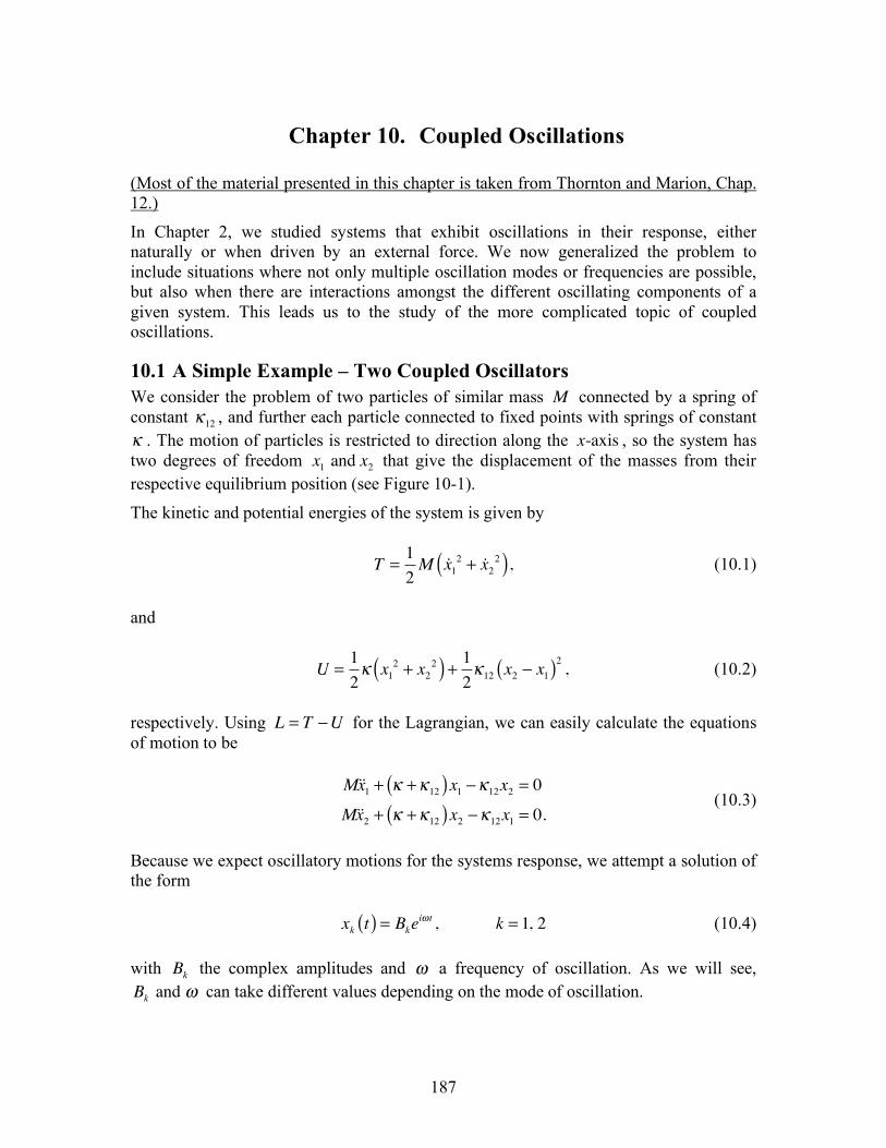
10.1 A Simple Example – Two Coupled Oscillators We consider the problem of two particles of similar mass M connected by a spring of constant !

12, and further each particle connected to fixed points with springs of constant

! . The motion of particles is restricted to direction along the x-axis , so the system has two degrees of freedom x

1 and x

2 that give the displacement of the masses from their

respective equilibrium position (see Figure 10-1).

The kinetic and potential energies of the system is given by

T =1

2M !x

1

2+ !x

2

2( ), (10.1)

and

U =1

2! x

1

2+ x

2

2( ) +1

2!12x2" x

1( )2

, (10.2)

respectively. Using L = T !U for the Lagrangian, we can easily calculate the equations of motion to be

M!!x1+ ! +!

12( )x1 "!12x2 = 0

M!!x2+ ! +!

12( )x2 "!12x1 = 0. (10.3)

Because we expect oscillatory motions for the systems response, we attempt a solution of the form x

kt( ) = B

kei! t, k = 1, 2 (10.4)

with B

k the complex amplitudes and ! a frequency of oscillation. As we will see,

Bk and ! can take different values depending on the mode of oscillation.

188

Figure 10-1 – Two masses connected by a spring to each other and by other springs to fixed points.

Using equations (10.4) along with !!xk= !"

2xk, we can transform equations (10.3) to

!M"

2B1ei" t

+ # +#12( )B1e

i" t!#

12B2ei" t

= 0

!M"2B2ei" t

+ # +#12( )B2e

i" t!#

12B1ei" t

= 0. (10.5)

Regrouping terms and simplifying (by dropping the common exponential term), this equation can be written in a matrix form as

! +!

12"# 2

M( ) "!12

"!12

! +!12"# 2

M( )

$

%&&

'

())

B1

B2

*+,

-./= 0. (10.6)

As usual, for this system of equations to have a non-trivial solution the determinant of the matrix on the left side of equation (10.6) must vanish. That is,

! +!

12"#

2M( ) "!

12

"!12

! +!12"#

2M( )

= 0. (10.7)

The expansion of this determinant yields the so-called characteristic equation of the system ! +!

12"#

2M( )

2

"!12

2= 0, (10.8)

or, if we take the square root, ! +!

12"#

2M = ±!

12. (10.9)

Solving for ! , we find the characteristic frequencies (or eigenfrequencies, or eigenvalues) of the system. In this case, there are four frequencies: ±!

1 and ±!

2, with

189

!1=

" + 2"12

M, !

2=

"

M. (10.10)

If we set ! = ±!

1 in equations (10.4) and insert it in equation (10.6), we find that

B1= !B

2. Similarly, if we set ! = ±!

2 in equations (10.4) and insert it in equation

(10.6), we find that B1= B

2. If we associate one amplitude constant for each

eigenfrequency, i.e., Bi

± for ±!

i, we can write the complete solution to the system of

equations (10.6) as

x1t( ) = B

1

+ei!1t + B

1

"e" i!1t + B

2

+ei!2 t + B

2

"e" i!2 t

x2t( ) = "B

1

+ei!1t " B

1

"e" i!1t + B

2

+ei!2 t + B

2

"e" i!2 t .

(10.11)

We see from this last set of equations that the position of the particles are both functions of the two frequencies !

1 and !

2, The two degrees of freedom x

1t( ) and x

2t( ) are not,

therefore, independent of each other. We would like to find out if there exists a transformation that will lead to a new set of coordinates that would be decoupled along the different modes of oscillation. Inspection of equations (10.11) suggests an obvious candidate. That is, if we introduce the following new coordinates

!1= x

1" x

2

!2= x

1+ x

2, (10.12)

or,

x1=1

2!1+!

2( )

x2=1

2!2"!

1( ), (10.13)

and we substitute this last set of equations into equations (10.5) we find

M !!!1+ !!!

2( ) + " + 2"12( )!1 +"!2 = 0

M !!!1# !!!

2( ) + " + 2"12( )!1 #"!2 = 0.

(10.14)

By adding and subtracting the last two equations, we easily solve this system to obtain

M !!!1+ " + 2"

12( )!1 = 0

M !!!2+"!

2= 0.

(10.15)

We can proceed as was done for x

1t( ) and x

2t( ) to find that

190

!1t( ) = C1

+ei"1t + C

1

#e# i"1t

!2t( ) = C2

+ei"2 t + C

2

#e# i"2 t ,

(10.16)

where the frequencies !

1 and !

2 are as defined by equations (10.10). We see from

equations (10.15) and (10.16) that !1t( ) and !

2t( ) are decoupled and independent.

The constants Ci

± are to be determined from the initial conditions. For example, if we have x

10( ) = !x

20( ) and

!x10( ) = ! !x

20( ) , then

!20( ) = !!

20( ) = 0 and C

2

+= C

2

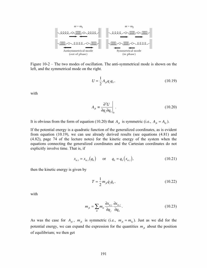
!= 0 ;

that is, !2t( ) = 0 at all times. We find that in this case the particles oscillate out of phase

with each other at frequency !1; this is the anti-symmetrical mode of oscillation.

Conversely, if we set x10( ) = x

20( ) and

!x10( ) = !x

20( ) , we find that !

1t( ) = 0 at all

times. The particles then oscillate in phase with each other at frequency !2; this is the

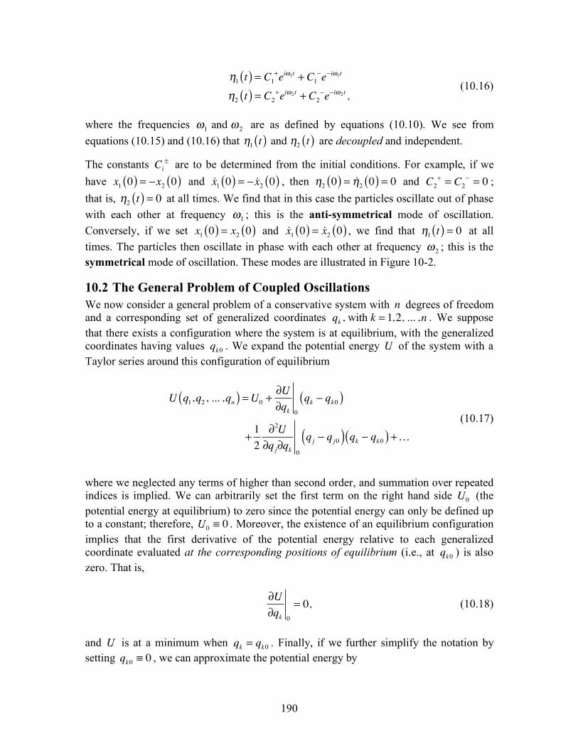
symmetrical mode of oscillation. These modes are illustrated in Figure 10-2.

10.2 The General Problem of Coupled Oscillations We now consider a general problem of a conservative system with n degrees of freedom and a corresponding set of generalized coordinates qk , with k = 1,2, ... ,n . We suppose that there exists a configuration where the system is at equilibrium, with the generalized coordinates having values qk0 . We expand the potential energy U of the system with a Taylor series around this configuration of equilibrium

U q1,q

2, ... ,qn( ) =U0

+!U

!qk 0

qk " qk0( )

+1

2

!2U

!qj!qk0

qj " qj0( ) qk " qk0( ) +…

(10.17)

where we neglected any terms of higher than second order, and summation over repeated indices is implied. We can arbitrarily set the first term on the right hand side U

0 (the

potential energy at equilibrium) to zero since the potential energy can only be defined up to a constant; therefore, U

0! 0 . Moreover, the existence of an equilibrium configuration

implies that the first derivative of the potential energy relative to each generalized coordinate evaluated at the corresponding positions of equilibrium (i.e., at qk0 ) is also zero. That is,

!U

!qk 0

= 0, (10.18)

and U is at a minimum when qk = qk0 . Finally, if we further simplify the notation by setting qk0 ! 0 , we can approximate the potential energy by

191

Figure 10-2 – The two modes of oscillation. The anti-symmetrical mode is shown on the left, and the symmetrical mode on the right.

U =1

2Ajkqjqk , (10.19)

with

Ajk !"2U

"qj"qk0

. (10.20)

It is obvious from the form of equation (10.20) that Ajk is symmetric (i.e., Ajk = Akj ).

If the potential energy is a quadratic function of the generalized coordinates, as is evident from equation (10.19), we can use already derived results (see equations (4.81) and (4.82), page 74 of the lecture notes) for the kinetic energy of the system when the equations connecting the generalized coordinates and the Cartesian coordinates do not explicitly involve time. That is, if x

! ,i = x! ,i qk( ) or qk = qk x! ,i( ), (10.21)

then the kinetic energy is given by

T =1

2mjk!qj !qk , (10.22)

with

mjk = m!

"x! ,i

"qj!

#"x! ,i

"qk. (10.23)

As was the case for Ajk , mjk is symmetric (i.e., mjk = mkj ). Just as we did for the potential energy, we can expand the expression for the quantities mjk about the position of equilibrium; we then get

192

mjk q1,… ,qn( ) = mjk ql0( ) +!mjk

!ql 0

ql +… (10.24)

However, in order to be consistent in the accuracy kept for both the potential and kinetic energies, we only keep the first term on the right hand side of equation (10.24). This way, both expressions are valid to the second order (in velocities for the kinetic energy, and in displacement for the potential energy). We then write

T =1

2mjk!qj !qk

U =1

2Ajkqjqk

(10.25)

with the understanding that mjk consists only of the first term in the expansion on the right side of equation (10.24).

We are now interested in solving for the equations of motion of the system, using the Lagrangian formalism. That is,

!L!qk

"d

dt

!L! !qk

#

$%&

'(= 0, (10.26)

which, in this case simplifies to

!U!qk

+d

dt

!T! !qk

"

#$%

&'= 0. (10.27)

Using equations (10.25), the equations of motion are reduced to the following

Ajkqj + mjk!!qj = 0 (10.28)

Equations (10.28) represent a set of coupled second-order differential equations with constant coefficients. Since we expect oscillatory motions, we propose a solution of the form qj t( ) = aje

i ! t"#( ), (10.29)

where the amplitudes aj are real. Inserting this equation in equations (10.28), we find for the equations of motion Ajk !"

2mjk( )aj = 0 (10.30)

193

Alternatively, the system of equations (10.30) can be written in a matrix form A !"

2m( ) #a = 0, (10.31)

where the matrices A and m are composed of the elements Ajk and mjk , respectively (remember that A and m are symmetric). In order to get a non-trivial solution to this equation, the determinant of the quantity in parentheses must vanish A !"

2m = 0. (10.32)

This determinant is called the characteristic or secular equation and is an equation of degree n in ! 2 . The corresponding n roots !

r

2 are the characteristic frequencies or eigenfrequencies of the system. The eigenvector associated with a given root !

r can be

evaluated by inserting it back in equations (10.30) to determine the ratios a1:a

2: ... :a

n

(this is similar to what we did in Chapter 9 when determining the principle axes of the inertia tensor). If we represent by ajr the jth component of the rth eigenvector, we can write the generalized coordinate qj as a linear combination of the solutions for each root qj t( ) = ajre

i !r t"#r( )

r

$ . (10.33)

It is, however, understood that the actual solution must be real (in a mathematical sense) and we must, therefore, take real part of equation (10.33). That is, q

jt( ) = a

jrcos !

rt " #

r( )r

$ . (10.34)

Example We apply the formalism just developed to the previous problem of the two masses connected by springs to find the characteristics frequencies. Solution. We know from equation (10.2) that

U =1

2! x

1

2+ x

2

2( ) +1

2!12x2" x

1( )2

. (10.35)

The elements of the matrix A are therefore (from equation (10.20))

194

A11=!2U

!x1

2

0

=" +"12

A12= A

21=

!2U

!x1!x

2 0

= #"12

A22=!2U

!x2

2

0

=" +"12.

(10.36)

The kinetic energy of the system is

T =1

2M !x

1

2+ !x

2

2( ), (10.37)

and the elements of the matrix m are, from equation (10.23),

m11= m

22= M

m12= m

21= 0.

(10.38)

The determinant is then given by

! +!

12"#

2M( ) "!

12

"!12

! +!12"#

2M( )

= 0, (10.39)

which is the same equation (10.7) that we obtained before. The eigenfrequencies are therefore unchanged at

!1=

" + 2"12

M, !

2=

"

M. (10.40)

10.3 Orthogonality of the Eigenvectors and the Normal Coordinates According to equation (10.30), we can write for the sth root !

s

! s

2mjkaks = Ajkaks , (10.41)

and a similar one for the another root, say !

r

! r

2mjkajr = Ajkajr , (10.42)

where we used the symmetry of the m and A matrices. We now multiply equation (10.41) by ajr and the equation (10.42) by a

ks, and subtract the two. We then find that

195

! r

2"! s

2( )ajrmjkaks = 0. (10.43) If r ! s and !

r

2" !

s

2 , then we must have that ajrmjkaks = 0, r ! s. (10.44) If r = s (and, therefore, !

r

2"!

s

2= 0 ) then, the double product ajrmjkaks may not

vanish. This can, in fact, be verified by calculating the kinetic energy using equation (10.34)

T =1

2mjk!qj !qk

=1

2mjk ! rajr sin ! rt " #r( )

r

$%

&'

(

)* ! saks sin ! st " # s( )

s

$%

&'

(

)*

=1

2! r! s

r ,s

$ sin ! rt " #r( )sin ! st " # s( ) ajrmjkaks%& ().

(10.45)

But inserting equation (10.44) when r = s and !

r

2=!

s

2 , equation (10.45) reduces to

T =1

2! r

2sin

2 ! rt " #r( )r

$ ajrmjkakr%& '(, (10.46)

and since both T and !

r

2sin

2!

rt " #

r( ) are greater than zero, it must be that ajrmjkakr > 0. (10.47) Moreover, because we can only measure the ratios of the components ajr , we arbitrarily normalize them according to ajrmjkakr = 1. (10.48) On the other hand, if we have a case of degeneracy for one eigenvalue !

r

2 (i.e., r ! s but !

r

2=!

s

2 ), we cannot outright say that equation (10.44) is satisfied (since !

r

2"!

s

2= 0 in equation (10.43)). However, it turns out that we can always ensure that

this is so (i.e., that ajrmjkaks = 0 ). For example, if we assume that two different vectors

ar and a

s share the same eigenfrequency ! 2 , then we can also say from equation (10.31)

that

196

A !ai="

2m !a

i, (10.49)

with i = r, s . These two vectors bring six unknowns (one per component), for which we can match two equations of motions (i.e., from equation (10.49)), one equation to ensure the sought after orthogonality of the vectors (i.e., ajrmjkaks = 0 ), and two equations to normalize the vectors (i.e., ajrmjkakr = 1 , and a similar equation for s ). This gives us five equations for six unknowns. The fact that we have fewer equations than unknowns ensures non-trivial solutions (we can, for example, arbitrarily set the value of one of the unknowns and solve for the remaining five unknowns using the five aforementioned equations). Thus, we can show that the orthgonality between eigenvectors is respected even in the case of degeneracy in the values of the eigenfrequencies.

We can, therefore, combine equations (10.44) and (10.48) to get, for any r and s , the following relation ajrmjkaks = !rs (10.50)

We say that the eigenvectors are orthonornal, in the sense defined in this last equation. It is customary to refer to the frequencies !

r as being the different modes of oscillation

of the system. The vectors ar are the corresponding eigenvectors associated with these

modes. It is important to note that we have now imposed a normalization constraint on the eignvectors that was not assumed when we initially solved the problem with equation (10.29) for the generalized coordinates qj t( ) . We must therefore introduce a new set of quantities !

r that are to be multiplied to the vectors a

r. More precisely, we now have

qj t( ) = ! rajre

i "r t#$r( )

r

% , (10.51)

which we promptly simplify by introducing yet another constant (but, this time complex) !r= "

rei#r such that

qj t( ) = !rajre

i"r t

r

# . (10.52)

We further define the so-called normal coordinates !

r as

!

rt( ) " #

rei$

rt (10.53)

so that q

jt( ) = a

jr!rt( )

r

" (10.54)

197

Finally, it fairly straightforward to show, using the orthonormality condition of equation (10.50), that the form of the kinetic and potential energies are significantly simplified by the use of the normal coordinates. A few lines of calculations reveal that

T =1

2!!r

2

r

"

U =1

2#

r

2!r

2

r

" .

(10.55)

Applying the Lagrange equations to these two equations we get

!!!r+"

r

2!r= 0. (10.56)

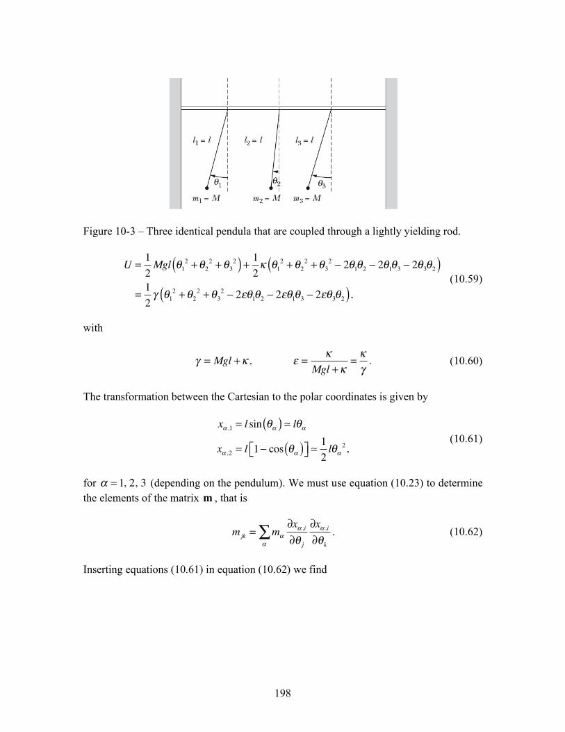
We have the interesting result that this new system of second-order differential equations is completely decoupled, i.e. we have n independent equations of motions. Example Three linearly coupled plane pendula. Three identical pendula of mass M and length l are suspended from a slightly yielding rod, which brings a certain amount of coupling ! between each pair of pendula (see Figure 10-3). Find the eigenfrequencies, eigenvectors, and the normal modes of oscillation. Consider only the case of small oscillations. Solution. We start by evaluating the kinetic and potential energies; we have

T =1

2Ml

2 !!1

2+ !!

2

2+ !!

3

2( )

U = Mgl 1" cos !1( )#$ %& + 1" cos !

2( )#$ %& + 1" cos !3( )#$ %&{ }

+1

2' !

1"!

2( )2

+ !1"!

3( )2

+ !3"!

2( )2#

$%&.

(10.57)

In the case of a small oscillation, we have

1! cos "( ) ! 1! 1!1

2" 2#

$%&'(=1

2" 2 , (10.58)

so we can re-write the potential energy as

198

Figure 10-3 – Three identical pendula that are coupled through a lightly yielding rod.

U =

1

2Mgl !

1

2+!

2

2+!

3

2( ) +1

2" !

1

2+!

2

2+!

3

2 # 2!1!2# 2!

1!3# 2!

3!2( )

=1

2$ !

1

2+!

2

2+!

3

2 # 2%!1!2# 2%!

1!3# 2%!

3!2( ),

(10.59)

with

! = Mgl +" , # ="

Mgl +"="

!. (10.60)

The transformation between the Cartesian to the polar coordinates is given by

x! ,1 = l sin "!( ) ! l"!

x! ,2 = l 1# cos "!( )$% &' !1

2l"!

2, (10.61)

for ! = 1, 2, 3 (depending on the pendulum). We must use equation (10.23) to determine the elements of the matrix m , that is

mjk = m!

"x! ,i

"# j!

$"x! ,i

"#k

. (10.62)

Inserting equations (10.61) in equation (10.62) we find

199

m11= Ml

21+ !!

1

2( )

m22= Ml

21+ !!

2

2( )

m33= Ml

21+ !!

3

2( )m12= m

13= m

23= 0.

(10.63)

However, we must remember from the discussion following equation (10.24) that since we want to keep the precision of the potential energy to the second-order in the generalized coordinates, we must only keep the lowest order terms in equations (10.63). We therefore make the following approximation m

11= m

22= m

33= Ml

2, (10.64)

and

m = Ml2

1 0 0

0 1 0

0 0 1

!

"

###

$

%

&&&

. (10.65)

Using equation (10.20) we can directly evaluate the matrix A from equation (10.59) for the potential energy

A = !

1 "# "#

"# 1 "#

"# "# 1

$

%

&&&

'

(

)))

. (10.66)

We must now evaluate the following determinant to determine the eigenfrequencies

A !" 2m =

# !" 2Ml

2!#$ !#$

!#$ # !" 2Ml

2!#$

!#$ !#$ # !" 2Ml

2

= 0. (10.67)

Expanding this determinant, we have ! "# 2

Ml2( )3

" 2! 3$ 3 " 3! 2$ 2 ! "# 2Ml

2( ) = 0, (10.68) which can be factored into ! 2

Ml2" # " #$( )

2

! 2Ml

2" # + 2#$( ) = 0. (10.69)

The roots are therefore

200

!1

2=!

2

2=" 1+ #( )

Ml2

=Mgl + 2$

Ml2

!3

2=" 1% 2#( )

Ml2

=Mgl %$

Ml2.

(10.70)

We notice from the first of equations (10.70) that the system is degenerate, since !1

2=!

2

2 .

Having evaluated the eigenfrequencies, we can insert them back into the equations of motion to find the eigenvectors a

r. That is, starting with !

3

2 ,

Ajk !" 3

2mjk( )aj3 = 0, (10.71)

or

2!"a

13# !"a

23# !"a

33= 0

#!"a13+ 2!"a

23# !"a

33= 0.

(10.72)

We only used two of the three equations of motion since we only have two unknowns (i.e., two ratios taken from the components of a

3). The third equation of motion will

automatically be satisfied. From equations (10.72) we find

a13= a

23= a

33=1

3, (10.73)

where the vector was normalized.

For the degenerate case, we insert !1

2(=!

2

2) in the equations of motion to calculate

a1 and a

2. This yields

!"# a

11+ a

21+ a

31( ) = 0

!"# a12+ a

22+ a

32( ) = 0. (10.74)

The orthogonality condition aj1mjkak2 = 0 , and the normalization conditions (imposed on the eigenvectors) respectively give

Ml2a11a12+ a

21a22+ a

31a32( ) = 0

a11

2+ a

21

2+ a

31

2= 1

a12

2+ a

22

2+ a

32

2= 1.

(10.75)

201

We therefore have five equations for six unknowns, which guaranties non-trivial solutions. If we arbitrarily set a

11= 0 , we have from the first of equations (10.74) and the

second of equations (10.75) that

a21= !a

31=1

2. (10.76)

Then, from the first of equations (10.75) and the second of equations (10.74)

a22= a

32= !

1

2a12, (10.77)

and, finally, from the last of equations (10.75)

a12=

2

3. (10.78)

The three eigenvectors can be written as

a1=1

20, 1, !1( )

a2=1

62, !1, !1( )

a3=1

31, 1, 1( ).

(10.79)

We see that the third normal mode corresponds to an in-phase oscillation with the three pendula moving in the same direction with the same amplitude. On the other hand, the first two normal modes have an out-of-phase character. In the first mode the second and third pendula are moving in opposite directions with equal amplitude, while in the second mode the first pendulum is moving in opposite direction of the other two, and at twice their amplitude.