Coupled multi-physics simulations of the Molten Salt …samofar.eu/wp-content/uploads/2016/11/MScThesis-eirikEidePettersen.… · thermal-hydraulics and spatial neutronics Master

Coupled multi-physics simulations of theMolten Salt Fast Reactor using coarse-meshthermal-hydraulics and spatial neutronics

Master thesis by

Eirik Eide Pettersen

Supervised by:Konstantin Mikityuk

@

Paul Scherrer InstitutVilligen, Switzerland

Universite Paris-SaclaySeptember 2016

Abstract

The Molten Salt Fast Reactor (MSFR) perfectly embodies the tantalising prospects ofnext-generation nuclear power reactors by offering considerable improvements in areas of

sustainability, safety, and economics, while avoiding greenhouse gas emissions. However, muchresearch is needed to mature the conceptual design, not least in the field of computational

physics. As with all liquid-fuelled molten salt reactors (MSRs), the MSFR is characterised by aparticularly strong coupling between neutronics and thermal-hydraulics induced by combining the

fuel and coolant into the same liquid. Investigations into the dynamic behaviour of MSRs thusrequire the use of coupled multi-physics codes. A number of such tools have emerged in recent

years, most based on computational fluid dynamics (CFD).

In this thesis work, an alternative approach is taken with the use of a coupled tool consisting ofthe coarse-mesh, thermal-hydraulics system code TRACE and the three-dimensional neutron

diffusion solver PARCS. This tool offers a number of advantages compared to CFD-basedapproaches, such as low computational requirements, established numerical solution and coupling

methodologies, native two-phase fluid capabilities, and simplicity in modelling complex plantcomponents across primary, intermediate, and turbine circuits. Conversely, the coarse-mesh andsimplified equations solution strategy employed by TRACE-PARCS requires compromising theaccuracy of the calculations, and suffers from limitations in problem geometry modelling. Theoverarching goal of this work is to assess the ability of the coupled TRACE-PARCS code to

accurately compute dynamic behaviour of the MSFR. In doing so, many characteristicphenomena of molten salt reactors have been investigated. A secondary aim is to illustrate and

explain these distinguishing and unconventional features.

Presented simulations of the MSFR have been performed in a simplified, axially-symmetricbenchmark model implemented separately in both TRACE and PARCS, as well as in the MonteCarlo code Serpent which is used for cross section generation. Neutronic and thermal-hydraulic

steady-state behaviour has been characterised and compared with alternative solvers. Following acalibration procedure, satisfactory agreement is found between steady-state solutions produced byTRACE and a higher-accuracy solver based on CFD. Similarly, the neutronic solution calculatedby PARCS correlates well with Serpent after calibrating the boundary conditions. The coupled

TRACE-PARCS code generally reproduces the dynamic behaviour of the MSFR as predicted byother multi-physics tools. Considerable discrepancies are present, but most are explained by

differences in modelling choices, and those that remain are likely caused by dissimilarities in theunderlying methods. Although TRACE-PARCS simulations could be run on a single processor,computational times were prohibitively long. Clear potentials for accelerating the computational

procedure have been identified.

The presented work paves the way for further investigation of the MSFR, and allows forstraightforward extension to full plant modelling and asymmetric transient investigation.Composite codes employing a CFD solver for core calculations coupled with TRACE for

out-of-core components represent another promising direction in which to progress.

Contents

1 Introduction 5

1.1 Background and motivation . . . . . . . . . . . . . . . . . . . . . . . . . . . . . . . . 5

1.2 Objectives and outline . . . . . . . . . . . . . . . . . . . . . . . . . . . . . . . . . . . 7

2 Molten salt reactors 8

2.1 History . . . . . . . . . . . . . . . . . . . . . . . . . . . . . . . . . . . . . . . . . . . 8

2.2 Features . . . . . . . . . . . . . . . . . . . . . . . . . . . . . . . . . . . . . . . . . . . 9

2.3 The Molten Salt Fast Reactor . . . . . . . . . . . . . . . . . . . . . . . . . . . . . . . 10

2.3.1 Salts specification . . . . . . . . . . . . . . . . . . . . . . . . . . . . . . . . . 12

2.3.2 Benchmark specification . . . . . . . . . . . . . . . . . . . . . . . . . . . . . . 13

3 Computational tools 15

3.1 TRACE . . . . . . . . . . . . . . . . . . . . . . . . . . . . . . . . . . . . . . . . . . . 15

3.1.1 Principal equations . . . . . . . . . . . . . . . . . . . . . . . . . . . . . . . . . 15

3.1.2 Primary circuit model . . . . . . . . . . . . . . . . . . . . . . . . . . . . . . . 17

3.1.3 Heat exchanger and pump models . . . . . . . . . . . . . . . . . . . . . . . . 18

3.2 Serpent . . . . . . . . . . . . . . . . . . . . . . . . . . . . . . . . . . . . . . . . . . . 19

3.3 PARCS . . . . . . . . . . . . . . . . . . . . . . . . . . . . . . . . . . . . . . . . . . . 20

3.4 Coupling methodology . . . . . . . . . . . . . . . . . . . . . . . . . . . . . . . . . . . 21

4 Results 23

4.1 Steady-state behaviour . . . . . . . . . . . . . . . . . . . . . . . . . . . . . . . . . . . 23

4.1.1 Neutronics . . . . . . . . . . . . . . . . . . . . . . . . . . . . . . . . . . . . . 24

4.1.2 Blanket behaviour . . . . . . . . . . . . . . . . . . . . . . . . . . . . . . . . . 27

4.1.3 Thermal-hydraulics . . . . . . . . . . . . . . . . . . . . . . . . . . . . . . . . . 28

4.2 Transient behaviour . . . . . . . . . . . . . . . . . . . . . . . . . . . . . . . . . . . . 34

4.2.1 Unprotected loss of heat sink . . . . . . . . . . . . . . . . . . . . . . . . . . . 35

4.2.2 Unprotected pump over-speed . . . . . . . . . . . . . . . . . . . . . . . . . . . 37

4.2.3 Unprotected over-cooling . . . . . . . . . . . . . . . . . . . . . . . . . . . . . 38

4.2.4 Unprotected loss of flow . . . . . . . . . . . . . . . . . . . . . . . . . . . . . . 40

5 Conclusions and outlook 43

References 44

Appendices 50

A Coupled code initialisation 50

Acknowledgements 52

1 Introduction

1.1 Background and motivation

Modern societies currently have but a few ways of generating reliable, non-intermittent base loadpower. These are, in no particular order: Hydro power, fossil fuels, biomass, and nuclear energy.In light of ever-increasing concerns over the heating of the atmosphere as a result of greenhouse gasemissions, sources that have negligible CO2 footprints represent essentials measures for combatingglobal warming. From an environmental point of view, these observations lead to a preferencefor hydro and nuclear power1. Since the potential for hydro power depends very much on localgeographical conditions, conditions that many countries do not fulfil, one could argue that nuclearpower should find wide utilisation around the world.

In reality, this is only partly true. Nuclear power currently provides about 5 % of the global energyproduction [IEA, 2015a], a figure which is projected to stay relatively constant up until 2040 [IEA,2015b]. In comparison, these same projections foresee the contribution of coal to be around 30 % in2040. This apparent apprehension towards a large-scale shift away from fossil fuels and to nuclearpower stems from a number of factors, including deep-rooted concerns regarding radioactive wastetreatment, safety, nuclear weapons proliferation, and ability to compete economically with othersources of energy. For all of these reasons, a negative public opinion of nuclear power has formedin many developed countries and created a challenging political scenery for advocating its climaticbenefits.

The Molten Salt Fast Reactor (MSFR) is one attempt at overcoming the difficulties related to con-ventional nuclear power plants. As one of six advanced reactor designs selected by the GenerationIV International Forum (GIF) for further research and development, it aims at offering significantimprovements “in the four broad areas of sustainability, economics, safety and reliability, and prolif-eration resistance and physical protection.” [GIF, 2002] Currently, these research efforts are beingcoordinated and pursued within the SAMOFAR project (Safety Assessment Of the Molten SaltFast Reactor) consisting of a consortium of mainly European research institutions and industrialpartners, including the Paul Scherrer Institut (PSI), as a part of the Horizon 2020 Euratom researchprogramme. With a time frame spanning four years, the consortium seeks to develop and improvethe main achievements of the preceding EVOL project (Evaluation and Viability Of Liquid fuel fastreactor system), and thereby further progress the MSFR concept towards industrial realisation.

To achieve the goals put forth by the GIF, molten salt reactors (MSRs) attempt to simplify thereactor core by using not only liquid coolant, but also liquid fuel.2 Thus, fissile material is dissolvedin the molten salt coolant and circulated in a loop-type primary circuit. This leads to immediateadvantages over conventional nuclear reactors, some of which include near-atmospheric primary

1Contrary to popular belief, although biomass is a renewable energy source, recent research has shown that it isnot necessarily beneficial for the environment over time scales that are relevant when considering global warming[Cherubini et al., 2011; Johnson, 2009].

2Molten salt-cooled reactors with solid fuel are generally also referred to as MSRs. However, in this thesis, MSRsare taken to be reactors with liquid fuel that also serves as coolant.

5

pressures, high outlet temperatures compatible with process heat applications, reduced fuel pre-processing, and the ability to continuously remove fission products and add fissionable and/or fertilematerial. As a result of continuous reprocessing, MSRs enjoy comparatively low excess reactivity,little decay heat, high burn-up, reduced waste production, and high capacity factors. Moreover,the reduction of absorbing core structures combined with the fast spectrum of the MSFR ensures agood neutron economy that allows for a wide range of fuel options as well as breeding capabilitiesfurther enhanced by the use of molten salt breeding blankets whose state as a liquid lends itself toreprocessing.

Despite numerous benefits, considerable challenges lie in the way of a commercial adoption ofMSRs. These include, but are not limited to, identifying structural materials compatible with thecorrosive, high-temperature, high-flux environment of the primary circuit, performing maintenancein the vicinity of the strongly irradiating fuel salt, engineering heater systems to avoid salt freezingin delicate components and melt frozen salt elsewhere, and proliferation concerns related to breedingblankets that can be used to produce high-quality fissile material. Furthermore, the characteristicsof MSRs introduce computational challenges in accurately predicting dynamic behaviour. The aimof this work has been to address one of these, namely the inherent interdependence between differentbranches of reactor physics. Owing to the combining of the coolant and fuel in the same liquid, aparticularly strong coupling is introduced between fields that traditionally have been more separatedby fuel encapsulation. This is manifested by a strong temperature feedback and unconventionaldelayed neutron precursor (DNP) drift, among other things. As a consequence, tools that coupleneutronics and thermal hydraulics are essential for correctly computing time-dependent phenomenain MSRs.

A number of such tools have emerged in recent years [Fiorina, 2013; Zanetti, 2016; Brovchenko,2013; van der Linden, 2012; Li et al., 2014; Aufiero et al., 2014]. In common for most of theseis their reliance on computational fluid dynamics (CFD) to solve the thermal-hydraulic problem,allowing for detailed modelling of turbulent effects on fine geometrical meshes within large, opensalt volumes such as the MSFR core. The downside with a CFD-based approach is the computa-tional efforts required, oftentimes demanding parallel execution on sizeable computer clusters toobtain adequately low run times. Since such computing capabilities have yet to reach widespreadavailability, much verification and validation work remain before CFD codes can be extensivelyadopted in the heavily regulated field of nuclear power. Moreover, circuit-scale CFD analyses re-quire modelling of system components such as heat exchangers, primary and secondary pumps,secondary piping, steam generators, etc., which is not straightforward and often treated in a sim-plified manner. An alternative approach to CFD is to solve a simplified set of equations on a muchcoarser mesh, thus sacrificing accuracy for dramatically reduced computational requirements. Suchtools, called system codes, are currently being applied to conventional LWR power plants in or-der to advise design decisions, study whole plant behaviour, and generate boundary conditions forhigher-accuracy methods. Thus, they natively support both single- and two-phase fluid problems,and possess a high level of confidence on account of prolonged and extensive validation efforts. Thisconfidence typically extends to a number of built-in component models that are easily tuned to thespecific problem parameters, thereby simplifying the modelling process.

One tool that makes use of such accelerated solution strategy is the coupled TRACE-PARCScode package. In this, the best-estimate, NRC-developed thermal-hydraulics system code TRACE(TRAC/RELAP Advanced Computational Engine) [NRC, 2007] calculates temperature, pressure,and velocity fields on coarse meshes while ignoring turbulent effects. As a result, the code rou-tinely solves plant-scale thermal-hydraulic problems on a single processor within a manageable timeframe. Not long ago, TRACE was extended with molten salt modelling and DNP transport capa-bilities [Zanetti et al., 2015], allowing it to calculate distributions of DNPs in liquid-fuelled reactors.In [Zanetti et al., 2015], it was also fitted with a point-kinetics solution routine that produced re-sults in good agreement with higher-accuracy codes. A natural continuation from a point-kineticsapproach is to consider the three-dimensional neutronics problem in order to account for spatial

6

variations in the thermal-hydraulic solution. Thus, in the coupled system, PARCS (Purdue Ad-vanced Reactor Core Simulator) [Downar et al., 2009], a deterministic, three-dimensional neutronkinetics solver also belonging under the auspices of the NRC, receives the DNP and temperaturefields, and calculates the spatial power distribution, which is then returned to TRACE. Althoughoriginally developed for use with thermal LWRs, PARCS has been adopted for fast reactor analysisat PSI [Mikityuk et al., 2005]. The macroscopic cross sections employed by PARCS in this processcan be supplied by any compatible cross section generator. For this work, the Monte Carlo codeSerpent [Leppanen, 2013] was chosen. This particular combination of TRACE-PARCS in conjunc-tion with Serpent represents the latest developments of the FAST code system [Mikityuk et al.,2005] developed and curated by PSI, and has recently been successfully applied to the Molten SaltReactor Experiment [Kim, 2015].

1.2 Objectives and outline

This thesis reports the application of the coupled TRACE-PARCS code to the MSFR, whichrepresents the continuation of the work presented in [Kim, 2015] and [Zanetti, 2016]. Three areasof advancements from these previous works can be readily distinguished. First, and related to [Kim,2015], the coupled TRACE-PARCS code is herein applied to a larger and more complex reactor(in terms of flow field) than the MSRE. Second, the fixed-shape, point-kinetics neutronics solutionutilised in [Zanetti et al., 2015] is replaced with the spatial power solution calculated by PARCS.Third, improvements aimed at modelling the MSFR heat exchangers in a more realistic mannerhave been implemented.

Despite extensive efforts in verification and validation of the codes used, both as standalone codesand coupled together, their intended usage has always been existing light water reactors. Conse-quently, legitimate concerns regarding the applicability of the coupled system to the MSFR exist.An assessment of its ability to recreate characteristic dynamic behaviour of the MSFR is thereforeconducted, and represents the overarching objective of this work. This assessment is envisaged topave the way for further and more extensive analysis of the MSFR. For performing transient simu-lations, steady-state results of the MSFR from the separate tools must first be obtained. A secondobjective of this thesis is to illustrate and explain some of the distinguishing features of molten saltreactors based on both the steady-state and dynamic calculations that have been performed.

The structure of the thesis is as follows. In chapter 2, the history of MSRs is briefly recalled andtheir main defining characteristics and associated consequences are listed. Particular focus is givento the MSFR, and the specifications of the modelled benchmark are presented. Chapter 3 coversthe three different computational tools and models implemented in each of them. In an attempt toavoid the pitfalls of a black box understanding and to identify model limitations at an early stage,governing equations and working principles are stated and discussed. The synthesis procedure ofthe three separate codes into the coupled multi-physics tool is then presented. Both stationary andtransient results from standalone and coupled calculations are given in chapter 4. Additionally,comparisons are made with available computational data from other works accompanied by briefanalyses and discussions. In the last chapter, an attempt is given at summarising the work anda conclusion is offered together with an outlook for future work on the subject. Finally, thesingle appendix details the particularities of the procedure established for initialising the transientsimulations, and is included for replication purposes.

7

2 Molten salt reactors

With the renewed research focus stimulated by the selection into the GIF in 2002, molten saltreactors have of late enjoyed a revival of interest not only contained to academia. The emergenceof a handful of start-up companies with the explicit purpose of commercialising MSR technologyexemplifies this notion. With that being said, the MSR concept already possesses a surprisinglylong and eventful backstory, which is instrumental in understanding the enthusiasm it receivestoday. In this chapter, a brief summary of this history is offered, followed by some of the attractivefeatures that warrants this persisting interest. Thereafter, the contemporary MSFR concept ispresented together with the particularities of the benchmark specification followed in this thesiswork.

2.1 History

As stated, the idea of a nuclear reactor circulating a molten salt mixture that combines coolantand fuel is no modern conception. The first mentions of such a design dates back to the late1940’s, around the time of the inception of nuclear power production. At the forefront of MSRdevelopment in this period were two experimental efforts led by and operated at Oak Ridge NationalLaboratories (ORNL) in the US, called the Aircraft Reactor Experiment (ARE) and the MoltenSalt Reactor Experiment (MSRE). These projects remain the only experiments in which MSRshave been operated to this day.

The world’s first MSR to be constructed, the ARE, reached criticality in November 1954. It was a2.5 MWth reactor fuelled by enriched uranium dissolved in a NaF-ZrF4-UF4 salt and moderated byblocks of beryllium oxide. With the stated purpose of propelling bomber air planes for sustainedperiods of flight, it represented an effort to improve America’s range and response time during therestlessness of the Cold War. Thus, although the experiment reported successful operation, thematuration of intercontinental ballistic missiles soon made the concept obsolete and funding wasdiscontinued.

Still convinced by the benefits of liquid-fuelled reactors, the next molten salt project started con-struction at ORNL in 1962, and three years later the MSRE first reached criticality. Bigger thanits predecessor, it was designed to reach 10 MWth by fissioning uranium in the form of LiF-BeF2-ZrF4-UF4 salt circulated through channels in a graphite-moderated core. Its purpose also differedmarkedly from the ARE, as the MSRE was built to demonstrate the commercial potential of asimple yet safe molten salt-based reactor design. Over the next four years, the MSRE performedfavourably and in 1968 became the first reactor to sustain a chain reaction using 233U [Haubenreichand Engel, 1970]. Nevertheless, despite convincing results, further MSR development was hinderedby a lack of funding. At a time where fissile resources were thought to be scarce, the US choseto prioritise the liquid metal fast breeder concept [MacPherson, 1985]. As a result, the follow-upproject to the MSRE, the 1000 MWe Molten Salt Breeder Reactor (MSBR), never left the drawingboard.

8

2.2 Features

The distinguishing characteristic of MSRs is the combination of coolant and fuel into the sameliquid, a particularity that carries with it a number of features, some of which are unique to MSRs.These features can broadly be split into categories for safety and economics.

In terms of safety, one of the simplest yet strongest arguments in favour of MSRs is their inability toexperience core meltdown in a similar way as conventional solid-fuelled reactors. Instead, provisionsmust be made to avoid fuel boiling scenarios that might exert excessive pressures on enclosingcomponents and volatilise radionuclides. However, as most fuel salts under consideration have afairly high specific heat capacity (comparable to water [Samuel, 2009]) and large margin-to-boilingat nominal reactor temperatures, comparatively much time (compared to water) is available duringloss of cooling accidents.3 Furthermore, if all active cooling systems were to be disabled, liquidfuels can still be cooled by several passive means, most notably natural circulation and freeze plugsthat melt and drain the core to a purpose-built tank. Based on these considerations, salt boilinghas been neglected in this work.

An added benefit of the large margin-to-boiling is that it reduces the need for pressurising theprimary circuit and thus allows MSRs to operate at near-atmospheric pressures. Since molten saltsalso are chemically inert and will not undergo exothermic chemical reactions, concerns regardingthe containment of radioactive materials are greatly alleviated.4 The same is true when assessingradiological impacts of severe accidents in which fuel salt reaches the environment, for two reasons.First, fluoride-based salts have excellent fission product and actinide retention abilities at hightemperatures that counteracts rapid dispersion [Forsberg et al., 2003; Benes and Konigs, 2012b].Second, volatile fission products that are not soluble in the fuel such as noble gases, can be removedfrom the primary circuit and safely disposed off in a continuous manner. This principle was suc-cessfully demonstrated with the MSRE where a spray system was used to effectively remove xenonfrom the primary salt inventory [Kedl, 1972; Rosenthal, 2009]. As a result, both the source termand decay heat is decreased, while xenon reactivity effects are made insignificant. Moreover, withvolatile neutron poisons such as xenon continuously removed and the ability to compensate for fueldepletion through on-line refuelling and fissile breeding, very little excess reactivity is required atany time. In the specific case of fast reactors, this is even truer as the influence from the remainingfission products is suppressed by the fast spectrum. The total reactivity worth of the control systemcan therefore be designed low (a “weak” system), so as to limit the potential for reactivity-inducedaccidents originating from operator error or system malfunction.

Lastly, liquid-fuelled reactors also generally possess very favourable temperature feedback coeffi-cients. In addition to Doppler effects, expansion of the fuel salt with increasing temperature reducesthe density of fissile material and, subsequently, also the reactivity. As an example, for the MSREthe combined effect was measured to (-4.9 ± 2.3) pcm/K [Haubenreich and Engel, 1970].

Several features of MSRs can contribute to improving their economical aspects. For instance,with comparatively large power densities unrestricted by fuel centre line temperatures, reducedmaterial and construction expenditures can be expected and further augmented by the avoidanceof strict pressure requirements. Furthermore, production costs related to fuel pin and fuel assemblyfabrication are avoided, while the ability to perform on-line refuelling and fission product removallimits downtime to maintenance outages and consequently leads to high capacity factors as well asefficient fuel usage. This, in turn, means that MSRs produce less long-lived radioactive waste. Thehigh outlet temperatures of MSRs can also prove beneficial by enabling plants to operate at high

3Obviously, the ordinary expression “loss of coolant accident” is not entirely appropriate for MSRs and wouldrepresent a far more severe accident.

4One notable exception to this is tritium that is produced in copious amounts when salts containing lithium areexposed to neutron irradiation and readily permeates most radiological barriers. This concern was noted by ORNLengineers in their MSRE reports, and a solution has since been proposed [MacPherson, 1985].

9

thermal efficiencies, as well as granting entry to high-temperature process heat markets traditionallyserved by non-nuclear technologies. Among these are hydrogen and ammonia production, and fossilfuel extraction and refinement processes [Sabharwall et al., 2011].

Lastly, MSRs offer great flexibility in terms of nuclear fuel cycle and mode of operation, and canbe utilised as ordinary burners, iso-breeders, or breeders. In fact, the fuel reprocessing processis simplified for liquid-fuelled compared to solid-fuelled breeders, in which dissolution of the fuelinto a liquid feature as an intermediate step. Through the use of separate salt compartmentscirculating fertile material in relatively high flux regions, i.e., breeding blankets, the process canbe further simplified. Combined with good prospects for utilising thorium, a fuel whose potentialbenefits are widely reported in literature [Sokolov et al., 2005; Penny, 2010; NEA, 2015; Kakodkarand Degweker, 2013], MSRs could represent a more sustainable nuclear fuel cycle that makes moreefficient use of natural resources and produces less long-lived waste than the once-through fuel cyclethat dominates the industry today.

There are also disadvantages associated with liquid-fuel molten salt designs. First, the transportof the fuel means that a lower fraction of DNPs resides within the core region at any time. Thus,the effective delayed neutron fraction, βeff, is lowered compared to solid-fuelled reactors, reducingsafety margins and complicating reactor control. Second, the relatively high melting temperatureof the salt requires an intricate system of heaters that are able to heat parts of the salt-circulatingcircuits in order to avoid salt freezing or, alternatively, allow for salt thawing and melting. Third,materials that can withstand high temperatures, salt corrosion, and intense neutron irradiationare required for the core region. Fourth, the significant negative temperature coefficient demandscareful temperature control of salt entering into the core as over-cooling has the potential to intro-duce considerable positive reactivity. Fifth, costly remote handling systems will be required for anymanual labour that has to be conducted in the vicinity of the primary circuit, as well as generousshielding.

Other aspects related to the construction and operation of a molten salt reactor breeding uraniumfrom thorium could also prove problematic. This includes serious concerns related to proliferation,as any thorium-fuelled two-fluid design that removes protactinium and lets it decay out-of-corewill have to make security-related provisions for guarding what will eventually become high-quality233U. Moreover, although expected to be easier than reprocessing and extracting fissile materialfrom solid fuel, significant research efforts remain in the development of a safe and efficient schemefor on-site handling and chemical treatment of the highly radioactive primary salt on a continuousbasis [Mathers and Hesketh, 2013].

Besides technical challenges associated with MSRs, there are administrative hurdles. In particular,after more than half a century of a nuclear industry almost exclusively consisting of water-cooledreactor technologies, a certain rigidity has formed in nuclear regulations to adhere to traditionalsafety approaches meticulously developed and matured over decades for this particular technology.With the introduction of radically different designs such as liquid-fuelled reactors, new conceptsin safety regulations are also required in order to update existing regulatory framework. To thatpurpose, some preliminary activities have started [NRC, 2012; Brovchenko, 2013; CNSC, 2015].

2.3 The Molten Salt Fast Reactor

Recent European interest in MSRs has seen a shift away from MSRE-inspired designs and towards anon-moderated concept [Mathieu et al., 2006; Merle-Lucotte et al., 2008], now known as the MoltenSalt Fast Reactor. There are several reasons for this, one of which is the eventual deterioration ofthe core graphite under irradiation. For smaller reactors with a comparatively low expected lifespan (e.g. small modular reactors that are easily replaced, either partially or entirely), this does

10

not necessarily pose a great problem. However, for large, centralised power stations benefiting fromeconomy-of-scale and operating for several decades, replacement of the graphite would become avery real possibility [Nagy et al., 2010]. Another reason to prioritise a fast spectrum reactor is thatbreeding benefits from less sterile captures in structures, fission products, and actinides, as well asan increased fission neutron yield from 233U. The net effect is that iso-breeding can be accomplishedat a much lower rate of salt reprocessing compared to graphite-moderated MSRs (as an example,reprocessing rates are predicted to be about two orders of magnitude smaller for the MSFR thanthe epithermal MSBR [Auger et al., 2008]). Lastly, a design without graphite has advantages interms of temperature feedback coefficients that remain reassuringly negative at all temperatures.It has been found that this is not necessarily the case for the MSBR [Mathieu et al., 2006].

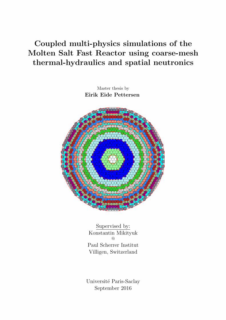
The MSFR is planned to be a 3 GWth/1.5 GWe fast-spectrum reactor optimised for simplicity andsafety. Thus, the reactor core is designed with a minimum of internal structures, as illustrated infigure 2.1. Its main characteristics are summarised in table 2.1.

Figure 2.1: Conceptual design of the MSFR [Serp et al., 2014]. It should be noted that the designis not finalised, and experiences iterative improvements as more is learned about the concept.

Parameter Value

Power 3 GWth / 1.5 GWe

Salt volume 18 m3

Salt fraction in core 50 %Number of circulation loops 16Nominal flow rate 18500 kg/s ≈ 4.5 m3/sNominal circulation time 4.0 sInlet / outlet temperature 973 K / 1073 K (700 ◦C / 800 ◦C)Blanket volume 7.3 m3

Table 2.1: Main properties of the MSFR benchmark specification.

For extracting the power generated in the MSFR, 16 independent circulation loops transfer theheat to an intermediate salt circuit which, in turn, is connected to a tertiary circuit that produceselectricity or process heat. Each of these 16 primary loops consists of a fuel pump, heat exchanger,and associated piping and instrumentation. As a result, the failure of a single circulation loop willnot reduce core cooling to the same extent had there only been a few pumps. Following a modulardesign philosophy, the circulation loops are to be constructed as separate compartments that areinstalled on the outside of the core. This ensures good accessibility and availability for maintenance,

11

as well as simple compartment replacement procedures. Surrounding the core in the radial directionare tanks in which a blanket salt with fertile material will be circulated for breeding purposes, whilereflectors cover the top and bottom. Behind the breeding blankets, a layer of absorbing material isplaced to minimise neutron irradiation of the pumps and heat exchangers. Located at the bottomof the reactor and penetrating the reflector are connections to the actively-cooled freeze plug thatwill melt and drain the core under severe accident conditions involving loss of power or overheatingof the fuel salt. Also penetrating the reflector are connections to an expansion vessel situated abovethe core and used for maintaining a constant primary pressure.

Of particular interest with the current MSFR design is the complete lack of control or safetyrods [Pioro, 2016]. Instead, the reactivity of the core is to be controlled by taking advantage ofthe negative Doppler and salt density coefficients, as well as the possibility of rapidly modifyingthe core geometry through drainage. As a result, reactivity can be controlled during nominal andaccidental operating conditions. In the former, by varying the flow of salt passing through thecore and the heat exchangers, the core temperature, and therefore reactivity, can be effectivelycontrolled. Moreover, if excessive temperatures would have to be reached for lowering reactivitysufficiently, options for reducing fuel density by the introduction of gas bubbles also exist. Duringaccidental conditions, subcriticality is achieved by transferring the fissile material to a subcriticalgeometry, i.e., the drain tanks.

Owing to the fast neutron spectrum, pictured in figure 4.1, the continuous reprocessing, and thereduction of internal structures that would otherwise absorb neutrons, the MSFR is able to runon a wide range of different fuels. This includes uranium-plutonium, uranium-thorium, and as atransmuter burning mixtures of fresh fuel and transuranic elements from used fuel in an effort toalleviate nuclear waste concerns [Fiorina et al., 2013]. The main intended purpose of the MSFR,however, is to function as a thorium breeder in a closed fuel cycle [Merle-Lucotte et al., 2011]. Witha calculated maximum breeding ratio of about 1.1 [Fiorina, 2013], one MSFR is able to producesufficient fissile material to sustain power production and generate an excess for starting up a newreactor within a relatively modest time frame. This allows for good deployment capabilities, whichare further improved by the ability to ignite MSFRs using enriched uranium and/or plutoniumstockpiles. In such closed fuel cycle, only thorium would have to be mined and supplemented tothe reactor inventory, thus greatly reducing the pressure on natural resources from using 235U as thefissile driver, as well as ensuring a fixed fuel cost undisturbed by fluctuations in electricity prices.At the other end of the fuel cycle, the back-end will benefit from a greatly diminished long-livedwaste production.

2.3.1 Salts specification

At the current stage of development, only the fuel and blanket salts of the MSFR have beencharacterised. These are both LiF-AcF4, where Ac represents an actinide, chiefly thorium oruranium for the thorium fuel cycle option. To minimise the salt melting temperature, the molefractions of LiF and AcF4 are set to 77.5 % and 22.5 %, respectively, which is the eutectic point.Sterile captures are kept low by using lithium enriched to 99.995 % in 7Li. In order to furthersimplify the computational procedures, pure 7Li is assumed in this work. For steady-state neutroniccalculations of the MSFR at a uniform temperature, this assumption led to a 33 pcm increase inreactivity, which is tolerable. The thermal-hydraulic properties of the fuel and blanket salts aresummarised in table 2.2, and were added to the TRACE source code during recent work performedat PSI [Zanetti et al., 2015]. It should be noted that in all simulations where temperatures enteredoutside of the stated validity ranges of the experimental basis, the expressions were extrapolated,with one exception. For the specific heat, the interval average cp = 1355 J/kg/K was used.

For performing the computations presented herein, a decision was made to simulate an MSFRstart-up core consisting solely of 232Th and 233U. The reactor was then made to be critical in

12

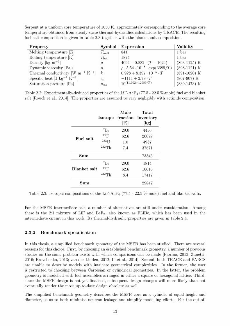
Serpent at a uniform core temperature of 1030 K, approximately corresponding to the average coretemperature obtained from steady-state thermal-hydraulics calculations by TRACE. The resultingfuel salt composition is given in table 2.3 together with the blanket salt composition.

Property Symbol Expression Validity

Melting temperature [K] Tmelt 841 1 barBoiling temperature [K] Tboil 1874 1 barDensity [kg m−3] ρ 4094− 0.882 · (T − 1024) (893-1125) KDynamic viscosity [Pa s] µ ρ · 5.54 · 10−8 · exp(3689/T ) (898-1121) KThermal conductivity [W m−1 K−1] k 0.928 + 8.397 · 10−5 · T (891-1020) KSpecific heat [J kg−1 K−1] cp −1111 + 2.78 · T (867-907) K

Saturation pressure [Pa] psat 10(11.902−12989/T ) (839-1473) K

Table 2.2: Experimentally-deduced properties of the LiF-AcF4 (77.5 - 22.5 %-mole) fuel and blanketsalt [Rouch et al., 2014]. The properties are assumed to vary negligibly with actinide composition.

IsotopeMole

fraction[%]

Totalinventory

[kg]

Fuel salt

7Li 29.0 445619F 62.6 26079

233U 1.0 4937232Th 7.4 37871

Sum 73343

Blanket salt

7Li 29.0 181419F 62.6 10616

232Th 8.4 17417

Sum 29847

Table 2.3: Isotopic compositions of the LiF-AcF4 (77.5 - 22.5 %-mole) fuel and blanket salts.

For the MSFR intermediate salt, a number of alternatives are still under consideration. Amongthese is the 2:1 mixture of LiF and BeF2, also known as FLiBe, which has been used in theintermediate circuit in this work. Its thermal-hydraulic properties are given in table 2.4.

2.3.2 Benchmark specification

In this thesis, a simplified benchmark geometry of the MSFR has been studied. There are severalreasons for this choice. First, by choosing an established benchmark geometry, a number of previousstudies on the same problem exists with which comparisons can be made [Fiorina, 2013; Zanetti,2016; Brovchenko, 2013; van der Linden, 2012; Li et al., 2014]. Second, both TRACE and PARCSare unable to describe models with intricate geometrical complexities. In the former, the useris restricted to choosing between Cartesian or cylindrical geometries. In the latter, the problemgeometry is modelled with fuel assemblies arranged in either a square or hexagonal lattice. Third,since the MSFR design is not yet finalised, subsequent design changes will more likely than noteventually render the most up-to-date design obsolete as well.

The simplified benchmark geometry describes the MSFR core as a cylinder of equal height anddiameter, so as to both minimise neutron leakage and simplify modelling efforts. For the out-of-

13

core components, axial symmetry is assumed so that no individual circulation loops are explicitlydescribed. As a result, the entire primary circuit can be modelled as a cylinder from which regionsrepresenting the blanket and absorber are cut out. The benchmark also does not characterise thepumps or heat exchangers, leaving great freedom in how to obtain the prescribed inlet temperatureand mass flow rate. Figures 2.2a and 2.2b illustrate this benchmark geometry from the side andfrom the top, respectively.

Property Symbol Expression

Melting temperature [K] Tmelt 728Density [kg m−3] ρ 2146.3− 0.4884 · TDynamic viscosity [Pa s] µ 1.81 · 10−3 · exp(1912.2/T )Thermal conductivity [W m−1 K−1] k 1.1Specific heat [J kg−1 K−1] cp 2390

Saturation pressure [Pa] psat 10(11.914−13003/T )

Table 2.4: Properties of the LiF-BeF2 (66.7 - 33.3 %-mole) intermediate salt [Benes and Konigs,2012a].

100.0

100.0

20.0

Pump

HX

Blanket

Ab

sorb

er

22

5.5

112.75 20.0

46.0

50.0 23.7

18

8.0

18

4.0

18.75

18.75

Reflector

(a) Cross-sectional side view. Note that the drawingis not to scale.

Fuel salt

AbsorberBlanket saltReflector

(b) Cross-sectional top view.

Figure 2.2: Illustrations of the axially-symmetric MSFR benchmark geometry. All dimensions arein centimetres.

All structural materials, that is, the blanket salt tank and reflector materials, have been taken to bea nickel alloy with a density of 10 g/cm3. The layer of absorbing material shielding the pumps andheat exchangers is boron carbide with a density of 2.52 g/cm3, while the heat exchangers have beenmodelled consisting of Hastelloy-N. Table 2.5 lists the elemental compositions of these materials.

Element B C Al Si V Cr Mn Fe Ni Mo W

A.f. [%]Absorber 80 20 - - - - - - - - -Structure - - 0.3 - - 7.0 - - 67.7 - 25.0

W.f. [%] HXs - 0.06 ≤0.5 ≤1 ≤0.5 7 ≤0.8 ≤4 71 16 ≤0.5

Table 2.5: Elemental composition of the various materials used in the modelling of the MSFR[Haynes International, 2015; Aufiero, 2014]. A.f. refers to atomic fraction, while w.f. denotesweight fraction.

14

3 Computational tools

Three distinct tools were used over the course of this project: The thermal-hydraulics system codeTRACE developed by the NRC, the Monte Carlo neutronics code Serpent (v.2.1.26) under activedevelopment at the VTT Technical Research Centre of Finland, and the deterministic neutronicssolver PARCS from Purdue University. In this chapter each of these codes will be briefly presented.Particular focus will be put on the underlying equations that are being solved in an attempt tounderstand the assumptions and simplifications that inevitably limit the accuracy of the solutionproduced. In addition to this, the particularities of the different implementations of the benchmarkproblem in each tool are described. Lastly, the methodology for combining these three separatetools into a single, coupled multi-physics solver is covered.

3.1 TRACE

The TRAC/RELAP Advanced Computational Engine is a thermal-hydraulics system code thatsolves the conservation of mass, momentum, and energy for two-phase flows subjected to internaland external heat transfer using finite volume numerical methods. It does so for 0D, 1D, and 3Dgeometries, and generally on fairly coarse computational meshes over which the problem variablesare averaged. Integral quantities are then represented in mesh centre points, while those withdirections are stated on the mesh boundary corresponding to the direction of the quantity. Forinstance, the velocity component in an arbitrarily defined x direction within a cell will be specifiedon the face of the cell whose normal vector points in the x direction. This is known as a staggeredmesh [Patankar, 1980]. The thermal-hydraulic problem to be solved is formulated through theuse of built-in components defined within TRACE. These include components representing one-dimensional pipes, pumps, and plenums, three-dimensional vessels, as well as solid heat structuresand distributed power components. All components that carry fluid can then be subdivided intocells of arbitrary sizes. The specification of three-dimensional cells illustrate one restriction relatedto the usage of TRACE, as users can only choose between Cartesian or cylindrical geometries.

3.1.1 Principal equations

Within all flow-carrying components, the aforementioned equations are solved. The exact formu-lations are [NRC, 2007] (c.f. the nomenclature for description of symbols)

∂ρ

∂t+∇ · ρu = 0, (3.1)

for the conservation of mass,

∂(ρu)

∂t+∇ · (ρu · u) +∇p = fw + ρg, (3.2)

15

for the conservation of momentum, and

∂[ρ(e+ u2/2)]

∂t+∇ · [ρ(e+

p

ρ+ u2/2)] = qw + qf + ρg · u+ fw · u, (3.3)

for the conservation of energy. In these equations, Reynolds averaging is applied to each calculatedquantity so as to ignore small temporal fluctuations and obtain time-averaged behaviour. Thus,calculated quantities are averaged both in space and time. TRACE also contains a similar set ofequations describing the gas state of the fluid. However, since the margin-to-boiling for the moltensalts in the MSFR is substantial, these equations as well as the terms describing interfacial exchangeof mass, momentum, and energy are not resolved in the simulations presented herein. That beingsaid, while molten salt boiling is out-of-scope at the current stage of development of the MSFRdesign, it is clearly a topic that will demand attention as the concept matures. Moreover, theprimary salt will contain bubbles of fission product gases and tritium, among other things, thatwill require salt-gas flow equations to resolve.

Also neglected in the energy conservation equation above is the term describing heat conductionwithin the fluid. In TRACE, the inclusion of this term is activated or deactivated through userinput. Since the salts used in the MSFR typically have relatively large Prandtl numbers [Fiorina,2013] so that convective heat transfer dominates, the option has been deactivated.

The wall friction force term, fw, deserves scrutiny. It describes frictional forces on pipe flow and isdefined as

fw = Cwu|u|, (3.4)

where the wall drag coefficient is given as

Cw = kw2ρ

Dh, (3.5)

and kw = kw(Re,Dh, δ) is the Churchill correlation friction factor [NRC, 2007]. Not included in thisfriction term, nor anywhere else in the above formulations, are viscous shear stresses or turbulenceeffects such as those included in the k-ε turbulence model or similar models. These terms areneglected in TRACE. As a consequence, the code can not be expected to accurately recreate flowbehaviour that is significantly affected by turbulence, including large, open flow regions that exhibitrecirculation zones. Note that this point is of particular importance for the results presented in thebelow, as turbulence effects are very much present in the MSFR core where the Reynolds numbermay reach 106 [van der Linden, 2012].

An additional assumption is made in TRACE for calculating the convection term of the momentumconservation equation, ∇· (ρu ·u), in multi-dimensional geometries. When cell surface velocities onthe staggered mesh are used to estimate the momentum flux at cell centres, momentum convectionis assumed to only be performed by the velocity component in the same direction as the momentumflux component being calculated. In other words, cross-derivative terms of the divergence operatorare ignored. The severity of this approximation varies with cell size, as well as the amount of flowmixing in the core.

In this work, the entire primary circuit of the MSFR was modelled within one three-dimensional,axially symmetric vessel component using the cylindrical geometry option. When using vesselcomponents, it is possible to define the hydraulic diameter for each cell in both radial and axialdirections. By taking advantage of the functional dependence of the friction factor defined inequation 3.5 (it can be shown to decrease uniformly with increasing Dh), artificial drag can be

16

introduced away from physical walls in order to alleviate the lack of viscous shear stresses withinthe fluid in the MSFR core region. In doing this, the use of a uniform hydraulic diameter in thesame direction is beneficial from the point of view of numerical stability. Additional friction closeto walls can then be added by means of additive-friction-loss coefficients, specified as user input toTRACE, for a more realistic wall drag behaviour. Otherwise, no slip velocity boundary conditionsare assumed by TRACE at the walls of vessel components.

The last field equations to be solved by TRACE calculates the amount and distribution of DNPsand decay heat in the problem geometry. For DNP group j, the balance equation reads

∂(ρcj)

∂t+∇ · (uρcj) = ∇ · (Dm,jρ∇cj) + ρ(βjn− λjcj), (3.6)

where the molecular diffusivity Dm,j = 1.0 ·10−3 m2s−1 for all the groups and for the decay heat inaccordance with [Fiorina, 2013] and [Zanetti, 2016], and j ∈ {1, 9}, where 9 indicates decay heat. Nodifference to the balance equation is made when calculating a group of DNPs or decay heat, as theunderlying physical processes at work are identical. The group delayed neutron fractions and decayconstants were calculated with Serpent using the iterated fission probability method [Leppanenet al., 2014], except for the values for decay heat which were adopted from [Zanetti, 2016]. Theyare all reported in table 3.1. Compared to traditional DNP balance equations, two additional termsdescribing convective and diffusive transport of DNPs are introduced in equation 3.6. The equationset is solved by extracting velocity and temperature fields from TRACE in order to evaluate theconvection and material properties, respectively. Also part of MSR phenomenology but neglectedin the above formulation is DNP extraction through precipitation and deposition. This has beenshown to affect less than about 1 % of DNPs [Doligez, 2010].

Group number j βj [pcm] λj [s−1]

1 22.3 0.01252 45.3 0.02833 38.8 0.04254 60.8 0.1335 96.9 0.2926 14.8 0.6667 20.6 1.638 4.49 3.55

Decay heat 253 0.214

Table 3.1: Delayed neutron precursor groups utilised in TRACE calculations.

In addition to the presented field equations, TRACE employs routines for solving heat conductionproblems in heat exchangers or through solid heat structures such as fuel pins. These equationsare coupled to the field equations above by the term qw in equation 3.3.

3.1.2 Primary circuit model

The flow path of the MSFR primary circuit has been defined within the aforementioned vesselcomponent in TRACE. This was accomplished by taking advantage of the porous media func-tionality offered by TRACE in vessel components to simplify the implementation of channel-likeLWR vessels. Porous media functionality allows the user to specify volume fractions taken up bynon-fluid (typically solid, internal structures) in each mesh cell, and surface area fractions that areblocked for the fluid on all cell faces. As such, regions of the cylinder-shaped vessel component

17

can be rendered unavailable for the molten salt to enter, and the fluid can thus be directed alongthe desired flow path. The isolated region represents the blanket and absorber of the benchmarkgeometry. Although detailed modelling of these parts would be viable, and likely would improvethe accuracy of transients particularly sensitive to the large heat reservoirs represented by thesecompartments, no such modelling has been attempted in this thesis. This simplification is justifiedin section 4.1.2.

On the top of the vessel component, attached to the outermost, torus-shaped cell is a connectionthat leads to an expansion chamber. Pressure control of the primary is obtained by imposing aboundary pressure at the end of this connection. In transient simulations comparatively cold saltdevoid of DNPs enters the primary circuit through from the expansion chamber when the fuel saltcontracts. The connection is therefore placed at the core outlet to reduce the neutronic interferenceof this scenario.

3.1.3 Heat exchanger and pump models

The primary heat exchanger has been modelled in accordance with the recommendations made ina previous study on the topic of MSFR heat exchangers performed at PSI [Ariu, 2014]. Table 3.2lists the main properties of this heat exchanger.

General properties

Type Counterflow printed circuitPrimary side salt LiF-AcF4

Secondary side salt LiF-BeF2

Length [m] 1.17Channel shape Half-circle

Channel diameter [mm] 1.7Channel pitch [mm] 1.9Number of channels 253356

Construction material Hastelloy-N

Primary side properties

Inlet temperature [K] 1023Outlet temperature [K] 923

Salt velocity [m/s] 1.17Pressure loss [bar] 4.1

Secondary side properties

Inlet temperature [K] 863Outlet temperature [K] 943

Salt velocity [m/s] 2.00Pressure loss [bar] 5.2

Table 3.2: Main properties of the implemented primary heat exchanger model, from [Ariu, 2014].Note that the properties listed describe only one of 16 identical heat exchangers distributed aroundthe MSFR core, and had to be scaled up for use in the axially symmetric benchmark geometry.

On the secondary side, the inlet mass flow rate, temperature, and outlet pressure were imposed inorder to obtain the characteristics in table 3.2. Since the properties of the channels were designedfor 1/16th the total flow of the MSFR, provisions were made to accommodate the full flow of theaxially symmetric model. Specifically, the number of channels and secondary mass flow rate wasincreased by a factor of 16.

The implemented heat exchanger model stands in contrast to implementations in previous works,

18

where some simplifications are commonly applied [Zanetti et al., 2015; Fiorina, 2013]. Most im-portantly, in both cited MSFR models the secondary side temperature is constant and imposed.Heat exchange is then determined by a flow-dependent expression for the heat transfer coefficientbetween primary and secondary sides.

In TRACE, pumps are modelled as centrifugal pumps in which a rotating impeller imparts mo-mentum to the fluid. The amount of momentum depends on the pump curves used, in addition tothe rated torque, rated head, rated volumetric flow, rated fluid density, and rotational velocity ofthe pump. Throughout this project, all but the latter variables have been set to constant values,and the rotational velocity has been used to vary the primary mass flow. Table 3.3 lists the refer-ence values that have been used to evaluate momentum from a semiscale pump curve built in toTRACE. Also note that the pump is situated above the heat exchanger despite concerns regardingdegraded natural circulation, high temperatures, and large thermal stresses in the pump. Thisdesign choice follows the convention of the MSFR conceptual drawings in literature [Brovchenko,2013; Li et al., 2014; Rouch et al., 2014], and deviates from the two other MSFR models previouslyused for comparison.

Rated head [m2 s2] 50Rated torque [Pa m3] 3000

Rated volumetric flow [m3 s−1] 1.0Rated density [kg m−3] 4125

Table 3.3: Reference values used for evaluating the amount of momentum imparted by the primarycentrifugal pump.

Figure 3.1: MSFR model implemented in Serpent. The different shades of green correspond todifferent regions in which cross sections were generated. Only the cross sections from the centralcore region are used in PARCS. The remaining colours represent: orange - blanket, dark grey -absorber, light grey - reflector and blanket casing.

3.2 Serpent

Serpent is a continuous-energy Monte Carlo neutronics code capable of solving the neutron trans-port problem by tracking individual neutrons within the problem geometry and using stochastic

19

procedures to determine the chain of events for each neutron. It has been under active developmentat the VTT Technical Research Centre of Finland since 2004, where it was initially conceived as atool to simplify group constant generation in a high-fidelity Monte Carlo environment. Since then,Serpent has seen a steady growth of its user base, that now encompasses more than 500 registeredindividuals in 155 organisations located in 37 countries around the world. This success is not only aresult of the simplified cross section generation procedures, but also its high-performance parallel-computation capabilities and user-friendly usage, as well as thorough validation with establishedcodes like MCNP [X-5 Monte Carlo Team, 2003] and experiments.

The MSFR benchmark implementation in Serpent is illustrated in figure 3.1. As in the TRACEmodel, the geometry is axially-symmetric. Since the heat exchangers and pumps are located behindthe neutron absorber where their neutronic importance is severely reduced, their inclusion in theSerpent model has been neglected.

This Serpent model of the MSFR has been used to generate cross sections at a number of differentfuel temperatures and densities. By varying these two parameters separately, both individualDoppler and fuel density reactivity coefficients and the combined temperature coefficient could bedetermined.

Furthermore, reference cross sections were generated at a uniform temperature of 900 K, as well ascross section derivatives to be used by the coupled code in transient analyses. Owing to the fastneutron spectrum of the MSFR, the Doppler cross section derivative for an arbitrary macroscopiccross section x was calculated with [Waltar et al., 2012]

(∂Σx

∂T

)T

=Σx,T1 − Σx,T2

lnT1 − lnT2, (3.7)

while for the fuel density derivatives,

(∂Σx

∂T

)ρ

=Σx,T1 − Σx,T2

T1 − T2, (3.8)

was used. Note that the reference cross sections were calculated at the temperature of the micro-scopic cross section libraries used by Serpent closest to the core average temperature (i.e., at 900K) rather than at the core average temperature itself (about 1030 K) in order to avoid discrepan-cies introduced by the internal cross section interpolation in Serpent. The derivatives were thencalculated using the macroscopic cross sections generated at 900 K and 1200 K.

3.3 PARCS

The Purdue Advanced Reactor Core Simulator is a spatial neutron kinetics solver that calculatesthe solution to the multi-group neutron diffusion equation, formulated as

1

vg

dφgdt

= ∇ · (Dg∇φg)− Σt,gφg +1

keffχp,g

∑g′

νp,g′Σf,g′φg′ + χd,g∑j

λjcj +∑g′

Σg′→gφg′ (3.9)

for energy group g, where p denotes prompt neutrons, d delayed neutrons, and j iterates theDNP groups. It does so by discretising the temporal variable according to the theta method, andthe spatial variables in a coarse mesh finite difference (CMFD) framework. The resulting finitedifference formulation is refined by updating the nodal coupling coefficients by means of a hybrid

20

nodal expansion and analytical nodal method. For solving steady-state conditions, the eigenvalueproblem is then solved using the Wielandt eigenvalue shift method. In transient conditions, thesteady-state is first solved and the computed neutron multiplication factor used to make criticalthe initial state of the transient. A fixed-source problem is established next and solved repeatedlyfor both the main CMFD equations and local two-node supplementary equations at every pointin time of the transient. The use of a diffusion equation formalism is expected to be appropriatefor describing the neutron flux present in the large, homogeneous core of the MSFR, provided thata sufficient number of energy groups is defined. That being said, some discrepancies in the fluxshape can be expected close to the core boundaries where an albedo boundary condition is used toreproduce the keff found by Serpent. Specifically, the albedo value set by the user is defined as

ax =J(x)

φ(x)

∣∣∣∣x=xsurface

=1

2

(1− αx1 + αx

), where (3.10)

αx =Jin,x

Jout,x, (3.11)

and xsurface signifies the radial, top, or bottom boundary. For the radial discretisation in PARCSillustrated in figure 3.2, a value of ax = 0.095 was used on all three boundaries.

Core geometry modelling in PARCS is achieved by defining either square fuel assemblies associatedwith Western-type LWR cores, or hexagonal assemblies for VVER-type cores. Thus, for couplingpurposes, the number of assemblies specified in PARCS must be high to obtain a good approxi-mation of the cylindrical mesh used in TRACE. Since fewer hexagonal assemblies are required toobtain a good approximation of a circle than squares, the hexagonal shape was chosen to reducethe computational burden. Figure 3.2 shows an example of a radial mesh used in PARCS. In theaxial direction, the discretisation from TRACE could be directly adopted.

Collapsed and spatially averaged macroscopic cross sections generated in the core region by Serpentwere provided to PARCS. For this purpose, a six-group energy discretisation was adopted from pre-vious studies on the MSFR neutronic behaviour [Zanetti, 2016; Fiorina, 2013; Aufiero, 2014]. Table3.4 recalls the particular discretisation. In addition to this, cross section derivatives were calculatedfrom Serpent calculations performed at 900 K and 1200 K, corresponding to the temperatures ofthe microscopic cross section libraries used by Serpent. By providing a reference fuel and coolanttemperature, PARCS evaluates the differences with regards to current cell temperature and useslinear extrapolation to continuously update the cross sections throughout the transient calculation.Since PARCS also receives the DNP concentrations, ck from TRACE, it is able to solve equations3.9 for the neutron group fluxes and return the associated power distribution.

Group number 1 2 3 4 5 6

Lower boundary [MeV] 2.231 4.979·10−1 2.479·10−2 5.531·10−3 7.485·10−4 0

Table 3.4: Lower boundary of the energy groups utilised in PARCS calculations.

3.4 Coupling methodology

The coupling between TRACE and PARCS is accomplished by mapping thermal-hydraulic cells inTRACE to corresponding neutronic nodes in PARCS. One such map of radial nodes is illustrated infigure 3.2. In the axial direction, one-to-one mapping is used. Cell fluid temperatures and densitiesare then transferred from TRACE to PARCS through an interprocess communication protocol.Moreover, source code extensions to allow for the transfer of DNP concentrations have been imple-mented at PSI, and further extended to be compatible with vessel components within this project.

21

From the temperature and DNP distributions, PARCS calculates the cell-wise power distribution,which is then returned to TRACE. Originally, the calculated power distribution is returned to solidheat structure components in TRACE representing the fuel rods in LWRs. Additional modifica-tions to the TRACE source code have been made at PSI in the past to ensure that the returnedpower is deposited directly in to the coolant [Kim, 2015], as is the case for liquid-fuelled reactors.

Figure 3.2: The radial discretisation of the MSFR core (inner salt circle in figure 2.2b) in PARCSoverlaid with the TRACE discretisation (red, circular lines) illustrating the coupled regions thatmap variables from one code to the other. In total, 1285 radial cells have been used in PARCS tocover the 14 radial core cells in TRACE.

Throughout the coupled calculation the two codes are run in parallel, and the aforementioned in-formation exchange procedure is performed at every time step. This coupling approach is calledoperator splitting, and has the advantage of being very intuitive, and allowing two well-establishedand thoroughly validated codes to operate together in a coupled manner. Conversely, operatorsplitting is time consuming as one code always has to await the response of the other, and suf-fers from issues of numerical stability related to the control of the size of time steps [Pope andMousseau, 2009]. In TRACE, a variable time step control procedure determines at any time theappropriate time step size subjected to upper and lower boundaries imposed by the user. To reducecomputational times, this time-differencing procedure is allowed to exceed the material Courantlimit condition that relates the time step size to the characteristic cell size and fluid velocity [NRC,2007]. Generally, this routine was found to be unreliable for coupled calculations, and a strictrestriction on the upper time step size had to be given to ensure stability.

22

4 Results

Two main categories of simulations have been performed over the course of this project. First,the neutronic and thermal-hydraulic steady-states of the MSFR were separately investigated usingSerpent and TRACE, respectively. Of these, Serpent was run first in order to determine thepower distribution and DNP properties later provided to TRACE. Furthermore, macroscopic crosssections generated by Serpent were used in the standalone PARCS code, and the resulting neutronicsolution has been compared with that of Serpent. Second, TRACE and PARCS have been coupledin order to study transient behaviour. Specifically, transients describing primary pump over-speed,primary circuit over-cooling, loss of heat sink, and loss of flow scenarios have been investigated.

Results from both the steady-state and transient simulations are presented in the following. Sinceobtaining steady-state simulations in both TRACE and PARCS are prerequisites for performingcoupled calculations, it is natural to begin with the steady-state. In both cases, the obtainedresults have been compared with results from other tools where data is available. This includesan ERANOS-based code [Fiorina, 2013; Rimpault et al., 2002] used for steady-state neutronicassessments, and a CFD tool [Fiorina, 2013] based on the physics simulator COMSOL [COMSOL,2012] and the DNP-extended TRACE code with a simplified point-kinetics routine (hereby referredto as TRACE-PK [Zanetti, 2016]), both used for steady-state thermal-hydraulic and transientanalyses.

It should be noted that because of the interconnected structure of the computational proceduresfollowed, almost all presented results will have some dependency on the microscopic cross sectionlibrary providing data to Serpent. Unless otherwise specified, the JEFF 3.1.1 library [Santamarinaet al., 2009] has been used.

4.1 Steady-state behaviour

The steady-state behaviour of the MSFR has been characterised both in terms of neutronics andthermal-hydraulics, in an uncoupled manner. There are two main incentives for doing this. First,the steady-state solution is required in order to initialise the coupled tool that serves as the focalpoint of this thesis. Second, the steady-state analysis highlights a number of characteristics of MSRsin general, and the MSFR in particular. Thus, the presented results and associated discussion aimsat clarifying and expanding some of the concepts previously introduced, and provide context forinterpreting the transient results that follow.

For performing steady-state simulations, some assumptions had to be made that limit the accuracyof the obtained results. Most importantly, the neutronic study using Serpent was performed atuniform fuel salt temperatures, and the thermal-hydraulics were studied with an imposed, time-invariant power distribution obtained from the uniform-temperature Serpent model. As a result,in terms of thermal-hydraulics, discrepancies can be expected compared to the COMSOL andTRACE-PK tools that both make use of a power distribution calculated by means of a spatialneutron diffusion approach. Justification for introducing this additional source of discrepancy lies

23

in that the main focus of this work is the assessment of the coupled TRACE-PARCS tool. Separate-physics simulations of the thermal-hydraulic steady-state behaviour are merely a necessary step forinitialising the transient simulations performed with the coupled tool, for which this limitation islifted.

In the following, the neutronic steady-state will first be described. This includes results obtainedwith Serpent, as well as comparisons with standalone PARCS and similar results from literature.Thereafter, a brief study of nominal power deposition in the blanket is presented in an attempt tojustify the choice of neglecting the blankets in the thermal-hydraulic model. Finally, the TRACEsteady-state solution will be presented and compared with the CFD-based COMSOL and TRACE-PK solutions where possible.

4.1.1 Neutronics

The steady-state neutronic results presented in the below were obtained by following a particularcomputational procedure. First, Serpent was used to calculate keff at a uniform temperaturecorresponding to a preliminary estimate of the core average temperature of 1030 K.5 The amountof fissile material was then adjusted in order make the reactor critical at this temperature. Thisresulted in a 1 % increase compared to the benchmark reference fissile inventory [Merle-Lucotteet al., 2011], but also a 2 % decrease compared to the values reported in [Fiorina, 2013]. Next,macroscopic cross sections were generated from simulations at temperatures of 900 K (used asreference) and 1200 K (for calculating derivatives). At the latter temperature two sets of simulationswere performed in order to separate the effects from changes of fuel temperature and fuel density.At the same time, keff was calculated in order to evaluate the two feedback coefficients, as well asthe combined temperature coefficient.

By following the procedure outlined in [Ghasabyan, 2013], cross sections calculated by Serpent canbe introduced into PARCS. This opens up for two distinct methods of performing PARCS calcu-lations at different core temperatures, namely (a) to use directly cross sections generated at thedesired temperature, or (b) using reference cross section together with cross section derivatives.Only the second method is compatible with spatial temperature distributions, and has thereforebeen used in the following. The only exception to this rule was made when calibrating the PARCSboundary conditions to correspond with results from Serpent. That is, the albedo condition wasadjusted to yield a critical core at the uniform core temperature of 1030 K using Serpent cross sec-tions generated at 1030 K. Then, method b could be used to evaluate keff at different temperaturesand compare the resulting temperature coefficients with Serpent, which was adopted as reference.The results are reported in tables 4.1 and 4.2, for three different numbers of radial cells in PARCS,together with values from ERANOS where appropriate.

Code keff, 1030 KDiff. wrt.

Serpent [pcm]keff, 1200 K

Diff. wrt.Serpent [pcm]

Serpent 1.00000 0 0.98716 0PARCS, 2929 cells 0.99917 -83 0.98633 -83PARCS, 1891 cells 0.99917 -83 0.98625 -91PARCS, 1285 cells 0.99917 -83 0.98624 -92

Table 4.1: Selected values of keff as calculated by the different tools. The number of cells in PARCSrefer to radial cells (c.f. figure 3.2).

5This estimate was in turn obtained by using a first-approximation cosine-shaped power distribution in TRACE.

24

Code αD [pcm/K] αρ [pcm/K]αD + αρ[pcm/K]

αT [pcm/K]

Serpent -3.88 ± 0.02 -3.48 ± 0.02 -7.36 ± 0.03 -7.27 ± 0.02PARCS, 2929 cells -3.87 -3.54 -7.41 -7.58PARCS, 1891 cells -3.87 -3.59 -7.45 -7.62PARCS, 1285 cells -3.87 -3.59 -7.46 -7.63

ERANOS -4.19 -3.10 -7.29 N/A

Table 4.2: Reactivity coefficients as calculated by different tools. The number of cells in PARCSrefer to radial cells (c.f. figure 3.2). See the nomenclature for explanation of symbols. For allbut the bottom row, the coefficients have been calculated as α = (k2

eff − k1eff)/(k1

eff · ∆T ), withk1

eff = keff(900K), k2eff = keff(1200K), and ∆T = (1200− 900) K. In the ERANOS calculations, 973

K and 1073 K were used in place of 900 K and 1200 K [Fiorina, 2013].

A few conclusions can be drawn from tables 4.1 and 4.2. First, differences in keff between PARCSand Serpent are on the order of 100 pcm, and do not vary much with the number of radial cellsin PARCS. Second, the assumption that the overall temperature reactivity coefficient, αT , is asuperposition of the Doppler and fuel density coefficients appears good with discrepancies on theorder of 1-2 %. Third, the discrepancies between PARCS and Serpent for the summed Doppler anddensity coefficients (which are the ones used in PARCS)) are also about 1-2 %, and only modestimprovements are obtained with considerably more radial cells. This could likely be improved byincreasing the number of zones in which Serpent produce cross sections for PARCS. However, thatis not done here as these results are deemed acceptable for the purpose of verifying code behaviour.Also, in order to reduce computing times without sacrificing much accuracy, the roughest radialmesh is chosen in PARCS for the continued analysis. Fourth, both PARCS and Serpent results areconsistent with those from ERANOS. The discrepancy in the Doppler coefficient is likely due tothe aforementioned difference in fuel composition [Fiorina, 2013], while the fuel density coefficientcould be related to the extrapolation of the salt density used when calculating keff at 1200 K (c.f.table 2.2). In the ERANOS calculations this was avoided by calculating the coefficients between973 K and 1073 K, which, on the other hand, introduces uncertainty related to microscopic crosssection interpolation.

10-5 10-4 10-3 10-2 10-1 100 101

Energy [MeV]

0.00

0.05

0.10

0.15

0.20

0.25

Norm

alis

ed f

lux p

er

leth

arg

y [

AU

]

PARCS (6g)

Serpent

Serpent (6g)

ERANOS (6g)

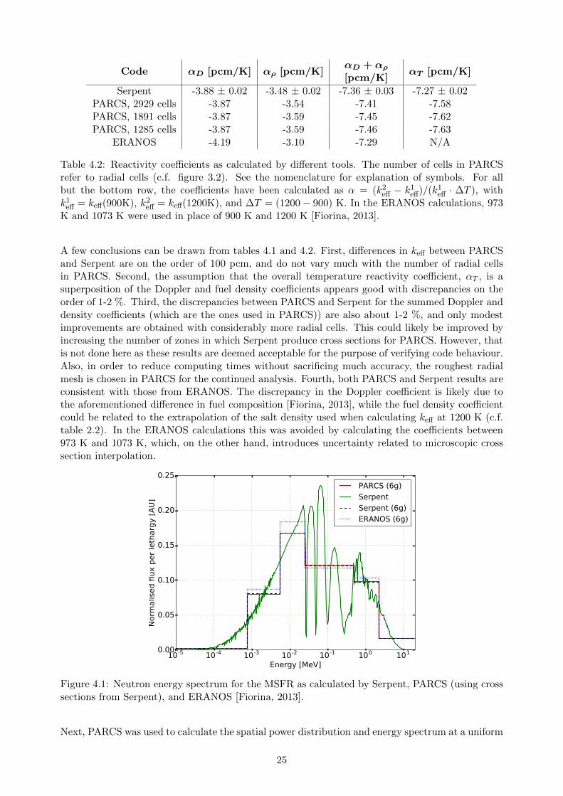
Figure 4.1: Neutron energy spectrum for the MSFR as calculated by Serpent, PARCS (using crosssections from Serpent), and ERANOS [Fiorina, 2013].

Next, PARCS was used to calculate the spatial power distribution and energy spectrum at a uniform

25

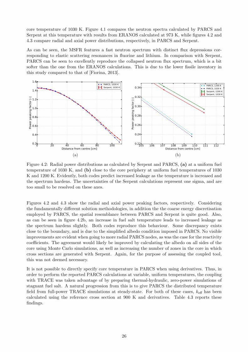
core temperature of 1030 K. Figure 4.1 compares the neutron spectra calculated by PARCS andSerpent at this temperature with results from ERANOS calculated at 973 K, while figures 4.2 and4.3 compare radial and axial power distributions, respectively, in PARCS and Serpent.

As can be seen, the MSFR features a fast neutron spectrum with distinct flux depressions cor-responding to elastic scattering resonances in fluorine and lithium. In comparison with Serpent,PARCS can be seen to excellently reproduce the collapsed neutron flux spectrum, which is a bitsofter than the one from the ERANOS calculations. This is due to the lower fissile inventory inthis study compared to that of [Fiorina, 2013].

0 20 40 60 80 100Distance from centre [cm]

0.2

0.4

0.6

0.8

1.0

1.2

1.4

1.6

Pow

er

peaki

ng f

act

or

[-]

PARCS, 1030 K

Serpent, 1030 K

(a)

105 106 107 108 109 110 111 112Distance from centre [cm]

0.22

0.24

0.26

0.28

0.30

0.32

0.34

Pow

er

peaki

ng f

act

or

[-]

PARCS, 1200 K

PARCS, 1030 K

Serpent, 1200 K

Serpent, 1030 K

(b)

Figure 4.2: Radial power distributions as calculated by Serpent and PARCS, (a) at a uniform fueltemperature of 1030 K, and (b) close to the core periphery at uniform fuel temperatures of 1030K and 1200 K. Evidently, both codes predict increased leakage as the temperature is increased andthe spectrum hardens. The uncertainties of the Serpent calculations represent one sigma, and aretoo small to be resolved on these axes.

Figures 4.2 and 4.3 show the radial and axial power peaking factors, respectively. Consideringthe fundamentally different solution methodologies, in addition the the coarse energy discretisationemployed by PARCS, the spatial resemblance between PARCS and Serpent is quite good. Also,as can be seen in figure 4.2b, an increase in fuel salt temperature leads to increased leakage asthe spectrum hardens slightly. Both codes reproduce this behaviour. Some discrepancy existsclose to the boundary, and is due to the simplified albedo condition imposed in PARCS. No visibleimprovements are evident when going to more radial PARCS nodes, as was the case for the reactivitycoefficients. The agreement would likely be improved by calculating the albedo on all sides of thecore using Monte Carlo simulations, as well as increasing the number of zones in the core in whichcross sections are generated with Serpent. Again, for the purpose of assessing the coupled tool,this was not deemed necessary.

It is not possible to directly specify core temperature in PARCS when using derivatives. Thus, inorder to perform the reported PARCS calculations at variable, uniform temperatures, the couplingwith TRACE was taken advantage of by preparing thermal-hydraulic, zero-power simulations ofstagnant fuel salt. A natural progression from this is to give PARCS the distributed temperaturefield from full-power TRACE simulations at steady-state. For both of these cases, keff has beencalculated using the reference cross section at 900 K and derivatives. Table 4.3 reports thesefindings.

26

120 140 160 180 200 220Distance from bottom [cm]

0.2

0.4

0.6

0.8

1.0

1.2

1.4

1.6

Axia

l peaki

ng f

act

or

[-]

PARCS, 1030 K

Serpent, 1030 K

Figure 4.3: Axial power distribution as calculated by PARCS and Serpent at a uniform coretemperature of 1030 K. The uncertainties of the Serpent calculations represent one sigma, and aretoo small to be resolved on these axes.

Temperature distribution Tcore, avg. [K] keff

Uniform, 1030 K cross sections 1030 1.0Uniform, derivatives 1030 0.99917

Distributed 1034 1.00032

Table 4.3: Neutron multiplication factors calculated by PARCS with different cross section andtemperature input.

As can be seen, differences on the order of 80 pcm are observed when cross section interpolationwith derivatives is used. This indicates a more complex cross section dependency with temperature,but could also be influenced by the microscopic cross section interpolation in Serpent. The changeto distributed temperatures introduces 115 pcm of positive reactivity despite increasing the coreaverage temperature by about 4 K. Much of the reason for this is the existence of a localised regionof high salt temperatures outside of high neutron importance regions in the centre of the core (c.f.chapter 4.1.3).

A final note is offered on the use of microscopic cross section libraries in Serpent. AlthoughJEFF 3.1.1 is used exclusively in this thesis, keff at 900 K was calculated using the ENDF/B-VIIlibrary [Chadwick et al., 2011] with Serpent. A difference of more than 1000 pcm was found, withENDF providing the more conservative estimate. This is consistent with other reports of importantdependency on cross section libraries, primarily due to uncertainties in the (n, γ) capture crosssection of 233U [Aufiero, 2014].

4.1.2 Blanket behaviour

The amount and distribution of power deposited in the blanket during steady-state operation wasinvestigated in order to advise the thermal-hydraulic modelling of the MSFR primary circuit. Inparticular, the study was aimed at determining the importance of including a detailed blanketmodel for the steady-state thermal-hydraulic analysis.

Two main phenomena are responsible for heating the blanket. At beginning of life, when only

27

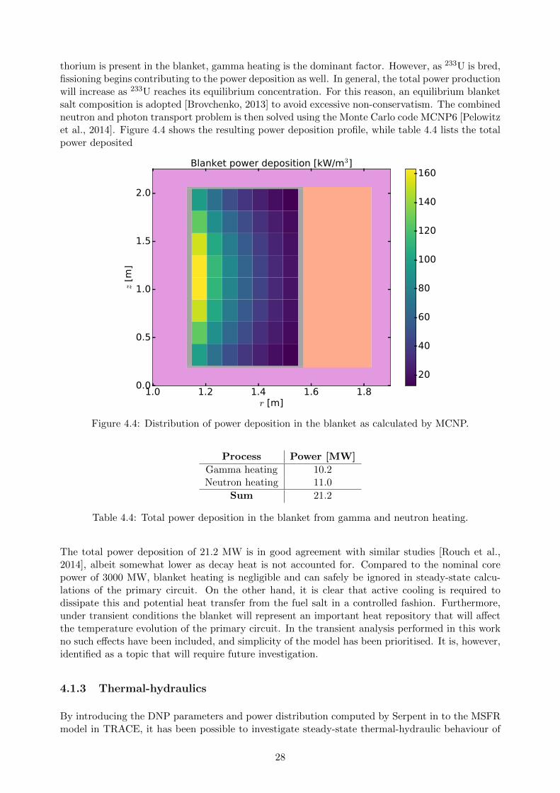
thorium is present in the blanket, gamma heating is the dominant factor. However, as 233U is bred,fissioning begins contributing to the power deposition as well. In general, the total power productionwill increase as 233U reaches its equilibrium concentration. For this reason, an equilibrium blanketsalt composition is adopted [Brovchenko, 2013] to avoid excessive non-conservatism. The combinedneutron and photon transport problem is then solved using the Monte Carlo code MCNP6 [Pelowitzet al., 2014]. Figure 4.4 shows the resulting power deposition profile, while table 4.4 lists the totalpower deposited

1.0 1.2 1.4 1.6 1.8r [m]

0.0

0.5

1.0

1.5

2.0

z [m

]

Blanket power deposition [kW/m3]

20

40

60

80

100

120

140

160

Figure 4.4: Distribution of power deposition in the blanket as calculated by MCNP.

Process Power [MW]

Gamma heating 10.2Neutron heating 11.0

Sum 21.2

Table 4.4: Total power deposition in the blanket from gamma and neutron heating.

The total power deposition of 21.2 MW is in good agreement with similar studies [Rouch et al.,2014], albeit somewhat lower as decay heat is not accounted for. Compared to the nominal corepower of 3000 MW, blanket heating is negligible and can safely be ignored in steady-state calcu-lations of the primary circuit. On the other hand, it is clear that active cooling is required todissipate this and potential heat transfer from the fuel salt in a controlled fashion. Furthermore,under transient conditions the blanket will represent an important heat repository that will affectthe temperature evolution of the primary circuit. In the transient analysis performed in this workno such effects have been included, and simplicity of the model has been prioritised. It is, however,identified as a topic that will require future investigation.

4.1.3 Thermal-hydraulics

By introducing the DNP parameters and power distribution computed by Serpent in to the MSFRmodel in TRACE, it has been possible to investigate steady-state thermal-hydraulic behaviour of

28

the benchmark MSFR problem, in addition to the DNP distribution. In the following, some remarkson the model and methodology will be given, followed by the presentation of selected results. Theseinclude the steady-state velocity, temperature, and pressure fields, as well as DNP distributionsand the effective delayed neutron fraction, βeff (which are not thermal-hydraulic results, per se, butcomputed by the thermal-hydraulic code).

Due to the simplified coarse-mesh approach utilised by TRACE, it has been of particular interestto compare the obtained results with those from a more complex, CFD-based solver implementedin COMSOL. This tool is explained in detail in [Fiorina, 2013]. Some model adjustments wererequired in order to facilitate this comparison. Specifically, the inlet and outlet temperature of thecore were aligned with those of the COMSOL solution, which did not correspond exactly to thebenchmark values. Most importantly, the temperature rise in the core was close to 90 K instead of100 K. Furthermore, it was found that adding artificial friction in the core region as described inchapter 3.1 improved mixing and thus the distribution of heat. As such, the core peak temperaturecould be made the same as in the COMSOL model.

Steady-state was obtained in approximately ten minutes on a single 2.6 GHz Intel Xeon processor.Most of this time was taken up by the convergence of the DNPs - the half-life of the longest-livedgroup is about 50 s, so simulation times had to exceed five times this as a minimum. The thermal-hydraulics solution in itself converged much faster, in the order of tens of seconds. Initially, effortswere directed towards modelling the full three-dimensional geometry in TRACE by subdividing thecylindrical mesh into 16 azimuthal sectors representing the individual recirculation loops. This wasdesirable as it would allow for the simulation of asymmetrical transients such as single pump failure.However, computational times were found to scale significantly with model complexity, especiallyfor the coupled tool, to the point that simulations on a single processor was unfeasible. It shouldbe noted that parallelisation is possible in TRACE by decomposing the model into zones that aresolved on separate processors, but the process is not straightforward and was not attempted in thisthesis work.

An important aspect of any numerical method that requires discretisation of the spatial variablesis the selection of computational mesh. The mesh chosen for this work is based on the mesh usedin the TRACE-PK model [Zanetti, 2016], with some additional refinement in the axial directionclose to the core inlet and outlet to allow for additional wall friction modelling. Furthermore, theoutermost radial cell was chosen in order to simplify the implementation of the primary pump andheat exchanger. With this mesh, mesh independence was not achieved. When increasing the totalamount of cells by a factor of three, keeping all other settings the same, salt mixing in the coreis degraded and the peak temperature increases by 11 %, corresponding to 140 K. However, byreadjusting friction values in the core, the smaller-mesh steady-state solution can be retrieved. Itcan be concluded that some amount of model calibration with an alternative solution is requiredfor the successful application of this tool. In the opposite direction, when fewer cells are used,the steady-state solution can not be obtained, thus indicating a good optimisation in terms ofminimising computational requirements.

Velocity field

The alignment of the core inlet and outlet temperatures with the COMSOL solution was achievedby adjusting two parameters. Inlet temperature was controlled by specifying the mass flow rate onthe secondary side of the heat exchanger, and the outlet temperature by the rotational speed ofthe primary pump. When the two solutions coincided, primary mass flow rate had been increasedto about 23800 kg/s, up almost 30 % compared to the benchmark value of 18500 kg/s. Thisdiscrepancy is mainly explained by differences in the specific heat capacity (a minor influencecomes from the core temperature increase being 90 K rather than 100 K). While this work hasconsidered the more conservative average value over the experimental range in table 2.2, COMSOL

29

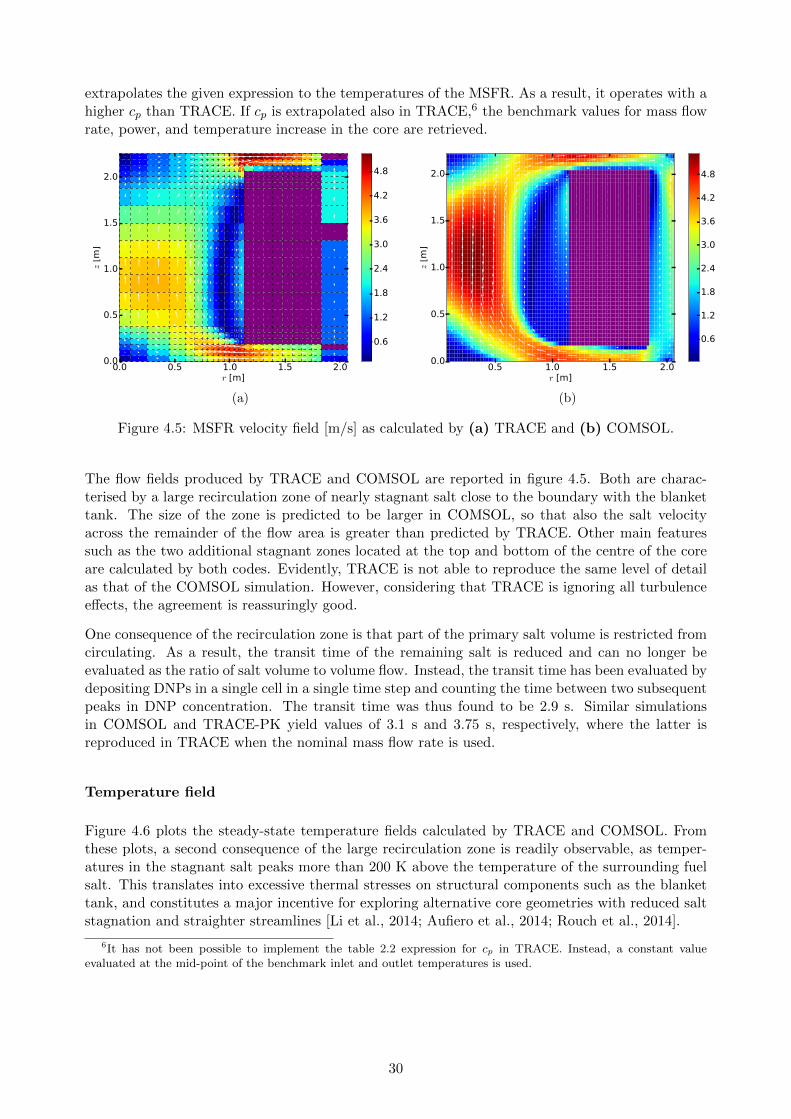
extrapolates the given expression to the temperatures of the MSFR. As a result, it operates with ahigher cp than TRACE. If cp is extrapolated also in TRACE,6 the benchmark values for mass flowrate, power, and temperature increase in the core are retrieved.

0.0 0.5 1.0 1.5 2.0r [m]

0.0

0.5

1.0

1.5

2.0

z [m

]

0.6

1.2

1.8

2.4

3.0

3.6

4.2

4.8

(a)

0.5 1.0 1.5 2.0r [m]

0.0

0.5

1.0

1.5

2.0

z [m

]

0.6

1.2

1.8

2.4

3.0

3.6

4.2

4.8

(b)

Figure 4.5: MSFR velocity field [m/s] as calculated by (a) TRACE and (b) COMSOL.

The flow fields produced by TRACE and COMSOL are reported in figure 4.5. Both are charac-terised by a large recirculation zone of nearly stagnant salt close to the boundary with the blankettank. The size of the zone is predicted to be larger in COMSOL, so that also the salt velocityacross the remainder of the flow area is greater than predicted by TRACE. Other main featuressuch as the two additional stagnant zones located at the top and bottom of the centre of the coreare calculated by both codes. Evidently, TRACE is not able to reproduce the same level of detailas that of the COMSOL simulation. However, considering that TRACE is ignoring all turbulenceeffects, the agreement is reassuringly good.

One consequence of the recirculation zone is that part of the primary salt volume is restricted fromcirculating. As a result, the transit time of the remaining salt is reduced and can no longer beevaluated as the ratio of salt volume to volume flow. Instead, the transit time has been evaluated bydepositing DNPs in a single cell in a single time step and counting the time between two subsequentpeaks in DNP concentration. The transit time was thus found to be 2.9 s. Similar simulationsin COMSOL and TRACE-PK yield values of 3.1 s and 3.75 s, respectively, where the latter isreproduced in TRACE when the nominal mass flow rate is used.

Temperature field

Figure 4.6 plots the steady-state temperature fields calculated by TRACE and COMSOL. Fromthese plots, a second consequence of the large recirculation zone is readily observable, as temper-atures in the stagnant salt peaks more than 200 K above the temperature of the surrounding fuelsalt. This translates into excessive thermal stresses on structural components such as the blankettank, and constitutes a major incentive for exploring alternative core geometries with reduced saltstagnation and straighter streamlines [Li et al., 2014; Aufiero et al., 2014; Rouch et al., 2014].

6It has not been possible to implement the table 2.2 expression for cp in TRACE. Instead, a constant valueevaluated at the mid-point of the benchmark inlet and outlet temperatures is used.

30

0.0 0.5 1.0 1.5 2.0r [m]

0.0

0.5

1.0

1.5

2.0z

[m]

960

1000

1040

1080

1120

1160

1200

(a)

0.5 1.0 1.5 2.0r [m]

0.0

0.5

1.0

1.5

2.0

z [m

]

960

1000

1040

1080

1120

1160

1200

(b)

Figure 4.6: MSFR temperature field [K] as calculated by (a) TRACE and (b) COMSOL.

TRACE is able to reproduce the main trends of the COMSOL temperature solution, with theexception of the hot spot in the bottom, central part of the core which is much more pronouncedin COMSOL. The larger size of the recirculation zone predicted by COMSOL results in a largerhot spot, with a more distributed peak temperature than in TRACE. As a consequence, also theaverage core temperature is higher in COMSOL. It is found to be 1073 K and 1034 K in COMSOLand TRACE, respectively. Also of note is the different temperature distributions in the verticalpart of the recirculation loop. This is because TRACE has the pump above the heat exchanger,while the reverse is true in the COMSOL model.

Pressure field

The pressure distribution calculated by TRACE, reported in figure 4.7, is dominated by the pressurehead generated by the pump, and primarily lost in the heat exchanger. In fact, owing to the elevatedprimary mass flow rate, both the salt velocity inside and pressure loss over the heat exchanger areslightly greater than the reference values given in table 3.2, with magnitudes of 1.25 m/s and 4.35bar. If the mass flow is reduced to near nominal values, the pressure loss over the heat exchanger isapproximately the same as in the COMSOL and TRACE-PK models, where it has been imposed as3 bar at nominal conditions. Contributing factors to the pressure field beyond the pump and heatexchanger are the hydrostatic pressure creating a vaguely discernible gradient from top to bottom,and the expansion vessel, connected to the outermost cell on the top of the reactor model, in whicha pressure of 4.5 bar is imposed in accordance with the TRACE-PK model.

It should be mentioned that actual pressure losses will most surely be higher than the predictionsmade with this model. This is because only frictional losses from wall drag has been taken intoaccount, albeit in abundance in order to emulate viscous shear stresses. Important sources of headloss that have been ignored include abrupt flow area change losses such as those encountered in theheat exchanger, as well as losses in pipe bends, elbows, and the like.

31

0.0 0.5 1.0 1.5 2.0r [m]

0.0

0.5

1.0

1.5

2.0

z [m

]

4.8

5.6

6.4

7.2

8.0

8.8

9.6

10.4

Figure 4.7: MSFR pressure field [bar] as calculated by TRACE.

DNP field

The unconventional behaviour of the DNPs in liquid-fuelled reactors is easily recognisable in figures4.8a-4.8i which display the steady-state spatial concentration of the eight DNP groups and the decayheat deposition. Whereas longer-lived precursors are circulated multiple times and distributed near-uniformly in the primary circuit, the concentration of progressively shorter-lived DNPs approachthe power distribution. In the case of DNP group 8 with a half-life of only 0.2 s, the distributionis nearly the same as the power distribution, only slightly shifted upwards with the flow. Theobtained distributions comply both with intuition and with results from the CFD-based tool fromTU Delft [van der Linden, 2012].

0.0 0.5 1.0 1.5 2.0r [m]

0.0

0.5

1.0

1.5

2.0

z [m

]

0.0e+00

1.0e-04

2.0e-04

3.0e-04

4.0e-04

5.0e-04

6.0e-04

7.0e-04

8.0e-04

9.0e-04

(a) Group 1: T1/2 = 55.6 s.

0.0 0.5 1.0 1.5 2.0r [m]

0.0

0.5

1.0

1.5

2.0

z [m

]

0.0e+00

1.0e-04

2.0e-04

3.0e-04

4.0e-04

5.0e-04

6.0e-04

7.0e-04

8.0e-04

(b) Group 2: T1/2 = 24.5 s.

0.0 0.5 1.0 1.5 2.0r [m]

0.0

0.5

1.0

1.5

2.0

z [m

]

0.0e+00

6.0e-05

1.2e-04

1.8e-04

2.4e-04

3.0e-04

3.6e-04

4.2e-04

4.8e-04

(c) Group 3: T1/2 = 16.3 s.

0.0 0.5 1.0 1.5 2.0r [m]

0.0

0.5

1.0

1.5

2.0

z [m

]

0.0e+00

4.0e-05

8.0e-05

1.2e-04

1.6e-04

2.0e-04

2.4e-04

2.8e-04

(d) Group 4: T1/2 = 5.2 s.

0.0 0.5 1.0 1.5 2.0r [m]

0.0

0.5

1.0

1.5

2.0

z [m

]

0.0e+00

3.0e-05

6.0e-05

9.0e-05

1.2e-04

1.5e-04

1.8e-04

2.1e-04

2.4e-04

(e) Group 5: T1/2 = 2.4 s.

0.0 0.5 1.0 1.5 2.0r [m]

0.0

0.5

1.0

1.5

2.0

z [m

]

0.0e+00

2.5e-06

5.0e-06

7.5e-06

1.0e-05

1.2e-05

1.5e-05

1.7e-05

2.0e-05

(f) Group 6: T1/2 = 1.0 s.

32

0.0 0.5 1.0 1.5 2.0r [m]

0.0

0.5

1.0

1.5

2.0

z [m

]

0.0e+00

2.0e-06

4.0e-06

6.0e-06

8.0e-06

1.0e-05

1.2e-05

1.4e-05

1.6e-05

1.8e-05

(g) Group 7: T1/2 = 0.4 s.

0.0 0.5 1.0 1.5 2.0r [m]

0.0

0.5

1.0

1.5

2.0

z [m

]

0.0e+00

3.0e-07

6.0e-07

9.0e-07

1.2e-06

1.5e-06

1.8e-06

2.1e-06

2.4e-06

(h) Group 8: T1/2 = 0.2 s.

0.0 0.5 1.0 1.5 2.0r [m]

0.0

0.5

1.0

1.5

2.0

z [m

]

0.0e+00

3.0e+05

6.0e+05

9.0e+05

1.2e+06

1.5e+06

1.8e+06

2.1e+06

2.4e+06

(i) Decay heat: T1/2 = 3.2 s.

Figure 4.8: Normalised DNP concentrations for the eight DNP groups and decay heat as calculatedby TRACE. Values in W/m3 for the decay heat, and arbitrary units for the others. Note that theupper limits of the colour legends differ from one plot to another.

An important concept for reactor control is the fraction of delayed neutrons, commonly denotedβ. This concept is extended to the effective delayed neutron fraction, βeff, by taking into accountthe ability of the delayed neutrons to initiate new fission processes. For solid-fuelled reactors, themain source of discrepancy between β and βeff is the energy spectrum of the delayed neutronswhich generally differs from the prompt neutron spectrum. In liquid-fuelled reactors, the positionof precursors in the primary circuit constitute another essential influence. As an example, theneutronic importance of a delayed neutron born inside the heat exchanger is nil.

The effective delayed neutron fraction for DNP group i can be calculated as [Aufiero, 2014; Mattiodaet al., 2000]

βeff,i =

∫φ∗λici∫ ∑

j φ∗λjcj +

∫φ∗νΣfφ

, (4.1)

where φ∗ represents the adjoint flux, j iterates the DNP groups, and the integral is over space andenergy. For the steady-state solution in TRACE, only the power distribution is known. However,for a critical reactor at steady-state, the power deposition correlates well with neutron flux, whichis assumed to sufficiently resemble the adjoint flux for the purposes of this work. Obviously, sinceβeff then depends on recirculation time, power distribution, DNP concentration, core flow field, aswell as fuel composition (affecting β) it represents an excellent figure-of-merit for comparing theability of different codes to calculate liquid-fuel steady-state behaviour. Table 4.5 presents one suchcomparison between TRACE, TRACE-PK, and COMSOL.

Codeβeff,static

[pcm]βeff,moving [pcm]

1 2 3 4 5 6 7 8 Sum [pcm (%)]

TRACE 303.6 7.5 15.4 13.3 21.3 35.4 6.1 11.3 3.3 113.7 (37.4)TRACE-PK 318.1 9.1 17.9 15.6 24.5 40.5 7.1 13.8 3.8 132.1 (41.5)COMSOL 318.1 9.2 18.2 16.2 25.9 42.9 7.4 12.9 3.6 136.3 (42.8)

Table 4.5: βeff in the three different codes. A distinction is made between βeff,static that only takeinto account spectral effects, and βeff,moving that also includes DNP transport. The sum is givenboth in absolute terms, and as a fraction of the static fuel value.

Both TRACE-PK and COMSOL give very similar results since they use the exact same powerdistribution (as determined by COMSOL), and the same value for βeff,static. The value for βeff,static

33

used in TRACE was calculated with Serpent for the fuel composition with a lower fissile contentthan for the other models.

Nevertheless, when the relative size of βeff, moving to βeff, static, hereby referred to as the circulationcorrection factor, cfcirc, is compared, TRACE is still found to produce a lower estimate. Part ofthe reason for this is the elevated mass flow that was required in order to reproduce the core inletand outlet boundary conditions from COMSOL. Indeed, when plotting cfcirc as a function of massflow rate (cf. figure 4.9), it is clearly seen that an increase in mass flow rate is correlated with areduction of delayed neutrons in the core, primarily from the shorter-lived DNP groups. At thenominal mass flow rate of 18500 kg/s, cfcirc ≈ 38.5 %. The remaining discrepancy is likely a resultof the difference in power distributions and the larger recirculation zone in COMSOL that helps toincrease the number of DNP decays that occur in the core.

14 16 18 20 22 24 26 28 30 32Mass flow [103 kg/s]

34

36

38

40

42

44

46

48

cfci

rc [

%]

Total

Group 4

Group 5

Group 6

Figure 4.9: The circulation correction factor for DNP group j, cfcirc,j =βeff, moving,j

βeff, static,j, for selected

groups and the total effective DNP fraction, as a function of the primary mass flow rate.

4.2 Transient behaviour

The strong interdependence between neutronics and thermal-hydraulics exhibited by liquid-fuelledreactors necessitates the use of multi-physics tools for studying time-dependent behaviour. In thiswork, transient analysis of the MSFR has been realised by coupling TRACE with PARCS so thattemperature, DNP, and power deposition fields are exchanged between the two codes. In the coupledtool, PARCS operates with macroscopic cross sections and associated derivatives calculated withSerpent in order to model the strong temperature feedbacks present in the MSFR. To the author’sknowledge, this represents only the second application of the coupled TRACE-PARCS code to anMSR (the first being [Kim, 2015]), and the first in which a multi-dimensional thermal-hydraulicsgeometry is modelled.

On account of the novelty of these simulations, it has been necessary to conduct an assessment ofthe ability of the coupled code to reproduce the dynamic behaviour of the MSFR. To that end, theresults presented in the following have been compared with similar computations performed withthe TRACE-PK and COMSOL tools. It should be noted that since no experimental data existsfor the MSFR also the reference solutions should be approached with a certain level of skepticism.In this way, the objective of this work is code verification rather than validation, that is, to ensurethat the results are in accordance with model expectations.

Prior to simulating dynamic behaviour, a particular procedure for initialising the coupled calcu-lations had to be followed. The specificities of this procedure are detailed in appendix A. In this

34

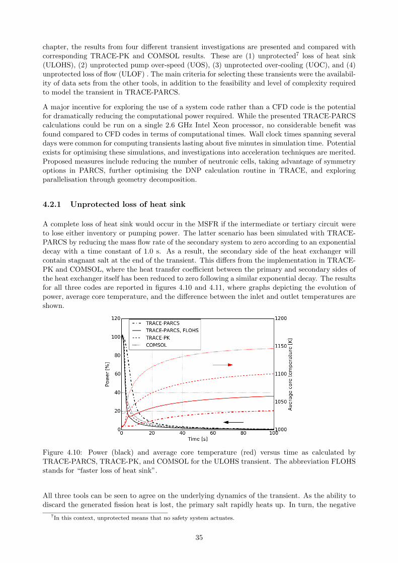
chapter, the results from four different transient investigations are presented and compared withcorresponding TRACE-PK and COMSOL results. These are (1) unprotected7 loss of heat sink(ULOHS), (2) unprotected pump over-speed (UOS), (3) unprotected over-cooling (UOC), and (4)unprotected loss of flow (ULOF) . The main criteria for selecting these transients were the availabil-ity of data sets from the other tools, in addition to the feasibility and level of complexity requiredto model the transient in TRACE-PARCS.

A major incentive for exploring the use of a system code rather than a CFD code is the potentialfor dramatically reducing the computational power required. While the presented TRACE-PARCScalculations could be run on a single 2.6 GHz Intel Xeon processor, no considerable benefit wasfound compared to CFD codes in terms of computational times. Wall clock times spanning severaldays were common for computing transients lasting about five minutes in simulation time. Potentialexists for optimising these simulations, and investigations into acceleration techniques are merited.Proposed measures include reducing the number of neutronic cells, taking advantage of symmetryoptions in PARCS, further optimising the DNP calculation routine in TRACE, and exploringparallelisation through geometry decomposition.

4.2.1 Unprotected loss of heat sink

A complete loss of heat sink would occur in the MSFR if the intermediate or tertiary circuit wereto lose either inventory or pumping power. The latter scenario has been simulated with TRACE-PARCS by reducing the mass flow rate of the secondary system to zero according to an exponentialdecay with a time constant of 1.0 s. As a result, the secondary side of the heat exchanger willcontain stagnant salt at the end of the transient. This differs from the implementation in TRACE-PK and COMSOL, where the heat transfer coefficient between the primary and secondary sides ofthe heat exchanger itself has been reduced to zero following a similar exponential decay. The resultsfor all three codes are reported in figures 4.10 and 4.11, where graphs depicting the evolution ofpower, average core temperature, and the difference between the inlet and outlet temperatures areshown.

Figure 4.10: Power (black) and average core temperature (red) versus time as calculated byTRACE-PARCS, TRACE-PK, and COMSOL for the ULOHS transient. The abbreviation FLOHSstands for “faster loss of heat sink”.

All three tools can be seen to agree on the underlying dynamics of the transient. As the ability todiscard the generated fission heat is lost, the primary salt rapidly heats up. In turn, the negative

7In this context, unprotected means that no safety system actuates.

35

temperature feedback ensures that power levels are greatly reduced. The average core temperaturecan be seen to rise uniformly throughout the transient and gradually reach an asymptotic valueas the fission chain reaction dies down and a uniform temperature distribution is established. Inreality, the primary circuit is not adiabatic outside of the heat exchanger, and heat transfer throughthe vessel walls and to the blanket salt should be considered in future models.

Figure 4.11: ∆T = Tcore,outlet − Tcore,inlet as a function of time as calculated by TRACE-PARCS.TRACE-PK, and COMSOL for the ULOHS transient. The abbreviation FLOHS stands for “fasterloss of heat sink”.

The TRACE-PARCS response is observed to be slower than for the two other tools. This is becausethe primary circuit is able to transfer heat to the intermediate salt for a longer time on account ofthe more realistic heat exchanger modelling. As a way to confirm this, an additional simulation,denoted “faster loss of heat sink”, or FLOHS, has been performed in which the heat exchange isinstantly reduced to zero by equalling the temperature on the secondary side of the heat exchangerwith the temperature on the primary side. Both power and ∆T are then reduced at least as rapidlyas the other predictions.

Interestingly, the oscillatory behaviour of ∆T , seemingly correlated with the transit time, can beseen to disappear in the nominal TRACE-PARCS simulation. This illustrates that the modelling oftemperature distributions along both sides of the heat exchanger has an averaging and smoothingeffect on localised temperature variations such as hot or cold slugs of salt. In comparison, TRACE-PK and COMSOL both rely on constant secondary side temperatures, which hardens the response.Clearly, care must be taken with simplified boundary condition approaches for such strongly coupledsystems. Otherwise, as has been demonstrated, artificial dynamic behaviour can be introduced, orfailed to be captured.

The final average core temperature also varies between the codes. COMSOL predicts the highervalue since the larger recirculation zone stores more thermal energy at the beginning of the transientthan for the three TRACE implementations. The lower value is predicted by the nominal TRACE-PARCS simulation where more energy has been exchanged to the intermediate circuit over thecourse of the transient. Finally, TRACE-PK predicts a higher value than the FLOHS simulationbecause more energy has been deposited in the salt (equal to the integral under the power curves).

36

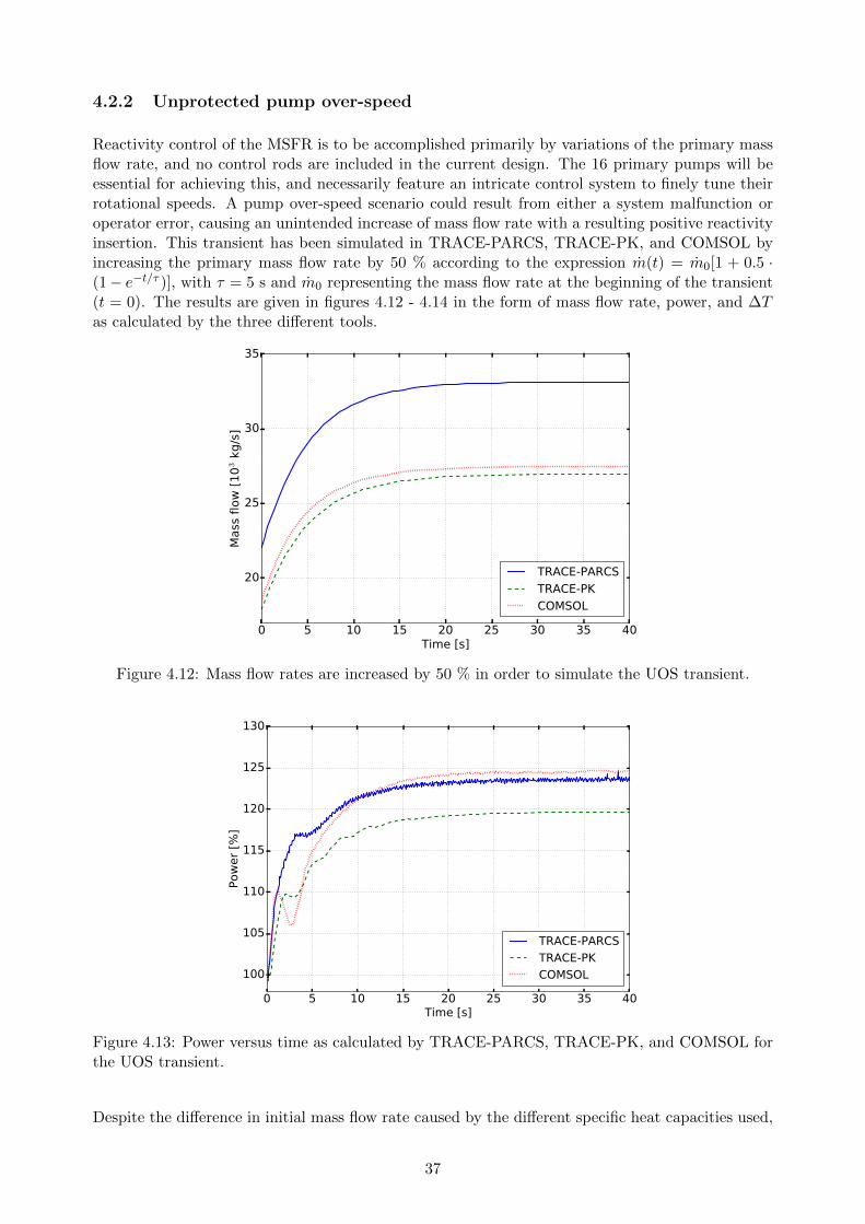
4.2.2 Unprotected pump over-speed

Reactivity control of the MSFR is to be accomplished primarily by variations of the primary massflow rate, and no control rods are included in the current design. The 16 primary pumps will beessential for achieving this, and necessarily feature an intricate control system to finely tune theirrotational speeds. A pump over-speed scenario could result from either a system malfunction oroperator error, causing an unintended increase of mass flow rate with a resulting positive reactivityinsertion. This transient has been simulated in TRACE-PARCS, TRACE-PK, and COMSOL byincreasing the primary mass flow rate by 50 % according to the expression m(t) = m0[1 + 0.5 ·(1− e−t/τ )], with τ = 5 s and m0 representing the mass flow rate at the beginning of the transient(t = 0). The results are given in figures 4.12 - 4.14 in the form of mass flow rate, power, and ∆Tas calculated by the three different tools.

0 5 10 15 20 25 30 35 40Time [s]

20

25

30

35

Mass

flo

w [

10

3 k

g/s

]

TRACE-PARCS

TRACE-PK

COMSOL

Figure 4.12: Mass flow rates are increased by 50 % in order to simulate the UOS transient.

0 5 10 15 20 25 30 35 40Time [s]

100

105

110

115

120

125

130

Pow

er

[%]

TRACE-PARCS

TRACE-PK

COMSOL

Figure 4.13: Power versus time as calculated by TRACE-PARCS, TRACE-PK, and COMSOL forthe UOS transient.

Despite the difference in initial mass flow rate caused by the different specific heat capacities used,

37

the overall transient behaviour predicted by the three codes is again in agreement. As the pumpspeeds up, on one hand βeff decreases, while on the other cold salt reaches further into the corebefore being heated up. The dominant contribution comes from the latter effect, and the positivereactivity introduced is rapidly translated into an increase of power. With the increase in mass flowrate, a smaller enthalpy difference between inlet and outlet is required to carry away the producedpower, and so ∆T decreases. Not shown in the plots are the average core temperatures, which stayalmost constant throughout the transient. Specifically, the variations are -2.9 K, -2.5 K, and +2.3K for TRACE-PARCS, TRACE-PK, and COMSOL, respectively, between the beginning and endof the simulation.

0 5 10 15 20 25 30 35 40Time [s]

80

85

90

95

100

105

110

∆T [

K]

TRACE-PARCS

TRACE-PK

COMSOL

Figure 4.14: ∆T = Tcore,outlet − Tcore,inlet as a function of time as calculated by TRACE-PARCS.TRACE-PK, and COMSOL for the UOS transient.

The main difference between the simulations is ∆T . In TRACE-PARCS the asymptotic valueis below those of TRACE-PK and COMSOL because the mass flow rate is greater, and so theenthalpy increase in the core is smaller. Since also the magnitude of the mass flow rate increase isgreater in the TRACE-PARCS simulation, the difference between ∆T from COMSOL and TRACE-PARCS has increased at the end of the simulation. The TRACE-PK simulation differs in that theasymptotic power level is lower than for the two other codes. According to [Zanetti, 2016], thisdiscrepancy is suspected to be caused by the variations of the βeff incurred by the mass flow rateincrease. Lastly, power and ∆T fluctuations related to the simplified heat exchanger implementationin COMSOL and TRACE-PK are again suppressed in the TRACE-PARCS simulation.

4.2.3 Unprotected over-cooling

Regardless of the choice of working fluid in the tertiary turbine circuit of an MSFR plant, be itwater or super critical CO2, it will have to be pressurised. Thus, a possibility will exist for thetertiary circuit to be inadvertently depressurised releasing large quantities of thermal energy in anuncontrolled fashion. This will, in turn, extract excessive amounts of heat from the intermediatecircuit, which will cool the primary circuit. Such over-cooling transient can be simulated by reducingthe inlet temperature on the secondary side of the primary heat exchanger by 100 K according toan exponential decay with a time constant of 1 s. This has been performed in TRACE-PARCS,while in TRACE-PK and COMSOL the imposed temperature on the secondary side of the heatexchanger was lowered similarly. The results are presented in figures 4.15 - 4.17.

38

0 10 20 30 40 50Time [s]

800

850

900

950

1000

1050

Tem

pera

ture

[K

]

TRACE-PARCS, 70 K

TRACE-PARCS, 100 K

TRACE-PK

COMSOL

Figure 4.15: Inlet (blue, bottom) and outlet temperatures (red, top) as a function of time ascalculated by TRACE-PARCS, TRACE-PK, and COMSOL for the UOC transient. 70 K denotesan additional simulation in which the temperature at the inlet of the heat exchanger was loweredby 70 K instead of 100 K.

Like the UOS transient, the evolution of the UOC transient is driven by the introduction of cold saltinto the reactor core as the core inlet temperature is decreased. In response, the neutronic powerincreases until a new equilibrium between heat generation and removal is established. In figure 4.16,both TRACE codes show the initial decrease in average core temperature (albeit damped in theTRACE-PARCS simulations because of the more realistic heat exchanger), followed by an increaseuntil the reactor stabilises at the new equilibrium power level. For COMSOL, the core temperatureevolution is decreasing. Thus, it appears as if the decreased inlet temperature interferes with andreduces the size of the hot recirculation zone. This dynamic behaviour is not reproduced by eitherTRACE code.

0 10 20 30 40 50Time [s]

20

40

60

80

100

120

140

160

180

200

Pow

er

[%]

TRACE-PARCS, 100 K

TRACE-PARCS, 70 K

TRACE-PK

COMSOL990

1000

1010

1020

1030

1040

1050

Avera

ge c

ore

tem

pera

ture

[K

]

Figure 4.16: Power (black) and average core temperature (red) versus time as calculated byTRACE-PARCS, TRACE-PK, and COMSOL for the UOC transient. 70 K denotes an additionalsimulation in which the temperature at the inlet of the heat exchanger was lowered by 70 K insteadof 100 K.

As can be seen in figure 4.15, the decrease in core inlet temperature is greater in the TRACE-PARCS simulation than for the two other codes. In fact, an inlet temperature of 850 K is only

39

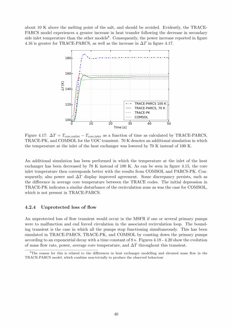
about 10 K above the melting point of the salt, and should be avoided. Evidently, the TRACE-PARCS model experiences a greater increase in heat transfer following the decrease in secondaryside inlet temperature than the other models8. Consequently, the power increase reported in figure4.16 is greater for TRACE-PARCS, as well as the increase in ∆T in figure 4.17.

0 10 20 30 40 50Time [s]

100

120

140

160

180∆T [

K]

TRACE-PARCS 100 K

TRACE-PARCS, 70 K

TRACE-PK

COMSOL

Figure 4.17: ∆T = Tcore,outlet − Tcore,inlet as a function of time as calculated by TRACE-PARCS,TRACE-PK, and COMSOL for the UOC transient. 70 K denotes an additional simulation in whichthe temperature at the inlet of the heat exchanger was lowered by 70 K instead of 100 K.

An additional simulation has been performed in which the temperature at the inlet of the heatexchanger has been decreased by 70 K instead of 100 K. As can be seen in figure 4.15, the coreinlet temperature then corresponds better with the results from COMSOL and PARCS-PK. Con-sequently, also power and ∆T display improved agreement. Some discrepancy persists, such asthe difference in average core temperature between the TRACE codes. The initial depression inTRACE-PK indicates a similar disturbance of the recirculation zone as was the case for COMSOL,which is not present in TRACE-PARCS.

4.2.4 Unprotected loss of flow

An unprotected loss of flow transient would occur in the MSFR if one or several primary pumpswere to malfunction and end forced circulation in the associated recirculation loop. The bound-ing transient is the case in which all the pumps stop functioning simultaneously. This has beensimulated in TRACE-PARCS, TRACE-PK, and COMSOL by coasting down the primary pumpsaccording to an exponential decay with a time constant of 8 s. Figures 4.18 - 4.20 show the evolutionof mass flow rate, power, average core temperature, and ∆T throughout this transient.

8The reason for this is related to the differences in heat exchanger modelling and elevated mass flow in theTRACE-PARCS model, which combine non-trivially to produce the observed behaviour

40

0 10 20 30 40 50Time [s]

0

5

10

15

20

25

Mass

flo

w [

10

3 k

g/s

]

TRACE-PARCS

TRACE-PK

COMSOL

Figure 4.18: Mass flow rate as a function of time as calculated by TRACE-PARCS, TRACE-PK,and COMSOL for the ULOF transient. While natural circulation is established in the COMSOLand TRACE-PK simulations, TRACE-PARCS predicts almost stagnation of the fuel salt.

0 50 100 150 200 250 300 350Time [s]

0

20

40

60

80

100

120

Pow

er

[%]

TRACE-PARCS

TRACE-PK

COMSOL

980

990

1000

1010

1020

1030

1040

1050

1060

1070

Avera

ge c

ore

tem

pera

ture

[K

]

Figure 4.19: Power (black) and average core temperature (red) as a function of time as calcu-lated by TRACE-PARCS, TRACE-PK, and COMSOL for the ULOF transient. The average coretemperature evolution for the COMSOL simulation was only calculated until 200 s.

0 50 100 150 200 250 300 350Time [s]

0

50

100

150

200

250

300

350

400

∆T [

K]

TRACE-PARCS

TRACE-PK

COMSOL

Figure 4.20: ∆T = Tcore,outlet − Tcore,inlet as a function of time as calculated by TRACE-PARCS,TRACE-PK, and COMSOL for the ULOF transient.

For this transient, the three codes do not agree on the general dynamics. Whereas natural circula-

41

tion is established in TRACE-PK and COMSOL, TRACE-PARCS predicts near-stagnation of thefuel salt. As a consequence, the reactor experiences both degraded heat removal and an increasedβeff that work together to increase the temperature until the neutron chain reaction is effectivelystopped by temperature feedbacks. However, since the secondary side continues to extract heat,the average core temperature begins to decline. Furthermore, in the now nearly stagnant core, hotsalt floats to the top and cold salt sinks to the bottom, creating a large temperature gradient thatmaintains a high ∆T . As more thermal energy is extracted in the heat exchanger, the cold region atthe bottom creeps upwards and the core gradually approaches a uniform temperature distribution.

The absence of natural circulation in TRACE-PARCS is a result of having the heat exchangerplaced below the pump. Placing the heat sink, i.e., the heat exchanger, at an elevated positioncompared to the heat source, i.e., the core, benefits natural circulation, and has been done in thetwo other models. As a result, TRACE-PK and COMSOL calculate a mass flow rate about tentime greater than TRACE-PARCS at the new equilibrium conditions. In an attempt to improvethe comparison, TRACE-PARCS simulations have been performed with the heat exchanger on topof the pump. However, as the length of the heat exchanger made it impossible to place it as highas in the other models, only modest improvements were observed and considerate discrepanciespersisted.

Evidently, also TRACE-PK and COMSOL compute quite different solutions. In fact, in a com-parison between COMSOL and another CFD-based tool from TU Delft, significant discrepanciesbetween the computed behaviours in the ULOF transient are also reported [Fiorina, 2013]. Thisindicates that this transient is particularly sensitive to the modelling of components such as heatexchangers, pumps, as well as treatment of friction. Adding to the complexity, natural circula-tion of fluids with internal heat generation from the distributed decay heat constitutes a largelyunexplored field that is currently under investigation [Cammi et al., 2016].

Finally, it is noted that current plans for decay heat removal (DHR) relies on dumping the saltto the dump tanks where the heat can be more easily removed. Despite this, several incentivesfor studying the natural circulation phenomenon exist. First, an increased reliance on naturalcirculation for DHR could improve plant economics by avoiding the draining, freezing and eventualthawing and reintroduction of the salt from the drain tanks. Second, natural circulation wouldhave to be relied on in case of malfunction in the drainage system. Third, considerable time mightpass while the salt is in the process of draining. Natural circulation would provide additional heatremoval during this time interval.

42

5 Conclusions and outlook

This thesis has reported the application of the coupled TRACE-PARCS multi-physics code totransient analyses of the MSFR. The main goal has been to assess the ability of this tool to predictdynamic behaviour of the MSFR through comparison with alternative code systems. A secondarygoal has been to display and characterise distinguishing features of MSRs based on the steady-stateand transient simulations performed.

In order to assemble the coupled tool, a simplified, axially-symmetric benchmark model of theMSFR was separately implemented in the codes TRACE, PARCS, and Serpent. The purpose ofthe Serpent model was to generate spatially homogenised, multi-group, macroscopic cross sectionsthat allowed PARCS to capture the strong temperature feedback effects exhibited by the MSFR. Toadvise the modelling of the breeding blanket, Monte Carlo simulations were performed with MCNPto investigate power deposition during steady-state. The blanket was found to have negligibleinfluence on the primary circuit, and was thus neglected in the TRACE and PARCS models.However, under transient conditions a stronger influence is likely and warrants further investigation.

Steady-state simulations were performed with the three codes in order to initialise transient calcu-lations and to explore the MSFR phenomenology. Neutron flux distribution and spectrum, temper-ature feedback coefficients, primary circuit temperature, pressure, velocity, and DNP distributions,the effective delayed neutron fraction, and transit time have been investigated and discussed.

Comparisons of the thermal-hydraulic steady-state solution were made with a CFD solver basedon COMSOL. Although TRACE proved unable to reproduce the level of detail of COMSOL,main features were found to be consistent after calibration against the COMSOL solution. Animportant source of discrepancy was the difference in specific heat capacity values used in the twocodes. TRACE used a lower value, and thus required a higher mass flow rate to maintain thesame temperature rise over the core. Similarly, the neutronic steady-state solution calculated byPARCS was found to correlate well with Serpent after an initial calibration of the albedo condition.Discrepancies on the order of 1-2 % in temperature coefficients are reported. The need for higher-accuracy solutions to calibrate the steady-state models should be emphasised, as this requirementwill also apply to the coupled tool.

Four transients were simulated with TRACE-PARCS and compared with solutions from the CFD-tool COMSOL (coupled with a spatial diffusion solver) and TRACE-PK (TRACE together witha simplified point kinetics routine). The three tools were found to generally agree on transientdynamics. However, direct comparison was often complicated due to differences in modelling. Forinstance, the heat exchangers were implemented in a more realistic manner in TRACE-PARCS.Where more direct comparisons were facilitated, reasonable agreement was found. As such, theobserved discrepancies are in large parts due to differences in modelling. Of the discrepancies thatcould not be traced to modelling choices (e.g. the evolution of average core temperature), manyare related to differences in the underlying equations solved by the codes and the resolution of thecomputational meshes. Based on these observations and insights, it is concluded that the TRACE-PARCS coupled tool, to a reasonable extent, is able to reproduce the main features of dynamicMSFR behaviour as predicted by the other multi-physics tools.

43

A particularly interesting discrepancy between TRACE-PARCS and the two other tools was theexistence of power and temperature oscillations with characteristic times similar to the transit time.While COMSOL and TRACE-PK predicted such fluctuations in the UOS and ULOHS transients,TRACE-PARCS showed a much smoother behaviour. It has been shown that this behaviouraldifference stems from the explicit modelling of a secondary circuit in TRACE-PARCS, whereasCOMSOL and TRACE-PK impose a constant secondary side temperature. This highlights theimportance of imposed boundary conditions on strongly coupled systems such as the MSFR.

In general, TRACE-PARCS seems to agree well with TRACE-PK. This indicates that spatialkinetics are not required to model the transients investigated herein, but that point kinetics aresufficient. Since point kinetics calculations are also faster to execute, they represent the superioralternative when little to no asymmetry is expected. Conversely, for asymmetric transients such assingle pump failure, spatial kinetics tools are expected to yield more accurate solutions.

One notable exception to the general agreement between the three tools was the ULOF transient.It exhibits strong dependence on modelling choices related to pumps, heat exchangers, as wellas treatment of friction, which makes it particularly complicated to simulate. Furthermore, itconsiders natural circulation of internally heated fluids, for which systematic investigation has onlyrecently begun [Cammi et al., 2016].

Ultimately, TRACE-PARCS has been found to represent a viable tool for calculating transientbehaviour of the MSFR when computational resources are scarce or the considered model is large.That being said, while only a single processor was used to run transients on, computational timeswere prohibitively long, commonly several days. Attempts at optimising the MSFR model imple-mentations as well as the TRACE-PARCS tool are therefore merited. The availability of built-incomponent models in TRACE facilitated realistic modelling of heat exchangers and pumps, whilethe comprehensive control logic system simplified the simulation of transients. In sum, TRACE-PARCS represents a flexible and powerful multi-physics code that can be easily extended to inves-tigate additional transients and more extensive MSFR plant systems.

Continued research into TRACE-PARCS and related topics could progress in a number of differentdirections. First and foremost, efforts should be made at improving the computational efficiency toaccelerate calculations. Suggestions include model order reduction, employing symmetry optionsin PARCS, further optimising the DNP solution routine in TRACE, and enabling parallelisationthrough domain decomposition. With improved run times, an extension to full three-dimensionalmodels is straightforward and would permit investigation of asymmetric transients so as to furtherassess the influence of the spatial kinetics solution.

Only the primary and a simplified secondary circuit were considered in this project. However, asTRACE is equipped with two-phase flow equations, the modelling of entire MSFR plants includ-ing turbine circuits with liquid water and steam is readily attainable. Moreover, two-phase fluidcapabilities can be used to model gas bubbles in the molten salt. Thus, the effects of fission gasformation and tritium bubble inclusion in the primary salt can be studied, or the helium bubblingtechnique that has been proposed to extract fission products from the MSFR [Journee, 2014].

Lastly, an additional area to explore is the coupling of a system code such as TRACE with a high-accuracy CFD code. In such an arrangement, thermal-hydraulic behaviour within and out-of-corewould be calculated by the CFD and system code, respectively. Explicit coupling is accomplishedby data transfer at the boundaries between the two models. Thus, computational requirements arekept manageable by only invoking the CFD solver in a restricted region of space. Furthermore,for the specific case of TRACE, such symbiosis would overcome the restriction of rectangular orcylindrical core shapes that currently limit the applicability of TRACE to more recent MSFR designiterations. Some investigations into this area exist [Bertolotto, 2011; Zanetti, 2016], although moreremain to be learned.

44

Bibliography

[Ariu, 2014] Ariu, V. (2014). Heat exchanger analysis for innovative molten salt fast reactor. Master’s thesis,Eidgenossische Technische Hochschule Zurich (ETHZ) and Ecole polytechnique federale de Lausanne (EPFL).

[Aufiero, 2014] Aufiero, M. (2014). Development of advanced simulation tools for circulating-fuel nuclear reactors.PhD thesis, Politecni di Milano, Department of Energy.

[Aufiero et al., 2014] Aufiero, M., Cammi, A., Geoffroy, O., Losa, M., Luzzi, L., Ricotti, M. E., and Rouch, H. (2014).Development of an OpenFOAM model for the Molten Salt Fast Reactor transient analysis. Chemical EngineeringScience, 111:390–401.

[Auger et al., 2008] Auger, T., Barreau, G., Chevalier, J.-P., Doligez, X., Delpech, S., Flocard, H., Haas, B., Heuer,D., and Merle-Lucotte, E. (2008). The CNRS Research Program on the Thorium cycle and the Molten SaltReactors. Technical report, Centre National de la Recherche Scientifique.

[Benes and Konigs, 2012a] Benes, O. and Konigs, R. J. M. (2012a). Molten Salt Reactor Fuel and Coolant. InKonigs, R. J. M., editor, Comprehensive Nuclear Materials, chapter 3.13. Elsevier Ltd.

[Benes and Konigs, 2012b] Benes, O. and Konigs, R. J. M. (2012b). Thermodynamic Calculations of Molten-SaltReactor Fuel Systems. In Konigs, R. J. M., editor, Comprehensive Nuclear Materials, chapter 4. Elsevier Ltd.

[Bertolotto, 2011] Bertolotto, D. (2011). Coupling a System Code with Computational Fluid Dynamics for the Sim-ulation of Complex Coolant Reactivity Effects. PhD thesis, Ecole polytechnique federale de Lausanne (EPFL).

[Brovchenko, 2013] Brovchenko, M. (2013). Etudes preliminaires de surete du reacteur a sels fondus MSFR. PhDthesis, Laboratoire de Physique Subatomique et de Cosmologie de Grenoble, Universite Grenoble Alpes.

[Cammi et al., 2016] Cammi, A., Cauzzi, M., Luzzi, L., and Pini, A. (2016). Dynasty: an experimental loop for thestudy of natural circulation with internally heated fluids. In Conference: 12th International Conference on HeatTransfer, Fluid Mechanics and Thermodynamics (HEFAT 2016), Malaga, Spain.

[Chadwick et al., 2011] Chadwick, M. B., Herman, M., Oblozinsky, P., Dunn, M. E., Danon, Y., Kahler, A. C.,Smith, D. L., Pritychenko, B., Arbanas, G., Arcilla, R., Brewer, R., Brown, D. A., Capote, R., Carlson, A. D.,Cho, Y. S., Derrien, H., Guber, K., Hale, G. M., Hoblit, S., Holloway, S., Johnson, T. D., Kawano, T., Kiedrowski,B. C., Kim, H., Kunieda, S., Larson, N. M., Leal, L., Lestone, J. P., Little, R. C., McCutchan, E. A., MacFarlane,R. E., MacInnes, M., Mattoon, C. M., McKnight, R. D., Mughabghab, S. F., Nobre, G. P. A., Palmiotti, G.,Palumbo, A., Pigni, M. T., Pronyaev, V. G., Sayer, R. O., Sonzogni, A. A., Summers, N. C., Talou, P., Thompson,I. J., Trkov, A., Vogt, R. L., van der Marck, S. C., Wallner, A., White, M. C., Wiarda, D., and Young, P. G.(2011). ENDF/B-VII.1 nuclear data for science and technology: Cross sections, covariances, fission product yieldsand decay data.

[Cherubini et al., 2011] Cherubini, F., Peters, G., Berntsen, T., Strømman, A. H., and Hertwich, E. (2011). CO2emissions from biomass combustion for bioenergy: atmospheric decay and contribution to global warming. GBCBioenergy, 3.

[CNSC, 2015] CNSC (2015). Update on Regulatory Vendor Design Review of Advanced Reactor Designs in Canada.Presentation to the IAEA by R. P. Rulko.

[COMSOL, 2012] COMSOL (2012). COMSOL Multiphysics User’s Guide. COMSOL, Inc., version 4.3a.

[Doligez, 2010] Doligez, X. (2010). Influence du retraitement physico-chimique du sel combustible sur le comportementdu MSFR et sur le dimensionnement de son unite de retraitement. PhD thesis, Institut National Polytechniquede Grenoble (INPG).

[Downar et al., 2009] Downar, T., Xu, Y., and Seker, V. (2009). Purdue Advanced Reactor Core Simulator (PARCS)v.3 Theory Manual.

[Fiorina, 2013] Fiorina, C. (2013). The Molten Salt Fast Reactor as a Fast-Spectrum Candidate for Thorium Imple-mentation. PhD thesis, Politecnico di Milano, Department of Energy.

[Fiorina et al., 2013] Fiorina, C., Aufiero, M., Cammi, A., Franceschini, F., Krepel, J., Luzzi, L., Mikityuk, K., andRicotti, M. E. (2013). Investigation of the MSFR core physics and fuel cycle options. Progress in Nuclear Energy,68.

45

[Forsberg et al., 2003] Forsberg, C. W., Peterson, P. F., and Pickard, P. S. (2003). Molten-Salt-Cooled AdvancedHigh-Temperature Reactor for Production of Hydrogen and Electricity. ANS Nuclear Technology, 144:289–302.

[Ghasabyan, 2013] Ghasabyan, L. K. (2013). Use of Serpent Monte-Carlo code for development of 3D full-core modelsof Gen-IV fast-spectrum reactors and preparation of group constants for transient analyses with PARCS/TRACEcoupled system. Master’s thesis, Royal Institute of Technology, KTH.

[GIF, 2002] GIF (2002). A Technology Roadmap for Generation IV Nuclear Energy Systems. Issued by the U.S.DOE Nuclear Energy Research Advisory Committee and the Generation IV International Forum.

[Haubenreich and Engel, 1970] Haubenreich, P. N. and Engel, J. R. (1970). Experience with the Molten-Salt ReactorExperiment. Nuclear applications and technology, 8.

[Haynes International, 2015] Haynes International (2015). HASTELLOY R©N alloy. Product brochure available fromhaynesintl.com [PDF].

[IEA, 2015a] IEA (2015a). Key World Energy Statistics.

[IEA, 2015b] IEA (2015b). World Energy Outlook. OECD/IEA. ISBN: 978-92-64-24365-1.

[Johnson, 2009] Johnson, E. (2009). Goodbye to carbon neutral: Getting biomass footprints right. EnvironmentalImpact Assessment Review, 29.

[Journee, 2014] Journee, D. (2014). Helium bubbling in a Molten Salt Fast Reactor. Master’s thesis, Delft Universityof Technology, Faculty of Applied Physics.

[Kakodkar and Degweker, 2013] Kakodkar, A. and Degweker, S. B. (2013). Towards Sustainable, Secure, and SafeEnergy Future: Leveraging Opportunities with Thorium. In Proceedings of the ThEC13 Conference, Geneva,Switzerland.

[Kedl, 1972] Kedl, R. J. (1972). The migration of a class of fission products (noble metals) in the molten-salt reactorexperiment. Technical report, ORNL. ORNL-TM-3884.

[Kim, 2015] Kim, H.-M. (2015). Static and transient analysis of Molten Salt Reactor Experiment using SERPENT-2/TRACE/PARCS codes. Master’s thesis, Eidgenossische Technische Hochschule Zurich (ETHZ) and Ecole poly-technique federale de Lausanne (EPFL).

[Leppanen, 2013] Leppanen, J. (2013). Serpent - a Continuous-energy Monte Carlo Reacter Physics Burnup Cal-culation Code, User’s Manual. VTT Technical Research Centre of Finland. Note: Serpent-2.1.26 has been usedthroughout this work.

[Leppanen et al., 2014] Leppanen, J., Aufiero, M., Fridman, E., Rachamin, R., and van der Marck, S. (2014). Cal-culation of effective point kinetics parameters in the Serpent 2 Monte Carlo code. Annals of Nuclear Energy,65:272–279.

[Li et al., 2014] Li, R., Wang, S., Rineiski, A., Zhang, D., and Merle-Lucotte, E. (2014). Transient analyses for amolten salt fast reactor with optimized core geometry. Nuclear Engineering and Design.

[MacPherson, 1985] MacPherson, H. G. (1985). The Molten Salt Reactor Adventure. Nucler Science and Engineering,90.

[Mathers and Hesketh, 2013] Mathers, D. and Hesketh, K. (2013). A View on the Thorium Fuel Cycle. In Proceedingsof the ThEC13 Conference, Geneva, Switzerland.

[Mathieu et al., 2006] Mathieu, L., Heuer, D., Brissot, R., Brun, C. L., Liatard, E., Loiseaux, J.-M., Meplan, O.,Merle-Lucotte, E., Nuttin, A., and Wilson, J. (2006). The Thorium Molten Salt Reactor: Moving On from theMSBR. Progress in Nuclear Energy, 48.

[Mattioda et al., 2000] Mattioda, F., Ravetto, P., and Ritter, G. (2000). Effective delayed neutron fraction forfluid-fuel systems. Annals of Nuclear Energy, 27:1523–1532.

[Merle-Lucotte et al., 2011] Merle-Lucotte, E., Heuer, D., Allibert, M., Brovchenko, M., Capellan, N., and Ghetta, V.(2011). Launching the Thorium Fuel Cycle with the Molten Salt Fast Reactor. In Proceedings of the InternationalCongress on Advances in Nuclear Power Plants (ICAPP) 2011, Nice, France.

[Merle-Lucotte et al., 2008] Merle-Lucotte, E., Heuer, D., Allibert, M., Doligez, X., Ghetta, V., and Brun, C. L.(2008). Optimization and simplification of the concept of non-moderated Thorium Molten Salt Reactor. InProceedings of the International Conference on the Physics of Reactors (PHYSOR) 2008, Interlaken, Switzerland.

[Mikityuk et al., 2005] Mikityuk, K., Pelloni, S., Coddington, P., Bubelis, E., and Chawla, R. (2005). FAST: Anadvanced code system for fast reactor transient analysis. Annals of Nuclear Energy, 32.

[Nagy et al., 2010] Nagy, K., Kloosterman, J. L., Lathouwers, D., and van der Hagen, T. H. J. J. (2010). Newbreeding gain definitions and their application to the optimization of a molten salt reactor design. Annals ofNuclear Energy, 38.

[NEA, 2015] NEA, O. (2015). Introduction of Thorium in the Nuclear Fuel Cycle - Short- to long-term considerations. NEA no. 7228.

[NRC, 2007] NRC (2007). TRACE v.5 User’s Manual.

46

[NRC, 2012] NRC (2012). Report to Congress: Advanced Reactor Licensing.

[Patankar, 1980] Patankar, S. V. (1980). Numerical Heat Transfer and Fluid Flow. Hemisphere Publishing Corpo-ration.

[Pelowitz et al., 2014] Pelowitz, D. B., Fallgren, A. J., and (Eds.), G. E. M. (2014). MCNP6 User’s Manual.

[Penny, 2010] Penny, S. L. (2010). A Study of the Advantages of Thorium Reactors for Nuclear Power. Master’sthesis, Faculty of Engineering and Physical Sciences, University of Surrey.

[Pioro, 2016] Pioro, I., editor (2016). Handbook of Generation IV Nuclear Reactors. Woodhead Publishing. ISBN:9780081001493.

[Pope and Mousseau, 2009] Pope, M. A. and Mousseau, V. A. (2009). Accuracy and efficiency of a coupled neutronicsand thermal hydraulics model. Nuclear Engineering and Technology, 41.

[Rangel and Leveque, 2015] Rangel, L. E. and Leveque, F. (2015). Revisiting the Cost Escalation Curse of NuclearPower: New Lessons from the French Experience. Economics of Energy & Environmental Policy, 4.

[Rimpault et al., 2002] Rimpault, G., Plisson, D., Tommasi, J., Jacqmin, R., Rieunier, J.-M., Verrier, D., and Biron,D. (2002). The ERANOS code and data system for fast reactor neutronic analyses. In Proceedings of the Interna-tional Conference on the Physics of Reactors (PHYSOR), Seoul, Korea.

[Rosenthal, 2009] Rosenthal, M. W. (2009). An Account of Oak Ridge National Laboratory’s Thirteen NuclearReactors. ORNL/TM-2009/181.

[Rouch et al., 2014] Rouch, H., Geoffroy, O., Rubiolo, P., Laureau, A., Brovchenko, M., Merle-Lucotte, E., andHeuer, D. (2014). Preliminary Thermal-hydraulic Core Design of the Molten Salt Fast Reactor (MSFR). Annalsof Nuclear Energy.

[Sabharwall et al., 2011] Sabharwall, P., Kim, E. S., McKellar, M., and Anderson, N. (2011). Process Heat ExchangerOptions for Fluoride Salt High Temperature Reactor. Technical report, Idaho National Laboratory. Prepared forthe U.S. Department of Energy.

[Samuel, 2009] Samuel, D. (2009). Molten salt coolants for high temperature reactors - a literature summary ofkey R&D activities and challenges. Technical report, IAEA INPRO. Internship report for the INPRO COOLcollaborative project.

[Santamarina et al., 2009] Santamarina, A., Bernard, D., Blaise, P., Coste, M., Courcelle, A., Huynh, T., Jouanne,C., Leconte, P., Litaize, O., Mengelle, S., Noguere, G., Ruggieri, J.-M., Serot, O., Tommasi, J., Vaglio, C., andVidal, J.-F. (2009). The JEFF-3.1.1 Nuclear Data Library. Technical report, OECD NEA. ISBN 978-92-64-99074-6.

[Serp et al., 2014] Serp, J., Allibert, M., Benes, O., Delpech, S., Feynberg, O., Ghetta, V., Heuer, D., Holcomb, D.,Ignatiev, V., Kloosterman, J. L., Luzzi, L., Merle-Lucotte, E., Uhlır, J., Yoshioka, R., and Zhimin, D. (2014). Themolten salt reactor (MSR) in generation IV: Overview and perspectives. Progress in Nuclear Energy, 77.

[Sokolov et al., 2005] Sokolov, F., Fukuda, K., and Nawada, H. P. (2005). Thorium fuel cycle — Potential benefitsand challenges. Technical report, IAEA.

[van der Linden, 2012] van der Linden, E. (2012). Coupled neutronics and computational fluid dynamics for themolten salt fast reactor. Master’s thesis, Delft University of Technology, Faculty of Applied Physics.

[Waltar et al., 2012] Waltar, A. W., Todd, D. R., and Tsvetkov, P. V. (2012). Fast Spectrum Reactors. SpringerScience+Business Media, LLC. ISBN 978-1-4419-9571-1.

[X-5 Monte Carlo Team, 2003] X-5 Monte Carlo Team (2003). MCNP - A General Monte Carlo N-Particle TransportCode, Version 5. Volume I: Overview and Theory. LA-UR-03-1987, Los Alamos National Laboratory, Los Alamos,N.M.

[Zanetti, 2016] Zanetti, M. (2016). Development of new tools for the analysis and simulation of circulating-fuelreactor power plants. PhD thesis, Politecni di Milano, Department of Energy.

[Zanetti et al., 2015] Zanetti, M., Cammi, A., Luzzi, L., Krepel, J., and Mikityuk, K. (2015). Extension of the FASTcode system for the modelling and simulation of MSR dynamics. In ICAPP 2015: Proceedings of the InternationalCongress on Advances in Nuclear Power Plants.

47

List of abbreviations

ARE Aircraft Reactor Experiment

AU arbitrary units

CFD computational fluid dynamics

CMFD coarse mesh finite difference

DHR decay heat removal

DNP delayed neutron precursor

EVOL Evaluation and Viability Of Liquid fuel fast reactor system

FLiBe LiF-BeF2

GIF Generation IV International Forum

IEA International Energy Agency

LWR light water reactor

MSR molten salt reactor

MSFR Molten Salt Fast Reactor

MSBR Molten Salt Breeder Reactor

MSRE Molten Salt Reactor Experiment

NEA Nuclear Energy Agency

NRC US Nuclear Regulatory Commission

ORNL Oak Ridge National Laboratory

PARCS Purdue Advanced Reactor Core Simulator

pcm per cent mille

PSI Paul Scherrer Institut

PK point kinetics

TRACE TRAC/RELAP Advanced Computational Engine

TRACE-PK the TRACE code extended with DNP and point kinetics capabilities

TU Delft Delft University of Technology

ULOF unprotected loss of flow

ULOHS unprotected loss of heat sink

UOC unprotected over-cooling

UOS unprotected pump over-speed

VVER Vodo-Vodyanoi Energetichesky Reaktor (in English: Water-Water Power Reactor)

48

Nomenclature

Latin symbols Greek symbols

a albedo value

cj concentration of DNP group j

Cw wall drag coefficient

cfcirc circulation correction factor

Dm molecular diffusivity

Dn neutron diffusion coefficient

e specific internal energy

fw wall friction force (per volume)

g gravitational constant

J neutron current

k turbulent kinetic energy

keff neutron multiplication factor

kwChurchill correlation frictionfactor

m mass flow rate

n neutron density

p pressure

qf direct fluid heating

qw wall heating

Re Reynolds number

t time

T temperature

T1/2 half-life

u fluid velocity

v neutron velocity

αD Doppler reactivity coefficient

αToverall temperature reactivitycoefficient

αρfuel salt density reactivitycoefficient

βeffeffective delayed neutronfraction

βjdelayed neutron fraction forDNP group j

χd DNP decay neutron yield

χp fission neutron yield

δ surface roughness

∆TCore inlet and outlettemperature difference

ε turbulent dissipation

νaverage number of neutrons perfission

φ neutron flux

φ∗ adjoint neutron flux

λ decay constant

ρ density

Σ macroscopic cross section

Boldface indicates vector quantities.

49

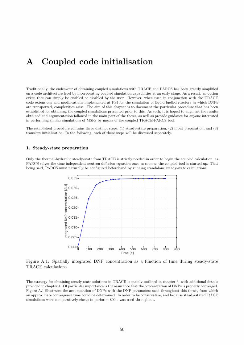
A Coupled code initialisation

Traditionally, the endeavour of obtaining coupled simulations with TRACE and PARCS has been greatly simplifiedon a code architecture level by incorporating coupled simulation capabilities at an early stage. As a result, an optionexists that can simply be enabled or disabled by the user. However, when used in conjunction with the TRACEcode extensions and modifications implemented at PSI for the simulation of liquid-fuelled reactors in which DNPsare transported, complexities arise. The aim of this chapter is to document the particular procedure that has beenestablished for obtaining the coupled simulations presented prior to this. As such, it is hoped to augment the resultsobtained and argumentation followed in the main part of the thesis, as well as provide guidance for anyone interestedin performing similar simulations of MSRs by means of the coupled TRACE-PARCS tool.

The established procedure contains three distinct steps; (1) steady-state preparation, (2) input preparation, and (3)transient initialisation. In the following, each of these steps will be discussed separately.

1. Steady-state preparation

Only the thermal-hydraulic steady-state from TRACE is strictly needed in order to begin the coupled calculation, asPARCS solves the time-independent neutron diffusion equation once as soon as the coupled tool is started up. Thatbeing said, PARCS must naturally be configured beforehand by running standalone steady-state calculations.

0 100 200 300 400 500 600 700 800 900Time [s]

0.000

0.005

0.010

0.015

0.020

0.025

0.030

0.035

Inte

gra

ted D

NP c

once

ntr

ati

on [

AU

]

Figure A.1: Spatially integrated DNP concentration as a function of time during steady-stateTRACE calculations.

The strategy for obtaining steady-state solutions in TRACE is mainly outlined in chapter 3, with additional detailsprovided in chapter 4. Of particular importance is the assurance that the concentration of DNPs is properly converged.Figure A.1 illustrates the accumulation of DNPs with the DNP parameters used throughout this thesis, from whichan approximate convergence time could be determined. In order to be conservative, and because steady-state TRACEsimulations were comparatively cheap to perform, 800 s was used throughout.

50

2. Input preparation

Coupled TRACE-PARCS simulations are initialised from the steady-state TRACE solution by means of somethingcalled restart calculations. Then, the coupled computation is initialised at velocities, temperatures, and pressurescorresponding to a user-specified time step of the steady-state solution which has to be provided as a so-called trcrstfile. In order to obtain a similar functionality for DNP concentration, a minor code extension was made during thisproject to output the converged DNP field from the steady-state calculation. By supplying this file under the titlednprstinput to the new calculation, the desired functionality is obtained.

Next, a file describing the mapping between thermal-hydraulic cells in TRACE and neutronic cells in PARCS has tobe prepared and provided within the same directory. For the preparation of this file, which must be titled maptab, ashort Fortran routine developed by D. Blanchet was used.

Lastly, a minor modification to the radial mesh used in TRACE must be made in order to obtain the correct powerdistribution from PARCS. The reason for this is that the total volume of the neutronic cells mapped to one thermal-hydraulic cell (c.f. figure 3.2) differs from the volume of the thermal-hydraulic cell. Since the amount of powerdeposited in the thermal-hydraulic cell is calculated from the specific power and volume of each PARCS cell, adiscrepancy corresponding to the ratio of the volumes is introduced. By correcting the exact position of the TRACEradial mesh delimiters, the two volumes can be aligned and the expected power distribution given to TRACE.

3. Transient initialisation

When the coupled simulation begins, PARCS will be receiving the steady-state DNP concentration as calculatedby TRACE. Consequently, as illustrated in figure A.2, the power level is dramatically reduced as DNP transport issuddenly accounted for. In response to this, the salt temperature in the core will decrease to the point where sufficientpositive reactivity has been introduced to establish a new equilibrium between power production and removal in theheat exchanger. If no actions are performed to influence this, the new equilibrium settles at a power level of about80 %. In figure A.2, this occurs after 10 s.

For investigating transients from nominal power, the power level must therefore be returned to 3 GWth. One wayof achieving this is to increase the mass flow rate on the secondary side of the heat exchanger. As a result, the saltat the inlet of the core will cool and introduce positive reactivity. In figure A.2, the secondary side mass flow ratehas been linearly ramped up over a 30 s interval starting at t = 15 s in order to regain nominal power levels. Theresulting decrease in inlet temperature is displayed in figure A.3, and amounts to about 25 K. Some time is thenallowed for the DNP concentration to recover after the depression suffered from the early drop in power, before thetransient is initialised at t = 80 s in the figures.

0 10 20 30 40 50 60 70 80Time after restart [s]

0

20

40

60

80

100

120

Pow

er

[%]

995

1000

1005

1010

1015

1020

1025

1030

1035

Avera

ge c

ore

tem

pera

ture

[K

]

Figure A.2: Power and average core temperature as calculated by TRACE for the time leading upto the beginning of the transient, marked by the vertical, orange line at t = 80 s.

Lastly, as evident in figure A.3, ∆T is not exactly equal to 100 K at the beginning of the transient as is the casein the COMSOL and TRACE-PK simulations. To amend this, the primary mass flow rate was reduced from 23800kg/s to 22150 kg/s so that the outlet temperature increased by about 10 K.

51

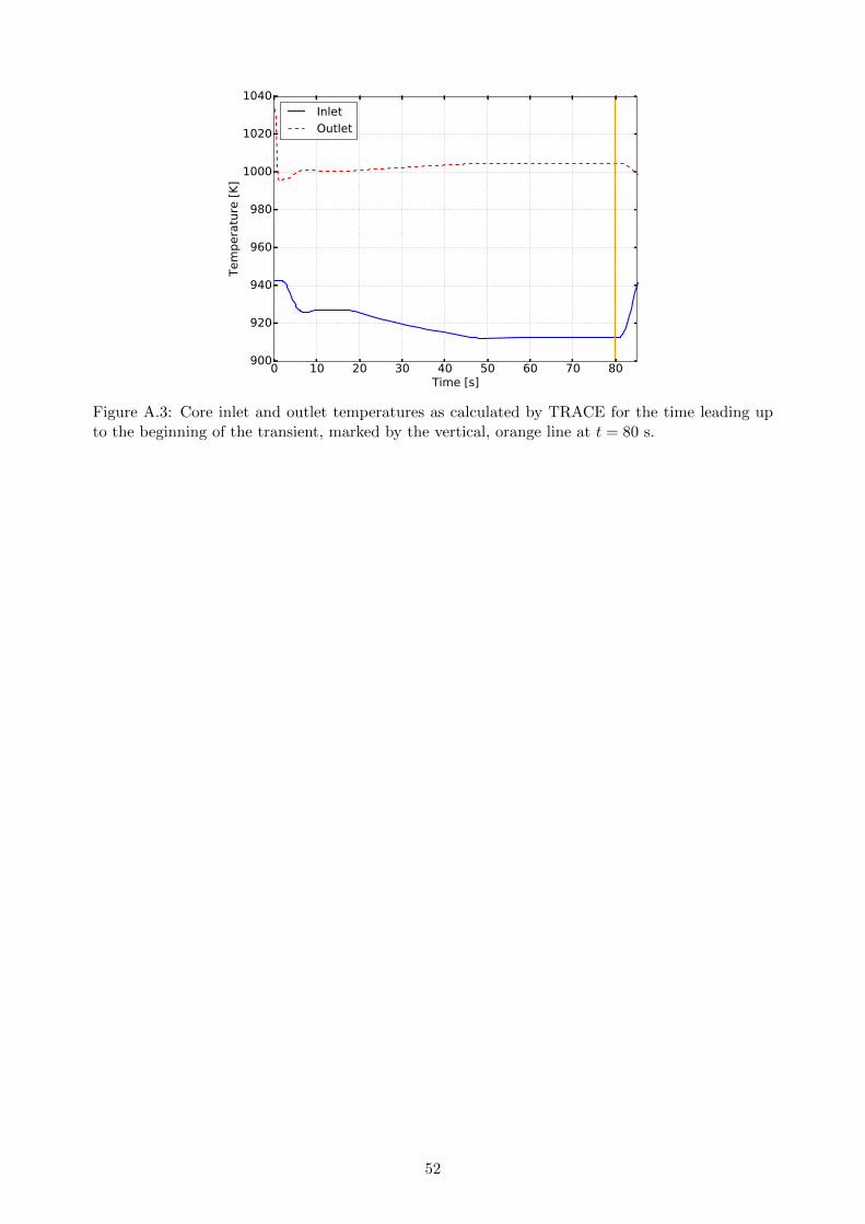
0 10 20 30 40 50 60 70 80Time [s]

900

920

940

960

980

1000

1020

1040

Tem

pera

ture

[K

]

Inlet

Outlet

Figure A.3: Core inlet and outlet temperatures as calculated by TRACE for the time leading upto the beginning of the transient, marked by the vertical, orange line at t = 80 s.

52

Acknowledgements

I would like to express my sincerest gratitude to the organisations that funded me while performing the presentedwork. This includes the GENTLE project that generously awarded me with a grant, as well as KIC InnoEnergy andStatens Lanekasse.

Furthermore, I would like to thank the Paul Scherrer Institut for kindly agreeing to host me for the duration of mymaster thesis project. Particular mention goes to Konstantin Mikityuk who accepted to serve as my supervisor, andwent on to perform that task admirably. Additional thanks to Jirı Krepel for originally proposing the project, toValentyn Bykov for patiently performing MCNP calculations for me, and to everyone else at PSI and in Wettingenfor assistance, discussions, laughs, and kindness.

This thesis has benefited tremendously from the tireless assistance of Matteo Zanetti, whose contributions are nowbeyond counting. Additional insights and motivation were provided by the participants to the 3rd SAMOFARProgress Meeting hosted in Grenoble, France.

53