Washington University in St. Louis Washington University in St. Louis Washington University Open Scholarship Washington University Open Scholarship Engineering and Applied Science Theses & Dissertations McKelvey School of Engineering Spring 5-15-2019 Coupled Correlates of Attention and Consciousness Coupled Correlates of Attention and Consciousness Ravi Varkki Chacko Washington University in St. Louis Follow this and additional works at: https://openscholarship.wustl.edu/eng_etds Part of the Cognitive Psychology Commons, Electrical and Electronics Commons, and the Neuroscience and Neurobiology Commons Recommended Citation Recommended Citation Chacko, Ravi Varkki, "Coupled Correlates of Attention and Consciousness" (2019). Engineering and Applied Science Theses & Dissertations. 441. https://openscholarship.wustl.edu/eng_etds/441 This Dissertation is brought to you for free and open access by the McKelvey School of Engineering at Washington University Open Scholarship. It has been accepted for inclusion in Engineering and Applied Science Theses & Dissertations by an authorized administrator of Washington University Open Scholarship. For more information, please contact [email protected].

Welcome message from author
This document is posted to help you gain knowledge. Please leave a comment to let me know what you think about it! Share it to your friends and learn new things together.
Transcript

Washington University in St. Louis Washington University in St. Louis
Washington University Open Scholarship Washington University Open Scholarship
Engineering and Applied Science Theses & Dissertations McKelvey School of Engineering
Spring 5-15-2019
Coupled Correlates of Attention and Consciousness Coupled Correlates of Attention and Consciousness
Ravi Varkki Chacko Washington University in St. Louis
Follow this and additional works at: https://openscholarship.wustl.edu/eng_etds
Part of the Cognitive Psychology Commons, Electrical and Electronics Commons, and the
Neuroscience and Neurobiology Commons
Recommended Citation Recommended Citation Chacko, Ravi Varkki, "Coupled Correlates of Attention and Consciousness" (2019). Engineering and Applied Science Theses & Dissertations. 441. https://openscholarship.wustl.edu/eng_etds/441
This Dissertation is brought to you for free and open access by the McKelvey School of Engineering at Washington University Open Scholarship. It has been accepted for inclusion in Engineering and Applied Science Theses & Dissertations by an authorized administrator of Washington University Open Scholarship. For more information, please contact [email protected].

WASHINGTON UNIVERSITY IN ST. LOUIS
School of Engineering & Applied Science
Department of Biomedical Engineering
Dissertation Examination Committee:
Eric C. Leuthardt, Chair
ShiNung Ching
Linda Larson-Prior
Dan Moran
Barani Raman
Coupled Correlates of Attention and Consciousness
by
Ravi Chacko
A dissertation presented to
The Graduate School
of Washington University
in partial fulfillment of the
requirements for the degree
of Doctor of Philosophy
St. Louis, MO
May 2019

© 2019, Ravi Chacko

ii
Table of Contents
List of Figures .............................................................................................................................................. iv
List of Tables ............................................................................................................................................... iv
Preface .......................................................................................................................................................... v
Acknowledgments ........................................................................................................................................ vi
Abstract ...................................................................................................................................................... viii
1) Introduction: Identifying Electrophysiological Correlates of Attention and Consciousness .................... 1
1.1 Brain Computer Interfaces (BCIs) ................................................................................................ 1
1.2 The Problem: BCI for Hemineglect: ............................................................................................. 3
1.3 The Question: How are attention and consciousness represented in the brain? ............................ 4
2) Background: Attention and Consciousness .............................................................................................. 8
2.1 Attention and inattention ............................................................................................................... 8
2.1.1 Hemineglect (HN) ................................................................................................................. 9
2.1.2 The Neuroanatomy of (In)Attention: .................................................................................. 10
2.1.3 Hemineglect Rehabilitation and a Rationale for BCI ......................................................... 12
2.1.4 Measuring Attention: The Posner Task............................................................................... 13
2.1.5 The Electrophysiology of Attention .................................................................................... 15
2.2 Consciousness ............................................................................................................................. 19
2.2.1 Defining Consciousness ...................................................................................................... 19
2.2.2 Sleep .................................................................................................................................... 21
2.2.3 Propofol Induced Loss of Consciousness (PILOC) ............................................................ 23
3) Methods: Measuring Phase-Amplitude Coupling................................................................................... 25
3.1 From Neuronal Firing to Scalp Recordings ............................................................................... 25
3.2 Phase-amplitude coupling (PAC) ................................................................................................ 30
3.3 Measuring PAC ........................................................................................................................... 31
3.4 Theory of PAC in neural oscillations .......................................................................................... 34
3.5 Challenges to PAC theory and measurement: Non-sinusoidal, Sharp Waves ............................ 35
3.6 Evidence for Phase-amplitude coupling in Attention and Consciousness ................................. 36

iii
4) Distinct Phase-Amplitude Couplings Distinguish Cognitive Processes in Human Attention ................ 38
4.1 Abstract ....................................................................................................................................... 38
4.2 Introduction ................................................................................................................................. 39
4.3 Materials and Methods ................................................................................................................ 41
4.4 Results ......................................................................................................................................... 47
4.5 Discussion ................................................................................................................................... 61
4.6 Supplemental Figures: ................................................................................................................ 65
5) Alpha-phase Coupling Distinguishes Mechanistically Distinct Unconscious States ............................. 68
5.1 Introduction ................................................................................................................................. 68
5.2 Results ......................................................................................................................................... 71
5.3 Discussion ................................................................................................................................... 76
5.4 Supplemental Data ...................................................................................................................... 78
6) Proof of Concept and Conclusion ........................................................................................................... 84
Appendix A: A Review of Rehabilitation Paradigms for Hemineglect ...................................................... 90
References ................................................................................................................................................... 92

iv
List of Figures
Title Page
3.1.1 Signal processing and analysis methods 38
3.1.2 Amplitude and phase of a complex signal 39
3.2.1 Phase-amplitude coupling measurement with modulation index 42
3.3.1 Importance of high frequency-for-amplitude wavelet bandwith 43
4.4.1 Task design showing analysis periods and behavioral results 57
4.4.2 Identification of distinct phase-amplitude coupling clusters 59
4.4.3 Functional classification of “spatial” and “behavioral” sites 62
4.4.4 Phase-preferences and relative PAC magnitude distinguishes frequency and class 64
4.4.5 PAC magnitude differences across task conditions 67
4.4.6 Transient waves are behaviorally relevant and coupled to 7.2 Hz phase 69
4.6.1 Supplemental figures 75
5.2.1 Double dissociation of PAC by frequency pair and sleep state 81
5.2.2 TABL PAC decresases during SWS but increases during PLOC 83
5.2.3 Increased theta- and alpha-phase PAC is not caused by changes in power 85
5.4.1 Consistency of double dissociation across patients 88
5.4.2 Delta-phase PAC increases and alpha-phase PAC decreases with NREM stage 92
6.1.1 Log-loss classifier performance for left vs right target locations 95
6.1.2 Adding a dimension to the spectrum of consciousness 99
List of Tables
Table 1: NIH stroke scale for quantification of neglect 18

v
Preface
It has been an honor and a privilege to study the brain at Washington University in St.
Louis. I have been fortunate to work with researchers across many disciplines, such as
biomedical engineering, experimental and theoretical neuroscience, cognitive neuropsychology,
neurosurgery, neurology, neuronal modelling, anesthesiology, hypnology, machine learning,
probability, signal processing and computer science. The following work will touch on high-
level concepts from all these fields to describe electrophysiological correlates of attention and
consciousness. Chapter 1 supplies the motivation for our thesis and includes a rationale for the
topics discussed. The goal of this project was to better understand the mesoscopic
electrophysiology of attention so that it can be used in the rehabilitation of attentional disorders
such as hemispatial neglect. This goal led to a study of phase-amplitude coupling and its
relationship to attention and arousal. Chapter 2 is a background on attention, sleep and
anesthesia. Chapter 3 reviews the methodological choices we make for measuring phase-
amplitude coupling (PAC). Chapter 4 reports our experimental findings on how different PAC
frequency clusters relate to different aspects of human attention. Chapter 5 reports findings on
differences in PAC between conscious and two distinct unconscious states. We conclude with a
discussion of how these findings can be used in future work to implement brain computer
interfaces for rehabilitating hemispatial neglect in Chapter 6.

vi
Acknowledgments
I am grateful for the many discussions with my fellow graduate students, including Nick
Szrama, Mrinal Pahwa, Carl Hacker, Ammar Hawasli, Jarod Roland, Mohit Sharma, David
Bundy, Joey Humphries, Andy Daniels, DoHyun Kim, Josh Siegel and Amy Daitch. Without
them this research would never have come to fruition. I greatly appreciate the efforts of my
mentor, Eric Leuthardt, pushing me to consider new research topics. I appreciated the
complementary mentorship of Maurizio Corbetta and Gordon Shulman, especially when
discussing meaning of our experimental findings. I also enjoyed discussing the theoretical
underpinnings of our modelling work and what the definition of “is” is with ShiNung Ching. I
am grateful to the additional mentorship afforded to me by Linda Larson-Prior, Barani Raman,
Dan Moran and Andy Mitz, who all pushed me to be a better scientist and engineer. I consider
the time spent bantering about theoretical neuroscience priceless. I especially enjoyed
questioning the foundational premises of my work, and of many other people’s work, as it gave
me a great deal of perspective. Finally, I must thank my father, for coaching me through a PhD,
my mother, for understanding me, my brother, for being my inspiration and my fiancé, for
encouraging me through the tough times while accomplishing her own incredible feats.
Ravi Chacko
Washington University
May 2019

vii
This work is dedicated to my dear parents.

viii
Abstract
ABSTRACT OF THE DISSERTATION
Coupled Correlates of Attention and Consciousness
by
Ravi Varkki Chacko
Doctor of Philosophy in Biomedical Engineering
Washington University in St. Louis, 2019
Eric C. Leuthardt, Chair
Introduction: Brain Computer Interfaces (BCIs) have been shown to restore lost motor function
that occurs in stroke using electrophysiological signals. However, little evidence exists for the
use of BCIs to restore non-motor stroke deficits, such as the attention deficits seen in
hemineglect. Attention is a cognitive function that selects objects or ideas for further neural
processing, presumably to facilitate optimal behavior. Developing BCIs for attention is different
from developing motor BCIs because attention networks in the brain are more distributed and
associative than motor networks. For example, hemineglect patients have reduced levels of
arousal, which exacerbates their attentional deficits. More generally, attention is a state of high
arousal and salient conscious experience. Current models of consciousness suggest that both
slow wave sleep and Propofol-induced unconsciousness lie at one end of the consciousness
spectrum, while attentive states lie at the other end. Accordingly, investigating the
electrophysiology underlying attention and the extremes of consciousness will further the
development of attentional BCIs.

ix
Phase amplitude coupling (PAC) of neural oscillations has been suggested as a
mechanism for organizing local and global brain activity across regions. While evidence
suggests that delta-high-gamma PAC, which includes very low frequencies (i.e. delta, 1-3 Hz)
coupled with very high frequencies (i.e. gamma 70-150 Hz), is implicated in attention, less
evidence exists for the involvement of coupled mid-range frequencies (i.e. theta, 4-7Hz, alpha: 8-
15 Hz, beta: 15-30 Hz and low-gamma: 30-50 Hz, aka TABL PAC). We found that TABL PAC
correlates with reaction time in an attention task. These mid-range frequencies are important
because they can be used in non-invasive electroencephalography (EEG) BCI’s. Therefore, we
investigated the origins of these mid-frequency interactions in both attention and consciousness.
In this work, we evaluate the relationship between PAC to attention and arousal, with emphasis
on developing control signals for an attentional BCI.
Objective: To understand how PAC facilitates attention and arousal for building BCI’s that
restore lost attentional function. More generally, our objective was to discover and understand
potential control features for BCIs that enhance attention and conscious experience.
Methods: We used four electrophysiological datasets in human subjects. The first dataset
included six subjects with invasive ECoG recordings while subjects engaged in a Posner cued
spatial attention task. The second dataset included five subjects with ECoG recordings during
sleep and awake states. The third dataset included 6 subjects with invasively monitored ECoG
during induction and emergence from Propofol anesthesia. We validated findings from the
second dataset with an EEG dataset that included 39 subjects with EEG and sleep scoring.
We developed custom, wavelet-based, signal processing algorithms designed to optimally
calculate differences in mid-frequency-range (i.e. TABL) PAC and compare them to DH PAC
across different attentional and conscious states. We developed non-parametric cluster-based

x
permutation tests to infer statistical significance while minimizing the false-positive rate. In the
attention experiment, we used the location of cued spatial stimuli and reaction time (RT) as
markers of attention. We defined stimulus-related and behaviorally-related cortical sites and
compared their relative PAC magnitudes. In the sleep dataset, we compared PAC across sleep
states (e.g. Wake vs Slow Wave Sleep). In the anesthesia dataset, we compared the beginning
and ending of induction and emergence (e.g. Wake vs Propofol Induced Loss of Consciousness)
Results: We found different patterns of activity represented by TABL PAC and DH PAC in both
attention and sleep datasets. First, during a spatial attention task TABL PAC robustly predicted
whether a subject would respond quickly or slowly. TABL PAC maintained a consistent phase-
preference across all cortical sites and was strongest in behaviorally-relevant cortical sites. In
contrast, DH PAC represented the location of attention in spatially-relevant cortical sites.
Furthermore, we discovered that sharp waves caused TABL PAC. These sharp waves appeared
to be transient beta (50ms) waves that occurred at ~140 ms intervals, corresponding to a theta
oscillation. In the arousal dataset DH PAC increased in both slow wave sleep (SWS) and
Propofol-induced loss of consciousness (PILOC) states. However, TABL PAC increased only
during PILOC and decreased during SWS, when compared to waking states. We provide
evidence that TABL PAC represents “gating by inhibition” in the human brain.
Conclusions: Our goal was to develop electrophysiological signals representing attention and to
understand how these features explain the relationship between attention and low-arousal states.
We found a novel biomarker, TABL PAC, that predicted non-spatial aspects of attention and
discriminated between two states of unconsciousness. The evidence suggested that TABL PAC
represents inhibitory activity that filters out irrelevant information in attention tasks. This
inhibitory mechanism of was confirmed by significant increases in TABL PAC during Propofol

xi
anesthesia, when compared to SWS or waking brain activity. We conclude that TABL PAC
informs the development of electrophysiological control signals for attention and the
discrimination of unconscious states.

1
1) Introduction: Identifying Electrophysiological
Correlates of Attention and Consciousness
“Every speculative enterprise which he undertook, and they were many and various, was carried
to sure success by the same qualities of cool, unerring judgment, far-reaching sagacity, and
apparently superhuman power of organizing, combining, and controlling, which had made him in
politics the phenomenon of the age” – The Ablest Man in the World, Edward Page Mitchell, 1884
In Edward Page Mitchell’s short story, “The Ablest Man in the World” a doctor describes
treating a sick Russian baron and stumbling on a curious finding. Underneath the baron’s skull
cap, a silver dome covered a clockwork brain. The baron was born with neurological deficits and
a Russian doctor with skill in watchmaking designed a clockwork brain to fix them. Not only did
it fix his deficits, but it gave him superhuman powers. For more than a century human have
imagined using devices to improve neurological function. This work extends this effort by
understanding how the brain represents attention and certain aspects of consciousness to treat
disease and augment human cognition.
1.1 Brain Computer Interfaces (BCIs) The purpose of a BCI is to decode the neural activity associated with a behavior so that the
behavior can be recreated or augmented. BCIs are designed by modelling and predicting brain
activity with high accuracy in over short time periods. To do this, we typically record brain
activity while subjects repeat a task. We then model the neural activity that represents important

2
aspects of the task and use that model to predict behavior. For example. a paralyzed patient with
an injured spinal cord has a functioning motor cortex. We might ask the patient to think about
moving their hand while recording brain activity from their motor cortex. After recording enough
data, a model can be created to predict when the patient is thinking about moving his hand.
Ultimately a robotic hand can complete the required behavior after the model makes an
appropriate prediction, thus recreating the patient’s lost neurological function. BCIs typically
consist of three elements, 1) a neural interface, 2) a computational processing module and 3) an
output. While BCIs have made progress in the restoration of motor deficits in stroke and
paralysis1–4, they have not succeeded in improving cognitive functions like the ones in Mitchell’s
quote above. Here we focus on the cognitive function called attention. Developing BCIs to
augment attention would benefit stroke patients with Hemineglect.
Hemineglect is an attention disorder and the motivation for this thesis. Previously, BCIs have
been used to improve hemiparetic stroke syndromes, which incorporate movement disorders1.
When we attempted to apply BCI principles from movement disorders to attention disorders
several issues became salient. Compared to movement, attention is a higher order cognitive
function that involves more brain networks working in concert. For example, if you call out to
someone and they don’t respond, it could be because (A) they don’t perceive you calling them
(e.g. they’re deaf), (B) they don’t have the ability to execute a response (e.g. they’re paralyzed)
or (C) there is something wrong with their brain’s ability to convert a perception of you calling
them to a response (e.g. Hemispatial neglect). Our goal was to understand the
electrophysiological correlates of attention, which transforms sensory perceptions into
measurable behaviors, so that they can be used to repair neurological deficits. The following two

3
chapters discuss how a clinical and engineering motivation required the scientific approach we
pursued.
1.2 Problem: BCI for Hemineglect: Hemineglect (HN) describes the inability to attend to one half of space (i.e. hemifield) that
typically follows a right-brain stroke. These patients fail to shave one half of their face, dress one
half of their body and draw one half of pictures they are given to copy. They also have slower
response speeds to stimuli in both hemifields and suffer from reduced levels of arousal. HN
occurs in 25-30% of all stroke patients, 10-13% of left hemisphere strokes and 40-82% of right
hemisphere strokes5–9. This amounts to roughly 200,000 people a year. Decades of research have
yielded theories that explain elements of HN10–13, but meta-analyses conclude that there currently
is no effective rehabilitation treatments for HN14,15. The goal of this work was to develop
innovations in HN rehabilitation using BCI methodologies. If we can understand which signals
explain lateralized attention and response speed, we can teach HN patients to increase their
output of that signal. To develop these BCIs we proposed the development of attentional control
signals, or electrophysiological signatures of attention.
We focus on electrophysiological signatures because they can be used with
electroencephalography (EEG) neurofeedback. EEG uses non-invasive scalp electrodes that
record electric potential. While an EEG neurofeedback device is the ultimate goal, this research
focuses on electrocorticography (ECoG), which uses surgically implanted electrodes on the
surface of the brain. ECoG is prescribed for epilepsy patients, who have failed conservative
treatment, in order to localize the origins of seizures. The advantage of ECoG is that the signal is
less noisy and more spatially specific than EEG signal. ECoG also records higher frequencies

4
than EEG. However, our goal will be to focus on features that can eventually be used with EEG
feedback, which rules out frequencies above 50 Hz.
Finally, ideal attentional control features will be measurable on single trials. If an EEG
neurofeedback paradigm for hemineglect mirrors its motor stroke counterpart, then it will require
the patient to practice. This means many repeated trials. The neurofeedback device must tell its
operator how well he or she attended during the last trial. If we cannot compute this value
quickly, then the operator won’t know how to improve their attention. This is a consequence of
operant conditioning, where the strength of a behavior is modified by reward or punishment (i.e.
feedback).
In summary, our goal is to develop attentional control features that will serve an EEG
neurofeedback device. It must use frequencies below 50 Hz and must be able to detect whether
the subject paid attention on a single trial. In the end, a hemineglect patient will wear an EEG
headset while playing a computer game that challenges their attention. On trials where they
attended properly, they will be rewarded. On trials where they fail to attend, they will not be
rewarded. By repeatedly playing this game, they will learn what promotes and prevents attention.
But what does it mean to attend properly? Hemineglect patients have more than one deficit. Not
only are they unable to attend to one half of space as well as the other, they also have deficits
that exist on both halves of space16,17. Furthermore, the colloquial usage of the word “attention”
doesn’t always fit the scientific and clinical understanding. Therefore, before we set out to find
attentional control signals, we will first understand the components of attention.
1.3 The Question: How are attention and consciousness represented in the brain? To begin to understand the lateralized attention deficit in hemineglect, think of your attention
like a spotlight. Much of the time it moves around with your gaze. However, just as your eyes

5
can scan words on a page without absorbing any of its meaning, your attention can move
independently of your gaze. To convince yourself, fixate on the red dot below after completing
this passage and avoid looking directly at the items to the left of the right of the dot. Try
attending to the left of the dot without looking away from the dot. You’ll notice that item to the
left of the page will become more salient and you will make out its identity more easily. Notice
how shifting your attention to the left of the dot (again without breaking fixation) makes it more
difficult to resolve the stimulus to the right of the page.
.
This is because attention is a limited resource, or a “limited-capacity spotlight”18. When it
shines in one part of the visual field, it does not shine in another. HN patients fail to attend to one
half of space. This is known as the “spatial” deficit in HN. EEG correlates of lateralized
attentional shifts have been shown in the alpha (8-13 Hz) frequency19. However, alpha power
did not discriminate left and right shifts in attention much better than chance. Furthermore,
lateralized attention deficits aren’t the only attentional deficits in hemineglect.

6
In healthy subjects, attention is often measured using response times (RT)20–22. A subject
typically attends to a location in space, then respond to stimuli that appear at that location or at
an unattended location. RT measures the entire mental sequence of deploying attention, orienting
it, sustaining it, sensing or perceiving the relevant stimuli, processing it, then planning and
executing a motor response. In addition to the markedly slower responses (i.e. higher RTs) to
stimuli in their neglected hemifield (i.e. the “spatial” deficit), HN patients also have a slower
response to all stimuli, regardless of where it occurs23. This is known as the “non-spatial” deficit
in neglect. What’s more, depending on the location of the stroke, an HN patient may have
different ratios of “spatial” and “non-spatial” deficits in neglect24. Therefore, we must be careful
to distinguish between “spatial” and “non-spatial” aspects of attention. But “non-spatial”
attention is not the only cognitive function to influence RT. For example, when you are drowsy
you will respond more slowly to all stimuli. Furthermore, if you are distracted by some other
task, you will also respond more slowly to all stimuli. Therefore, we must understand how
attention is related to consciousness more generally.
Consciousness refers to a multifaceted concept, but we will initially describe it with two
dimensions. The first is arousal or wakefulness, the second is awareness or experience25. In
clinical settings, the first dimension is useful because distinguishes levels of brain injury or
coma. The second dimension is the subject of philosophical writings and psychopsychics
research. Most of the cognitive states discussed below differ along both axes of arousal and
awareness. For example, a state of attention is a state of high arousal and high awareness
compared to resting wakefulness. Conversely, sleep is a state of low arousal and low awareness.
In the following chapters, we will compare what we learned from attentive states to two states of
lost consciousness, slow-wave sleep (SWS) and Propofol-induced loss of consciousness

7
(PILOC). We use these two states because SWS has a well-studied neurophysiology and PILOC
has a well-known mechanism of action.
In summary, our engineering goal of developing a BCI for Hemineglect requires the
scientific pursuit of measuring physiology associated with the abstract concepts of attention and
consciousness. Therefore, we will study attention as it relates to a) lateralized shifts in attention
and b) reaction time (RT), with the caveat that RT are generated by multiple cognitive systems.
Furthermore, we will investigate consciousness across two states, SWS and PILOC. Contrasting
brain activity across these variables and states underlies our scientific findings.

8
2) Background: Attention and Consciousness
Attention is a cognitive1 selection mechanism that selects an object or idea for further
processing. A colloquial example of inattention is when one attempts to read words on a page
and realizes, at the end of a passage, that the passage wasn’t read or comprehended. Even though
eyes scanned words on the page, the cognitive function called attention did not select the words
for language comprehension. Thus, the object (i.e. words) that one’s eyes selected was not
selected by one’s brain for further processing (i.e. comprehension). With respect to spatial
attention, where you look is commonly where you attend. But as the example demonstrates, this
is not always the case. A behavioral paradigm that measured this type of inattention is the Posner
cueing task 26. As this task is central to the study described in Chapter 4, we will use it to
elaborate neuropsychological concepts around attention and clinical sequalae of lost attentional
function in hemineglect (HN).
2.1 Attention and inattention
William James’s famously said “[Attention] is the taking possession by the mind, in clear
and vivid form, of one out of what seem several simultaneously possible objects or trains of
thought, localization, concentration, of consciousness are of its essence.” Simply put, attention is
a cognitive function that selects what the brain thinks about. This description, however, is
lacking because we have an incomplete understanding of how the brain processes “items or
trains of thought” that have been selected. Attention studies typically measure behaviors as a
1 Cognition is the mental action or process of acquiring knowledge and understanding through thought, experience, and the senses. Or a result of this; a perception, sensation, notion, or intuition.

9
proxy for cognitive processing. An experiment will manipulate inputs (e.g. items to be selected)
and measure outputs (e.g. actions required to complete the task). We therefore study how brain
transforms sensory inputs into motor outputs. Unfortunately, this “black box” model of attention
is also vague. Therefore, we will motivate our definition of attention by two HN deficits that are
measurable with the Posner spatial cueing task. The first deficit is in spatially lateralized aspects
of attention, the second deficit is in non-spatial aspects of attention.
2.1.1 Hemineglect (HN)
Hemineglect (a.k.a. neglect, hemispatial neglect and spatial neglect) is a stroke syndrome that is
most commonly diagnosed by a lateralized deficit in attention. HN is diagnosed as hemi-
inattention (Table 1), a failure to orient, or respond to stimuli on one side of space that cannot be
explained by a visual or motor deficit8,27. Typically, right sided parietal strokes lead to a left
sided hemineglect. A patient with profound hemineglect may orient their head to the right of
center and may not use their left hand.
Table 1: NIH Stroke scale for the quantification of (Hemi)neglect. Extinction is when
hemineglect symptoms occur only when stimuli are presented simultaneously in both
hemifields.
The “spatial” or “lateralized” deficits in neglect are most striking. HN patients may shave
only one half of their face or dress only one side of their body. It’s important to note that HN is
not a visual or tactile deficit. Patients can see into the neglected hemispace and feel their

10
neglected hemibody when cued to do so. Furthermore, it is not a motor problem, as patients can
move their limbs and respond to directions. Therefore, it is a problem with attention networks in
the brain that coordinate sensory inputs with motor outputs to execute goal-oriented behaviors.
Patients with HN may not feel anything is wrong. It is as if their world has shrunk to half the
size, but this shrunken world has stretched to occupy the entire space. What’s more, HN doesn’t
only affect present experiences, it also interacts with memory. One hemineglect patient was
asked to imagine standing in their town square and recall all the buildings he could. He dutifully
recalled all the buildings on the right of where he was standing. Next, the clinician asked this
patient to turn around, in his imagination, and repeat the task. Again, the patient recalled all the
buildings to his right. Without realizing it, the patient had recounted all the buildings in the
square, but at any given positioning he could only recall one side. This points to the multifaceted
nature of attention, beyond its effects on stimulus perception and motor behavior23.
“Non-spatial” HN deficits are not lateralized to one side. HN patients are slower to respond
to any stimuli, regardless of the side they are stimulated on. They also suffer deficits in sustained
attention and working memory. These deficits have been shown to predict clinical outcome
independently of lateralized deficits16. Furthermore, “spatial” and “non-spatial” deficits in
neglect have been associated with different cortical lesions, which have furthered our
understanding of attentional networks in the brain. To summarize, HN is a stroke syndrome that
causes hemi-inattention which effects both spatial (or lateralized) and non-spatial aspects of
attention.
2.1.2 The Neuroanatomy of (In)Attention:
Typically, HN patients sustain damage to their right hemisphere and neglect the left
hemifield. Cortical and subcortical lesions at many locations can cause HN. These include the

11
inferior parietal lobule, superior temporal gyrus, middle frontal gyrus, inferior frontal gyrus,
arcuate fasciculus and superior longitudinal fasciculus28–30. Animal studies have implicated
subcortical structures like the hypothalamus31. fMRI studies of HN patients reveal disrupted
dorsal and ventral attention networks (DAN and VAN)24. Compared to healthy subjects, Inter-
hemispheric functional connectivity in these networks decreased in HN patients, while intra-
hemispheric activity between networks increased32,33. HN lesions often coexist with visual,
motor, limbic and frontal lesions, which complicates treatment and diagnosis.
The dorsal attention network (DAN) includes the Frontal Eye Fields (FEF), sensorimotor
cortices and parietal reach regions. It is involved in preparing and executing top-down, or goal-
oriented, attentional shifts. The ventral attention network (VAN) includes the Fusiform Face
Area, the amygdala and other fronto-ventro-temporal structures. This system is specialized for
detection of behaviorally salient stimuli and is lateralized to the right brain9,11. Lesions that cause
HN usually affect both dorsal and ventral streams functionally, but damage to one system may
interact with the other23,34.
Direct evidence for the locus of spatial attention comes from a neurosurgical
experiment35. During tumor resection surgery, the superior occipitofrontal fasciculus (SOF) was
stimulated during a line bisection task. In this task, a subject is asked to divide a horizontal line
in half with an orthogonal line. Biases in spatial awareness are measured by how far away from
the midline the subject’s bisection lies. In this experiment, the subjects’ bisections were shifted
to the right when the SOF was stimulated. This suggests that neural information transferred
between frontal and parietal regions is integral for spatial awareness or attention. This finding
references well with a third resting state network, the fronto-parietal network (FPN), which is
implicated in goal-directed cognition36.

12
To summarize, HN can result from lesions to the DAN, VAN and FPN networks in the
brain. These networks contribute to localization of attention, identification of stimuli and goal-
directed behaviors respectively. Together, these begin to explain the constellation of deficits
found in HN. Patients have difficulty orienting towards relevant stimuli, processing them and
responding to them. They also have difficulty maintaining attention to complete tasks. Unlike the
motor network, attention spans multiple lobes and networks in the brain, underscoring its
distributed functionality in the brain.
2.1.3 Hemineglect Rehabilitation and a Rationale for BCI
Before developing control features for an HN BCI, we first reviewed current
rehabilitation strategies and provide a rationale for why a BCI approach will work. Rehabilitation
strategies for HN have been divided into top down and bottom up approaches. Top down
approaches develop strategies to compensate for deficits. For example, repeatedly instructing a
patient to remain alert improves HN deficits24. Bottom up approaches improve symptoms by
altering the perceptual experience of the patient. These include using prism goggles, pouring
cold water in the ear and virtual reality approaches (see Appendix A for a review of
rehabilitation approaches). A BCI approach to HN rehabilitation is likely to succeed for five
reasons. First, existing interventions demonstrate how attentional deficits are transiently
recoverable7,14,37. Second, BCI approaches make use of computer games that can combine top-
down and bottom-up methods. Third, many patients can eventually recover from neglect7, which
again suggests that the deficit is recoverable. Fourth, BCI approaches can be administered at
home and dosed more regularly than interventions that require a therapist. Fifth, successful BCI
treatments to improve attentional deficit in attention-deficit hyperactivity disorder exist38, which
suggests other attention deficits are recoverable with similar methods. The first step in this BCI

13
approach is to create a model of how electrophysiological signals represent attention. This itself
is a challenge because its relatively difficult to visualize attention. To help with this, we use the
Posner task, which measures both spatial and non-spatial aspects of attention. In Chapter 4, we
will use the Posner task to develop control signals for BCI rehabilitation.
2.1.4 Measuring Attention: The Posner Task
Michael Posner begins his work “Orienting of Attention” struck by “the idea that a hidden
psychological process like the formation of a thought might be rendered sufficiently concrete to
be measured”26. Measuring hidden psychological processes is perhaps a prerequisite to
Mitchell’s vision, quoted at the beginning of Chapter 1. Posner’s goal was to use the concept of
spatial attention to corroborate human psychological experiments with physiological animal
experiments. He broke down the process of responding to cued stimuli into four steps.
Orienting is the aligning of attention with the source of sensory input or internal semantic
structure stored in memory
Detecting is when a stimulus reaches a level of representation in the nervous system where
the individual can report its presence
Locus of Control (Intrinsic/Extrinsic) is whether orienting was caused by an external
stimulus (e.g. a loud sound behind you) or out of one’s own volition (e.g. purposefully
reading this manuscript)
Covert attention is attending to a location in space where your eyes are not fixated (i.e.
looking out of the corner of your eye)
Posner used these concepts to analyze a cued spatial attention task. In the task, a participant
began every trial by fixating on a central location. A central cue appeared that indicated whether

14
a stimuli would appear on the left or the right of screen. Most of the time, the cue indicated
where the target would appear (valid trials). This ensured that the participant attended to the cued
location. On a small number of trials, however, the cue pointed one direction and the target
appeared in the opposite location (invalid trials). Posner found, that valid trials yielded faster
reaction times than invalid trials. Posner found that he could measure where attention was being
allocated by quantifying the time necessary to reallocate it. When keeping eyes centrally fixated,
the participant shifted her “spotlight of attention”, independently from the location of eye
fixation, toward the cued location. On the rare invalid trial, when the target appeared in an
uncued location, the participant was forced to re-orient attention to the uncued location. Longer
reaction times quantified this unseen cognitive maneuver. This experiment validated the idea that
attention is limited: when attending to a location, one is simultaneously not attending to another
location. No surprisingly, the deficits experienced by HN subjects can also be measured with the
Posner task.
Rengachary et al. found that the Posner task captured both spatial and non-spatial aspects of
HN. First, HN subjects were slower to respond to trials in their neglected visual field. Healthy
subjects respond with equal RTs to targets on either side of their visual field. Second, HN
subjects are slower to respond to all stimuli compared to healthy controls, regardless of which
side it was on. Furthermore, these differences scaled with chronicity of the injury. Acute patients
showed larger deficits in the Posner task than chronic patients37. The difference between reaction
times in the left and right visual field marks the lateralized, spatial deficit in HN. The increased
reaction times (RTs) for both sides indexed the non-spatial deficit in HN. Furthermore,
Rengachary et al. also found that the Posner task was more sensitive to detecting clinically
relevant aspects of HN than standard clinical testing39. In summary, the Posner task measures

15
attention and has been shown to measure the extent of HN deficits. In Chapter 4 we use the
Posner task to interrogate the electrophysiological correlates of attention. We first review what
has been previously demonstrated in the electrophysiological attention literature.
2.1.5 The Electrophysiology of Attention
Electrophysiological correlates of spatial attention have been investigated in multiple
recording modalities. Single unit (i.e. neuron) recordings measure firing rates of neurons from
electrodes implanted directly into the cortex. Single unit studies provide fine grain detail on how
neurons change their firing rates based on changing parameters. EEG experiments study a larger
network of neurons as electrodes are placed on the scalp. These experiments measure slower
oscillatory activity from larger swaths of the brain than single neuron experiments. Additionally,
the visual system is organized contralaterally and in topographical maps. Visual information
from the left visual field is primarily decoded in the right cerebral hemisphere and vice versa.
Within each hemisphere, there is a map of visual space. Experimenters use these maps to
pinpoint what region of space a neuron corresponds to, then probe that region in space with
stimuli in a task.
Correlates of Lateralized Attention: Bisley and colleagues found that neuronal firing in
homologous (i.e. on both sides of the brain) areas of the lateral intraparietal sulcus (LIP)
correlated with lateralization of covert attention40. The LIP has been associated with tracking
motion and moving eye gaze to relevant locations in space. Using a cued attention task similar to
the Posner task, Bisley et al. found that when monkeys directed attention to the left, neurons in
the right LIP fired at a higher rate than those in the left LIP. Thus the locus of attention
correlated with the difference between left and right LIP neuronal firing rates. Similarly, EEG
studies in healthy subjects have shown differential encoding of lateralized attention using alpha

16
power. In cued spatial attention tasks, the normalized difference in alpha activity over
homologous parieto-occipital regions correlated with the locus of attention19,41. The authors
hypothesized this “alpha index” increases the signal-to-noise ratio of the neural control of spatial
attention42. This signal, however, provided relatively low predictive power about the locus of
attention on single-trials. Unfortunately, ECoG doesn’t cover both sides of the brain because
ECoG grids are typically applied to one cerebral hemisphere. Nevertheless, these experiments
provide candidate control signals for the neural correlates of lateralized attention for our studies.
In summary, multimodal experimental evidence suggests that lateralization of spatial attention is
encoded in differences of local neuronal activity and alpha oscillations across cerebral
hemispheres.
Correlates of Reaction Time: Electrophysiological research on non-spatial aspects of
attention (i.e. RT) are much broader than efforts to uncover lateralized attention phenomena.
This is because reaction time (RT) measures a long sequence of neural processes. For example, a
subject might take longer to identify a stimulus or that same subject might execute a slower
motor response. Both will result in longer reaction times. Single unit studies have shown that the
neural substrates of RT begin with single neurons in the primary sensory regions. When a
monkey passively listens to auditory stimuli, the neurons in that monkey’s primary sensory
regions are less active than when a monkey actively listens to the same stimuli for the purpose of
responding to them20. The finding that attention increases the basal firing rates of sensory
neurons has been shown across sensory domains 43. This provides evidence that early processes
in the sequence of neural events leading to a behavioral response are modulated by attention.
Historic EEG studies investigated neural activity just before the initiation of a response and
discovered what’s known as the “bereitschaftspotential”. The bereitschaftspotential is alpha (8-

17
13 Hz) oscillatory activity that increases in power just prior to movement. This rhythm has been
exploited for motor BCIs because it will remain intact even if the spinal cord is severed. If an
individual is paralyzed but has an intact brain, the bereitschaftspotential will predict when that
individual desires to move. More generally, EEG correlates of reaction time have been found in
the alpha and beta (13-30 Hz) frequency ranges. In a dual modality, auditory and visual, reaction
time task, Senkowski et al. found that beta power correlated with RT in multiple areas in the
brain, including frontal, occipital and sensorimotor cortices. Importantly, the correlation between
beta and RT was negative, which means the higher the beta activity the faster the reaction time.
The authors suggest that beta activity marks increased activation associated with multisensory
processing44. To summarize, RT measures a host of processes that transform the perception of a
stimulus to an action. However, multiple lines of evidence suggest that the measured brain
activity correlates with future reaction times.
Relationship between neural oscillations and attention: We previously discussed how
alpha oscillatory activity correlates with the direction of cued attention and beta oscillatory
activity correlates with RTs. Now we discuss why attention might be related to oscillatory
activity in the first place. To do this we first discuss two additional experiments and a theory. In
the first experiment, visual and audio oddball tasks were interleaved, and a monkey was required
to attend only to visual or auditory stimuli. The goal of the task was to respond to a low
frequency audio or visual “oddball” amongst high frequency stimuli (i.e. (auditory) respond to
the rare “beep” and ignore the frequent “boop” sounds or (visual) respond to the rare green
square while ignoring the frequent red squares). When the monkey attended to the visual stimuli,
neural oscillations entrained to the timing of the task creating high delta (1-3 Hz) power and
gamma (75-100 Hz) activity increased during specific phases of the delta oscillation. Gamma

18
activity is believed to represent local neuronal firing. This effect only occurred in the visual
cortex when the monkey attended visual stimuli. When the monkey attended auditory stimuli, the
effect occurred in the auditory cortex. When attention was deployed to a sensory system, the
corresponding brain region oscillated. Then, the local neuronal activity in that region became
entrained to the ongoing oscillation. The authors suggest that low frequency oscillations are
responsible for transiently increasing the excitability of neurons in primary sensory cortices in
order to maximize perception of rhythmic stimuli45. Delta essentially amplified rhythmic stimuli
by entraining the brain to their timing.
The finding that neural oscillations relate to attention is consistent with findings that the
phase of low frequency oscillations predict visual perception46,47. Perception can be measured by
asking subjects whether they have seen a specific stimulus or not. The phase of an oscillation is a
description of where that oscillation is in its cycle. The phase starts at 0 and completes a full
cycle at 360 (i.e. 2 pi). In multiple experiments, authors have found that the phase of ongoing
theta (3-7 Hz) or alpha oscillations predicts whether a stimulus is detected or not46,47. If a visual
stimulus is presented at the 180-degree phase of the oscillation, the stimulus is more likely to be
detected. Beyond perception, interactions between low frequency phase and high frequency
amplitude have also been shown to predict reaction time. One study showed that the phase
locking value (PLV) between delta/theta and gamma bands correlated with reaction times48.
These findings suggest that perception and performance may depend on parcellated periods of
time that are created by oscillations.
Our subjective experience of the world is a continuous one. We do not see time moving in
steps or space represented as pixels. However, this is an illusion created by the brain. The visual
system is represented by individual neurons in the retina that correspond to discrete sections of

19
the visual field. Despite this, we visualize a continuous visual field. Why then, should time be
any different? Discrete attentional sampling was proposed in the “Active Sensing” hypothesis13.
The authors suggest that humans may perceive our environment similarly to robots that
discretely sample signals from the environment. The strongest example of this is in olfaction
where sensing a smell is intimately linked with respiration. When a mouse inspires, it is more
likely to smell something salient, therefore the sensation of smell is not passive, but actively
generated. Visual attention can be moved independently of eye muscles, making the active
sensing hypothesis less obvious in visual attention. However, the findings that perception
depends on the phase of ongoing oscillations suggests that cognitive rhythms may underlie visual
sampling. Critics of this hypothesis suggest that the 1/f, or scale-free, distribution of brain
activity allows for continuous temporal sampling49. These theoretical arguments underscore the
difficulty in understanding subjective human experience. However, “experience” is one way to
define consciousness and consciousness is a cognitive state that we can manipulate and measure.
2.2 Consciousness
2.2.1 Defining Consciousness
There are at least two ways to define consciousness, “experience/awareness” or
“arousal/wakefulness”, and both relate to attention. In hemineglect, both the awareness of space
and general levels of arousal are affected. In Chapter 5 we will report novel findings on the
electrophysiological correlates of slow wave sleep and Propofol-induced loss of consciousness.
Even though arousal and experience are both reduced in unconscious states, we will review these
terms separately at first to better understand the meaning of consciousness.

20
Awareness: Many have had the experience of driving while thinking about something other
than driving. If a driver’s attention is directed to sending a text message or singing a song, he
will be less aware of his environment. However, a driver can lack awareness even while looking
at the road, provided something else occupies his thought. Awareness references the subjective
experience of reality, and is difficult to measure. For example, patients with “locked-in
syndrome” (LIS) have functional brain activity, but are unable to move their body. LIS is not a
disorder of consciousness, it is a disorder of the motor system. However, it might be difficult for
someone to tell the difference between an LIS patient and a patient without brain activity. An
evolving clinical understanding of “awareness” comes from differentiated states like LIS,
minimally conscious states or vegetative states, typically after a brain injury50.
The criteria for a coma or a vegetative state includes no evidence of awareness of self or
environment, an inability to interact with others and no purposeful or voluntary responses to
stimuli. Unlike the participants in the tasks described in previous chapters, a patient in a
vegetative state cannot respond to stimuli. However, vegetative patients awaken from sleep, and
their bodies can survive with assistance. In contrast, patients in a minimally conscious state
(MCS) have unequivocal evidence of awareness. These patients respond to stimuli, follow
simple commands and are aware of their environment. However, these patients may not resemble
their uninjured selves. They are limited in their cognitive capacity, which leads to deficits in
communication, sustained attention and abstract thought, to name a few. Here we see that
awareness is defined by the ability to respond purposefully to stimuli. This definition relates to
our attention tasks where we measure purposeful resposes to stimuli. Unfortunately, while MCS
patients are undoubtedly aware, they are minimally aware and suffer deficits in most measurable

21
cognitive functions. Interestingly, studies have shown that zolpidem (aka ‘ambien’, a GABA
agonist like Propofol) can transiently recover lost cognitive functions in MCS patients50.
Arousal: Another common experience in humans is waking up from sleep. This behavior is
linked to our homeostatic regulation governed by the autonomic nervous system. The autonomic
nervous system responds to danger and is key for survival. When we awaken our digestive
system activates, our heart rate increases, hormones are released and we are generally readier to
address our environments. Clinically, coma states are considered the lowest arousal sates. Coma
patients won’t open their eyes or respond to unpleasant stimuli. However, when a patient
awakens from a coma, they either open their eyes or exhibit brainstem reflexes. Unlike in coma,
patients in vegetative states exhibit spontaneous eye opening and reflexes, suggesting they are
awake, without eliciting signs of awareness. However, in most states of consciousness that
healthy individuals are familiar with, including sleep, arousal and awareness scale together.
2.2.2 Sleep
Many neurophysiological events occur during sleep that affect our waking behaviors. For
example, memories are consolidated during sleep and sleep restores our capacity for attention
and awareness51. Furthermore, sleep may help our brain clear waste material generated by
neurons during the day52. Some researchers believe that sleep developed alongside the ability to
learn and pay attention. This theory is supported by phylogenetic evidence. Animal’s like
Caenorhabditis elegans (C. elegans) cannot engage in operant conditioning (i.e. learning from
trial and error) and only sleep prior to developmental events like molting. Fruit flies, on the other
hand, sleep and learn more similarly to humans. For example, if you prevent a young fly from
sleeping, it develops lasting cognitive deficits. Thus, sleep may be a counterweight to higher
cognitive functions like attention53.

22
Sleep also shares some similar qualities to attention. When we sleep, information flow
across our cortex becomes limited54. This is not unlike what happens in selective attention
experiments discussed previously. For example, in the dual auditory-visual oddball task
discussed previously, when a subject attends to an auditory stimulus, but not a visual stimulus,
the visual attention system is quiescent45. Similarly, different parts of the brain can shut down
selectively during sleep55. What’s more, sleep is a waxing and waning process with multiple
stages that have different characteristics. Certain neural connections can increase during sleep as
well, such as the functional connections between the cortex and the hippocampus that promote
memory consolidation56. It may be energetically advantageous to shut down some neural
connections to promote others. Historically, sleep stages have been defined by EEG activity and
eye movements.
Slow wave sleep (SWS) is differentiated from rapid eye movement (REM) sleep based
on these EEG and eye movement definitions. Dreaming is thought to occur during REM sleep,
therefore the brain is relatively active. SWS is a more quiescent state and is characterized by
large delta oscillations in EEG. These oscillations correspond to “UP” and “DOWN” states.
During UP states, cortical neurons are more likely to fire than during DOWN states57. In this
manner, SWS regulates neuronal activity across time. During DOWN states, there is less activity
in neurons which might allow for important sleep functions like cellular repair. In contrast, UP
states may facilitate memory consolidation. Interestingly, this is not unlike the interaction
between brain regions in the dual oddball task where attentive UP states occurred during
behaviorally relevant time periods. Another potential reason for intermittent UP states during
sleep is so that environmental awareness is maintained. Sleeping humans are arousable during
sleep and can even respond to stimuli58, presumably so they can avoid danger. During general

23
anesthesia, however, humans are not arousable. Sleep shares similarities and differences from
induced unconscious states during anesthesia, in Chapter 5 we will focus on comparing SWS to
Propofol-induced loss of consciousness.
2.2.3 Propofol Induced Loss of Consciousness (PILOC)
Propofol is a gamma-Aminobutyric acid (GABA) agonist, that is commonly used to
cause sleep and amnesia during surgery. It was also the cause of Michael Jackson’s untimely
death. Propofol has several qualities that appear similar to sleep. For example, when someone
hasn’t slept for more than 24 hours, sleep debt accrues. Sleep debt can be relieved by PILOC.
Furthermore, the greater the sleep debt accrued, the faster Propofol takes effect59,60. However,
unlike sleep, patients undergoing PILOC are not arousable. In this sense PILOC is a deeper state
of unconsciousness than sleep. The neurochemistry of GABA helps explains Propofol’s
mechanism of action.
GABA is the main inhibitory neurotransmitter in the brain. The neurons that produce
GABA in humans typically have inhibitory actions. This means that they prevent other neurons
from firing by changing their cellular membrane potentials. GABA receptors are in many places
in the brain, however, studies suggest that the main sites of action for Propofol are regions
controlling arousal, associative functions and autonomic control61. This is likely promoted by
different receptor concentrations and accessibility of the drug through the vasculature.
EEG studies have shown similarities between PILOC and SWS as both unconscious
states have slow delta waves62. These slow waves are believed by some to serve as a pacemaker
for the UP and DOWN states63. However, these slow waves appear more disorganized in PILOC
than in SWS. A major difference between SWS and PILOC is the occurrence of alpha power

24
frontalization that only occurs in the latter64. Although sleep has alpha-like activity in the form of
sleep spindles, alpha frontalization is unique to GABA-related loss of consciousness and
presumably caused by differences in activity due to inhibition of the frontal cortex and thalamus,
which are reciprocally connected. As previously mentioned, GABA agonists, such as Zolpidem
(aka Ambien), which is similar to Propofol in its mechanism, have been shown to awaken people
from minimally conscious states50. Zolpidem is a GABA agonist that is used to aide sleep.

25
3) Methods: Measuring Phase-Amplitude Coupling
3.1 From Neuronal Firing to Scalp Recordings
Neurons are cells that maintain a difference in charge stored on their cell membranes, a
polarization. They fire “action potentials” or “spikes” by rapidly depolarizing their membrane
potentials relative to the extracellular environments. ECoG (and EEG) measures the
depolarization patterns of groups of neurons. Groups of neurons from one brain region can spike
in concert, or spike in a disjointed fashion 65. When they spike together, their electrical
waveforms are summed to make a larger waveform that is detectable on ECoG. When they fire
disjointly their independent waveforms cancel out.
To better understand this process, imagine a packed baseball stadium where fans are
analogous to neurons. If you stand in a building across the street from the stadium, but you had a
microphone on a long enough boom arm, you could use it to listen to one individual talking in
the stadium. This is similar to recording spikes from single neurons in the brain. Without the
long boom arm, you can still record stadium sounds from your distant position. When the home-
team hits a home run, and the whole stadium erupts in jubilation, the aggregate sound from fans
cheering in unison will be recorded outside of the stadium. This is similar to an ECoG recording.
The aggregate noise recorded outside the stadium is the summation of many individual voices,
just like ECoG recordings are generated by the summation of neuronal activity. In this sense,
global activity is generated by local activity. However, if we continue with this analogy we’ll
find that the opposite is also true. Local activity can be recruited into a global trend. For
example, a couple that is deep in conversation prior to a home run will be jolted out of that

26
conversation by the home-run cheering crowd. They may even forget their conversation and join
the cheer. Similarly, the activity of an individual neuron can be modulated by the activity of
surrounding neurons through their effect on the extracellular environment. In this analogy,
oscillatory activity is analogous to the organized “wave” that commonly occurs during athletic
events2. These are typically started by a passionate group of individuals, but successful waves
recruit many more participants. Interestingly, the EEG analog was seen in the very first
recordings of brain activity.
Why we study neural oscillations: Describing the brain in terms of oscillatory activity
originated from the first EEG recorded by Hans Berger in 1929. Berger was the first to use
galvanometers to record brain activity (which he believed was psychic energy) from healthy and
brain damaged patients. Notably, he devised experimental paradigms that still exist today in
renewed form. For example, when recording EEG from a paralyzed patient injured by a gunshot
wound to the brain, he unexpectedly fired a pistol behind the subject to measure changes in brain
activity caused by “involuntary attention”66. This is like the invalid trials in the Posner task,
which cause involuntary shifts in attention, albeit in a far less cruel manner. In his early
recordings Berger noticed waves with roughly 120-180 millisecond spacing and waves with
roughly 30-45 millisecond spacing. These became known as alpha (~10 Hz) and beta (~20 Hz)
waves67. To this day it is not entirely known why oscillations exist in the brain. However, most
biological processes, from cell division to breathing, are cyclical or oscillatory. One theory
suggests that neuronal oscillations are a result of the brain’s need to conserve energy and
oscillations are an energetically efficient way of creating complex brain interactions49. Recent
2 According to Wikipedia, “the wave is an example of metachondral rhythm achieved in a packed stadium when successive groups of spectators briefly stand, yell and raise their arms.”

27
publications have suggested that oscillations in the brain may not be as sinusoidal as traditionally
believed68,69. In this work we will be careful to distinguish between oscillations in filtered brain
recordings and non-sinusoidal activity that occurs in raw signals recording brain activity. The
difference between these two lies in the methods used to measure oscillations.
Quantifying oscillations with Wavelets: Measuring oscillations in the brain typically
takes a signal in the “time” domain and transforms it into the “frequency” domain. To do this we
define a time period for analysis, which limits the possible frequencies that can be measured. For
example, if we look at a 1 second period of data, the lowest frequency we can detect is a 1 Hz
oscillation. Similarly, if we sample that 1 second period 1000 times, then the fastest frequency
we can detect is a 500 Hz signal. Furthermore, most frequency decompositions fit sinusoids to
the data even if the data are not sinusoidal. These are mathematical principals that apply to
frequency-domain analyses. There is a tradeoff between time resolution and frequency
resolution. To measure low frequencies, we require long intervals of time. But the longer the
period we analyze, the less we can say about when an oscillation occurs. The time-frequency
tradeoff says that the more precision we have in measuring a neural event in time, the less
precision we have in measuring its frequency content. We acknowledge this limitation and use a
wavelet approach to balance the time-frequency tradeoff. Wavelets are wave-like oscillations
that have both a temporal beginning and end, as well as a sinusoidal component at a chosen
frequency. The formula for the Morlet or Gabor wavelet is as follows:
𝛹𝑓𝑜,𝜎(𝑡) =1
2𝜋𝜎𝑒
−𝑡2
2𝜎2 ∗ 𝑒𝑖(2𝜋𝑓𝑜𝑡)
The first factor in the equation is a Gaussian function with a standard deviation (𝜎).
When the Gaussian function is transformed from the time-domain to the frequency-domain it has

28
the special property of remaining a Gaussian function. The second factor is Euler’s identity with
a frequency 𝑓𝑜.
𝑒𝑖𝑥 = cos 𝑥 + 𝑖 sin 𝑥
When this wavelet is convolved with an ECoG signal, the output is another signal that is
the same length as the original signal. The output, or wavelet decomposition, will have higher
values when the original signal has high amplitude in a 𝑓𝑜 frequency range (Figure 3.1.1).
Figure 3.1.1: Signal processing and analysis methods: (Left) Output of a wavelet
decomposition in the gamma (75-100 Hz, blue) with amplitude envelope (red). Increased
firing of single neurons influences the increases in gamma power. (Middle) Averaged
gamma amplitude for left and right targets shows how right targets have higher gamma
power. (Right) A spectrogram of 1-209 Hz showing all frequencies where red means higher
power and blue means lower power.
The width of the wavelet, which is equivalent to the standard deviation (𝜎) of the
Gaussian functions, determines how many cycles of the 𝑓𝑜 frequency the wavelet contains. Here
the time-frequency tradeoff emerges again. The wider the wavelet is in the time domain (i.e. the
larger the 𝜎), the more accurate it is at detecting the 𝑓𝑜 frequency. However, larger 𝜎 also means

29
the wavelet decomposition will be less temporally accurate. This property becomes important to
the topic of phase-amplitude coupling, which we discuss in the next chapter. First, we discuss
phase and amplitude.
Figure 3.1.2: Amplitude and phase of from a complex signal. (Left) A representation of an
oscillation in the real and time domains demonstrates amplitude (red). However, multiple
locations on the oscillation have the same amplitude. (Right) Phase is the angle of the wave
in the imaginary and real domains (blue). Phase and amplitude together allow us to
precisely locate any point in the oscillation.
Euler’s formula provides the connection between mathematical analysis and
trigonometric functions representing oscillations. While we commonly discuss the amplitude of
oscillations, like the volume of our music, we less often discuss phase (Figure 3.1.2 right).
Phase is useful because it tells us how far an oscillation is along its cycle, independently of its
frequency. Its values range from 0 to 2pi, completing a full circle or cycle. In phase-amplitude
coupling, the amplitude envelope of one frequency couples to the phase of another frequency.

30
3.2 Phase-amplitude coupling (PAC)
Phase amplitude coupling (PAC) is when the amplitude of one frequency band
preferentially increases on particular phases of a second frequency band. It is analogous to
amplitude modulation (AM) radio. When a listener tunes into the AM radio station 1010 WINS,
she tunes into a 1010 KHz carrier frequency. If a musician on the station plays the note A at 440
Hz (i.e. the modulating frequency), then the amplitude of the 1010 KHz carrier frequency is
modulated at 440 Hz. This means that at a particular phase (e.g. 0 phase) of the modulating
frequency (440 Hz), the carrier frequency (1010 KHz) amplitude will be maximal. At the
opposite end of the modulating frequency’s cycle (e.g. 180-degree phase), the carrier frequency
amplitude will be minimal. Your speakers play the amplitude envelope of the 1010 KHz signal,
which will ultimately sound like the note A at 440 Hz. A similar process has been found in
neural signals and it is called PAC.
In neural signals, the purpose of PAC is less clear than its radio equivalent. Early studies
found that EEG patterns in mice were linked closely to breathing patterns70. More behaviorally
relevant olfactory information is available during inspiration, compared to expiration. Many
believe that neural PAC differs from its AM radio analog because the information is carried in
the high-frequency content (i.e. neuronal firing), rather than the low frequency content (i.e.
breathing cycle). In AM radio, the information is the low frequency content (i.e. the 440Hz
modulating frequency). PAC in the brain has been correlated with attention13, learning71, and
memory69. Recently, PAC has even been shown between the brain and gut oscillations72. Since
most biological processes, from cell division to neuronal firing, are cyclical, it is not surprising

31
that some biological cycles influence other biological cycles at different time scales. In the brain,
however, it is not yet clear if PAC affects cognition and behavior, or if it is an epiphenomenon of
some other process.
3.3 Measuring PAC
There are many ways to measure PAC, but we chose to use the modulation index (MI)
because it accurately measures the intensity of coupling and performs better than other
measurements. For a review of different methods and their strengths see Tort. et al. “Measuring
phase amplitude coupling in Neural Oscillations of Different Frequencies”73. The first step in
calculating MI is constructing a phase-amplitude plot. To calculate the phase-amplitude coupling
between 8 Hz phase and 28 Hz amplitude, we first divide the 8 Hz signal into bins (i.e. 20 bins
from -180 to 160, 160 to 140, etc.). Next, we collect all the amplitude envelope values of the 28
Hz signal that correspond to the phase bins of the 8 Hz signal. In Figure 3.2.1 we see the
amplitude signal (i.e. 28 Hz) in plot B. The phase of the phase signal (i.e. 8 Hz) is in Figure
3.2.1, D, colored from -pi to pi with rainbow colors. We project the colored phase bins of the 8
Hz signal in Figure 3.2.1, D onto the amplitude envelope of the 28 Hz (Figure 3.2.1, B). We
collect all of the amplitude frequency samples that correspond to a phase bin (or color) and
average them. We plot these averages by phase bin to make a phase-amplitude plot (Figure
3.2.1, C). When we normalize the phase-amplitude plot by the sum of all amplitudes it becomes
a probability density where the normalized amplitudes sum to 1. If the there was no coupling
between the 8 Hz and 28 Hz frequencies then the phase plot would look like the uniform
distribution (gray line). However, we see that the observed distribution differs from the uniform
distribution (Figure 3.2.1, C, red dots vs grey dashed line), which means coupling exists. To
measure the difference between the observed and uniform distance we use the Kullback-Leibler

32
divergence (See Chapter 4, methods). This quantifies the intensity of coupling. We can repeat
this procedure for every pair of frequencies under investigateion to generate a comodulogram
(Figure X, E). The comodulogram identifies which frequency pairs are coupled and how intense
the coupling is between them.
Figure 3.2.1: Phase amplitude coupling measurement with modulation index.
One important consequence of coupling is the existence (or creation) of two new
frequencies, the sum and the difference of the frequencies that are coupled. If an 8 Hz phase is
coupled with a 28 Hz amplitude then two new frequencies must exist at 20 Hz and 36 Hz (Figure
3.2.1, A). Previously we mentioned how the standard deviation of the wavelet determined its
spectral precision. To capture coupling phenomena, too much precision is a bad thing. This is
because the wavelet that decomposes the amplitude signal (i.e. the 28 Hz signal) must also
include the additional frequencies (20 Hz and 36 Hz). If it does not include these “side peaks”
then no coupling can be measured between 8 Hz phase and 28 Hz amplitude74. This means that
the bandwidth of the amplitude wavelet must be twice the frequency of the phase wavelet.

33
Therefore, the bandwidth required to see 8 Hz-phase coupling is 16 Hz and our amplitude
wavelet for 28 Hz-amplitude, must include 20 Hz to 36 Hz. This relationship led us to design
custom wavelets that improved our resolution of PAC phenomena with high-frequency (>4 Hz)
phase. Custom wavelets were the most likely reason we found PAC phenomena that were
unreported in comparable attention tasks48,75. Separate wavelet libraries are justified because
spectral precision is important in low frequency phase signals, but spectral imprecision is
required in high frequency amplitude signals. Figure 3.3.1 shows the differences in resolution
when we widen high frequency amplitude bandwidths from 3 Hz to 20 Hz (Figure 3.3.1, left vs
right)
Figure 3.3.1 Importance of high frequency for amplitude signal wavelet bandwidths. (Left)
A comodulogram with 3 Hz wavelet bandwidths for amplitude and phase signals. (Right)
Comodulogram with 0.8 Hz phase signal bandwidth and 20 Hz amplitude signal
bandwidths. The wider amplitude signal bandwidths allow for resolution of higher phase
PAC phenomena at 6-8 Hz phase

34
3.4 Theory of PAC in neural oscillations
Two hypotheses are relevant to PAC and cued spatial attention (for an extensive review
see (Bonnefond, Kastner, and Jensen 2017)). The communication through coherence (CTC)
hypothesis proposes that excitability windows of two communicating brain regions are
temporally aligned by low frequency oscillations to promote information transfer across regions
(Bastos, Vezoli, and Fries 2015; Fries 2005). To understand how the CTC hypothesis requires
PAC to impact inter-regional communication, consider two communicating regions of the brain
A and B. If these two regions both have strong 1 Hz oscillations, then local neuronal excitability
also oscillates at 1 Hz. A neuron in region A is more likely to fire during an excitable phase in
region A. It is also more likely to excite a neuron in region B because signals from region A
reach region B during an excitable phase in region B. In this model PAC must exist in both
region A and B because temporal windows created by low-frequency oscillations will be filled
with the transmitted signal. In contrast, the gating by inhibition (GBI) hypothesis proposes that
low frequencies periodically suppress information in a neuronal population (Jensen and
Mazaheri 2010). The larger the power of the low frequency oscillation, the smaller the temporal
window of excitability. This hypothesis suggests oscillations locally inhibit neural activity and
no oscillatory information from region B is required to understand if region A is communicative.
There have been efforts to unify these hypotheses under a common theoretical framework
(Bonnefond, Kastner, and Jensen 2017), but questions persist about the mechanisms that relate
PAC to cognition. In our study we find evidence for a suppressive role for PAC in the theta-
alpha-phase/beta-low-gamma amplitude range, which fits with the GBI hypothesis (Chapter 4).

35
3.5 Challenges to PAC theory and measurement: Non-sinusoidal, Sharp Waves
Several issues with phase-amplitude coupling analyses have been reported. First, most
methods of measuring neural oscillations and PAC assume that the raw signal is stationary. That
is, the raw signal’s mean and variability don’t change over time. This is not true in
neuropsychological studies because experimenters purposefully perturb cognition at
predetermined times to measure a changing signal. These non-stationarities may appear as power
in multiple frequencies when the signal is decomposed into individual frequencies. When raw
signals have non-stationary or non-sinusoidal activity it is possible to measure phase amplitude
coupling between two frequencies when there is little other evidence for those two frequencies
interacting. One specific type of non-sinusoidal wave recorded from brain activity is the “sharp
wave”
Sharp waves are non-sinusoidal waves that look like intermittent spikes rather than
oscillations. Sharp waves have been shown in epilepsy patients and in the hippocampus, but have
been rarely discussed in the attention and consciousness literature. Recently Vaz et al.
distinguished two forms of PAC in a memory task69. The first was between theta phase and high-
gamma amplitude, which they called “nested oscillations”. The second type of PAC was between
theta-alpha-phase and low-gamma amplitude, which they called “sharp waveforms”. We
emphasize this distinction because it clarifies the challenge to phase amplitude coupling analysis.
A “nested oscillation” is what is traditionally believed to create PAC and many of the early PAC
findings were in the delta-theta-phase coupled with high-gamma-amplitude. However, we
propose that “nested oscillations” are a special case of PAC. When we look at higher-frequency-

36
phase and lower-frequency-amplitude (e.g. theta-beta coupling), the coupling in the raw signal
looks different. It was not previously clear if sharp waves are themselves coupled or if sharp
waves cause coupling across multiple frequency bands. We show that the former is true in
Chapter 4 and believe that this conflict is a matter of semantics. “Sharp waves” are another
special case of PAC, since they occur at regular intervals.
3.6 Evidence for Phase-amplitude coupling in Attention and Consciousness
Strong evidence for the importance of PAC in attention came from the “oddball” task
discussed in the last section of 2.1.5. However, two more experiments explored PAC In attention
but differed in their conclusions. The first was a cued detection task with distractors conducted
by Szczepanski and colleagues48. Subjects were cued to the left or right of a screen and told to
respond as fast as possible when they saw a blue dot while ignoring distractors, which were red
dots. The researchers found that PAC between delta and high gamma during the cue period
correlated most strongly with reaction time when the subject was cued contralateral to the ECoG
grid. This suggested that PAC was facilitating visual attention because vision is represented in
the contralateral hemisphere (i.e. left stimuli are best represented in the right cerebral
hemisphere). The authors also showed that event-related potentials (ERPs, a form of non-
stationary brain activity) did not co-occur with PAC phenomena, suggesting that ERPs were not
the cause of the PAC they witnessed.
In contrast, Esgheai and colleagues found that visual attention decreased PAC in local
field potentials recorded from the Lateral Intraparietal Cortex (LIP). In a cued attention task,
PAC decreased when the monkey was cued to the contralateral receptive field of the LIP being
recorded. The authors concluded that high PAC meant that neurons in the LIP were more

37
correlated with each other. When neuronal firing is correlated, less information can be stored or
processed. To illustrate this, imagine all neurons in a region oscillated together. In this case, you
can predict the firing rate of one neuron with another neuron. Therefore, each neuron does not
encode independent information. If, however, neurons in a region fired independently, then more
information can be stored between the neurons. The same would be true for bits in a computer
processing unit, if they all did the same thing less computation could get done.
There are significant differences between the experiments that could explain many of the
differences. For one, local field potentials (LFP) are recorded within the cortex while ECoG is
recorded at the surface. LFP recordings in monkeys are very accurately placed in the cortical
region under study, unlike ECoG that is meant to record a large cortical area. Esghaie et al. took
advantage of this by isolating the receptive field (i.e. the area in visual space that corresponds
precisely to the brain region under study) of area LIP and using that receptive field for their
stimulus presentation. This is important because ECoG records from regions surrounding the
receptive field being probed. These surrounding regions can do the opposite of the region
primarily associated with a receptive field. A second potential reason for differences in the
findings is that the authors focused on different frequencies that could perform different
functions. We disentangle frequency-specific PAC phenomena in Chapter 4.

38
4) Distinct Phase-Amplitude Couplings Distinguish
Cognitive Processes in Human Attention
4.1 Abstract
Spatial attention is the cognitive function that coordinates the selection of visual stimuli with
appropriate behavioral responses. Recent studies have reported that phase-amplitude coupling
(PAC) of low and high frequencies covaries with spatial attention but differ on the direction of
covariation and the frequency ranges involved. We hypothesized that distinct phase-amplitude
frequency pairs have differentiable contributions during tasks that manipulate spatial attention.
We investigated this hypothesis with electrocorticography (ECoG) recordings from participants
who engaged in a cued spatial attention task. To understand the contribution of PAC to spatial
attention we classified cortical sites by their relationship to spatial variables or behavioral
performance. Local neural activity in spatial sites predicted spatial variables in the task, while
behavioral sites predicted reaction time. We found two PAC frequency clusters that covaried
with different aspects of the task. During a period of cued attention, delta-phase/high-gamma
(DH) PAC predicted cue direction in spatial sites. In contrast, theta-alpha-phase/beta-low-
gamma-amplitude (TABL) PAC robustly predicted future reaction times in behavioral sites.
Furthermore, TABL PAC corresponded to behaviorally relevant, sharp waveforms that coupled
to a 7.2 Hz rhythm. We conclude that TABL and DH PAC correspond to distinct mechanisms
during spatial attention tasks and that non-sinusoidal sharp waves are elements of a coupled
dynamical process.

39
4.2 Introduction
Spatial attention defines a set of cognitive mechanisms that select behaviorally relevant
visual information while filtering out behaviorally irrelevant information 26. Attention facilitates
visuomotor coordination through modulation of neural activity in visual 17,76,77, parietal and
prefrontal regions during visuomotor tasks 78–80. Phase amplitude coupling (PAC) has been
proposed as a mechanism underlying attention 48,75,81,82. PAC quantifies the relationship between
the phase of a low frequency signal and the amplitude envelope of a high frequency signal. It has
been hypothesized that low-frequency oscillations serve as temporal reference frames for higher
frequency (>20 Hz) activity 45,83–85. These hypotheses are supported by evidence that stimulus
perception depends on the phase of ongoing oscillations 47. However, oscillatory hypotheses
have been challenged by evidence suggesting that non-sinusoidal waveforms cause spurious
PAC 86,87.
Two relevant PAC experiments on cued spatial attention resulted in opposing
conclusions. In a human cued target-detection task with distractors, Szczepanski et al. found
delta-theta-phase/high-gamma amplitude (2-5 to 100-150 Hz) PAC correlated with reaction time
(RT) in cortical sites associated with the dorsal attention network. Correlations were stronger
when subjects attended to the receptive hemifields of recording sites 48. The authors suggest that
PAC enhances spatial attention given positive interactions between PAC, cueing direction and
reaction time. In contrast, Esghaei et al. found decreased PAC between low (1-8Hz) and high
(30-120 Hz) frequencies when monkeys attended to the receptive field of area MT 75. The
authors conclude that PAC suppresses attention given its negative covariation with cueing
direction.

40
Beyond differences in recording methodologies, task paradigms and species, each group
focused on different low-frequency ranges (e.g. 2-5 Hz for Szczepanski et al. and 1-8 for Esghaei
et al.) that may engage distinct neural circuitry. Delta (1-4 Hz) in primary sensory cortices has
been shown to reflect rhythmically presented stimuli when attended 45. Theta (4-7 Hz) and alpha
(8-13 Hz) have been associated with sustained attention 88,89 and inhibition 19,90. Evidence
suggests that delta and alpha play opposing roles in selective attention 91. Finally, recent
investigations into the origins of PAC revealed that distinct PAC frequency pairs correspond to
waveforms that explain different cognitive processes in a memory task 69. Given these findings,
we wondered whether specific PAC frequency pairs corresponded to different cognitive elements
of a spatial attention task.
In this study, we investigated frequency-specific PAC phenomena during a spatial
attention task and hypothesized that PAC frequency pairs would show distinct functional
characteristics. Additionally, we sought evidence for non-sinusoidal waveforms causing spurious
PAC86,87. Using methods defined by Tort et al. to measure PAC with the modulation index, we
used a non-parametric cluster-based statistical approach to find behaviorally relevant PAC
frequencies 73,92. We functionally classified cortical sites based on their sensitivity to spatial
properties of stimuli or behavioral performance. We found that theta-alpha-phase/beta-low-
gamma-amplitude (TABL) PAC predicted reaction time while delta-phase/high-gamma-
amplitude predicted cueing direction. Furthermore, we developed computationally inexpensive
methods to detect the non-sinusoidal correlates of TABL PAC. We found that these non-
sinusoidal waveforms correlate with RT, however, they also coupled to a low frequency
oscillation (7.2 Hz). Our findings show that the functional characteristics of PAC depend

41
critically on low frequency phase and that sharp waves are elements of a coupled dynamical
process.
4.3 Materials and Methods
Subjects and Data Acquisition
The study included six human participants, of both sexes, with treatment-resistant
epilepsy who were undergoing invasive electrocorticography (ECoG) to detect seizure foci.
None had vision or attention deficits. The data from three subjects were analyzed with different
methods in a previous experiment 93 the remaining data were not previously analyzed. A
computer monitor was placed 20 inches away from the subject’s eyes. ECoG data was recorded
in the subject’s hospital room from platinum clinical electrodes with 2.3 mm diameter and 10
mm spacing (PMT Corporation, Chanhassen, Minnesota). The raw ECoG signals were sampled
at 1200 Hz and amplified with clinical bioamplifiers (Guger Technologies, Schiedlberg, Austria).
We developed custom scripts for use with the BCI2000 software platform for task presentation
and data acquisition (www.bci2000.org, Schalk et al. 2004).
Experimental Design
Subjects participated in a modified Posner spatial cueing task previously described by
Daitch et al. 93. Subjects were cued with a centrally located arrow that pointed either left or right
and appeared for 500 milliseconds. After variable cue offset and an additional delay, the target
appeared for 160 milliseconds. An equivalent number of left and right targets were presented in
random order. A target appeared at the cued location on 80% of trials (valid) and at the un-cued
location on 20% of trials (invalid). All subjects engaged in sessions where the timing between
cue offset and target was fixed. Fixed trials had a cue-target interval of 500 milliseconds. Five of

42
the six subjects alternated between sessions with fixed and variable cue-target interval. In
variable sessions, the interval between cue offset and target onset varied between 500, 1000 and
1500 milliseconds with equal probability.
Subjects were instructed to fixate centrally throughout the task and to respond as fast as
possible to two targets, the letters “L” and “T”, with left and right button-presses respectively.
The experimenter reminded subjects of instructions periodically. Eye movements of three of six
subjects were tracked using the EyeLink 1000 (SR Research, Ottawa, Ontario, Canada) in order
to verify central gaze fixation in a previous study 93. Eye tracking for all subjects was not
possible due to interference caused by bandages covering regions surrounding the eyes. The
experimenter watched subjects and noted trials with excess movement or breaks in visual
fixation, so they could be removed from analyses. Additional recordings taken prior to the task,
at the start of each recording session, served as a baseline period. We focused our study on how
PAC during the cue period relates to spatially and behaviorally defined sites. We define the cue
period as the period between the onset of the cue and the onset of the target. Sites were
functionally classified by neural activity during the target period, which is defined as the first
400 ms after the target appears.
In the target period we classified cortical sites as “spatial” or “behavioral” based on local
neural activity that discriminated spatial task variables or behavioral responses. Spatial sites had
high-gamma power that discriminated target location (i.e. contralateral vs ipsilateral to recording
sites) or target validity (i.e. valid vs invalid). We classified behavioral sites based on significant
Spearman correlation between high-gamma power in the target period and RT. We removed
cortical sites with both spatial and behavioral classifications from further analysis due to their
limited number.

43
Digital Signal Processing
We performed all digital signal analysis with custom scripts in MATLAB (The MathWorks
Inc, Natick, MA). A custom graphical user interface was developed to visually inspect temporal
and spectral properties of every channel. Channels with abnormal amplitude (e.g. >+/-1000 mV)
or power spectra (e.g. harmonic noise) were flagged. Time periods containing transient artifacts
across groups of channels were flagged. All flagged channels and time periods were not used in
further analysis. We performed spectral decomposition using Morlet wavelet convolution and
estimated phase and amplitude envelopes from the resulting complex signals. All signals were
then filtered and down-sampled to 300 Hz. All wavelet-derived properties (i.e. phase, amplitude
and power) are generated from the whole signal, before trials are extracted, to avoid edge effects.
Two sets of wavelet libraries were used for phase amplitude coupling. We created these
libraries to satisfy mathematical constraints on phase-amplitude coupling measurements.
Specifically, the bandwidth of the frequency-for-amplitude (Fa) must be twice the frequency-for-
phase (Fp) of interest 74. The two wavelet libraries were constructed as follows.
Frequency for amplitude wavelets: We used the full width at half-maximum (FWHM) of the
Morlet wavelet as a lower bound estimate for bandwidth. We designed Fa wavelets to have a
FWHM of 20 Hz and used 21 wavelets with center frequencies ranging from 20 Hz to 150 Hz in
5Hz increments.
Frequency for phase wavelets: We designed narrow-band Fp wavelets for phase specificity.
Higher frequency resolution was employed for phase signals to distinguish between delta, theta
and alpha rhythms. We used 20 Fp wavelets ranging from 1 Hz to 20 Hz with 1Hz spacing and
FWHM of 0.8 Hz.
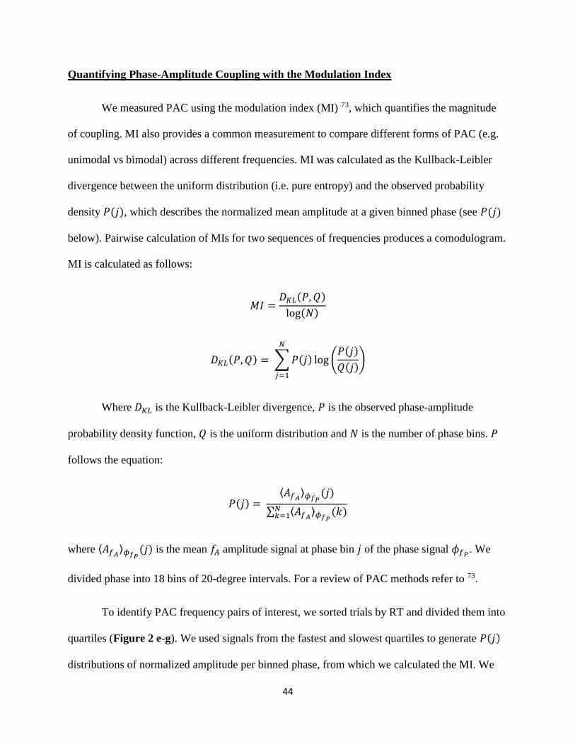
44
Quantifying Phase-Amplitude Coupling with the Modulation Index
We measured PAC using the modulation index (MI) 73, which quantifies the magnitude
of coupling. MI also provides a common measurement to compare different forms of PAC (e.g.
unimodal vs bimodal) across different frequencies. MI was calculated as the Kullback-Leibler
divergence between the uniform distribution (i.e. pure entropy) and the observed probability
density 𝑃(𝑗), which describes the normalized mean amplitude at a given binned phase (see 𝑃(𝑗)
below). Pairwise calculation of MIs for two sequences of frequencies produces a comodulogram.
MI is calculated as follows:
𝑀𝐼 =𝐷𝐾𝐿(𝑃, 𝑄)
log(𝑁)
𝐷𝐾𝐿(𝑃, 𝑄) = ∑ 𝑃(𝑗) log (𝑃(𝑗)
𝑄(𝑗))
𝑁
𝑗=1
Where 𝐷𝐾𝐿 is the Kullback-Leibler divergence, 𝑃 is the observed phase-amplitude
probability density function, 𝑄 is the uniform distribution and 𝑁 is the number of phase bins. 𝑃
follows the equation:
𝑃(𝑗) = ⟨𝐴𝑓𝐴
⟩𝜙𝑓𝑃(𝑗)
∑ ⟨𝐴𝑓𝐴⟩𝜙𝑓𝑃
(𝑘)𝑁𝑘=1
where ⟨𝐴𝑓𝐴⟩𝜙𝑓𝑃
(𝑗) is the mean 𝑓𝐴 amplitude signal at phase bin 𝑗 of the phase signal 𝜙𝑓𝑃. We
divided phase into 18 bins of 20-degree intervals. For a review of PAC methods refer to 73.
To identify PAC frequency pairs of interest, we sorted trials by RT and divided them into
quartiles (Figure 2 e-g). We used signals from the fastest and slowest quartiles to generate 𝑃(𝑗)
distributions of normalized amplitude per binned phase, from which we calculated the MI. We

45
verified the precision of our methods with simulations using methods defined in the appendix of
Tort et al. 73(Supplemental Figure 1 b-f). Specific parameters or MATLAB scripts used for
simulations are available upon request.
Statistical Analysis
Band Limited Power and PAC Time Series Comparisons: Statistical inference testing of
band-limited power and PAC time series followed methods described by Maris and Oostenveld
92. Cluster candidates were generated using t-statistics to test the null hypothesis that there was
no difference between categories at each sample. If a sample t-statistic exceeded an alpha level
of 5% then the null hypothesis was rejected for the sample and it was considered a cluster
candidate. Temporally adjacent cluster candidates were grouped into a single cluster and their t-
statistics were summed to produce a clustering statistic. The clustering statistic of the observed
data was tested against a permutation distribution. To produce the permutation distribution, trial
labels (e.g. valid vs invalid) are shuffled and randomly reassigned 10,000 times. For each
shuffle, cluster candidates and clustering statistics were generated as described above. The
maximum clustering statistic from each shuffle was used to create the permutation distribution.
We calculated p-values for observed clusters using the formula p = (r+1)/(n+1), where r is the
number of shuffled clustering statistics greater than the observed clustering statistic and n is the
total number of shuffled sets used 95. We corrected for multiple comparisons across cortical sites
with the False Discovery Rate (FDR) correction method.
Phase-Amplitude Coupling Comparison: We adapted a two-dimensional non-parametric
permutation test to make cluster-based statistical inferences on comodulograms based on the
difference between fast and slow trials. First, we generated 1,500 shuffled distributions for each

46
cortical site by randomly reassigning RTs to trials, sorting, dividing into quartiles, and
calculating the absolute difference in comodulograms for fast and slow trial quartiles as follows:
𝑑𝑓𝐴𝑓𝑃= |𝑀𝐼𝑓𝐴𝑓𝑃
𝑓𝑎𝑠𝑡− 𝑀𝐼𝑓𝐴𝑓𝑃
𝑠𝑙𝑜𝑤|
We use the pooled variance in each frequency pair in the distribution of 𝑑𝑓𝐴𝑓𝑃
𝑠ℎ𝑢𝑓𝑓𝑙𝑒𝑑 to determine
the cutoff threshold specific to each frequency pair. Adjacent supra-threshold frequency-pairs
were grouped together in clusters and t-statistics were summed. We tested the null hypothesis
that the shuffled data was no different from the observed data using a two-dimensional cluster
based permutation test where diagonals were not considered neighbors 92.
PAC time series were calculated using MI calculations in a 500 ms sliding window with
50 ms increments. While this window only includes half a 1 Hz cycle, we empirically confirmed
that the large amount of data (>250 seconds) used in these analyses ensured that all phases of the
1 Hz cycle were represented in the MI calculation. Differences between PAC time-series for
spatial and behavioral site categories were calculated with the one-dimensional cluster-based
permutation test described above.
Inter-trial coherence and preferred phase statistics: Inter-trial coherence is the
magnitude of the mean phase across trials. It reflects the phase consistency across trials for every
time point and frequency. Preferred phases were calculated as the maximum phase-bin in the
phase-amplitude probability density plot (see 𝑃(𝑗)above). Preferred phases were calculated
separately for each cortical site. The non-uniformity of preferred phases was determined with the
Rayleigh test and the equivalence of the circular means for spatial and behavioral sites was
calculated with the Kuiper test 96.
Sharp Waveform Detection

47
To detect the presence of sharp waves we employed methods from QRS detection in
ECG analyses 97,98. We used the first differential of the ECoG Signal to identify periods of rapid
change. The Hilbert transformation is then applied as an envelope function where peaks
corresponded to locations of candidate sharp wave. We set a threshold of one standard deviation
from the mean. Any candidate sharp wave that did not surpass this threshold for more than 16 ms
was rejected. Finally, we calculated the amplitude change, or height, of each candidate sharp
wave and rejected the bottom 80% to ensure that the most prominent waveforms were being
isolated.
4.4 Results
Figure 4.4.1 Task design showing analysis periods and behavioral results: (A) Subjects
participated in a Posner cued attention task, with the most probably target location
indicated by an arrowhead presented at fixation prior to target onset. Phase-amplitude
coupling (PAC) was analyzed during the cue period. Functional classifications were based
on high-gamma amplitude during the target period. Subjects responded to “L” and “T”
targets with left and right mouse clicks. (B) Reaction times were greater for invalid than
valid trials and (C) for variable than fixed delays.

48
Reaction time reflects task performance
We employed a spatial cueing task to induce and measure covert shifts in spatial
attention. Participants fixated on a central crosshair throughout the task. At the beginning of each
trial a central arrow, or “cue”, pointed towards the most likely location of a subsequent “target”.
Two target locations were possible. We defined these locations as “contralateral” or “ipsilateral”,
depending on whether it was on the same side, or the opposite side, of the recording sites. The
cue predicted the location of the target in 80% of trials (i.e. valid trials). In 20% of trials the
target appeared opposite to where the cue pointed (i.e. invalid trials). In our version of the task
participants were required to discriminate “L” from “T” targets that were randomly rotated
(Figure 4.4.1, top). Across six participants, 5100 of 5344 trials were completed with 92.2%
correct responses. We used trials with correct responses for further analyses. Invalid trials
incurred higher RTs than valid trials (medians (ms): valid = 831, invalid = 927, rank sum: 7.2e6,
approximate z-value: -9.8, p = 1.6e-22). No differences in reaction time occurred between trials
with contralateral and ipsilateral cues (medians (ms): contralateral=860, ipsilateral=863, rank
sum: 5.1e6, approximate z-value: -1.7, p=0.08). Higher RTs on invalid trials confirmed that the
task induced lateralized shifts in visual attention.

49
We focused our physiological analyses on two periods in the task, the “cue period” and
the “target period”. We define the “cue period” as the time between cue onset and target onset
and the “target period” as the first 400ms after target onset. Cued shifts in attention occurred
during the cue period. The target location and identity is revealed during the target period,
allowing subjects to locate the target, identify it, and subsequently respond appropriately.
Figure 4.4.2 Identification of distinct phase-amplitude coupling clusters: (A-B) Single trial
examples of more coupling on fast trials than slow trials (A) Beta (25 Hz) amplitude

50
couples to alpha phase (8 Hz) and (B) gamma (70 Hz) amplitude couples to delta (1 Hz)
phase. High-frequency amplitude envelopes are colored with low-frequency phase. (C)
Mean beta amplitude at binned alpha phase and (D) mean gamma amplitude at binned
delta phase. € Mean modulation indices calculated for pairwise frequencies. (F) T-statistics
from permutation distributions were used to determine significance. (G) Delta-high gamma
(DH, yellow), theta/alpha-beta/low gamma (TABL, red) and theta/alpha-high gamma
(orange) clusters, calculated during the cue period predicted reaction time.
Distinct clusters of PAC predict RT:
We identified behaviorally relevant PAC frequencies by comparing the cue periods
preceding fast and slow RTs. After sorting trials by RT, we binned them into quartiles and
analyzed differences in cue period PAC between the fastest and slowest quartiles. We found
PAC differences in multiple frequency pairs (Figure 4.4.2a, b). For visualization purposes,
color-coded low-frequency phases are projected on the high-frequency amplitude envelope (for
reference see Supplemental Figure 1 b, d). The modulation index (MI) quantified PAC
intensity, or the non-uniformity of the phase-amplitude probability density plot (Figure 4.4.2c,
d). We calculate the MI for each frequency pair to generate a comodulogram. The absolute
difference between slow and fast comodulograms averaged over all cortical sites and subjects,
revealed coupling between delta-phase and theta-alpha-phase to higher frequency (>20Hz)
amplitude envelopes (Figure 4.4.2e).
Cluster-based permutation testing determined the significance of PAC while controlling
for false positives. Permutation distributions were generated by shuffling reaction times between
trials and calculating absolute differences in comodulograms between the slowest and fastest
quartiles in shuffled datasets. Significant phase-amplitude frequency clusters outlined adjacent

51
frequency pairs with significant t-statistics (Figure 4.4.2f). Three clusters of frequency pairings
explained RT variance: 1) theta-alpha-phase/beta-low gamma-amplitude (TABL) (Figure 4.4.2g,
red), 2) delta-phase/high-gamma-amplitude (DH) (Figure 4.4.2g, yellow), and 3) alpha-
phase/high-gamma-amplitude (Figure 4.4.2g, orange). We focused on comparing DH with
TABL PAC for three reasons. First, they have unique phase and amplitude frequencies, unlike
alpha-high gamma PAC. Second, the magnitudes of DH and TABL PAC were the least
correlated across all electrodes. Third, TABL and DH PAC have been shown to underlie distinct
mechanisms in human memory 69. Therefore, we hypothesized that DH and TABL were most
likely to show different functional characteristics during the spatial attention task.
To verify precision in measuring frequency-specific PAC we modeled PAC with
simulated signals using procedures from Tort and colleagues 73 (Supplemental Figure 1 a-e).
We inspected subject-specific differences in PAC by inspecting averaged comodulograms
alongside electrode locations on an averaged brain plots. Five of six subjects displayed robust
TABL PAC. Most subjects had less DH PAC magnitude compared to TABL PAC
(Supplemental Figure 3). Interestingly, TABL PAC did not appear on single trials and only
emerged when we calculated phase-amplitude distributions on multiple (>15) trials
(Supplemental Figure 2). To explore differences in TABL and DH PAC we returned to
disparities in the motivating literature. While both Esghaei et al. and Szczepanski et al. found
that PAC depended on spatial task variables, only the latter found that PAC correlated with RT
48,75. Therefore, we explored whether DH and TABL PAC uniquely depended on spatial
variables or task performance (i.e. RT) by classifying cortical sites by function and comparing
PAC across functional classes.

52
Figure 4.4.3: Functional classification of “spatial and “behavioral” cortical sites. Spatial
cortical sites have high gamma (75-150 Hz) activity that discriminates spatial parameters of
the task. Exemplary mean high gamma power, with standard error bars, from two spatial
cortical sites discriminating (A) valide from invalid targets and (C) targets that appear
contralateral from targets that appear ipsilateral to recording sites. (B) Distribution of
spatial cortical sites where red dots discriminate validity and blue dots discriminate
location. Behavioral cortical sites had high gamma activity that correlated with reaction
times (RTs). (D) exemplary correlation from one behavioral cortical site. (E) The cortical
surface distribution of behavioral sites. (F) Breakdown of electrode classifications for each
participant (left vertical axis) and for all participants (right vertical axis)

53
Functional classification of spatial and behavioral cortical sites:
We classified cortical sites based on high-gamma (75-150 Hz) power as it has been
shown to correlate with local neuronal activity 99. We classified neural activity in the target
period for two reasons. First, this period had the most robust discriminatory neural responses.
Second, all the information required for a correct response was made available in the target
period. Therefore, all classifications relied on high-gamma power in the first 400 milliseconds
after target onset.
We defined "spatial" cortical sites based on neural activity discriminating target location
or validity. Due to the contralateral organization of visual receptive fields, contralateral targets
typically produced larger neural responses than ipsilateral targets. Invalid targets, occurring on
20% of trials, typically produced larger changes in high-gamma power than valid targets. We
justified grouping validity sensitive sites with location sensitive sites because calculating a
target’s validity requires the target’s location as an operand. Thus, we classified a cortical site as
“spatial” when its high-gamma power discriminated either contralateral from ipsilateral targets
(Figure 4.4.3a) or valid from invalid targets (Figure 4.4.3c, cluster permutation test threshold p
< 0.05, FDR corrected). In contrast, we defined “behavioral” cortical sites based on
discriminatory neural activity pertaining to RT. Behavioral cortical sites had significant
Spearman correlations between mean post-target high-gamma power and RT (Spearman
correlation threshold p < 0.05, FDR corrected). Mean high-gamma and RT had log-normal
distributions so we represent this as a correlation of the log of both values in Figure 4.4.3d.
Spurious correlations were ruled out with a permutation test using 5000 identical correlations
with shuffled RTs.

54
We found 51 spatial and 127 behavioral sites. We removed the 13 sites classified to both
groups and 237 classified to neither group, from further analyses (Figure 4.4.3f). Spatial cortical
sites were found primarily over visual cortex, parietal cortex, motor cortex and frontal cortex,
with the distribution of dorsal parietal and posterior frontal sites roughly matching the dorsal
attention network 11 (Figure 4.4.3b). Behavioral cortical sites were found over motor cortex,
parietal cortex, and temporal cortex (Figure 4.4.3e). We compared these two functional classes
to investigate functional properties of TABL and DH PAC.
Figure 4.4.4 Phase preferences and relative PAC magnitude distinguish coupling
frequencies and functional classes. (A) Preferred phases differed for delta to high-gamma
(DH) PAC (top row) and theta-alpha to beta-low-gamma TABL PAC (bottom row) across
spatial (left column) and behavioral (right column) cortical sites. Coupling emerged in the
cue period (blue) relative to baseline pseudo-trials (red). Arrows indicate the circular mean
of preferred phases across all subjects and cortical sites. (B) The relationship between PAC
magnitude (left column) and the corresponding frequency-for-amplitude power (right
column) reverses across behavioral (red) and spatial (blue) cortical sites. Solid black lines

55
at top of graph indicates clusters of samples where spatial and behavioral signals were
significantly different at p<0.05.
Phase and magnitude differentiate PAC clusters across functional classes:
We first characterized differences in the phase preferences and coupling magnitudes of
DH and TABL PAC. We defined preferred phases as the low-frequency phase bin with the
greatest high-frequency amplitude. Preferred phases are independent of coupling magnitude, and
if no coupling exists then preferred phases will be uniformly distributed on average. We
calculated the preferred phase using all cue periods, then calculated the circular mean across all
cortical sites within a functional class. We repeated this analysis for pseudo-trials generated from
the rest period recorded prior to the task to ensure that coupling did not exist during rest. Pseudo-
trials had identical length to the cue period, but were sampled randomly from the rest period.
During rest, preferred phases were uniformly distributed in both functional classes and
frequency pairs (Rayleigh test, TABL PAC: spatial z = 1.5, p = 0.86; behavioral z = 0.97, p =
0.38; DH PAC: spatial z = 0.03, p = 0.97; behavioral z = 2.86, p = 0.06; Figure 4.4.4A, red). In
contrast, all sites had preferred phases during the cue period. (Rayleigh test, TABL PAC: spatial
z = 28, p = 1e-12; behavioral z = 41, p = 6e-20; DH PAC: spatial z = 37, p = 3e-9; behavioral z =
71, p = 4e-32, Figure 4.4.4A, blue). Furthermore, the mean DH PAC phase preferences differed
across spatial and behavioral sites (spatial mean=237, std=67, behavioral mean=321, std=69,
Kuiper test, k = 1.1e5, p = 0.001, Figure 4.4.4A top). However, TABL PAC consistently
showed a 180-degree phase preference in all sites (spatial mean=184, std=42, behavioral

56
mean=178, std=53; Kuiper test, k = 1.7e4, p = 0.10, Figure 4.4.4A bottom). Phase preferences
were not affected by cue direction or reaction time. Therefore, the preferred phases of DH and
TABL PAC during the cue period showed consistent differences.
We hypothesized that spatial sites were more active than behavioral sites during the cue
period. To verify this, we compared high-gamma variance and inter-trial coherence (ITC) across
functional classes. High-gamma power and variance were greater in spatial sites than in
behavioral sites (power: cluster permutation test p<0.001 Figure 4.4.4B, top right, variance:
rank sum, p<0.001 Supplementary Figure 4A). ITC measures the coherence over trials in both
phase and amplitude. Again, spatial sites had greater ITC in the 1-10 Hz frequency range during
the cue period (Supplemental Figure 4B, C). Taken together, neural activity in spatial sites
were more modulated by spatial cueing than behavioral sites were in both low and high
frequencies. DH PAC paralleled these indexes of neural modulation and was higher in spatial
sites than in behavioral sites (cluster permutation test, p < 0.001, Figure 4.4.4B top left).
Furthermore, DH PAC peaked after cue onset and target onset, much like high gamma power. In
contrast, TABL PAC was greater in behavioral sites than in spatial sites (cluster permutation test,
p < 0.001, Figure 4.4.4B bottom left). This was not due to high beta or low-gamma power, both
of which were greater in spatial sites (cluster permutation test, p <0.001, Figure 4.4.4B bottom
right). It was also not due to greater alpha activity in behavioral sites (Supplemental Figure
4E). Finally, this was not due to baseline differences as there were no significant differences in
beta, low-gamma or alpha power at rest across the functional classes. Therefore, high TABL
PAC corresponded to reduced neural modulation across the functional categories.
To summarize, TABL PAC and DH PAC showed a reversal in their relationship to
power. TABL PAC was greater in behavioral sites, despite reduced power, variance and ITC. In

57
contrast, DH PAC positively co-varied with every measure of neural modulation we measured.
Since there were no observed differences in PAC or power at baseline, this reversal was best
explained by the task. Along with differences in phase preference, magnitude differences
provided additional evidence that DH and TABL PAC dynamics depended on functional
classifications.
Figure 4.4.5 PAC magnitude differences across task conditions distinguish between phase
frequencies and functional classes. (A) Shows positive comodulogram differences for
behavioral (left) and spatial (Right) sites when subtracting contralateral from ipsilateral
trials (top) and fast from slow trials (bottom). These changes were quantified using
previously identified PAC clusters. (B) No ipsi-contra differences were observed as a
product of lateralized cued attention in theta/alpha-beta/low gamma (TABL) PAC at either

58
spatial or behavioral sites. (C) Delta-high gamma (DH) PAC increases on contralateral vs
ipsilateral trials in spatial sites relative to behavioral sites. (D) Table PAC was more
negatively correlated with RT in behavioral than spatial sites. DH PAC showed no
differences between behavioral and spatial sites (E).
Distinct PAC frequency pairs correspond to cortical function
We investigated PAC differences across spatial conditions (i.e. contralateral vs ipsilateral
cues) and behavioral responses (i.e. RT) (Figure 4.4.5A). We quantified differences using
previously defined clusters (Figure 4.4.2G). On contralateral trials, we found increased DH PAC
in spatial cortical sites and no change in behavioral sites (sign test, spatial: z-value 2.6, p = 0.009,
behavioral: z-value = -1.8, p = 0.07; Figure 4.4.5C). The difference between classes was
significant (rank sum, z-value = -3.4, p = 7e-4, corrected). TABL PAC showed no changes
across ipsilateral and contralateral cueing conditions and there were no differences between
classes (sign test, spatial: z-value 1.05, p = 0.29, behavioral: z-value = 0.94, p = 0.34, rank sum,
z-value = 0.15, p = 0.9, Figure 4.4.5B). This suggested DH PAC was specific to spatial variables
in spatial sites.
To understand which functional class drove differences between fast and slow trials we
correlated DH and TABLPAC with RT for all sites in each functional class. Spatial sites showed
no significant trend in correlations (t-test, DH vs RT ≠ 0: p = 0.80, TABL vs RT ≠0: p = 0.97)
and there were no differences between Fisher transformed r-value distributions (t-test, DH vs RT
≠ TABL vs RT: p=0.90, Figure 4.4.5E). In contrast, TABL PAC was more negatively correlated
with RT in behavioral sites (t-test, DH vs RT ≠ TABL vs RT: p<1e-11, Figure 4.4.5D). To

59
summarize, during the cue period DH PAC in spatial sites varied with cue direction and TABL
PAC in behavioral sites correlated with RT.
Figure 4.4.6: Transient waves are behaviorally relevant and coupled to 7.2 Hz phase. (A)
Raw ECoG signal shows three sharp waves that correspond to (B) theta (6 Hz)-phase, beta
(25 Hz)-amplitude coupling with a 180-degree phase preference. (C) Hilbert transform of
the differential of the raw ECoG signal amplifies rapid (i.e. sharp) changes in the ECoG
signal. A threshold on the Hilbert-Differential identified the transient waves. (D) Single
trials sorted by RT and grouped into 30-trial bins with median RTs below each column.
Red circles highlight identified sharp waves that were more likely to occur on trials with

60
fast reaction times. € Correlation between the number of sharp waves in an RT-bin and
RT. (F) the averaged waveform for the cortical site in (D) and (E). (H) the distribution of
correlation coefficients for spatial and behavioral sites. (I) distribution of inter-sharp wave
intervals peak at 138 ms, corresponding to 7.2 Hz.
Coupled sharp waves correspond to TABL PAC:
DH PAC has been described in prior attention literature 45,48,75, but TABL PAC has not
been previously shown in attention tasks. It has, however, been shown to correlate with encoding
and retrieval in memory tasks 69. Additionally, non-sinusoidal or “sharp” waveforms have been
shown to produce coupling in the TABL PAC frequency range 69,86. We hypothesized that if
sharp waveforms resulted in TABL PAC, then they too will correlate with RT. Furthermore, we
hypothesized that, compared to computationally expensive PAC analyses, more efficient
methods could be used to detect and characterize sharp waveforms.
On visual inspection of the raw ECoG we found that transient waveforms temporally co-
occurred with TABL PAC (Figure 4.4.6A, B). We reasoned that the “sharpness” of the wave
could be used to detect these events and employed techniques previously used for QRS wave
detection in electrocardiogram analyses 97,98. This method uses the Hilbert transform of the
differential to identify rapid (i.e. sharp) changes in the raw signal (Figure 4.4.6C). We applied
this sharp wave detection to individual trials and displayed the results in 30-trial RT bins (Figure
4.4.6D). We found that trials with fast responses (i.e. low RTs) were more likely to have sharp
waveforms than slower trials (Figure 4.4.6E). In aggregate, sharp waveform correlations with
RT were significantly more negative in behavioral sites than in spatial sites (rank sum p<0.001,

61
Figure 4.4.6H), similarly to TABL PAC (Figure 4.4.5D). Alongside the correlations for specific
channels we used the minimum of the detected sharp wave to time-lock waveforms and observe
their shapes. We observed that detected sharp waves consisted of a roughly 50 ms transient
wave (Figure 4.4.6F).
Finally, it remained unclear whether these sharp waves were themselves coupled to a low
frequency rhythm, so we analyzed the intervals between sharp waves. For every trial with more
than one sharp wave we recorded the interval between adjacent sharp waves. The distribution of
inter-sharp-wave intervals was not log-normal or Poisson (chi-square goodness-of-fit both
p<0.0001), which would be expected if intervals were randomly spaced. Instead, a peak of 138
ms suggested that sharp waves coupled to a 7.2 Hz oscillation (Figure 4.4.6I).
In summary, TABL PAC associated with sharp waveforms that could be detected with
time-domain methods. However, the distribution of sharp wave intervals suggested that they
occur regularly within a theta-alpha range oscillation. Therefore, sharp wave morphometry and
the frequency of sharp waveform events contributes to TABL PAC. While characterization of
these transient waveforms may require nuance, their correlations with RT across functional
classes matched that of TABL PAC, suggesting a common origin.
4.5 Discussion
This study expands our understanding of phase amplitude coupling (PAC) in several
ways. First, we identified an interaction between theta-alpha-phase and beta-low-gamma
amplitude (TABL PAC) during spatial cueing that predicted future reaction times (RTs) and is
novel to the attention literature. Second, we characterized differences between TABL PAC and
delta-phase, high-gamma-amplitude coupling (DH) PAC. Specifically, we found DH PAC

62
positively covaried with contralaterally cued attention in spatial sites while TABL PAC
correlated with RT in behavioral sites. Unlike DH PAC, TABL PAC negatively covaried with
multiple indices of neural modulation and maintained a consistent 180-degree preferred phase
during the task. Third, we identified sharp wave correlates of TABL PAC using novel and
efficient methods, which showed that sharp waveforms predict RT. Finally, we showed that
behaviorally relevant sharp waveforms are also coupled with low frequency oscillations. Taken
together, this study highlights the unique contributions of distinct PAC frequency clusters in a
spatial attention task.
Methodological considerations for frequency-specificity in PAC analysis:
The complexity of PAC analyses 74, evidence for spurious PAC 87,100, and the novelty of
TABL PAC in spatial attention tasks warrants a discussion of methods. We employed the
modulation index (MI) to measure the intensity of PAC due to its advantages over other methods
(for a review, see Tort et al., 2010). Sufficient data length was critical to resolving TABL PAC.
This was due to the relative sparsity of transient waveforms leading to TABL PAC on single
trials. Additionally, coupling between two frequencies (e.g. Fp and Fa) can only occur in the
presence of two additional frequencies: the sum and the difference of the original two
frequencies (i.e Fa+Fp and Fa-Fp, see Supplemental Figure 1A arrows). To account for this,
we developed wavelet libraries independently for phase and amplitude signals. Wide band-width
amplitude filters were required to measure PAC in higher phases 74,101. Conversely, narrow band-
widths allowed phase-specificity when filtering phase signals, since broadband phase estimates
may include separable PAC components that cancel each other out.
In addition to signal processing and measurement considerations, we used reaction time
to identify behaviorally relevant PAC frequency clusters. Furthermore, instead of shuffling

63
phase and amplitude signals relative to each other, we shuffled trials between behavioral
categories (e.g. fast and slow RT quartiles) to generate chance distributions. This guaranteed that
our statistical inferences were made from distributions with physiologically observed phase-
amplitude relationships. We then employed a non-parametric cluster-based permutation test for
statistical inferences. These methods resolved behaviorally relevant PAC frequency clusters
spanning frequency bands previously associated with attentional processes 42,44,46,67
Sharp Waveforms are Dynamically Coupled
We propose that sharp waveforms are a behaviorally relevant, special case of PAC. This
is an alternative to suggestions that non-sinusoidal sharp waveforms are spurious 86,102. We
demonstrated transient beta (50 ms) waves that occurred at 138 ms intervals, suggesting a
coupled dynamical process. Similar waveforms have been shown across species 103 and have
relevance to human memory tasks 69. Sharp waveforms have high frequency components
coupled to the phase of low frequency rhythms, which is fits the definition of PAC. In the
context of dynamic brain activity, persistent nesting of sinusoidal oscillations is another special
case of PAC, not the only possibility. PAC approaches identify frequency interactions between
high and low frequencies that can lead to a better understanding of underlying dynamics.
Because PAC analyses are computationally expensive and sensitive to noise, we used our PAC
approach to inform a computationally inexpensive approach, which better described individual
trials.
A theoretical framework and implications for PAC in attention
Two hypotheses are relevant to PAC and cued spatial attention (for an extensive review
see 83. The communication through coherence (CTC) hypothesis proposes that excitability

64
windows of two communicating brain regions are temporally aligned by low frequency
oscillations to promote information transfer (e.g. spikes) across regions 104,105. In contrast, the
gating by inhibition (GBI) hypothesis proposes that low frequencies periodically suppress
information in a neuronal population 106.
Although we do not have evidence to assess the CTC hypothesis, we found evidence for a
suppressive role for TABL PAC, which fits with the GBI hypothesis. First, multiple indices of
neural modulation suggested spatial sites were more active than behavioral sites during spatial
cueing, yet TABL PAC was greater in behavioral than spatial sites. Furthermore, TABL PAC
consistently demonstrated a 180-degree phase preference, which meant that high frequency
activity preferred the trough of the low frequency oscillation. This pattern of coupling has been
shown in “pulsed-inhibition” or “gating by inhibition” models of alpha oscillatory activity 47,106,
where the peak of alpha oscillatory amplitude periodically suppresses higher frequency activity.
Finally, the transient waves that cause TABL PAC have been shown in multiple species and
studies to relate to decreased information relay 103,107. Taken together these results support a
suppressive function of TABL PAC during our spatial attention task.
Conclusions
Spatial attention enhances neural responses to attended stimuli and by filtering out
unwanted information 108. Prior studies differed on whether PAC contributes to selection 48 or
filtering 75. Here we show evidence that the functional properties of PAC depend critically on
phase frequency. DH PAC facilitates lateralized spatial attention while TABL PAC contributes
to behavioral performance, potentially through suppressive gating of activity. Furthermore, we
demonstrate that sharp waves producing TABL PAC are themselves coupled to low frequency

65
oscillations. While the function of these sharp waves remains unclear, PAC remains a useful tool
in understanding the neural correlates of human attention.
4.6 Supplemental Figures:

66

67
Figure 4.6.1 Supplemental figures

68
5) Alpha-phase Coupling Distinguishes Mechanistically
Distinct Unconscious States
5.1 Introduction Coupling of neural oscillations has been shown to correlate with cognition and behavior
in multiple species, using multiple modalities 48,75,81,109,110. One form of coupling called phase-
amplitude coupling (PAC) has been proposed a fundamental mechanism for controlling cortical
communication 83,85. However, this idea has been challenged by examples of spurious PAC 87,100
and violations to the mathematical constraints of PAC analyses 74,101. In this study, we exploit the
cognitive differences between conscious and unconscious states to study the role of PAC.
Specifically, we investigate PAC changes caused by slow wave sleep (SWS) and Propofol-
induced loss of consciousness (PLOC). The gating by inhibition (GBI) hypothesis is particularly
relevant to loss-of-consciousness because it suggests that low-frequencies periodically suppress
transmission of neural information 83. This hypothesis is relevant because SWS has been shown
to suppress cortical transmission 54 and Propofol causes inhibition through GABA-A agonism
111. Prior studies have explored changes in PAC during SWS 57,112–114, changes in PAC during
Propofol anesthesia 115,116, and differences in SWS and Propofol anesthesia with scalp EEG 62.
However, no study to date has compared differences in PAC across these two distinct forms of
loss-of-consciousness using invasive electrophysiology in humans.
Sleep is organized by the interplay of suprachiasmatic nucleus cells and a complex set of
regional networks in the hypothalamus 117. It has been shown in human TMS studies that cortical
excitability is diminished during sleep 54. Despite this, sleep is not a passive brain state, but an

69
active process at both subcortical and cortical levels 118. Accordingly, many electrophysiological
features can be measured at the scalp during sleep. These features include slow waves, sleep
spindles and k-complexes, each with a well-studied circuitry 119,120. In a recent invasive
electrophysiological sleep study, PAC was greater during SWS, when compared to wake, for
delta-, theta- and alpha-phases coupled to 30-260 Hz amplitude 112. This result conflicts with
evidence that increased PAC facilitates attention 48,81, since attention is markedly reduced during
SWS 58. More specifically, alpha-phase has a prominent role alertness 121,122 , perception 47, and
selective attention, 123 presumably through an inhibitory mechanism 19,106. These findings are
difficult to reconcile with increased alpha-phase PAC during SWS. For these reasons, we
hypothesized that alpha-phase PAC scales with inhibitory attention mechanisms and decreases
during SWS.
PLOC shares several physiological similarities with sleep. For example, sleep debt, the
cumulative requirement for sleep caused by sleep deprivation, facilitates Propofol induction and
Propofol anesthesia relieves sleep debt 59,60. Furthermore, slow waves are present in both SWS
and PLOC recordings 124. Despite these similarities, it is considerably more difficult to arouse
someone from PLOC, compared to SWS. Additional electrophysiological differences include the
failure of Propofol-induced slow waves to entrain high frequency activity and an anteriorization
of alpha activity that occurs in Propofol anesthesia 62,64. PLOC has an inhibitory mechanism of
action through GABA-A agonism 111,125. In contrast, evidence suggests that reduced excitability
during SWS is due to disfacilitation caused by potassium leak currents rather than GABA-A
mediated inhibitory postsynaptic potentials 126. Comparing PAC between SWS and PLOC
provide a unique window into the role of PAC in the brain.

70
In this study, we measure PAC in 10 subjects with invasively monitored
electrocorticography. Four subjects were monitored during sleep and awake states, five subjects
were monitored during anesthetic induction using Propofol and one subject was monitored in
both conditions. We hypothesized that alpha-phase coupling indexes inhibitory gating and would
therefore discriminate the mechanistic differences between PLOC and SWS. We measure PAC
in both conscious and unconscious states using the modulation index described by Tort et al. 73.
In contrast to prior studies 112, we found a double dissociation between sleep state and phase-
frequency. Delta-phase coupling increased, but alpha-phase coupling decreased during SWS
compared to wakefulness. [We confirmed this finding in an open EEG sleep dataset with 29
subjects.] Importantly, we found that this double dissociation did not occur during PLOC. PAC
involving theta- and alpha-phase increased during PLOC compared to wakefulness. We conclude
that coupling to alpha-phase distinguishes SWS from PLOC and that this increased alpha-PAC
may indicates Propofol-induced cortical inhibition.
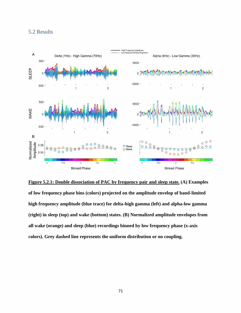
71
5.2 Results
Figure 5.2.1: Double dissociation of PAC by frequency pair and sleep state. (A) Examples
of low frequency phase bins (colors) projected on the amplitude envelop of band-limited
high frequency amplitude (blue trace) for delta-high gamma (left) and alpha-low gamma
(right) in sleep (top) and wake (bottom) states. (B) Normalized amplitude envelopes from
all wake (orange) and sleep (blue) recordings binned by low frequency phase (x-axis
colors). Grey dashed line represents the uniform distribution or no coupling.

72
Double dissociation of delta-phase and alpha-phase PAC across wake and sleep states:
We evaluated the difference in PAC between slow wave sleep (SWS) and wake. Figure
5.2.1 demonstrates exemplar coupling patterns elucidating differences between SWS and
wakefulness in alpha- and delta-phase PAC. Delta-high gamma (1 Hz – 70 Hz) PAC was greater
during sleep (Figure 5.2.1A top left) than during wakefulness (Figure 5.2.1A bottom left). For
visualization purposes, we color-coded the phase of the lower frequency (i.e. 1 Hz) on the
amplitude envelope of high-gamma. If the high frequency amplitude was consistently higher on a
particular phase of the low frequency signal, coupling existed. The magnitude of delta-high
gamma coupling is quantified by the modulation index, or the non-uniformity in the phase-
amplitude probability density plot (Figure 5.2.1e). Differences in delta-high gamma coupling
can be observed between sleep and wakefulness (Figure 5.2.1A left). This is difference is
quantified in the phase-amplitude probability density (Figure 5.2.1f, red vs blue).
Alpha-phase PAC had the opposite relationship to SWS. We found an absence of alpha-
low-gamma (9Hz – 30Hz) coupling during SWS (Figure 5.2.1b) and higher coupling during
wakefulness (Figure 5.2.1d). This difference is quantified on the phase-amplitude plot (Figure
5.2.1f, red vs blue). To evaluate the generality of this double dissociation we tested for
differences in wake-SWS comodulograms using a cluster-based permutation method and found
significant increases in delta-broadband PAC, along with significant decreases in alpha-
broadband PAC, during SWS (both p<0.001. see Supplementary Figure 5.2.1).

73
Figure 5.2.2: TABL PAC decreases during SWS but increases during PLOC. (Top) The
difference in Wake – SWS comodulograms reveals more TABL PAC in waking state
(orange). (Bottom) The difference in Wake – PLOC shows the opposite, a higher TABL
PAC in PLOC.
Increase in theta/alpha PAC marks propofol LOC
In stark contrast to SWS, PAC increased dramatically during PLOC and the aggregate
change in PAC across cortical sites was consistent. In the transition from wakefulness to SWS
there is an increase in delta-phase PAC, no change in theta-phase PAC and a reduction in alpha-
phase PAC (Fig 3A). In contrast, propofol induction showed a generalized increase in PAC.
Delta-, theta- and alpha-phase PAC significantly increased in the last minute of induction,
compared to the first (Fig 3B). Furthermore, while the increase in delta-phase PAC in both SWS

74
and LOC were accompanied by an increase in power, this was not the case for theta and alpha.
Median band limited power using Welch’s method demonstrated no change in theta and alpha
power in both forms of LOC (Fig 3 C, D, blue highlight).
In summary, we have shown that the marked reduction in alpha-phase PAC that occurs in
the transition from waking to SWS does not occur in propofol induction. In fact, we see a
significant increase in alpha-phase coupling. This increase in coupling cannot be explained by
changes in alpha power. Furthermore, we found a larger reduction in beta, low gamma and high
gamma in propofol induction, compared to SWS. Therefore, the increase in theta- and alpha-
phase coupling is most likely due to the timing of high-frequency bursts of activity (i.e. >25 Hz)
relative to the phase of low frequency (i.e. theta and alpha) phase. It is also notable that a)
theories on alpha’s role in cognition and b) propofol’s mechanism of action, both involve cortical
inhibition.

75
A) SWS Change in PAC B) Propofol Change in PAC
C) Sleep Change in Power D) Propofol Change in Power
Figure 5.2.3 Increased theta- and alpha-phase PAC is not caused by changes in power. (A)
Shows the change in PAC from wake (left boxplots) to SWS (right boxplots). The left two
boxes show a positive change in delta-broadband PAC, the middle two boxes display no
change in theta-broadband PAC and the right two boxes show a negative change in alpha-
broadband PAC. (B) Shows the analogous plot to (A) but for the changes in PAC from
wake (left boxplots) to Propofol-induced loss of consciousness (PLOC, right boxplots). We
see that delta-, theta- and alpha-broadband PAC increases. (C,D) The corresponding

76
changes in band-limited power show that delta power increases when transitioning from
wakefulness to both SWS and PLOC. Beta, low gamma and high gamma power decrease in
both SWS and PLOC, compared to waking. However, theta and alpha power does not
change (blue shading).
5.3 Discussion In this study we investigated whether PAC increases or decreases in two states of reduced
arousal SWS and PLOC. First, we identified a double dissociation in PAC frequency pairs and
sleep state. During SWS delta-broadband PAC increased but alpha-broadband PAC decreased. In
contrast, alpha-broadband PAC increased in PLOC, compared to wake. Therefore, the
similarities between SWS and PLOC may be indexed by delta-broadband PAC increases. These
include the ability of both SWS and PLOC to relieve sleep debt. The differences between SWS
and PLOC may be represented in alpha-broadband PAC. The major difference is the mechanism
behind both states. While SWS is related to disfacilitation, PLOC is caused by inhibition.
The differences in the results of our study and the most comparable work in the
literature127 warrants a discussion of methods. In a personal communication with Amiri et. al.,
we learned that the authors did not adhere to the mathetmatical constraints of PAC analyses laid
out in prior theoretical literature74,128. Namely, frequency-for-amplitude filters must have twice
the bandwidth of the frequency-for-phase of interest. If we want to assess coupling to 8 Hz
phase, our amplitude filters must have a 16 Hz bandwidth. Given that Aru et. al. used filters with
insufficient bandwidth, it is likely that their results only reflected delta-broadband coupling. Like
Amiri et. al., out study also demonstrated increased delta-broadband PAC during in SWS. Our

77
additional finding regarding PLOC adds to the understanding of how consciousness and PAC are
related.
Delta-broadband PAC likely represents the slow waves that are common to both PLOC
and SWS. These slow waves may function to periodically disfacilitate neuronal firing. This type
of globally disfacilitated activity may be a marker of low arousal states. On the other hand,
alpha-broadband PAC may specifically represent inhibition. Prior studies have established that
SWS is not an inhibitory state126. In contrast, PLOC has a clear inhibitory mechanism of action,
GABA-A agonism. Taken together, delta-broadband and alpha-broadband PAC can discriminate
waking, SWS and PLOC states along the axes of arousal and inhibition. This new correlate of
conscious state may appear perplexing. Why should waking be more similar to PLOC than SWS
along any axis when behaviorally PLOC and SWS are quite similar? While this topic is beyond
the scope of this research we offer one clinical paradox that may be elucidated by this finding.
Little is known about recovering consciousness in patients that are in vegetative or
minimally conscious states. However, evidence exists that Zolpidem (i.e. Ambien), a GABA-A
agonist like Propofol, can transiently recover consciousness in these patients50. Prior research in
attention suggested that TABL PAC correlates with inhibition (see Chapter 4). Considering the
plethora of information our brains process every moment, we propose the following hypothesis
for why GABA-A agonists may clinically improve consciousness. An inability to sift through the
plethora of information our brain receives may result in an inability to engage in goal-directed
behaviors. Inhibition through GABA-A agonism may temper the onslaught of information just
enough for productive trains-of-thought to be selected and acted upon. Non-invasive
measurements of TABL PAC before and after Zolpidem treatment in vegetative patients may
quantify this change in future experiments.

78
5.4 Supplemental Data
Figure 5.4.1: Consistency of double dissociation across patients. (Top) ECoG grid
placements for all subjects. (2nd Row) Wake - Sleep Comodulograms. (3rd row) T-statistics
for Wake – Sleep across all recording sites. (Bottom Row) Cluster-based permutation
testing reveals significant clusters (red, grey, teal and blue). Frequency-for-amplitude on y-
axis and frequency-for-phase on the x-axis for bottom 3 rows.
Consistent dissociation by phase-frequency and sleep state across subjects:
Comodulograms represent the difference in coupling (i.e. non-uniformity of phase-
amplitude plots), across waking and SWS states (i.e. wake – sleep), for every pair of frequencies
under investigation. We averaged these comodulograms across all cortical sites both within and
across subjects. The five subjects providing sleep and wake data had ECoG grids placed over or
near the Sylvian fissure, with coverage over parts of the temporal, pre-motor, motor, and sensory

79
cortices. ECoG strips were also placed over parieto-occipital regions and ventral regions
(Supplemental Figure 5.4.1a-e, top row). To compare SWS and wake states, we observed the
difference in comodulograms (Supplemental Figure 5.4.1a-e, middle top row), the t-statistics
(Supplemental Figure 5.4.1a-e, middle bottom row) and the cluster-based statistical inference
(Supplemental Figure 5.4.1a-e, bottom row) for each subject 92. All subjects displayed an
increase in delta-phase PAC in SWS compared to wake. Conversely, alpha-broadband PAC was
decreased in SWS, compared to wake. The t-statistic tested the hypothesis that there was no
difference between wake and SWS states and uses the pooled standard error across wake and
SWS for every frequency-pair in the comodulogram. The t-statistics partly rectify the 1/f power-
law distribution and were more sensitive to small, yet stable, differences in PAC at higher phase
frequencies (Supplemental Figure 5.4.1a-e, middle bottom row). When we combined the data
from all subjects, we observed the same dissociation between delta-broadband and alpha-
broadband PAC across wake and SWS (Supplemental Figure 5.4.1f, middle rows).
We used a cluster-based permutation test to assess the significance of these differences.
Adjacent t-statistics above or below a two-tailed threshold (alpha = 97.5) were summed to
generate cluster-statistics. Cluster-statistics were tested against a permutation distribution.
Permutation distributions were created by shuffling wake and SWS labels 1000 times and
repeating the procedure for each shuffle. Only the maximum cluster-statistic was used in the
creation of the permutation distribution. In four of five subjects, a significant cluster associated
with delta-phase emerged distinctly from a significant cluster associated with alpha-phase. The
border between these clusters ranged from 2-7 Hz and both clusters included the entirety of the
frequency-for-amplitude spectrum (20-150 Hz). In the fifth subject (i.e. 148), there was no alpha-
phase cluster. Only one cluster was found that ranged the entire phase and amplitude spectrum.

80
However, this subject had a notable region of non-significance in the theta-alpha-phase (5-15
Hz), beta-low-gamma-amplitude (20-45 Hz) region of the comodulogram. All clusters passed a
threshold of p<0.05, correcting for comparisons using the false discovery rate (FDR) correction
for multiple comparisons (Supplemental Figure 5.4.1a-e bottom row).
We pooled the data from all participants to perform a group-level statistical inference
using the cluster-based permutation test mentioned above (Supplemental Figure 5.4.1f, bottom
row). Here we again found a division between delta-phase and alpha-phase significant clusters.
We used the delta-phase and alpha-phase clusters as spectral regions-of-interest (ROIs) and
summed the modulation indices within these spectral ROIs for every cortical site in every
participant. Plotting these delta- and alpha-phase PAC distributions for sleep and wake states
demonstrates the generality of the reversal shown in Figure 5.2.1. Delta-phase PAC is
significantly higher during SWS, compared to wake (rank sum, z-value = 7.2, p = 5e-3) and
alpha-phase PAC is significantly lower during SWS, compared to wake (rank sum, z-value = -
30.6, p = 1.8e-205) (Supplemental Figure 5.4.1f, top row). In summary, we found a consistent
reversal of delta-phase and alpha-phase PAC across SWS and wake states.
EEG scalp recordings and sleep staging
One drawback to our ECoG analysis was the lack of sleep staging, which is commonly
done with scalp EEG recordings during sleep studies. To understand PAC dynamics across sleep
stage, we employed the dataset posted by Kemp et. al. on the EDF database hosted by
PhysioBank 129,130. Despite known differences in spectral range and spatial specificity across
scalp EEG and intracranial ECoG, we hypothesized a reversal in delta- and alpha-phase PAC

81
phenomena between wake and sleep states. The Kemp et. al. dataset was recorded at 100Hz and
includes two leads, both are centrally located along the lateral axis while one was located
frontally and the other parieto-occipitally.
We plotted the average change in modulation index for the frequencies of interest using
all 29 subjects across sleep state. We observed several similarities to the ECoG data.
Specifically, we found an increase in delta (1-3 Hz)-broadband PAC during N4 sleep, for
amplitudes less than 20 Hz. This sleep-related delta-phase PAC was observed most strongly in
parieto-occipital sites during N4 sleep. Conversely, we found a theta-alpha-phase PAC signal
that steadily decreased across N1-N4 sleep stages in parieto-occipital sites. This theta-alpha-
phase PAC varied in intensity across phase-frequencies for frontal and parieto-occipital sites. In
parieto-occipital sites, however, we found a reduction in alpha-phase PAC in the N2 stage of
sleep which remained through every subsequent sleep stage, including REM sleep (i.e. N3, N4
and R). We illustrated this reversal of delta- and alpha-phase PAC by plotting respective PAC
distributions for both frontal and parietal sites (Supplementary Figure 2).

82
Supplementary Figure 5.4.2: Delta-phase PAC increases, and alpha-phase PAC decreases,
with increasing NREM sleep stage. We performed our ECoG analysis on EEG data that was
recorded by another group of researchers. In the parietal EEG electrode we found the same
relationship, an increase in delta-broadband PAC during SWS and a decreased in alpha-
broadband PAC. This generalizes our ECoG results to non-invasive electrophysiology.
In summary, we demonstrated that the delta-/alpha-phase PAC reversal found in ECoG
between SWS and wake states was also observed in EEG data collected by separate group of
researchers. Differences between EEG and ECoG, (including signal leakage and smearing plus
the resistance of skull and scalp that results in an inability to record high gamma signals from the
scalp with EEG), could have caused divergence in the dataset such as muscle and motion artifact.

83
However, this finding is important because recent reports have suggested that theta- and alpha-
phase PAC increases across sleep stages N1-N3 112. We did not find this to be the case. From
sleep stages N1 to N3, delta-phase/low beta-amplitude PAC monotonically increased, but alpha-
phase/high-beta amplitude PAC monotonically decreased.

84
6) Proof of Concept and Conclusion
The goal of this project was to develop control features for a hemineglect BCI. We began
by realizing that, unlike the motor system, attention is a multifaceted cognitive function that is
distributed in the brain. In the previous two chapters we characterized electrophysiological
features representing a) lateralized covert attention, b) reaction time and c) arousal, each of
which are problematic for the hemineglect patient. Human brains are highly variable, so
attentional control features may differ in frequency and spatial location from person to person. A
next step in developing a hemingeglect BCI is to use a screening task to determine and optimize
control features for each patient. After these features are identified, they can be used in real-time
feedback. Theoretically, a patient will learn to control these features and thereby improve their
attentional deficit. In prior work, Gunduz et.al. classified the locus of attention with ECoG in one
of three positions with above-chance accuracy131. Highly weighted features included alpha, beta
and gamma activity over posterior parietal cortex, premotor cortex, dorsolateral prefrontal cortex
and frontal eye fields131,132. Here we extend prior work by predicting different aspects of
attention in a post-hoc cross-validated machine learning analysis. We will analyze the Posner
task and the sleep dataset as if it were a screening task and see how well we can predict attention
and arousal on a single trial basis.
Predicting Spatial Attention: Figure 6.1.1 is proof of concept for predicting lateralized
covert spatial attention, which is most noticeably deficient in hemineglect. Using trials from our
Posner task (see Chapter 4) we developed a log-loss classifier to predict when a subject was
covertly attending to the left or right. We divide all the trials into a testing and training dataset.
We train our classifier on the training dataset and used the resultant weightings to predict labels

85
in the testing dataset. We do this 10 times, with 10% of the data used for testing, to cross-
validate the accuracy of our algorithm. After minimal parameter optimization, the accuracy of
this algorithm was high (73%) and significantly greater than chance. Not all subjects yielded
classification accuracies that were above chance, which may reflect differences in placement of
the ECoG grid and individual variations in recording quality or behavioral performance.
Previous attempts at classifying the locus of attention using EEG made use of the difference in
activity across hemispheres41. ECoG is rarely collected from both hemispheres simultaneously
but future EEG approaches may include this difference across hemispheres as a control feature.
Furthermore, these classification attempts did not make use of PAC or sharp waves. Future
attempts might add these novel features to the classifier and test if performance increases.
Figure 6.1.1: Log-loss classifier performance
for L vs R target locations. Correct trials with
the highest 90% of reaction times were used for
classification. The dimensionality of ECoG
signal during target presentation was reduced
with PCA and a log-loss classifier was trained
on target location (Left = -1, Right = 1). The
results of ten-fold cross validation are shown.
The classifier had 73% accuracy at classifying
the location of targets (A). Shuffled labels were
used as a control and confirmed chance
classifier estimates. The classifier performed
worse on right trials (B). A slight correlation
between target letter and side was observed for
left sided trials (C) due to selection criteria.
Predicting Reaction Time: We predicted RTs using sharp waves and band-limited theta, beta
and alpha power from the cue period as features. We utilized a ridge regression algorithm with
L1 regularization in a leave-one-out cross-validation procedure. We used principle component
analysis to reduce the dimensionality while accounting for 90% of the variance in the dataset.
A)
B) C)

86
Using only behavioral sites yielded 68% accuracy in predicting whether a trial would be in the
top or bottom 3rd of RTs. Using all cortical sites yielded 69% accuracy, while spatial sites only
yielded 63% accuracy. Our reduced accuracy at predicting fast vs slow trials may reflect the
multiple factors reflected in RT. A host of factors beyond attention and arousal may influence
reaction time such as vigilance, motor preparedness, improved object identification, visual acuity
and so on. Future work may benefit from considering the relationship between RT and cognitive
functions beyond attention.
Predicting Arousal: The sleep dataset from Chapter 5 included ECoG recordings from 5 patients
(with roughly 64 channels each) with several hundreds of minutes in sleep and wake data. Using
only the comodulograms generated on single minutes of data, we divided the dataset into testing
and training sets and classified sleep using a support vector machine. This procedure yielded
near-perfect accuracy in predicting sleep vs wake conditions. For all subjects we predicted sleep
vs awake with 99+% accuracy. This robust classification accuracy was maintained even when we
trained with 1% of the data available. Future work should compare the accuracy of PAC
classifications to standard sleep staging algorithms.
Taken together, these data complete the first steps toward a hemineglect BCI, but
questions remain. We established that the Posner task can be used to detect cortical regions
related to both the spatial and non-spatial aspect of the hemineglect deficit. Furthermore, these
results suggest that PAC can be used to detect slow wave sleep. Future work might focus on
parameter optimization and comparing the accuracy of different algorithms. As future work
transitions from researching attention in healthy patients to focusing on hemineglect patients,
several questions will become important. Firstly, how do attentional control signals change in
hemineglect? We learned from motor BCIs that if a patient damages her right motor cortex, her

87
left motor cortex can compensate. It is unclear if there are compensatory mechanisms in
hemineglect that can be used in the same way. Secondly, how do attentional control signals
interact? Evidence suggests that drowsiness or arousal interacts with spatial attention. When
healthy people are falling asleep they experience a shift in their spatial bias133. Understanding
how control signals interact will be important to optimize feedback. Finally, it remains unclear
how multiple control signals can be used in the context of BCI neurofeedback. Typically one
control feature is used for training. For example, the IpsiHand BCI uses a control feature for
hand-opening. It is unclear whether control features can be used for BCI training independently,
or if they will have to somehow be combined into a single control feature. Answering these
questions will be important in the development of BCI neurorehabilitation for hemineglect.
Conclusions: In this work we set out to identify electrophysiological correlates of attention that
could be used in a hemineglect BCI. We found a novel form of PAC, theta-alpha-phase coupled
to beta-low gamma-amplitude (TABL), that correlated with RT. TABL PAC was related to
transient beta (50 ms) waves that occurred at roughly 140 ms intervals. We developed a method
to identify these transient waves in short periods of time. Furthermore, TABL PAC also
distinguished between different states of arousal such as wakefulness, slow wave sleep and
Propofol anesthesia. Our clinical and engineering goal was to move towards a hemineglect BCI.
As a proof-of-concept we used band-limited power, sharp waves and TABL PAC to predict
spatial attention, reaction time and sleep state with above-chance accuracy. Our scientific goal
was to better understand how attention was represented in the brain and, more generally, to
understand the relationship between attention and other states of consciousness. We found that
TABL PAC was higher during wakefulness than sleep, but also found high TABL PAC during

88
Propofol anesthesia. This leads line of evidence suggests a common link between high and low
arousal states, inhibition.
In identifying how different forms of attention were encoded in the brain, we concluded
that TABL PAC was inhibitory for several reasons. First, alpha and theta have previously been
shown to be involved in inhibition134,135. Second, the 180-degree phase preference of TABL PAC
is just another way to describe “pulsed inhibition”47,106. Third, TABL PAC was greater in sites
with less neural modulation, as indexed by ITC and high gamma variability. Interestingly, we did
not mention in Chapter 4 that TABL PAC was highest in the sites that were neither spatially or
behaviorally relevant. Fourth, TABL PAC magnitude was highest in sites with relatively less
broadband power. Fifth, TABL PAC was high during Propofol anesthesia, a GABA-A inhibitory
agonist, but was low during sleep. This may seem surprising at first, but slow wave sleep is a
disfacilitated, rather than inhibited, state. Putting all this together allows us to append our
working model of consciousness. Previously we spoke the “spectrum of consciousness” with a
two-dimensional axis: awareness and arousal. Propofol-induced loss of consciousnesses is at the
bottom left, where arousal and awareness are lowest (Figure 6.2 red). Sleep is higher and to the
right (Figure 6.2 blue)., because people are more arousable during sleep and can respond to
stimuli. Finally, attentional states are at the very top right of the plot (Figure 6.2 green).
Considering our TABL PAC results we can add a third dimension: inhibition. This third
dimension shows us that the spectrum curves so that attentional states are closer to Propofol-
induced loss of consciousness than sleep along the “inhibition” access. This has been predicted
in previous theories that suggested the first step in attending is globally suppressing neural
activity. Only after global inhibition can relevantnt cortical areas can be selectively
disinhibited88. Finally, the addition of the inhibition dimension explains how patients in
89
vegetative states can be re-awakened with GABA-A agonists like Ambien. If too little inhibition
occurs, then a patient may be in a sleep-like state. Too much inhibition and the patient is
knocked out.
Figure 6.1.2 Adding a dimension to the spectrum of consciousness. Here we propose that
TABL PAC is a marker of inhibition. TABL PAC is high in waking (green) and Propofol (red)
states, but not during SWS (blue).
In conclusion, this work takes several important steps in our scientific understanding of
attention and in the practice of building BCIs to augment it. The continuation of this work is
promising. In the future, we will we send patients home with EEG devices that will
automatically determine correlates of attention, arousal, and, possibly, consciousness. This will
benefit hemineglect patients, but it may also help healthy individuals learn and complete tasks.
Ultimately, this may one day realize Edward Mitchell’s vision of imbuing “superhuman
power(s)” with brain computer interfaces.

90
Appendix A: A Review of Rehabilitation Paradigms for
Hemineglect
Rehabilitation techniques for HN have been divided into bottom-up and top-down
approaches. Bottom-up techniques include cold-water calorics, optokinetic stimulation and prism
goggles. Bottom-up techniques target primary sensory areas and reflexes. They are practical
because they don’t require the patient’s awareness to work. HN patients are often unaware of
their behavior (anosognosia). Top-down approaches, on the other hand, require deficit awareness
and encourage voluntary compensatory strategies. These include, cueing, visual scanning or
mental imagery14. We will briefly review these approaches.
Cold-water Colorics and Optokinetic Stimulation: Introducing cold water into the left ear of HN
patients elicits a vestibulo-ocular reflex causing nystagmus towards the irrigated ear. This
temporarily improves gaze deviation in HN. Additionally, this intervention improved other non-
visual deficits like tactile hemianesthesia and anasognosia for left hemiplegia136. It is notable that
this form of bottom-up stimulation improves non-spatial deficits like anasognosia. A similar
mechanism is thought to underlie optokinetic stimulation. This paradigm consists of many dots
randomly moving right to left on a screen. Dot speeds were designed to generate the greatest
amount of nystagmus137.
Prism-Adaptation: The most successful bottom-up rehabilitation technique is prism adaptation.
Prism goggles are worn that bend the light path incident on the eye toward the wearer’s right.
The goggles cause wearers to initially overshoot to the left when pointing at objects in front of
them. This scene that is incident on the wearer’s eyes is to the right of where they are facing.
Adaptation occurs when the wearer learns this new visuo-motor transformation and pointing
accuracy improves. After adaptation, the goggles are removed resulting in a rebound leftward
bias in pointing movements. This bias is toward the neglected hemifield of HN patients. After
adaptation training HN patients reported more contralesional stimuli138. A two week
rehabilitation paradigm showed effects up to 5 weeks post treatment15. Interestingly, HN patients
can only adapt to prism goggles that are bent right and not to those bent left.
Cueing and Feedback: Therapists commonly cue HN patients to attend to contralesional space
during daily activites like eating, dressing and cleaning. Caregivers of HN patients naturally cue
them to important things they’ve neglected such as food on their plate. It is also used in a number
of rehabilitation paradigms. These involve a) strategies of placing and actively locating the
contralesional arm and b) stimulating that arm periodically on a variable time interval requiring
response139. These interventions reduced HN symptoms in standard neglect tests. One study used
eye-tracking glasses to deliver auditory feedback on eye-movements140. A different tone was
played for leftward and rightward eye movements. This device was both enjoyable and effective

91
in the short term. In 1994, some authors argued that the size of the device limits frequent use141.
The ubiquity of portable electronics in recent years points to more opportunities for automated
cueing or feedback devices. This is especially true for HN patients who have anosognosia, a lack
of awareness about their deficit.
Visual Scanning: Neglect patients show disordered visual search strategies, reduced reading
speeds and bias eye-movements ipsilesionally. Visual scanning a rehabilitation technique that is
often combined with feedback on performance. Subjects are required to direct a saccadic eye
movement to targets that appear across a screen. Initially targets appear in a predictable fashion.
As training progresses, randomness of subsequent target location is introduced making the task
more difficult. Subjects are asked to report letters or digits at the target location14.
Mental Imagery: When HN patients are asked to recall a scene from memory they omit the
contralesional elements of that scene. However, after imagining themselves turning around, the
HN patient will be able to recall the omitted elements16,142. This indicates that HN symptoms
extends to the imagination. “Imagery training” was shown to ameliorate HN performance
deficits. Subjects were instructed to describe the contents of familiar rooms, pathways and
geographic locations. They were also asked to imagine movements. Although the sample size
was small, these interventions showed a positive effect143.
Virtual Reality: Castiello et. al. created a virtual reality paradigm for HN where virtual objects
occupied one of three locations on a screen. The task was performed on a screen with a virtual
arm. Subjects were instructed to move their own arm to one of three positions, identical to the
virtual environment. On different trials the virtual arm appeared in locations both congruent and
incongruent with the subject’s real arm. An incongruent trial required participants to adjust their
strategy and reach to an unoccupied location. The authors hypothesize that a form of visuomotor
adaptation occurs in this paradigm that is similar to prism adaptation. The subjects perceived
errors in their visuomotor model of the environment, which prompts a remodeling of that
environment. This process improves HN symptoms144.

92
References
1. Bundy, D. T. et al. Using Ipsilateral Motor Signals in the Unaffected Cerebral Hemisphere
as a Signal Platform for Brain Computer Interfaces in Hemiplegic Stroke Survivors. J.
Neural Eng. 9, 1–23 (2012).
2. Hochberg, L. R. et al. Neuronal ensemble control of prosthetic devices by a human with
tetraplegia. Nature 442, 164–171 (2006).
3. Wang, W. et al. An Electrocorticographic Brain Interface in an Individual with
Tetraplegia. PLoS One 8, 1–8 (2013).
4. Leuthardt, E. C., Schalk, G., Wolpaw, J. R., Ojemann, J. G. & Moran, D. W. A brain-
computer interface using electrocorticographic signals in humans. J. Neural Eng. 1, 63–71
(2004).
5. Beis, J.-M. et al. Right spatial neglect after left hemisphere stroke: qualitative and
quantitative study. Neurology 63, 1600–1605 (2004).
6. Li, K. & Malhotra, P. Spatial neglect. Pract. Neurol. 1–7 (2015). doi:10.1136/practneurol-
2015-001115
7. Pedersen, P. M., Jorgensen, H. S., Nakayama, H., Raaschou, H. O. & Olsen, T. S.
Hemineglect in acute stroke - Incidence and prognostic implications: The Copenhagen
Stroke Study. Am. J. Phys. Med. Rehabil. 76, 122–127 ST–Hemineglect in acute stroke–
Incide (1997).
8. Stone, S. P., Halligan, P. W. & Greenwood, R. J. The incidence of neglect phenomena and
related disorders in patients with an acute right or left hemisphere stroke. Age Ageing 22,
46–52 (1993).
9. de Schotten, M. T. et al. A lateralized brain network for visuospatial attention. Nat.
Neurosci. 14, 1245–1246 (2011).
10. Bagattini, C., Mele, S., Brignani, D. & Savazzi, S. No causal effect of left hemisphere
hyperactivity in the genesis of neglect-like behavior. Neuropsychologia 72, 12–21 (2015).
11. Corbetta, M. & Shulman, G. L. Control of goal-directed and stimulus-driven attention in
the brain. Nat. Rev. Neurosci. 3, 201–215 (2002).
12. Rizzolatti, G., Riggio, L., Dascola, I. & Umiltá, C. Reorienting attention across the
horizontal and vertical meridians: evidence in favor of a premotor theory of attention.
Neuropsychologia 25, 31–40 (1987).
13. Schroeder, C. E., Wilson, D. a., Radman, T., Scharfman, H. & Lakatos, P. Dynamics of
Active Sensing and perceptual selection. Curr. Opin. Neurobiol. 20, 172–176 (2010).
14. Bowen, A., Lincoln, N. B. & Dewey, M. Cognitive rehabilitation for spatial neglect
following stroke. Cochrane Database Syst. Rev. CD003586 (2002).

93
doi:10.1002/14651858.CD003586
15. Frassinetti, F., Angeli, V., Meneghello, F., Avanzi, S. & Làdavas, E. Long-lasting
amelioration of visuospatial neglect by prism adaptation. Brain 125, 608–623 (2002).
16. Husain, M. & Rorden, C. Non-spatially lateralized mechanisms in hemispatial neglect.
Nat. Rev. Neurosci. 4, 26–36 (2003).
17. Corbetta, M., Miezin, F. M., Dobmeyer, S., Shulman, G. L. & Petersen, S. E. Attentional
Modulation of Neural Processing of Shape , Color , and Velocity in Humans Published
by : American Association for the Advancement of Science Stable URL :
http://www.jstor.org/stable/2874769. Science (80-. ). 248, 1556–1559 (1990).
18. Rensink, R. A. Attention and Perception. Neural Plast. 6, 175–192 (1999).
19. Rihs, T. A., Michel, C. M. & Thut, G. Mechanisms of selective inhibition in visual spatial
attention are indexed by alpha-band EEG synchronization. Eur. J. Neurosci. 25, 603–610
(2007).
20. Ryan, A. F., Miller, J. M., Pfingst, B. E. & Martin, G. K. Effects of reaction time
performance on single-unit activity in the central auditory pathway of the rhesus macaque.
J Neurosci 4, 298–308 (1984).
21. van Ede, F., de Lange, F. P. & Maris, E. Attentional Cues Affect Accuracy and Reaction
Time via Different Cognitive and Neural Processes. J. Neurosci. 32, 10408–10412 (2012).
22. Reinvang, I. Validation of reaction time in continuous performance tasks as an index of
attention by electrophysiological measures. J. Clin. Exp. Neuropsychol. 20, 885–897
(1998).
23. Corbetta, M. & Shulman, G. L. Spatial neglect and attention networks. Annu. Rev.
Neurosci. 34, 569–599 (2011).
24. Corbetta, M. & Shulman, G. L. Spatial Neglect and Attention Networks. Annu. Rev.
Neurosci. 34, 569–599 (2011).
25. Laureys, S., Boly, M., Moonen, G. & Maquet, P. Two Dimensions of Consciousness:
Arousal and Awareness. Neuroscience 2, 1133–1142 (2009).
26. Posner, M. I. Orienting of attention. Q. J. Exp. Psychol. 32, 3–25 (1980).
27. Ferro, J. M., Mariano, G. & Madureira, S. Recovery from aphasia and neglect.
Cerebrovasc. Dis. 9 Suppl 5, 6–22 (1999).
28. Thiebaut De Schotten, M. et al. Damage to white matter pathways in subacute and chronic
spatial neglect: A group study and 2 single-case studies with complete virtual ‘in vivo’
tractography dissection. Cereb. Cortex 24, 691–706 (2014).
29. Halligan, P. W., Fink, G. R., Marshall, J. C. & Vallar, G. Spatial cognition: Evidence from
visual neglect. Trends Cogn. Sci. 7, 125–133 (2003).
30. Committeri, G. et al. Neural bases of personal and extrapersonal neglect in humans. Brain
130, 431–441 (2007).

94
31. Watson, R. T., Miller, B. D. & Heilman, K. M. Evoked potential in neglect. Arch. Neurol.
34, 224–227 (1977).
32. Baldassarre, a. et al. Large-scale changes in network interactions as a physiological
signature of spatial neglect. Brain 137, 3267–3283 (2014).
33. He, B. J. et al. Breakdown of Functional Connectivity in Frontoparietal Networks
Underlies Behavioral Deficits in Spatial Neglect. Neuron 53, 905–918 (2007).
34. Ungerleider, L. G. & Haxby, J. V. ‘What’ and ‘where’ in the human brain. Curr. Opin.
Neurobiol. 4, 157–165 (1994).
35. Thiebaut de Schotten, M. et al. Direct Evidence for a Parietal-frontal Pathway Subserving
Spatial Awareness in Humans. Science (80-. ). 333, 1381–1381 (2011).
36. Spreng, R. N., Stevens, W. D., Chamberlain, J. P., Gilmore, A. W. & Schacter, D. L.
Default network activity, coupled with the frontoparietal control network, supports goal-
directed cognition. Neuroimage 53, 303–317 (2010).
37. Rengachary, J., He, B. J., Shulman, G. L. & Corbetta, M. A behavioral analysis of spatial
neglect and its recovery after stroke. Front. Hum. Neurosci. 5, 29 (2011).
38. Arns, M., de Ridder, S., Strehl, U., Breteler, M. & Coenen, A. Efficacy of neurofeedback
treatment in ADHD: the effects on inattention, impulsivity and hyperactivity: a meta-
analysis. Clin. EEG Neurosci. 40, 180–189 (2009).
39. Rengachary, J., D’Avossa, G., Sapir, A., Shulman, G. L. & Corbetta, M. Is the Posner
Reaction Time Test More Accurate Than Clinical Tests in Detecting Left Neglect in
Acute and Chronic Stroke. 90, 2081–2088 (2013).
40. Bisley, J. W. & Goldberg, M. E. Neuronal activity in the lateral intraparietal area and
spatial attention. Science 299, 81–86 (2003).
41. Thut, G., Nietzel, A., Brandt, S. a & Pascual-Leone, A. Alpha-band
electroencephalographic activity over occipital cortex indexes visuospatial attention bias
and predicts visual target detection. J. Neurosci. 26, 9494–502 (2006).
42. Thut, G., Nietzel, A., Brandt, S. A. & Pascual-Leone, A. Alpha-band
electroencephalographic activity over occipital cortex indexes visuospatial attention bias
and predicts visual target detection. J. Neurosci. 26, 9494–9502 (2006).
43. Kastner, S. & Ungerleider, L. G. M ECHANISMS OF V ISUAL A TTENTION IN THE
H UMAN C ORTEX *. 315–341 (2000).
44. Senkowski, D., Molholm, S., Gomez-Ramirez, M. & Foxe, J. J. Oscillatory beta activity
predicts response speed during a multisensory audiovisual reaction time task: A high-
density electrical mapping study. Cereb. Cortex 16, 1556–1565 (2006).
45. Lakatos, P., Karmos, G., Mehta, A. D., Ulbert, I. & Schroeder, C. E. Entrainment of
neuronal oscillations as a mechanism of attentional selection. Science 320, 110–113
(2008).
46. Busch, N. a, Dubois, J. & VanRullen, R. The phase of ongoing EEG oscillations predicts
95
visual perception. J. Neurosci. 29, 7869–7876 (2009).
47. Mathewson, K. E. et al. Pulsed out of awareness: EEG alpha oscillations represent a
pulsed-inhibition of ongoing cortical processing. Front. Psychol. 2, 1–15 (2011).
48. Szczepanski, S. M. et al. Dynamic Changes in Phase-Amplitude Coupling Facilitate
Spatial Attention Control in Fronto-Parietal Cortex. PLoS Biol. 12, e1001936 (2014).
49. Buzsáki, G. Rhythms of the Brain. (Oxford University Press, 2006).
doi:10.1093/acprof:oso/9780195301069.001.0001
50. Schiff, N. D. Recovery of consciousness after brain injury: a mesocircuit hypothesis. 33,
1–9 (2011).
51. Hobson, J. A. & Pace-Schott, E. F. The cognitive neuroscience of sleep: neuronal systems,
consciousness and learning. Nat. Rev. Neurosci. 3, 679–693 (2002).
52. Xie, L. et al. Sleep Drives Metabolite Clearance from the Adult Brain. Science (80-. ).
342, 373–377 (2013).
53. Kirszenblat, L. & Swinderen, B. Van. The yin and yang of sleep and attention. 38, 776–
786 (2016).
54. Massimini, M. et al. Breakdown of Cortical Effective Connectivity During Sleep. Science
(80-. ). 309, 2228–2232 (2005).
55. Hangya, B. et al. Complex Propagation Patterns Characterize Human Cortical Activity
during Slow-Wave Sleep. J. Neurosci. 31, 8770–8779 (2011).
56. Mitra, A. et al. Human cortical–hippocampal dialogue in wake and slow-wave sleep.
Proceedings of the National Academy of Sciences 113, (2016).
57. Klinzing, J. G. et al. Spindle activity phase-locked to sleep slow oscillations. Neuroimage
134, 607–616 (2016).
58. Wilson, W. P. & Zung, W. W. K. Attention, Discrimination and Arousal During Sleep.
Arch. Gen. Psychiatry 15, (1966).
59. Tung, a, Lynch, J. P. & Mendelson, W. B. Prolonged sedation with propofol in the rat
does not result in sleep deprivation. Anesth. Analg. 92, 1232–1236 (2001).
60. Tung, A., Bergmann, B. M., Herrera, S., Cao, D. & Mendelson, W. B. Recovery from
sleep deprivation occurs during propofol anesthesia. Anesthesiology 100, 1419–1426
(2004).
61. Fiset, P. et al. Brain Mechanisms of Propofol-Induced Loss of Consciousness in Humans:
a Positron Emission Tomographic Study. J. Neurosci. 19, 5506–5513 (1999).
62. Murphy, M. et al. Propofol anesthesia and sleep: a high-density EEG study. Sleep 34,
283–91A (2011).
63. Massimini, M., Huber, R., Ferrarelli, F., Hill, S. & Tononi, G. The SSO as a Traveling
Wave. J. Neurosci. 24, 6862–6870 (2004).

96
64. Vijayan, S., Ching, S., Purdon, P. L., Brown, E. N. & Kopell, N. J. Thalamocortical
Mechanisms for the Anteriorization of Alpha Rhythms during Propofol-Induced
Unconsciousness. J. Neurosci. 33, 11070–11075 (2013).
65. Harris, K. D. & Thiele, A. Cortical state and attention. Nat. Rev. Neurosci. 12, 509–523
(2011).
66. Millett, D. Hans Berger: From Psychic Energy to the EEG. Perspect. Biol. Med. 44, 522–
542 (2001).
67. Buzsáki, G. Theta rhythm of navigation: Link between path integration and landmark
navigation, episodic and semantic memory. Hippocampus 15, 827–840 (2005).
68. Schalk, G. A general framework for dynamic cortical function: the function-through-
biased-oscillations (FBO) hypothesis. Front. Hum. Neurosci. 9, 352 (2015).
69. Vaz, A. P., Yaffe, R. B., Wittig, J. H., Inati, S. K. & Zaghloul, K. A. Dual origins of
measured phase-amplitude coupling reveal distinct neural mechanisms underlying
episodic memory in the human cortex. Neuroimage 148, 148–159 (2017).
70. Freeman, W. J. Mesoscopic neurodynamics: From neuron to brain. J. Physiol. Paris 94,
303–322 (2000).
71. Tort, A. B. L., Komorowski, R. W., Manns, J. R., Kopell, N. J. & Eichenbaum, H. Theta-
gamma coupling increases during the learning of item-context associations. Proc. Natl.
Acad. Sci. 106, 20942–20947 (2009).
72. Richter, C. G., Babo-Rebelo, M., Schwartz, D. & Tallon-Baudry, C. Phase-amplitude
coupling at the organism level: The amplitude of spontaneous alpha rhythm fluctuations
varies with the phase of the infra-slow gastric basal rhythm. Neuroimage 146, 951–958
(2017).
73. Tort, A. B. L., Komorowski, R., Eichenbaum, H. & Kopell, N. Measuring phase-
amplitude coupling between neuronal oscillations of different frequencies. J.
Neurophysiol. 104, 1195–1210 (2010).
74. Aru, J. et al. Untangling cross-frequency coupling in neuroscience. Curr. Opin. Neurobiol.
31, 51–61 (2015).
75. Esghaei, M., Daliri, M. R. & Treue, S. Attention Decreases Phase-Amplitude Coupling,
Enhancing Stimulus Discriminability in Cortical Area MT. Front. Neural Circuits 9, 82
(2015).
76. Moran, J. & Desimone, R. Selective Attention Gates Visual Processing in the Extrastriate
Cortex Published by : American Association for the Advancement of Science Stable
URL : http://www.jstor.org/stable/1696121. Science (80-. ). 229, 782–784 (1985).
77. Mangun, G. R. R. & Hillyard, S. A. A. Spatial gradients of visual attention: behavioral
and electrophysiological evidence. Electroencephalogr. Clin. Neurophysiol. 70, 417–428
(1988).
78. di Pellegrino, G. & Wise, S. P. Visuospatial versus visuomotor activity in the premotor
97
and prefrontal cortex of a primate. J. Neurosci. 13, 1227–43 (1993).
79. Snyder, L. H., Batista, A. P. & Andersen, R. A. Coding of intention in the posterior
parietal cortex. Nature 386, 167–170 (1997).
80. Corbetta, M., Miezin, F. M., Shulman, G. L. & Petersen, S. E. A PET study of
visuospatial attention. J. Neurosci. 13, 1202–26 (1993).
81. Schroeder, C. E. & Lakatos, P. Low-frequency neuronal oscillations as instruments of
sensory selection. Trends Neurosci. 32, 9–18 (2009).
82. Landau, A. N., Schreyer, H. M., Van Pelt, S. & Fries, P. Distributed Attention Is
Implemented through Theta-Rhythmic Gamma Modulation. Curr. Biol. 25, 2332–2337
(2015).
83. Bonnefond, M., Kastner, S. & Jensen, O. Communication between Brain Areas Based on
Nested Oscillations. Eneuro 4, ENEURO.0153-16.2017 (2017).
84. Mizuseki, K., Sirota, A., Pastalkova, E. & Buzsáki, G. Theta Oscillations Provide
Temporal Windows for Local Circuit Computation in the Entorhinal-Hippocampal Loop.
Neuron 64, 267–280 (2009).
85. Canolty, R. T. & Knight, R. T. The functional role of cross-frequency coupling. Trends
Cogn. Sci. 14, 506–515 (2010).
86. Gerber, E. M., Sadeh, B., Ward, A., Knight, R. T. & Deouell, L. Y. Non-sinusoidal
activity can produce cross-frequency coupling in cortical signals in the absence of
functional interaction between neural sources. PLoS One 11, 1–19 (2016).
87. Jensen, O., Spaak, E. & Park, H. Discriminating Valid from Spurious Indices of Phase-
Amplitude Coupling. Eneuro 3, (2016).
88. Sadaghiani, S. & Kleinschmidt, A. Brain Networks and Alpha-Oscillations: Structural and
Functional Foundations of Cognitive Control. Trends Cogn. Sci. 20, 805–817 (2016).
89. Clayton, M. S., Yeung, N. & Cohen Kadosh, R. The roles of cortical oscillations in
sustained attention. Trends Cogn. Sci. 19, 188–195 (2015).
90. Mehta, M. R., Lee, A. K. & Wilson, M. A. Role of experience and oscillations in
transforming a rate code into a temporal code. Nature 417, 741–746 (2002).
91. Lakatos, P. et al. Global dynamics of selective attention and its lapses in primary auditory
cortex. Nat. Neurosci. 19, 1707–1717 (2016).
92. Maris, E. & Oostenveld, R. Nonparametric statistical testing of EEG- and MEG-data. J.
Neurosci. Methods 164, 177–190 (2007).
93. Daitch, A. L. et al. Frequency-specific mechanism links human brain networks for spatial
attention. Proc. Natl. Acad. Sci. U. S. A. 110, 19585–90 (2013).
94. Schalk, G., McFarland, D. J., Hinterberger, T., Birbaumer, N. & Wolpaw, J. R. BCI2000:
a general-purpose brain-computer interface (BCI) system. IEEE Trans. Biomed. Eng. 51,
1034–1043 (2004).

98
95. North, B. V, Curtis, D. & Sham, P. C. A note on the calculation of empirical P values
from Monte Carlo procedures. Am. J. Hum. Genet. 71, 439–41 (2002).
96. Berens, P. CircStat: A MATLAB toolbox for circular statistics. J. Stat. Softw. 31, 1–21
(2009).
97. Benitez, D. S., Gaydecki, P. a, Zaidi, a & Fitzpatrick, a P. A new QRS detection
algorithm based on the Hilbert transform. Comput. Cardiol. (2010). 27, 379–382 (2000).
98. Mitz, A. R., Chacko, R. V., Putnam, P. T., Rudebeck, P. H. & Murray, E. A. Using pupil
size and heart rate to infer affective states during behavioral neurophysiology and
neuropsychology experiments. J. Neurosci. Methods 279, 1–12 (2017).
99. Ray, S. & Maunsell, J. H. R. Different origins of gamma rhythm and high-gamma activity
in macaque visual cortex. PLoS Biol. 9, (2011).
100. Kramer, M. A., Tort, A. B. L. & Kopell, N. J. Sharp edge artifacts and spurious coupling
in EEG frequency comodulation measures. J. Neurosci. Methods 170, 352–357 (2008).
101. Dvorak, D. & Fenton, A. A. Toward a proper estimation of phase-amplitude coupling in
neural oscillations. J. Neurosci. Methods 225, 42–56 (2014).
102. Kramer, M. A., Tort, A. B. L. & Kopell, N. J. Sharp edge artifacts and spurious coupling
in EEG frequency comodulation measures. Journal of Neuroscience Methods 170, (2008).
103. Sherman, M. A. et al. Neural mechanisms of transient neocortical beta rhythms:
Converging evidence from humans, computational modeling, monkeys, and mice. Proc.
Natl. Acad. Sci. 113, E4885–E4894 (2016).
104. Bastos, A. M., Vezoli, J. & Fries, P. Communication through coherence with inter-areal
delays. Curr. Opin. Neurobiol. 31, 173–180 (2015).
105. Fries, P. A mechanism for cognitive dynamics : neuronal communication through
neuronal coherence. Trends Cogn. Sci. 9, (2005).
106. Jensen, O. & Mazaheri, A. Shaping functional architecture by oscillatory alpha activity:
gating by inhibition. Front. Hum. Neurosci. 4, 186 (2010).
107. Miller, K. J. et al. Human Motor Cortical Activity Is Selectively Phase-Entrained on
Underlying Rhythms. PLoS Comput. Biol. 8, (2012).
108. Kastner, S. & Ungerleider, L. G. Mechanisms of Visual Attention in the Human Cortex*.
Annu. Rev. Neurosci. 315–341 (2000).
109. Tort, A. B. L. et al. Dynamic cross-frequency couplings of local field potential oscillations
in rat striatum and hippocampus during performance of a T-maze task. Proc. Natl. Acad.
Sci. U. S. A. 105, 20517–20522 (2008).
110. Richter, C. G., Babo-Rebelo, M., Schwartz, D. & Tallon-Baudry, C. Phase-amplitude
coupling at the organism level: The amplitude of spontaneous alpha rhythm fluctuations
varies with the phase of the infra-slow gastric basal rhythm. Neuroimage 146, 951–958
(2017).

99
111. Brown, E. N., Lydic, R. & Schiff, N. D. General Anesthesia, Sleep and Coma. N. Engl. J.
Med. 363, 2638–2650 (2010).
112. Amiri, M., Frauscher, B. & Gotman, J. Phase-Amplitude Coupling Is Elevated in Deep
Sleep and in the Onset Zone of Focal Epileptic Seizures. Front. Hum. Neurosci. 10, 1–12
(2016).
113. Staresina, B. P. et al. Hierarchical nesting of slow oscillations, spindles and ripples in the
human hippocampus during sleep. Nat. Neurosci. 18, 1679–1686 (2015).
114. Valencia, M., Artieda, J., Bolam, J. P. & Mena-Segovia, J. Dynamic Interaction of
Spindles and Gamma Activity during Cortical Slow Oscillations and Its Modulation by
Subcortical Afferents. PLoS One 8, (2013).
115. Purdon, P. L., Ching, S., Kopell, N. J. & Brown, E. N. Electroencephalogram signatures
of loss and recovery of consciousness from propofol. Proc. Natl. Acad. Sci. U. S. A. 110,
E1142-51 (2013).
116. Breshears, J. D. et al. Stable and dynamic cortical electrophysiology of induction and
emergence with propofol anesthesia. Proc. Natl. Acad. Sci. 107, 21170–21175 (2010).
117. Pace-Schott, E. F. & Hobson, J. A. The Neurobiology of Sleep: Genetics, cellular
physiology and subcortical networks. Nat. Rev. Neurosci. 3, 591–605 (2002).
118. Steriade, M. Active neocortical processes during quiescent sleep. Archives Italiennes de
Biologie 139, 37–51 (2001).
119. Steriade, M. Grouping of brain rhythms in corticothalamic systems. Neuroscience 137,
1087–1106 (2006).
120. Steriade, M. & Amzica, F. Slow sleep oscillation, rhythmic K-complexes, and their
paroxysmal developments. J. Sleep Res. 7 Suppl 1, 30–35 (1998).
121. Klimesch, W. Alpha-band oscillations, attention, and controlled access to stored
information. Trends Cogn. Sci. 16, 606–617 (2012).
122. Sadaghiani, S. et al. Intrinsic connectivity networks, alpha oscillations, and tonic
alertness: a simultaneous electroencephalography/functional magnetic resonance imaging
study. J. Neurosci. 30, 10243–50 (2010).
123. Sadaghiani, S. & Kleinschmidt, A. Brain Networks and Alpha-Oscillations: Structural and
Functional Foundations of Cognitive Control. Trends Cogn. Sci. 20, 805–817 (2016).
124. Chauvette, S., Crochet, S., Volgushev, M. & Timofeev, I. Properties of Slow Oscillation
during Slow-Wave Sleep and Anesthesia in Cats. J. Neurosci. 31, 14998–15008 (2011).
125. Leung, L. S., Luo, T., Ma, J. & Herrick, I. Brain areas that influence general anesthesia.
Prog. Neurobiol. 122, 24–44 (2014).
126. Timofeev, I., Grenier, F. & Steriade, M. Disfacilitation and active inhibition in the
neocortex during the natural sleep-wake cycle: an intracellular study. Proc. Natl. Acad.
Sci. U. S. A. 98, 1924–1929 (2001).

100
127. Amiri, M., Frauscher, B. & Gotman, J. Phase-Amplitude Coupling Is Elevated in Deep
Sleep and in the Onset Zone of Focal Epileptic Seizures. Front. Hum. Neurosci. 10, 1–12
(2016).
128. Dvorak, D. & Fenton, A. A. Toward a proper estimation of phase-amplitude coupling in
neural oscillations. J. Neurosci. Methods 225, 42–56 (2014).
129. Goldberger, A. L. et al. PhysioBank, PhysioToolkit, and PhysioNet: Components of a
New Research Resource for Complex Physiologic Signals. Circulation 2118–2121 (2000).
130. Kemp, B., Zwinderman, A. H., Tuk, B., Kamphuisen, H. A. C. & Oberyé, J. J. L. Analysis
of a sleep-dependent neuronal feedback loop: The slow-wave microcontinuity of the EEG.
IEEE Trans. Biomed. Eng. 47, 1185–1194 (2000).
131. Gunduz, A. et al. Decoding covert spatial attention using electrocorticographic (ECoG)
signals in humans. Neuroimage 60, 2285–2293 (2012).
132. Gunduz, A. et al. Neural Correlates of Visual?Spatial Attention in Electrocorticographic
Signals in Humans. Front. Hum. Neurosci. 5, 1–11 (2011).
133. Bareham, C. A., Manly, T., Pustovaya, O. V., Scott, S. K. & Bekinschtein, T. A. Losing
the left side of the world: Rightward shift in human spatial attention with sleep onset. Sci.
Rep. 4, 5092 (2015).
134. Mehta, M. R., Lee, A. K. & Wilson, M. A. Role of experience and oscillations in
transforming a rate code into a temporal code. Nature 417, 741–746 (2002).
135. Klimesch, W., Sauseng, P. & Hanslmayr, S. EEG alpha oscillations: The inhibition-timing
hypothesis. Brain Res. Rev. 53, 63–88 (2007).
136. Storrie-Baker, H. J., Segalowitz, S. J., Black, S. E., McLean, J. A. & Sullivan, N.
Improvement of hemispatial neglect with cold-water calorics: an electrophysiological test
of the arousal hypothesis of neglect. Journal of the International Neuropsychological
Society : JINS 3, 394–402 (1997).
137. Pizzamiglio, L. et al. The use of optokinetic stimulation in rehabilitation of the
hemineglect disorder. Cortex. 40, 441–450 (2004).
138. Rossetti, Y. et al. Prism adaptation to a rightward optical deviation rehabilitates left
hemispatial neglect. Nature 395, (1998).
139. Robertson, I., North, N. T. & Greggie, C. Spatiomotor cueing in unilateral left neglect:
three case studies of its terapeutic effects. J. Neurol. Neurosurg. Psychiatry 55, 799–805
(1992).
140. Pusswald, G., Steinhoff, N. & Müller, C. Coupling acoustic feedback to eye movements to
reduce spatial neglect. Top. Stroke Rehabil. 20, 262–9 (2013).
141. Fanthome, Y., Lincoln, N. B., Drummond, a & Walker, M. F. The treatment of visual
neglect using feedback of eye movements: a pilot study. Disabil. Rehabil. 17, 413–417
(2009).
142. Bisiach, E. & Luzzatti, C. Unilateral neglect of representational space. Cortex; a journal

101
devoted to the study of the nervous system and behavior 14, 129–133 (1978).
143. Smania, N., Bazoli, F., Piva, D. & Guidetti, G. Visuomotor imagery and rehabilitation of
neglect. Arch. Phys. Med. Rehabil. 78, 430–436 (1997).
144. Castiello, U., Lusher, D., Burton, C., Glover, S. & Disler, P. Improving left hemispatial
neglect using virtual reality. Neurology 62, 1958–1962 (2004).
Related Documents