Coupled 1D–Quasi2D Flood Inundation Model with Unstructured Grids

Coupled 1D–Quasi-2D Flood Inundation Model withUnstructured Grids

Soumendra Nath Kuiry1; Dhrubajyoti Sen2; and Paul D. Bates3

Abstract: A simplified numerical model for simulation of floodplain inundation resulting from naturally occurring floods in rivers ispresented. Flow through the river is computed by solving the de Saint Venant equations with a one-dimensional �1D� finite volumeapproach. Spread of excess flood water spilling overbank from the river onto the floodplains is computed using a storage cell modeldiscretized into an unstructured triangular grid. Flow exchange between the one-dimensional river cells and the adjacent floodplain cellsor that between adjoining floodplain cells is represented by diffusive-wave approximated equation. A common problem related to thestability of such coupled models is discussed and a solution by way of linearization offered. The accuracy of the computed flow depthsby the proposed model is estimated with respect to those predicted by a two-dimensional �2D� finite volume model on hypotheticalriver-floodplain domains. Finally, the predicted extent of inundation for a flood event on a stretch of River Severn, United Kingdom, bythe model is compared to those of two proven two-dimensional flow simulation models and with observed imagery of the flood extents.

DOI: 10.1061/�ASCE�HY.1943-7900.0000211

CE Database subject headings: Shallow water; Numerical models; Flood plains; Flood routing; United Kingdom.

Author keywords: Shallow water; Numerical models; Flood plains; Flood routing.

Introduction

Numerical simulation of floodplain inundation at the reach scalehas made rapid progress in the recent years, due mainly to con-tributing factors such as the availability of precision topographicdata, better understanding of floodplain hydraulics, and the devel-opment of accurate computer models �Bates and Anderson 1993;Beffa and Connell 2001; Hervouet and Haren 1996; Horritt 2004�.In fact, a variety of models are available for such tasks includingone-dimensional �1D� �Samuels 1990; Ervine and MacCleod1999�, two-dimensional �2D� �Hervouet and Janin 1994; Beffaand Connell 2001; Horritt 2004, Begnudelli et al. 2008�, three-dimensional �3D� �Thomas and Williams 1994; Younis 1996; Liet al. 2006�, and hybrid �Cunge 1975; Bates and De Roo 2000;Dhondia and Stelling 2002; Lin et al. 2006� schemes. In compari-son to the 2D and 3D models, 1D models have long been popularfor reasons of their speed of calculation, ease of parameterization,and easy representation of hydraulic structures in the flow do-main. However, 1D models neglect some important aspects of thespatial variability of floodplain hydraulics and are too simplisticin their treatment of floodplain flows, thus restricting their use.2D and 3D models, on the other hand, are able to simulate minute

1Postdoctoral Fellow, National Center for Computational Hydro-science and Engineering, the Univ. of Mississippi, MS 38677 �corre-sponding author�. E-mail: [email protected]

2Associate Professor, Dept. of Civil Engineering, Indian Institute ofTechnology, Kharagpur 721 302, India. E-mail: [email protected]

3Professor, School of Geographical Sciences, Univ. of Bristol, BristolBS8 1SS, U.K. E-mail: [email protected]

Note. This manuscript was submitted on October 21, 2008; approvedon February 17, 2010; published online on February 20, 2010. Discussionperiod open until January 1, 2011; separate discussions must be submittedfor individual papers. This paper is part of the Journal of HydraulicEngineering, Vol. 136, No. 8, August 1, 2010. ©ASCE, ISSN 0733-

JOUR

Downloaded 24 Sep 2010 to 130.74.75.34. Redistribu

hydraulic details at the cost of larger computational effort andincreased requirements for terrain data which have until recentlybeen difficult to meet. However, due to recent developments intopographic data capture, such as airborne laser altimetry or lightdetection and ranging �LiDAR�, many writers have noted a grow-ing prospect for 1D river models linked to 2D storage cell modelsfor the simulation of river-floodplain flows �Han et al. 1998;Chang et al. 2000; Tuitoek and Hicks 2001; Villanueva andWright 2006; Hunter et al. 2005; Lin et al. 2006�. Such modelspotentially offer increased accuracy over 1D codes and provideextra details on important flow processes, such as flow aroundbuildings, in urban areas within a given range of accuracy asdesired for practical purposes.

The momentum of flow in the river channels is usually signifi-cantly larger than that of the overbank floodplain flows whichtend to be less dynamic and have slower velocities. For floodsresulting from rainfall excess in the catchment, the rise in theriver discharge may often be considered slow enough to be rep-resented using only a mass exchange model for both the river andfloodplain. Zanobetti et al. �1970� were perhaps the first to modelsuch a process by conceptualizing the flow domain as a cluster ofarbitrary shaped storage cells. The technique has been describedin detail by Cunge �1975� and Cunge et al. �1980�. Laura andWang �1984� demonstrated a similar model using irregular trian-gular cells. These models treat both river and its floodplains as aseries of interlinked compartments with a mass exchange relationmodeling the intercell flow.

An improvement to this basic storage cell model can beachieved by describing the river flow with the 1D shallow waterequations of continuity and momentum and the flux betweenfloodplain storage cells by diffusion wave approximated formula.The flow interaction between the river and the floodplain cellsmay also be modeled by the same equation �Horritt and Bates2001�. Such flow models generally take advantage of the highresolution topographic data sets that have become increasingly

NAL OF HYDRAULIC ENGINEERING © ASCE / AUGUST 2010 / 493

tion subject to ASCE license or copyright. Visit http://www.ascelibrary.org

systems. These models may further be categorized into two types:the first, which considers a simplified equation to represent thefloodplain flow �Bates and De Roo 2000; Dutta et al. 2000; Vil-lanueva and Wright 2006�; and the other, which uses the complete2D equations �Bechteler et al. 1994; Stelling and Verwey 2005;Liang et al. 2007�. Accordingly, these models may be termed as1D–quasi-2D �1D–Q2D� and 1D-2D, respectively. Both havebeen shown to simulate real world flood inundation events, suc-cessfully using high resolution terrain data for floodplains, thoughthe latter are generally computationally more expensive. For ex-ample, Bates et al. �2006� and Dhondia and Stelling �2002� dem-onstrate practical applications of the models LISFLOOD-FP andSOBEK that respectively belong to each category.

A common feature of these models is the use of a high reso-lution raster grid �typically 10–50 m� for representation of thetopography and using the same grid or its coarser derivatives todefine the computation cells for floodplain flows. However, de-spite the success of these models for simulating environmentalflood flows, restrictions to uniform grids do not permit optimaluse of available computational resources as the grid size is set bythe length scales of the smallest feature that needs to be repre-sented. Triangulated irregular network �TIN� grids, as demon-strated by Laura and Wang �1984� or Sen �2002� for storage cellmodel, offer a potential solution to this problem by allowing in-creased mesh density near regions of high topographic gradientsor areas of significance and more realistic possibilities for align-ing the mesh along linear features like river edges, embankments,etc. �Schubert et al. 2008�. However, to date such alternate flood-plain representations for the 1D-Q2D or storage cell models havenot been sufficiently explored, and this forms the object of theresearch reported here.

In this paper a flood simulation model, named TINFLOOD, ofthe 1D-Q2D category using linearized equations is described thatemploys an unstructured grid of triangular cells �TIN� to representthe floodplain terrain. The model computes the river channelflows using a Riemann approach-based 1D finite volume tech-nique and the floodplain flows using a storage cell model with thetriangular mesh for discretization of the cell domains. The accu-racy of the model in predicting water depths is compared withthat of a full 2D model �Kuiry et al. 2008� using numerical testson hypothetical grids. Finally, the proposed model is tested for areal case of flooding on the River Severn in the United Kingdomfor which excellent field validation data are available �Bates et al.2006�. The performance of the model is judged by comparing thepredictions of inundation extent with those inferred from fourairborne synthetic aperture radar �SAR� images taken during theevent. The results are also compared with the inundation com-puted by the established 2D models SFV �Horritt 2004� andTELEMAC-2D �Hervouet and Janin 1994� as presented by Hor-ritt et al. �2007�.

It may be mentioned that the finite volume scheme for solvingthe de St. Venant equations representing flow in the river chan-nels, as implemented in the proposed model, is only demonstra-tive. Other 1D-Q2D models, as previously cited, employ varioussimplified forms of the governing equations for river flow anddifferent solution techniques, such as the finite differenceschemes. Implementation of such variants of the river flow modeldoes not affect the overall solution methodology for integrationwith the unstructured grid storage cell model for floodplain flowpresented herein �see, for example, Sen 2002�. Stability limits andaccuracy, however, may vary and have to be determined sepa-

494 / JOURNAL OF HYDRAULIC ENGINEERING © ASCE / AUGUST 2010

Downloaded 24 Sep 2010 to 130.74.75.34. Redistribu

Mathematical Model

The TINFLOOD model combines a 1D river flow model and asimplified storage cell floodplain flow model similar to that pro-posed by Cunge �1975�. The interdependence between the riverand the floodplain flows is established through mass transfer only.The governing equations of the models are described below.

River Flow Model

The 1D river flow model is based on the equations for mass andmomentum conservation with the usual assumptions of hydro-static pressure. The governing equations can be written in conser-vative form as

�U

�t+

�F�U��x

= S�U� �1�

in which

U = �A , Q �T �2a�

F�U� = �Q ,Q2

A+ gI1 �T

�2b�

S�U� = �ql, gA�S0 − Sf� + gI2 �T �2c�

where U=vector of conserved variables; F=flux vector; and S=source term vector involving lateral flow, bed slope, friction,and hydrostatic pressure due to variation in width in an longitu-dinal direction. In addition, A=cross-sectional area; Q=discharge; g=acceleration due to gravity; S0=bed slope; andSf =friction slope term where the Manning formulation is used.The term ql represents volumetric rate of lateral inflow or outflowper unit length. The pressure force integrals I1 and I2 are calcu-lated based on the channel geometry. I1 represents the hydrostaticpressure force term and I2 stands for the pressure force term dueto longitudinal width variations, expressed as

I1 =�0

h

�h − ��b�x,��d� and I2 =�0

h

�h − ���b

�xd� �3�

where h=water depth; �=integration variable indicating distancefrom the channel bottom; and b�x ,��=channel width at height �from the channel bottom.

Storage Cell Model for Floodplain Flow

Gradually varied floodplain flows can be described using the con-tinuity and momentum �complete or simplified� equations dis-cretized over a grid cell. In the present model the floodplain isrepresented using irregular triangular cells, with each cell havingan average ground elevation. The water surface in each cell is alsoassumed to be horizontal. A mass continuity equation is used torelate the net flow into a cell with its corresponding change involume described by the following equation:

dVi

dt= �

j

Qi,j �4�

where Vi=volume of water in cell i and �Qi,j =sum of dischargesfrom the neighboring cells j connected to the cell i. The discrete

tion subject to ASCE license or copyright. Visit http://www.ascelibrary.org

Ai

dHi

dt= �

j

Qi,j �5�

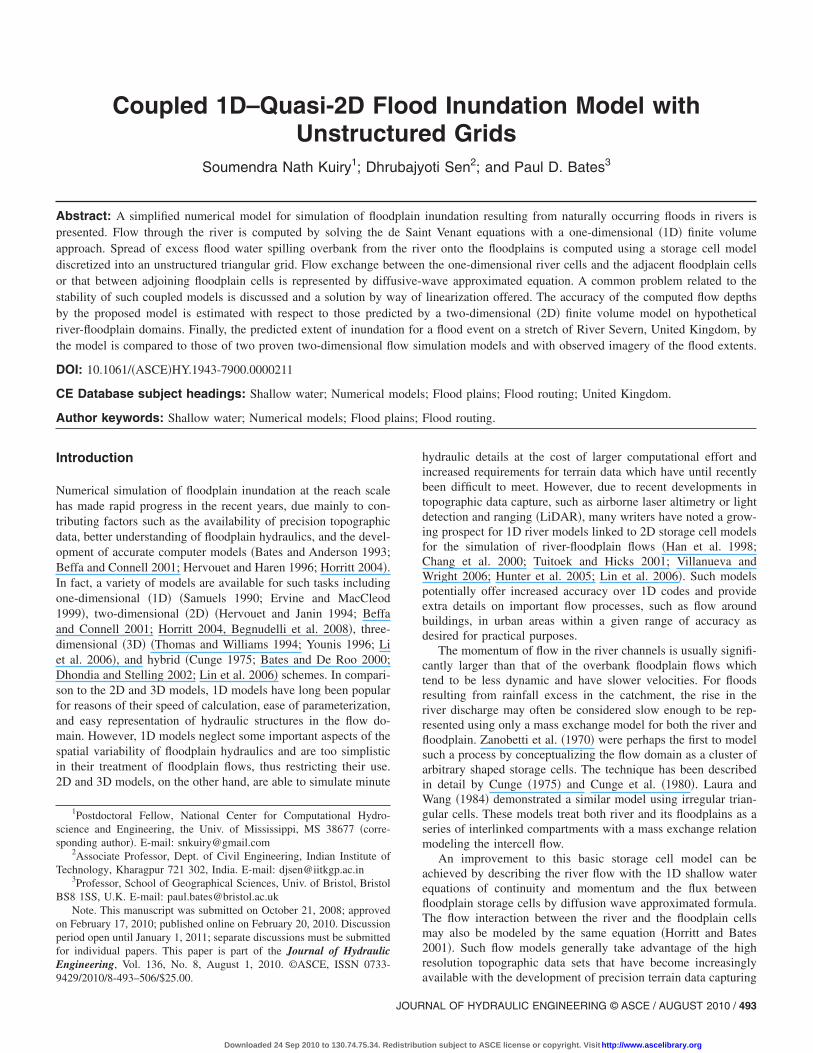
where Ai and Hi=plan area and water levels of cell i. Fig. 1�a�shows an assumed flow description for a floodplain cell i with itsneighboring cells.

An equation for the flow rate between two cells is derivedfrom the diffusive-wave approximation of the depth-averagedshallow water momentum equation �Bradbrook et al. 2004�. Thusthe flow exchange between two cells i and j may be expressed bythe following equation:

Qi,j =1

nbhflow

5/3 Hj − Hi

�xc�� Hj − Hi

�xc 1/2� �6�

where n=Manning’s coefficient of friction; b=length of the com-mon edge between cells i and j with water levels Hi and Hj,respectively, above a datum; and �xc=distance between the cen-troids of the cells. Though other approximations may be used, theproposed model defines the depth of flow between the two cellshflow �Fig. 1�b��, as the difference between the higher of the watersurfaces and the bed elevations of the two cells �Horritt and Bates2001�. Thus, if the bed elevations of the two cells are zbi

and zbj,

respectively, then hflow may be expressed as

hflow = max�Hi,Hj� − max�zbi,zbj

� �7�

It may be observed that in Eq. �6� the mean water surface gradientbetween the neighboring cells i and j is evaluated by joining thewater surfaces at the centroid of each cell.

Coupling of the 1D River and the Floodplain StorageCell Models

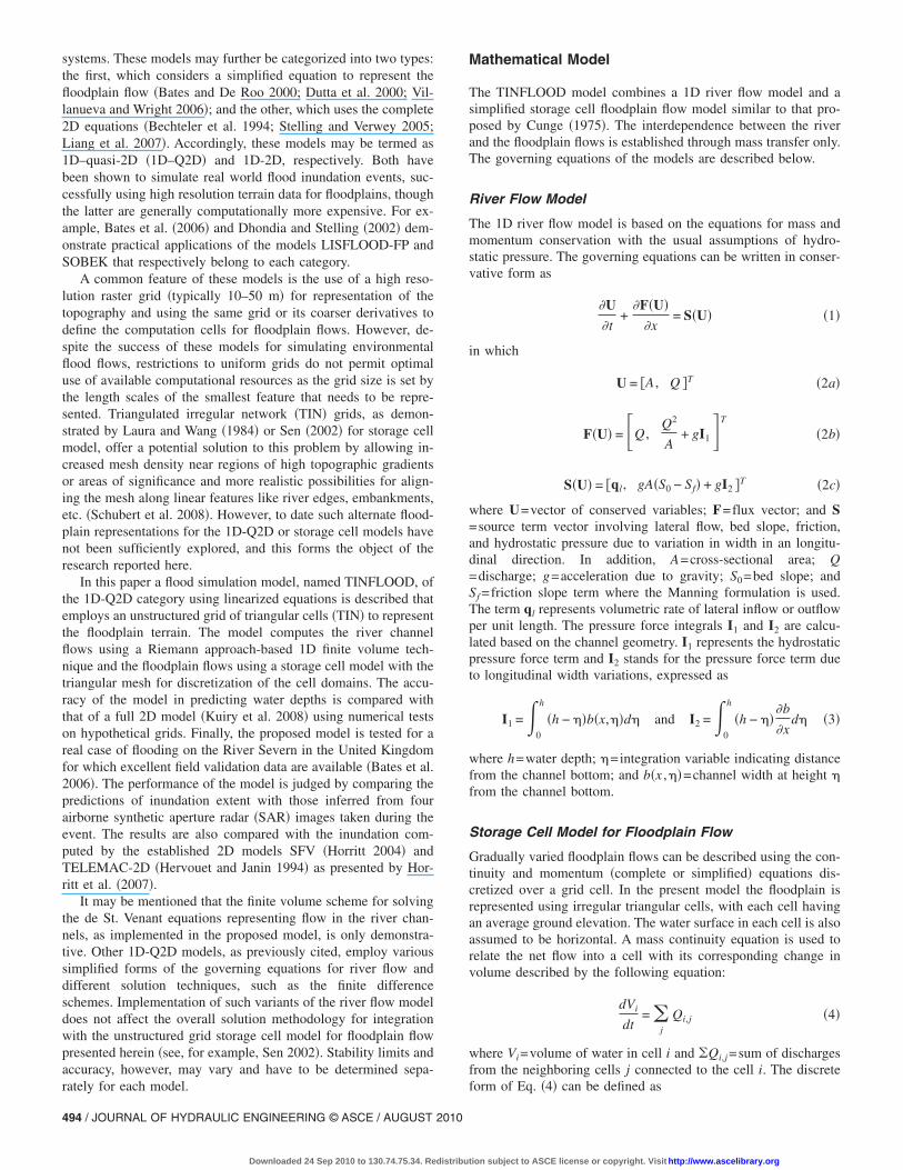
As a flood hydrograph passes through a river reach, the waterdepth for some of the river cells rise above their respective bank-full depths and the excess water overflows onto the floodplaincells adjacent to the river. Fig. 2�a� shows such a typical reachdiscretized into 1D cells and adjacent floodplain discretized intotriangular cells. Some of the river cells �2 and 3 in the figure� areconsidered overflowing their banks at this instant and are hydrau-lically connected to respective floodplain cells on the banks �A,D, and E�, as shown in the conceptual representation of masstransfer in Fig. 2�b�. All other floodplain cells shown shaded areassumed to be exchanging flows with the river cells and between

hflow

(a) (b)

Fig. 1. Flow description for a floodplain cell i

themselves at a given instant.

JOUR

Downloaded 24 Sep 2010 to 130.74.75.34. Redistribu

The flow interaction between a floodplain and a river cell isapproximated considering only mass transfer. An equation similarto Eq. �6� is used to model the flow to or from a river-adjacentflood plain cell. The same flows, but with opposite algebraicsigns, are also applied to the respective source terms �ql� of Eq.�1� for the corresponding river cells.

Flow Initiation and Termination

Initially all the floodplain cells are assumed to be dry and discon-nected from the river. As a flood wave passes through the riverand some stretches of its banks start overflowing, flow exchangeis initiated between the river cells and the corresponding flood-plain cells. The interior floodplain cells progressively become wetwith rising river water levels which is assumed to be primarilyresponsible for flood ingress. During recession, the river levelstarts falling and the floodplain cells except those in depressionsstart drying up. In order to initiate or terminate flow into or out ofa cell a threshold water level, the no-flow tolerance level �hnftol�,is specified and defined as

hnftol = max�zbi,zbj� + htol �8�

in which zbi and zbj =average bed elevations of cell i and itsneighboring cell j and htol is a tolerance depth, arbitrarily set at0.01 m. Thus, hnftol may vary within a cell for each of the threeedges depending upon the bed levels of the adjacent cells. De-pending upon the criteria mentioned above, several flow situa-tions are possible, as depicted in Fig. 3. The dotted line representsthe level hnftol. If the water levels of both the cells across an edgeare below hnftol, it is assumed that the cells are not hydraulicallyconnected �Figs. 3�a–c��; otherwise the flow is assumed to takeplace in the direction from the cell with higher water level to theone with lower water level across the edge �Figs. 3�d–i��. In thefigures, cell i is assumed to have a lower average bed level thanits neighboring cell j.

Numerical Solution of the Governing Equations

A cell-centered finite volume scheme based upon the Godunovapproach and the approximate Riemann solver of Roe �1981� isused to numerically solve the 1D river flow equations, consider-ing the source term contributions due to the lateral flows into the

(a)

(b)

Fig. 2. �a� Sample river reach showing some banks overflowing; �b�a river cell connected to an overflowing floodplain cell

river cells from the hydraulically connected floodplain cells or

NAL OF HYDRAULIC ENGINEERING © ASCE / AUGUST 2010 / 495

tion subject to ASCE license or copyright. Visit http://www.ascelibrary.org

vice versa. Under the wave splitting approach adopted with aRiemann solver the general form of the numerical scheme can bewritten as

�x

�t�Un+1 − Un� = − ���F̃i+1/2

n+1 − F̃i−1/2n+1 � − ��xSi

n+1

+ �1 − ���F̃i+1/2n − F̃i−1/2

n � − �1 − ���xSin� �9�

where the time weighting factor � may vary between 0 and 1;

F̃i�1/2 represent Roe averaged fluxes at cell interfaces with thecell averaged values defined at the cell centre i; �t=time step;and Un+1 and Un=vectors of conserved variables at new and oldtime steps, respectively. The numerical flux vector in Eq. �9� maybe written as

F̃i�1/2 =1

2�Fi + Fi�1 + R̃i�1/2�i�1/2� �10�

and can be derived for different vector functions �i�1/2. The de-tails of the Roe’s Riemann solver and its application to 1D shal-low water equations can be found in Hubbard �1999� and Delis etal. �2000�. The second-order accuracy in space is obtained usingthe surface gradient method proposed by Zhou et al. �2001� andthe bed slope source term is treated as suggested by Sanders et al.�2003�. A cellwise treatment is adopted for the friction term. Thusthe river flow model is shock capturing, second-order accurate inspace and suitable for nonrectangular and nonprismatic channels.

In the storage cell model the change in water level for a flood-plain cell is evaluated by solving Eq. �5�, written in an equivalentdiscrete form as

Ai

�t�Hi

n+1 − Hin� = ��

j

Qi,jn+1 + �1 − ���

j

Qi,jn �11�

where Hin and Hi

n+1=water levels of cell i at present and next timelevels, respectively. The solution methodology of the above equa-tions, Eqs. �9� and �11� as a coupled system, is presented in the

No Flow No Flow No Flow

Fig. 3. Possible flow situations between two floodplain cells i and j

following section.

496 / JOURNAL OF HYDRAULIC ENGINEERING © ASCE / AUGUST 2010

Downloaded 24 Sep 2010 to 130.74.75.34. Redistribu

Solution Scheme

The discretized equations for the river �Eq. �9�� and those of thehydraulically interacting flood plain cells �Eq. �11�� have to besolved together by an appropriate time-marching scheme. Initialvalues of the depths and velocities of the cell-centered river cellsand the water levels of the flood plain cells also need to be as-signed for commencing the solution process. Although explicitschemes may be employed as done for similar storage cell mod-els, for example, Bates and De Roo �2000�, a Euler implicit timeintegration scheme was implemented in the present model consid-ering �=1, making the solution fully implicit with first-order ac-curacy in time. The motivation for using an implicit solverstemmed mainly from the solution scheme of the River Mekongstorage cell model described by Cunge et al. �1980�, which wassolved by the double-sweep algorithm. An algorithm for generat-ing the least sparse matrix structure at a given time step �or at aniteration level� is described in the Appendix for the hypotheticalflow situation of Fig. 2�a�. These equations may be solved, amongother methods, by the Newton-Raphson technique to estimate thevariables in the next time step iteratively. Although computermemory may not be a limitation with the present generation ma-chines, the implicit formulation permits a dynamic assembly ofthe coefficients of the interacting flood plain cells at any instantfollowed by corresponding elimination and back substitution asproposed by Sen �2002�, which helps to keep the size of theoverall matrix a minimum. Additionally, for inundation from net-worked channels, as in the flood plains of river estuaries, thematrix of the flood plain cell coefficients may be domain decom-posed and conveniently integrated with those of the discretizedequations for looped or branched channels for solution by theimplicit algorithm of Sen and Garg �2002�.

Application of the solution scheme as proposed above, how-ever, produces occasional oscillations of the solved variables.Most often, these oscillations become noticeable only after thesimulation has progressed for some time. The instabilities appearto originate from the river and river-adjacent flood plain cells,spreading and amplifying to the entire domain within a short time.Using extremely small time step or large cell sizes may helpcircumvent the problem but could lead to either the model resultsbeing computationally expensive or the physical representationsbeing insufficiently resolved. A similar phenomenon, but for anexplicit model, has been described extensively by Hunter et al.�2005�. A complete elimination of the oscillations requires eitherthe introduction of some form of flux limiter or the implementa-tion of an adaptive time step �as, for example, the adaptive timestepping scheme of Hunter et al. 2005�. However, it has beenshown that flux limited solutions may be physically unrealisticand adaptive time stepping may still incur large computation coston fine grids �ibid�.

Linearization for Improved Model Stability

A study of several numerical test cases for flood plain inundationsindicates that the discharge variable in Eq. �11� and the lateraldischarge in the source term of the continuity expression of Eq.�9� are primarily responsible for the oscillatory solutions. Oneway to avoid this problem is to estimate the variables at the nexttime level by a timewise Taylor series expansion. This effectivelylinearizes the equations at a given time level and estimates thoseof the next level by a single iteration. This contrasts with the

tion subject to ASCE license or copyright. Visit http://www.ascelibrary.org

which comprises essentially of successive linearization stepswithin a time interval for the best guess at the next time level.

A first level of linearization is, therefore, attempted by substi-tuting the following Taylor series expansion in time for the flowdischarge as shown below:

Qi,jn+1 = Qi,j

n +�Qi,j

n

�Hi�Hi +

�Qi,jn

�Hj�Hj �12�

where �Hi=Hin+1−Hi

n and �Hj =Hjn+1−Hj

n. Substitution of Eq.�12� into Eq. �11� yields the following �with �=1�:

Ai

�t�Hi

n+1 − Hin� = �

j

Qi,jn + �

j

�Qi,jn

�Hi�Hi + �

j

�Qi,jn

�Hj�Hj�

�13�

After integrating the river flow equations along the length of acell for a finite volume discretization, the source term of the con-tinuity equation in Eq. �9�, is substituted by Eq. �12� and thefloodplain flow equation, Eq. �11�, is substituted by Eq. �13�.

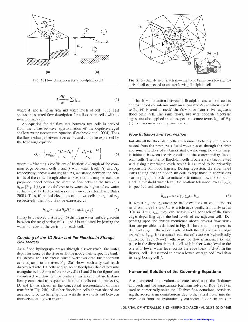
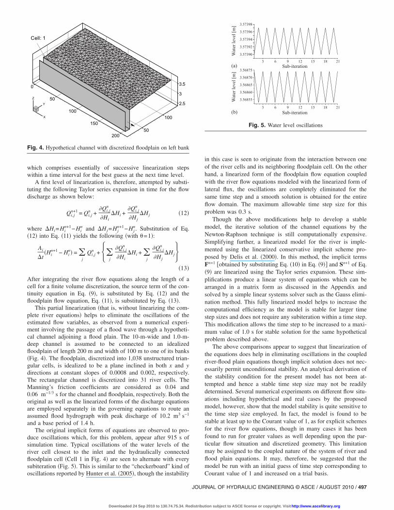
This partial linearization �that is, without linearizing the com-plete river equations� helps to eliminate the oscillations of theestimated flow variables, as observed from a numerical experi-ment involving the passage of a flood wave through a hypotheti-cal channel adjoining a flood plain. The 10-m-wide and 1.0-m-deep channel is assumed to be connected to an idealizedfloodplain of length 200 m and width of 100 m to one of its banks�Fig. 4�. The floodplain, discretized into 1,038 unstructured trian-gular cells, is idealized to be a plane inclined in both x and ydirections at constant slopes of 0.0008 and 0.002, respectively.The rectangular channel is discretized into 31 river cells. TheManning’s friction coefficients are considered as 0.04 and0.06 m−1/3 s for the channel and floodplain, respectively. Both theoriginal as well as the linearized forms of the discharge equationsare employed separately in the governing equations to route anassumed flood hydrograph with peak discharge of 10.2 m3 s−1

and a base period of 1.4 h.The original implicit forms of equations are observed to pro-

duce oscillations which, for this problem, appear after 915 s ofsimulation time. Typical oscillations of the water levels of theriver cell closest to the inlet and the hydraulically connectedfloodplain cell �Cell 1 in Fig. 4� are seen to alternate with everysubiteration �Fig. 5�. This is similar to the “checkerboard” kind of

Fig. 4. Hypothetical channel with discretized floodplain on left bank

oscillations reported by Hunter et al. �2005�, though the instability

JOUR

Downloaded 24 Sep 2010 to 130.74.75.34. Redistribu

in this case is seen to originate from the interaction between oneof the river cells and its neighboring floodplain cell. On the otherhand, a linearized form of the floodplain flow equation coupledwith the river flow equations modeled with the linearized form oflateral flux, the oscillations are completely eliminated for thesame time step and a smooth solution is obtained for the entireflow domain. The maximum allowable time step size for thisproblem was 0.3 s.

Though the above modifications help to develop a stablemodel, the iterative solution of the channel equations by theNewton-Raphson technique is still computationally expensive.Simplifying further, a linearized model for the river is imple-mented using the linearized conservative implicit scheme pro-posed by Delis et al. �2000�. In this method, the implicit termsFn+1 �obtained by substituting Eq. �10� in Eq. �9�� and Sn+1 of Eq.�9� are linearized using the Taylor series expansion. These sim-plifications produce a linear system of equations which can bearranged in a matrix form as discussed in the Appendix andsolved by a simple linear systems solver such as the Gauss elimi-nation method. This fully linearized model helps to increase thecomputational efficiency as the model is stable for larger timestep sizes and does not require any subiteration within a time step.This modification allows the time step to be increased to a maxi-mum value of 1.0 s for stable solution for the same hypotheticalproblem described above.

The above comparisons appear to suggest that linearization ofthe equations does help in eliminating oscillations in the coupledriver-flood plain equations though implicit solution does not nec-essarily permit unconditional stability. An analytical derivation ofthe stability condition for the present model has not been at-tempted and hence a stable time step size may not be readilydetermined. Several numerical experiments on different flow situ-ations including hypothetical and real cases by the proposedmodel, however, show that the model stability is quite sensitive tothe time step size employed. In fact, the model is found to bestable at least up to the Courant value of 1, as for explicit schemesfor the river flow equations, though in many cases it has beenfound to run for greater values as well depending upon the par-ticular flow situation and discretized geometry. This limitationmay be assigned to the coupled nature of the system of river andflood plain equations. It may, therefore, be suggested that themodel be run with an initial guess of time step corresponding to

3 6 9 12 15 18 21

3.57390

3.57392

3.57394

3.57396

3.57398

3 6 9 12 15 18 21

3.56855

3.56860

3.56865

3.56870

3.56875

Sub-iteration

Sub-iteration

Wat

erle

vel

[m]

Wat

erle

vel

[m]

(a)

(b)

Fig. 5. Water level oscillations

Courant value of 1 and increased on a trial basis.

NAL OF HYDRAULIC ENGINEERING © ASCE / AUGUST 2010 / 497

tion subject to ASCE license or copyright. Visit http://www.ascelibrary.org

Boundary Conditions

The proposed model TINFLOOD is developed to simulate thedynamic routing of a flood wave through a river reach and inun-dation of its adjacent floodplains due to overbank spillage. Thepossible boundary conditions that may be implemented in theriver and the floodplain models are discussed separately in thissection.

River Flow Model

For the finite volume solution of the river flow equations, theknown boundary variables are imposed at the inflow and outflowends of the river reach depending upon the given flow conditions.Solutions for the other dependent variables are found using themethod of characteristics, the details of which can be found inGarcía-Navarro and Savirón �1992� or Crossley �1999�. The otherboundary conditions included in the model are discussed below.

River Discharge at UpstreamAt the upstream boundary either a constant discharge or a time-varying discharge hydrograph can be imposed.

Water Level Specification at DownstreamEither a stage-discharge relation or the water level variation withtime may be specified at the downstream boundary. A normaldepth outflow condition can also be imposed for natural nontidalrivers.

Storage Cell Model

The storage cell model for the floodplain flow includes the fol-lowing boundary conditions.

Flow Boundary ConditionFor cells having edges coinciding with the inflow boundaries, thecorresponding discharges per unit width may be specified at theedges. The outflow through a cell edge for a given water depth orslope is approximated by a weir or a uniform flow formula, re-spectively.

No-Flow Boundary ConditionIf an edge of a floodplain cell coincides with an impermeableboundary, such as an embankment or a levee, a no-flow boundarycondition is implemented by assigning the total flow across that

0

500

1000

2000 4000

0

500

1000

0

500

1000

Fig. 6. Hypothetical channel and floodplains: �a� straight channel

edge as zero.

498 / JOURNAL OF HYDRAULIC ENGINEERING © ASCE / AUGUST 2010

Downloaded 24 Sep 2010 to 130.74.75.34. Redistribu

Model Accuracy

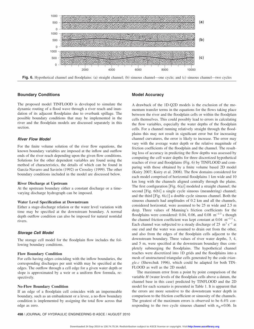
A drawback of the 1D-Q2D models is the exclusion of the mo-mentum transfer terms in the equations for the flows taking placebetween the river and the floodplain cells or within the floodplaincells themselves. This could possibly lead to errors in calculatingthe flow variables, especially the water depths of the floodplaincells. For a channel running relatively straight through the flood-plains this may not result in significant error but for increasingchannel curvatures, the error is likely to increase. The error mayvary with the average water depth or the relative magnitude offriction coefficients of the floodplain and the channel. The result-ing loss of accuracy in predicting the flow depths was assessed bycomputing the cell water depths for three discretized hypotheticalreaches of river and floodplains �Fig. 6� by TINFLOOD and com-paring with those obtained by a finite volume based 2D model�Kuiry 2007; Kuiry et al. 2008�. The flow domains considered foreach model comprised of horizontal floodplains 1 km wide and 10km long with the channels aligned centrally through the plains.The first configuration �Fig. 6�a�� modeled a straight channel; thesecond �Fig. 6�b�� a single cycle sinuous �meandering� channel;and the third �Fig. 6�c�� a double cycle sinuous channel. Both thesinuous channels had amplitudes of 0.2 km and all the channels,considered horizontal, were assumed to be 25 m wide and 2.5 mdeep. Three values of Manning’s friction coefficients for thefloodplains were considered: 0.04, 0.06, and 0.08 m−1/3 s thoughthe channel friction coefficient was kept constant at 0.04 m−1/3 s.Each channel was subjected to a steady discharge of 25 m3 s−1 atone end and the water was assumed to drain out from the other,and also from the edges of the floodplain cells adjacent to thedownstream boundary. Three values of river water depths, 3, 4,and 5 m, were specified at the downstream boundary thus com-pletely submerging the floodplains. The hypothetical channelreaches were discretized into 1D grids and the floodplains into amesh of unstructured triangular cells generated by the code trian-gle.c �Shewchuk 1996�, which could be adapted for both TIN-FLOOD as well as the 2D model.

The maximum error from a point by point comparison of thevariable H �water levels of the floodplain cells above a datum, thechannel base in this case� predicted by TINFLOOD and the 2Dmodel for each scenario is presented in Table 1. It is apparent thatthe errors are more sensitive to the downstream water depth incomparison to the friction coefficient or sinuosity of the channels.The greatest of the maximum errors is observed to be 6.4% cor-

6000 8000 10000

( )a

( )b

( )c

inuous channel—one cycle; and �c� sinuous channel—two cycles

responding to the two cycle sinuous channel with nfp=0.06. In

tion subject to ASCE license or copyright. Visit http://www.ascelibrary.org

this case the root mean square error normalized with the averageH value is estimated to be 0.0354.

The above investigations, carried out with steady-state flowconditions, provide a fair estimate of the accuracy �or the loss ofit� by the 1D-Q2D model on ignoring the momentum exchangebetween the river and the floodplain cells. However, in addition, asecond set of tests were conducted to assess the predictive abilityof the model in computing floodplain depths for a flood wave.Only the straight channel configuration �Fig. 6�a�� was consideredwith Manning’s friction coefficients assumed as 0.02 and0.06 m−1/3 s, respectively, for the channel and the floodplains. Anarbitrary base flow �Qb� of 100 m3 s−1 was assumed for the chan-nel that completely submerged the floodplains under a constantdownstream water depth of 3 m measured above the channel bot-tom. Idealized triangular-shaped flood hydrographs, with peakdischarges �Qp� varying from two, three, and four times the baseflow were applied on the upstream. The total duration of the floodwave �base time tb� in each case was maintained as 4 h but thetime to peak �tp� was varied between 1, 2, and 3 h. Thus theexperiment consisted of nine different hydrographs, for each ofwhich the flow depths were tracked at three positions, A, B, andC, on the floodplain, arbitrarily chosen along half the floodplainwidth and at one-fourth, half, and three-fourths its length. Thecoordinates of the points therefore, in meters, were �2,500, 250�,�5,000, 250� and �7,500, 250� respectively, in the grid of Fig. 6�a�.

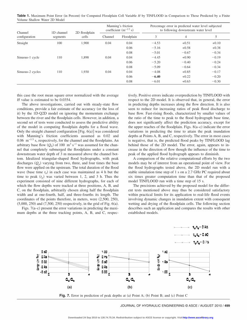
Figs. 7�a–c� present the error variations in predicting the maxi-mum depths at the three tracking points, A, B, and C, respec-

Table 1. Maximum Point Error �in Percent� for Computed Floodplain CVolume Shallow Water 2D Model

Channelconfiguration

1D channelsegments

2D floodplaincells

Manningcoefficien

Channel

Straight 100 1,900 0.04

Sinuous-1 cycle 110 1,898 0.04

Sinuous-2 cycles 110 1,930 0.04

(a)

Fig. 7. Error in prediction of peak depth

JOUR

Downloaded 24 Sep 2010 to 130.74.75.34. Redistribu

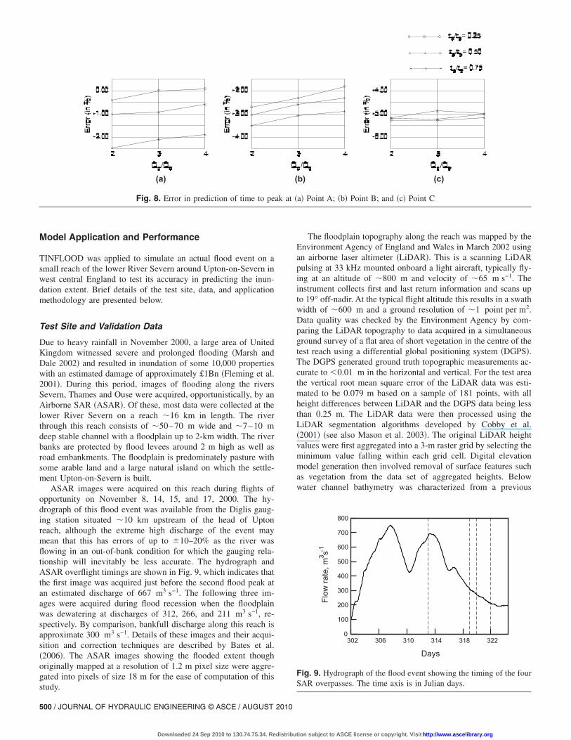
tively. Positive errors indicate overprediction by TINFLOOD withrespect to the 2D model. It is observed that, in general, the errorin predicting depths increases along the flow direction. It is alsoseen to reduce for increasing ratios of peak flood discharge tobase flow. Fast-rising floods, characterized by smaller values ofthe ratio of the time to peak to the flood hydrograph base time,does not significantly affect the prediction accuracy, except forthe upper reaches of the floodplain. Figs. 8�a–c� indicate the errorvariations in predicting the time to attain the peak inundationdepths at Points A, B, and C, respectively. The error in most casesis negative, that is, the predicted flood peaks by TINFLOOD lagbehind those of the 2D model. The error, again, appears to in-crease in the direction of flow though the influence of the time topeak of the applied flood hydrograph appears to diminish.

A comparison of the relative computational efforts by the twomodels may be of interest from an operational point of view. Forthe flood hydrographs tested above, the 2D model run with astable simulation time step of 1 s on a 2.7 GHz PC required aboutsix times greater computation time than that of the proposedmodel TINFLOOD run with a time step of 15 s.

The precisions achieved by the proposed model for the differ-ent tests mentioned above may thus be considered satisfactorywithin practical limits for its application to real-life flood eventsinvolving dynamic changes in inundation extent with consequentwetting and drying of the floodplain cells. The following sectiondescribes such an application and compares the results with otherestablished models.

riable H by TINFLOOD in Comparison to Those Predicted by a Finite

ion3 s�

Percentage error in predicted water level subjectedto following downstream water level

dplain 3 4 5

.04 �4.53 +0.51 +0.10

.06 �5.16 +0.58 +0.38

.08 �5.01 �0.67 �0.34

.04 �4.45 +0.90 �0.19

.06 �5.20 �0.40 �0.24

.08 �5.09 �0.64 �0.34

.04 �4.08 +0.85 �0.17

.06 �6.40 +0.22 �0.20

.08 �6.01 +0.63 �0.30

b) (c)

� Point A; �b� Point B; and �c� Point C

ell Va

’s frictt �m−1/

Floo

0

0

0

0

0

0

0

0

0

(

s at �a

NAL OF HYDRAULIC ENGINEERING © ASCE / AUGUST 2010 / 499

tion subject to ASCE license or copyright. Visit http://www.ascelibrary.org

Model Application and Performance

TINFLOOD was applied to simulate an actual flood event on asmall reach of the lower River Severn around Upton-on-Severn inwest central England to test its accuracy in predicting the inun-dation extent. Brief details of the test site, data, and applicationmethodology are presented below.

Test Site and Validation Data

Due to heavy rainfall in November 2000, a large area of UnitedKingdom witnessed severe and prolonged flooding �Marsh andDale 2002� and resulted in inundation of some 10,000 propertieswith an estimated damage of approximately £1Bn �Fleming et al.2001�. During this period, images of flooding along the riversSevern, Thames and Ouse were acquired, opportunistically, by anAirborne SAR �ASAR�. Of these, most data were collected at thelower River Severn on a reach �16 km in length. The riverthrough this reach consists of �50–70 m wide and �7–10 mdeep stable channel with a floodplain up to 2-km width. The riverbanks are protected by flood levees around 2 m high as well asroad embankments. The floodplain is predominately pasture withsome arable land and a large natural island on which the settle-ment Upton-on-Severn is built.

ASAR images were acquired on this reach during flights ofopportunity on November 8, 14, 15, and 17, 2000. The hy-drograph of this flood event was available from the Diglis gaug-ing station situated �10 km upstream of the head of Uptonreach, although the extreme high discharge of the event maymean that this has errors of up to �10–20% as the river wasflowing in an out-of-bank condition for which the gauging rela-tionship will inevitably be less accurate. The hydrograph andASAR overflight timings are shown in Fig. 9, which indicates thatthe first image was acquired just before the second flood peak atan estimated discharge of 667 m3 s−1. The following three im-ages were acquired during flood recession when the floodplainwas dewatering at discharges of 312, 266, and 211 m3 s−1, re-spectively. By comparison, bankfull discharge along this reach isapproximate 300 m3 s−1. Details of these images and their acqui-sition and correction techniques are described by Bates et al.�2006�. The ASAR images showing the flooded extent thoughoriginally mapped at a resolution of 1.2 m pixel size were aggre-gated into pixels of size 18 m for the ease of computation of this

(a)

Fig. 8. Error in prediction of time to pe

study.

500 / JOURNAL OF HYDRAULIC ENGINEERING © ASCE / AUGUST 2010

Downloaded 24 Sep 2010 to 130.74.75.34. Redistribu

The floodplain topography along the reach was mapped by theEnvironment Agency of England and Wales in March 2002 usingan airborne laser altimeter �LiDAR�. This is a scanning LiDARpulsing at 33 kHz mounted onboard a light aircraft, typically fly-ing at an altitude of �800 m and velocity of �65 m s−1. Theinstrument collects first and last return information and scans upto 19° off-nadir. At the typical flight altitude this results in a swathwidth of �600 m and a ground resolution of �1 point per m2.Data quality was checked by the Environment Agency by com-paring the LiDAR topography to data acquired in a simultaneousground survey of a flat area of short vegetation in the centre of thetest reach using a differential global positioning system �DGPS�.The DGPS generated ground truth topographic measurements ac-curate to �0.01 m in the horizontal and vertical. For the test areathe vertical root mean square error of the LiDAR data was esti-mated to be 0.079 m based on a sample of 181 points, with allheight differences between LiDAR and the DGPS data being lessthan 0.25 m. The LiDAR data were then processed using theLiDAR segmentation algorithms developed by Cobby et al.�2001� �see also Mason et al. 2003�. The original LiDAR heightvalues were first aggregated into a 3-m raster grid by selecting theminimum value falling within each grid cell. Digital elevationmodel generation then involved removal of surface features suchas vegetation from the data set of aggregated heights. Belowwater channel bathymetry was characterized from a previous

b) (c)

a� Point A; �b� Point B; and �c� Point C

0

100

200

300

400

500

600

700

800

302 306 310 314 318 322

Flo

wra

te,m

3s-1

Days

Fig. 9. Hydrograph of the flood event showing the timing of the fourSAR overpasses. The time axis is in Julian days.

(

ak at �

tion subject to ASCE license or copyright. Visit http://www.ascelibrary.org

ground survey consisting of �20 cross sections conducted by theEnvironment Agency and supplemented by a boat survey at asmall number of key locations conducted in autumn 2003.

Model Application and Results

The computational grid of the region for running the TINFLOODmodel was adapted from one of the two grids used by Horritt etal. �2007�, who had simulated the same flood using the 2D mod-els, SFV and TELEMAC-2D. These codes, based upon finite vol-ume and finite-element methodologies, respectively, employunstructured triangular grids for computing river and floodplainflows. The coarser grid used by the models comprised of 1,811nodes/3,486 elements while the finer had 6,172 nodes/12,097 el-ements. However, since the detailed studies did not show signifi-cant difference in predictions by either model on using the twogrids, only the coarser grid was adapted for the TINFLOOD stud-ies. In this case, the triangular cells in the river reach were re-placed with 1D river cells of rectangular cross sections withvarying bottom width as required by the model, which resulted in1,483 nodes/2,523 cells for the floodplains.

Table 2. Parameter Description Used to Calculate Measure of Fit

Model wet Model dry

SAR wet A C

SAR dry B —

Note: Class A represents the area predicted correctly and B and C areerrors.

(a )

(c )

Fig. 10. F scores: �a� Comparison 1; �a� Com

JOUR

Downloaded 24 Sep 2010 to 130.74.75.34. Redistribu

In order to simplify the calibration process, a single value ofManning’s friction coefficient �nch� was used for the channel seg-ments and another �nfp� for the floodplain cells. However, in orderto assess the best combination of nch and nfp, these were variedbetween 0.01 to 0.05 and 0.05 to 0.10, respectively. For eachcombination, dynamic TINFLOOD simulations were carried outwith the given inflow hydrograph �Fig. 9� as a time-varying fluxat the head of the channel. The time step for the simulations wasnormally kept at 200 s, except for the combinations with very lowvalues of nch and nfp.

Model prediction of inundation extents at the time of eachASAR overpass were compared with the corresponding observedimages of flood extent. This was done by resampling the simu-lated water depths over the domain into a binary wet/dry map bydifferencing the ground elevation from the water level at eachpoint. This map could be readily compared with the ASAR im-ages and the following goodness of fit function evaluated:

F =A

A + B + C�14�

where A, B, and C represent areas predicted wet or dry by themodel and observed from the ASAR data �Table 2�.

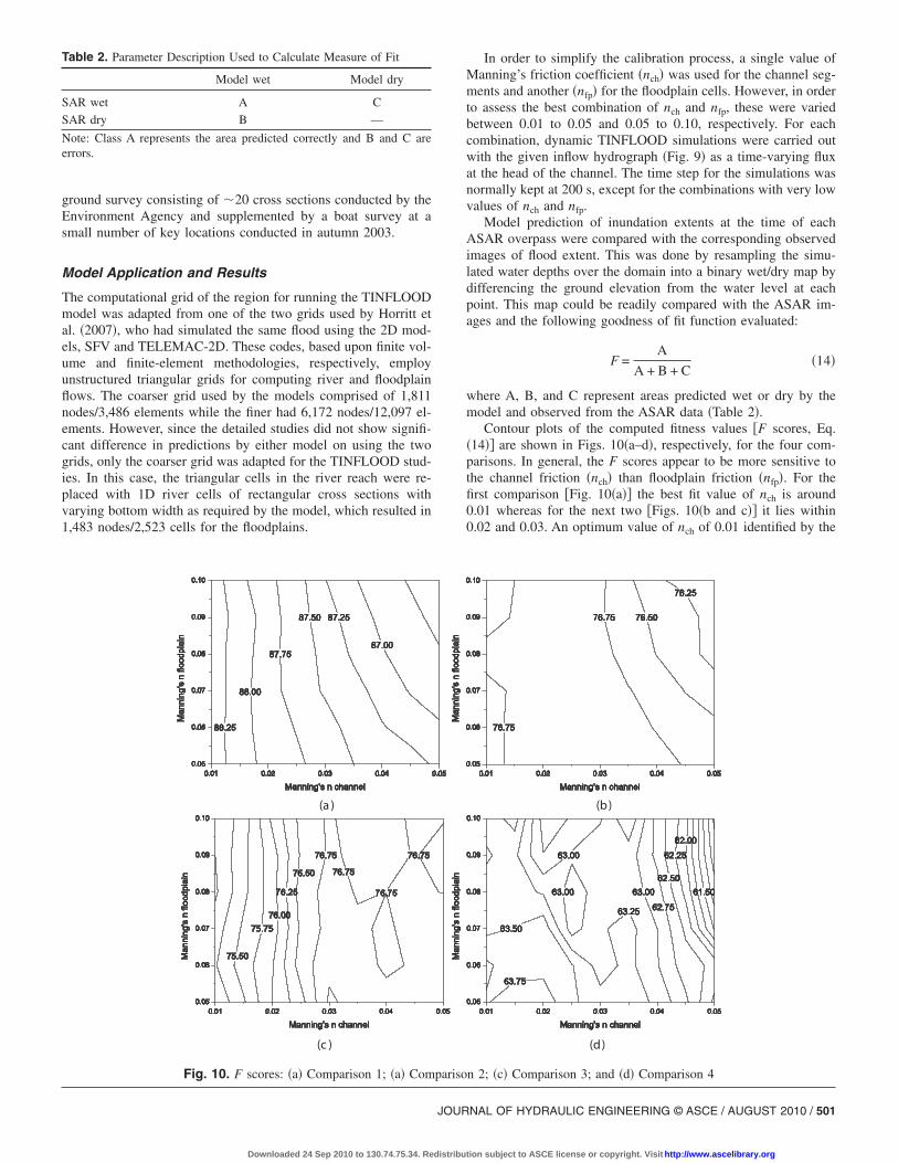
Contour plots of the computed fitness values �F scores, Eq.�14�� are shown in Figs. 10�a–d�, respectively, for the four com-parisons. In general, the F scores appear to be more sensitive tothe channel friction �nch� than floodplain friction �nfp�. For thefirst comparison �Fig. 10�a�� the best fit value of nch is around0.01 whereas for the next two �Figs. 10�b and c�� it lies within0.02 and 0.03. An optimum value of nch of 0.01 identified by the

(b)

(d)

n 2; �c� Comparison 3; and �d� Comparison 4

NAL OF HYDRAULIC ENGINEERING © ASCE / AUGUST 2010 / 501

tion subject to ASCE license or copyright. Visit http://www.ascelibrary.org

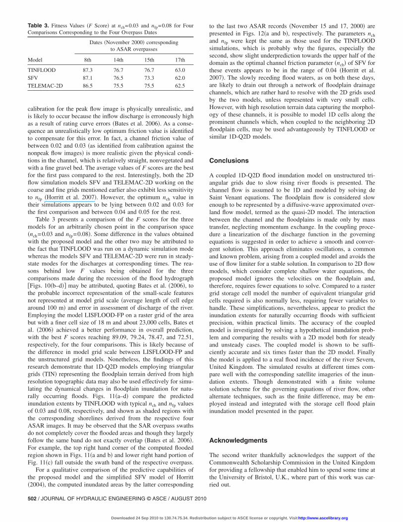
calibration for the peak flow image is physically unrealistic, andis likely to occur because the inflow discharge is erroneously highas a result of rating curve errors �Bates et al. 2006�. As a conse-quence an unrealistically low optimum friction value is identifiedto compensate for this error. In fact, a channel friction value ofbetween 0.02 and 0.03 �as identified from calibration against thenonpeak flow images� is more realistic given the physical condi-tions in the channel, which is relatively straight, nonvegetated andwith a fine gravel bed. The average values of F scores are the bestfor the first pass compared to the rest. Interestingly, both the 2Dflow simulation models SFV and TELEMAC-2D working on thecoarse and fine grids mentioned earlier also exhibit less sensitivityto nfp �Horritt et al. 2007�. However, the optimum nch value intheir simulations appears to be lying between 0.02 and 0.03 forthe first comparison and between 0.04 and 0.05 for the rest.

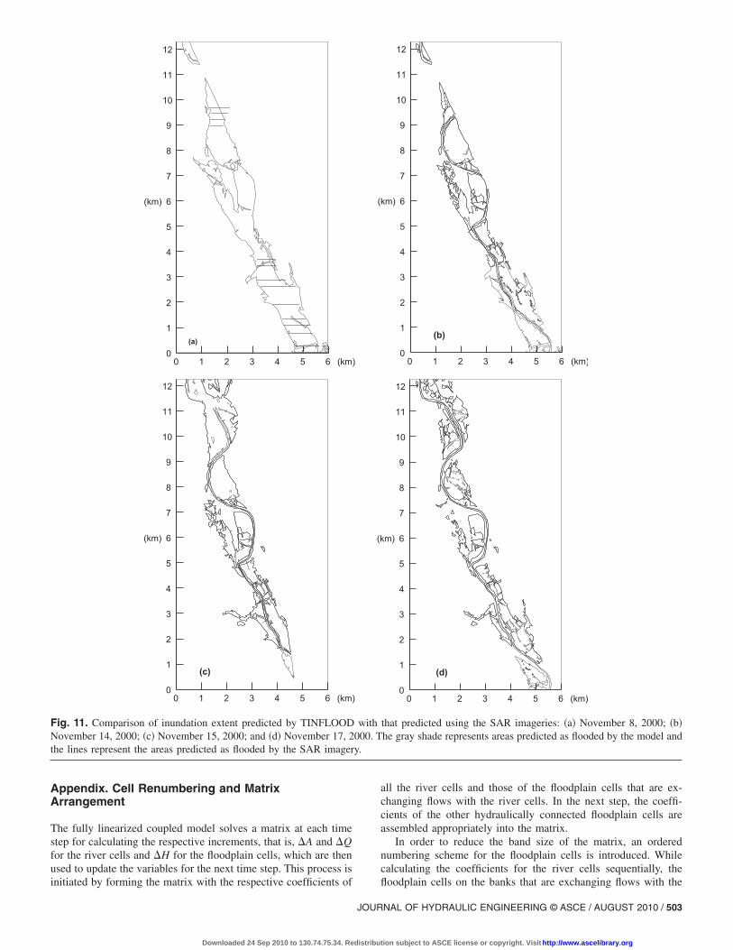
Table 3 presents a comparison of the F scores for the threemodels for an arbitrarily chosen point in the comparison space�nch=0.03 and nfp=0.08�. Some difference in the values obtainedwith the proposed model and the other two may be attributed tothe fact that TINFLOOD was run on a dynamic simulation modewhereas the models SFV and TELEMAC-2D were run in steady-state modes for the discharges at corresponding times. The rea-sons behind low F values being obtained for the threecomparisons made during the recession of the flood hydrograph�Figs. 10�b–d�� may be attributed, quoting Bates et al. �2006�, tothe probable incorrect representation of the small-scale featuresnot represented at model grid scale �average length of cell edgearound 100 m� and error in assessment of discharge of the river.Employing the model LISFLOOD-FP on a raster grid of the areabut with a finer cell size of 18 m and about 23,000 cells, Bates etal. �2006� achieved a better performance in overall prediction,with the best F scores reaching 89.09, 79.24, 78.47, and 72.51,respectively, for the four comparisons. This is likely because ofthe difference in model grid scale between LISFLOOD-FP andthe unstructured grid models. Nonetheless, the findings of thisresearch demonstrate that 1D-Q2D models employing triangulargrids �TIN� representing the floodplain terrain derived from highresolution topographic data may also be used effectively for simu-lating the dynamical changes in floodplain inundation for natu-rally occurring floods. Figs. 11�a–d� compare the predictedinundation extents by TINFLOOD with typical nch and nfp valuesof 0.03 and 0.08, respectively, and shown as shaded regions withthe corresponding shorelines derived from the respective fourASAR images. It may be observed that the SAR overpass swathsdo not completely cover the flooded areas and though they largelyfollow the same band do not exactly overlap �Bates et al. 2006�.For example, the top right hand corner of the computed floodedregion shown in Figs. 11�a and b� and lower right hand portion ofFig. 11�c� fall outside the swath band of the respective overpass.

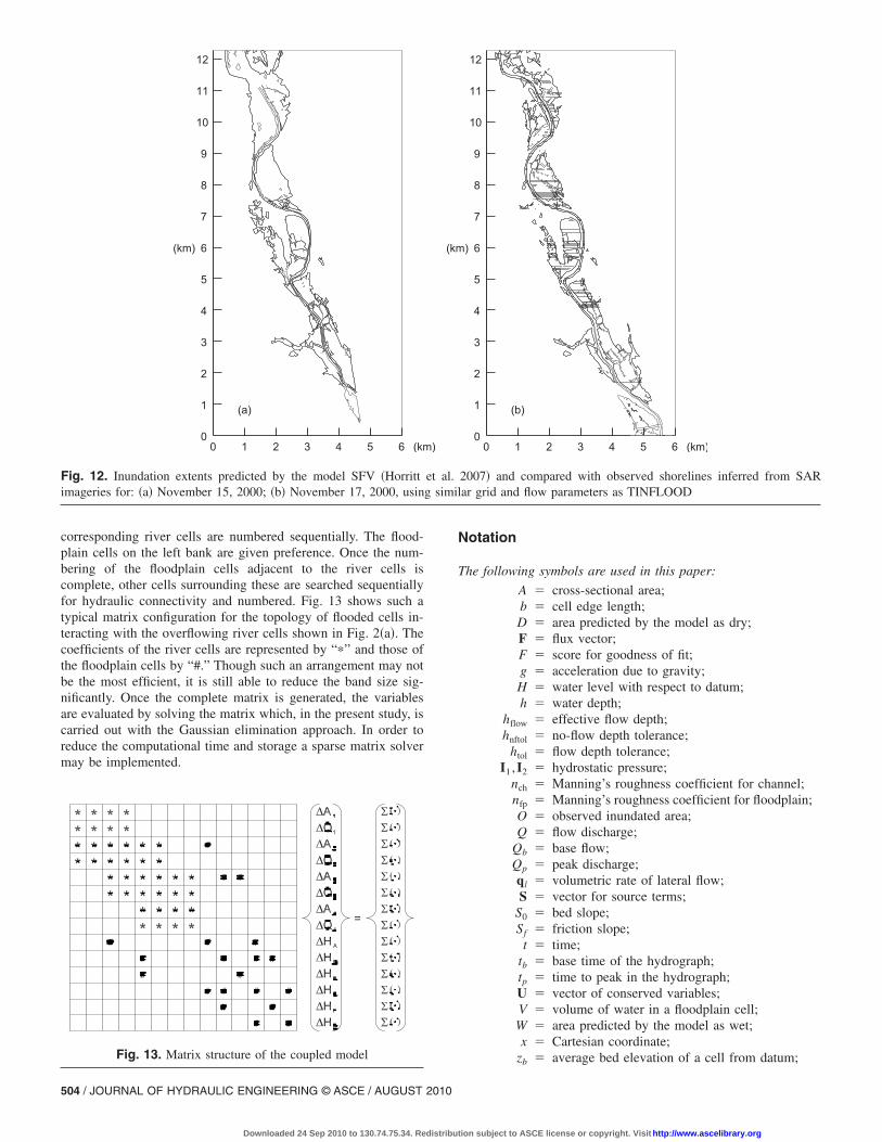
For a qualitative comparison of the predictive capabilities ofthe proposed model and the simplified SFV model of Horritt

Table 3. Fitness Values �F Score� at nch=0.03 and nfp=0.08 for FourComparisons Corresponding to the Four Overpass Dates

Model

Dates �November 2000� correspondingto ASAR overpasses

8th 14th 15th 17th

TINFLOOD 87.3 76.7 76.7 63.0

SFV 87.1 76.5 73.3 62.0

TELEMAC-2D 86.5 75.5 75.5 62.5

�2004�, the computed inundated areas by the latter corresponding

502 / JOURNAL OF HYDRAULIC ENGINEERING © ASCE / AUGUST 2010

Downloaded 24 Sep 2010 to 130.74.75.34. Redistribu

to the last two ASAR records �November 15 and 17, 2000� arepresented in Figs. 12�a and b�, respectively. The parameters nch

and nfp were kept the same as those used for the TINFLOODsimulations, which is probably why the figures, especially thesecond, show slight underprediction towards the upper half of thedomain as the optimal channel friction parameter �nch� of SFV forthese events appears to be in the range of 0.04 �Horritt et al.2007�. The slowly receding flood waters, as on both these days,are likely to drain out through a network of floodplain drainagechannels, which are rather hard to resolve with the 2D grids usedby the two models, unless represented with very small cells.However, with high resolution terrain data capturing the morphol-ogy of these channels, it is possible to model 1D cells along theprominent channels which, when coupled to the neighboring 2Dfloodplain cells, may be used advantageously by TINFLOOD orsimilar 1D-Q2D models.

Conclusions

A coupled 1D-Q2D flood inundation model on unstructured tri-angular grids due to slow rising river floods is presented. Thechannel flow is assumed to be 1D and modeled by solving deSaint Venant equations. The floodplain flow is considered slowenough to be represented by a diffusive-wave approximated over-land flow model, termed as the quasi-2D model. The interactionbetween the channel and the floodplains is made only by masstransfer, neglecting momentum exchange. In the coupling proce-dure a linearization of the discharge function in the governingequations is suggested in order to achieve a smooth and conver-gent solution. This approach eliminates oscillations, a commonand known problem, arising from a coupled model and avoids theuse of flow limiter for a stable solution. In comparison to 2D flowmodels, which consider complete shallow water equations, theproposed model ignores the velocities on the floodplain and,therefore, requires fewer equations to solve. Compared to a rastergrid storage cell model the number of equivalent triangular gridcells required is also normally less, requiring fewer variables tohandle. These simplifications, nevertheless, appear to predict theinundation extents for naturally occurring floods with sufficientprecision, within practical limits. The accuracy of the coupledmodel is investigated by solving a hypothetical inundation prob-lem and comparing the results with a 2D model both for steadyand unsteady cases. The coupled model is shown to be suffi-ciently accurate and six times faster than the 2D model. Finallythe model is applied to a real flood incidence of the river Severn,United Kingdom. The simulated results at different times com-pare well with the corresponding satellite imageries of the inun-dation extents. Though demonstrated with a finite volumesolution scheme for the governing equations of river flow, otheralternate techniques, such as the finite difference, may be em-ployed instead and integrated with the storage cell flood plaininundation model presented in the paper.

Acknowledgments

The second writer thankfully acknowledges the support of theCommonwealth Scholarship Commission in the United Kingdomfor providing a fellowship that enabled him to spend some time atthe University of Bristol, U.K., where part of this work was car-

tion subject to ASCE license or copyright. Visit http://www.ascelibrary.org

Appendix. Cell Renumbering and MatrixArrangement

The fully linearized coupled model solves a matrix at each timestep for calculating the respective increments, that is, �A and �Qfor the river cells and �H for the floodplain cells, which are thenused to update the variables for the next time step. This process is

0 1 2 3 4 5 6 (km)0

1

2

3

4

5

6(km)

7

8

9

10

11

12

(c)

0 1 2 3 4 5 6 (km)0

1

2

3

4

5

6(km)

7

8

9

10

11

12

(a)

Fig. 11. Comparison of inundation extent predicted by TINFLOODNovember 14, 2000; �c� November 15, 2000; and �d� November 17, 2the lines represent the areas predicted as flooded by the SAR imager

initiated by forming the matrix with the respective coefficients of

JOUR

Downloaded 24 Sep 2010 to 130.74.75.34. Redistribu

all the river cells and those of the floodplain cells that are ex-changing flows with the river cells. In the next step, the coeffi-cients of the other hydraulically connected floodplain cells areassembled appropriately into the matrix.

In order to reduce the band size of the matrix, an orderednumbering scheme for the floodplain cells is introduced. Whilecalculating the coefficients for the river cells sequentially, the

0 1 2 3 4 5 6 (km)0

1

2

3

4

5

6km)

7

8

9

10

11

12

(b)

0 1 2 3 4 5 6 (km)0

1

2

3

4

5

6m)

7

8

9

10

11

12

(d)

that predicted using the SAR imageries: �a� November 8, 2000; �b�he gray shade represents areas predicted as flooded by the model and

(

(k

with000. Ty.

floodplain cells on the banks that are exchanging flows with the

NAL OF HYDRAULIC ENGINEERING © ASCE / AUGUST 2010 / 503

tion subject to ASCE license or copyright. Visit http://www.ascelibrary.org

corresponding river cells are numbered sequentially. The flood-plain cells on the left bank are given preference. Once the num-bering of the floodplain cells adjacent to the river cells iscomplete, other cells surrounding these are searched sequentiallyfor hydraulic connectivity and numbered. Fig. 13 shows such atypical matrix configuration for the topology of flooded cells in-teracting with the overflowing river cells shown in Fig. 2�a�. Thecoefficients of the river cells are represented by “�” and those ofthe floodplain cells by “#.” Though such an arrangement may notbe the most efficient, it is still able to reduce the band size sig-nificantly. Once the complete matrix is generated, the variablesare evaluated by solving the matrix which, in the present study, iscarried out with the Gaussian elimination approach. In order toreduce the computational time and storage a sparse matrix solvermay be implemented.

(a)

0 1 2 3 4 5 6 (km0

1

2

3

4

5

6(km)

7

8

9

10

11

12

Fig. 12. Inundation extents predicted by the model SFV �Horrittimageries for: �a� November 15, 2000; �b� November 17, 2000, usin

Fig. 13. Matrix structure of the coupled model

504 / JOURNAL OF HYDRAULIC ENGINEERING © ASCE / AUGUST 2010

Downloaded 24 Sep 2010 to 130.74.75.34. Redistribu

Notation

The following symbols are used in this paper:

A � cross-sectional area;b � cell edge length;D � area predicted by the model as dry;F � flux vector;F � score for goodness of fit;g � acceleration due to gravity;H � water level with respect to datum;h � water depth;

hflow � effective flow depth;hnftol � no-flow depth tolerance;

htol � flow depth tolerance;I1 ,I2 � hydrostatic pressure;

nch � Manning’s roughness coefficient for channel;nfp � Manning’s roughness coefficient for floodplain;O � observed inundated area;Q � flow discharge;

Qb � base flow;Qp � peak discharge;ql � volumetric rate of lateral flow;S � vector for source terms;

S0 � bed slope;Sf � friction slope;

t � time;tb � base time of the hydrograph;tp � time to peak in the hydrograph;U � vector of conserved variables;V � volume of water in a floodplain cell;W � area predicted by the model as wet;x � Cartesian coordinate;

z � average bed elevation of a cell from datum;

(b)

0 1 2 3 4 5 6 (km)0

1

2

3

4

5

6)

7

8

9

10

11

12

2007� and compared with observed shorelines inferred from SARlar grid and flow parameters as TINFLOOD

)

(km

et al.g simi

b

tion subject to ASCE license or copyright. Visit http://www.ascelibrary.org

� � finite difference operator;�xc � distance between centroid of two neighboring

cells;� � integration variable indicating distance from

channel bed; and� � time weighting factor.

References

Bates, P. D., and Anderson, M. G. �1993�. “A two-dimensional finite-element model for river flow inundation.” Proc. R. Soc. London, Ser.A, 440, 481–491.

Bates, P. D., and De Roo, A. P. J. �2000�. “A simple raster based modelfor flood inundation simulation.” J. Hydrol., 236, 54–77.

Bates, P. D., Wilson, M. D., Horritt, M. S., Mason, D. C., Holden, N., andCurrie, A. �2006�. “Reach scale floodplain inundation dynamics ob-served using airborne synthetic aperture radar imagery: Data analysisand modelling.” J. Hydrol., 328, 306–318.

Bechteler, W., Hartman, S., and Otto, A. �1994�. “Coupling of 2D and 1Dmodels and integration into geographic information systems GIS.”River flood hydraulics, W. White and J. Watts, eds., Wiley, New York,155–165.

Beffa, C., and Connell, R. J. �2001�. “Two-dimensional flood plain flow.I: Model description.” J. Hydrol. Eng., 6�5�, 397–405.

Begnudelli, L., Sanders, B. F., and Bradford, S. F. �2008�. “AdaptiveGodunov-based model for flood simulation.” J. Hydraul. Eng.,134�6�, 714–725.

Bradbrook, K. F., Lane, S. N., Waller, S. G., and Bates, P. D. �2004�.“Two dimensional diffusion wave modelling of flood inundation usinga simplified channel representation.” Int. J. Riv. Basin. Manag, 2�3�,211–223.

Chang, T.-J., Hsu, M.-H., and Huang, C.-J. �2000�. “A GIS distributedwatershed model for simulating flooding and inundation.” J. Am.Water Resour. Assoc., 36, 975–988.

Cobby, D. M., Mason, D. C., and Davenport, I. J. �2001�. “Image pro-cessing of airborne scanning laser altimetry for improved river floodmodelling.” ISPRS J. Photogramm. Remote Sens., 56, 121–138.

Crossley, A. J. �1999�. “Accurate and efficient numerical solutions for theSaint Venant equations of open channel flow.” Ph.D. thesis, Univ. ofNottingham, Nottingham, U.K.

Cunge, J. A. �1975�. “Section 17: Two-dimensional modelling of floodplains.” Unsteady flow in open channels, K. Mahmood and V.Yevjevich, eds., Vol. II, Water Resources Publication, Colo., 17.705–17.762.

Cunge, J. A., Holly, F. M., and Verwey, A. �1980�. Practical aspects ofcomputational river hydraulics, Pitman Publishing Limited, London.

Delis, A. I., Skeels, C. P., and Ryrie, S. C. �2000�. “Implicit-high reso-lution methods for modelling one-dimensional open channel flow.” J.Hydraul. Res., 38, 369–382.

Dhondia, J. F., and Stelling, G. S. �2002�. “Application of onedimensional-two-dimensional integrated hydraulic model for floodsimulation and damage assessment.” Proc., 5th Int. Conf. on Hydroin-formatics 2002, R. Falconer, B. Bin, E. Harris, and C. Wilson, eds.,IWA Publishing, London, U.K., 265–276.

Dutta, D., Herath, S., and Musiake, K. �2000�. “Flood inundation simu-lation in a river basin using a physically distributed hydrologicalmodel.” Hydrolog. Process., 14, 497–519.

Ervine, D. A., and MacCleod, A. B. �1999�. “Modelling a river channelwith distant floodbanks.” Proc., Institution of Civil Engineers, WaterMaritime and Energy, Vol. 136, Telford, London, U.K., 21–33.

Fleming, G., Frost, L., Huntington, S., Knight, D., Law, F., and Rickard,C. �2001�. “Learning to live with rivers: Final report of the Institutionof Civil Engineers’ Presidential Commission to review the technicalaspects of flood risk management in England and Wales.” Institutionof Civil Engineers, London, 87.

García-Navarro, P., and Savirón, J. �1992�. “McCormack’s method for the

JOUR

Downloaded 24 Sep 2010 to 130.74.75.34. Redistribu

numerical simulation of one-dimensional discontinuous unsteadyopen channel flow.” J. Hydraul. Res., 30, 95–105.

Han, K.-Y., Lee, J.-T., and Park, J.-H. �1998�. “Flood inundation analysisresulting from levee break.” J. Hydraul. Res., 36, 747–759.

Hervouet, J., and Haren, L. V. �1996�. “Recent advances in numericalmethods for fluid flows.” Floodplain processes, Wiley, New York,182–214.

Hervouet, J.-M., and Janin, J.-M. �1994�. “Finite element algorithms formodelling flood propagation.” Modelling flood propagation over ini-tially dry areas, P. Molinaro and L. Natale, eds., ASCE, Reston, Va.,101–113.

Horritt, M. S. �2004�. “Development and testing of a simple 2-D finitevolume model for sub-critical shallow flow.” Int. J. Numer. MethodsFluids, 44, 1231–1255.

Horritt, M. S., and Bates, P. D. �2001�. “Predicting floodplain inundation:raster-based modelling versus the finite element approach.” Hydrolog.Process., 15, 825–842.

Horritt, M. S., Di Baldassarre G., Bates, P. D., and Barth, A. �2007�.“Comparing the performance of a 2-D finite volume model of flood-plain inundation using airborne SAR imagery.” Hydrolog. Process.,21, 2745–2759.

Hubbard, M. E. �1999�. “Multidimensional slope limiters for MUSCL-type finite volume schemes on unstructured grids.” J. Comput. Phys.,155, 54–74.

Hunter, N. M., Horritt, M. S., Bates, P. D., Wilson, M. D., and Werner, M.G. F. �2005�. “An adaptive time step solution for raster-based storagecell modelling of floodplain inundation.” Adv. Water Resour., 28,975–991.

Kuiry, S. N. �2007� “Development of finite volume shallow water flowmodels and application to floodplain inundation.” Ph.D. thesis, IndianInstitute of Technology, Kharagpur, India.

Kuiry, S. N., Pramanik, K., and Sen, D. �2008�. “Finite volume model forshallow water equations with improved treatment of source terms.” J.Hydraul. Eng., 134�2�, 231–242.

Laura, R. A., and Wang, J. D. �1984�. “Two-dimensional flood routing onsteep slope.” J. Hydraul. Eng., 110�8�, 1121–1135.

Li, B., Phillips, M., and Fleming, C. A. �2006�. “Application of 3D hy-drodynamic model to flood risk assessment.” Proc. Inst. Civil Engrs.Water Management, 159�WM1�, 63–75.

Liang, Q., Zang, J., Borthwick, A. G. L., and Taylor, P. H. �2007�. “Shal-low flow simulation on dynamically adaptive cut-cell quadtree grids.”Int. J. Numer. Methods Fluids, 53, 1777–1799.

Lin, B., Wicks, J. M., and Falconer, R. A. �2006�. “Integrating 1D and 2Dhydrodynamic models for flood simulation.” Proc. Inst. Civil Engrs.Water Management, 159�WM1�, 19–25.

Marsh, T. J., and Dale, M. �2002�. “The UK floods of 2000–2001: Ahydrometeorological appraisal.” J. Chart. Inst. Water Environ.Manag., 16�3�, 180–188.

Mason, D. C., Cobby, D. M., Horritt, M. S., and Bates, P. D. �2003�.“Floodplain friction parameterization in two-dimensional river floodmodels using vegetation heights derived from airborne scanning laseraltimetry.” Hydrolog . Process., 17, 1711–1732.

Roe, P. L. �1981�. “Approximate Riemann solvers, parameter vectors anddifference schemes.” J. Comput. Phys., 43, 357–372.

Samuels, P. G. �1990�. “Cross section location in one-dimensional mod-els.” Int. Conf. on River Flood Hydraulics, W. R. White, ed., Wiley,Chichester, 339–350.

Sanders, B. F., Jaffe, D. A., and Chu, A. K. �2003�. “Discretization ofintegral equations describing flow in nonprismatic channels with un-even beds.” J. Hydraul. Eng., 129�3�, 235–244.

Schubert, J. E., Sanders, B. F., Smith, M. J., and Wright, N. G. �2008�.“Unstructured mesh generation and landcover-based resistance for hy-drodynamic modelling of urban flooding.” Adv. Water Resour., 31,1603–1621.

Sen, D. �2002�. “An algorithm for coupling 1D river flow and quasi 2Dflood inundation flow.” Proc., 5th Int. Conf. on Hydroinformatics2002, R. Falconer, B. Bin, E. Harris, and C. Wilson, eds., IWA Pub-

NAL OF HYDRAULIC ENGINEERING © ASCE / AUGUST 2010 / 505

tion subject to ASCE license or copyright. Visit http://www.ascelibrary.org

Sen, D. J., and Garg, N. K. �2002�. “Efficient algorithm for graduallyvaried flows in channel networks.” J. Irrig. Drain. Eng., 128�6�, 351–357.

Shewchuk, J. R. �1996�. “Triangle: Engineering a 2D quality mesh gen-erator and Delaunay triangulator.” Lect. Notes Comput. Sci., 1148,203–222.

Stelling, G. S., and Verwey, A. �2005�. “Numerical flood simulation.”Encyclopaedia of hydrological sciences, Wiley, U.K.

Thomas, T. G., and Williams, J. J. R. �1994�. “Large eddy simulation ofturbulent flow in an asymmetric compound channel.” J. Hydraul.Res., 33�1�, 27–41.

Tuitoek, D. K., and Hicks, F. E. �2001�. “Modelling of unsteady flow incompound channels.” J. Civ. Eng., 6, 45–54.

506 / JOURNAL OF HYDRAULIC ENGINEERING © ASCE / AUGUST 2010

Downloaded 24 Sep 2010 to 130.74.75.34. Redistribu

Villanueva, I., and Wright, N. G. �2006�. “Linking Riemann and storagecell models for flood prediction.” Proc. Inst. Civil Engrs. Water Man-agement, 159�WM1�, 27–33.

Younis, B. A. �1996�. “Progress in turbulence modelling for open channel

flows.” Floodplain processes, M. G. Anderson, D. E. Walling, and P.

D. Bates, eds., Wiley, Chichester, 299–332.Zanobetti, D., Lorgere, H. G., Preissmann, A., and Cunge, J. A. �1970�.

“Mekong delta mathematical model program construction.” J. Wtrwy.and Harb. Div., 97, 181–199.

Zhou, J. G., Causon, D. M., Mingham, C. G., and Ingram, D. M. �2001�.“The surface gradient method for the treatment of source terms in theshallow-water equations.” J. Comput. Phys., 168, 1–25.

tion subject to ASCE license or copyright. Visit http://www.ascelibrary.org