Counterintuitive facts regarding household saving in China

Counterintuitive facts regarding household

saving in China: the saving glut

Kevin Luo

Tomoko Kinugasa

April 2018

Discussion Paper No.1815

GRADUATE SCHOOL OF ECONOMICS

KOBE UNIVERSITY

ROKKO, KOBE, JAPAN

1

Counterintuitive facts regarding household

saving in China: the saving glut*

KEVIN LUO

Graduate School of Economics, Kobe University

2-1 Rokkodai, Nada-Ku, Kobe 657-8501, Japan

[email protected]

TOMOKO KINUGASA**

Graduate School of Economics, Kobe University

2-1 Rokkodai, Nada-Ku, Kobe 657-8501, Japan

[email protected]

Abstract: This study begins by confirming that China has been in a state of overaccumulation

over the past decade. Against this backdrop, we empirically investigate the underlying determi-

nants of Chinese household saving, and present both intuitive and distinct insights. Considering

that overaccumulation has become a major threat to China’s economic performance, we find

that certain policies and phenomena, which are usually regarded as positive factors (e.g., the

SOE reform), are primarily responsible for China’s excess saving, and those usually deemed to

be negative factors (e.g., the real estate bubble), have essentially mitigated the surplus saving.

Keywords: China; Household saving; Over-accumulation; GMM estimator; Policy design

JEL classification: C33, D12, E21, G28

* We thank Prof. Mitoshi Yamaguchi, Prof. Kazufumi Yugami, and Prof. Kai Kajitani for valu-

able comments. This work was supported by JSPS KAKENHI Grant numbers JP26292118,

JP16H05703 and JP17K18564. ** Corresponding author.

2

1. Introduction

Saving behavior is a central topic in economics. Theoretical literature along this line pri-

marily features the life-cycle considerations and precautionary motives. Empirical analyses—

with diverse findings and seemly contradictory insights contributing to our understanding of

saving behaviors—have concentrated on the transitional and structural impacts of the pension

system, demographic structure, economic transition, and financial liberation. So far, the empir-

ical literature on saving has been scattered without offering significant policy implications,

since from various perspectives (especially for economic growth), saving accumulation is

deemed to be an overall beneficial factor, rendering its implication self-evident. This is in line

with the stylized fact that many countries have frequently been engaged in saving promotion

activities, whereas only a few have limited such activities.

However, this narrow view can overshadow the reality and lead to arbitrary policy-mak-

ing decisions. In recent years, the prevailing notion of “saving glut” has raised numerous ques-

tions. It warns of the possibility that mature economies might have overaccumulated capital,

which may change our perspective of saving and its implications. Therefore, a growing body

of research has been devoted to providing policy recommendations to trim the excess savings

in East Asian economies, mainly to help resolve the problems faced by developed countries

(e.g., current account deficits, asset price bubbles, and financial crises)1. In fact, as we will

clarify, surplus savers in Asia have their internal reasons to disaccumulate capital, rather than

1An exception is Nabar (2011). After specifying the determinants of China’s excess sav-

ing, the author proposes explicit policy options to help lower the household saving and boost

domestic consumption in China. This research has a lot in common with our work; yet, it lacks

a rigorous verdict on China’s overaccumulation status.

3

merely attenuating the external effects on industrial countries.

Household is the basic economic decision-making unit. What set these nations with over-

accumulation apart from the rest of the world are their abnormally high household saving rates,

especially in the case of China (Blanchard and Giavazzi 2006). In this study, focusing on

China’s overaccumulation problem, we utilize the system GMM estimators to identify the po-

tential factors responsible for the exceptionally high household saving rate in China, and present

our policy prescriptions to cope with this problem.

The structure of this paper is as follows. The next section presents a brief overview of

China’s excess saving, and estimates the dynamic efficiency of China based on the Abel,

Mankiw, Summers and Zeckhauser’s (1989) criterion (AMSZ, hereafter). The result suggests

that China today is undeniably in a serious state of overaccumulation. Section 3 reports the data

source and estimation method. Section 4 presents our empirical investigations regarding the

key determinants of Chinese household saving, and presents detailed suggestive implications

obtained in the context of overaccumulation. Section 5 concludes the study.

4

2. Overaccumulation in China

2.1 Stylized facts

To draw an initial picture of the overaccumulation in China, we would like to demonstrate

several salient features of the economy. First, China has achieved unprecedented economic suc-

cess and lifted 300 million people out of absolute poverty during 1995–2015, with a nominal

growth rate of 9%. On the other hand, economists have reached a consensus that the average

return on capital has been stable at around 5% over time and across countries2. According to

the rate-of-return criterion derived from the conventional growth models, as China’s economic

growth rate has consistently exceeded its interest rates, China stands out as the most suitable

candidate for surplus savers.

Second, the household, corporate, and national saving rates of China have been among

the highest since 1995, which make this emerging economy one of the largest capital holders

and exporters worldwide. According to the OECD database, China has arguably the largest

current account surplus and the lowest consumption share (FCE/GDP) among the countries

with identical per capita income, verifying both its surplus savings over domestic investment

and over consumer demand.

Third, China is known as a socialist “command economy.” It has a large proportion of

state-owned enterprises (SOE, hereafter), high government spending, severe market distortion,

and deep-rooted issue of monopoly. These inefficiencies lower the real return on capital, mak-

ing China’s capital less lucrative and more susceptible to overaccumulation. In summary, China

2 See, for example, Homer and Sylla (1996) and Piketty (2014).

5

could be facing a severe overaccumulation crisis.

2.2 China’s dynamic inefficiency

The welfare criterion is frequently used as the benchmark for assessing the magnitude of

overaccumulation. For example, He et al. (2007) estimate that China has been in a state of

dynamic inefficiency over the 1992–2003 period; Leonard and Prinzinger (2001) find that

China had accumulated excess capital during 1980–1996. Moreover, there is a growing body

of research arguing that overaccumulation is not just a theoretical possibility, but rather a real-

istic challenge confronting the real world economy (Kajitani 2012; Kapelko et al. 2014; Luo et

al. 2018).

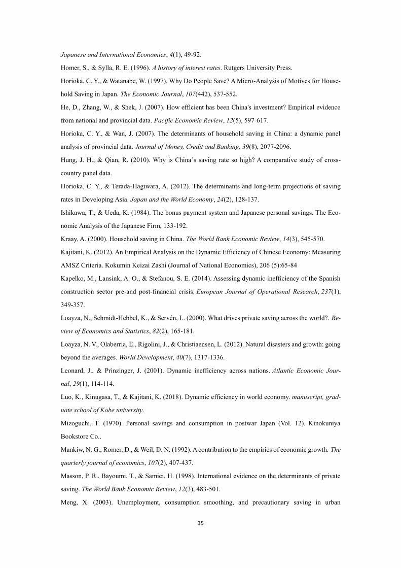
In this subsection, we refer to the estimates in Luo et al. (2018)—our earlier work re-

garding the 21st century dynamic efficiency of the world’s top-30 largest nations ranked by

GDP and of other OECD participants3—summarized in Table 14. The AMSZ criterion applied

in the estimates contends that dynamic efficiency can be assessed by observing the cash flow

generated in the production sector. To be precise, an economy is deemed to be dynamically

inefficient (overaccumulated) if the total capital investment overwhelms the gross capital gains,

and vice versa. For comparability, in Table 1, the efficiency is expressed as the proportion of

the cash flow in GDP.

It should be noted that, as many studies have suggested (e.g., Abel et al. 1989; Ahn 2003;

3 Among the top-30 nations, we drop the observations of Indonesia, Saudi Arabia, Ar-

gentina, Thailand, Iran, and United Arab Emirates, as official statistics on these nations are not

suitable for measuring the criterion.

4 The estimates are directly taken from Luo et al. (2018). Interested readers can refer to

this paper for a comprehensive survey on the assessment of dynamic efficiency.

6

Geerolf 2013; Luo et al. 2018), although the AMSZ criterion has various advantages over other

approaches, this method suffers from substantial statistical limitations, which may eventually

cause an upward bias in the returns to capital. In this regard, estimates without bias correction

can provide overoptimistic results about the magnitude of overaccumulation. As Table 1 implies,

however, it turns out that even the non-corrected estimates suffice to verify China’s over-saving

status. Among the observations presented in the table, China has undoubtedly encountered the

most severe problem of overaccumulation in the past decade. It is tempting to conclude that if

overaccumulation does exist and only exists in a certain country, China would be the one.

2.3 An analytical stance in viewing saving issues

Before proceeding, we would like to clarify why it is crucial for our case study to take a

stance on China’s overaccumulation status. In the saving literature, economists usually refer to

traditional macroeconomic theories that emphasize the importance of saving and investment—

regarding saving as the source and prime engine for economic development5. Typical examples

are the Lewis model and the first and second “demographic dividend” hypotheses, which have

well formulated the growth impact of saving. Moreover, there is ample evidence revealing the

positive correlation between saving (investment) and economic growth, focused explicitly on

the developing world (e.g., Mankiw et al. 1992). At the household level, as a part of private

assets, saving signals an improvement in the standard of living by moving beyond subsistence

consumption. Simply put, it is tempting to regard saving as a completely positive element and

5 That is, saving is a major source for corporate investments in plants and equipment

needed to promote the productive capacity of the aggregate economy, and the enhanced income

growth feeds back through stimulating household saving.

7

thus overlook the “evil” side of it.

However, there is much to be discussed about the internal threats that overaccumulation

might bring about, not to mention its adverse external impacts. First, if an economy has over-

accumulated capital such that the interest rate (r) falls below the economic growth rate (g),

maintaining the market equilibrium will require more investment (gK) than the economy actu-

ally produces (rK) (Fama and French, 2002; Weil, 2008). Second, capital saturation (g＞r) ren-

ders additional investment pointless since the capital stock has exceeded the optimal amount

for maximizing social consumption. In this sense, oversaving is a practice of “extravagance”

(Luo et al. 2018). According to the OECD balance sheets, whereas the capital formation ratio

(GCF/GDP) of China increased steadily from 35% to 46% over the 1990–2015 period, its con-

sumption ratio (FCE/GDP) has declined sharply from 64% to 52% during the same period. In

other words, China’s capital-extensive growth pattern—reliant on the excessive investment and

exports—has never achieved proper welfare gains (socially inefficient). Third, overaccumula-

tion always triggers speculative bubbles and income inequality, which can jeopardize the mar-

ket effectiveness and social stability.

While it is almost impossible to reach a definitive conclusion on the overall impact of

overaccumulation, we believe that this growth model is pathological and unsustainable. For

Chinese policymakers, it will be mostly beneficial to encourage consumption, increase the in-

terest rates, and eliminate the idle capital, rather than sticking to the saving-promotion strategy.

From this vantage point, in examining China’s saving behavior, factors regarded as pos-

itive elements (i.e., the saving-promoting factors) might have negative repercussions on China’s

economic performance because they have aggravated the problem of capital overaccumulation.

8

Similarly, those regarded as negative factors (i.e., the saving-inhibiting factors), might have

virtually reduced the idle capital and thus served as remedies for the overaccumulation problem.

An analytical stance is of utmost importance in diverse research topics: merely identifying the

driving forces of a certain phenomenon is not sufficient; we need to understand how these fac-

tors can contribute to a better economic status. Although the position we take does not influence

the empirical assessments, it does, to a large extent, change the way we interpret and make use

of the statistical inferences—which might turn out to be contradictory to the common view and

have important implication for China’s policy designs.

9

3. Data and empirical strategy

3.1 Data

The analysis is based on China’s panel dataset comprising 30 administrative units (i.e.,

provinces, autonomous regions, or municipalities) divided into rural and urban samples over

the 1995–2015 period—a time span covering the rapid evolution of China’s capital accumula-

tion. All the variables are taken or constructed directly from Chinese statistics yearbooks, pop-

ulation and employment statistics yearbooks, and finance and banking yearbooks, published by

the National Bureau of Statistics of China.

One drawback of the dataset is that some indicators are not available for certain admin-

istrative units over particular periods. For instance, we drop the unit “Tibet” owing to its severe

inconsistency and missing values; Chongqing city became independent from Sichuan province

in 1997, and thus some figures are not recorded until 1997; in addition, data on a handful of the

major indicators are available only at the provincial level, making it difficult to distinguish

between the separate impacts on rural and urban households. However, this limitation can be

overcome by altering the definition and interpretation of variables, as discussed in the later

section. For completeness, the descriptive statistics and pairwise correlation matrix are shown

in Appendix, which provide basic information on incorporated variables.

3.2 Econometric procedure

To identify a broader range of determinants, rather than adhering to structural-form ap-

proaches, we prefer a reduced-form linear specification that helps to arrive at straightforward

empirical regularities.

10

S𝑖,𝑡 = β1S𝑖,𝑡−1 + β2X𝑖,𝑡 + 𝛿𝑡 + 𝜇𝑖 + 휀𝑖,𝑡 (3.1)

The specification outlined above is a standard regression designed to assess the determi-

nants of household saving based on panel data. The subscripts t and i represent the time period

and province, respectively; S denotes the household saving rate, where the coefficient

β1 should be less than unity; X is the set of explanatory variables; δ and μ represent the unob-

servable time- and province-specific effects, respectively; ε is the disturbance term.

We pay careful attention to the endogeneity and heterogeneity considerations—the main

challenges confronting the empirical assessments of saving behaviors. In line with the previous

literature6, we utilize the GMM estimator (Generalized-Method-of-Moment7), which is an an-

alytically sound and empirically feasible approach to investigate dynamic problems.

This method is superior to other approaches in several aspects. First, for the time-series

consideration, the GMM framework allows for dynamic specification by incorporating lag

terms of dependent variables. In the saving literature, a lagged saving rate represents the inertia

and persistence of saving behaviors, which can explain and account for a notable proportion of

variations in the variable. In this setting, we retain the time-series information rather than dis-

torting it by arbitrarily taking the average of variables over certain time spans.

Second, the Difference-GMM estimator controls for the time-invariant effects (i.e., the

province-specific effects), which constitute 35% of the saving variations in the selected dataset

6 We follow studies such as Loayza et al. (2000, 2012), Schrooten and Stephan (2005),

Horioka and Wang (2007), Hung and Qian (2010), and Nabar (2011) in this regard.

7 See Arellano and Bond (1991) and Arellano and Bover (1995) for a full description of

this technique.

11

(see Appendix). The first-difference process can mitigate the bias stemming from the heteroge-

neity in cross-regional observations. That is, after accounting for the time trends, this method

eliminates the overall unobservable effects in the regression.

∆S𝑖,𝑡 = β1∗∆S𝑖,𝑡−1 + β2

∗ ∆X𝑖,𝑡 + ∆휀𝑖,𝑡 (3.2)

Third, macroeconometric assessments are often plagued by the limited availability and

poor reliability of exogenous instruments in coping with the endogeneity concern. To address

this problem, the Difference-GMM estimators exploit the internal instruments—the lag values

of explanatory variables—to steer clear of the simultaneous and reverse causalities, and thus

control for the overall endogeneity. Provided that the error term is serially uncorrelated and that

the regressors are by construction weakly exogenous, the following moment conditions are used

to calculate the consistent Difference-GMM estimators.

E[S𝑖,𝑡−𝑘 ∙ ∆ε𝑖,𝑡] = 0 for k ≥ 2; k = 3, … , T (3.3)

E[X𝑖,𝑡−𝑘 ∙ ∆ε𝑖,𝑡] = 0 for k ≥ 2; k = 3, … , T (3.4)

3.3 Empirical issues regarding the GMM estimators

Similar to the conventional IV method, the GMM estimators pivot critically on the va-

lidity of instrument variables. To this question, we perform two specification tests. First, the

Hansen test is used to inspect the overidentification restriction on instrument variables. Failure

to reject the null hypothesis lends credence to the weak exogeneity and joint validity of the

internal instruments. Second, the first- and second-order serial correlation tests are used. Failure

to reject the second and success in rejecting the first8 verifies the random-walk process in AR

8 By construction (i.e., the first-difference procedure), the error term (∆휀𝑖,𝑡) is expected

to be correlated with the dependent variable (∆S𝑖,𝑡), which leads to a rejection in the first-order

12

(2), which supports the overall reliability of the GMM estimators on the basis of dynamic mo-

ment conditions.

Considering China’s remarkable economic progress, it is not surprising that many em-

pirical attempts have been made to explain its extraordinarily high saving rates. Nevertheless,

the literature tends to be limited in several respects to which we refer and propose our solutions

as below.

1. According to Blundell and Bond (1998), the internal instruments employed in the first-

difference regression are not likely to serve as proper instruments. As critiqued by other authors9,

the Difference-GMM method underemphasizes the time-invariant effect and it is inclined to

over-difference the specification. To overcome this limitation, we use the System-GMM

method advanced by Blundell and Bond (1998), which combines the difference and level equa-

tions into one system to control for the potential bias.

The strategy is, on the basis of the Difference-GMM estimator, the system incorporates

the lagged differences of variables as internal instruments for level equations. These are valid

instruments if the correlation between each variable and the province-specific effect is constant

over time (equation 3.5).

E[X𝑖,𝑡+𝑝 ∙ μ𝑖] = E[X𝑖,𝑡+𝑞 ∙ μ𝑖] and E[S𝑖,𝑡+𝑝 ∙ μ𝑖] = E[S𝑖,𝑡+𝑞 ∙ μ𝑖] for all 𝑝 and 𝑞 (3.5)

In the System-GMM estimator, the above assumptions are formulated into additional

serial correlation test. 9 For instance, Alonso-Borrego and Arellano (1999) suggest that if the sample size is

limited and the variables are highly persistent over time, the internal instruments exploited in

the Difference-GMM method can be weak instruments, which jeopardize the asymptotic sta-

bility and result in estimation bias.

13

moment conditions (equation 3.6), which can contribute to more accurate and efficient assess-

ments.

E[∆X𝑖 ∙ μ𝑖] = 0 and E[∆S𝑖 ∙ μ𝑖] = 0 (3.6)

2. Windmeijer (2005) suggests that due to the uncontrolled heterogeneity and tenuous

restriction on the weight matrix, the conventional one-step GMM estimator tends to ineffi-

ciently specify the weight matrix in computing coefficient estimates. This limitation impairs

the reliability of the overidentification test, thus leading to a corresponding upward bias in the

statistical significance, especially for finite-sample estimations. However, Arellano and Bond

(1991) and Bond (2002) argue that the one-step method is a reasonable choice to reduce the

overfitting bias in small-sample estimations, and the efficiency gains from using the two-step

version are very modest. Considering that the sample size in question is neither small nor suf-

ficiently large, we incorporate the two-step System-GMM estimator proposed by Arellano and

Bond (1991) and Arellano and Bover (1995), and compare its estimates with the one-step ver-

sion to test the robustness.

3. Roodman (2007) and Loayza et al. (2012) suggest that utilizing smaller lag lengths to

derive a limited set of moment conditions helps to avoid the overfitting bias in conducting the

GMM estimations. Furthermore, it is worth nothing that the GMM estimates are rather sensitive

to the choices of the lag period (Tauchen 1986). For overall robustness and transparency, we

perform consistency tests by experimenting different lag choices (from 2-3 to 2-5) on the major

explanatory variables, combined with the command “robust” to mitigate the heteroscedasticity

in computing standard errors.

14

4. In the System-GMM estimations, when the available time span and the set of explan-

atory variables are adequate, the introduction of internal instruments usually causes a surge in

the number of instruments and leads to a severe overidentification bias. To address this problem,

we adopt the command “collapse” developed by Bond (2002) to restrict the size of potential

instruments. In addition, following Loayza et al. (2000) and Wang et al. (2012), we utilize the

command “noconst”10 to eliminate the constant term (i.e., the time trend in the first-difference

regression) that overlaps with the saving persistence in question. Neglecting this problem can

lead to an upward bias in the estimated saving propensity.

5. As Masson et al. (1998), Loayza et al. (2000), and Kraay (2000) put it, empirical as-

sessments regarding saving behaviors are particularly sensitive to the choices of econometric

techniques, variables, and samples. In the current study, perhaps the most important concern in

this regard is the huge conceptual difference between China’s urban and rural household sur-

veys. Accordingly, it is desirable to disaggregate the estimations under different scenarios and

examine the rural and urban samples separately to highlight the intra-provincial differentials.

Moreover, as the existing literature has made clear11, the conventional determinants of saving

behaviors have very limited power in explaining the exceptionally high saving rates in China.

There is an urgent need to exploit a wider range of variables—the newly formed, country-spe-

cific, and less standard determinants—to resolve the conundrum.

10 Estimates are robust to the choices of commands, but these are not discussed here due

to space limitation. 11 See, for example, Kraay (2000), Horioka and Wan (2007), Hung and Qian (2010), Wei

and Wang (2011), and Horioka and Terada-Hagiwara (2012) in this regard.

15

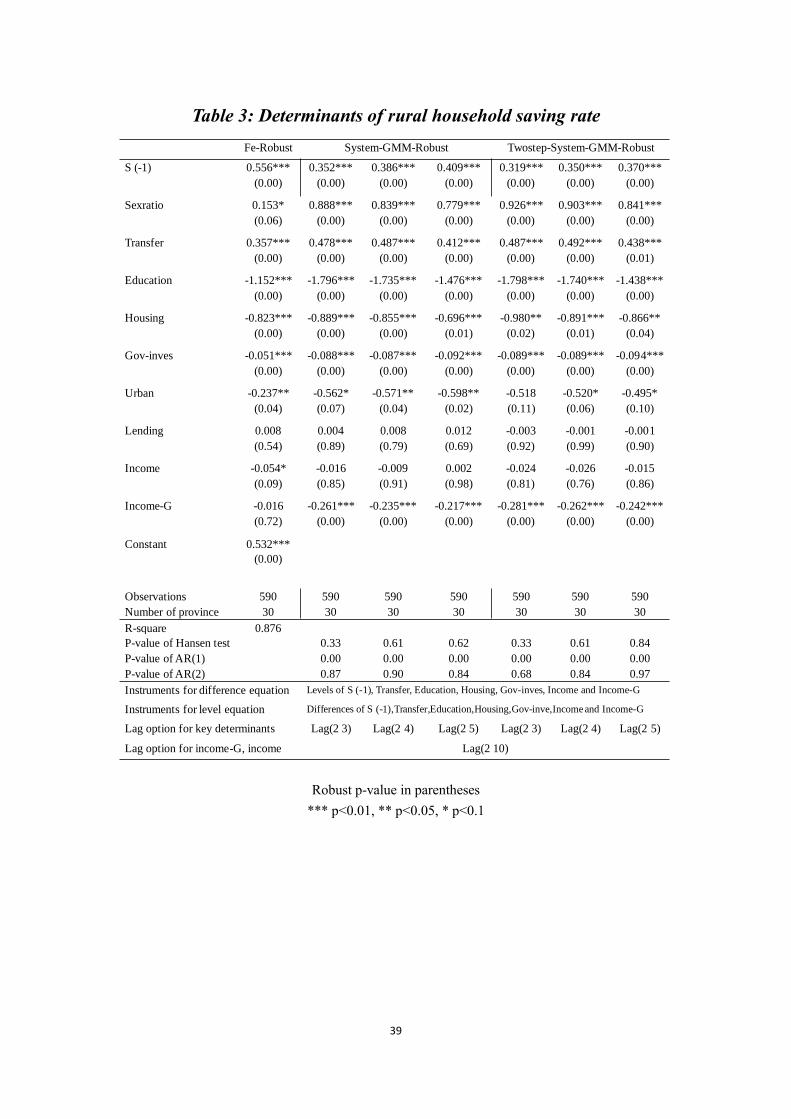
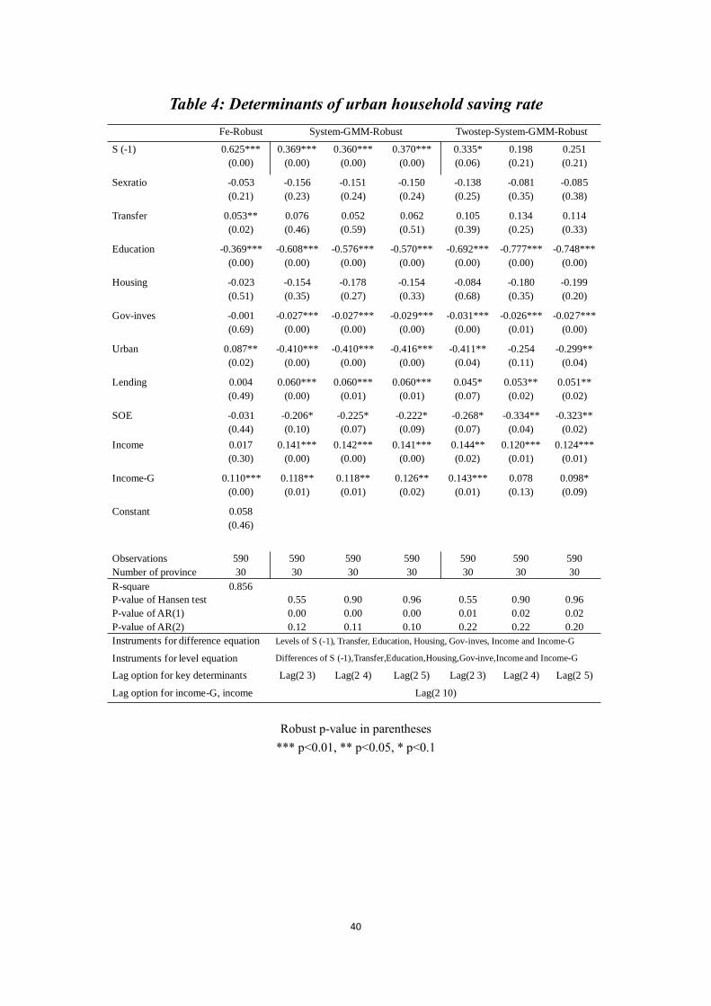
4. Specification test, result, and interpretation

In this section, to allow concise expressions, for each variable, we combine its definition,

estimate, and interpretation in order. Tables 3 and 4 demonstrate the estimations for rural and

urban samples, respectively. For overall comparability, both parts use the same modeling strat-

egy. It is reassuring that the Hansen and serial correlation tests support the empirical validity of

the regressions, and the estimates are fairly robust to different lag choices and econometric

methods—the Fixed-effect12(column 1), one-step (columns 2–4), and two-step System-GMM

approaches (columns 5–7). The parameters obtained in both parts are theoretically justifiable,

and will be discussed in detail. We also conducted the consistency tests, and the results are

summarized in Tables 5 and 6. These exercises suggest that with the inclusion of additional

covariates, major determinants retain their statistical significance as well as coefficient signs.

In the estimations, we include the conventional income-related determinants as control

variables, and focus on the less standard determinants, which are essentially the predominant

drivers of Chinese household saving. As typical demographic variables, the sex ratio, urbani-

zation ratio, and share of SOE employees are assumed to be strictly exogenous. The total bank

lending is also considered to be exogenous. Other variables are deemed to be endogenous or

predetermined and thus correlated with the error term—the primary reason to utilize the GMM

estimator as the baseline specification. In the estimations, we also look into the common mis-

understandings in the use of several proxy variables, and make attempts to present proper def-

inition and interpretation on each variable.

12 We incorporated the within estimator (fixed-effect) to test the robustness and to obtain

the overall explanatory power (i.e., the R-squared, which is unobservable in the GMM estima-

tions) of the preferred explanatory variables.

16

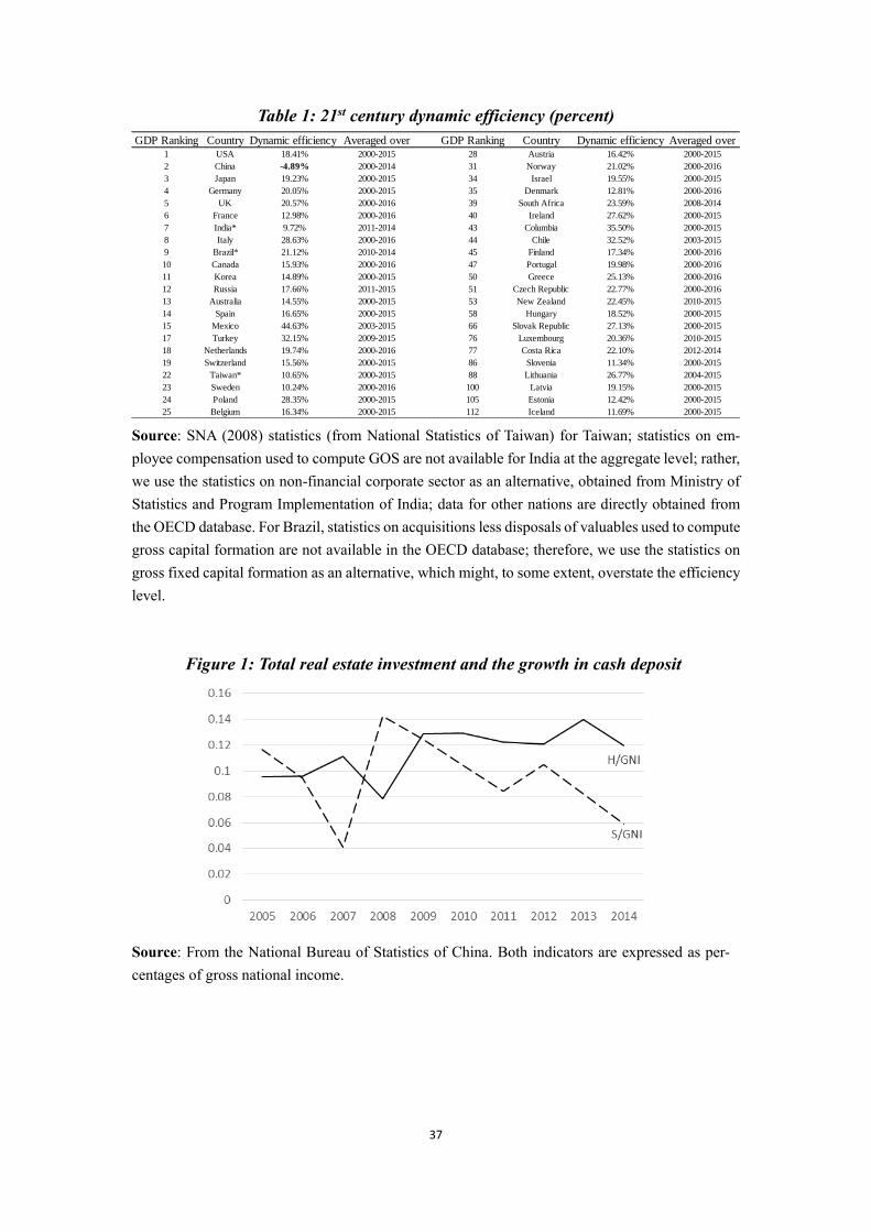
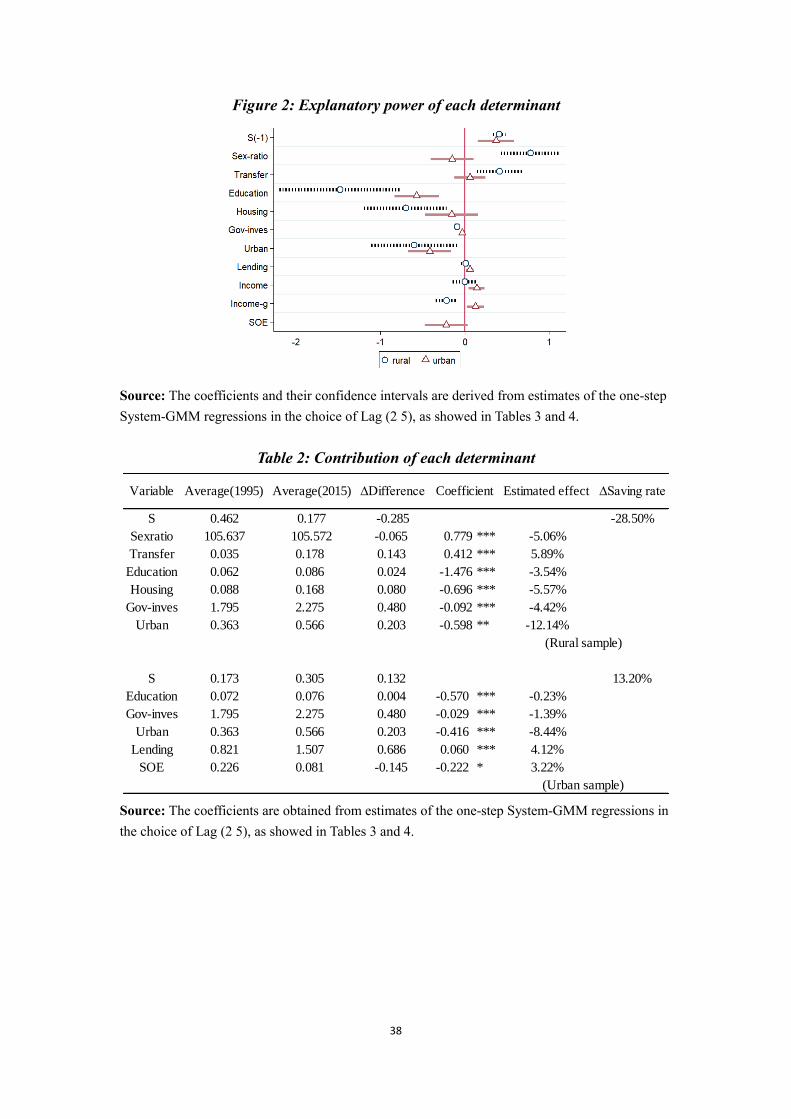
To draw a comprehensive picture of the results, Figure 2 summarizes the estimated coef-

ficient (the marginal effect) and confidence interval of each variable; Table 2 displays the esti-

mated long-term contribution of each variable to the variations in saving rates—the larger the

parameter and higher the deviation, the more pronounced impacts on saving. Accordingly, the

education and housing expenses, transfer income, government investment, urbanization ratio,

and sex ratio are deemed to be the main driving forces of rural household saving. In turn, the

education expenses, government investment, bank lending, urbanization ratio, and share of

SOE employees are considered to be highly influential on urban household saving.

4.1 Dependent variable

Household saving rate. Household saving rate (S/Y) is calculated in a traditional method

as the ratio of household saving (i.e., the difference between income and total expenditure) to

household disposable income.

Saving rates in China have been higher than any other nation since 1995. They vary

across space and over time, with thumping long-term differences and non-trivial short-term

fluctuations. The rural household saving rate as a provincial average decreased sharply from

46.2% to 17.7% during 1995–2015, whereas the urban counterpart increased from 17.3% to

30.5% over the same period. As the subject matter of the study, we will unveil the promising

determinants of Chinese household savings in the following part.

4.2 Explanatory variables

Inertia and persistence. According to the estimates, the one-year lag of saving rate has

a positive and significant impact on the current saving rate, which confirms the non-negligible

17

time-series contribution from the saving persistence. The coefficients range from 0.32 to 0.56

for rural samples and from 0.34 to 0.63 for urban samples (statistically significant estimates

only), implying that the long-run effect of saving inertia is 1.47 to 2.70 times the respective

short-run effect (if these effects persist over time), which are lower than the findings of previous

studies on saving persistence13.

This insight suggests that China’s “saving glut” is not necessarily a consequence of its

“high” propensity to save—the Confucian heritage: diligence and thrifty—an idea frequently

picked up by the media and anecdotal literature. Moreover, it is apparent that there is no notice-

able disparity between rural and urban saving inertias. Accordingly, the saving persistence is

neither a critical explanation for the extraordinary high saving rates in China, nor is it an over-

riding force for the urban saving rate to surpass the rural counterpart in the past decade.

Sex ratio. Sex ratio is calculated as the number of males per 100 females (in total popu-

lation). Since the data for this indicator is only available at the provincial level14, it is employed

in both the rural and urban estimations as a policy instrument.

In the past decades, the world has witnessed the efforts made by China in limiting its

population. China’s One Child Policy and Family Planning Program have been subject to much

debate (e.g., Modigliani and Cao 2004; Horioka and Wan 2007; Ma and Yi 2010; Nabar 2011).

13 We refer to previous studies such as Such as Loayza et al. (2000), Schrooten and

Stephan (2005), Horioka and Wang (2007), Hung and Qian (2010), and Nabar (2011), in which

the estimated coefficients range from 0.3 to 0.8. 14 An alternative is the “household sex ratio”. Information on this indicator is available

for both rural and urban samples for the period of 2003–2015. However, we do not use this

indicator owing to substantial outliers and problematic observations in the statistics.

18

The literature has clarified that a lower fertility rate driven by the population policies has re-

lieved the household burden and led to declines in within-family insurance, resulting in higher

savings, which is consistent with the life-cycle hypothesis. This is, however, a narrow reading.

Note that China’s sex ratio at birth is never “natural” (over 1.2 boys per girl in the early 2000s,

see Wei and Zhang 2011); what stabilized the sex ratio of the total population (around 1.06

males per female during the 1995–2015 period), are the family planning policies and re-

strictions on sex-selective abortion—which have introduced profound changes in household

decisions.

In the context of the Chinese traditional culture, men ought to play the dominant role

whereas women were expected to be their subordinates. This kind of feudal ethic usually un-

dermines females’ saving motives. Wei and Zhang (2011) find that parents with a son raise their

saving in a competitive manner in order to improve their son’s relative attractiveness for mar-

riage. This finding is supported by Hung and Qian (2010), but is in contrast with Banerjee et

al.’s (2010) finding that Chinese households with a daughter tend to save more for the precau-

tionary motive. In a macro-based analysis, Nabar (2011) does not find any strong statistical

relevance in favor of these hypotheses. Intuitively speaking, the so-called feudal ethic is more

entrenched in the less-developed regions; therefore, rural residents will respond more strongly

to the fluctuations in sex ratio by reallocating their time resources (i.e., saving and consump-

tion).

In line with our expectations, the estimates suggest that rural residents react more

strongly to the changing sex ratios. As a rough evaluation, the declining sex ratio has a consid-

erable negative effect (-5%) on the rural household saving rate. Although China’s population

19

policies have been subject to much criticism for moral considerations and the pessimism of

economic slowdown, they have been serving as a remedy for the excess saving problem in

China’s rural districts.

Transfer income ratio. Transfer income ratio is calculated as the share of total transfer

income in the household disposable income.

The variable represents the inter-family transfers, such as bequests, alimony, and gifts

inter vivos15. Conceptually, if all the family members are self-sufficient and having available

financial approaches, there might be little “deep reason” behind the transfer they received.

However, as a result of the frayed social safety net and the underdeveloped financial

system in less developed regions, inter-family transfer might serve as the primary vehicle for

rural households to guard against risks. Mainstream theories regard the altruistic transfer as a

tool to help smooth the consumption of other people. In this sense, if motivated by altruistic

spirit, transfer income is compensatory and usually impairs receivers’ motive of pension saving,

which lowers the household saving rate. From an alternative perspective, as O’Connell and

Zeldes (1993) and McGarry (2016) suggest, when individuals plan to dissave, whether inten-

tionally or unintentionally, they release a signal of greater need for external aid to maintain and

smooth their current consumption. Simply put, there is a reverse causality from recipient’s well-

being (e.g., deposit) to the transfer received—when one dissaves, one receives more. Besides,

a well-known theory is that parents regard children as a substitute means for asset and buffer

15 In fact, the variable also includes government transfers such as social security and

pension. In this study, taking into account the underdevelopment of China’s pension systems

and safety nets, we primarily focus on the inter-family transfer and its effect on saving.

20

stock, and they conduct transfers in exchange for old age support (e.g., Cox 1987). This can be

captured by the inter-family transfer if parents and their children belong to different households.

Overall, both the altruistic and “selfish” hypotheses predict either no or a negative correlation

between the transfer income and saving rate.

In contrast to the conjecture that the transfer income is either an exogenous income or a

saving-inimical element, the estimates demonstrate a significant and positive impact on rural

household saving rate. The derived coefficients indicate that receivers’ marginal propensity to

consume out of the transfer is relatively small. Precisely, rural residents will save one-half of

the transfer they received, rather than adhering to the general pattern (average saving rate is

around 25%). This insight seems to be a considerable departure from the mainstream theories,

since it suggests that the transfer is not meant to be consumed, but to be preserved.

There is some early but indirect evidence on the phenomenon16. As predicted by Barro’s

dynastic altruism model, a plausible explanation is that transfer income might have a Ricardian

effect on household saving17. That is, receivers perceive that the transfer is a “loan” that better

be reimbursed in the future, rather than a kind of temporary income capable of being dispensed

discretionarily. A more comprehensive interpretation is that, in line with the permanent income

hypothesis, due to the inferior rural welfare benefits, rural residents tend to save more out of

their transitory income (e.g., the inter-family transfer). Another likely explanation, which lends

support to the rule-of-thumb hypothesis, is that low-income individuals tend to save a half or

16 For instance, Mizoguchi (1970), Ishikawa and Ueda (1984), Meng (2003), and Raval-

lion and Chen (2005) have found that the marginal propensity to save out of regular income can

be lower than that out of temporary income (such as bonus and other lumpsum transfers);

Hayashi (1986) infers that the increase in annuities did not lead to a higher consumption of the

elderly in Japan. 17 The argument usually refers not to bequests, but to the “gifts” inter vivos.

21

two-third of their temporary income.

Given that the transfer ratio increases from 3.5% to 17.8% over the observation period,

it has a tremendous promoting effect on the rural household saving rate (by 5.8%). Whereas

discerning the effect’s mechanism is beyond the competence of the data at disposal, as con-

firmed by the estimates, the unclear mechanism plays an equilibrating role in moderating the

declining rural saving rate, which has aggravated the problem of surplus saving.

Housing and education expenses. This variable is calculated as the shares of housing

and education expenses in disposable income.

Since the initiation of the housing stock privatization in the 1990s, China’s real estate

market has begun to expand at an unprecedented rate. As China entered the 21st century with a

flexible monetary policy and incomplete restriction on property purchase, accompanied by bur-

geoning inflation and rapid economic growth, the real estate market began to experience an

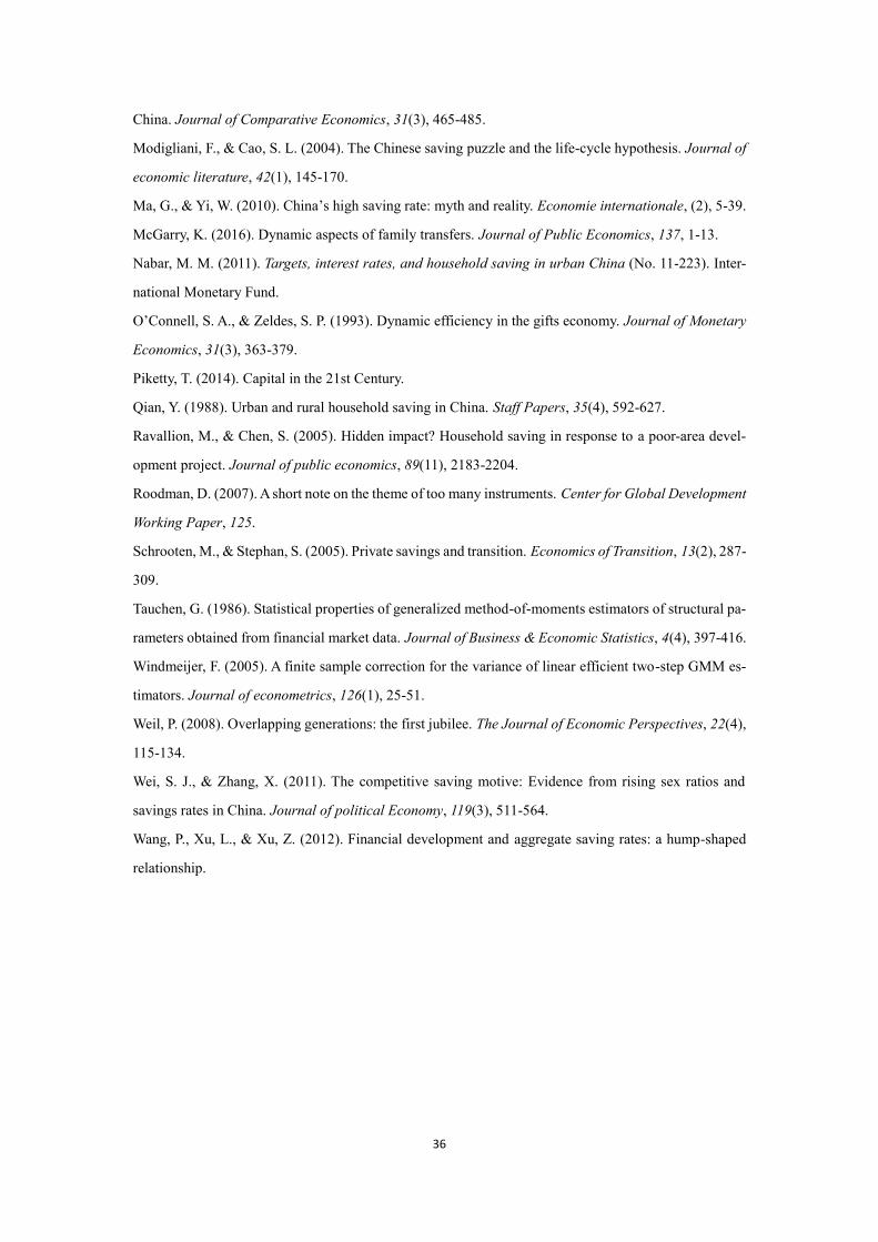
overwhelming expansion, which shows no sign of decline over the past decade. Figure 1 plots

the total real estate investment against the growth in national cash deposit for 2005–2015. At a

first glance, there is an obvious substitution relationship between the investment and saving

accumulation at the aggregate level.

On the other hand, China began to pursue the Higher Education Reform in 1999, with

the system of nine-year compulsory education being implemented in earnest. The increase in

education funding has succeeded in relieving households from the burden of education expendi-

ture. Moreover, thanks to the decreasing fertility rate triggered by the population policies, in

22

2015, the share of education expense in the household disposable income expressed as the pro-

vincial average reached 8.0%, which well reflects China’s light educational burden by interna-

tional standards.

To capture the variations in household expenditure, rather than employing the indices of

quantity and price, which are highly volatile and often unavailable, we choose a direct specifi-

cation—the share of each expenditure in household income. While this approach is empirically

feasible, it should be noted that savings as well as other expenses are part of the household

budget; thus, there is always a neutral crowding-out relationship between any two expenditures

in the estimations18—an empirical issue often overlooked by the previous literature. In the re-

gressions, negative signs of coefficients only suggest that the expenses offset saving when

households have a limited income. That is, coefficients with a value above -1 (in real numbers,

hereafter) do not imply a substitution effect on saving. On the contrary, the opposite (a comple-

mentary effect) might be true.

Whereas the characterization is not rigorous and deserves further investigation, it is a

useful first step to identify the empirical regularity between saving and household expenditure.

Precisely, if the expenditure is a substitute for saving, its coefficient is expected to be lower

than -1, since the crowding-out effect alone can lead to a coefficient of -1; if the expenditure

and saving experience a joint demand, the coefficient of expenditure should be above -1; if the

complementary relationship is strong, the coefficient might even obtain positive values.

As claimed by the estimates, the coefficients of education expense range from -1.80 to -

18 Saving is a residual concept. That is, Saving/Income = 1 - (Expenses/Income). In this

sense, the crowding-out effect alone leads to an estimated coefficient of -1.

23

1.44 for rural samples, and from -0.78 to -0.57 for urban samples. Accordingly, education ex-

penses have a significant substitution effect on rural household saving but a complementary

effect on urban household saving. On the other hand, the housing expense has a moderate com-

plementary effect on rural saving, whereas the coefficients in the urban estimation are statisti-

cally insignificant, implying a strong complementary effect of housing expense on urban saving.

City dwellers usually spend much more than rural residents on both dimensions. However,

the estimates point toward a significant substitution relationship between the education expense

and rural saving. This implies that rural residents have to break into their saving to finance the

education expenditure, whereas the negative impact on urban saving is somewhat muted, even

though urban residents are confronting much higher charges. In a similar vein, the estimates

suggest that the home purchase of urban residents is not largely financed out of their saving; at

least, the rising housing expense of urban households does not seem to influence their saving

rate. This insight is very similar to Japan’s case that a high saving rate of the young population

triggered by the surging housing prices did not translate into higher aggregate saving (Hayashi

1986; Horioka and Watanabe 1997). This is in contrast to the literature, which regards the sav-

ing motivations for homeownerships and life-cycle events as contributors to higher national

saving rate (e.g., Chamon and Prasad 2010; Nabar 2011).

The contrast is even sharper when the overaccumulation problem is being considered. In

the past decade, the world faced a common threat posed by real estate bubbles (e.g., the Lehman

shock). However, rational bubbles can help absorb the excess saving in many ways (e.g., in-

ducing transfers from the young to the old). In this sense, to some extent, asset bubbles have

attenuated China’s overaccumulation and improved its efficiency status. As the estimates have

24

quantified, the increasing housing expense in the past 20 years has contributed to a notable

deduction (-5.6%) in the rural household saving rate.

On the other hand, China’s education reform has become one of the most successful pol-

icy designs. The highly subsidized education funding has lifted millions out of illiteracy and

helped the rural population pursue college education. From a different perspective, the favora-

ble education system has a compensating effect on household saving. Over the 2000–2012 pe-

riod, the diminishing educational burden has stimulated the excess savings of rural and urban

households by 4% and 3%, respectively, which has worsened the over-saving problem in China.

Government investment ratio. This variable is calculated as the ratio of public invest-

ment to financial revenue. Since information on this indicator is only available at the provincial

level, we employ it in both rural and urban estimations.

Following the existing literature (Masson et al. 1998; Loayza et al. 2000; Hung and Qian

2010), we examine the effect of public investment on household saving from two perspectives.

First, we discuss the efficiency of government investment: if the investment is ineffective

(for example, a pointless war at a huge cost which generates no return), it is likely to reduce the

resources available to the private sector and thus decrease the saving accumulation of house-

holds.

Second, we examine the effect from the perspective of Ricardian equivalence: if typical

agents are rational and forward-looking, fiscal policies will have a crowding-out effect on

household portfolios. That is, if individuals are capable of anticipating that the deficit (surplus)

25

in budget balance will only lead to future increases (reductions) in their tax liabilities, any ex-

pansion (reduction) in government spending can be completely offset by increases (decreases)

in household saving. Although economists today have reached a consensus that full rationality

and complete equivalence are empirically irrelevant (e.g., Bernheim 1987; Elmendorf and

Mankiw 1999), intuitively speaking, government behaviors always influence households’ sav-

ing decisions. In this regard, we expect to capture a partial Ricardian effect—non-negative co-

efficients in the regressions.

As reported by the estimates, public investment has significant and negative impacts on

rural and urban household savings, which reject the Ricardian hypothesis. The estimated coef-

ficients suggest that a 1% increase in the investment ratio is associated with modest decreases

of -0.09% and -0.03% in rural and urban household savings, respectively, implying that China’s

public investment is urban-favoring since it is less detrimental to the process of urban capital

accumulation.

The sizeof the Chinese government and its fiscal deficit have been maintaining high lev-

els, with the investment ratio at the provincial average increasing steadily from 1.795 to 2.275

in the 1995–2015 period. As a consensus view, lower government involvement promotes mar-

ket efficiency and encourages innovation. The phasing out of government participation and the

introduction of competitive mechanisms are considered to be the key methods of constructing

an ideal society. On the other hand, over the past 20 years, the increasing public investment has

contributed to considerable reductions in rural and urban household saving rates (by -4.4% and

-1.4%, respectively), which have counteracted the over-saving problem.

26

Urbanization ratio. This variable is calculated as the share of urban population in the

total population.

This is not the first study to utilize the urbanization ratio as a saving determinant (for

example, see Loayza et al. 2000; Hung and Qian 2010). Part of the literature considers that

rapid urbanization adds to uncertainty and motivates the precautionary demand for saving. Yet,

some researchers argue that urbanization is usually accompanied by financial liberations, which

relieve the borrowing constraints and thus lower corporate and private savings, supported by

the fact that industrial countries always have lower national saving rates. In the above cases,

the ratio serves as a proxy for the level of urbanization construction. This is, in our view, a

rather far-fetched interpretation.

A prime reason is that, for China, the ratio depends crucially on its administrative divi-

sions19. In cross-section comparisons, higher urbanization ratios do not necessarily imply higher

levels of urbanization construction. On the other hand, is time-series comparison feasible to

reflect the urbanization process and urban population growth (the natural birth) within a prov-

ince? The answer is probably no. In China, the life expectancy of the urban population is higher,

but the growth effect is roughly offset by the rural-urban divergence in fertility rates. In sum-

mary, the ratio is not a proper proxy for the level of urbanization construction. Rather, it is a

satisfying proxy for the rural-urban population movement in the dual economy, which explicitly

accounts for the ongoing phenomenon of “Rural Hollowing.”20

19 A typical example is the Hebei province. The province is known for its heavy indus-

tries and high level of urbanization construction; however, its urbanization ratio was merely

0.50 in 2015, which is the lowest among all administrative units. 20 To be clear, the variable also reflects the impacts from other dimensions, for instance,

the effect of financial development. We control for these confounding effects by incorporating

explanatory variables such as the bank lending and income-related determinants, discussed

27

The main content of the rural-urban migration—prime-age adults at their peak earning

years—is also the main force in saving accumulation. Accordingly, it is plausible to expect a

negative impact of the work force movement on rural household saving, and a positive impact

on urban saving since the “new-comers” (rural labor) presumably have a higher propensity to

save. According to the estimates, the impacts are negative and statistically significant for both

rural and urban samples. The negative coefficient in the urban sample suggests that, on average,

the newcomers are not able to catch up with the level of urban saving, which in turn has brought

down the urban household saving rate, probably due to the fact that migrant workers usually

earn less while confronting higher living expenses in urban regions.

The Rural Hollowing phenomenon has so far been a common challenge worldwide. It

has aggravated the shortage of rural labor resources, worsened the problem of the aging society

in the countryside, and caused population explosion and soaring prices in metropolitan areas.

From an alternative perspective, as a rough evaluation, this population movement has contrib-

uted to saving reductions of rural and urban households (by 12.1% and 8.4%, respectively) over

the past two decades. In this sense, other factors seem to have a little role compared with the

phenomenon in regulating excess savings. Thus, this phenomenon is primarily responsible for

the decreasing rural household saving, and has been serving as the most potent weapon against

the overaccumulation problem in China.

Total bank lending. This variable is calculated as the ratio of total bank lending to pro-

vincial nominal GDP. Since information on this indicator is only available at the provincial

fully below.

28

level, we employ it in both estimations.

Numerous indicators have been used in the literature to measure financial depth and fi-

nancial liberalization. However, rather than using conventional figures (such as the M2 and

M3)—which are highly associated with the economic status (such as inflation) and the corre-

sponding financial policies, and thus could contaminate the statistical inference—we adopt the

indicator of total bank lending to account for the credit provision21.

Other things equal, a greater availability of consumer credits usually reduces household

saving, since there is no reason for individuals to save via borrowing. As some critics believe,

however, there is a widespread priority order in China’s banking system, wherein bank loans

are provided preferentially to local governments and SOEs. Private enterprises suffer discrim-

ination regarding the provision of bank loans because of their relatively small scale and limited

sources of repayment. Consequently, in preparation for bad times, China’s private sectors tend

to retain a large proportion of their earnings, and they usually finance their expenditure from

the unrecorded contributions of workers. This “hidden” rule applies equally to the case of pri-

vate borrowing. That is, the priority order favors upper-income citizens in receiving preferential

treatment, whereas rural households seem least likely to benefit from the impressive progress

in China’s financial liberation over the past decade.

Accordingly, an increase in bank lending does not necessarily reduce savings. Rather, it

depends on who/which sector receives the expanding credits. Precisely, if the low-income group

acquires most of the credits, bank lending will lower the household saving rate; on the other

hand, if the credits are largely obtained by the high-income population and large enterprises,

21 The private credit is a more direct measure; however, information on this indicator is

not available for the overall sample period.

29

the expansion in bank lending might even exhibit a positive impact on saving accumulation,

because the richest always saves the most22.

In agreement with the intuition, the estimates confirm the so-called priority order, imply-

ing that the borrowing constraint of rural households is far from being loosening23. Given that

the ratio has been rising from 0.85 to 1.51 over the observation period, China’s financial liber-

ation is considered to be a notable contributor (4%) to the urban household saving rate24, which

well explains the rapid accumulation of China’s urban capital during the past 20 years.

In a related literature, Wang et al. (2012) and Horioka and Terada-Hagiwara (2012) find

that financial liberations in East Asian economies have a hump-shaped effect on their national

saving rates. That is, given that most financial developments occur first in the corporate sector

and then permeate into the household sector, financial development initially stimulates the ag-

gregate saving through promoting firms’ ability to borrow and invest, and then reduces it

through the expansion of private credit. However, this hypothesis overlooks the fact that the

promoting effect can also be directly captured by the household saving, as suggested by our

22 In China’s statistical system, the undistributed profits of corporates overlap with the

capital gains of households, and thus, correlate with households’ saving. Since most corporates

are private- owned, and there is an incentive for people in high-income tax brackets to pursue

corporate tax treatment (which is more favorable), high earners can benefit from the expansions

both in private and business loans. 23 Note that the impact of income level on rural saving is statistically insignificant (see

Table 3), which is an indication of the presence of liquidity constraints on rural households. 24 We should note that the estimations might have overstated the promoting effect. That

is, a larger amount of borrowing reflects a higher loan payment, by definition, thereby lowering

the disposable income and leading to an upward bias in the estimated impact (i.e., the saving

rate=1- expenditures/disposable income). This is also true for the previous case of housing and

education expenses. For example, if home purchases are largely financed out of mortgage, there

will be an upward bias in coefficient estimates of the variable. This deficiency is by no means

unique to China. For example, in Japan, the loan payment (the repayment of principal only)

also constitutes a kind of saving by its statistical standards (see Horioka 1990).

30

estimates.

SOE employee share. This variable is calculated as the share of SOE employees in total

employment.

Prior to 1990, SOEs played a dominant role in the Chinese economy, whose share of

employees still constituted 23% of the total employment in 1995. SOE workers enjoyed a gen-

erous cradle-to-grave social security known as the “iron rice bowl,” as a result of which they

had a lower need for saving. In the 1990s, however, alongside the deepening of SOE reform

and the progress in constructing a pro-market economy, SOEs began to downsize and some of

them had to withdraw from the competitive industries. These vicissitudes have yielded massive

layoffs of the state-sector employees, resulting in an upsizing share of other sectors that are

characterized by short-term employment. The emergence of competitive market, shift in the

social safety net, abolishment of the lifetime employment, and the breaking of “iron rice bowl”

have strengthened the precautionary motive and sparked a boom in urban household saving.

In agreement with the existing literature regarding China’s “open-up policies” and their

promoting effects on savings25 , the estimates imply that Chinese urban residents respond

strongly to the ever-rising uncertainties by raising their household savings. Similar to the case

of public investment, lower participation of SOEs helps promote market efficiency, and the

shift from a state-run to a market-oriented economy and the introduction of competitive mech-

anisms have no doubt rewarded China with substantial economic success in the past decades.

25 Detailed discussion on the promoting effects of savings can be found in previous stud-

ies, such as Such as Kraay (2000), Meng (2003), Chamon and Prasad (2010), Chamon et al.

(2010), and Nabar (2011).

31

However, the picture is reversed when it comes to the overaccumulation issue of the economy.

These institutional reforms implemented in the past 20 years are responsible for a 3.2% increase

in the urban household saving rate, which has worsened the problem of excess saving.

Growth and level of income. This variable is calculated as the growth rate and level

(logged) of household disposable income.

We augment the regressions with the growth rate and level of income as explanatory

variables, to control for the income-related effects26. According to the Keynesian models, indi-

viduals’ marginal propensity to save increases with their income after exceeding subsistence

consumption requirements, and thus, we expect a positive impact of the income level on house-

hold saving. The overall effect of income growth is more complicated and ex-ante ambiguous,

which can be roughly decomposed into three competing channels: the pension demand, precau-

tionary motive, and demographic structure.

In the estimates, the effect of income level on rural saving appears muted, but significant

and positive on urban saving. On the other hand, when income grows faster, rural residents tend

to save less, whereas urban residents do the opposite. These insights are broadly consistent with

the empirical literature of saving (e.g., Kraay 2000). In this study, we will limit our discussion

regarding this point since the existing literature has well clarified the income and growth effects.

26 To allow for larger time persistence of the income-related effects, we adopt a longer

lag length (Lag 2 10) on both variables.

32

5. Conclusion

So far, the empirical literature on saving has concentrated on the standard determinants

and explanations. Most of the research either pays no attention to the policy implication, or

only emphasizes the growth effect of saving (investment) and argues in favor of the growth-

enhancing policies to raise saving (e.g., Qian 1988; Loayza et al. 2000). Over the past decade,

however, the prevailing notion of “saving glut” has raised numerous questions. There is a re-

newed interest among policymakers to better understand the saving behaviors and their impli-

cations.

Focusing on the typical case of China and employing a superior econometric method (the

GMM estimator) based on the most complete dataset assembled to date, this study goes beyond

the conventional doctrine that “saving is mostly good,” with the purpose of suggesting imper-

ative policy measures to curb saving and lift consumption for the overaccumulated economy.

This study contributes to the literature in three aspects. First, it confirms a part of the

traditional saving hypotheses. For instance, there are differences between rural and urban sav-

ing behaviors; the traditional concept of “son preference” is more entrenched in China’s rural

regions; public investment has a crowding-out effect on household saving; the phasing out of

SOEs has induced an increase in urban household saving.

Second, it presents new evidence regarding saving behaviors. For example, the persis-

tence in saving behavior among rural residents is not stronger than that among urban residents;

transfer income has a positive effect on rural household saving; the substitution relationship

between household expenditure and saving is more pronounced for rural households; the in-

crease in bank lending has a promoting effect on urban saving, whereas rural residents do not

33

seem to have benefited from it.

Third, in recognition of China’s overaccumulation problem, we find somewhat counter-

intuitive results: certain macroeconomic policies and phenomena that are ordinarily regarded

as positive factors—e.g., the education reform, expansion in bank lending, SOE reform, and

income growth—have actually aggravated the problem of excess saving. On the other hand,

those usually deemed to be negative factors—e.g., the population policies, real estate bubble,

expansion in public investment, and the phenomenon of “Rural Hollowing”—have virtually

crowded out the surplus saving and served as remedies for the overaccumulation problem.

While these insights might seem counterintuitive, the key message conveyed in this study

is simple: in the past decades, China has achieved substantial economic success from the con-

ventionally “beneficial” elements (e.g., the excess saving and investment). This strategy has,

however, established a capital-extensive growth pattern at the expenses of market efficiency

and social welfare gains. We believe, and we suspect that most economists would agree, that

this growth pattern is pathological and unsustainable. It will be mostly harmless for the Chinese

economy to rebalance its growth model and create a more consumption-oriented environment,

through the mechanisms identified by the estimates.

This study explores a novel approach to investigate the optimal household saving. It well

reflects the ambiguity in the literature to date, and warns of the danger of neglecting the objec-

tive reality and analytical stance in diverse research topics. This study provides a number of

suggestive insights that might be helpful to supplement the existing literature and reconcile the

diverse conclusions of recent studies. We are looking forward to further explore the topic in our

future research.

34

Reference

Abel, A. B., Mankiw, N. G., Summers, L. H., & Zeckhauser, R. J. (1989). Assessing dynamic efficiency:

Theory and evidence. The Review of Economic Studies, 56(1), 1-19.

Arellano, M., & Bond, S. (1991). Some tests of specification for panel data: Monte Carlo evidence and

an application to employment equations. The review of economic studies, 58(2), 277-297.

Arellano, M., & Bover, O. (1995). Another look at the instrumental variable estimation of error-compo-

nents models. Journal of econometrics, 68(1), 29-51.

Alonso-Borrego, C., & Arellano, M. (1999). Symmetrically normalized instrumental-variable estimation

using panel data. Journal of Business & Economic Statistics, 17(1), 36-49.

Ahn, K. (2003). Are East Asian Economies Dynamically Efficient?. Journal of Economic Develop-

ment, 28(1), 101-112.

Bernheim, B. D. (1987). Ricardian equivalence: An evaluation of theory and evidence. NBER macroe-

conomics annual, 2, 263-304.

Blundell, R., & Bond, S. (1998). Initial conditions and moment restrictions in dynamic panel data mod-

els. Journal of econometrics, 87(1), 115-143.

Bond, S. R. (2002). Dynamic panel data models: a guide to micro data methods and practice. Portuguese

economic journal, 1(2), 141-162.

Blanchard, O., & Giavazzi, F. (2006). Rebalancing Growth in China: A Three-Handed Approach. China

& World Economy, 4, 001.

Banerjee, A., Meng, X., & Qian, N. (2010). The life cycle model and household savings: Micro evidence

from urban china. National Bureau of Demographic Dividends Revisited, 21.

Cox, D. (1987). Motives for private income transfers. Journal of political economy, 95(3), 508-546.

Chamon, M. D., & Prasad, E. S. (2010). Why are saving rates of urban households in China ris-

ing?. American Economic Journal: Macroeconomics, 2(1), 93-130.

Chamon, M., Liu, K., & Prasad, E. S. (2010). Income uncertainty and household savings in China (No.

w16565). National Bureau of Economic Research.

Elmendorf, D. W., & Mankiw, N. G. (1999). Government debt. Handbook of macroeconomics, 1, 1615-

1669.

Fama, E. F., & French, K. R. (2002). The equity premium. The Journal of Finance, 57(2), 637-659.

Geerolf, F. (2013). Reassessing dynamic efficiency. manuscript, Toulouse School of Economics.

Hayashi, F. (1986). Why is Japan’s saving rate so apparently high?. NBER macroeconomics annual, 1,

147-210.

Horioka, C. Y. (1990). Why is Japan’s household saving rate so high? A literature survey. Journal of the

35

Japanese and International Economies, 4(1), 49-92.

Homer, S., & Sylla, R. E. (1996). A history of interest rates. Rutgers University Press.

Horioka, C. Y., & Watanabe, W. (1997). Why Do People Save? A Micro‐Analysis of Motives for House-

hold Saving in Japan. The Economic Journal, 107(442), 537-552.

He, D., Zhang, W., & Shek, J. (2007). How efficient has been China's investment? Empirical evidence

from national and provincial data. Pacific Economic Review, 12(5), 597-617.

Horioka, C. Y., & Wan, J. (2007). The determinants of household saving in China: a dynamic panel

analysis of provincial data. Journal of Money, Credit and Banking, 39(8), 2077-2096.

Hung, J. H., & Qian, R. (2010). Why is China’s saving rate so high? A comparative study of cross-

country panel data.

Horioka, C. Y., & Terada-Hagiwara, A. (2012). The determinants and long-term projections of saving

rates in Developing Asia. Japan and the World Economy, 24(2), 128-137.

Ishikawa, T., & Ueda, K. (1984). The bonus payment system and Japanese personal savings. The Eco-

nomic Analysis of the Japanese Firm, 133-192.

Kraay, A. (2000). Household saving in China. The World Bank Economic Review, 14(3), 545-570.

Kajitani, K. (2012). An Empirical Analysis on the Dynamic Efficiency of Chinese Economy: Measuring

AMSZ Criteria. Kokumin Keizai Zashi (Journal of National Economics), 206 (5):65-84

Kapelko, M., Lansink, A. O., & Stefanou, S. E. (2014). Assessing dynamic inefficiency of the Spanish

construction sector pre-and post-financial crisis. European Journal of Operational Research, 237(1),

349-357.

Loayza, N., Schmidt-Hebbel, K., & Servén, L. (2000). What drives private saving across the world?. Re-

view of Economics and Statistics, 82(2), 165-181.

Loayza, N. V., Olaberria, E., Rigolini, J., & Christiaensen, L. (2012). Natural disasters and growth: going

beyond the averages. World Development, 40(7), 1317-1336.

Leonard, J., & Prinzinger, J. (2001). Dynamic inefficiency across nations. Atlantic Economic Jour-

nal, 29(1), 114-114.

Luo, K., Kinugasa, T., & Kajitani, K. (2018). Dynamic efficiency in world economy. manuscript, grad-

uate school of Kobe university.

Mizoguchi, T. (1970). Personal savings and consumption in postwar Japan (Vol. 12). Kinokuniya

Bookstore Co..

Mankiw, N. G., Romer, D., & Weil, D. N. (1992). A contribution to the empirics of economic growth. The

quarterly journal of economics, 107(2), 407-437.

Masson, P. R., Bayoumi, T., & Samiei, H. (1998). International evidence on the determinants of private

saving. The World Bank Economic Review, 12(3), 483-501.

Meng, X. (2003). Unemployment, consumption smoothing, and precautionary saving in urban

36

China. Journal of Comparative Economics, 31(3), 465-485.

Modigliani, F., & Cao, S. L. (2004). The Chinese saving puzzle and the life-cycle hypothesis. Journal of

economic literature, 42(1), 145-170.

Ma, G., & Yi, W. (2010). China’s high saving rate: myth and reality. Economie internationale, (2), 5-39.

McGarry, K. (2016). Dynamic aspects of family transfers. Journal of Public Economics, 137, 1-13.

Nabar, M. M. (2011). Targets, interest rates, and household saving in urban China (No. 11-223). Inter-

national Monetary Fund.

O’Connell, S. A., & Zeldes, S. P. (1993). Dynamic efficiency in the gifts economy. Journal of Monetary

Economics, 31(3), 363-379.

Piketty, T. (2014). Capital in the 21st Century.

Qian, Y. (1988). Urban and rural household saving in China. Staff Papers, 35(4), 592-627.

Ravallion, M., & Chen, S. (2005). Hidden impact? Household saving in response to a poor-area devel-

opment project. Journal of public economics, 89(11), 2183-2204.

Roodman, D. (2007). A short note on the theme of too many instruments. Center for Global Development

Working Paper, 125.

Schrooten, M., & Stephan, S. (2005). Private savings and transition. Economics of Transition, 13(2), 287-

309.

Tauchen, G. (1986). Statistical properties of generalized method-of-moments estimators of structural pa-

rameters obtained from financial market data. Journal of Business & Economic Statistics, 4(4), 397-416.

Windmeijer, F. (2005). A finite sample correction for the variance of linear efficient two-step GMM es-

timators. Journal of econometrics, 126(1), 25-51.

Weil, P. (2008). Overlapping generations: the first jubilee. The Journal of Economic Perspectives, 22(4),

115-134.

Wei, S. J., & Zhang, X. (2011). The competitive saving motive: Evidence from rising sex ratios and

savings rates in China. Journal of political Economy, 119(3), 511-564.

Wang, P., Xu, L., & Xu, Z. (2012). Financial development and aggregate saving rates: a hump-shaped

relationship.

37

Table 1: 21st century dynamic efficiency (percent)

Source: SNA (2008) statistics (from National Statistics of Taiwan) for Taiwan; statistics on em-

ployee compensation used to compute GOS are not available for India at the aggregate level; rather,

we use the statistics on non-financial corporate sector as an alternative, obtained from Ministry of

Statistics and Program Implementation of India; data for other nations are directly obtained from

the OECD database. For Brazil, statistics on acquisitions less disposals of valuables used to compute

gross capital formation are not available in the OECD database; therefore, we use the statistics on

gross fixed capital formation as an alternative, which might, to some extent, overstate the efficiency

level.

GDP Ranking Country Dynamic efficiency Averaged over GDP Ranking Country Dynamic efficiency Averaged over1 USA 18.41% 2000-2015 28 Austria 16.42% 2000-2015

2 China -4.89% 2000-2014 31 Norway 21.02% 2000-2016

3 Japan 19.23% 2000-2015 34 Israel 19.55% 2000-2015

4 Germany 20.05% 2000-2015 35 Denmark 12.81% 2000-2016

5 UK 20.57% 2000-2016 39 South Africa 23.59% 2008-2014

6 France 12.98% 2000-2016 40 Ireland 27.62% 2000-2015

7 India* 9.72% 2011-2014 43 Columbia 35.50% 2000-2015

8 Italy 28.63% 2000-2016 44 Chile 32.52% 2003-2015

9 Brazil* 21.12% 2010-2014 45 Finland 17.34% 2000-2016

10 Canada 15.93% 2000-2016 47 Portugal 19.98% 2000-2016

11 Korea 14.89% 2000-2015 50 Greece 25.13% 2000-2016

12 Russia 17.66% 2011-2015 51 Czech Republic 22.77% 2000-2016

13 Australia 14.55% 2000-2015 53 New Zealand 22.45% 2010-2015

14 Spain 16.65% 2000-2015 58 Hungary 18.52% 2000-2015

15 Mexico 44.63% 2003-2015 66 Slovak Republic 27.13% 2000-2015

17 Turkey 32.15% 2009-2015 76 Luxembourg 20.36% 2010-2015

18 Netherlands 19.74% 2000-2016 77 Costa Rica 22.10% 2012-2014

19 Switzerland 15.56% 2000-2015 86 Slovenia 11.34% 2000-2015

22 Taiwan* 10.65% 2000-2015 88 Lithuania 26.77% 2004-2015

23 Sweden 10.24% 2000-2016 100 Latvia 19.15% 2000-2015

24 Poland 28.35% 2000-2015 105 Estonia 12.42% 2000-2015

25 Belgium 16.34% 2000-2015 112 Iceland 11.69% 2000-2015

Figure 1: Total real estate investment and the growth in cash deposit

Source: From the National Bureau of Statistics of China. Both indicators are expressed as per-

centages of gross national income.

38

Figure 2: Explanatory power of each determinant

Source: The coefficients and their confidence intervals are derived from estimates of the one-step

System-GMM regressions in the choice of Lag (2 5), as showed in Tables 3 and 4.

Table 2: Contribution of each determinant

Source: The coefficients are obtained from estimates of the one-step System-GMM regressions in

the choice of Lag (2 5), as showed in Tables 3 and 4.

S 0.462 0.177 -0.285 -28.50%

Sexratio 105.637 105.572 -0.065 0.779 *** -5.06%

Transfer 0.035 0.178 0.143 0.412 *** 5.89%

Education 0.062 0.086 0.024 -1.476 *** -3.54%

Housing 0.088 0.168 0.080 -0.696 *** -5.57%

Gov-inves 1.795 2.275 0.480 -0.092 *** -4.42%

Urban 0.363 0.566 0.203 -0.598 ** -12.14%

S 0.173 0.305 0.132 13.20%

Education 0.072 0.076 0.004 -0.570 *** -0.23%

Gov-inves 1.795 2.275 0.480 -0.029 *** -1.39%

Urban 0.363 0.566 0.203 -0.416 *** -8.44%

Lending 0.821 1.507 0.686 0.060 *** 4.12%

SOE 0.226 0.081 -0.145 -0.222 * 3.22%

∆Saving rateCoefficient

(Rural sample)

(Urban sample)

Variable Average(1995) Average(2015) ∆Difference Estimated effect

39

Table 3: Determinants of rural household saving rate

Robust p-value in parentheses

*** p<0.01, ** p<0.05, * p<0.1

Fe-Robust System-GMM-Robust Twostep-System-GMM-Robust

S (-1) 0.556*** 0.352*** 0.386*** 0.409*** 0.319*** 0.350*** 0.370***

(0.00) (0.00) (0.00) (0.00) (0.00) (0.00) (0.00)

Sexratio 0.153* 0.888*** 0.839*** 0.779*** 0.926*** 0.903*** 0.841***

(0.06) (0.00) (0.00) (0.00) (0.00) (0.00) (0.00)

Transfer 0.357*** 0.478*** 0.487*** 0.412*** 0.487*** 0.492*** 0.438***

(0.00) (0.00) (0.00) (0.00) (0.00) (0.00) (0.01)

Education -1.152*** -1.796*** -1.735*** -1.476*** -1.798*** -1.740*** -1.438***

(0.00) (0.00) (0.00) (0.00) (0.00) (0.00) (0.00)

Housing -0.823*** -0.889*** -0.855*** -0.696*** -0.980** -0.891*** -0.866**

(0.00) (0.00) (0.00) (0.01) (0.02) (0.01) (0.04)

Gov-inves -0.051*** -0.088*** -0.087*** -0.092*** -0.089*** -0.089*** -0.094***

(0.00) (0.00) (0.00) (0.00) (0.00) (0.00) (0.00)

Urban -0.237** -0.562* -0.571** -0.598** -0.518 -0.520* -0.495*

(0.04) (0.07) (0.04) (0.02) (0.11) (0.06) (0.10)

Lending 0.008 0.004 0.008 0.012 -0.003 -0.001 -0.001

(0.54) (0.89) (0.79) (0.69) (0.92) (0.99) (0.90)

Income -0.054* -0.016 -0.009 0.002 -0.024 -0.026 -0.015

(0.09) (0.85) (0.91) (0.98) (0.81) (0.76) (0.86)

Income-G -0.016 -0.261*** -0.235*** -0.217*** -0.281*** -0.262*** -0.242***

(0.72) (0.00) (0.00) (0.00) (0.00) (0.00) (0.00)

Constant 0.532***

(0.00)

Observations 590 590 590 590 590 590 590

Number of province 30 30 30 30 30 30 30

R-square 0.876

P-value of Hansen test 0.33 0.61 0.62 0.33 0.61 0.84

P-value of AR(1) 0.00 0.00 0.00 0.00 0.00 0.00

P-value of AR(2) 0.87 0.90 0.84 0.68 0.84 0.97

Instruments for difference equation Levels of S (-1), Transfer, Education, Housing, Gov-inves, Income and Income-G

Instruments for level equation Differences of S (-1),Transfer,Education,Housing,Gov-inve,Income and Income-G

Lag option for key determinants Lag(2 3) Lag(2 4) Lag(2 5) Lag(2 3) Lag(2 4) Lag(2 5)

Lag option for income-G, income Lag(2 10)

40

Table 4: Determinants of urban household saving rate

Robust p-value in parentheses

*** p<0.01, ** p<0.05, * p<0.1

Fe-Robust System-GMM-Robust Twostep-System-GMM-Robust

S (-1) 0.625*** 0.369*** 0.360*** 0.370*** 0.335* 0.198 0.251

(0.00) (0.00) (0.00) (0.00) (0.06) (0.21) (0.21)

Sexratio -0.053 -0.156 -0.151 -0.150 -0.138 -0.081 -0.085

(0.21) (0.23) (0.24) (0.24) (0.25) (0.35) (0.38)

Transfer 0.053** 0.076 0.052 0.062 0.105 0.134 0.114

(0.02) (0.46) (0.59) (0.51) (0.39) (0.25) (0.33)

Education -0.369*** -0.608*** -0.576*** -0.570*** -0.692*** -0.777*** -0.748***

(0.00) (0.00) (0.00) (0.00) (0.00) (0.00) (0.00)

Housing -0.023 -0.154 -0.178 -0.154 -0.084 -0.180 -0.199

(0.51) (0.35) (0.27) (0.33) (0.68) (0.35) (0.20)

Gov-inves -0.001 -0.027*** -0.027*** -0.029*** -0.031*** -0.026*** -0.027***

(0.69) (0.00) (0.00) (0.00) (0.00) (0.01) (0.00)

Urban 0.087** -0.410*** -0.410*** -0.416*** -0.411** -0.254 -0.299**

(0.02) (0.00) (0.00) (0.00) (0.04) (0.11) (0.04)

Lending 0.004 0.060*** 0.060*** 0.060*** 0.045* 0.053** 0.051**

(0.49) (0.00) (0.01) (0.01) (0.07) (0.02) (0.02)

SOE -0.031 -0.206* -0.225* -0.222* -0.268* -0.334** -0.323**

(0.44) (0.10) (0.07) (0.09) (0.07) (0.04) (0.02)

Income 0.017 0.141*** 0.142*** 0.141*** 0.144** 0.120*** 0.124***

(0.30) (0.00) (0.00) (0.00) (0.02) (0.01) (0.01)

Income-G 0.110*** 0.118** 0.118** 0.126** 0.143*** 0.078 0.098*

(0.00) (0.01) (0.01) (0.02) (0.01) (0.13) (0.09)

Constant 0.058

(0.46)

Observations 590 590 590 590 590 590 590

Number of province 30 30 30 30 30 30 30

R-square 0.856

P-value of Hansen test 0.55 0.90 0.96 0.55 0.90 0.96

P-value of AR(1) 0.00 0.00 0.00 0.01 0.02 0.02

P-value of AR(2) 0.12 0.11 0.10 0.22 0.22 0.20

Instruments for difference equation Levels of S (-1), Transfer, Education, Housing, Gov-inves, Income and Income-G

Instruments for level equation Differences of S (-1),Transfer,Education,Housing,Gov-inve,Income and Income-G

Lag option for key determinants Lag(2 3) Lag(2 4) Lag(2 5) Lag(2 3) Lag(2 4) Lag(2 5)

Lag option for income-G, income Lag(2 10)

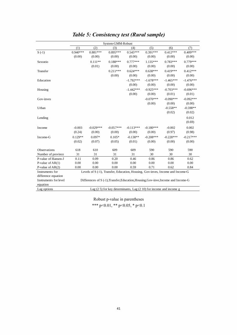
41

Table 5: Consistency test (Rural sample)

Robust p-value in parentheses

*** p<0.01, ** p<0.05, * p<0.1

System-GMM-Robust

(1) (2) (3) (4) (5) (6) (7)

S (-1) 0.940*** 0.881*** 0.895*** 0.545*** 0.391*** 0.412*** 0.409***

(0.00) (0.00) (0.00) (0.00) (0.00) (0.00) (0.00)

Sexratio 0.111** 0.188*** 0.777*** 1.135*** 0.783*** 0.779***

(0.01) (0.00) (0.00) (0.00) (0.00) (0.00)

Transfer 0.211*** 0.624*** 0.638*** 0.419*** 0.412***

(0.00) (0.00) (0.00) (0.00) (0.00)

Education -1.792*** -1.678*** -1.465*** -1.476***

(0.00) (0.00) (0.00) (0.00)

Housing -1.442*** -0.925*** -0.703*** -0.696***

(0.00) (0.00) (0.01) (0.01)

Gov-inves -0.070*** -0.090*** -0.092***

(0.00) (0.00) (0.00)

Urban -0.558** -0.598**

(0.02) (0.02)

Lending 0.012

(0.69)

Income -0.003 -0.029*** -0.057*** -0.113*** -0.180*** -0.002 0.002

(0.24) (0.00) (0.00) (0.00) (0.00) (0.97) (0.98)

Income-G 0.129** 0.097* 0.105* -0.138** -0.208*** -0.228*** -0.217***

(0.02) (0.07) (0.05) (0.01) (0.00) (0.00) (0.00)

Observations 618 610 609 609 590 590 590

Number of province 31 31 31 31 30 30 30

P-value of Hansen-J 0.11 0.09 0.20 0.46 0.86 0.86 0.62

P-value of AR(1) 0.00 0.00 0.00 0.00 0.00 0.00 0.00

P-value of AR(2) 0.00 0.00 0.00 0.59 0.71 0.62 0.84

Instruments for

difference equation

Levels of S (-1), Transfer, Education, Housing, Gov-inves, Income and Income-G

Instruments for level

equation

Differences of S (-1),Transfer,Education,Housing,Gov-inve,Income and Income-G

Lag options Lag (2 5) for key determinants, Lag (2 10) for income and income g

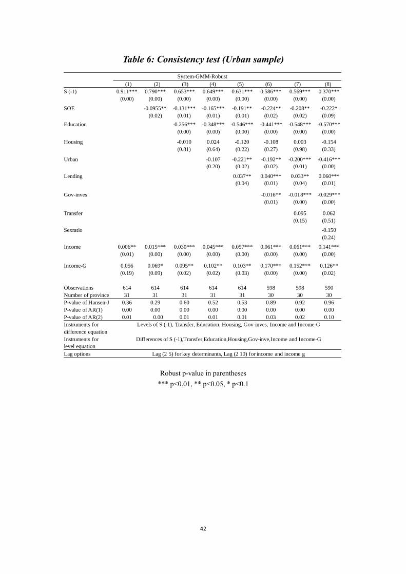
42

Table 6: Consistency test (Urban sample)

Robust p-value in parentheses

*** p<0.01, ** p<0.05, * p<0.1

System-GMM-Robust

(1) (2) (3) (4) (5) (6) (7) (8)

S (-1) 0.911*** 0.790*** 0.653*** 0.649*** 0.631*** 0.586*** 0.569*** 0.370***

(0.00) (0.00) (0.00) (0.00) (0.00) (0.00) (0.00) (0.00)

SOE -0.0955** -0.131*** -0.165*** -0.191** -0.224** -0.208** -0.222*

(0.02) (0.01) (0.01) (0.01) (0.02) (0.02) (0.09)

Education -0.256*** -0.348*** -0.546*** -0.441*** -0.548*** -0.570***

(0.00) (0.00) (0.00) (0.00) (0.00) (0.00)

Housing -0.010 0.024 -0.120 -0.108 0.003 -0.154

(0.81) (0.64) (0.22) (0.27) (0.98) (0.33)

Urban -0.107 -0.221** -0.192** -0.200*** -0.416***

(0.20) (0.02) (0.02) (0.01) (0.00)

Lending 0.037** 0.040*** 0.033** 0.060***

(0.04) (0.01) (0.04) (0.01)

Gov-inves -0.016** -0.018*** -0.029***

(0.01) (0.00) (0.00)

Transfer 0.095 0.062

(0.15) (0.51)

Sexratio -0.150

(0.24)

Income 0.006** 0.015*** 0.030*** 0.045*** 0.057*** 0.061*** 0.061*** 0.141***

(0.01) (0.00) (0.00) (0.00) (0.00) (0.00) (0.00) (0.00)

Income-G 0.056 0.069* 0.095** 0.102** 0.103** 0.170*** 0.152*** 0.126**

(0.19) (0.09) (0.02) (0.02) (0.03) (0.00) (0.00) (0.02)

Observations 614 614 614 614 614 598 598 590

Number of province 31 31 31 31 31 30 30 30

P-value of Hansen-J 0.36 0.29 0.60 0.52 0.53 0.89 0.92 0.96

P-value of AR(1) 0.00 0.00 0.00 0.00 0.00 0.00 0.00 0.00

P-value of AR(2) 0.01 0.00 0.01 0.01 0.01 0.03 0.02 0.10

Instruments for

difference equation

Levels of S (-1), Transfer, Education, Housing, Gov-inves, Income and Income-G

Instruments for

level equation

Differences of S (-1),Transfer,Education,Housing,Gov-inve,Income and Income-G

Lag options Lag (2 5) for key determinants, Lag (2 10) for income and income g

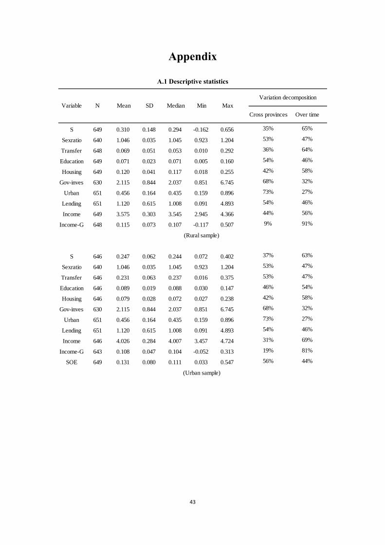
43

Appendix

A.1 Descriptive statistics

Cross provinces Over time

S 649 0.310 0.148 0.294 -0.162 0.656 35% 65%

Sexratio 640 1.046 0.035 1.045 0.923 1.204 53% 47%

Transfer 648 0.069 0.051 0.053 0.010 0.292 36% 64%

Education 649 0.071 0.023 0.071 0.005 0.160 54% 46%

Housing 649 0.120 0.041 0.117 0.018 0.255 42% 58%

Gov-inves 630 2.115 0.844 2.037 0.851 6.745 68% 32%

Urban 651 0.456 0.164 0.435 0.159 0.896 73% 27%

Lending 651 1.120 0.615 1.008 0.091 4.893 54% 46%

Income 649 3.575 0.303 3.545 2.945 4.366 44% 56%

Income-G 648 0.115 0.073 0.107 -0.117 0.507 9% 91%

(Rural sample)

S 646 0.247 0.062 0.244 0.072 0.402 37% 63%

Sexratio 640 1.046 0.035 1.045 0.923 1.204 53% 47%

Transfer 646 0.231 0.063 0.237 0.016 0.375 53% 47%

Education 646 0.089 0.019 0.088 0.030 0.147 46% 54%

Housing 646 0.079 0.028 0.072 0.027 0.238 42% 58%

Gov-inves 630 2.115 0.844 2.037 0.851 6.745 68% 32%

Urban 651 0.456 0.164 0.435 0.159 0.896 73% 27%

Lending 651 1.120 0.615 1.008 0.091 4.893 54% 46%

Income 646 4.026 0.284 4.007 3.457 4.724 31% 69%

Income-G 643 0.108 0.047 0.104 -0.052 0.313 19% 81%

SOE 649 0.131 0.080 0.111 0.033 0.547 56% 44%

(Urban sample)

Max

Variation decomposition

Variable N Mean SD Median Min

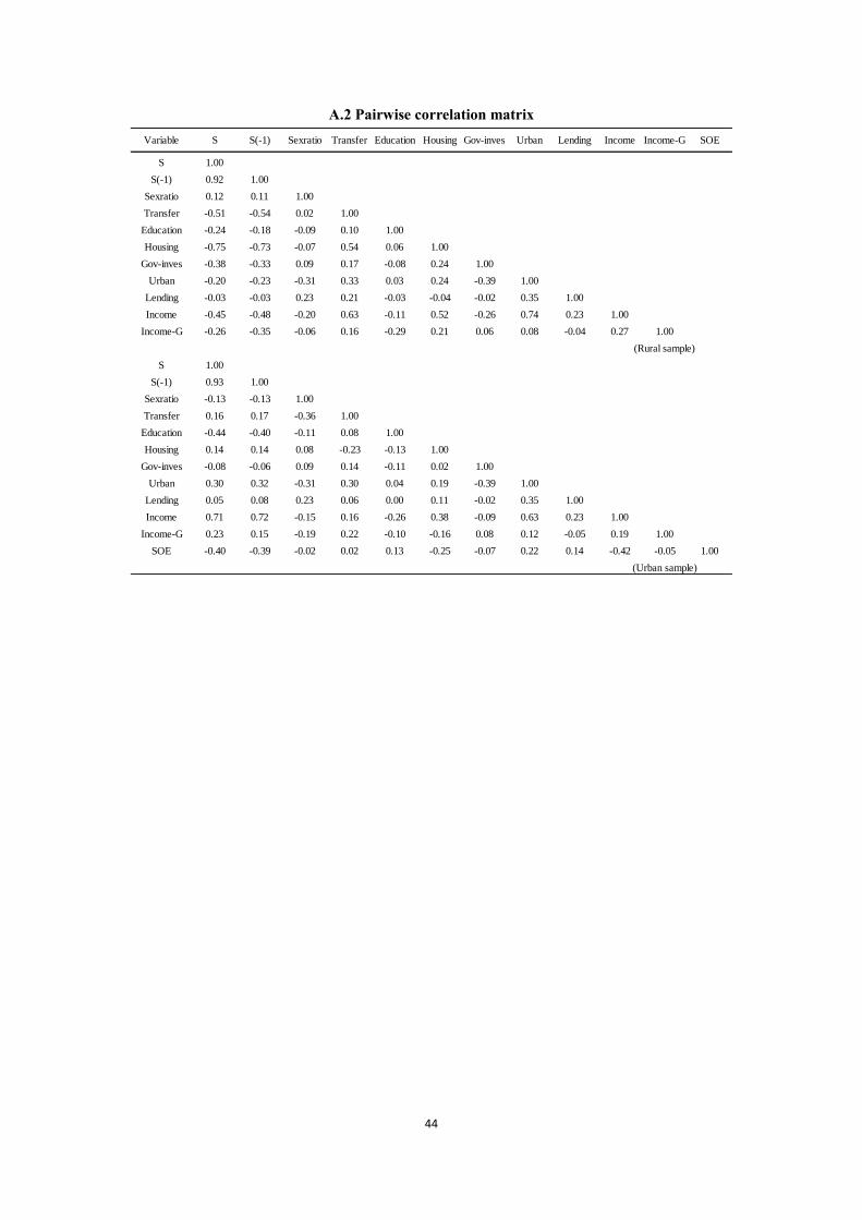
44

A.2 Pairwise correlation matrix

Variable S S(-1) Sexratio Transfer Education Housing Gov-inves Urban Lending Income Income-G SOE

S 1.00

S(-1) 0.92 1.00

Sexratio 0.12 0.11 1.00

Transfer -0.51 -0.54 0.02 1.00

Education -0.24 -0.18 -0.09 0.10 1.00

Housing -0.75 -0.73 -0.07 0.54 0.06 1.00

Gov-inves -0.38 -0.33 0.09 0.17 -0.08 0.24 1.00

Urban -0.20 -0.23 -0.31 0.33 0.03 0.24 -0.39 1.00

Lending -0.03 -0.03 0.23 0.21 -0.03 -0.04 -0.02 0.35 1.00

Income -0.45 -0.48 -0.20 0.63 -0.11 0.52 -0.26 0.74 0.23 1.00

Income-G -0.26 -0.35 -0.06 0.16 -0.29 0.21 0.06 0.08 -0.04 0.27 1.00

(Rural sample)

S 1.00

S(-1) 0.93 1.00

Sexratio -0.13 -0.13 1.00

Transfer 0.16 0.17 -0.36 1.00

Education -0.44 -0.40 -0.11 0.08 1.00

Housing 0.14 0.14 0.08 -0.23 -0.13 1.00

Gov-inves -0.08 -0.06 0.09 0.14 -0.11 0.02 1.00

Urban 0.30 0.32 -0.31 0.30 0.04 0.19 -0.39 1.00

Lending 0.05 0.08 0.23 0.06 0.00 0.11 -0.02 0.35 1.00

Income 0.71 0.72 -0.15 0.16 -0.26 0.38 -0.09 0.63 0.23 1.00

Income-G 0.23 0.15 -0.19 0.22 -0.10 -0.16 0.08 0.12 -0.05 0.19 1.00

SOE -0.40 -0.39 -0.02 0.02 0.13 -0.25 -0.07 0.22 0.14 -0.42 -0.05 1.00

(Urban sample)