Countercyclical Labor Income Risk and Portfolio Choices ...

Countercyclical Labor Income Risk and Portfolio Choices

over the Life-Cycle

Sylvain Catherine∗

September 12, 2018

Abstract

I structurally estimate a life-cycle model of portfolio choices that incorporates the rela-

tionship between stock market returns and the cross-sectional skewness of idiosyncratic labor

income shocks. The cyclicality of this skewness can explain (i) why young households with

modest financial wealth do not participate in the stock market and (ii) why, conditional on

participation, the share of financial wealth invested in equity slightly increases with age until

retirement. With an estimated relative risk aversion of 5 and yearly participation cost of

$290, the model matches the evolution of wealth, of stock market participation and of the

equity share of participants over the life-cycle. Without cyclical skewness, the same model

requires a risk aversion above 10 or a participation cost above $1,000 to match the average

equity share and cannot explain its decline over the life-cycle. Nonetheless, cyclical skewness

reduces the aggregate demand for equity by at most 15%.

Keywords: Household finance, Labor income risk, Portfolio choices, Human capital, Life-cycle

model, Simulated method of moments

JEL codes: G11, G12, D14, D91, J24, H06

∗The Wharton School, University of Pennsylvania.I am grateful to David Thesmar, Fatih Guvenen, Amir Yaron, Annette Vissing-Jørgensen, Jonathan Parker,

Hugues Langlois, Denis Gromb, Kim Peijnenburg as well as workshop participants at HEC Paris and the Universityof Minnesota. All errors are mine.

1 Introduction

Following Viceira (2001) and Cocco et al. (2005), a large literature studies how human capital risk

affects the optimal demand for stocks over the life-cycle. Because the correlation between stock

market returns and labor income shocks is close to zero, most papers conclude that human capital

is a substitute for bonds and should increase the demand for equity. This conclusion creates two

problems. First, as the share of human capital in total wealth declines over the life-cycle, so should

the share of financial wealth invested in equity (Jagannathan and R. Kocherlakota (1996)).1 This

prediction is not supported by the data. On the contrary, the stock market participation rate of

US households rises with age until retirement. Moreover, conditional on participation, the share

of financial wealth they invest in equity does not decrease before retirement (Bertaut and Starr-

McCluer (2002), Ameriks and Zeldes (2004)). Second, when human capital increases the demand

for stocks, life-cycle models need unrealistically high levels of risk aversion to match the average

equity share of working households.

These discrepancies are evidence that households make significant investment mistakes or that

economists do not understand the nature of their background risk. In particular, life-cycle models

ignore recent findings by Guvenen et al. (2014) that the cross-sectional skewness of labor income

shocks is cyclical. Cyclical skewness implies that the worst human capital shocks happen during

recessions, which themselves tend to coincide with financial crashes. As a consequence, workers

investing in the stock market take the risk of losing their job and a large fraction of their savings

at the same time. To illustrate this intuition, Figure 1 plots the evolution of the cross-sectional

skewness of earnings growth among the US male population and that of S&P500 returns between

1978 and 2010 and shows that these two series move together.

[Insert Figure 1 about here]

In this paper, I show that introducing cyclical skewness in a standard life-cycle model of

portfolio choices helps reconcile its predictions with the data and leads to more plausible estimates

of risk aversion. To do so, I follow the dominant approach in the literature by building a life-cycle

model in which a worker with constant relative risk aversion (CRRA) invests his wealth in a riskfree

1Beside these authors, Viceira (2001), Cocco et al. (2005), Campbell et al. (2001), Cocco (2005), Gomes andMichaelides (2005), Gomes et al. (2008), and Chai et al. (2011) reach the same conclusion.

1

asset or the stock market portfolio. The main innovation of the model is that it incorporates the

relationship between stock market returns and the cross-sectional skewness of idiosyncratic labor

income shocks. The model is estimated in two steps using the Simulated Method of Moments

(SMM). In the first step, I estimate the joint dynamics of labor income and stock market returns

using US Social Security panel data from 1978 and 2010. In a second step, I estimate the coefficient

of relative risk aversion, the discount factor and a yearly stock market participation cost. These

parameters are identified by the evolution of wealth, participation and equity holdings over the

life-cycle in the US Survey of Consumer Finances (SCF).

My main findings are as follows. First, my model matches the data well with a relative risk

aversion of γ = 5 and a yearly participation cost of only $290. Without cyclical model, the same

model requires a level of relative risk aversion above 10 or a participation cost above $1,000 to

match the average equity share and cannot explain its decline over the life-cycle. Second, compar-

ative statics show that cyclical skewness has a strong effect on households with modest financial

wealth. In particular, cyclical skewness causes the optimal equity share of young workers to prac-

tically drop from roughly 100% to close to 0%. Third, cyclical skewness has little consequences for

households with high financial-wealth-to-wage ratios. As a consequence, cyclical skewness reduces

the aggregate demand for equity by only 15% and increases the equity premium by at most half

a percentage point, which contradicts previous findings by Constantinides and Ghosh (2017).

The first step of my quantitative exercise is to estimate the dynamics of labor income and yearly

stock market returns. Idiosyncratic income shocks are modeled and estimated as in Guvenen et al.

(2014) with one key difference. Instead of taking two different values in recessions and expansions,

skewness is a continuous function of the average labor income shock, which itself correlates with

stock market returns. The labor income process is estimated by targeting the cross-sectional mean,

variance and skewness of idiosyncratic earnings growth in US Social Security data for each year

from 1978 to 2010. Importantly, each of these moments are targeted for earnings growth over 1,

3 and 5 year periods. This allows me to disentangle the dynamics of transitory and persistent

shocks and to estimate the persistence of the latter. In line with Guvenen et al. (2014), I find tail

shocks to be quite persistent, and therefore more likely to have important portfolio implications.

In a second step, I incorporate this labor income process into a standard life-cycle model of

portfolio choices. The model is similar to Cocco et al. (2005) but offers a more realistic computation

2

of Social Security pension benefits and takes into account the social safety net and stock market

crashes.

I start the structural estimation by assuming no participation cost. The agent’s discount

factor and relative risk aversion are identified by the evolutions of wealth and unconditional equity

shares over the life-cycle. The model with cyclical skewness closely matches these moments with

a discount factor of β = 0.95 and a relative risk aversion of γ = 7. By contrast, the model without

cyclical skewness cannot match the data and generates a very high estimate of γ (10.8) and a very

low estimate of β (0.79), in line with previous results by Fagereng et al. (2017).2

In a second set of estimations, I introduce a fixed yearly participation cost which I identify

using the evolution of stock market participation rates. For the model with cyclical skewness, I find

an estimated risk aversion of γ = 5.5 and a yearly participation cost of $290. This cost is enough

to prevent the participation of young workers with limited financial wealth because their optimal

equity share would be low in the absence of participation costs. By contrast, without cyclical

skewness, young households would have very high optimal equity shares. For this reason, matching

their low participation rate requires a much higher participation cost of $1,010. Though it can

match the evolution of participation rates, the model without cyclical skewness keeps generating

a negative relationship between age and the equity share of participants.

Using this set of parameter estimates, I run comparative statics to show that cyclical skewness

strongly reduces workers’ optimal equity share. For households with modest financial-to-human

wealth ratios, cyclical skewness reduces the optimal equity share from roughly 100% to close to

0%. Even absent any participation cost, most households with less than a year of salaries in wealth

barely hold any stocks. Moreover, for relative risk aversions as low as 5, cyclical skewness reverses

the predicted relationship between age and the equity share. I also find that, while the fear of

stock market crashes only reduces the equity share of young households by a few percentage points

when labor income shocks are normally distributed, its effect is much stronger in the presence of

cyclical skewness. Tail events on the stock market and in individuals’ careers matter more when

they tend to coincide.

To assess the model’s validity, I also evaluate its prediction regarding the relationship between

2Fagereng et al. (2017) estimate a similar model on Norwegian data and find γ = 11 and β = 0.77 with aparticipation cost of only $69.

3

the equity share and the wealth-to-wage ratio within age groups. I find this relationship to be

relatively flat in the data and in the model with cyclical skewness but to be strongly negative in

the model without cyclical skewness. Moreover, holding age and human capital fixed, the optimal

equity share in the presence of cyclical skewness is increasing and concave in financial wealth, a

pattern documented in Calvet and Sodini (2014)’s study of Swedish twins and which these authors

interpret as evidence of decreasing relative risk aversion.

Finally, I run counterfactual experiments to quantify the effect of cyclical skewness on the

aggregate demand for stocks and the equity premium. First, I start by removing cyclical skewness

from the model and shows that this increases the aggregate demand for equity by 9 to 15%. Then,

I solve for the change in the equity premium that exactly offsets this increase in demand and find

that a drop of 0.5 percentage points in the equity premium is enough to get the aggregate demand

for stocks back to its initial level. The modest magnitude of my results contrasts with findings by

Constantinides and Ghosh (2017) who argue that the cyclical skewness in consumption shocks can

explain the equity premium. These authors assume that all households face the same consumption

risk. I argue that this assumption is incorrect. Indeed, I show that if all households face the same

labor income risk, the negative skewness of consumption shocks during recessions is driven by

households with low financial wealth experiencing large negative labor income shocks. On the

other hand, workers with substantial financial wealth do not need to reduce their consumption

drastically when they receive the same labor income shocks. As a consequence, the cyclical

skewness of consumption risk documented by Constantinides and Ghosh (2017) is unlikely to

be representative of the risk faced by the average dollar-weighted investor.

Related literature My paper contributes to the literature on portfolio choices over the life-

cycle. We know from early studies that absent any background risk and labor income, the optimal

equity share of a CRRA investor does not vary with age (Merton (1969), Samuelson (1969)) and

that in the presence of risk-free human capital, households should move away from stocks as they

get closer to retirement (Merton (1971)). Even if human capital is risky, Viceira (2001) shows

that it increases the demand for equity as long as labor income risk is uncorrelated with stock

market returns. Cocco et al. (2005) document that the correlation between labor income shocks

and returns is close to zero and find that, in a calibrated life-cycle model, young households

4

with very high risk aversion invest all their wealth in stocks. Fagereng et al. (2017) structurally

estimate a similar model with stock market disasters using Norwegian data and find a relative

risk aversion between 11 and 15 and a discount factor between 0.75 and 0.83. Relative to these

papers, my contribution is to improve the model’s ability to match the data and generate more

realistic estimates of preference parameters, despite much more optimistic assumptions regarding

the distribution of stock market returns.3

To do so, my paper follows the intuition of Storesletten et al. (2007) and Lynch and Tan (2011)

that labor income risk is countercyclical. Relying on findings by Storesletten et al. (2004), these

authors assume that the variance of labor income shocks is higher during recessions and show that

this can generate a positive relationship between the optimal equity share and age. However, an

important issue with these papers is that US administrative data show no evidence that variance is

countercyclical (Guvenen et al. (2014)). Another closely related study is Benzoni et al. (2007) who

document that aggregate wages and dividends are cointegrated and show that this cointegration

may also generate a positive relationship between age and the optimal equity share when the

volatility of dividend growth is set to match that of stock market returns. However, de Jong

(2012) shows that this finding is not robust when stock returns are affected by other factors than

dividend growth, such as time-varying discount rates. Overall, my paper confirms that labor

income risk can generate a positive relationship between age and the optimal equity share, but,

by contrast to previous studies, relies on well documented assumptions.

My paper also re-examines Mankiw (1986)’s idea that the concentration of aggregate shocks

among a few individuals matters for asset pricing. Storesletten et al. (2007) and Constantinides

and Ghosh (2017) respectively study the effects of countercyclical variance in labor income risk and

cyclical skewness in consumption risk. My contribution to this literature is to show that, unless

wealthy households face greater countercyclical labor income risk, the latter can only explain a

limited fraction of the equity premium.

My paper also contributes to the literature on stock market participation. Vissing-Jorgensen

(2002) argues that a yearly participation cost of $260 can explain the decision of 75% of non

3The equity premiums in Fagereng et al. (2017) and my paper are respectively 0.03 and 0.05, while the standarddeviations of returns are 0.24 and 0.16. These numbers imply that, in Merton’s model, I would need a relative riskaversion 2.5 times larger to match the same equity share.

5

participants. However, Andersen and Nielsen (2011) and Briggs et al. (2015) show that windfall

wealth has limited effects on participation, which is not consistent with limited participation being

caused by fixed costs. In my model, matching the rise of participation over the life-cycle requires a

much higher cost when cyclical skewness is ignored. When it is taken into account, estimated costs

are relatively low and cannot fully explain participation levels, leaving more space for alternative

theories, which is more consistent with Andersen and Nielsen (2011) and Briggs et al. (2015).

2 Model

This section describes a discrete time life-cycle model of consumption and portfolio choices. The

main novelty of this model is that the distribution of idiosyncratic labor income shocks tends to

have negative (positive) skewness in years of bad (good) stock market returns.

2.1 Macroeconomic environment

Stock market returns The log return of the stock market index on year t is

st = s1,t + s2,t (1)

where s1 denotes the component of stock returns that covaries with labor market conditions. To

take into account stock market crashes, I assume that s1 follows a normal mixture distribution:

s1,t =

s−1,t ∼ N (µ−s , σ2s1

) with probability ps

s+1,t ∼ N (µ+s , σ

2s1

) with probability 1− ps(2)

whereas s2,t is normally distributed with variance σ2s2

. Without loss of generality, I impose µ−s < µ+s

and interpret µ−s as the expected log return in years of stock market crashes, and ps the frequency

of such events. On the other hand, µ+s is the expected log return during normal years.

6

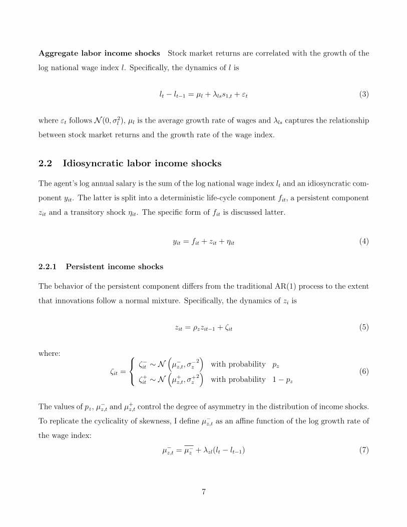
Aggregate labor income shocks Stock market returns are correlated with the growth of the

log national wage index l. Specifically, the dynamics of l is

lt − lt−1 = µl + λlss1,t + εt (3)

where εt follows N (0, σ2l ), µl is the average growth rate of wages and λls captures the relationship

between stock market returns and the growth rate of the wage index.

2.2 Idiosyncratic labor income shocks

The agent’s log annual salary is the sum of the log national wage index lt and an idiosyncratic com-

ponent yit. The latter is split into a deterministic life-cycle component fit, a persistent component

zit and a transitory shock ηit. The specific form of fit is discussed latter.

yit = fit + zit + ηit (4)

2.2.1 Persistent income shocks

The behavior of the persistent component differs from the traditional AR(1) process to the extent

that innovations follow a normal mixture. Specifically, the dynamics of zi is

zit = ρzzit−1 + ζit (5)

where:

ζit =

ζ−it ∼ N(µ−z,t, σ

−z2)

with probability pz

ζ+it ∼ N(µ+z,t, σ

+z2)

with probability 1− pz(6)

The values of pz, µ−z,t and µ+

z,t control the degree of asymmetry in the distribution of income shocks.

To replicate the cyclicality of skewness, I define µ−z,t as an affine function of the log growth rate of

the wage index:

µ−z,t = µ−z + λzl(lt − lt−1) (7)

7

Since idiosyncratic shocks have an expectation of zero, I impose

pzµ−z,t + (1− pz)µ+

z,t = 0 (8)

and, without loss of generality, pz ≤ 0.5. In this case, and if σ−z is large, pz can be interpreted

as the frequency of tail events, which tend to be promotions during expansions and layoffs in

recessions.

2.2.2 Transitory income shocks

The transitory component of income is also modeled as a mixture of normals whose first and

second components always coincide with the first and second components of the normal mixture

governing the innovations to zi.

ηit =

η−it ∼ N (0, σ−η2) if ζit = ζ−it

η+it ∼ N (0, σ+η2) if ζit = ζ+it

(9)

2.3 Pensions and safety net

2.3.1 Social Security

In the US, wages are subject to a Social Security payroll tax of τ = 12.4% up to a limit known

as the maximum taxable earnings and close to 2.5 times the national wage index4. Pensioners

receive a percentage of the value of the national wage index when they retired. This percentage

depends on the agent’s historical taxable earnings, adjusted for the growth in the national wage

index. Specifically, the initial pension Pi of agent i is defined by:

4In 2014, the value of the Social Security wage index was $46, 481 and the maximum amount of taxable earningswas $117, 000

8

PiLR

=

0.9× SiR if SiR < 0.2

0.116 + 0.32× SiR if 0.2 ≤ SiR < 1

0.286 + 0.15× SiR if 1 ≤ SiR.

(10)

where LR = elR is the value of the wage in the first retirement year and SiR is the agent’s average

historical taxable earnings. Specifically,

Sit =t∑

k=t0

max Yik, 2.5t− t0 + 1

(11)

where Yik = eyik . Because Social Security uses a bend point system, returns on investment are

higher for individuals with low earnings records.

To avoid keeping track of historical earnings, many papers in the life-cycle literature model

Social Security benefits as a percentage of the agent’s last persistent/permanent income, a method-

ology that overestimates Social Security risk. In my model, a large negative shock close to retire-

ment would have dramatic consequences on the value of Social Security entitlements, which is not

the case in reality. To solve this problem, I keep track of the agent’s average historical earnings.

2.3.2 Social safety net

Welfare programs limit the impact of human capital disasters on consumption, and thus may also

alleviate the portfolio consequences of cyclical skewness. To take this into account, I incorporate

into the model the Supplemental Nutrition Assistance Program (also known as the food stamp

program) and, for individuals above 65 years, the Supplemental Security Income (SSI) program.

Eligibility to these programs is limited to individuals with very low financial wealth (roughly

$2,000), which I model as less than 5% of the average national wage. After 65 years old, eligible

individuals receive supplemental income such that their total income reaches at least 20% of the

national average wage. Before 65 years old, eligible individuals with earnings below 20% of the

national average wage receive benefits equal to that threshold minus 30% of their earnings. Hence,

welfare benefits are defined by:

9

Bit

Lit=

max

0.2− PiLit, 0

if Wit

Lit< 0.05 and t ≥ R

max 0.2− 0.3Yi, 0 if Wit

Lit< 0.05, Yi < 0.2 and t < R

(12)

2.4 Household

I incorporate the stochastic model in the life-cycle problem of an agent controlling his consumption

C and equity share π.

Preferences The agent has CRRA preferences and maximizes his expected utility, given by

Vt0 = ET∑t=t0

βt−1

(t−1∏k=0

(1−mk)

)C1−γit

1− γ(13)

where γ is his coefficient of relative risk aversion, mk the mortality rate at age k, β the discount

factor and T the maximum lifespan.

Wealth dynamics Each year, he receives an income Iit that includes his net wage, pension and

welfare benefits, that is:

Iit = (Yit − τ max Yit, 2.5)Lt +Bit + Pit (14)

He decides how much to consume, and then invests his savings in bonds or in the stock market

index. Short-selling and borrowing are not allowed. Holding equity incurs a fixed participation cost

cπ,1 and a variable management fee cπ,2. I assume that cπ,1 and cπ,2 are respectively percentages

of the wage index and assets under management. Noting π the equity share and r the risk free

rate, the agent’s wealth dynamics is

Wit+1 = [Wit + Iit − Cit][πite

st−cπ,2 + (1− πit)er]− 1πit>0cπ,1Lt (15)

Dynamic optimization The problem is solved by dynamic programming. Besides age, the

state variables of the problem are the components of labor income l, zi and ηi, Social Security

record Si and financial wealth Wi. Dropping indexes to simplify the notation, the Bellman equation

10

is

Vt(w, l, z, η, S) = max[Ct,π]

C1−γt

1− γ+ (1−mt) βEVt+1

(16)

and the terminal value is the period utility derived from entirely consuming pension, benefits and

financial wealth.

VT (w, l, S) =(W + P +B)1−γ

1− γ(17)

Homothety of the value function Since the agent has CRRA, and because all benefits and

participation costs are proportional to Lt, the dimensionality of the problem can be reduced by

scaling financial wealth, wages and pension benefits by the national wage index. Noting x = w− l

the log of the financial wealth to wage index ratio, we have

Vt(w, l, z, η, S) = e(1−γ)lVt(x, 0, z, η, S). (18)

3 Estimation

The model is estimated in two steps. In the first step, I use moments derived from Social Security

panel data and S&P500 data to estimate the parameters controlling the dynamics of wages and

stock market returns. In a second step, I use data on the portfolio of US households to estimate

their preferences and a fixed yearly stock market participation cost.

3.1 Data

The estimation uses two US datasets: the Social Security Master Earnings File (MEF) and the

Survey of Consumer Finances (SCF).

Labor income risk Lacking access to the MEF, I rely on Guvenen et al. (2014) who report

cross-sectional moments (mean, standard deviation, skewness) of the distribution of log labor

income growth, net of life-cycle effects, for a representative sample of the US male population

11

between 25 and 60 years old, for each year from 1978 to 2010. I also rely on Guvenen et al. (2015)

who report the evolution of within-cohort wage inequalities for the same sample.

Households’ portfolios Moments relative to the wealth and portfolio choices of households are

computed using the triennial Survey of Consumer Finances (SCF). I use publicly available data

from nine waves between 1989 and 2013. I use survey weights, adjusted to give equal importance

to all surveys. I restrict my sample to households between 23 and 82 years old, who are not

business owners (bus=0) and whose net worth (networth) exceeds -$10,000. Table 4 reports key

statistics for the final sample. Households constitute the unit of analysis.

[Insert Table 4 about here]

I define wealth as net worth normalized by the national average wage. The average wage in

each survey is computed by taking the mean of wage incomes (wageinc) for households whose head

is between 22 and 65 and part of the labor force (lf =1). The equity share is defined as equity

holdings (equity) divided by financial wealth (fin), for households with positive financial wealth.

3.2 Stock market returns and labor income risk

The first step of the structural estimation is dedicated to the stochastic processes controlling

macroeconomic and idiosyncratic shocks, which are estimated independently.

3.2.1 Macroeconomic shocks

Eight parameters control the dynamics of stock returns and aggregate labor income shocks: ps,

µ−s , µ+s , σs1 , σs2 , µl, λls, σl. I estimate these parameters by SMM by targeting moments from

the time series of the average wage growth and yearly S&P500 returns. The first 8 moments are

the mean, standard deviation, and the third (skew) and fourth (kurtosis) standardized moments

of each time-series. The last moment is the correlation coefficient of the two time series. Stock

market moments are computed using yearly data between 1900 and 2015. The time series of

average wage growth goes from 1978 to 2010.


12

Table 1 reports the results of the estimation and shows that, despite being slightly overiden-

tified, the model matches all moments very well. Note that the model is conservative regarding

the frequency and severity of financial crashes. In the model, log returns below −.35 (≈ −30%)

occur three times per century. In the data, this actually happened five times since 1900 (1917,

1931, 1937, 1974 and 2008). For a log return of −.35, workers should expect their wage to drop by

approximately 5%.5 For the 2008 crisis, the model predicts an expected log wage shock of −.062

versus −.064 in the data.

3.2.2 Idiosyncratic shocks

Eight parameters control the distribution of idiosyncratic labor income shocks: pz, ρz, µ−z , λzl, σ−z ,

σ+z , σ−η , σ+

η . To estimate these parameters, I simulate an economy receiving the same aggregate

shocks as the US economy between 1944 and 2010.6 For each year between 1978 and 2010, I target

the historical values of Kelly’s skewness at the one, three and five-year horizons, as well as the

standard deviation at the one and five-year horizons.7 This constitutes a first set of 155 empirical

moments targeted in the SMM.

The cyclicality of skewness is identified by targeting the historical values of these moments

for each of the 33 years and using the true time series of aggregate labor income shocks as an

input. The decomposition of the variance between transitory (σ−η , σ+η ) and persistent shocks (σ−z ,

σ+z ) and the persistence of the latter (ρz) are identified by targeting these moments at different

horizons. One concern is that the model could overestimate the persistence of labor income shocks

if workers face different life-cycle income profiles ex-ante (Guvenen (2009)). To address this issue,

I assume that the deterministic component of yi is of the form

fi(t) = f(t) + ϕit+ αi (19)

where f(t) is a function of experience common to all workers while the two other terms are

individual specific and normally distributed with standard deviations σα and σϕ. Note that the

50.008− 0.161 ∗ 0.35 = 0.0486I use the NIPA tables to estimate aggregate income shocks before 1978.7Guvenen et al. (2014) do not report the standard deviation at the three-year horizon.

13

main role of these parameters is to get a conservative estimate of ρz.8 To avoid the multiplication

of state variables, I ignore σϕ in the life-cycle model and uses σα to initialize the distribution of

zi.

To identify σα and σϕ, I also target the evolution of within-cohort inequalities between 25

and 60 years. Hence, I use 191 moments to estimate 10 parameters. To maintain a constant age

structure within the economy, I start the simulation in 1944 and replace each cohort reaching 60

with young workers. More details on the estimation procedure are provided in Appendix A.1.

Table 2 reports the results of the SMM and Figure 2 plots targeted and simulated moments.

The model replicates correctly the cyclicality of skewness at different horizons as well as the

stability of the standard deviation and, unlike Guvenen et al. (2014), its high value.9



A standard deviation of labor income shock above 0.5 may seem counter-intuitive but can be

explained by the high peakness of the distribution. Since pz = .136, in any given year, 86.4% of

workers receive shocks from normal distributions with relatively low standard deviations: respec-

tively 0.037 and 0.089 for the persistent and transitory components. This means that most of

the variance comes from the remaining 13.6% who receive shocks with very high standard devia-

tions: respectively 0.562 and 0.895. A plausible economic interpretation is that a fraction of the

population switches job or become unemployed while the vast majority does not experience any

noticeable shock.

Another important result is the very high persistence of innovations to z. By increasing the

volatility of the human capital stock, an overestimation of ρz would create spurious portfolio

effects, in particular among young households. Four things can reduce this concern. First, my

8The literature on labor income risk offers two alternative views on the rise of within-cohort inequalities overthe life-cycle. In models with “restricted income profiles” (RIP), workers face similar life-cycle income profilesand inequalities result from large and highly persistent shocks. By contrast, models with “heterogeneous incomeprofiles” (HIP) assume individual specific deterministic drifts and require lower shock persistence to explain thedata (see Guvenen (2009)). I adopt the HIP specification, which is the less likely to overstate the role of incomerisk in portfolio choices by overestimating ρz.

9In Guvenen et al. (2014), transitory shocks are normally distributed and the model cannot match the standarddeviation. I find that this problem can be solved by modeling transitory shocks using the normal mixture describedin equation (9)

14

estimate of ρz is below that of the baseline specification of Guvenen et al. (2014). Second, the

model matches the ratio of standard deviations at the five and one year horizons, a simple measure

of persistence. Third, the model does not exaggerate the evolution of within-cohort inequalities

over the life-cycle. Finally, the high persistence must be interpreted in conjunction with the high

value of σ−η , which indicates that a large fraction of the most extreme shocks is transitory and

recovered within one year. Therefore, only shocks that do not quickly dissipate turn out to be very

persistent. This is consistent with findings by Guvenen et al. (2015) that workers who experience

a large drop in their income recover one-third of that loss within one year, but have to wait 10

years to recover more than two-thirds.

3.3 Preferences and participation cost

In the second step of the structural estimation, I use SCF data to estimate the coefficient of

relative risk aversion, the discount factor and a fixed yearly participation cost. Technical details

on the numerical resolution of the model and its estimation are provided in Appendix B.

3.3.1 Preset parameters

Table 3 reports preset parameters. I set the real interest rate to 2% and variable management fees

to 1%. From the agent’s point of view, this calibration implies an equity premium slightly above

5%, in the upper range of values used in previous papers.


I approximate f(t) with a quadratic polynomial that matches the average log wage by age ob-

served in Social Security data. Households start working at 23 and retire at 65. Death probabilities

are taken from Social Security actuarial life tables.

In the data, households start with different levels of wealth. I compute the centiles of the

distribution of wealth between 23 and 24 years old in the SCF and use them to generate 100

groups with different initial wealth in my simulation. Having all households start with the same

level of wealth would lead to an initial participation rate close to one or zero.

15

3.3.2 Identification

I run several sets of estimations and target the evolution over the life-cycle of the following vari-

ables: financial wealth, conditional or unconditional equity share, and stock market participation

rate.

Empirically, the relationship between these variables and age is estimated as follows. First, I

build 3-years age and cohort groups as in Ameriks and Zeldes (2004). Since the SCF is triennial,

each cohort group moves exactly from one age group to the next between two surveys. Second, I

disentangle age effects from year and cohort effects using the methodology of Deaton and Paxson

(1994), as in Fagereng et al. (2017). Specifically, for each variable of interest, I run OLS regressions

on a set of age, year and cohort group dummies and solve the collinearity problem by assuming

that year dummies sum to zero and are orthogonal to a time trend. As a result, any time trend is

captured by cohort effects. Finally, I compute the predicted values of each variable, for each age

group between [23; 25] and [62; 64], putting equal weights on all cohorts born after 1946.

This constitutes a vector m of 3× 14 = 56 empirical moments. The SMM procedure seeks the

parameters γ, ϕ and cπ,1 that minimize

(m− m (γ, ϕ, cπ,1))′W (m− m (γ, ϕ, cπ,1)) (20)

where m (γ, ϕ, cπ,1) is the vector of simulated moments generated by the model, and W is the

inverse of the covariance matrix of the empirical moments, which is estimated by bootstrapping

the true data. As described in the following section, some moments are not targeted across all

specifications.

The identification is straightforward and well understood. A higher discount factor (β) reduces

the accumulation of financial wealth. A higher risk aversion (γ) reduces the optimal equity share.

Finally, a higher fixed participation cost prevents the participation of households whose optimal

equity share represents a small dollar amount.

3.3.3 Results

Models without participation cost I start by estimating the coefficient of relative risk aver-

sion and the discount factor by targeting the evolutions of wealth and that of the unconditional

16

equity share. Estimation results for the models with and without cyclical skewness are respectively

reported in columns (1) and (4) of Table 5. Simulated moments and their empirical counterparts

are reported in Panel A of Figure 3.

Without cyclical skewness, the SMM fails to match the data and returns unlikely estimates of

the discount factor (β = 0.79) and relative risk aversion (γ = 10.81). The bond-like properties

of human capital imply a positive relationship between the human-to-financial wealth ratio and

the optimal risky share, and therefore a decline of the equity share over the life-cycle. A low β

mitigates this problem by slowing down the decline of the human-to-financial wealth ratio, but

this prevents the model from matching the level of wealth at 65. My estimates are very close

to Fagereng et al. (2017), who find γ = 11 and β = 0.77 in a similar model with stock market

disasters and a small participation cost of $69.

When cyclical skewness is taken into account, human capital is no longer bond-like and the

model is able to match the data with more reasonable estimates of the discount factor (β = 0.95)

and relative risk aversion (γ = 6.97).

Models with participation cost In a second step, I introduce a fixed yearly participation cost

and estimate it, alongside β and γ. To do so, I distinguish the intensive and extensive margins

by targeting the evolution of stock market participation rates and that of the equity share among

participants. Columns (2) and (5) of Table 5 reports the results and Panel B of Figure 3 the model

fitness.

Without cyclical skewness, participation costs improve the model’s ability to fit the data and to

produce more plausible estimates of β and γ. Estimated participation costs represent 2.1% of the

average wage, that is $1,010 in 2015. When human capital is bond-like, matching low participation

rates among young workers requires high fixed-costs because workers with low financial wealth

want to invest their entire wealth in the stock market. By preventing their participation, the fixed

cost also reduces the average conditional equity share, which, in turn, affects the estimated value

of γ, which falls from 10.79 to 6.46. The discount factor rises from 0.79 to 0.95 because wealth

accumulation drives the rise in participation. However, the model still fails to match the positive

relationship between age and the conditional equity share.

With cyclical skewness, estimated participation costs are much lower, representing only 0.6% of

17

the average wage ($290). Because workers with low financial wealth would not want to invest much

in the stock market anyway, a lower fixed cost is required to match low participation rates among

young households. The model still generates a conditional equity share that slightly increases with

age but overestimates participation among older households.

4 Discussion

4.1 Policy function

Portfolio choice models generally predict that human capital increases (decreases) the demand

for stocks when its exposure to stock market risk exceeds (is below) the agent’s optimal risky

share. This generally implies that, absent participation costs, the optimal equity share should be

a monotonous function of the wage-to-financial wealth ratio. This intuition does not hold in the

presence of cyclical skewness. This is apparent in Panel A of Figure 4, which plots the optimal

equity share of a 40 years old agent as a function of his persistent income (z) and financial wealth

(w). Panel B displays the same policy function assuming that labor income shocks are normally

distributed.


In Panel A, for a given level of human capital (z), the optimal equity share first increases with

financial wealth, reaches a maximum, and then decreases. By contrast, financial wealth always

reduces the optimal equity share in Panel B. In this case, human capital unambiguously generates

a positive demand for stocks as in Viceira (2001), because the covariance between labor income

shocks and stock market returns is negligible.

The difference between the two surfaces represents the effect of cyclical skewness, which is the

strongest for households with high wage-to-financial wealth ratios (z−w). From the agent’s point

of view, what matters is the risk of severe shocks to her lifetime consumption. His fear of losing

his job during a recession is therefore much more serious when most of his future consumption

depends on labor income. A simple way to hedge against this risk would be to short-sell the stock

market.

18

As the agent starts accumulating financial wealth, disastrous labor income shocks have milder

implications in terms of consumption. Because left-tail consumption risk becomes less of a concern,

the agent gives more attention to the low covariance between labor income shock and stock returns

and the optimal equity becomes a positive function of z and negative function of w. At the limit,

when w − z gets very large, the agent follows portfolio rules close to Merton’s solution.10

4.2 Empirical policy function

To evaluate my two models, I now turn to their ability to replicate empirical policy functions,

that is relationships between the current state of the household and its portfolio choice. Empirical

policy functions offer a natural starting point for model evaluation (Bazdresch et al. (2018)).

Beside age, the main state variable of the model that we observe in the data is the wage-

to-wealth ratio. Hence, I start by estimating the empirical relationship between the conditional

equity share and twenty quantiles of wage-to-wealth ratio using OLS with age and cohort fixed-

effects. Then, I run the same OLS regression in simulated data from my models with and without

cyclical skewness using estimated parameters reported in columns (2) and (5) of Table 5. The

OLS coefficients for all quantile dummies are reported in Figure 5.


Clearly, the model with cyclical skewness fits the empirical policy function much better. In

the SCF data, the conditional equity share and the wage-to-wealth ratios are not correlated. This

is also true in simulated data from the model with cyclical skewness. On the contrary, simulated

data from the model without cyclical skewness show a strong positive relationship between the

wage-to-wealth ratio and the conditional equity share. Given the low correlation between labor

income shocks and stock market returns, this relationship is consistent with theoretical predictions

from Viceira (2001). Hence, only the model with cyclical skewness matches how the equity share

of stock market participants varies within age-groups.

Note that the relationship between age and the equity share used to estimate the model is also

an empirical policy function. But this relationship is mostly driven by the evolution of the human

10Assuming normally distributed log-returns, the solution to Merton’s portfolio problem is µ−rγσ2 = .063−.02

5.6×.1892 ≈ .21

19

capital-to-financial wealth ratio. Indeed, without labor income, the optimal equity share would

be independent of age and wealth (Samuelson (1969), Merton (1969)). One can therefore argue

that the relationship between the equity share and the wage-to-wealth ratio provides a more direct

benchmark to evaluate the model.

We also know from Calvet and Sodini (2014)’s study of Swedish twins that (i), controlling for

human capital, the elasticity of the risky share to financial wealth is positive, and (ii) that this

elasticity is three times larger in the bottom quartile of financial wealth than in the top quartile.

Figure 4 shows that these two facts can only be reconcile with the model when it incorporates

cyclical skewness.

4.3 Decomposition of effects

In this section, I show that cyclical skewness has a strong effect on the optimal equity share and

that, without cyclical skewness, stock market disasters would not matter nearly as much. I also

find that taking into account Social Security is important to match the data.

To do so, I start by simulating the model with normally distributed income shocks and returns,

using parameter estimates reported in column (2) of Table 5. Then, I introduce or remove specific

elements of the model to see how the simulated data change. Figure 6 reports the evolution of the

equity share over the life-cycle depending on the presence of cyclical skewness and stock market

disasters.


Normally distributed shocks Scenario (a) represents the evolution of the equity share when

all shocks are normally distributed and shocks to human capital are only correlated with stock

returns at the national level. This calibration of the model is similar to the situation considered by

Cocco et al. (2005) and Viceira (2001), but with a lower level of risk aversion and higher variance

of labor income shocks. In the absence of participation costs, the result is quantitatively close to

Cocco et al. (2005).

Stock market disasters Scenario (b) takes into account stock market crashes. In my model,

taking into account the left-tail risk of the stock market reduces the optimal equity share by only

20

a few percentage points. In Fagereng et al. (2017), the introduction of left-tail risk in stock returns

has an effect three times larger on the optimal equity share, but the difference may arise from the

much higher levels of risk aversion (γ ≥ 10) considered by these authors.

Cyclical skewness In Scenario (c), households face cyclical skewness, but stock returns are log-

normally distributed. Introducing cyclical skewness has a dramatic effect on the level of the equity

share and reverses the sign of its relationship with age. For young households, absent participation

costs, the optimal equity share drops from close to 100% to close to 0%. The effect is much smaller

for households getting closer to retirement because most of their future consumption comes from

financial wealth ans Social Security entitlements.

Cyclical skewness & Stock market disasters Scenario (d) combines the effects of scenarios

(b) and (c). The difference between (c) and (d) is greater than between (a) and (b) which suggests

an interaction effect between cyclical skewness and stock market crashes. For young agents with

high wage-to-financial wealth ratios, cyclical skewness strongly amplifies the importance of stock

market tail risk. When income shocks are normally distributed, stock market tail risk reduces

the optimal equity share by roughly 6 percentage points over the entire life-cycle. By contrast,

assuming no participation cost, when cyclical skewness is taken into account, stock market tail

risk reduces π by 16 percentage points at 25 years old, 11 points at 35, 8 points at 45 and 6 points

at 55.

Social Security To a large extent, Social Security acts as a mandatory investment in bonds. If

entitlements perfect bond properties, and under the assumptions that (i) the mandatory yearly

investment is below the optimal saving rate of the agent, (ii) that the total investment in Social

Security entitlements is less than what the agent wants to invest in bonds, then one dollar of

investment in Social Security should reduce financial wealth and bond holdings by one dollar, but

equity holdings should be unaffected.


Panels A and B of Figure 7 appear to be in line with these predictions at retirement age.

However, equity holdings are slightly reduced by Social Security among younger households, which

21

is consistent with the facts that entitlements are somewhat risky as their value evolves with the

national wage index. The evolution of the equity share, reported in Panel C, is quite different

with Social Security. In the second half of the agent’s career, the risky share is higher because

entitlements reduce financial wealth, and therefore the denominator. In the first half of the

agent’s career, the risky share is lower. One possible explanation is that payroll taxes delay

the accumulation of precautionary savings. Unlike financial wealth, Social Security entitlements

cannot be used to smooth consumption in the event of a large negative income shock. This lack

of liquidity could deter workers from investing in stocks.

At age 65, equity holdings are identical in the two scenarios. At that point, Social Security

entitlements are risk-free and crowd out bonds. We know from Merton (1971) that optimal equity

holdings represent the same fraction of total wealth, including the present value of entitlements.

Hence, identical equity holdings in the two scenarios indicate identical total wealth and perfect

substitution between Social Security and private savings.

Social safety net I also run a counterfactual experiment in which I remove the SNAP and SSI

welfare programs. I find that the effect of these programs on the equity share does not exceed

a few percentage points, and only at the beginning of the life cycle. In the model, households

quickly accumulate enough wealth to become ineligible to these programs, which, of course, is not

true empirically.

4.4 Aggregate effect on the demand for equity

How does the cyclical skewness of labor income risk affect the optimal demand for equity and

the equity premium? To answer this question, I run a counterfactual experiment in which I

assume that labor income shocks are normally distributed, but have otherwise the same variance,

persistence and covariance with stock market returns. Holding the equity premium constant, I

then compute the change in the aggregate demand for equity in simulated data, including from

retired households. This change represents the effect of cyclical skewness on the demand for

equity. In a second step, I solve for the change in the equity premium that offsets the effect of

cyclical skewness and raises the aggregate demand for stocks back to its initial value. This change

22

corresponds to the effect of cyclical skewness on the equity premium assuming that the supply of

stocks in inelastic, and therefore represents an upper bound on the effect of cyclical skewness.

As reported in columns (1) and (2) of Table 6, I find that cyclical skewness reduces aggregate

demand for stocks by only 13% to 15%, a reduction that could be offset by increasing the equity

premium by half a percentage point. Columns (1) and (2) corresponds to the specifications with

and without fixed participation costs. The effect of cyclical skewness on the demand for equity

can be decomposed into two components. First, cyclical skewness reduces the share of aggregate

financial wealth invested in equity by 17% to 21%. But cyclical skewness also increases aggregate

financial wealth by 4% to 5% by stimulating precautionary savings, which attenuates the first

effect.


These findings contrast with the conclusions of Constantinides and Ghosh (2017), who argue

that cyclical skewness in consumption risk can explain a variety of asset pricing puzzles, including

the equity premium. One key difference between their methodology and mine, is that Constan-

tinides and Ghosh (2017) assume all households to face the same distribution of consumption

shocks and estimate their model by targeting the cross-sectional skewness of consumption growth.

By contrast, I assume all households to face the same distribution of labor income shocks. Under

my assumption, the distribution of consumptions shocks is very different across the wealth dis-

tribution. Households with very high wage-to-wealth ratios reduce their consumption drastically

when they receive a dramatic labor income shocks, but households with high financial wealth do

not. Hence, the negative skewness in the cross-sectional distribution of household consumption

growth documented by Constantinides and Ghosh (2017) is probably not representative of the risk

faced by the average dollar-weighted investor.

To further illustrate this intuition, Figure 8 plots the contribution of different deciles of financial

wealth and age to the cyclical skewness of consumption risk in simulated as well as their share of

aggregate financial wealth. Here, I measure cyclical skewness using cokurtosis, defined as:

κ =E[(δc − E(δc))

3 (s− E(s))]]

σ3δcσs

(21)

23

where δc,it = log(Cit+1

Cit

)is the growth rate of consumption of household i and σδc its cross-sectional

standard deviation. A large κ indicates that the distribution of δc is left (right) skewed in years

of low (high) stock returns. Because κ is a sum over households, computing the contribution

of each subgroup to κ is straightforward. As shown in Figure 8, individuals with low financial

wealth contribute disproportionately to κ. By contrast, the top decile concentrates close to 50%

of financial wealth and barely contributes to κ. Hence, the countercyclical consumption risk faced

by the average household cannot explain the behavior of the average dollar-weighted investor.


5 Robustness

5.1 Alternative theories of stock market participation

My estimation relies on the assumption that a fixed monetary cost explains low stock market par-

ticipation rates. This assumption is difficult to reconcile with reduced-form evidence that windfall

wealth has limited effects on participation (Andersen and Nielsen (2011), Briggs et al. (2015)).11

Moreover, a number of alternative solutions to the participation puzzle has been proposed: lack of

trust (Guiso et al. (2008)), disappointment aversion (Ang et al. (2005)), narrow framing (Barberis

et al. (2006)) and ambiguity aversion (Campanale (2011), Peijnenburg (2016)) among others.

This literature raises two questions. Are my findings robust when alternative theories of non-

participation are taken into account? And to which extend can the model accommodate these

alternative explanations?

To answer these questions in a simple way, I reestimate the model assuming that a fraction of

the population never participates. For these households, the model is solved as if the participation

cost was infinite.

Columns (3) and (6) of Table 5 reports the results for the models with and without cyclical

skewness. Panel C of Figure 3 their fitness. Estimated parameters are similar to columns (2)

11Andersen and Nielsen (2011) show that receiving 134,000 euros after an unexpected inheritance raises theprobability of Danish inheritors entering the stock market by only 21 percentage points. They also observe thatthe majority of households inheriting stocks actively exit the equity market. Briggs et al. (2015) find that amongSwedish lottery players, a $150,000 windfall gain raises the probability of stock ownership from non-participantsby only 12 percentage points.

24

and (5). Without cyclical skewness, the estimated share of never participants is below 2%. This

number rises to 23% in the presence of cyclical skewness. I also report the effect of cyclical skewness

on the aggregate demand for equity in column (3) of Table 6 and find previous conclusions to be

robust.

The identification now works as follows. The fixed participation cost determines the speed at

which the participation rate rises with age while the fraction of never participants explains why

some households do not participate when their financial wealth peaks, that is when they retire. In

the model without cyclical skewness, matching the trend in participation age requires a very large

fixed cost because young households are willing to invest in stocks. The fixed cost is large enough

to explains why some households close to retirement do not participate and therefore leaves little

room for alternative theories of non-participation. By contrast, the model with cyclical skewness

requires a much lower fixed cost to explain the trend, because the latter is also explained by the

unwillingness of young households to hold stocks. In that case, the fixed cost is too low to explain

why some households do not participate when they get close to retirement, which in turn leads to

a much higher estimate of the fraction of never-participating households.

Overall, I find that, in the model without cyclical skewness, 96% of non participants below

retirement age would buy stocks if they were wealthier. Only 56% would do the same in the model

with cyclical skewness, which is more consistent with empirical evidence on the causal effects of

wealth on participation.

5.2 Relative risk aversion

Figure 9 plots the life-cycle profile of the equity share for different levels of relative risk aversion,

with cyclical skewness and stock martket crashes (“all effects”), and when all shocks are normally

distributed (“no effect”). Cyclical skewness reduces the equity share significantly for levels of γ

of at least 5. Below this level, too many households hit the upper constraint at π = 1 for the two

scenarios to be clearly distinguishable. When γ ≥ 6, young households with very little financial

wealth avoid the stock market, even in the absence of participation costs. Adding fixed costs

delays participation by a few years.


25

While coefficients of relative risk aversion around 10 are common in the household finance and

asset pricing literatures, laboratory experiments (Holt and Laury (2002), Harrison and Rutstrom

(2008), Andersen et al. (2008)), life-cycle consumption models (Gourinchas and Parker (2002))

and the elasticity of labor supply (Chetty (2006)) generally suggest a relative risk aversion below

2. Though my paper pushes down the estimate of γ implied by households’ equity holdings, it

falls short of finding sizable results for low values of γ.

One possible explanation is that my model leaves aside many sources of background risk or

that CRRA utility underestimates households’ preference for skewness. Perhaps more interestingly,

the model fails to match the large fraction of US households who reach retirement with very little

wealth. Hence, the model largely underestimates the fraction of households for which cyclical

skewness have very large effects. The model also neglects that a large share of household’s net

worth is real-estate and may be difficult to mobilize for consumption in case of large income shocks.

6 Conclusion

In this paper, I study whether the cyclical skewness of idiosyncratic labor income shocks can

reconcile life-cycle models of portfolio choices with the US data. I find that cyclical skewness can

explain both the limited stock market participation among households with modest financial-to-

human wealth ratios, and why the conditional equity share rises with age. Moreover, I find that

omitting cyclical skewness leads to a three-fold overestimation of stock market participation costs.

Overall, the model with cyclical skewness can fit the data with plausible parameters: a relative

risk aversion of 5, a discount rate of 8% and a yearly participation cost below $300. By contrast,

in the absence of cyclical skewness, the life-cycle model generates a negative relationship between

age and the equity share of participants which is not observed in the data.

Contrary to prior research, I find that countercyclical income risk has limited effects on the

aggregate demand for equity because it does not significantly affect the portfolios of wealthy

households.

26

References

Ameriks, John and Stephen P Zeldes, “How Do Household Portfolio Shares Vary with Age?,”

2004.

Andersen, Steffen and Kasper Meisner Nielsen, “Participation Constraints in the Stock

Market: Evidence from Unexpected Inheritance Due to Sudden Death,” Review of Financial

Studies, 2011, 24 (5), 1667–1697.

, Glenn W. Harrison, Morten I. Lau, and E. Elisabet Rutstrom, “Eliciting Risk and

Time Preferences,” Econometrica, 2008, 76 (3), 583–618.

Ang, Andrew, Geert Bekaert, and Jun Liu, “Why stocks may disappoint,” Journal of

Financial Economics, June 2005, 76 (3), 471–508.

Barberis, Nicholas, Ming Huang, and Richard H. Thaler, “Individual Preferences, Mon-

etary Gambles, and Stock Market Participation: A Case for Narrow Framing,” American Eco-

nomic Review, September 2006, 96 (4), 1069–1090.

Bazdresch, Santiago, R. Jay Kahn, and Toni M. Whited, “Estimating and Testing Dy-

namic Corporate Finance Models,” The Review of Financial Studies, 2018, 31 (1), 322–361.

Benzoni, Luca, Pierre Collin-Dufresne, and Robert S. Godlstein, “Portfolio Choice over

the Life-Cycle when the Stock and Labor Markets Are Cointegrated,” Journal of Finance,

October 2007, 62 (5), 2123–2167.

Bertaut, Carol C. and Martha Starr-McCluer, “Household portfolios in the United States,”

2002. Literaturangaben.

Briggs, Joseph S., David Cesarini, Erik Lindqvist, and Robert Ostling, “Windfall Gains

and Stock Market Participation,” October 2015, (21673).

Calvet, Laurent E. and Paolo Sodini, “Twin Picks: Disentangling the Determinants of Risk-

Taking in Household Portfolios,” Journal of Finance, 04 2014, 69 (2), 867–906.

27

Campanale, Claudio, “Learning, Ambiguity and Life-Cycle Portfolio Allocation,” Review of

Economic Dynamics, 2011, 14 (2), 339–367.

Campbell, John Y., Joao F. Cocco, Francisco J. Gomes, and Pascal J. Maenhout,

“Investing Retirement Wealth: A Life-Cycle Model,” in “Risk Aspects of Investment-Based

Social Security Reform” NBER Chapters, National Bureau of Economic Research, Inc, March

2001, pp. 439–482.

Chai, Jingjing, Wolfram Horneff, Raimond Maurer, and Olivia S. Mitchell, “Optimal

Portfolio Choice over the Life Cycle with Flexible Work, Endogenous Retirement, and Lifetime

Payouts,” Review of Finance, 2011, 15 (4), 875–907.

Chetty, Raj, “A New Method of Estimating Risk Aversion,” American Economic Review, De-

cember 2006, 96 (5), 1821–1834.

Cocco, Joao F., “Consumption and Portfolio Choice over the Life Cycle,” Review of Financial

Studies, 2005, 18 (2), 491–533.

, Francisco J. Gomes, and Pascal J. Maenhout, “Consumption and Portfolio Choice over

the Life Cycle,” Review of Financial Studies, 2005, 18 (2), 491–533.

Constantinides, George M. and Anisha Ghosh, “Asset Pricing with Countercyclical House-

hold Consumption Risk,” The Journal of Finance, 2017, 72 (1), 415–460.

de Jong, Frank, “Portfolio Implications of Cointegration Between Labor Income and Dividends,”

De Economist, December 2012, 160 (4), 397–412.

Deaton, Angus S. and Christina Paxson, “Saving, Growth, and Aging in Taiwan,” in “Studies

in the Economics of Aging” NBER Chapters, National Bureau of Economic Research, Inc, March

1994, pp. 331–362.

Fagereng, Andreas, Charles Gottlieb, and Luigi Guiso, “Asset Market Participation and

Portfolio Choice over the Life-Cycle,” The Journal of Finance, 2017.

Gomes, Francisco and Alexander Michaelides, “Optimal Life-Cycle Asset Allocation: Un-

derstanding the Empirical Evidence,” Journal of Finance, 04 2005, 60 (2), 869–904.

28

Gomes, Francisco J., Laurence J. Kotlikoff, and Luis M. Viceira, “Optimal Life-Cycle

Investing with Flexible Labor Supply: A Welfare Analysis of Life-Cycle Funds,” American

Economic Review, May 2008, 98 (2), 297–303.

Gourinchas, Pierre-Olivier and Jonathan A. Parker, “Consumption over the Life-Cycle,”

Econometrica, 2002, 70 (1), 47–89.

Guiso, Luigi, Paola Sapienza, and Luigi Zingales, “Trusting the Stock Market,” Journal of

Finance, December 2008, 63 (6), 2557–2600.

Guvenen, Fatih, “An Empirical Investigation of Labor Income Processes,” Review of Economic

Dynamics, January 2009, 12 (1), 58–79.

, Fatih Karahan, Serdar Ozkan, and Jae Song, “What Do Data on Millions of U.S. Workers

Reveal about Life-Cycle Earnings Risk?,” NBER Working Papers, January 2015, 20913.

, Serdar Ozkan, and Jae Song, “The Nature of Countercyclical Income Risk,” Journal of

Political Economy, 2014, 122 (3), 621 – 660.

Harrison, Glenn and Elisabet E. Rutstrom, “Risk Aversion in the Laboratory,” 06 2008, 12,

41–196.

Holt, Charles A. and Susan K. Laury, “Risk Aversion and Incentive Effects,” American

Economic Review, December 2002, 92 (5), 1644–1655.

Jagannathan, Ravi and Narayana R. Kocherlakota, “Why Should Older People Invest Less

in Stocks Than Younger People?,” 02 1996, 20, 11–23.

Lynch, Anthony W. and Sinan Tan, “Labor income dynamics at business-cycle frequencies:

Implications for portfolio choice,” Journal of Financial Economics, 2011, 101 (2), 333–359.

Mankiw, N. Gregory, “The equity premium and the concentration of aggregate shocks,” Journal

of Financial Economics, September 1986, 17 (1), 211–219.

Merton, Robert C., “Lifetime Portfolio Selection under Uncertainty: The Continuous-Time

Case,” The Review of Economics and Statistics, August 1969, 51 (3), 247–57.

29

, “Optimum consumption and portfolio rules in a continuous-time model,” Journal of Economic

Theory, December 1971, 3 (4), 373–413.

Peijnenburg, Kim, “Life-Cycle Asset Allocation with Ambiguity Aversion and Learning,” Jour-

nal of Financial and Quantitative Analysis, 2016, forthcoming.

Samuelson, Paul A, “Lifetime Portfolio Selection by Dynamic Stochastic Programming,” The

Review of Economics and Statistics, August 1969, 51 (3), 239–46.

Storesletten, Kjetil, Chris I. Telmer, and Amir Yaron, “Cyclical Dynamics in Idiosyncratic

Labor Market Risk,” Journal of Political Economy, June 2004, 112 (3), 695–717.

, Chris Telmer, and Amir Yaron, “Asset Pricing with Idiosyncratic Risk and Overlapping

Generations,” Review of Economic Dynamics, October 2007, 10 (4), 519–548.

Tauchen, George, “Finite state markov-chain approximations to univariate and vector autore-

gressions,” Economics Letters, 1986, 20 (2), 177–181.

Viceira, Luis M., “Optimal Portfolio Choice for Long-Horizon Investors with Nontradable Labor

Income,” Journal of Finance, 04 2001, 56 (2), 433–470.

Vissing-Jorgensen, Annette, “Towards an Explanation of Household Portfolio Choice Hetero-

geneity: Nonfinancial Income and Participation Cost Structures,” April 2002, (8884).

30

7 Tables and figures

Table 1: Estimated parameters: stock market returns and aggregate labor income shocks

Note: This table reports parameter estimates for the dynamics of log returns and aggregate labor income shocks.

The S&P500 log return in year t is st = s1,t + s2,t, where s2,t ∼ N (0, σ2s2). With probability ps, t is a year of

stock market crash and s1,t = s−1,t ∼ N (µ−s , σ2s1). Otherwise, s1,t = s+

1,t ∼ N (µ+s , σ

2s1). The average log change in

wages is lt+1 − lt = µl + λlss1,t + εt, where εt ∼ N (0, σ2l ). The SMM targets the first, second, third (skew) and

fourth (kurt) standardized moments of each time series as well as their correlation coefficient. In the specification

“without crashes”, I assume log returns and aggregate labor income shocks to be normally distributed by imposing

ps = µ−s = σl = 0 and only target the means, standard deviations and correlation coefficient.

Panel A: Estimated parameters

Log returns Aggregate income shocks

Model ps µ−s µ+s σs1 σs2 µl λls σl

With stock market crashes .146 -.245 .115 .077 .114 .008 .161 .017

Without crashes .063 .118 .141 .003 .250

Panel B: Moments

Log returns Aggregate income shocks

Mean Std Skew Kurt Mean Std Skew Kurt Corrs,δl

Data .063 .185 -.623 3.323 .018 .029 -.663 3.368 .638

Model

– with stock market crashes .063 .189 -.596 3.368 .019 .030 -.663 3.433 .638

– without crashes .063 .185 .000 3.000 .018 .029 .000 3.000 .638

31

Table 2: Estimated parameters: idiosyncratic labor income shocks

Note: This table reports parameter estimates for the dynamics of idiosyncratic income shocks. The idiosyncratic

component of log wages has a transitory component ηit and a persistent component zit with persistence ρz. With

probability pz ≤ 0.5, the agent receives a transitory shock ηit = η−it ∼ N (0, σ−η2), and a persistent shock ζit = ζ−it ∼

N (µ−z,t, σ−z

2), where µ−z,t = µ−z + λzl(lt+1 − lt) depends on the aggregate labor income shock lt+1 − lt, which is an

exogenous input. Otherwise, the transitory and persistent shocks are respectively ζit = ζ+it ∼ N (µ+

z,t, σ+z

2) and

ηit = η+it ∼ N (0, σ+

η2). Since expected idiosyncratic shocks are equal to zero, I impose pzµ

−z,t + (1− pz)µ+

z,t = 0. σα

and σϕ represent the standard deviation of fixed effects in levels and trends. The model “with cyclical skewness” is

estimated by targeting moments from US Social Security panel data presented in figure 2. In the model “without

cyclical skewness”, income shocks are lornormally distributed and other parameters calibrated to keep persistence

and variance constant.

Persistent Transitory Ex-ante

shocks shocks heterogeneity

Model pz ρz µ−z λzl σ−z σ+z σ−η σ+

η σα σϕ

With cyclical skewness .136 .967 -.086 4.291 .562 .037 .895 .089 .280 .004

Without cyclical skewness .967 .216 .341 .280 .004

32

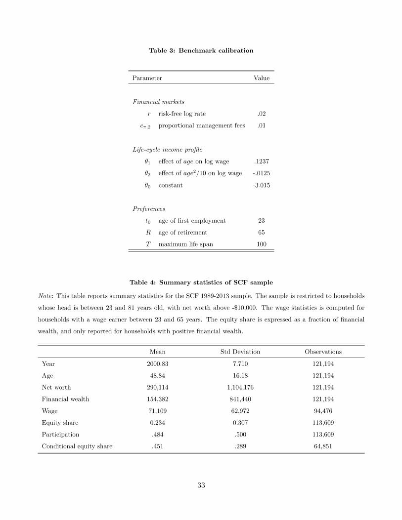
Table 3: Benchmark calibration

Parameter Value

Financial markets

r risk-free log rate .02

cπ,2 proportional management fees .01

Life-cycle income profile

θ1 effect of age on log wage .1237

θ2 effect of age2/10 on log wage -.0125

θ0 constant -3.015

Preferences

t0 age of first employment 23

R age of retirement 65

T maximum life span 100

Table 4: Summary statistics of SCF sample

Note: This table reports summary statistics for the SCF 1989-2013 sample. The sample is restricted to households

whose head is between 23 and 81 years old, with net worth above -$10,000. The wage statistics is computed for

households with a wage earner between 23 and 65 years. The equity share is expressed as a fraction of financial

wealth, and only reported for households with positive financial wealth.

Mean Std Deviation Observations

Year 2000.83 7.710 121,194

Age 48.84 16.18 121,194

Net worth 290,114 1,104,176 121,194

Financial wealth 154,382 841,440 121,194

Wage 71,109 62,972 94,476

Equity share 0.234 0.307 113,609

Participation .484 .500 113,609

Conditional equity share .451 .289 64,851

33

Table 5: Estimated parameters: preferences and participation cost

Note: This table reports results of my structural estimation. Panel A shows the estimated parameters and their

standard errors while Panel B indicates which sets of life-cycle moments from the SCF data are targeted. Columns

(1) and (2) assume no fixed participation cost and target the evolution of wealth and of the unconditional equity

share. Columns (3) and (4) include a per period participation cost which is a fraction of the national average

wage and, beside wealth, target the life-cycle profiles of the participation rate and the conditional equity share.

In columns (5) and (6), I introduce a fraction of the population which never participates in the stock market. In

columns (1), (3) and (5), the model takes into account the cyclical skewness of idiosyncratic income shocks, whereas

in columns (2), (4) and (6) labor income shocks are log normally distributed with identical variance, persistence

and covariance with stock returns as in columns (1), (3) and (5). All models include stock market crashes.

With cyclical skewness Without cyclical skewness

(1) (2) (3) (4) (5) (6)

Panel A: Estimated parameters

Relative risk aversion 6.974 5.543 5.274 10.810 6.464 6.501

(.004) (.004) (.003) (.007) (.002) (.004)

Discount factor 0.946 0.890 0.921 0.798 0.955 0.954

(.004) (.006) (.005) (.012) (.004) (.008)

Fixed participation cost 0.006 0.007 0.021 0.020

(.000) (.000) (.000) (.000)

Fraction of never participants 0.233 0.015

(.001) (.001)

Panel B: Targeted life-cycle moments

Wealth

Equity share

Participation rate

Conditional equity share

34

Table 6: Aggregate effect of cyclical skewness on the demand for equity

Note: This table reports the effects of cyclical skewness on the aggregate demand for equity. Using models

(1), (2) and (3) of Table 5, I simulate the life of 106 individuals and sum their equity holdings over all ages,

including retirement. Holding everything else equal, I then remove cyclical skewness from the model and repeat

the computation. The first line of the table reports the log difference in aggregate demand for equity between the

model without and the model with cyclical skewness. The log difference is explained by the change in aggregate

wealth and the change in the aggregate equity share. I also compute the change in the equity premium (in both µ−s

and µ+s ) that exactly offsets the effect of removing cyclical skewness. Specifically, I use Newton’s method to find

the equity premium for which the aggregate demand in the model without cyclical skewness equals the demand in

the model with cyclical skewness and the true equity premium.

Model

(1) (2) (3)

Aggregate effect of cyclical skewness on:

– ln(equity share) -.172 -.205 -.140

– ln(wealth) .039 .054 .048

– ln(demand for equity) -.133 -.151 -.092

Equivalent change in equity premium -.004 -.005 -.004

35

Figure 1: Skewness of income shocks and stock returns in the US

Note: This graph plots the evolution of the cross-sectional skewness of log wage yearly changes (line) in the US

from 1978 to 2010 and yearly S&P500 log returns (bars). Here, skewness is defined as (d9−d5)−(d5−d1)d9−d1 , where di

denotes the ith decile of the log change in wage. Those deciles are computed by Guvenen et al. (2014) using Social

Security panel data. Their sample is restricted to male workers between 25 and 60 years old and log wage changes

are adjusted for life-cycle effects. S&P500 data are taken from Robert Shiller’s website.

1980 1985 1990 1995 2000 2005 2010-0.6

-0.5

-0.4

-0.3

-0.2

-0.1

0

0.1

0.2

0.3

0.4

-0.3

-0.25

-0.2

-0.15

-0.1

-0.05

0

0.05

0.1

0.15

0.2

36

Figure 2: Fitness of idiosyncratic labor income risk model

Note: This figure reports the empirical and simulated values of moments targeted in the estimation of the dynamics

of idiosyncratic labor income shocks. Panels A to E report, for each year, cross-sectional moments from the

distribution of labor income log growth, net of life-cycle effects, at the one, three and five year horizons among US

male salaried workers between 25 and 60 years old. Here, skewness is defined as (d9−d5)−(d5−d1)d9−d1 . Panel F reports the

average historical within-cohort standard deviation of labor income at each age. All these moments are computed

by Guvenen et al. (2014) and Guvenen et al. (2015) using Social Security panel data. I simulate 67 cohorts of 7,500

individuals, with the first cohort entering the labor market in 1944. Historical aggregate income shocks between

1943 and 2010 are exogenous inputs in the simulation and come from Social Security data (1978-2010) and NIPA

tables (1944-1977).

1980 1985 1990 1995 2000 2005 2010-0.3

-0.2

-0.1

0

0.1

0.2

0.3

1980 1985 1990 1995 2000 2005 2010-0.3

-0.2

-0.1

0

0.1

0.2

0.3

1980 1985 1990 1995 2000 2005 2010-0.3

-0.2

-0.1

0

0.1

0.2

0.3

25 30 35 40 45 50 55 600.5

0.6

0.7

0.8

0.9

1

1.1

1980 1985 1990 1995 2000 2005 20100.4

0.5

0.6

0.7

0.8

0.9

1980 1985 1990 1995 2000 2005 20100.4

0.5

0.6

0.7

0.8

0.9

37

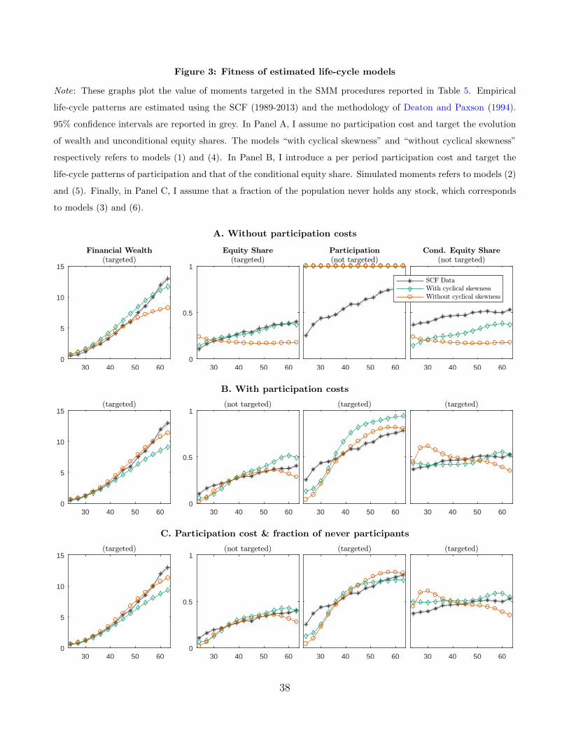
Figure 3: Fitness of estimated life-cycle models

Note: These graphs plot the value of moments targeted in the SMM procedures reported in Table 5. Empirical

life-cycle patterns are estimated using the SCF (1989-2013) and the methodology of Deaton and Paxson (1994).

95% confidence intervals are reported in grey. In Panel A, I assume no participation cost and target the evolution

of wealth and unconditional equity shares. The models “with cyclical skewness” and “without cyclical skewness”

respectively refers to models (1) and (4). In Panel B, I introduce a per period participation cost and target the

life-cycle patterns of participation and that of the conditional equity share. Simulated moments refers to models (2)

and (5). Finally, in Panel C, I assume that a fraction of the population never holds any stock, which corresponds

to models (3) and (6).

A. Without participation costs

30 40 50 600

5

10

15

30 40 50 600

0.5

1

30 40 50 60 30 40 50 60

B. With participation costs

30 40 50 600

5

10

15

30 40 50 600

0.5

1

30 40 50 60 30 40 50 60

C. Participation cost & fraction of never participants

30 40 50 600

5

10

15

30 40 50 600

0.5

1

30 40 50 60 30 40 50 60

38

Fig

ure

4:

Op

tim

al

equ

ity

share

at

40

wit

hou

tp

art

icip

ati

on

cost

Note

:T

his

figu

rere

pre

sents

the

opti

mal

equ

ity

share

for

a40

yea

rsold

work

er,

wh

ose

mea

nh

isto

rica

lta

xab

lew

age

has

bee

nS

=1

sofa

r,as

afu

nct

ion

oftw

ost

ate

vari

able

s:th

elo

gsof

her

fin

an

cial

wea

lthx

an

dth

elo

gof

her

per

sist

ent

inco

mez.

Th

etr

an

sito

ryp

art

of

inco

me

isze

ro.

Wea

lth

and

per

sist

ent

inco

me

are

scal

edby

the

nati

on

al

wage

ind

ex.

The

part

icip

ati

on

cost

isse

tto

zero

.In

pan

elA

,all

mod

elp

ara

met

ers

are

set

toth

eir

ben

chm

ark

valu

es,

and

rep

lica

tes

the

skew

nes

sof

stock

retu

rns

an

dth

ecy

clic

al

skew

nes

sof

idio

syn

crati

cin

com

esh

ock

s.In

pan

elB

,p

ersi

sten

tin

com

esh

ock

sar

elo

gnor

mal

lyd

istr

ibu

ted

wit

hsa

me

per

sist

ence

,va

rian

cean

dco

vari

an

cew

ith

stock

retu

rns

as

inp

an

elA

.S

tock

mark

etd

isas

ters

occ

ur

inb

oth

spec

ifica

tion

s.

1

00.

56

40

0.2

2-0

.5

0.4

0

-1-2

0.6

0.81

1

00.

56

40

0.2

2-0

.5

0.4

0

-1-2

0.6

0.81

39

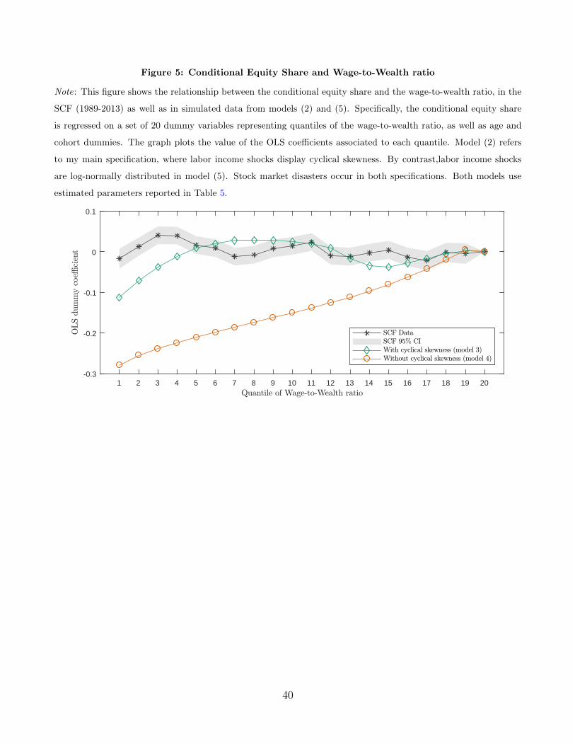
Figure 5: Conditional Equity Share and Wage-to-Wealth ratio

Note: This figure shows the relationship between the conditional equity share and the wage-to-wealth ratio, in the

SCF (1989-2013) as well as in simulated data from models (2) and (5). Specifically, the conditional equity share

is regressed on a set of 20 dummy variables representing quantiles of the wage-to-wealth ratio, as well as age and

cohort dummies. The graph plots the value of the OLS coefficients associated to each quantile. Model (2) refers

to my main specification, where labor income shocks display cyclical skewness. By contrast,labor income shocks

are log-normally distributed in model (5). Stock market disasters occur in both specifications. Both models use

estimated parameters reported in Table 5.

1 2 3 4 5 6 7 8 9 10 11 12 13 14 15 16 17 18 19 20-0.3

-0.2

-0.1

0

0.1

40

Figure 6: Decomposition of effects on the equity share

Note: These graphs plot the simulated life-cycle profile of the equity share under different scenarios. In Scenario

(a), log returns and idiosyncratic income shocks are normally distributed. In scenario (b), I introduce stock market

crashes. Scenario (c) incorporates the cyclical skewness of income shocks but assumes that log returns are normally

distributed. Scenario (d) combines the effects of stock market crashes and cyclical skewness. Returns, transitory

and persistent income shocks have identical means, variances and covariances in all scenarios.

25 30 35 40 45 50 55 60 650

0.2

0.4

0.6

0.8

1

25 30 35 40 45 50 55 60 65

Figure 7: Effect of Social Security

Note: These graphs plot the life-cycle profiles of financial wealth, equity holdings and the unconditional equity

share in the benchmark calibration, in the presence of participation costs, with and without Social Security. In

the absence of Social Security, the agent does not receive any pension nor pay payroll taxes. Financial wealth and

equity holdings are scaled by the national average wage.

25 30 35 40 45 50 55 60 650

5

10

15

20

25

25 30 35 40 45 50 55 60 650

2

4

6

25 30 35 40 45 50 55 60 650

0.2

0.4

0.6

0.8

1

41

Figure 8: Decomposition of countercyclical consumption risk by deciles of wealth and age

Note: This graph plots the relative contribution of each decile of wealth and age to the cyclical skewness of

consumption growth in the simulated data. Cyclicality is measured using cokurtosis, defined in equation (21).

Using estimated parameters reported in column (2) of Table 5, I simulate the life-cycle of 106 individuals, including

retirement. Simulated data are split by deciles of financial wealth (left panel) and deciles of age (right panel). The

graph reports the relative contribution of each decile to the total cokurtosis and total financial wealth.

1 2 3 4 5 6 7 8 9 100

0.1

0.2

0.3

0.4

0.5

1 2 3 4 5 6 7 8 9 10

42

Figure 9: Sensitivity of π to risk aversion

Note: These graphs plot the evolution of the mean equity share over the life-cycle for different levels of relative risk

aversion. In the “no effect” scenario, log returns and income shocks are normally distributed with same variance,

covariance and persistence as in the model with cyclical skewness and stock market crashes (“all effects”).

A. Without participation cost

20 35 50 650

0.5

1

20 35 50 65 20 35 50 65 20 35 50 65 20 35 50 65

B. With participation cost

20 35 50 650

0.5

1

20 35 50 65 20 35 50 65 20 35 50 65 20 35 50 65

43

INTERNET APPENDIX

A Stock market returns and labor income risk

A.1 Idiosyncratic shocks

This section details the parametric estimation of the idiosyncratic income risk process. I largely follow the method-

ology of Guvenen et al. (2014) and detailed in their own appendix. I target the following moments: the standard

deviation of log income changes at the 1 and 5 year horizons, and Kelly’s skewness of log income changes at the 1,

3 and 5 year horizons for each year between 1978 and 2010. There are two differences in targeted moments. First,

I do not include the mean, which, in my paper, is generated by another process. Since I focus on idiosyncratic

shocks, the mean is subtracted from the moments provided by Guvenen et al. (2014). Second, I target the evolution

of within-cohorts inequalities (standard deviation of log-income) between 25 and 60 years old, in order to control

for the existence of individual fixed-effects in income growth rates. This last set of moment is taken from Guvenen

et al. (2015). In total, I target 191 moments.

For each moment mt of the skewness and standard deviation times series, the distance between the empirical

moment and the simulated one is normalized. Specifically, the distance d is computed as:

dmt(Φ) =

mt,data −mt,simu(Φ)

mdata(22)

where Φ is a vector of parameters and mdata is the historical mean of the absolute value of moment m.

For life-cycle inequalities, I compute the standard deviation for each age/year, and take the average across years.

The result is the historical standard deviation of log income for each age. The distance between the simulation and

the target is simply

dm(Φ) =mdata −msimu(Φ)

mdata(23)

The weighting matrix Ω is diagonal and weights are chosen so that 3/4 of the total is given to the skewness

and standard deviation of income changes and the remaining to life-cycle inequalities. Within each of these two

groups of moments, all targets receive equal weights. As in Guvenen et al. (2014), the simulation starts in 1944 to

maintain a constant age structure and each individual reaching 60 is replaced by a young worker.Aggregate income

shocks before 1978 are derived from NIPA tables12. Each cohort includes 1, 000 individuals, which means that at

12This time-series is borrowed from Emmanuel Saez’ website: http://eml.berkeley.edu/∼saez/TabFig2012prel.xls

44

http://eml.berkeley.edu/~saez/TabFig2012prel.xls

any time the economy is occupied by 36, 000 workers. The goal of the SMM is to minimize

minΦd(Φ)′Ωd(Φ) (24)

where d(Φ) is a vector composed of the values of dm(Φ) for all moments m.

The optimization is done in two steps. In the first stage, I generate 105 quasi-random vectors of parameters

from a Halton sequence and evaluate the value function for each of them. In the second step, I use the Nelder-Mead

method to perform a local optimization using the best 2, 000 results from the first stage as starting points. Like

GOS, I simulate several (5) economies and averages moments accross these economies in order to smooth the surface

of the objective function.

A.2 Macroeconomic shocks

The SMM used to estimate the macroeconomic risk model is straightforward. I minimize the sum of the distances,

measured in percentage as in equation (23). All moments are nearly matched by using the identity matrix.

B Numerical resolution of the model

B.1 Grid design

The state and control variables of the problem are discretized as follows. Financial wealth X is measured in national

wages and takes values between 0.01 and 200. The grid is uniformly distributed between the logs of these two values

with a mesh size of ∆(x) = .025. The persistent component of wage takes uniformly distributed values between

−3 and 3, that is .05 and 20 the national wage index, with a mesh size of ∆(z) = .05. Similarly, the transitory

component can take 41 equally distributed values between minus two and two standard deviations. Social Security

entitlements are measured in terms of b, the percentage of the national wage that the agent would get as benefit if

he had 65 years old. The upper bound of the grid is the upper limit of this percentage given Social Security rules.

The lower bound is 0.001 and the mesh size ∆ (b(S)) = .03. Consumption is defined as a position between two

bounds. I define minimum and maximum consumption such that the agent stays within the grid and has positive

consumption. She chooses consumption on a grid that spans over this interval. The grid is constructed using the

log of consumption with of a mesh size ∆(x) = .01. Finally, the equity share can take 101 equally spaced values

between 0 and 1.

This discretization generates a grid of considerable size. I detail how the problem is solved in the following

sub-sections.

– Table B1.

45

B.2 Discretization of stochastic processes

Three state variables of the problem have a stochastic dynamics: η, z, and x.

Transitory income shocks — The dynamics of η is discretized assuming that

Pd(ηt = η) = P

(ηt = η ± ∆(η)

2

)(25)

where η is a point on the grid of η and P and Pd are respectively the continuous and discretized probability.

Wealth and persistent income — The discretization of the joint dynamics of x and z requires a more

specific methodology due to several difficulties.

First, a transition matrix must be computed for each possible value of π. Moreover, each of these 101 matrices

would include 450 × 121 × 450 × 121 ≈ 3 × 109 elements. To alleviate this dimensionality problem, I use the fact

that P (xt+1 = x1 + δx|xt = x1, π) = P (xt+1 = x2 + δx|xt = x2, π) to compute the transition matrix for only one

value of xt. I also use the fact that the transition matrix of xt to xt+1 is a band matrix (when extremely small

probabilities are rounded to zero) to restrict variations in x to ±.75, which corresponds to ± 25 grid points. As a

result, to each value of π corresponds a transition matrix of 121× 51× 121 ≈ 7.5× 105 elements.

The second difficulty is the non-trivial relationship between x and z: shocks to x are correlated with δl,t, which

in turn determines parameters of the distribution of z. Finally, following equation (18), the value function must

be adjusted for variations in the scaling state variable l. I circumvent the last two difficulties using the following

method:

1. In a first step, I discretize δl using a grid of 101 points uniformly distributed between −.15 and .15. I then

compute the transition matrix from xt to (xt+1,δl,t). Since these two random variables are correlated in a

trivial way, the discretized probability of any pair (x, δl) on the grid can be approximated using the following

rule:

Pd(xt+1 = x ∩ δl,t = δl|xt, π) = P

(xt+1 = x± ∆(x)

2

⋂δl,t = δl ±

∆(δl)

2

∣∣∣∣xt, π) (26)

where ∆(δl) the distance between two grid points.

2. In a second step, I compute the transition matrix of z for each value of the grid of δl. Each component of

the mixture is discretized using the Tauchen method (Tauchen (1986)). The transition matrix of z is the

weighted sum of the transition matrices associated with the two components of the mixture.

3. Finally, one can then use the law of total probability along the δl dimension to compute the joint transition

matrix of x and z. Specifically, for any pair (x, z) on the grid, we have

Pd(xt+1 = x ∩ zt+1 = z|xt, zt, π) =∑δl

Pd(xt+1 = x ∩ δl,t = δl|xt, π)

×Pd(zt+1 = z|zt, δl)(27)

However, because I need to take into account how variations in l affect the value function of the agent, I

46

actually use an adjusted version of equation (27):

Pd(xt+1 = x ∩ zt+1 = z|xt, zt, π) =∑δl

Pd(xt+1 = x ∩ δl,t = δl|xt, π)

×Pd(zt+1 = z|zt, δl)e(1−γ)δl(28)

As a result of the positive drift of l, this formula implies that the rows of the transition matrix sum to a

number slightly below one.

B.3 Resolution of the Bellman equation

The model is solved by dynamic programming. Each year is split into two sub-periods. In the first sub-period, the

agent receives her transitory income shock, receives her wage and decides how much to consume. In the second sub-

period, she decides how to invest her remaining wealth, and then receives shocks to her wealth and her persistent

income. Following the logic of backward induction, the two sub-periods are solved in reverse order.

Consumption sub-period — For a given consumption, the continuation value of the agent is determined

by the new value of x and the new value of b, which depends on her current wage and income record.

Portfolio choice sub-period — In the second period, the agent chooses her equity share by maximizing

her expected utility. In this period, I need to extrapolate the value function along the x dimension because equity

returns can move the agent across the borders of the grid. This has little practical consequences since the wealth grid

spans from 0.01 to 200 national wages. Transitory and persistent income shocks happen in different sub-periods,

even though the same Bernoulli variable determines which component of their respective mixtures is received by

the agent. To solve this problem, I keep track of this Bernoulli variable. Although this method multiplies the state

space by two, it remains much less computationally intensive than using a joint transition matrix of z, x and η.

Extrapolation methodology — The negative of the value function is of the Cobb-Douglas form and

therefore log-linear with respect to the log of consumption. To take advantage of this property, I use log-linear

extrapolations of the negative of V , and then take the negative of the exponential of the result to retrieve the

extrapolated value function.

Retirement period — Retirement years may be seen as degenerated working years, where state variables z

and η become irrelevant. Yet, because benefits are no longer wage indexed, the value function is no longer scalable

by the national wage. To avoid unnecessary complications, I simply assume a fixed wage index during retirement.

The only economic shortcoming of this assumption is to freeze the dollar value of fixed participation costs for

retirees.

B.4 Simulated Method of Moments

The SMM procedure follows the same global optimization routine as the one described in appendix section A.1.

In the first (global) stage, I test 2,000 quasi-randoms vectors of parameters. In the second stage, I run 10 local

47

optimization around the best points of the first stage. I check that the local optimizations converge to the same

point and take it as evidence of a global minimum.

To compute moments, I simulate a sample of 3 × 105 individuals, each receiving different idiosyncratic and

macroeconomic shocks. As a results, there is no cohort and year effects in the simulated data. The predicted equity

share for a given age group is simply the mean among all individuals in that age group. The same logic applies for

wealth, participation and the conditional equity share.

The standard errors are estimated by computing the Jacobian matrix J of the moments with respect to

estimated parameters. The standard errors are the square roots of the diagonal elements of matrix Q, which is

defined as:

Q =[JTWJ

]−1(29)

48

Countercyclical Labor Income Risk and Portfolio Choices ...

Documents