Coulomb stress changes and aftershocks of recent Indian earthquakes

REVIEW ARTICLES

CURRENT SCIENCE, VOL. 88, NO. 4, 25 FEBRUARY 2005 576

*For correspondence. (e-mail: [email protected])

Coulomb stress changes and aftershocks of recent Indian earthquakes Shikha Rajput, V. K. Gahalaut* and Vipul K. Sahu National Geophysical Research Institute, Uppal Road, Hyderabad 500 007, India

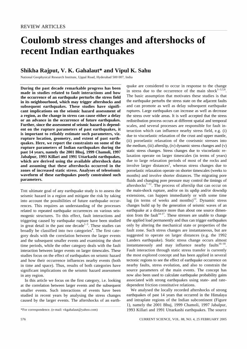
During the past decade remarkable progress has been made in studies related to fault interactions and how the occurrence of an earthquake perturbs the stress field in its neighbourhood, which may trigger aftershocks and subsequent earthquakes. These studies have signifi-cant implications on the seismic hazard assessment of a region, as the change in stress can cause either a delay or an advance in the occurrence of future earthquakes. Further, since the assessment of seismic hazard is depend-ent on the rupture parameters of past earthquakes, it is important to reliably estimate such parameters, viz. rupture location, geometry, and extent of past earth-quakes. Here, we report the constraints on some of the rupture parameters of Indian earthquakes during the past 14 years, namely the 2001 Bhuj, 1999 Chamoli, 1997 Jabalpur, 1993 Killari and 1991 Uttarkashi earthquakes, which are derived using the available aftershock data and assuming that these aftershocks occurred in the zones of increased static stress. Analyses of teleseismic waveform of these earthquakes poorly constrained such parameters.

THE ultimate goal of any earthquake study is to assess the seismic hazard in a region and mitigate the risk by taking into account the possibilities of future earthquake occur-rences. This requires an understanding of the processes related to repeated earthquake occurrences on various seis-mogenic structures. To this effect, fault interactions and triggering caused by earthquake rupture have been studied in great detail in the past one decade1–3. These studies can broadly be classified into two categories4. The first cate-gory deals with the correlation between the larger events and the subsequent smaller events and examining the short time periods, while the other category deals with the fault interaction between larger events on larger timescales. These studies focus on the effect of earthquakes on seismic hazard and how their occurrence influences nearby events (both in time and space). Thus, results of both categories have significant implications on the seismic hazard assessment in any region. In this article we focus on the first category, i.e. looking at the correlation between larger events and the subsequent smaller events. Such interactions of events have been studied in recent years by analysing the stress changes caused by the larger events. The aftershocks of an earth-

quake are considered to occur in response to the change in stress due to the occurrence of the main shock1–3,5,6. The basic assumption that motivates these studies is that the earthquake perturbs the stress state on the adjacent faults and can promote as well as delay subsequent earthquake ruptures. Large earthquakes can increase as well as decrease the stress over wide areas. It is well accepted that the stress redistribution process occurs at different spatial and temporal scales, and several processes are responsible for fault in-teraction which can influence nearby stress field, e.g. (i) due to viscoelastic relaxation of the crust and upper mantle, (ii) poroelastic relaxation of the coseismic stresses into the medium, (iii) afterslip, (iv) dynamic stress changes and (v) static stress changes. Stress changes due to viscoelastic re-laxation operate on larger timescales (in terms of years) due to large relaxation periods of most of the rocks and involve larger distances2, whereas stress changes due to poroelastic relaxation operate on shorter timescales (weeks to months) and involve shorter distances. The migrating pore fluids and changing pore pressure may control the timings of aftershocks7–12. The process of afterslip that can occur on the main-shock rupture, and/or on its updip and/or downdip extensions, can happen immediately or with some time lag (in terms of weeks and months)13. Dynamic stress changes build up by the generation of seismic waves of an earthquake at a distance more than about one source dimen-sion from the fault14–17. These stresses are unable to change the applied load permanently and thus can trigger earthquakes only by altering the mechanical state or properties of the fault zone. Such stress changes are instantaneous, but are suggested to operate on larger distances (e.g. the 1992 Landers earthquake). Static stress change occurs almost instantaneously and may influence nearby faults16–18. Fault interaction through static stress transfer is currently the most explored concept and has been applied in several tectonic regions to see the effect of earthquake occurrence on nearby faults, stress evolution, and also to constrain the source parameters of the main events. The concept has now also been used to calculate earthquake probability gains associated with strong earthquakes using state- and rate-dependent friction constitutive relations. We analysed the locally recorded aftershocks of strong earthquakes of past 14 years that occurred in the Himalaya and intraplate regions of the Indian subcontinent (Figure 1), namely the 2001 Bhuj, 1999 Chamoli, 1997 Jabalpur, 1993 Killari and 1991 Uttarkashi earthquakes. The source

REVIEW ARTICLES


parameters of these earthquakes are either not known or poorly constrained using either the far-field earthquake waveforms or near-field strong motion data. In view of the worldwide studies suggesting good correlation between the zone of aftershocks and increased static stress changes, we test this hypothesis and investigate whether it can broadly constrain some of the source parameters of these earthquakes. The analyses of the 1993 Killari and 1997 Jabalpur earthquakes are already published19,20. However, for the sake of completeness, we briefly review them here. Analyses of the 1991 Uttarkashi, 1999 Chamoli and 2001 Bhuj earthquakes are reported here. We assume that the aftershocks of these earthquakes occurred due to a change in regional stress, which is caused by the coseismic static stress change due to the main earthquake. Thus spatial variation in the aftershocks helped in constraining some of the source parameters of the earthquakes.

Concept of static stress

Various methods have been used to explain the conditions under which failure occurs in rocks. Coulomb failure method is one of the more widely used methods. It is based on the assumption that majority of aftershocks of large earthquakes occur in the regions of increased Coulomb static stress change ∆Sf, which is defined as1,2,5,6,21

Figure 1. Epicentres of five earthquakes, namely the 2001 Bhuj, 1999 Chamoli, 1997 Jabalpur, 1993 Killari (Latur) and 1991 Uttarkashi earthquakes, that are analysed here for providing the constraints on the rupture parameters, shown over the smooth topography.

∆Sf = ∆τ – µ ′∆σ, where ∆τ and ∆σ are the static shear stress changes (assumed positive in the direction of fault slip) and effective normal stress changes (positive if compressive) on the fault plane caused by the main shock respectively, while µ ′ is the effec-tive coefficient of friction defined as µ ′ = µ(1–B), where B is the Skempton’s coefficient whose value lies between 0 and 1. The stress changes in an elastic half-space due to slip on a rectangular fault are computed using21 Coulomb 2.5. For all the earthquakes discussed here a shear modulus of 3.2 × 105 bar and a Poisson ratio5 of 0.25 are assumed. Throughout our analyses, we assumed σ1 to be sub-horizontal in the NNE direction, which is in general consistent with the Indian plate motion22,23 and focal mechanisms of the earthquakes considered here. Failure is encouraged if ∆Sf is positive, and discouraged if it is negative. Thus it is consid-ered that the aftershocks generally occur in the zone of in-creased ∆Sf. It has been demonstrated that changes of Coulomb stress ranging between 0.1 and 1 bar (sometimes even smaller as 0.01 bar) can influence the occurrence of future earth-quakes. This seems surprising because stress drops of an earthquake are commonly much larger, e.g. several bars to several hundred bars. Hence such a small change in static stress might be too small to affect any crustal fault. It must be noted that ∆Sf cannot produce earthquakes, it can only trigger an earthquake. In this situation, the fault is assumed to be sufficiently close to the failure state due to the natural tectonic process and only a small stress pertur-bation is sufficient to produce or enhance the instability.

The 2001 Bhuj earthquake

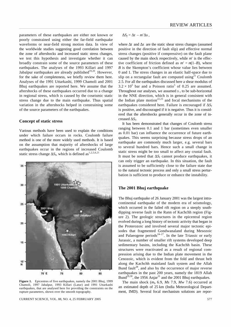
The Bhuj earthquake of 26 January 2001 was the largest intra-continental earthquake of the modern era of seismology, which occurred in the failed rift region on a steeply south-dipping reverse fault in the Rann of Kachchh region (Fig-ure 2). The geologic structures in the epicentral region evolved during a long history of tectonic activity that began in the Proterozoic and involved several major tectonic epi-sodes that fragmented Gondwanaland during Mesozoic and Palaeogene periods24–27. In the late Triassic or early Jurassic, a number of smaller rift systems developed deep sedimentary basins, including the Kachchh basin. These structures were reactivated as a result of regional com-pression arising due to the Indian plate movement in the Cenozoic, which is evident from the fold and thrust belt along the Kachchh mainland fault system and the Allah Bund fault28, and also by the occurrence of major reverse earthquakes in the past 200 years, namely the 1819 Allah Bund29,30, the 1956 Anjar31 and the 2001 Bhuj earthquakes. The main shock (mb 6.9, Ms 7.9, Mw 7.6) occurred at an estimated depth of 25 km (India Meteorological Depart-ment, IMD). Several focal mechanism solutions are repor-

REVIEW ARTICLES


ted32, which suggest predominantly reverse motion on a steeply south-dipping (51–66°) fault. Antolik and Dreger33 reported a focal mechanism solution on the basis of far-field waveform modelling (Figure 2). We used their focal mechanism solution in our analysis (NP1: 82°, 51°, 77°). Thus the earthquake occurred in the lower crust on a steeply dipping reverse fault and the rupture did not extend up to the surface, or project towards a mapped surface fault.

Aftershocks of the 2001 Bhuj earthquake

We used aftershock data of this earthquake as reported by Negishi et al.34. They operated a seven-station three-component digital station network, which was in operation from 28 February to 6 March 2001. They located 1428 after-shocks using joint hypocentre determination programme35 (Figure 2). The root mean square error in the travel time is of the order of 0.02–0.07 s. The aftershock trend is consistent with the dip of rupture as 50°. Most of the after-shocks occurred at depths between 10 and 35 km.

Analysis and results

Antolik and Dreger33 inverted teleseismic broadband body waves of the 2001 Bhuj earthquake. They estimated the focal mechanism and the slip distribution on the rupture for this earthquake. Though they reported that significant slip occurred at shallow depth (0–10 km), it was not well resolved. Field investigations after the earthquake reported no evidence of surface faulting32. Gahalaut and Bürgmann36 reported that rupture in updip direction extended up to a depth of 10 km only. Thus, to calculate the change in static

Figure 2. Generalized structural map of Kachchh24,28. PU, Pachchham uplift; KU, Khader uplift; BU, Bela uplift. Aftershocks34 of the 2001 Bhuj earthquake (epicentre shown by star), focal mechanism of the main earthquake33 and inferred rupture are also shown.

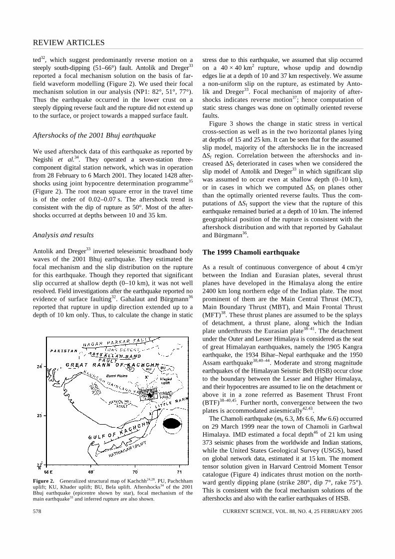
stress due to this earthquake, we assumed that slip occurred on a 40 × 40 km2 rupture, whose updip and downdip edges lie at a depth of 10 and 37 km respectively. We assume a non-uniform slip on the rupture, as estimated by Anto-lik and Dreger33. Focal mechanism of majority of after-shocks indicates reverse motion37; hence computation of static stress changes was done on optimally oriented reverse faults. Figure 3 shows the change in static stress in vertical cross-section as well as in the two horizontal planes lying at depths of 15 and 25 km. It can be seen that for the assumed slip model, majority of the aftershocks lie in the increased ∆Sf region. Correlation between the aftershocks and in-creased ∆Sf deteriorated in cases when we considered the slip model of Antolik and Dreger33 in which significant slip was assumed to occur even at shallow depth (0–10 km), or in cases in which we computed ∆Sf on planes other than the optimally oriented reverse faults. Thus the com-putations of ∆Sf support the view that the rupture of this earthquake remained buried at a depth of 10 km. The inferred geographical position of the rupture is consistent with the aftershock distribution and with that reported by Gahalaut and Bürgmann36.

The 1999 Chamoli earthquake

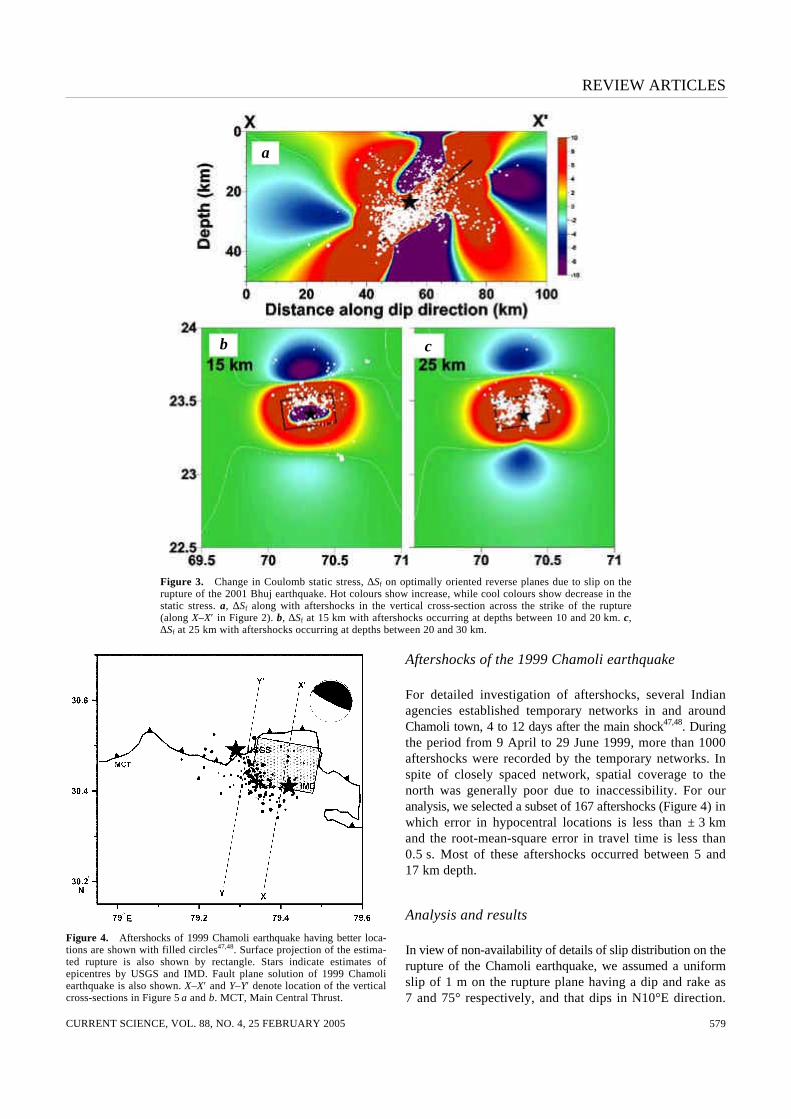
As a result of continuous convergence of about 4 cm/yr between the Indian and Eurasian plates, several thrust planes have developed in the Himalaya along the entire 2400 km long northern edge of the Indian plate. The most prominent of them are the Main Central Thrust (MCT), Main Boundary Thrust (MBT), and Main Frontal Thrust (MFT)38. These thrust planes are assumed to be the splays of detachment, a thrust plane, along which the Indian plate underthrusts the Eurasian plate38–41. The detachment under the Outer and Lesser Himalaya is considered as the seat of great Himalayan earthquakes, namely the 1905 Kangra earthquake, the 1934 Bihar–Nepal earthquake and the 1950 Assam earthquake38,40–44. Moderate and strong magnitude earthquakes of the Himalayan Seismic Belt (HSB) occur close to the boundary between the Lesser and Higher Himalaya, and their hypocentres are assumed to lie on the detachment or above it in a zone referred as Basement Thrust Front (BTF)38–40,45. Further north, convergence between the two plates is accommodated asiesmically42,43. The Chamoli earthquake (mb 6.3, Ms 6.6, Mw 6.6) occurred on 29 March 1999 near the town of Chamoli in Garhwal Himalaya. IMD estimated a focal depth46 of 21 km using 373 seismic phases from the worldwide and Indian stations, while the United States Geological Survey (USGS), based on global network data, estimated it at 15 km. The moment tensor solution given in Harvard Centroid Moment Tensor catalogue (Figure 4) indicates thrust motion on the north-ward gently dipping plane (strike 280°, dip 7°, rake 75°). This is consistent with the focal mechanism solutions of the aftershocks and also with the earlier earthquakes of HSB.

REVIEW ARTICLES


Figure 3. Change in Coulomb static stress, ∆Sf on optimally oriented reverse planes due to slip on the rupture of the 2001 Bhuj earthquake. Hot colours show increase, while cool colours show decrease in the static stress. a, ∆Sf along with aftershocks in the vertical cross-section across the strike of the rupture (along X–X′ in Figure 2). b, ∆Sf at 15 km with aftershocks occurring at depths between 10 and 20 km. c, ∆Sf at 25 km with aftershocks occurring at depths between 20 and 30 km.

Figure 4. Aftershocks of 1999 Chamoli earthquake having better loca-tions are shown with filled circles47,48. Surface projection of the estima-ted rupture is also shown by rectangle. Stars indicate estimates of epicentres by USGS and IMD. Fault plane solution of 1999 Chamoli earthquake is also shown. X–X′ and Y–Y′ denote location of the vertical cross-sections in Figure 5 a and b. MCT, Main Central Thrust.

Aftershocks of the 1999 Chamoli earthquake

For detailed investigation of aftershocks, several Indian agencies established temporary networks in and around Chamoli town, 4 to 12 days after the main shock47,48. During the period from 9 April to 29 June 1999, more than 1000 aftershocks were recorded by the temporary networks. In spite of closely spaced network, spatial coverage to the north was generally poor due to inaccessibility. For our analysis, we selected a subset of 167 aftershocks (Figure 4) in which error in hypocentral locations is less than ± 3 km and the root-mean-square error in travel time is less than 0.5 s. Most of these aftershocks occurred between 5 and 17 km depth.


In view of non-availability of details of slip distribution on the rupture of the Chamoli earthquake, we assumed a uniform slip of 1 m on the rupture plane having a dip and rake as 7 and 75° respectively, and that dips in N10°E direction.

b c

a

REVIEW ARTICLES


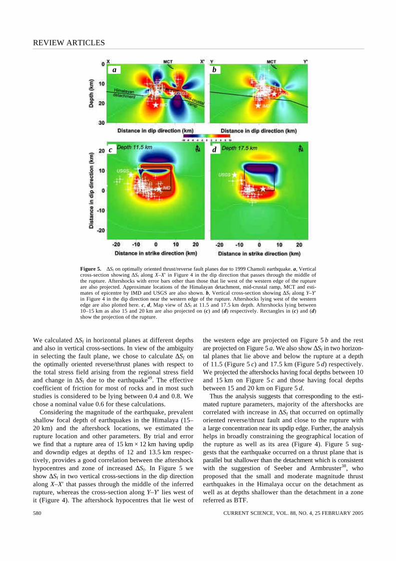
Figure 5. ∆Sf on optimally oriented thrust/reverse fault planes due to 1999 Chamoli earthquake. a, Vertical cross-section showing ∆Sf along X–X′ in Figure 4 in the dip direction that passes through the middle of the rupture. Aftershocks with error bars other than those that lie west of the western edge of the rupture are also projected. Approximate locations of the Himalayan detachment, mid-crustal ramp, MCT and esti-mates of epicentre by IMD and USGS are also shown. b, Vertical cross-section showing ∆Sf along Y–Y′ in Figure 4 in the dip direction near the western edge of the rupture. Aftershocks lying west of the western edge are also plotted here. c, d, Map view of ∆Sf at 11.5 and 17.5 km depth. Aftershocks lying between 10–15 km as also 15 and 20 km are also projected on (c) and (d) respectively. Rectangles in (c) and (d) show the projection of the rupture.

We calculated ∆Sf in horizontal planes at different depths and also in vertical cross-sections. In view of the ambiguity in selecting the fault plane, we chose to calculate ∆Sf on the optimally oriented reverse/thrust planes with respect to the total stress field arising from the regional stress field and change in ∆Sf due to the earthquake49. The effective coefficient of friction for most of rocks and in most such studies is considered to be lying between 0.4 and 0.8. We chose a nominal value 0.6 for these calculations. Considering the magnitude of the earthquake, prevalent shallow focal depth of earthquakes in the Himalaya (15–20 km) and the aftershock locations, we estimated the rupture location and other parameters. By trial and error we find that a rupture area of 15 km × 12 km having updip and downdip edges at depths of 12 and 13.5 km respec-tively, provides a good correlation between the aftershock hypocentres and zone of increased ∆Sf. In Figure 5 we show ∆Sf in two vertical cross-sections in the dip direction along X–X′ that passes through the middle of the inferred rupture, whereas the cross-section along Y–Y′ lies west of it (Figure 4). The aftershock hypocentres that lie west of

the western edge are projected on Figure 5 b and the rest are projected on Figure 5 a. We also show ∆Sf in two horizon-tal planes that lie above and below the rupture at a depth of 11.5 (Figure 5 c) and 17.5 km (Figure 5 d) respectively. We projected the aftershocks having focal depths between 10 and 15 km on Figure 5 c and those having focal depths between 15 and 20 km on Figure 5 d. Thus the analysis suggests that corresponding to the esti-mated rupture parameters, majority of the aftershocks are correlated with increase in ∆Sf that occurred on optimally oriented reverse/thrust fault and close to the rupture with a large concentration near its updip edge. Further, the analysis helps in broadly constraining the geographical location of the rupture as well as its area (Figure 4). Figure 5 sug-gests that the earthquake occurred on a thrust plane that is parallel but shallower than the detachment which is consistent with the suggestion of Seeber and Armbruster38, who proposed that the small and moderate magnitude thrust earthquakes in the Himalaya occur on the detachment as well as at depths shallower than the detachment in a zone referred as BTF.

a b

c d

REVIEW ARTICLES


In this regard we recall that a limited attempt to calculate the stress changes due to the 1999 Chamoli earthquake was made by Chander and Sharma50. However, they used the aftershocks reported by USGS, which contain large loca-tion errors. Hence the analysis and results of that exercise are not robust.

The 1997 Jabalpur earthquake

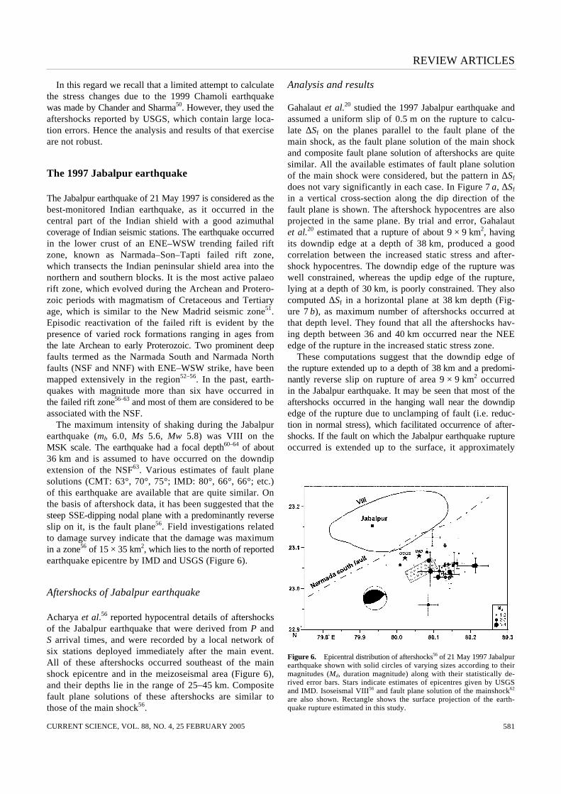
The Jabalpur earthquake of 21 May 1997 is considered as the best-monitored Indian earthquake, as it occurred in the central part of the Indian shield with a good azimuthal coverage of Indian seismic stations. The earthquake occurred in the lower crust of an ENE–WSW trending failed rift zone, known as Narmada–Son–Tapti failed rift zone, which transects the Indian peninsular shield area into the northern and southern blocks. It is the most active palaeo rift zone, which evolved during the Archean and Protero-zoic periods with magmatism of Cretaceous and Tertiary age, which is similar to the New Madrid seismic zone51. Episodic reactivation of the failed rift is evident by the presence of varied rock formations ranging in ages from the late Archean to early Proterozoic. Two prominent deep faults termed as the Narmada South and Narmada North faults (NSF and NNF) with ENE–WSW strike, have been mapped extensively in the region52–56. In the past, earth-quakes with magnitude more than six have occurred in the failed rift zone56–63 and most of them are considered to be associated with the NSF. The maximum intensity of shaking during the Jabalpur earthquake (mb 6.0, Ms 5.6, Mw 5.8) was VIII on the MSK scale. The earthquake had a focal depth60–64 of about 36 km and is assumed to have occurred on the downdip extension of the NSF63. Various estimates of fault plane solutions (CMT: 63°, 70°, 75°; IMD: 80°, 66°, 66°; etc.) of this earthquake are available that are quite similar. On the basis of aftershock data, it has been suggested that the steep SSE-dipping nodal plane with a predominantly reverse slip on it, is the fault plane56. Field investigations related to damage survey indicate that the damage was maximum in a zone56 of 15 × 35 km2, which lies to the north of reported earthquake epicentre by IMD and USGS (Figure 6).

Aftershocks of Jabalpur earthquake

Acharya et al.56 reported hypocentral details of aftershocks of the Jabalpur earthquake that were derived from P and S arrival times, and were recorded by a local network of six stations deployed immediately after the main event. All of these aftershocks occurred southeast of the main shock epicentre and in the meizoseismal area (Figure 6), and their depths lie in the range of 25–45 km. Composite fault plane solutions of these aftershocks are similar to those of the main shock56.


Gahalaut et al.20 studied the 1997 Jabalpur earthquake and assumed a uniform slip of 0.5 m on the rupture to calcu-late ∆Sf on the planes parallel to the fault plane of the main shock, as the fault plane solution of the main shock and composite fault plane solution of aftershocks are quite similar. All the available estimates of fault plane solution of the main shock were considered, but the pattern in ∆Sf does not vary significantly in each case. In Figure 7 a, ∆Sf in a vertical cross-section along the dip direction of the fault plane is shown. The aftershock hypocentres are also projected in the same plane. By trial and error, Gahalaut et al.20 estimated that a rupture of about 9 × 9 km2, having its downdip edge at a depth of 38 km, produced a good correlation between the increased static stress and after-shock hypocentres. The downdip edge of the rupture was well constrained, whereas the updip edge of the rupture, lying at a depth of 30 km, is poorly constrained. They also computed ∆Sf in a horizontal plane at 38 km depth (Fig-ure 7 b), as maximum number of aftershocks occurred at that depth level. They found that all the aftershocks hav-ing depth between 36 and 40 km occurred near the NEE edge of the rupture in the increased static stress zone. These computations suggest that the downdip edge of the rupture extended up to a depth of 38 km and a predomi-nantly reverse slip on rupture of area 9 × 9 km2 occurred in the Jabalpur earthquake. It may be seen that most of the aftershocks occurred in the hanging wall near the downdip edge of the rupture due to unclamping of fault (i.e. reduc-tion in normal stress), which facilitated occurrence of after-shocks. If the fault on which the Jabalpur earthquake rupture occurred is extended up to the surface, it approximately

Figure 6. Epicentral distribution of aftershocks56 of 21 May 1997 Jabalpur earthquake shown with solid circles of varying sizes according to their magnitudes (Md, duration magnitude) along with their statistically de-rived error bars. Stars indicate estimates of epicentres given by USGS and IMD. Isoseismal VIII56 and fault plane solution of the mainshock62 are also shown. Rectangle shows the surface projection of the earth-quake rupture estimated in this study.

REVIEW ARTICLES


coincides with the NSF, supporting the earlier view63 that the earthquake occurred on the downdip extension of the NSF in the lower crust. The estimated depth of the rupture (30 to 38 km) is consistent with the estimates of focal depth for this earthquake60,62,64,65.

The 1993 Killari earthquake

The 1993 Killari earthquake, also known as the Latur earth-quake (mb 6.3, Ms 6.4, Mw 6.2) of 29 September 1993 oc-curred in the Deccan traps of peninsular India, considered to be a stable continental region, and caused destruction in about 15 km wide area (MM intensity VIII). USGS estimated the epicentre of the main shock at about 12 km west of Killari at a focal depth of 6.8 km, whereas

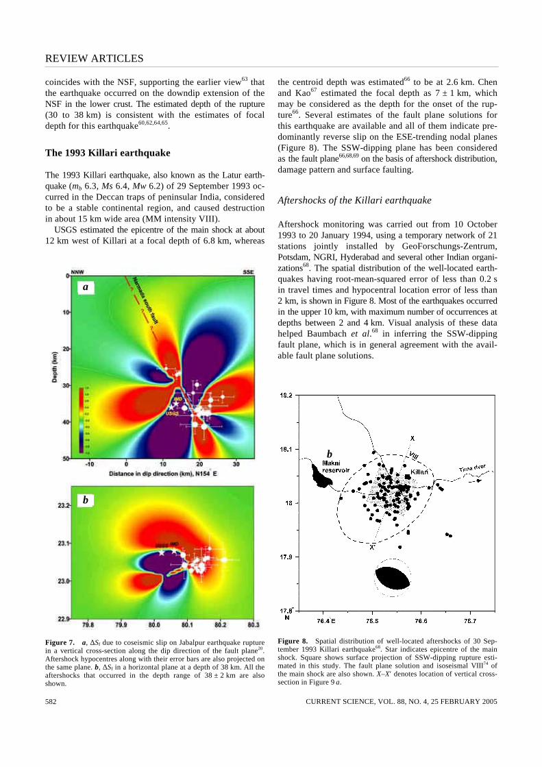
Figure 7. a, ∆Sf due to coseismic slip on Jabalpur earthquake rupture in a vertical cross-section along the dip direction of the fault plane20. Aftershock hypocentres along with their error bars are also projected on the same plane. b, ∆Sf in a horizontal plane at a depth of 38 km. All the aftershocks that occurred in the depth range of 38 ± 2 km are also shown.

the centroid depth was estimated66 to be at 2.6 km. Chen and Kao67 estimated the focal depth as 7 ± 1 km, which may be considered as the depth for the onset of the rup-ture66. Several estimates of the fault plane solutions for this earthquake are available and all of them indicate pre-dominantly reverse slip on the ESE-trending nodal planes (Figure 8). The SSW-dipping plane has been considered as the fault plane66,68,69 on the basis of aftershock distribution, damage pattern and surface faulting.

Aftershocks of the Killari earthquake

Aftershock monitoring was carried out from 10 October 1993 to 20 January 1994, using a temporary network of 21 stations jointly installed by GeoForschungs-Zentrum, Potsdam, NGRI, Hyderabad and several other Indian organi-zations68. The spatial distribution of the well-located earth-quakes having root-mean-squared error of less than 0.2 s in travel times and hypocentral location error of less than 2 km, is shown in Figure 8. Most of the earthquakes occurred in the upper 10 km, with maximum number of occurrences at depths between 2 and 4 km. Visual analysis of these data helped Baumbach et al.68 in inferring the SSW-dipping fault plane, which is in general agreement with the avail-able fault plane solutions.

Figure 8. Spatial distribution of well-located aftershocks of 30 Sep-tember 1993 Killari earthquake68. Star indicates epicentre of the main shock. Square shows surface projection of SSW-dipping rupture esti-mated in this study. The fault plane solution and isoseismal VIII74 of the main shock are also shown. X–X′ denotes location of vertical cross-section in Figure 9 a.

b

b

a

REVIEW ARTICLES



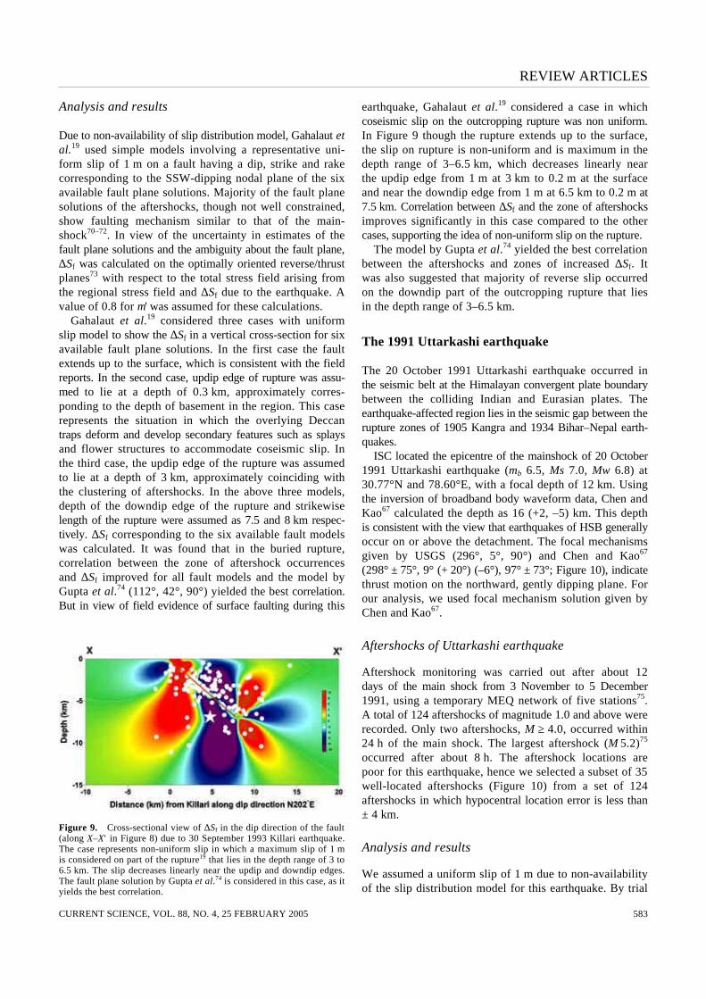
Due to non-availability of slip distribution model, Gahalaut et al.19 used simple models involving a representative uni-form slip of 1 m on a fault having a dip, strike and rake corresponding to the SSW-dipping nodal plane of the six available fault plane solutions. Majority of the fault plane solutions of the aftershocks, though not well constrained, show faulting mechanism similar to that of the main-shock70–72. In view of the uncertainty in estimates of the fault plane solutions and the ambiguity about the fault plane, ∆Sf was calculated on the optimally oriented reverse/thrust planes73 with respect to the total stress field arising from the regional stress field and ∆Sf due to the earthquake. A value of 0.8 for µ' was assumed for these calculations. Gahalaut et al.19 considered three cases with uniform slip model to show the ∆Sf in a vertical cross-section for six available fault plane solutions. In the first case the fault extends up to the surface, which is consistent with the field reports. In the second case, updip edge of rupture was assu-med to lie at a depth of 0.3 km, approximately corres-ponding to the depth of basement in the region. This case represents the situation in which the overlying Deccan traps deform and develop secondary features such as splays and flower structures to accommodate coseismic slip. In the third case, the updip edge of the rupture was assumed to lie at a depth of 3 km, approximately coinciding with the clustering of aftershocks. In the above three models, depth of the downdip edge of the rupture and strikewise length of the rupture were assumed as 7.5 and 8 km respec-tively. ∆Sf corresponding to the six available fault models was calculated. It was found that in the buried rupture, correlation between the zone of aftershock occurrences and ∆Sf improved for all fault models and the model by Gupta et al.74 (112°, 42°, 90°) yielded the best correlation. But in view of field evidence of surface faulting during this

Figure 9. Cross-sectional view of ∆Sf in the dip direction of the fault (along X–X′ in Figure 8) due to 30 September 1993 Killari earthquake. The case represents non-uniform slip in which a maximum slip of 1 m is considered on part of the rupture19 that lies in the depth range of 3 to 6.5 km. The slip decreases linearly near the updip and downdip edges. The fault plane solution by Gupta et al.74 is considered in this case, as it yields the best correlation.

earthquake, Gahalaut et al.19 considered a case in which coseismic slip on the outcropping rupture was non uniform. In Figure 9 though the rupture extends up to the surface, the slip on rupture is non-uniform and is maximum in the depth range of 3–6.5 km, which decreases linearly near the updip edge from 1 m at 3 km to 0.2 m at the surface and near the downdip edge from 1 m at 6.5 km to 0.2 m at 7.5 km. Correlation between ∆Sf and the zone of aftershocks improves significantly in this case compared to the other cases, supporting the idea of non-uniform slip on the rupture. The model by Gupta et al.74 yielded the best correlation between the aftershocks and zones of increased ∆Sf. It was also suggested that majority of reverse slip occurred on the downdip part of the outcropping rupture that lies in the depth range of 3–6.5 km.

The 1991 Uttarkashi earthquake

The 20 October 1991 Uttarkashi earthquake occurred in the seismic belt at the Himalayan convergent plate boundary between the colliding Indian and Eurasian plates. The earthquake-affected region lies in the seismic gap between the rupture zones of 1905 Kangra and 1934 Bihar–Nepal earth-quakes. ISC located the epicentre of the mainshock of 20 October 1991 Uttarkashi earthquake (mb 6.5, Ms 7.0, Mw 6.8) at 30.77°N and 78.60°E, with a focal depth of 12 km. Using the inversion of broadband body waveform data, Chen and Kao67 calculated the depth as 16 (+2, –5) km. This depth is consistent with the view that earthquakes of HSB generally occur on or above the detachment. The focal mechanisms given by USGS (296°, 5°, 90°) and Chen and Kao67 (298° ± 75°, 9° (+ 20°) (–6°), 97° ± 73°; Figure 10), indicate thrust motion on the northward, gently dipping plane. For our analysis, we used focal mechanism solution given by Chen and Kao67.

Aftershocks of Uttarkashi earthquake

Aftershock monitoring was carried out after about 12 days of the main shock from 3 November to 5 December 1991, using a temporary MEQ network of five stations75. A total of 124 aftershocks of magnitude 1.0 and above were recorded. Only two aftershocks, M ≥ 4.0, occurred within 24 h of the main shock. The largest aftershock (M 5.2)75 occurred after about 8 h. The aftershock locations are poor for this earthquake, hence we selected a subset of 35 well-located aftershocks (Figure 10) from a set of 124 aftershocks in which hypocentral location error is less than ± 4 km.


We assumed a uniform slip of 1 m due to non-availability of the slip distribution model for this earthquake. By trial

REVIEW ARTICLES


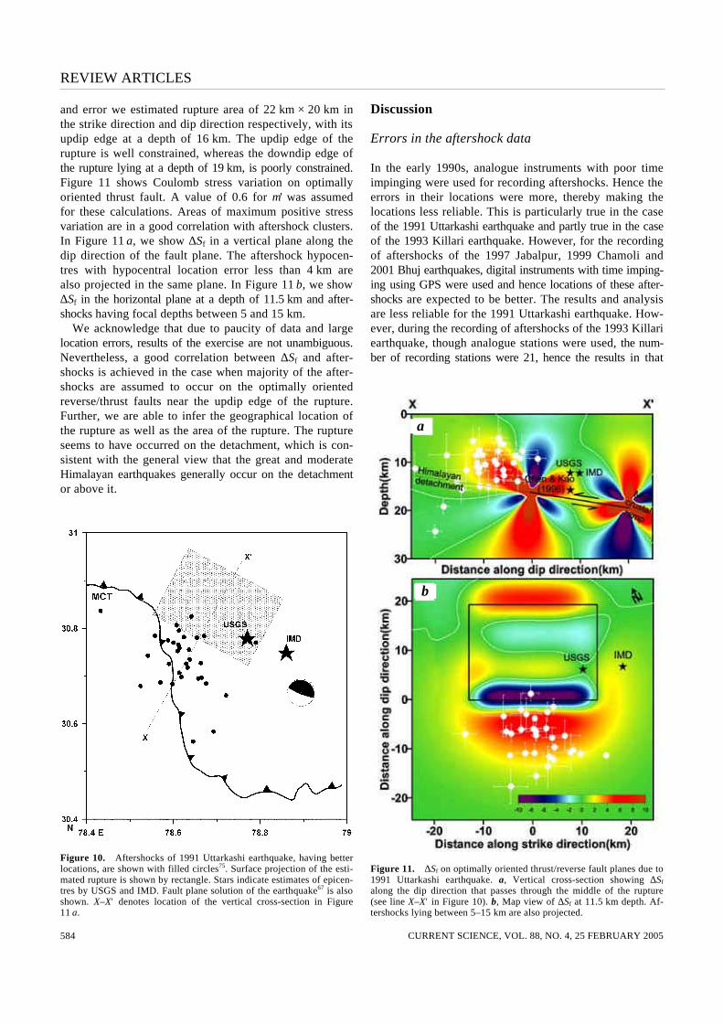
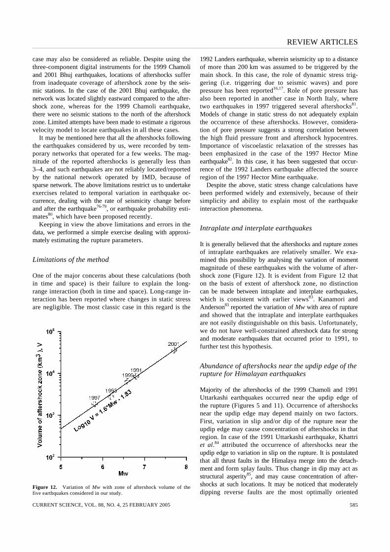
and error we estimated rupture area of 22 km × 20 km in the strike direction and dip direction respectively, with its updip edge at a depth of 16 km. The updip edge of the rupture is well constrained, whereas the downdip edge of the rupture lying at a depth of 19 km, is poorly constrained. Figure 11 shows Coulomb stress variation on optimally oriented thrust fault. A value of 0.6 for µ' was assumed for these calculations. Areas of maximum positive stress variation are in a good correlation with aftershock clusters. In Figure 11 a, we show ∆Sf in a vertical plane along the dip direction of the fault plane. The aftershock hypocen-tres with hypocentral location error less than 4 km are also projected in the same plane. In Figure 11 b, we show ∆Sf in the horizontal plane at a depth of 11.5 km and after-shocks having focal depths between 5 and 15 km. We acknowledge that due to paucity of data and large location errors, results of the exercise are not unambiguous. Nevertheless, a good correlation between ∆Sf and after-shocks is achieved in the case when majority of the after-shocks are assumed to occur on the optimally oriented reverse/thrust faults near the updip edge of the rupture. Further, we are able to infer the geographical location of the rupture as well as the area of the rupture. The rupture seems to have occurred on the detachment, which is con-sistent with the general view that the great and moderate Himalayan earthquakes generally occur on the detachment or above it.

Figure 10. Aftershocks of 1991 Uttarkashi earthquake, having better locations, are shown with filled circles75. Surface projection of the esti-mated rupture is shown by rectangle. Stars indicate estimates of epicen-tres by USGS and IMD. Fault plane solution of the earthquake67 is also shown. X–X′ denotes location of the vertical cross-section in Figure 11 a.

Discussion

Errors in the aftershock data

In the early 1990s, analogue instruments with poor time impinging were used for recording aftershocks. Hence the errors in their locations were more, thereby making the locations less reliable. This is particularly true in the case of the 1991 Uttarkashi earthquake and partly true in the case of the 1993 Killari earthquake. However, for the recording of aftershocks of the 1997 Jabalpur, 1999 Chamoli and 2001 Bhuj earthquakes, digital instruments with time imping-ing using GPS were used and hence locations of these after-shocks are expected to be better. The results and analysis are less reliable for the 1991 Uttarkashi earthquake. How-ever, during the recording of aftershocks of the 1993 Killari earthquake, though analogue stations were used, the num-ber of recording stations were 21, hence the results in that

Figure 11. ∆Sf on optimally oriented thrust/reverse fault planes due to 1991 Uttarkashi earthquake. a, Vertical cross-section showing ∆Sf along the dip direction that passes through the middle of the rupture (see line X–X′ in Figure 10). b, Map view of ∆Sf at 11.5 km depth. Af-tershocks lying between 5–15 km are also projected.

a

b

REVIEW ARTICLES


case may also be considered as reliable. Despite using the three-component digital instruments for the 1999 Chamoli and 2001 Bhuj earthquakes, locations of aftershocks suffer from inadequate coverage of aftershock zone by the seis-mic stations. In the case of the 2001 Bhuj earthquake, the network was located slightly eastward compared to the after-shock zone, whereas for the 1999 Chamoli earthquake, there were no seismic stations to the north of the aftershock zone. Limited attempts have been made to estimate a rigorous velocity model to locate earthquakes in all these cases. It may be mentioned here that all the aftershocks following the earthquakes considered by us, were recorded by tem-porary networks that operated for a few weeks. The mag-nitude of the reported aftershocks is generally less than 3–4, and such earthquakes are not reliably located/reported by the national network operated by IMD, because of sparse network. The above limitations restrict us to undertake exercises related to temporal variation in earthquake oc-currence, dealing with the rate of seismicity change before and after the earthquake76-79, or earthquake probability esti-mates80, which have been proposed recently. Keeping in view the above limitations and errors in the data, we performed a simple exercise dealing with approxi-mately estimating the rupture parameters.

Limitations of the method

One of the major concerns about these calculations (both in time and space) is their failure to explain the long-range interaction (both in time and space). Long-range in-teraction has been reported where changes in static stress are negligible. The most classic case in this regard is the

Figure 12. Variation of Mw with zone of aftershock volume of the five earthquakes considered in our study.

1992 Landers earthquake, wherein seismicity up to a distance of more than 200 km was assumed to be triggered by the main shock. In this case, the role of dynamic stress trig-gering (i.e. triggering due to seismic waves) and pore pressure has been reported16,17. Role of pore pressure has also been reported in another case in North Italy, where two earthquakes in 1997 triggered several aftershocks81. Models of change in static stress do not adequately explain the occurrence of these aftershocks. However, considera-tion of pore pressure suggests a strong correlation between the high fluid pressure front and aftershock hypocentres. Importance of viscoelastic relaxation of the stresses has been emphasized in the case of the 1997 Hector Mine earthquake82. In this case, it has been suggested that occur-rence of the 1992 Landers earthquake affected the source region of the 1997 Hector Mine earthquake. Despite the above, static stress change calculations have been performed widely and extensively, because of their simplicity and ability to explain most of the earthquake interaction phenomena.

Intraplate and interplate earthquakes

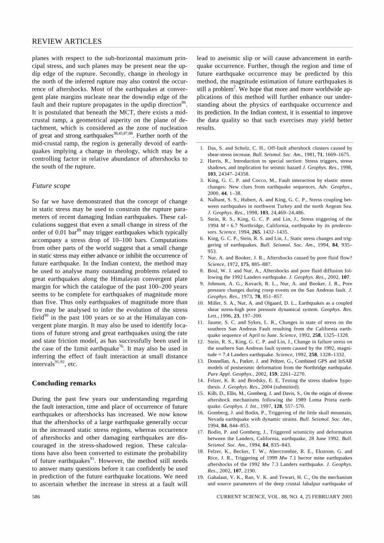
It is generally believed that the aftershocks and rupture zones of intraplate earthquakes are relatively smaller. We exa-mined this possibility by analysing the variation of moment magnitude of these earthquakes with the volume of after-shock zone (Figure 12). It is evident from Figure 12 that on the basis of extent of aftershock zone, no distinction can be made between intraplate and interplate earthquakes, which is consistent with earlier views83. Kanamori and Anderson83 reported the variation of Mw with area of rupture and showed that the intraplate and interplate earthquakes are not easily distinguishable on this basis. Unfortunately, we do not have well-constrained aftershock data for strong and moderate earthquakes that occurred prior to 1991, to further test this hypothesis.

Abundance of aftershocks near the updip edge of the rupture for Himalayan earthquakes

Majority of the aftershocks of the 1999 Chamoli and 1991 Uttarkashi earthquakes occurred near the updip edge of the rupture (Figures 5 and 11). Occurrence of aftershocks near the updip edge may depend mainly on two factors. First, variation in slip and/or dip of the rupture near the updip edge may cause concentration of aftershocks in that region. In case of the 1991 Uttarkashi earthquake, Khattri et al.84 attributed the occurrence of aftershocks near the updip edge to variation in slip on the rupture. It is postulated that all thrust faults in the Himalaya merge into the detach-ment and form splay faults. Thus change in dip may act as structural asperity85, and may cause concentration of after-shocks at such locations. It may be noticed that moderately dipping reverse faults are the most optimally oriented

REVIEW ARTICLES


planes with respect to the sub-horizontal maximum prin-cipal stress, and such planes may be present near the up-dip edge of the rupture. Secondly, change in rheology in the north of the inferred rupture may also control the occur-rence of aftershocks. Most of the earthquakes at conver-gent plate margins nucleate near the downdip edge of the fault and their rupture propagates in the updip direction86. It is postulated that beneath the MCT, there exists a mid-crustal ramp, a geometrical asperity on the plane of de-tachment, which is considered as the zone of nucleation of great and strong earthquakes38,45,87,88. Further north of the mid-crustal ramp, the region is generally devoid of earth-quakes implying a change in rheology, which may be a controlling factor in relative abundance of aftershocks to the south of the rupture.

Future scope

So far we have demonstrated that the concept of change in static stress may be used to constrain the rupture para-meters of recent damaging Indian earthquakes. These cal-culations suggest that even a small change in stress of the order of 0.01 bar89 may trigger earthquakes which typically accompany a stress drop of 10–100 bars. Computations from other parts of the world suggest that a small change in static stress may either advance or inhibit the occurrence of future earthquake. In the Indian context, the method may be used to analyse many outstanding problems related to great earthquakes along the Himalayan convergent plate margin for which the catalogue of the past 100–200 years seems to be complete for earthquakes of magnitude more than five. Thus only earthquakes of magnitude more than five may be analysed to infer the evolution of the stress field90 in the past 100 years or so at the Himalayan con-vergent plate margin. It may also be used to identify loca-tions of future strong and great earthquakes using the rate and state friction model, as has successfully been used in the case of the Izmit earthquake76. It may also be used in inferring the effect of fault interaction at small distance intervals91,92, etc.

Concluding remarks

During the past few years our understanding regarding the fault interaction, time and place of occurrence of future earthquakes or aftershocks has increased. We now know that the aftershocks of a large earthquake generally occur in the increased static stress regions, whereas occurrence of aftershocks and other damaging earthquakes are dis-couraged in the stress-shadowed region. These calcula-tions have also been converted to estimate the probability of future earthquakes91. However, the method still needs to answer many questions before it can confidently be used in prediction of the future earthquake locations. We need to ascertain whether the increase in stress at a fault will

lead to aseismic slip or will cause advancement in earth-quake occurrence. Further, though the region and time of future earthquake occurrence may be predicted by this method, the magnitude estimation of future earthquakes is still a problem2. We hope that more and more worldwide ap-plications of this method will further enhance our under-standing about the physics of earthquake occurrence and its prediction. In the Indian context, it is essential to improve the data quality so that such exercises may yield better results.

1. Das, S. and Scholz, C. H., Off-fault aftershock clusters caused by shear-stress increase. Bull. Seismol. Soc. Am., 1981, 71, 1669–1675.

2. Harris, R., Introduction to special section: Stress triggers, stress shadows, and implication for seismic hazard J. Geophys. Res., 1998, 103, 24347–24358.

3. King, G. C. P. and Cocco, M., Fault interaction by elastic stress changes: New clues from earthquake sequences. Adv. Geophys., 2000, 44, 1–38.

4. Nalbant, S. S., Hubert, A. and King, G. C. P., Stress coupling bet-ween earthquakes in northwest Turkey and the north Aegean Sea. J. Geophys. Res., 1998, 103, 24,469–24,486.

5. Stein, R. S., King, G. C. P. and Lin, J., Stress triggering of the 1994 M = 6.7 Northridge, California, earthquake by its predeces-sors. Science, 1994, 265, 1432–1435.

6. King, G. C. P., Stein, R. S. and Lin, J., Static stress changes and trig-gering of earthquakes. Bull. Seismol. Soc. Am., 1994, 84, 935– 953.

7. Nur, A. and Booker, J. R., Aftershocks caused by pore fluid flow? Science, 1972, 175, 885–887.

8. Bosl, W. J. and Nur, A., Aftershocks and pore fluid diffusion fol-lowing the 1992 Landers earthquake. J. Geophys. Res., 2002, 107.

9. Johnson, A. G., Kovach, R. L., Nur, A. and Booker, J. R., Pore pressure changes during creep events on the San Andreas fault. J. Geophys. Res., 1973, 78, 851–857.

10. Miller, S. A., Nur, A. and Olgaard, D. L., Earthquakes as a coupled shear stress-high pore pressure dynamical system. Geophys. Res. Lett., 1996, 23, 197–200.

11. Jaume, S. C. and Sykes, L. R., Changes in state of stress on the southern San Andreas Fault resulting from the California earth-quake sequence of April to June. Science, 1992, 258, 1325–1328.

12. Stein, R. S., King, G. C. P. and Lin, J., Change in failure stress on the southern San Andreas fault system caused by the 1992, magni-tude = 7.4 Landers earthquake. Science, 1992, 258, 1328–1332.

13. Donnellan, A., Parker, J. and Peltzer, G., Combined GPS and InSAR models of postseismic deformation from the Northridge earthquake. Pure Appl. Geophys., 2002, 159, 2261–2270.

14. Felzer, K. R. and Brodsky, E. E, Testing the stress shadow hypo-thesis. J. Geophys. Res., 2004 (submitted).

15. Kilb, D., Ellis, M., Gomberg, J. and Davis, S., On the origin of diverse aftershock mechanisms following the 1989 Loma Prieta earth-quake. Geophys. J. Int., 1997, 128, 557–570.

16. Gomberg, J. and Bodin, P., Triggering of the little skull mountain, Nevada earthquake with dynamic strains. Bull. Seismol. Soc. Am., 1994, 84, 844–853.

17. Bodin, P. and Gomberg, J., Triggered seismicity and deformation between the Landers, California, earthquake, 28 June 1992. Bull. Seismol. Soc. Am., 1994, 84, 835–843.

18. Felzer, K., Becker, T. W., Abercrombie, R. E., Ekstrom, G. and Rice, J. R., Triggering of 1999 Mw 7.1 hector mine earthquakes aftershocks of the 1992 Mw 7.3 Landers earthquake. J. Geophys. Res., 2002, 107, 2190.

19. Gahalaut, V. K., Rao, V. K. and Tewari, H. C., On the mechanism and source parameters of the deep crustal Jabalpur earthquake of

REVIEW ARTICLES


21 May 1997: Constraints from aftershocks and change in static stress. Geophys. J. Int., 2004, 156, 345–351.

20. Gahalaut, V. K., Kalpna and Raju, P. S., Rupture mechanism of the 1993 Killari earthquake, India: Constraint from aftershocks and static stress change. Tectonophysics, 2003, 369, 71–78.

21. Toda, S. and Stein, R. S., Did stress triggering cause the large off-fault aftershocks of the 25 March 1998 Mw = 8.1 Antarctic plate earthquake? Geophys. Res. Lett., 2000, 27, 2301–2304.

22. Gowd, T. N., Rao, S. V. S. and Gaur, V. K., Tectonic stress field in the Indian subcontinent. J. Geophys. Res., 1992, 97, 11879–11888.

23. Bilham, R. and Gaur, V. K., Geodetic contributions to the study of seismotectonicsof India. Curr. Sci., 2000, 79, 1259–1269.

24. Biswas, S. K., Regional tectonic framework, structure and evolu-tion of the western marginal basins of India. Tectonophysics, 1987, 135, 302–327.

25. Merh, S. S., Geology of Gujarat, Geological Society of India, 1995, p. 222.

26. Hengesh, J. V. and Lettis, W. R., Geologic and tectonic setting. In Bhuj, India Earthquake of 26 January 2001 Reconnaissance Report (eds Jain, S. K. et al.), Earthquake Spectra, 2002, vol. 18A, pp. 7–22.

27. Talwani, P. and Gangopadhyay, A., Tectonic framework of the Kachchh earthquake of 26 January. Seismol. Res. Lett., 2001, 72, 336–345.

28. Malik, J. N., Sohoni, P. S., Merh, S. S. and Karanth, R. V., Palaeo-seismology and neotectonism of Kachchh western India. In Active Fault Research for the New Millennium, Proceedings of the Hokudan International Symposium and School of Active Faulting, 2000, pp. 251–259.

29. Bilham, R., Slip parameters for the Rann of Kachchh, India, 16 June 1819, earthquake, quantified from contemporary accounts. In Coastal Tectonics (eds Stewart, I. S. and Vita-Finzi, C., Geological Society London, Special Publications, London, UK, 1998, vol. 146, pp. 295–319.

30. Rajendran, C. P. and Rajendran, K., Characteristics of deformation and past seismicity associated with the 1819 Kutch earthquake, Northwestern India. Bull. Seismol. Soc. Am., 2001, 91, 407–426.

31. Chung, W. Y. and Gao, H., Source parameters of the Anjar earth-quake of 21 July 1956, India and its seismotectonics implications for the Kutch rift basins. Tectonophysics, 1995, 242, 281–292.

32. Wesnousky, S. G. et al., Eight days in Bhuj: Field report bearing on surface rupture and genesis of the 26 January 2001 Republic Day earthquake of India. Seismol. Res. Lett., 2001, 72, 514–524.

33. Antolik, M. and Dreger, D. S., Rupture process of the 26 January 2001 Mw 7.6 Bhuj, India, earthquake from teleseismic broadband data. Bull. Seismol. Soc. Am., 2003, 93, 1235–1248.

34. Negishi, H. et al., Size and orientation of the fault plane for the 2001 Gujarat, India earthquake (Mw 7.7) from aftershock observa-tions: A high stress drop event. Geophys. Res. Lett., 2002, 29, 10–14.

35. Engdahl, E. R., Dewey, J. W. and Fujita, K., Earthquake location in island arcs. Phys. Earth Planet. Inter., 1982, 30, 145–156.

36. Gahalaut, V. K. and Bürgmann, R., Constraints on the source para-meters of the 26 January 2001 Bhuj, India earthquake from satellite images. Bull. Seismol. Soc. Am., 2004, 94, 2407–2413.

37. Mandal, P. et al., Characterization of the causative fault system for the 2001 Bhuj earthquake of Mw 7.7. Tectonophysics, 2004, 378, 105–121.

38. Seeber, L. and Armbruster, J. G., Great detachment earthquakes along the Himalayan arc and long term forecasting. In Earthquake Prediction – An International Review, Maurice Ewing Series, American Geophysical Union, Washington DC, 1981, pp. 259–277.

39. Ni, J. and Barazangi, M., Seismotectonics of the Himalaya collision zone: Geometry of the underthrusting Indian plate beneath the Himalaya. J. Geophys. Res., 1984, 89, 1147–1164.

40. Molnar, P., A review of the seismicity and the rates of active un-derthrusting and deformation at the Himalaya. J. Himalayan Geol., 1990, 1, 131–154.

41. Cattin, R. and Avouac, J. P., Modeling mountain building and the seismic cycle in the Himalaya of Nepal. J. Geophys. Res., 2000, 105, 13,389–13,407.

42. Bilham, R., Larson, K., Freymuller, J. and Project Idylhim mem-bers, GPS measurements of present-day convergence across the Nepal Himalaya. Nature, 1997, 386, 61–64.

43. Gahalaut, V. K. and Chander, R., On interseismic elevation changes and strain accumulation for great thrust earthquakes in the Nepal Himalaya. Geophys. Res. Lett., 1997, 24, 1011–1014.

44. Gahalaut, V. K. and Chander, R., On interseismic elevation changes observed near 75.5°E longitude in the NW Himalaya. Bull. Seis-mol. Soc. Am., 1999, 89, 3, 837–843.

45. Gahalaut, V. K. and Kalpna, Himalayan mid-crustal ramp. Curr. Sci., 2001, 81, 1641–1646.

46. IMD, Chamoli earthquake of 29 March 1999 and its aftershocks: A consolidated document. Meteorol. Monogr. Seismol., 2000, 2/2000, 70.

47. Mandal, P., Rastogi, B. K. and Gupta, H. K., Recent Indian earth-quakes. Curr. Sci., 2000, 79, 1334–1346.

48. Kayal, J. R., Ram, S., Singh, O. P., Chakraborty, P. K. and Karu-nakar, G., Aftershocks of the March 1999 Chamoli earthquake and seismotectonics structure of the Garhwal Himalaya. Bull. Seismol. Soc. Am., 2003, 93, 109–117.

49. Anderson, G. and Johnson, H., A new statistical test for static stress triggering: Application to the 1987 superstition hills earth-quake sequence. J. Geophys. Res., 1999, 104, 20153–20168.

50. Chander, R. and Sharma, R., Could the main Chamoli earthquake of 1999 have triggered some of the aftershocks? Himalayan Geol., 2002, 23, 39–43.

51. Liu, L. and Zoback, M. D., Lithosphere strength and intraplate sei-smicity in the New Madrid seismic zone. Tectonics, 1997, 16, 585–595.

52. Fermor, L. L., An attempt at the correlation of the ancient schis-tose formation of peninsular India. Mem. Geol. Surv. India, 1936, 70, 217.

53. Nair, K. K. K., Jain, S. C. and Yedekar, D. B., Geology, structure and tectonics of the Son–Narmada–Tapti lineament zone. Rec. Geol. Surv. India, 1985, 117, 138–147.

54. Roy, A. and Bandyopadhyay, B. K., Tectonic and structural pattern of the Mahakoshal belt of central India. A discussion. Workshop on Precambrian of central India. Geol. Surv. India, Spl. Pap. 28, 1990, pp. 226–240.

55. GSI report, Geoscientific studies of the Son–Narmada–Tapti lineament zone. Geol. Surv. India, 1995, 10, 371.

56. Acharya, S. K., Kayal, J. R., Roy, A. and Chaturvedi, R. K., Jabal-pur earthquake of 22 May 1997: Constraint from aftershock study. J. Geol. Soc. India, 1998, 51, 295–304.

57. Gupta, H. K., Indramohan and Hari Narain, The Broach earthquake of 23 March 1970. Bull. Seismol. Soc. Am., 1972, 62, 47–61.

58. Rao, B. R. and Rao, P. S., Historical seismicity of peninsular India. Bull. Seismol. Soc. Am., 1984, 74, 2519–2533.

59. Johnston, A. C. et al., The earthquakes of stable continental regions: Assessment of large earthquake potential. EPRI TR-102261 (ed. Schneider, J. F.), Electric Power Research Institute, Palo Alto, 1994, p. 309.

60. Bhattacharya, S. N., Ghosh, A. K., Suresh, G., Baidya, P. R. and Saxena, R. C., Source parameters of Jabalpur earthquake of 22 May 1997. Curr. Sci., 1997, 73, 855–863.

61. Rajendran, K. and Rajendran, C. P., Characteristics of the 1997 Jabalpur earthquake and their bearing on its mechanism. Curr. Sci., 1998, 74, 168–174.

62. Ramesh, D. S. and Estabrook, C. H., Rupture histories of two stable continental region earthquakes of India. Proc. Indian Acad. Sci. (Earth Planet. Sci.), 1998, 107, L225–L233.

63. Kayal, J. R., Seismotectonic study of the two recent SCR earth-quakes in central India. J. Geol. Soc. India, 2000, 55, 123–138.

64. Singh, S. K. et al.,Crustal and upper mantle structure of peninsular India and source parameters of the 21 May 1997 Jabalpur earth-

REVIEW ARTICLES


quake (Mw = 5.8): Results from a new regional broadband net-work. Bull. Seismol. Soc. Am., 1999, 89, 1631–1641.

65. Rao, N. P., Tsukuda, T., Koruga, M., Bhatia, S. C. and Suresh, G., Deep lower crustal earthquakes in central India: Inferences from analysis of regional broadband data of the 1997 May 21 Jabalpur earthquake. Geophys. J. Int., 2002, 148, 132–138.

66. Seeber, L. et al., The 1993 Killari earthquake in central India: A new fault in Mesozoic flows? J. Geophys. Res., 1996, 101, 8543–8560.

67. Chen, W. P. and Kao, H., Seismotectonics of Asia: Some recent progress. In The Tectonic Evolution of Asia (eds Yin, A. and Har-rison, T. M.), Cambridge Univ. Press, New York, 1996, pp. 37–62.

68. Baumbach, M. et al., Study of the foreshocks and aftershocks of the intraplate Latur earthquake of 30 September 1993, India. Mem. Geol. Soc. India, 1996, 35, 33–63.

69. Gupta, H. K. et al., An investigation into the Latur earthquake of 29 September 1993 in southern India. Tectonophysics, 1998, 287, 299–318.

70. Anon, Latur earthquake of 30 September 1993 and its aftershocks. A consolidated Report. India Meteorological Department, New Delhi, 1994, pp. 1–37.

71. Rao, C. V. R. and Raju, P. S., Study of the aftershock activity and source parameters of the Latur earthquake of 30 September 1993. J. Geol. Soc. India, 1996, 47, 243–250.

72. Rao, N. P., Analysis of aftershock data of the Latur (Mb 6.3) earthquake using the seismic analysis software (SEISAN). Techni-cal Report No. 98-01, Institute of Solid Earth Physics, University of Bergen, Norway, 1998.

73. Anderson, G. and Johnson, H., A new statistical test for static stress triggering: Application to the 1987 Superstition Hills earth-quake sequence. J. Geophys. Res., 1999, 104, 20153–20168.

74. Gupta, H. K., Rastogi, B. K., Mohan, I., Rao, C. V. R. K., Sarma, S. V. S. and Rao, R. U. M., An investigation into the Latur earth-quake of 29 September, in southern India. Tectonophysics, 1998, 287, 299–318.

75. Kayal, J. R., Precursor seismicity, foreshocks and aftershocks of the Uttarkashi earthquake of 20 October 1991 at Garhwal Himalaya. Tectonophysics, 1996, 263, 339–345.

76. Stein, R. S., Barka, A. A. and Dieterich, J. H., Progressive failure on the North Anatolian fault since 1939 by earthquake stress trig-gering. Geophys. J. Int., 1997, 128, 594–604.

77. Toda, S., Stein, R. S., Reasenberg, P. A., Dieterich, J. H. and Yo-shida, A., Stress transfers by the 1995 Mw = 6.9 Kobe, Japan, shock: Effect on aftershocks and future earthquake probabilities. J. Geophys. Res., 1998, 103, 24543–24566.

78. Parsons, T., Toda, S., Stein, R. S., Barka, A. and Dieterich, J. H., Heightened odds of large earthquakes near Istanbul: An interac-tion-based probability calculation. Science, 2000, 288, 661–665.

79. Toda, S. and Stein, R. S., Response of the San Andreas Fault to the 1983 Coalinga-Nuñez Earthquakes: An application of interac-tion-based probabilities for Parkfield. J. Geophys. Res., 2002, 107, 2126.

80. Hardebeck, J. L., Stress triggering and earthquake probability es-timates. J. Geophys. Res., 2004, 109, B04310

81. Miller, S. A. et al., Aftershocks driven by a high-pressure CO2 source at depth. Nature, 2004, 427, 724–727.

82. Freed, A. M. and Lin, J., Time dependent changes in failure stress following thrust earthquakes. J. Geophys. Res., 1998, 103, 24,393–24,409.

83. Kanamori, H. and Anderson, D. L., Theoretical basis of some em-pirical relations in seismology. Bull. Seismol. Soc. Am., 1975, 65, 1073–1095.

84. Khattri, K. N., Zeng, Y., Anderson, J. G. and Brune, J., Inversion of strong motion waveforms for source slip function of 1991 Uttar-kashi earthquake, Himalaya. J. Himalayan Geol., 1994, 5, 163–192.

85. Lay, T. and Wallace, T. C., Modern Global Seismology, Academic Press, New York, 1995, p. 517.

86. Kelleher, J. A., Rupture zones of large South American earthquakes and some predictions. J. Geophys. Res., 1972, 77, 2087–2103.

87. Pandey, M. R., Tandukar, R. P., Avouac, J. P., Lave, J. and Massot, J. P., Interseismic strain accumulation on the Himalayan crustal ramp (Nepal). Geophys. Res. Lett., 1995, 22, 751–754.

88. Kayal, J. R., Microearthquake activity in some parts of the Hima-laya and the tectonic model. Tectonophysics, 2001, 339, 331–351.

89. Reasenberg, P. A. and Simpson, R. W., Response of regional sei-smicity to the static stress change produced by the Loma Prieta earthquake. Science, 1992, 255, 1687–1690.

90. Deng, J. and Sykes, L. R., Evolution of stress field in southern Cali-fornia and triggering of moderate-size earthquakes: A 200 years perspective. J. Geophys. Res., 1997, 102, 9859–9886.

91. Stein, R. S., The role of stress transfer in earthquake occurrence. Nature, 1999, 402, 605–609.

92. Gahalaut, V. K., Kalpna and Singh, S. K., Fault interaction and earthquake triggering in the Koyna–Warna region, India. Geophys. Res. Lett., 2004, 31, L11614.

ACKNOWLEDGEMENTS. We thank three anonymous reviewers for their comments on the article. We thank the Director, NGRI, Hyderabad for support and permission to publish this article. Financial support from CSIR, New Delhi and support from Dr R. K. Chadha are acknowledged. Received 15 August 2004; revised accepted 11 October 2004

Coulomb stress changes and aftershocks of recent Indian earthquakes

Documents