cost1401.doc

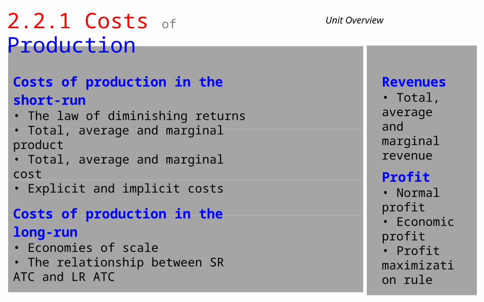
2.2.1 Costs of Production Unit Overview

Costs of production in the short-run• The law of diminishing returns• Total, average and marginal product• Total, average and marginal cost• Explicit and implicit costs

Costs of production in the long-run• Economies of scale• The relationship between SR ATC and LR ATC

Revenues• Total, average and marginal revenue

Profit• Normal profit• Economic profit• Profit maximization rule

Costs of Production

Cost s of producti onCost- min imizationProfi t maxi mizat ionLaw of di mini shingret urnsEconomies of scal e

Co s t s of P r oduct i on

P r act i ce A c t i vi t ies

Theory of t he Firm Gl ossar y

2.2.1 Costs of ProductionIntroduction to Costs of Production

Introduction to Costs ofProduction

Firms in a market economy are the provides of the goods and services that households demand in the product market. The incentive that drives firms to provide households with products is that of Profit maximization: The goal of most firms is to maximize their profits. To do so, they must produce at a level of output at which the difference between their revenues and their costsis max

To determine whether it will earn a profit at a particular level of output, a firm must,

therefore,

consider two economic variables: its costs and its revenuesEconomic Costs: These are the explicit money payments a firm makes to resources owners for the use of land, labor and capital:• Includes variable costs (payments for those resources which vary with the level of output)• And fixed costs (payments for those resources which do not vary in quantity with the level of output),• As well as the opportunity cost of the business owner;Economic Revenues: This is the money income a firm earns from the sale of its products to households. At aparticular level of output, a firm’s total revenue equals the price of its product times the quantity sold.

2.2.1 Costs of Production Costs of Production

Short-run versus Long-run Costs of ProductionWhen examining a firm’s costs, we must consider two periods of time.• The short-run: The period of time in which firms can vary only the amount of labor and the

raw materials it uses in its production. Capital and land resources are fixed, and cannot bevaried. Example: When the demand for American automobiles fell in the late 2000s, Ford andGeneral Motors responded in the short-run by reducing the size of their workforces.

• The long-run: The period of time over which firms can vary the quantities of all resourcesthey use in production. The quantities of labor, capital and land resources can all be varied inthe long-run. Example: When demand for American automobiles remained week for overtwo years, Ford and General Motors began closing factories and selling off their capitalequipment to foreign car manufacturers.

Variable costs and fixed costs: A firm’s variable costs are those which change in the short-run as the firm changes its level of output. Fixed costs, on the other hand, remain constant as output varies in the short-run.

In the long-run, all costs are variable, since all resources can be varied…

2.2.1 Costs of Production Short-run Costs of Production

Determining Short-run Costs of ProductionThe primary determinant of a firm’s short-run production costs is the productivity of its short-run variable resources (primarily the labor the firm employs).Productivity: The output produced per unit of input• The greater the average product of variable resources, the lower the average costs of

production in the short-run• The lower the productivity of the variable resource, the higher the average costs of

production• Since in the short-run, only labor and raw materials can be varied in quantity, LABOR IS THE

PRIMARY VARIABLE RESOURCE…Labor productivity in the short-run: As different amounts of labor are added to a fixed amountof capital, the productivity of labor will vary based on the law of diminishing returns, whichstates…

The Law of Diminishing Returns: As more and more of a variable resource (usually labor) is added to fixed resources (capital and land) towards production, the marginal product of the variable resource will increase until a certain point, beyond which marginal product declines.


2.2.1 Costs of ProductionProductivity in the Short-run

Short-run Costs of Production

The productivity of labor is the primary determinant of a firm’s short-run production costs. The table below presents some of the key measures of productivity we must consider when determining short-run costs.

Productivity: The amount of output attributable to a unit of input.

Examples of productivity:

"Better training has increased the productivity of workers" "The new robot is more productive than older versions"

"Adding fertilizer has increased the productivity of farmland"

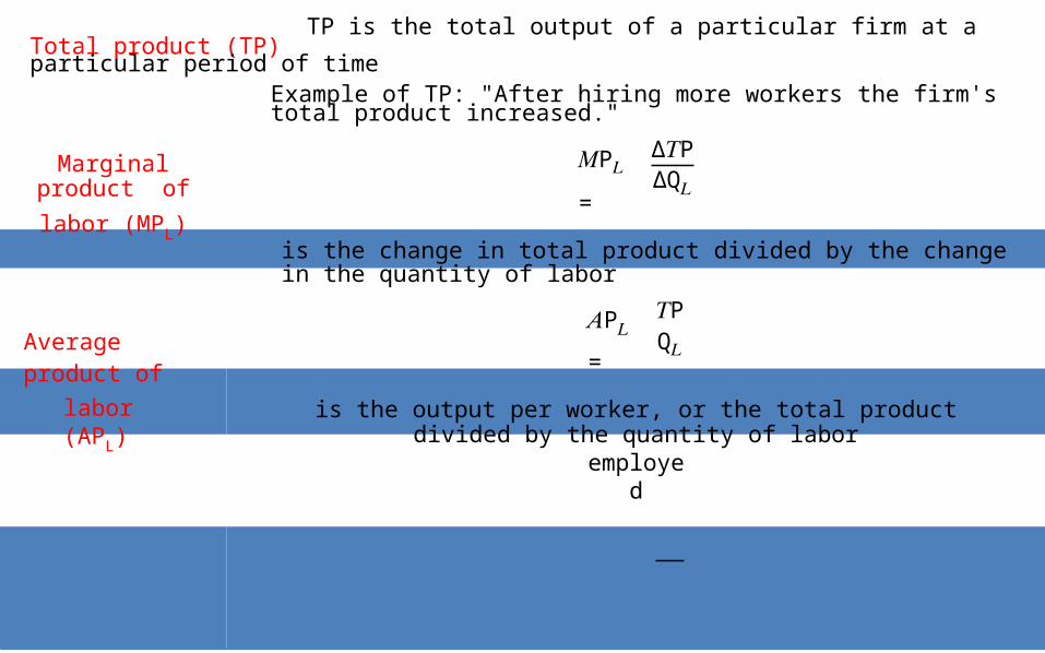
Total product (TP)TP is the total output of a particular firm at a particular period of time

Example of TP: "After hiring more workers the firm's total product increased."∆𝑇PMarginal product of

labor (MPL)

𝑀P𝐿 = ∆Q𝐿is the change in total product divided by the change in the quantity of labor𝑇P

Aver age product of

𝐴P𝐿 = Q𝐿labor (APL) is the output per worker, or the total product divided by the quantity of labor

employed

Quantity of labor (QL)

TotalProduct

MarginalProduct

AverageProduct

0 0 - -

1 4 4 4

2 9 5 4.5

3 15 6 5

4 20 5 5

5 24 4 4.8

6 26 2 4.33

7 26 0 3.7

8 24 -2 3



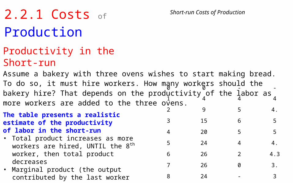
Assume a bakery with three ovens wishes to start making bread. To do so, it must hire workers. How many workers should the bakery hire? That depends on the productivity of the labor as more workers are added to the three ovens.

The table presents a realistic estimate of the productivity of labor in the short-run• Total product increases as more workers are

hired, UNTIL the 8th worker, then total product decreases

• Marginal product (the output contributed by the last worker hired) increases until the 4th worker, and then marginal product begins decreasing.

• Average product (the output per worker) increases until the marginal product becomes lower than AP (at the 5th worker) and then begins decreasing.

• The productivity of labor is at its greatest at around3 or 4 workers, which means the bakery’s average costs will be minimized when employing

approximately 4 workers.



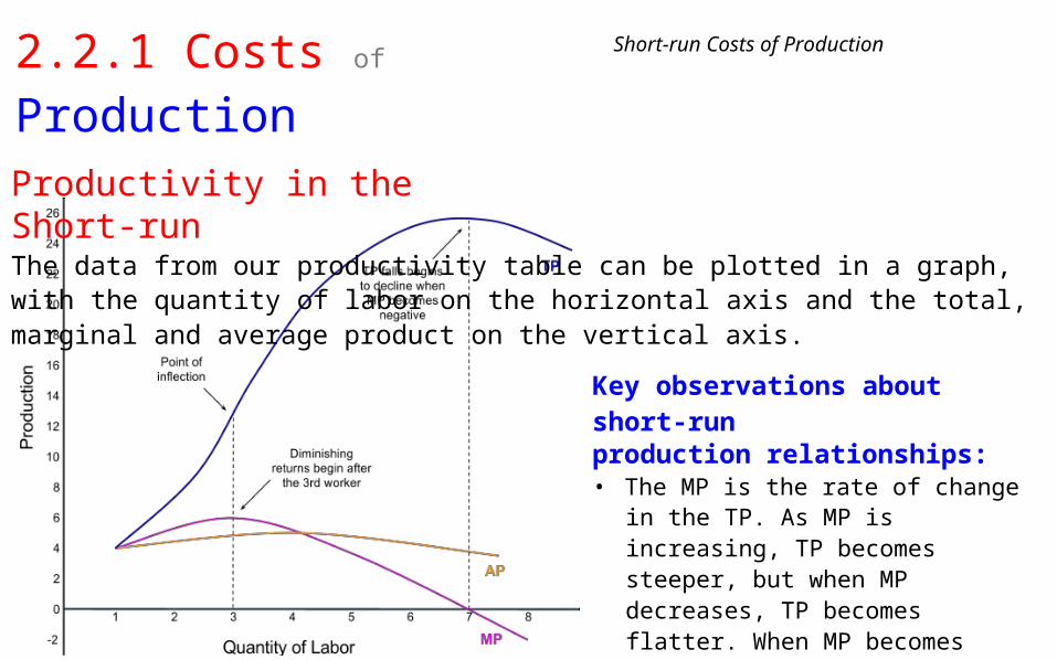
The data from our productivity table can be plotted in a graph, with the quantity of labor on the horizontal axis and the total, marginal and average product on the vertical axis.

Key observations about short-runproduction relationships:• The MP is the rate of change in the TP. As

MP is increasing, TP becomes steeper, but when MP decreases, TP becomes flatter. When MP becomes negative, TP beginsdecreasing.

• MP intersects AP at its highest point.Whenever MP>AP, AP is increasing, butwhen MP<AP, AP is decreasing.

• The bakery begins experiencing diminishingmarginal returns (the output of additionalworkers begins decreasing) after the thirdworker

e

t



If we look more closely at just the marginal product and average product curves, we can learn more about the relationship between these two production variables.Explanation for diminishing returns:• With only three ovens in the bakery, the output

attributable to the 4th – 8th worker becomes less and less.

• This is because there is not enough capital to allowadditional workers to continue to be more and morproductive!

• Up to the 5th worker, adding additional workerscaused the average product to rise, since themarginal product was greater than the average.

• But beyond the 5th worker, diminishing returns wascausing marginal product to fall at such a rate that itwas pulling average output down with it. Workerproductivity declines rapidly after four workers.

• A bakery wanting to minimize costs will not hiremore than four workers.


UN D E R S T AN D ING THE R EL A TI O NS H IPS

BETWE E N T O T A L , MA R G INAL AND A VER A G E P R ODU C T

2.2.1 Costs of ProductionTotal Costs in the Short-run


A firm’s costs in the short-run can be either fixed or variable. The table below presents some of the primary costs a firm faces, and indicates whether they are fixed costs or variable costs.

Resource costs in the short-run

Rent - the payment for land: Rent is fixed in the short-run since firms cannot add this resource toproduction. Rents must be paid regardless of the level of the firm's output.

Interest - the payment for capital: Interest is fixed in the short-run since firms cannot add this resourceFixed Costs inthe short-run

Variable Costs in the short-

run

to production. Interest must be paid on loans regardless of the level of the firm's output.

Normal profit - the minimum level of profit needed just to keep an entrepreneur operating in his current market. If he does not earn normal profit, an entrepreneur will direct his skills towards another market. Normal profit is a cost because if a firm does not earn normal profit, it is not covering its costs and may shut down.

Wages - the payment for labor: Wages are variable in the short-run, since firms can hire or fire workers to use existing land and capital resources. Wage costs increase when new workers are hired, and decrease when workers are laid off.

Transportation costs: Firms pay lower transport costs at lower levels of output.

Raw material costs: vary with the level of output

Manufactured inputs: fewer parts are needed from suppliers when a firm lowers output.



A firm’s total costs include the costs of labor (variable costs) and the costs of capital and landresources (fixed costs).

Total Costs in the Short-run

Total fixed costs (TFC): These are the costs a firm faces that do not vary with changes in short-run output. Could include rent on factory space, interest on capital (already acquired).

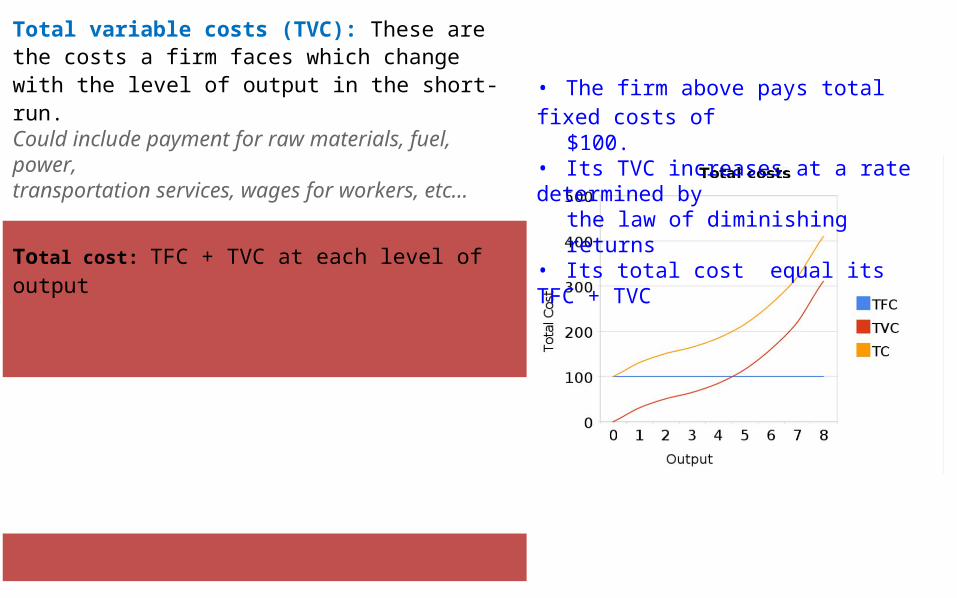
Total variable costs (TVC): These are the costs a firm faces which change with the level of output in the short-run.Could include payment for raw materials, fuel, power,transportation services, wages for workers, etc…

Total cost: TFC + TVC at each level of output

• The firm above pays total fixed costs of$100.

• Its TVC increases at a rate determined bythe law of diminishing returns

• Its total cost equal its TFC + TVC



A firm’s total costs include the costs of labor (variable costs) and the costs of capital and landresources (fixed costs).• TFC: Notice that regardless of the level of output,

TFC remains constant. This is because these are coststhat do not vary with output.

• TVC: Notice that when output is zero, TVC is zero,because you do not need to hire any workers or useany raw materials if you're not producing anything.As output increases, TVC continues to increase

• TC: Notice that when output is zero, TC = TFC. Butonce the factory begins pumping out products, TCrises with TVC. TC is the sum of TFC and TVC, sinceboth fixed and variable costs make up total cost.

Diminishing Returns and the short-run costs of production:• Notice that TC and TVC increase at a decreasing rate at first. This is when marginal product is increasing as more

labor is employed (firms get "more for their money")• However, beyond some point, costs begin to increase at an increasing rate. This is where diminishing returns set

in and MP is decreasing. The firm is getting less additional output from each worker hired, but must pay thesame wages regardless. (The firm gets "less for its money")

2.2.1 Costs of ProductionPer-unit Costs in the Short-run


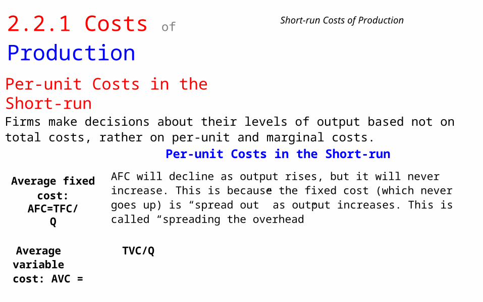
Firms make decisions about their levels of output based not on total costs, rather on per-unit and marginal costs.

Average fixed cost:AFC=TFC/Q

Per-unit Costs in the Short-run

AFC will decline as output rises, but it will never increase. This is because the fixed cost (which never goes up) is “spread out” as output increases. This is called “spreading the overhead”

Average variable cost: AVC = TVC/Q

For simplicity, we will assume that labor is the only variable input, the labor cost per unit of output is the AVC

Average total cost:ATC = TC/Q

Sometimes called unit cost or per unit cost. ATC also equals AFC + AVC

Marginal Cost: MC =∆TVC/∆Q

The additional cost of producing one more unit of output.


From Short-run Productivity to Short-run CostsAs worker productivity increases, firms get "more for their money", meaning per-unit andmarginal cost decrease. When productivity decreases, costs increase.

The relationship between productivity and costs

When productivity of its workers is rising, a firm’s per unit costs are falling, since they're getting more output for each dollar spent on worker wages.

When marginal product is increasing (increasing returns) marginal costis falling. When average product is rising, average variable cost is falling.

When MP and AP are maximimized, MC and AVC are minimized

When workers begin experiencing diminishing returns, MP falls andMC begins to rise.

MP intersects average product at its highest point, and MC intersects average variable cost at its lowest point


SHO R T - R UN P R ODU C TIVIT Y , C O ST S AND THE

L A W OF DIMINIS H ING MA R G INAL R E T URNS

2.2.1 Costs of ProductionGraphing Per-unit Costs in the Short-run


The relationships between a firm’s short-run per unit costs are dictated by the law of diminishing marginal returns

Short-run Cost Relationships

ATC=AFC +AVC

MC andATC/AVC

MC and diminishing

returns

The vertical distance between ATCand AVC equals the AFC at eachlevel of output.

MC intersects both AVC and ATC at their minimum. This is because if the last unit produced cost less than the average, then the average must be falling, and vis versa (just like your test scores!)

MC is at its minimum when MP is at its maximum, because beyond that point diminishing returns sets inand the firm starts getting less for its money!


THE R E L A T I O NSHIPS BE T WE E N SHO R T - R UN

COSTS OF PRODUC TION

2.2.1 Costs of ProductionCosts of Production in the Long-run

Long-run Costs of Production

Long-run is the variable plant period, meaning that firms can open up new plants, add capital to existing plants, or close plans and remove capital if need be.• Because capital and land are variable in the long-run, the law of diminishing returns no longer applies.• A firm’s long-run average costs depend on how productivity of land, labor and capital change as a firm’s

output increases in the variable plant-period.• As a firm’s output increases in the long-run, the firm’s ATC will initially decrease, but eventually increase,

based on the following concepts…

Three ranges of a firm’s long-run Average Total Cost curve

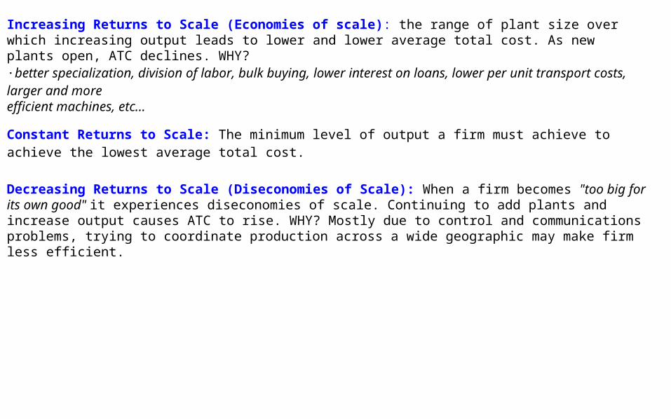
Increasing Returns to Scale (Economies of scale): the range of plant size over which increasing output leads to lower and lower average total cost. As new plants open, ATC declines. WHY?·better specialization, division of labor, bulk buying, lower interest on loans, lower per unit transport costs, larger and moreefficient machines, etc...

Constant Returns to Scale: The minimum level of output a firm must achieve to achieve the lowest average total cost.

Decreasing Returns to Scale (Diseconomies of Scale): When a firm becomes "too big for its own good" it experiences diseconomies of scale. Continuing to add plants and increase output causes ATC to rise. WHY? Mostly due to control

and communications problems, trying to coordinate production across a wide geographic may make firm less efficient.

2.2.1 Costs of ProductionCosts of Production in the Long-run

Long-run Costs of Production

The concept of economies of scale explain why a firm adding new plants and capital equipment to its production will become more efficient as it expands: Examine the long-run average total cost curve below (the orange line)• The blue lines represent the short-run ATC

curves experienced as the firm opens severalfactories in the long-run (from 1 to 7factories).

• As the firm opens its first 4 factories, its ATCcontinuously decreases. The firm isbecoming more efficient in its production.

• With the 5th factory, the firm is no longerexperiencing increasing returns, and insteadhas experienced constant returns to scale.

• With the 6th and 7th factories, the firm’s ATC

is rising, indicating it is becoming lessefficient. The firm is experiencing decreasingreturns to scale.

As a firm increases its output in the long-run (the variable plant period), it at first becomes more and more

efficient, but eventually inefficiencies cause its ATC to rise as the firm gets “too big for its own good”

2.2.1 Costs of Production Long-run Costs of Production

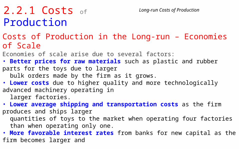
Costs of Production in the Long-run – Economies of ScaleEconomies of scale arise due to several factors:• Better prices for raw materials such as plastic and rubber parts for the toys due to larger

bulk orders made by the firm as it grows.• Lower costs due to higher quality and more technologically advanced machinery operating in

larger factories.• Lower average shipping and transportation costs as the firm produces and ships larger

quantities of toys to the market when operating four factories than when operating only one.• More favorable interest rates from banks for new capital as the firm becomes larger and

therefore more "credit worthy".• More bargaining power with labor unions for lower wages as the firm employers larger

numbers of factory workers.• Improved manufacturing techniques and more highly specialized labor, capital and

managerial expertise.Diseconomies of scale: When a firm becomes to big to manage efficiently, it becomes lessefficient and average costs rise, making the firm less and less competitive. The best thing a firmexperiencing diseconomies of scale can do is reduce its size or break into smaller firms.

2.2.1 Costs of Production Long-run Costs of Production

L ONG- R UN A VER A G E T O T AL C O S T

AND E C ON O MI E S OF SCA L E

2.2.1 Costs of ProductionRevenues

Revenues

Costs are only half the calculation a firm must make when determining its level of economic profits. A firm must also consider its revenues.

Revenues are the income the firm earns from the sale of its good.• Total Revenue = the price the good is selling for X the quantity sold• Average Revenue = The firm’s total revenue divided by the quantity sold, or simply the price

of the good• Marginal Revenue = the change in total revenue resulting from an increase in output of one

unit

Market Structure and Price Determination:• For some firms, the price it can sell additional units of output for never changes. These firms

are known as “price-takers”, and sell their output in highly competitive markets• For other firms, the price must be lowered to sell additional units of output. These firms are

known as “price-makers” and have significant market power, selling their products in marketswith less competition.

1.5.1 Costs of ProductionRevenues for a Perfect Competitor

Revenues

A firm selling it product in a perfectly competitive market is a “price-taker”. This means the firmcan sell as much output as it wants at the equilibrium price determined by the market.• The marginal revenue the firm faces, therefore, is equal to the price determined in the market.• The average revenue is also the price in the market.• The MR=AR=P line for a perfectly competitive firm also represents the demand for the individual firm’s

product. Because a perfectly competitive seller is one of hundreds of firms selling an identical product,the firm cannot raise its price above that determined by the market.

Demand for the perfectlycompetitive firm’s output:• Demand is perfectly elastic• The firm has no price-

making power.• The price in the market

equals the firm’s marginalrevenue and averagerevenue

1.5.1 Costs of ProductionRevenues for an Imperfect Competitor

Revenues

A firm with a large share of the total sales in a particular market is a “price-maker”, because to sell more output, it must lower its prices. For this reason…• The marginal revenue the firm faces is less than the price at each level of output.• The average revenue is also the price in the market.• Because a firm with market power is selling a unique or differentiated product, it faces a downward

sloping demand curve. Consider the data in the table below, which shows the price, total revenue andmarginal revenue for an imperfectly competitive firm:

Quantity of output (Q) Price (P) = Average Revenue (AR) Total Revenue (TR) Marginal Revenue (MR)

0 450 0 -1 400 400 4002 350 700 3003 300 900 2004 250 1000 1005 200 1000 06 150 900 -1007 100 700 -2008 50 400 -300

1.5.1 Costs of ProductionRevenues for an Imperfect Competitor

Revenues

The firm whose revenues were in the table on the previous slide will see the following Demand, Average Revenue, Marginal Revenue and Total Revenue:

Points to notice about the imperfect competitor:• To sell more output, this firm must lower its price• As it sells more output, its MR falls faster than the

price, so the MR curve is always below the Demandcurve (except at an output of 1 unit, when MR=P)

• The firm’s total revenues rise as its outputincreases, until the 6th unit, when the firm’s MR hasbecome negative. MR is the change in TR, so whenMR is negative, TR begins to fall.

• The firm would never want to sell more than 5units. This would cause the firm’s costs to rise whileits revenues fall, meaning the firm’s profits wouldbe shrinking.

• The demand curve has a n elastic range and aninelastic range, based on the total revenue test ofelasticity

1.5.1 Costs of ProductionThe Profit Maximization Rule

Profit Maximization

Considering its costs and revenues, a firm must decide how much output it should produce to maximize its economic profits.• Economic Profits = Total Revenues – Total Costs• Per-unit Profit = Average Revenue – Average Total Cost

The Profit-Maximizaton Rule: To maximize its total economic profits, a firm should produce at the level of output at which its marginal revenue equals its marginal cost• For a perfect competitor, the P=MR, so the profit-maximizing firm should produce where its MC=P.• For an imperfect competitor, the P>MR, so the profit-maximizing firm will produce at a quantity where

its MC=MR.

Rationale for the MC=MR Rule: If a firm is producing at a point where its MR>MC, the firm’s total profits will

rise if it continues to increase its output, since the additional revenue earned will exceed the additional costs. If a firm is producing at a point where MC>MR, the firm should reduce its output because the additionalcosts of the last units exceed the additional revenue.

When MC=MR, the firm’s total profits are maximized

1.5.1 Costs of ProductionThe Profit Maximization RuleConsider the firms below.

Profit Maximization

• The competitive, price-taking firm on the left will produce where its MC=MR, at a quantity of 6 units andat the market price of $50.

• The firm on the right, a price-making monopolist, will produce a lower quantity and sell at a higher price.

Perfectly Competitive

Firm

Imperfectly Competitive

Firm

Normal profit: the minimum level of profit needed just to keep an entrepreneur operating in his current market. If he does not earnnormal profit, an entrepreneur will direct his skills towards another market.

Economic profit: also called “abnormal profits". When revenues exceed all costs and normal profit. Firms are attracted to industries where economic profits are being earned.

1.5.1 Costs of Production Profit Maximization

D EMAN D , MA R G INAL R EVENUE AND P R OFIT MAXIMI Z A TI O N F OR A PERF E C T C O M PETI T OR

1.5.1 Costs of Production Quiz

Costs of Production Practice Questions and AnswersState the law of diminishing returns and explain how it affects a firm's short-run costs of production? (10 marks)The law of diminishing returns states that as more units of a variable resource (such as labor) are added to fixed resources, the amount of output attributable to additional units will eventually decline, due to the lack of tools and space available to additional workers. Assuming constant wages, a firm's short-run costs are inversely related to the output of its workers. As additional labor creates increasing marginal product, the firm's marginal costs will decline. When diminishing returns result in less additional output for each worker hired, the marginal cost to the firm of increasing output will begin to increase.

Explain the relationship in the short run between the marginal costs of a firm and its average total costs. (10 marks)The short-run refers to the "fixed-plant period" when capital and land are fixed and labor is the only variable resource. As output increases in the SR, marginal product of labor increases at first due to increased specialization, then diminishes as more labor is added to fixed land and capital. Marginal cost, which is the cost to the firm of the last unit produced, will fall as MP increases since the firm gets more output per dollar spent on inputs, then increases as MP decreases.

Average total cost, which is the cost per unit of output, will fall as long as the marginal cost is lower than the average. MC will eventually increase due to diminishing returns, and intersect ATC at its lowest point. When MC is higher than ATC, ATC will begin to rise since the last unit produced cost more to the firm than the average cost.

1.5.1 Costs of Production Quiz

SHO R T - R UN C OS T S O F P R O DU C T I O N QUIZ – WORKED SOLUTION

cost1401.doc

Documents

firms costs

costs ofproductionfirms

revenueseconomic costs

costs of productionwhen

firms variable costs

variable costs payments

firms short

land resources