Cost Volume Profit Analysis

“Profitability is just around the corner.” This is a common expression in the business world; you may have heard or said this yourself. But, the reality is that many businesses don’t make it! Business is tough, profits are illusive, and competition has a habit of moving into areas where profits are available. And, sometimes, business owners become frustrated because revenue growth only seems to bring on waves of additional expenses, even to the point of going backwards.

How does one realistically assess the viability of a business? This is perhaps the most critical business assessment a manager must make. Most of us are taught from an early age to do our best and not give up, even in the face of adversity. And, there are countless stories of businesses that struggled to survive their infancy, but went on to become highly successful firms. But, it is equally important to note that some business models will not work. You likely have heard the tongue-in-cheek story about the car dealer who said he loses money on every sale but makes it up on volume. Of course, the math just won’t work.

A good manager must learn to use information to make informed decisions about which business prospects to pursue. Managerial accounting methods provide techniques for evaluating the viability and ability to grow or “scale” a business. These techniques are called cost-volume-profit analysis (CVP).

Before one can begin to understand how a business is going to perform over time and with shifts in volume, it is imperative to first consider the cost structure of the business. This requires drilling down into the specific types of costs that are to be incurred and trying to understand their unique attributes.

COST BEHAVIORCOST BEHAVIOR

THE NATURE OF COSTSTHE NATURE OF COSTS

chapter 18Cost-Volume-Profit and Business Scalability

Principlesofaccounting.com

Your goals for this “cost-volume-profit analysis” chapter are to learn about:

Cost behavior patterns and implications for managing business growth.Methods of cost behavior analysis.Break-even and target income analysisCost and profit sensitivity analysis.Cost-volume-profit analysis for multiproduct scenarios.Critical assumptions of cost-volume-profit modeling.

••••••

250 | CHAPTER 18

Variable costs will vary in direct proportion to changes in the level of an activity. For example, direct material, direct labor, sales commissions, fuel cost for a trucking company, and so on, may be expected to increase with each additional unit of output.

Assume that GoSound produces portable digital music players. Each unit produced requires a printed circuit board (PCB) that costs $11. Below is a spreadsheet that reveals rising PCB costs with increases in unit production. For example, $1,650,000 is spent when 150,000 units are produced (150,000 X $11 = $1,650,000). The data are plotted on the graphs. The top graph reveals that total variable cost increases in a linear fashion as total production rises. The slope of the line is constant. Of course, when plotted on a “per unit” basis (the bottom graph), the variable cost is constant at $11 per unit. Increases in volume do not change the per unit cost. In summary, every additional unit produced brings another incremental unit of variable cost.

The activity base is the item or event that causes the incurrence of a variable cost. It is easy to think of the activity base in terms of units produced, but it can be more than that. Activity can relate to labor hours worked, units sold, customers processed, or other such “cost drivers.” For instance, a dentist uses a new pair of disposable gloves for each patient seen, no matter how many teeth are being filled. Therefore, disposable gloves are variable and key on patient count. But, the material used for fillings is a variable that is tied to the number of decayed teeth that are repaired. Some patients have none, some have one, and others have many. So, each variable cost must be considered independently and with careful attention to what activity drives the cost.

The opposite of variable costs are fixed costs. Fixed costs do not fluctuate with changes in the level of activity. Assume that GoSound leases the manufacturing facility where the portable digital music players are assembled. Assume that rent is $1,200,000 no matter the level of production. The rent is said to be a “fixed” cost, because total rent will not change as output rises and falls. The following spreadsheet reveals the factory rent incurred at different levels of production and the resulting “per unit” rent amount. Observe that the fixed cost per unit will decline with increases in production. This attribute of fixed costs is important to consider in assessing the scalability of a business proposition. There are numerous types of fixed costs. Examples include administrative salaries, rents, property taxes, security, networking infrastructure support, and so forth.

VARIABLE COSTSVARIABLE COSTS

FIXED COSTSFIXED COSTS

CosT-VolumE-PRofiT And BusinEss sCAlABiliTy | 251

The nature of a specific business will have a lot to do with defining its inherent fixed cost structure. Airlines have historically been burdened with high fixed costs related to gates, maintenance, contractual labor agreements, computer reservation systems, aircraft, and the like. As you are aware, airlines have struggled during lean years because they are unable to cover fixed costs. During boom years, these same companies have been extremely profitable, because costs do not rise (much) with increases in volume. Basically, there is not much cost difference in flying a plane empty or full! Software companies have a big investment in product development, but very little cost in reproducing multiple electronic copies of the finished product. Their variable costs are low.

Other businesses have attempted to avoid fixed costs so that they can maintain a more stable stream of income relative to sales. For example, a computer company might outsource its tech support. Rather than having a fixed staff that is either idle or overloaded at any point in time, they pay an independent support company a per-call fee. The effect is to transform the organization’s fixed costs to variable, and better insulate the bottom line from fluctuations brought about by the related ability to cover or not cover the fixed costs of operations.

Every business is unique, and a savvy business person will be careful to understand their cost structure. For a long time, the trend for many businesses was toward increased fixed costs. Some of this was the result of increased investment in robotics and technology. However, those components have become more affordable. And, we are now seeing more outsourcing, elimination of health insurance, conversion of pension plans, and so forth. These activities suggest attempts to structure businesses with a definitive margin (revenues minus variable

costs) that scales up and down with changes in the level of business activity. No matter the specific example, a manager must understand their cost structure.

Economists speak of the concept of economies of scale. This means that certain efficiencies are achieved as production levels rise. This can take many forms. For starters, fixed costs can be spread over larger production runs, and this causes a decrease in the per unit fixed cost. In addition, enhanced buying power results (e.g., quantity discounts) as volume goes up, and this can reduce the per unit variable cost. These are valid considerations. The accountant is not blind to these issues and must take them into consideration in any business evaluation. However, care must also be exercised to limit one’s analysis to a “relevant range” of activity.

BUSINESS IMPLICATIONS OF THE FIXED COST STRUCTURE

BUSINESS IMPLICATIONS OF THE FIXED COST STRUCTURE

ECONOMIES OF SCALEECONOMIES OF SCALE

252 | CHAPTER 18

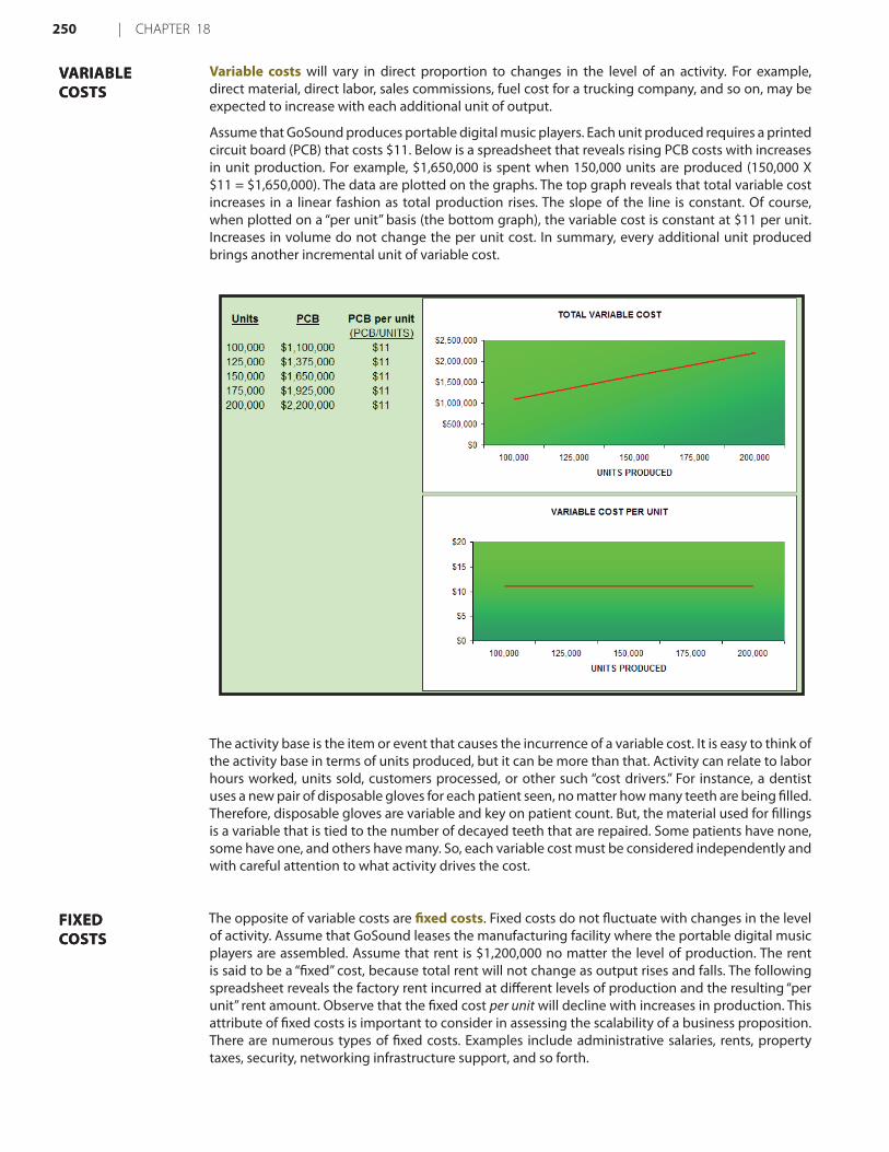
Below is an excerpt from an online catalog (Digi-Key Corporation). This is a pricing table for surface mount Zener Diodes. Notice that they are $0.44 each, or $3.00 for ten units, or $20.80 for 100 units, or $92.00 per thousand. The bottom line here is that they range from $0.44 down to $0.092 each, depending on the quantity purchased. This is quite a remarkable spread.

Digi-Key Part Number BZX84C36-FDICT-ND Price Break 1 10 100 250 500 1000

Unit Price 0.44000 0.30000 0.20800 0.15000 0.11200 0.09200

Price 0.44 3.00

20.80 37.50 56.00 92.00

Manufacturer Part Number BZX84C36-7-F

Description Diode Zener 300MW 36V SOT 23

Quantity Available 2896

Despite the wild spread in pricing, if your business needed about 150 of these diodes in your production process, you would study the above table and determine that the best quantity for you to order would be priced at $20.80 per hundred. As a result, your per unit variable cost would be $0.208. The “relevant range” is the anticipated activity level at which you will perform. Any pricing data outside of this range is irrelevant and need not be considered. This enhanced concept of variable cost is portrayed in the following graphic:

The relevant range comes into play when considering fixed costs as well. Many fixed costs are only fixed for a certain level of production. For example, a machine or manufacturing plant can reach capacity. To increase production beyond a certain level, additional machinery (or a new plant, additional supervisors, etc.) must be deployed. This will cause a major step upward in the fixed cost. Fixed costs that behave in this fashion are also called step costs. These costs are illustrated by the following diagram. The key conceptual point is to note that fixed costs are only fixed over some particular range of activity, and moving outside that range can significantly alter the cost structure.


After grasping the concepts of variable and fixed costs, it is important to understand their full implications in managing a business. Let’s first give added thought to fixed cost concepts. In an ideal setting, you would try to produce at the right-most edge of a fixed-cost step. This squeezes maximum productive output from a given level of expenditure. For a machine, it is as simple as running at full capacity. However, for a business with many fixed costs, it is more challenging to orchestrate operations so that each component is fully utilized.

Some fixed costs are committed fixed costs arising from an organization’s commitment to engage in operations. These elements include such items as depreciation, rent, insurance, property taxes, and the like. These costs are not easily adjusted with changes in business activity. On the other hand, discretionary fixed costs originate from top management’s yearly spending decisions; proper planning can result in avoidance of these costs if cutbacks become necessary or desirable. Examples of discretionary fixed costs include advertising, employee training, and so forth. Committed fixed costs relate to the desired long-run positioning of the firm; whereas, discretionary fixed costs have a short-term orientation. Committed fixed costs are important because they cannot be avoided in lean times; discretionary fixed costs can be altered with proper planning. Of course, a company should be careful to avoid incurring excessive committed fixed costs.

Variable costs are also subject to adjustment. In the Digi-Key Corporation example, it was illustrated how such costs can vary based on quantities ordered. Perhaps it occurred to you that one might order and store large quantities of the diodes for use in future periods (after all, 1200 units at $.208 each > 3000 units at $0.08 each). In a subsequent chapter, you will learn how to calculate economic order quantities that take into account carrying and ordering costs in balancing these important considerations. Even direct labor cost can be subject to adjustment for overtime premiums, based on whether or not overtime is worked. It may or may not make sense to meet customer demand by ramping up production when overtime premiums kick in. Later in this book, you will learn how to perform incremental analysis for such decision tasks.

The interplay between all of the different costs emphasizes the importance of good planning. The trick is to synchronize operations so that the benefits of each fixed cost are maximized, and variable cost patterns are established in the most economic position. All of this must be weighed against revenue opportunities; you must be able to sell what you produce. Some advanced managerial accounting courses present sophisticated linear programming models that take into account constraints and opportunities and project the ideal firm positioning. Those models are beyond the scope of an introductory class, but a number of simpler tools are available, and will be covered next.

Good managers must not only be able to understand the conceptual underpinnings of cost behavior, but they must also be able to apply those concepts to real world data that do not always behave in the expected manner. Cost data are impacted by complex interactions. Consider for instance the costs of operating a vehicle. Conceptually, fuel usage is a variable cost that is driven by miles. But, the efficiency of fuel usage can fluctuate based on highway miles versus city miles. Beyond that, tires wear faster at higher speeds, brakes suffer more from city driving, and on and on. Vehicle insurance is seen as a fixed cost; but portions are required (liability coverage) and some portions are not (collision coverage). Furthermore, if you have a wreck or get a ticket, your cost of coverage can rise. Now, the point is that assessing the actual character of cost behavior can be more daunting than you might first suspect. Nevertheless, management must understand cost behavior, and this sometimes takes a bit of forensic accounting work. Let’s begin by considering the case of “mixed costs.”

DIALING IN YOUR BUSINESS MODELDIALING IN YOUR BUSINESS MODEL

COST BEHAVIOR ANALYSIS

COST BEHAVIOR ANALYSIS

254 | CHAPTER 18

Many costs contain both variable and fixed components. These costs are called mixed or semi-variable. If you have a cell phone, you probably know more than you wish about such items. Cell phone agreements usually provide for a monthly fee plus usage charges for excess minutes, text messages, and so forth. With a mixed cost, there is some fixed amount plus a variable component tied to an activity. Mixed costs are harder to evaluate, because they change in response to fluctuations in volume. But, the fixed cost element means the overall change is not directly proportional to the change in activity.

To illustrate, assume that Butler’s Car Wash has a contract for its water supply that provides for a flat monthly meter charge of $1,000, plus $3 per thousand gallons of usage. This is a classic example of a mixed cost. Below is a graphic portraying Butler’s potential water bill, keyed to gallons used:

Look closely at the data in the spreadsheet, and notice that the “variable” portion of the water cost is $3 per thousand gallons. For example, spreadsheet cell B12 is $2,100 (700 thousand gallons at $3 per thousand); observe the formula for cell B12 in the upper bar of the spreadsheet (=(A12/1000)*3). In addition, the “fixed” cost is $1,000, regardless of the gallons used. The total in column D is the summation of columns B and C. The cost components are mapped in the diagram at the right.

Hopefully, the preceding illustration is clear enough. But, what if you were not given the “formula” by which the water bill is calculated? Instead, all you had was the information from a handful of past water bills. How hard would it be to to sort it out? Could you estimate how much the water bill should be for a particular level of usage? This type of problem is frequently encountered in business, as many expenses (individually and by category) contain both fixed and variable components.

One approach to sorting out mixed costs is the high-low method. It is perhaps the simplest technique for separating a mixed cost into fixed and variable portions. However, beware that it can return an imprecise answer if the data set under analysis has a number of rogue data points. But, it will work fine in other cases, as with the water bills for Butler’s Car Wash.

Information from Butler’s actual water bills is shown at left. Butler is curious to know how much the August water bill will be if 650,000 gallons are used. Assume that the only data available are from the aforementioned four water bills.

With the high-low technique, the highest and lowest levels of activity are identified for a period of time. The highest water bill is $3,550, and the lowest is $2,020. The difference in cost between the highest and lowest level of activity represents the variable cost ($3,550 - $2,020 = $1,530) associated with the change in activity (850,000 gallons on the high end and 340,000 gallons on the low end

MIXED COSTSMIXED COSTS

HIGH-LOW METHODHIGH-LOW METHOD

Apri l 450,000 gal lons $2,350

May 340,000 gal lons $2,020

June 850,000 gal lons $3,550

July 500,000 gal lons $2,500


yields a 510,000 gallon difference). The cost difference is divided by the activity difference to determine the variable cost for each additional unit of activity ($1,530/510 thousand gallons = $3 per thousand). The fixed cost can be calculated by subtracting variable cost (per-unit variable cost multiplied by the activity level) from total cost. The table at right reveals the application of the high-low method.

An electronic spreadsheet can be used to simplify the high-low calculations. The website includes a link to an illustrative spreadsheet for Butler.

As cautioned, the high-low method can be quite misleading. The reason is that cost data are rarely as linear as presented in the preceding illustration, and inferences are based on only two observations (either of which could be a statistical anomaly or “outlier”). For most cases, a more precise analysis tool should be used. If you have studied statistical methods, recall “regression analysis” or the “method of least squares.” This tool is ideally suited to cost behavior analysis. This method appears to be imposingly complex, but it is not nearly so complex as it seems. Let’s start by considering the objective of this calculation.

The goal of least squares is to define a line so that it fits through a set of points on a graph, where the cumulative sum of the squared distances between the points and the line is minimized (hence, the name “least squares”). Simply, if you were laying out a straight train track between a lot of cities, least squares would define a straight-line route between all of the cities, so that the cumulative distances (squared) from each city to the track is minimized.

Let’s dissect this method, beginning with the definition of a line. A line on a graph can be defined by its intercept with the vertical (Y) axis and the slope along the horizontal (X) axis. In the following diagram, observe a red line starting on the Y axis (at the value of “2”), and rising gently upward as it moves out along the X axis. The rate of rise is called the slope of the line; in this case, the slope is 0.8, because the line “rises” 8 units on the Y axis for every 10 units of “run” along the X axis.

METHOD OF LEAST SQUARESMETHOD OF LEAST SQUARES

USAGE

(in thousands of gal lons) COST

Highest levelLowest levelDifference

850340510

$ 3,550 2,020$ 1,530

Variable Cost per unit :($1,530/510) $3

HIGH LOW

Total costLess: Variable cost($3 per unit X usage)Fixed cost

$ 3,550

2,550 $ 1,000

$ 2,020

1,020 $ 1,000

256 | CHAPTER 18

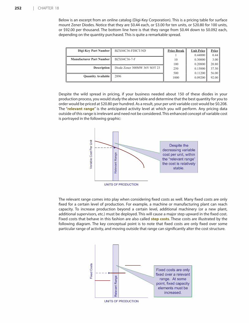
In general, a straight line can be defined by this formula:

Y = a + bX

where:

a = the intercept on the Y axis

b = the slope of the lineX = the position on the X axis

For the line drawn on the previous page, the formula would be:

Y = 2 + 0.8X

And, if you wished to know the value of Y, when X is 5 (see the red circle on the line), you perform the following calculation:

Y = 2 + (0.8 * 5) = 6

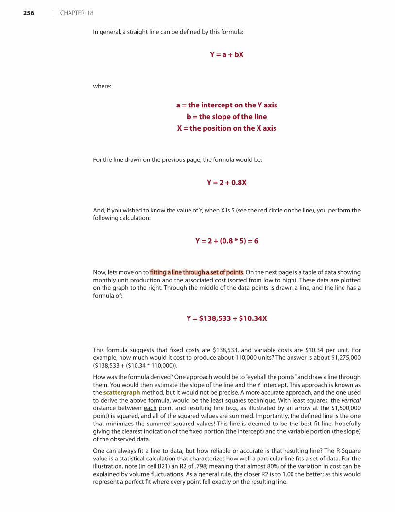
Now, lets move on to fitting a line through a set of points. On the next page is a table of data showing monthly unit production and the associated cost (sorted from low to high). These data are plotted on the graph to the right. Through the middle of the data points is drawn a line, and the line has a formula of:

Y = $138,533 + $10.34X

This formula suggests that fixed costs are $138,533, and variable costs are $10.34 per unit. For example, how much would it cost to produce about 110,000 units? The answer is about $1,275,000 ($138,533 + ($10.34 * 110,000)).

How was the formula derived? One approach would be to “eyeball the points” and draw a line through them. You would then estimate the slope of the line and the Y intercept. This approach is known as the scattergraph method, but it would not be precise. A more accurate approach, and the one used to derive the above formula, would be the least squares technique. With least squares, the vertical distance between each point and resulting line (e.g., as illustrated by an arrow at the $1,500,000 point) is squared, and all of the squared values are summed. Importantly, the defined line is the one that minimizes the summed squared values! This line is deemed to be the best fit line, hopefully giving the clearest indication of the fixed portion (the intercept) and the variable portion (the slope) of the observed data.

One can always fit a line to data, but how reliable or accurate is that resulting line? The R-Square value is a statistical calculation that characterizes how well a particular line fits a set of data. For the illustration, note (in cell B21) an R2 of .798; meaning that almost 80% of the variation in cost can be explained by volume fluctuations. As a general rule, the closer R2 is to 1.00 the better; as this would represent a perfect fit where every point fell exactly on the resulting line.


The R-Square method is good in theory. But, how does one go about finding the line that results in a minimization of the cumulative squared distances from the points to the line? One way is to utilize built-in tools in spreadsheet programs, as illustrated above. Notice that the formula for cell B21 (as noted at the top of spreadsheet) contains the function RSQ(C5:C16,B5:B16). This tells the spreadsheet to calculate the R2 value for the data in the indicated ranges. Likewise, cell B20 is based on the function SLOPE(C5:C16,B5:B16). Cell B19 is INTERCEPT(C5:C16,B5:B16). Most spreadsheets provide intuitive pop-up windows with prompts for setting up these statistical functions.

Spreadsheets have not always been available. You may be curious to know the underlying mechanics for the least squares method. If so, you can check out the link on the website.

Before moving on, let’s review a few key points. A good manager must understand an organization’s cost structure. This requires careful consideration of variable and fixed cost components. However, it is sometimes difficult to discern the exact cost structure. As a result, various methods can be employed to analyze cost behavior. Once an organization’s cost structure is understood, it then becomes possible to perform important diagnostic calculations which are the subject of the next sections of this chapter.

CVP analysis is imperative for management. It is used to build an understanding of the relationship between costs, business volume, and profitability. The analysis focuses on the interplay of pricing, volume, variable and fixed costs, and product mix. This analysis will drive decisions about what products to offer, how to price them, and how to manage an organization’s cost structure. CVP is at the heart of techniques that are useful for calculating the break-even point, volume levels necessary to achieve targeted income levels, and similar computations. The starting point for these calculations is to consider the contribution margin.

RECAPRECAP

BREAK-EVEN AND TARGET INCOME

BREAK-EVEN AND TARGET INCOME

258 | CHAPTER 18

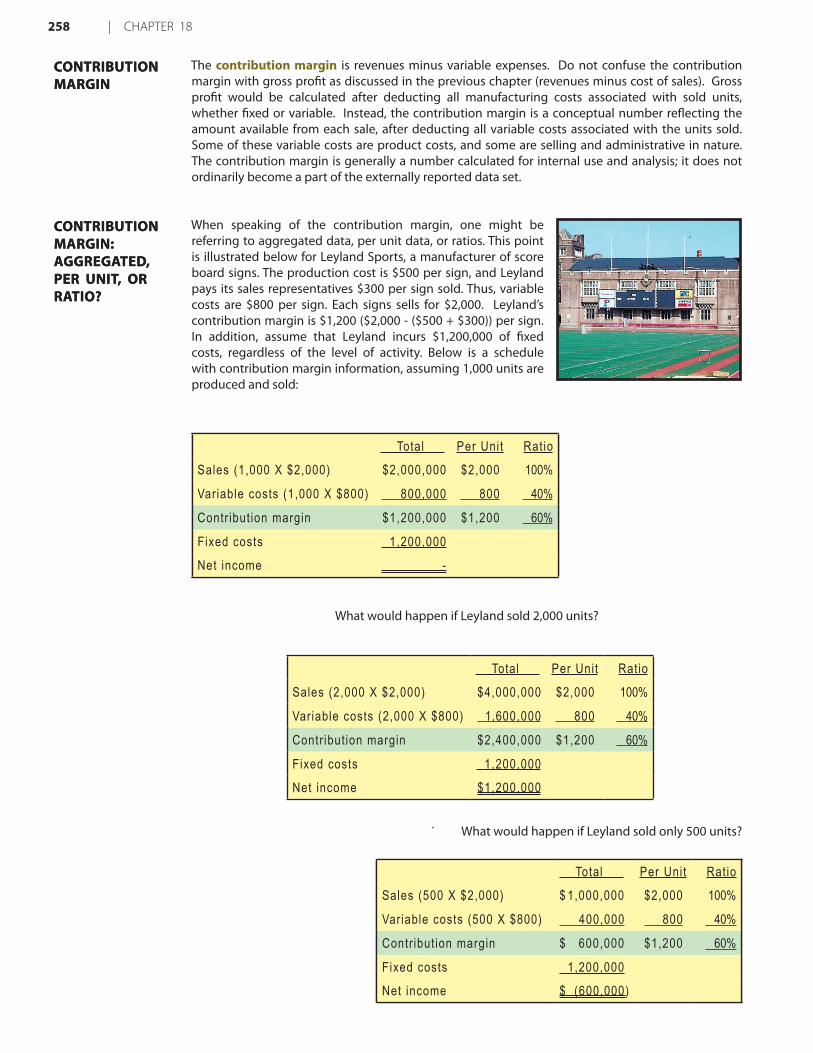
The contribution margin is revenues minus variable expenses. Do not confuse the contribution margin with gross profit as discussed in the previous chapter (revenues minus cost of sales). Gross profit would be calculated after deducting all manufacturing costs associated with sold units, whether fixed or variable. Instead, the contribution margin is a conceptual number reflecting the amount available from each sale, after deducting all variable costs associated with the units sold. Some of these variable costs are product costs, and some are selling and administrative in nature. The contribution margin is generally a number calculated for internal use and analysis; it does not ordinarily become a part of the externally reported data set.

When speaking of the contribution margin, one might be referring to aggregated data, per unit data, or ratios. This point is illustrated below for Leyland Sports, a manufacturer of score board signs. The production cost is $500 per sign, and Leyland pays its sales representatives $300 per sign sold. Thus, variable costs are $800 per sign. Each signs sells for $2,000. Leyland’s contribution margin is $1,200 ($2,000 - ($500 + $300)) per sign. In addition, assume that Leyland incurs $1,200,000 of fixed costs, regardless of the level of activity. Below is a schedule with contribution margin information, assuming 1,000 units are produced and sold:

What would happen if Leyland sold 2,000 units?

What would happen if Leyland sold only 500 units?

CONTRIBUTION MARGINCONTRIBUTION MARGIN

CONTRIBUTION MARGIN: AGGREGATED, PER UNIT, OR RATIO?

CONTRIBUTION MARGIN: AGGREGATED, PER UNIT, OR RATIO?

Total Per Unit Ratio

Sales (1,000 X $2,000) $2,000,000 $2,000 100%

Variable costs (1,000 X $800) 800,000 800 40%

Contr ibut ion margin $1,200,000 $1,200 60%

Fixed costs 1,200,000

Net income -


Sales (1,000 X $2,000) $2,000,000 $2,000 100%

Variable costs (1,000 X $800) 800,000 800 40%



Net income -


Sales (500 X $2,000) $ 1,000,000 $2,000 100%

Variable costs (500 X $800) 400,000 800 40%

Contr ibut ion margin $ 600,000 $1,200 60%


Net income $ (600,000)


Sales (500 X $2,000) $ 1,000,000 $2,000 100%

Variable costs (500 X $800) 400,000 800 40%

Contr ibut ion margin $ 600,000 $1,200 60%


Net income $ (600,000)


Sales (2,000 X $2,000) $4,000,000 $2,000 100%

Variable costs (2,000 X $800) 1,600,000 800 40%



Net income $1,200,000


Notice that changes in volume only impact certain amounts within the “total column.” Volume changes did not impact fixed costs, or change the per unit or ratio calculations. By reviewing the data on the previous page, also note that 1,000 units achieved breakeven net income. At 2,000 units, Leyland managed to achieve a $1,200,000 net income. Conversely, 500 units resulted in a $600,000 loss.

Leyland’s management would probably find the following chart very handy. Dollars are represented on the vertical axis and units on the horizontal:

Be sure to examine this chart, taking note of the following items:

The total sales line starts at “0” and rises $2,000 for each additional unit.

The total cost line starts at $1,200,000 (reflecting the fixed cost), and rises $800 for each additional unit (reflecting the addition of variable cost).

“Break-even” results where sales equal total costs.

At any given point, the width of the loss area (in red) or profit area (in green) is the difference between sales and total costs.

As they say, a picture is worth a thousand words, and that is certainly true for the CVP graphic just presented. However, everyone is not an artist, and you may find it more precise to do a little algebra to calculate the break-even point. Consider that:

Break-even results when:

Sales = Total Variable Costs + Total Fixed Costs

For Leyland, the math turns out this way:

(Units X $2,000) = (Units X $800) + $1,200,000

•

•

•

•

GRAPHIC PRESENTATIONGRAPHIC PRESENTATION

BREAK-EVEN CALCULATIONSBREAK-EVEN CALCULATIONS

260 | CHAPTER 18

Solving:

Step a: (Units X $2,000) = (Units X $800) + $1,200,000Step b: (Units X $1,200) = $1,200,000Step c: Units = 1,000

Now, it is possible to “jump to step b” above by dividing the fixed costs by the contribution margin per unit. Thus, a break-even short cut is:

Break-Even Point in Units = Total Fixed Costs / Contribution Margin Per Unit

1,000 Units = $1,200,000 / $1,200

Sometimes, you may want to know the break-even point in dollars of sales (rather than units). This approach is especially useful for companies with more than one product, where those products all have a similar contribution margin ratio:

Break-Even Point in Sales = Total Fixed Costs / Contribution Margin Ratio

$2,000,000 = $1,200,000 / 0.60

Breaking even is not a bad thing, but hardly a satisfactory outcome for most businesses. Instead, a manager may be more interested in learning the necessary sales level to achieve a targeted profit. The approach to solving this problem is to treat the “target income” like an added increment of fixed costs. In other words, the margin must cover the fixed costs and the desired profit:

Target Income results when:

Sales = Total Variable Costs + Total Fixed Costs + Target Income

Assume Leyland wants to know the level of sales to reach a $600,000 income:

(Units X $2,000) = (Units X $800) + $1,200,000 + $600,000

Solving:

Step a: (Units X $2,000) = (Units X $800) + $1,200,000 + $600,000Step b: (Units X $1,200) = $1,800,000Step c: Units = 1,500

TARGET INCOME CALCULATIONSTARGET INCOME CALCULATIONS


Again, it is possible to “jump to step b” by dividing the fixed costs and target income by the per unit contribution margin:

Units to Achieve a Target Income =

(Total Fixed Costs + Target Income) / Contribution Margin Per Unit

1,500 Units = $1,800,000 / $1,200

If you want to know the dollar level of sales to achieve a target net income:

Sales to Achieve a Target Income =

(Total Fixed Costs + Target Income) / Contribution Margin Ratio

$3,000,000 = $1,800,000 / 0.60

CVP is more than just a mathematical tool to calculate values like the break-even point. It can be used for critical evaluations about business viability.

For instance, a manager should be aware of the “margin of safety.” The margin of safety is the degree to which sales exceed the break-even point. For Leyland, the degree to which sales exceed $2,000,000 (its break-even point) is the margin of safety. This will give a manager valuable information as they plan for inevitable business cycles.

A manager should also understand the scalability of the business. This refers to the ability to grow profits with increases in volume. Compare the income analysis for Leaping Lemming Corporation and Leaping Leopard Corporation:

Both companies “broke even” in 20X1. Which company would you rather own? If you knew that each company was growing rapidly and expected to double sales each year (without any change in cost structure), which company would you prefer? With the added information, you would expect the following outcomes for 20X2:

CRITICAL THINKING ABOUT CVP

CRITICAL THINKING ABOUT CVP

LEAPING LEMMING CORPORATIONContr ibut ion-based Income Analysis for 20X1

Sales (5000 X $1,000) $5,000,000 100%Variable costs (5,000 X $900) 4,500,000 90%Contr ibut ion margin $ 500,000 10%Fixed costs 500,000 Net income $ -

LEAPING LEOPARD CORPORATIONContr ibut ion-based Income Analysis for 20X1

Sales (5000 X $1,000) $5,000,000 100%Variable costs (5,000 X $400) 2,000,000 40%Contr ibut ion margin $3,000,000 60%Fixed costs 3,000,000 Net income $ -

LEAPING LEMMING CORPORATIONContr ibut ion-based Income Analysis for 20X2

Sales (10,000 X $1,000) $10,000,000 100%Variable costs (10,000 X $900) 9,000,000 90%Contr ibut ion margin $ 1,000,000 10%Fixed costs 500,000 Net income $ 500,000

LEAPING LEOPARD CORPORATIONContr ibut ion-based Income Analysis for 20X2

Sales (10,000 X $1,000) $10,000,000 100%Variable costs (10,000 X $400) 4,000,000 40%Contr ibut ion margin 6,000,000 60%Fixed costs 3,000,000 Net income $ 3,000,000

262 | CHAPTER 18

This analysis reveals that Leopard has a more scalable business model. Its contribution margin is high and once it clears its fixed cost hurdle, it will turn very profitable. Lemming is fighting a never ending battle; sales increases are met with significant increases in variable costs. Be aware that scalability can be a double-edged sword. Pull backs in volume can be devastating to companies like Leopard because the fixed cost burden can be consuming. Whatever the situation, managers need to be fully cognizant of the effects of changes in scale on the bottom-line performance.

The only sure thing is that nothing is a sure thing. Cost structures can be anticipated to change over time. Management must carefully analyze these changes to manage profitability. CVP is useful for studying sensitivity of profit for shifts in fixed costs, variable costs, sales volume, and sales price.

Changes in fixed costs are perhaps the easiest to analyze. To determine a revised break-even level requires that the new total fixed cost be divided by the contribution margin. Let’s return to the example for Leyland Sports. Recall one of the original break-even calculations:


$2,000,000 = $1,200,000 / 0.60

If Leyland added a sales manager at a fixed salary of $120,000, the revised break-even would be:

$2,200,000 = $1,320,000 / 0.60

In this case, the fixed cost increased from $1,200,000 to $1,320,000, and sales must reach $2,200,000 to break even. This increase in break-even means that the manager needs to produce at least $200,000 of additional sales to justify their post.

In recruiting the new sales manager, Leyland became interested in an aggressive individual who was willing to take the post on a “4% of sales” commission-only basis. Let’s see how this would change the breakeven point:


$2,142,857 = $1,200,000 / 0.56

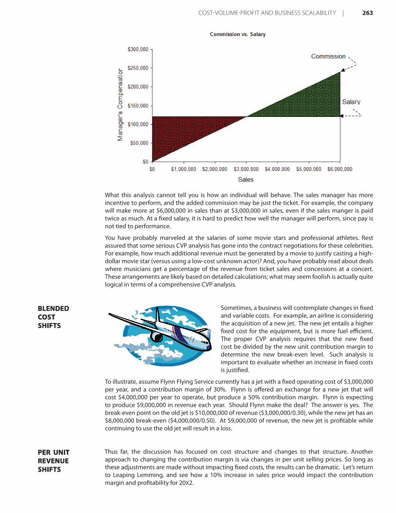
This calculation uses the revised contribution margin ratio (60% - 4% = 56%), and produces a lower break-even point than with the fixed salary ($2,142,857 vs. $2,200,000). But, do not assume that a lower break-even defines the better choice! Consider that the lower contribution margin will “stick” no matter how high sales go. At the upper extremes, the total compensation cost will be much higher with the commission-based scheme. Following is a graph of commission cost versus salary cost at different levels of sales. You can see that the commission begins to exceed the fixed salary at any point above $3,000,000 in sales. In fact, at $6,000,000 of sales, the manager’s compensation is twice as high if commissions are paid in lieu of the salary!

SENSITIVITY ANALYSISSENSITIVITY ANALYSIS

CHANGING FIXED COSTSCHANGING FIXED COSTS

CHANGING VARIABLE COSTS

CHANGING VARIABLE COSTS


What this analysis cannot tell you is how an individual will behave. The sales manager has more incentive to perform, and the added commission may be just the ticket. For example, the company will make more at $6,000,000 in sales than at $3,000,000 in sales, even if the sales manger is paid twice as much. At a fixed salary, it is hard to predict how well the manager will perform, since pay is not tied to performance.

You have probably marveled at the salaries of some movie stars and professional athletes. Rest assured that some serious CVP analysis has gone into the contract negotiations for these celebrities. For example, how much additional revenue must be generated by a movie to justify casting a high-dollar movie star (versus using a low-cost unknown actor)? And, you have probably read about deals where musicians get a percentage of the revenue from ticket sales and concessions at a concert. These arrangements are likely based on detailed calculations; what may seem foolish is actually quite logical in terms of a comprehensive CVP analysis.

Sometimes, a business will contemplate changes in fixed and variable costs. For example, an airline is considering the acquisition of a new jet. The new jet entails a higher fixed cost for the equipment, but is more fuel efficient. The proper CVP analysis requires that the new fixed cost be divided by the new unit contribution margin to determine the new break-even level. Such analysis is important to evaluate whether an increase in fixed costs is justified.

To illustrate, assume Flynn Flying Service currently has a jet with a fixed operating cost of $3,000,000 per year, and a contribution margin of 30%. Flynn is offered an exchange for a new jet that will cost $4,000,000 per year to operate, but produce a 50% contribution margin. Flynn is expecting to produce $9,000,000 in revenue each year. Should Flynn make the deal? The answer is yes. The break-even point on the old jet is $10,000,000 of revenue ($3,000,000/0.30), while the new jet has an $8,000,000 break-even ($4,000,000/0.50). At $9,000,000 of revenue, the new jet is profitable while continuing to use the old jet will result in a loss.

Thus far, the discussion has focused on cost structure and changes to that structure. Another approach to changing the contribution margin is via changes in per unit selling prices. So long as these adjustments are made without impacting fixed costs, the results can be dramatic. Let’s return to Leaping Lemming, and see how a 10% increase in sales price would impact the contribution margin and profitability for 20X2.

BLENDED COST SHIFTS

BLENDED COST SHIFTS

PER UNIT REVENUE SHIFTS

PER UNIT REVENUE SHIFTS

264 | CHAPTER 18

Notice that this 10% increase in price results in a doubling of the contribution margin and a tripling of the net income. Bingo: the solution to increasing profits is to raise prices while maintaining the existing cost structure -- if it were only this easy! Customers are sensitive to pricing and even a small increase can drive customers to competitors. Before raising prices, a company must consider the “price elasticity” of demand for its product. This is fancy jargon to describe the simple reality that demand for a product will drop as its price rises.

So, the real question for Leaping Lemming is to assess how much volume drop can be absorbed when prices are increased. The appropriate analysis requires dividing the continuing fixed costs (plus target or current net income) by the revised unit contribution margin; this results in the required sales (in units) to maintain the current level of profitability. For Lemming to achieve a $500,000 profit level at the revised pricing level, it would need to sell 5,000 units:

Units to Achieve a Target Income =

(Total Fixed Costs + Target Income) / Contribution Margin Per Unit

5,000 Units = ($500,000 + $500,000) / $200

If Lemming sells at least 5,000 units at $1,100 per unit, it will make at least as much as it would by selling 10,000 units at $1,000 per unit. The unknown is what customer response will be to the $1,100 pricing decision. Many a business has fallen prey to the presumption that they could raise prices with impunity; others have scored homeruns by getting away with such increases.

Some contracts provide for “cost plus” pricing, or similar arrangements that seek to provide the seller with an assured margin. These agreements are intended to allow the seller a normal and fair profit margin, and no more. However, they can have unintended consequences. Let’s evaluate an example. Pioneer Plastics sells trash bags to Heap Compacting Service. Heap and Pioneer have entered into an agreement that provides Pioneer with a contribution margin of 20% on 1,000,000 bags. Originally, the bags were anticipated to cost Pioneer $1 each to produce, plus a fixed cost of $100,000. However, increases in petroleum products necessary to produce the bags skyrocketed, and Pioneer’s variable production cost was actually $3 per unit. Let’s see how Pioneer faired under their agreement:

$1 Scenario $3 scenarioSales $ 1,250,000 $ 3,750,000Variable costs (1,000,000 X $1 vs. $3) 1,000,000 3,000,000Contr ibut ion margin (20% of sales) $ 250,000 $ 750,000Fixed costs 100,000 100,000 Net income $ 150,000 $ 650,000

MARGIN BEWAREMARGIN BEWARE

LEAPING LEMMING CORPORATIONIncome Analysis for 20X2 at Alternative Pricing

$1,000 per unit scenario

$1,100 per unit scenario

Sales (10,000 units) $10,000,000 $11,000,000Variable costs (10,000 X $900) 9,000,000 9,000,000Contr ibut ion margin $ 1,000,000 $ 2,000,000Fixed costs 500,000 500,000 Net income $ 500,000 $ 1,500,000


Notice the astounding change in Pioneer’s net income - $150,000 versus $650,000. Such “cost plus” agreements must be carefully constructed, else the seller has little incentive to do anything but let costs creep up. Sometimes you will hear a company complain about cost increases negatively affecting their “margins;” before you assume the worst, take a closer look to see how the bottom line is being impacted. Even if Pioneer agreed to cut Heap a break and reduce their margin in half, their bottom line profit would still soar in the illustration.

In the preceding illustration, the contribution margin was 20% of sales. Accordingly, variable costs are 80% of sales. If total variable costs are $1,000,000, then sales would be $1,250,000 ($1,000,000 divided by 0.80).

How many businesses sell only one product? The reality is that firms usually offer a diverse product line, and the individual products will have different selling prices, contribution margins, and contribution margin ratios. Yet, the firm’s total fixed cost picture may be the same, no matter the mix of products sold. This can cloud the ability to perform simple CVP analysis. To lift this cloud requires some knowledge of the product mix.

Let’s assume Hummingbird Feeders produces and sells a brightly colored feeding container for $15 (variable cost of production is $10, and contribution margin is $5) and a nectar formula for $3 per packet ($1 variable cost to produce, resulting in a $2 contribution margin). Hummingbird Feeders sells 10 packets of nectar for every feeder sold. Its fixed cost is $100,000. How many feeders and packets must be sold to break even? To answer this question requires a redefinition of the “unit.” If we assume the “unit” is 1 feeder and 10 packets, we would then see that each “unit” would have a contribution margin of $25, as shown below.

Contribution MarginFeeder 1 item @ $5 = $5.00Nectar Packets 10 items @ $2 each = 20.00“Unit” contr ibut ion $25.00

To recover $100,000 of fixed cost, at $25 of contribution per “unit,” would require selling 4,000 “units” ($100,000/$25). To be clear, this translates into 4,000 feeders and 40,000 packets of nectar. Total break-even sales would be $180,000 (($15 X 4,000 feeders) + ($3 X 40,000 packets)). Of course, the validity of this analysis depends upon actual sales occurring in the predicted ratio. Changes in product mix will result in changes in break-even levels. If Hummingbird Feeders sold $180,000 in feeders, and no packets of nectar, they would come no where near breakeven (because the contribution margin ratio on feeders is much lower than on the packets of nectar).

Note that one could also get the $180,000 result by dividing the fixed cost by the weighted-average contribution margin ($100,000/0.555 = $180,000). The weighted-average contribution margin of 0.555 is calculated as follows:

Product Sales to

Total Sales Ratio (mix)

Product Contr ibut ion Margin Ratio

Weighted Average

Ratio

Feeder (1 @ $15) $15/$45 X $5/$15 = 0.1111Nectar Packets (10 @ $3) $30/$45 X $2/$3 = 0.4444 0.5555

MARGIN MATHEMATICSMARGIN MATHEMATICS

CVP FOR MULTIPLE PRODUCTS

CVP FOR MULTIPLE PRODUCTS

266 | CHAPTER 18

Businesses must be mindful of the product mix. Automobile manufacturers have a broad range of products, some at high margin and some at lower levels. If customers unexpectedly substitute economy cars for sport utility vehicles, basic models for luxury models, etc., the resulting bottom line impacts can be significant. Product mix can also be important for companies that sell a base product and a related disposable. For example, a printer manufacturer may sell “unprofitable” printers along with large quantities of high margin ink cartridges. Managers of such businesses need to watch not only total sales, but also keep a keen eye on the product mix.

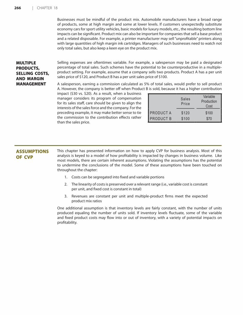
Selling expenses are oftentimes variable. For example, a salesperson may be paid a designated percentage of total sales. Such schemes have the potential to be counterproductive in a multiple-product setting. For example, assume that a company sells two products. Product A has a per unit sales price of $120, and Product B has a per unit sales price of $100.

A salesperson, earning a commission calculated as 5% of total sales, would prefer to sell product A. However, the company is better off when Product B is sold, because it has a higher contribution impact ($30 vs. $20). As a result, when a business manager considers its program of compensation for its sales staff, care should be given to align the interests of the sales force and the company. For the preceding example, it may make better sense to tie the commission to the contribution effects rather than the sales price.

This chapter has presented information on how to apply CVP for business analysis. Most of this analysis is keyed to a model of how profitability is impacted by changes in business volume. Like most models, there are certain inherent assumptions. Violating the assumptions has the potential to undermine the conclusions of the model. Some of these assumptions have been touched on throughout the chapter:

Costs can be segregated into fixed and variable portions

The linearity of costs is preserved over a relevant range (i.e., variable cost is constant per unit, and fixed cost is constant in total)

Revenues are constant per unit and multiple-product firms meet the expected product mix ratios

One additional assumption is that inventory levels are fairly constant, with the number of units produced equaling the number of units sold. If inventory levels fluctuate, some of the variable and fixed product costs may flow into or out of inventory, with a variety of potential impacts on profitability.

1.

2.

3.

MULTIPLE PRODUCTS, SELLING COSTS, AND MARGIN MANAGEMENT

MULTIPLE PRODUCTS, SELLING COSTS, AND MARGIN MANAGEMENT

ASSUMPTIONS OF CVPASSUMPTIONS OF CVP

Sales Price

Variable Production

CostPRODUCT A $120 $100PRODUCT B $100 $70

Cost Volume Profit Analysis

Documents

unit cost

fuel cost

cost drivers

total variable cost

cost behavior patterns

cost behavior profitability

business growth

specific business