Cost Performance Index of Temporary Erosion Control Products

Technical Report Documentation Page 1. Report No. FHWA/TX-08/0-5309-1

2. Government Accession No.

3. Recipient's Catalog No. 5. Report Date May 2007 Published: October 2007

4. Title and Subtitle COST PERFORMANCE INDEX OF TEMPORARY EROSION CONTROL PRODUCTS

6. Performing Organization Code

7. Author(s) Jett McFalls, Ming-Han Li, Young-Jae Yi, and Harlow C. Landphair

8. Performing Organization Report No. Report 0-5309-1 10. Work Unit No. (TRAIS)

9. Performing Organization Name and Address Texas Transportation Institute The Texas A&M University System College Station, Texas 77843-3135

11. Contract or Grant No. Project 0-5309 13. Type of Report and Period Covered Technical Report: September 2005-August 2006

12. Sponsoring Agency Name and Address Texas Department of Transportation Research and Technology Implementation Office P.O. Box 5080 Austin, Texas 78763-5080

14. Sponsoring Agency Code

15. Supplementary Notes Project performed in cooperation with the Texas Department of Transportation and the Federal Highway Administration. Project Title: Develop Guidance for Selecting and Cost-Effective Application of Temporary Erosion Control Methods URL: http://tti.tamu.edu/document/0-5309-1.pdf 16. Abstract The objective of this research project was to develop a cost-performance index (CPI) for products in the Texas Department of Transportation’s (TxDOT’s) Approved Products List (APL). TxDOT’s APL was created from performance testing conducted in the Hydraulics, Sedimentation, and Erosion Control Laboratory (HSECL) of the Texas Transportation Institute (TTI). The performance testing includes sediment loss and vegetation growth. Both slope protection and channel protection products are evaluated. The intention of developing the CPI was to further include cost data in the APL so that users of the APL can justify the use of a product based on the combined cost and performance information. Data used for the CPI development include surveyed cost from manufacturers, material composition and sediment loss performance data from TTI performance testing. The conceptual model of the CPI can be described as “the benefit of potential soil protection per unit cost of both product and potential topsoil replacement expense.” The benefit of potential soil protection is a hypothetical cost savings from slope or channel failure over the entire product lifespan. The potential topsoil replacement expense reflects the fact that soil loss will occur no matter how well the surface is protected. When soil is lost, there is a potential of topsoil replacement, which in turn costs money. With this concept, a typical topsoil price of $25 per cubic yard was used. The result of the project includes a series of tables listing products with high/medium CPI. Five project durations were used: temp (0-3 months), short (3-12 months), mid (12-24 months), long (24-36 months), and permanent (36-54 months). For slope protection products, two slopes and two soil types were included: 2:1 clay, 3:1 clay, 2:1 sand and 3:1 sand. For channel protection products, six shear stresses were used to separate different products: 0-2, 0-4, 0-6, 0-8, 0-10 and 0-12 lb/ft2. The improved APL will enable erosion control designers and specifiers to select products best suited for different project durations with great cost-savings potential. 17. Key Words Cost Performance Index, Slope Protection, Channel Protection, Rolled Erosion Control Products, Turf-Reinforcement Mats

18. Distribution Statement No restrictions. This document is available to the public through NTIS: National Technical Information Service Springfield, Virginia 22161 http://www.ntis.gov

19. Security Classif.(of this report) Unclassified

20. Security Classif.(of this page) Unclassified

21. No. of Pages 80

22. Price

Form DOT F 1700.7 (8-72) Reproduction of completed page authorized

http://www.ntis.gov

RESUBMITTAL

COST PERFORMANCE INDEX OF TEMPORARY EROSION CONTROL PRODUCTS

by

Jett McFalls Associate Transportation Researcher

Texas Transportation Institute

Ming-Han Li Assistant Research Engineer


Young-Jae Yi Graduate Research Assistant

Texas A&M University

and

Harlow C. Landphair Research Scientist


Report 0-5309-1 Project 0-5309

Project Title: Develop Guidance for Selecting and Cost-Effective Application of Temporary Erosion Control Methods

Performed in cooperation with the Texas Department of Transportation

and the Federal Highway Administration

May 2007 Published: October 2007

TEXAS TRANSPORTATION INSTITUTE

The Texas A&M University System College Station, Texas 77843-3135

RESUBMITTAL

v

DISCLAIMER

This research was performed in cooperation with the Texas Department of Transportation

(TxDOT) and the Federal Highway Administration (FHWA). The contents of this report reflect

the views of the authors, who are responsible for the facts and the accuracy of the data presented

herein. The contents do not necessarily reflect the official view or policies of the FHWA or

TxDOT. This report does not constitute a standard, specification, or regulation.

The United States Government and the State of Texas do not endorse products or

manufacturers. Trade or manufacturers’ names appear herein solely because they are considered

essential to the object of this report.

RESUBMITTAL

vi

ACKNOWLEDGMENTS

This project was conducted in cooperation with TxDOT and FHWA.

The authors of this report would like to thank Program Coordinator Dianna Noble,

Project Director Dennis Markwardt, and the Project Advisors Ben Bowers, Karl Bednarz, Norm

King, and David Zwernemann for their guidance and assistance throughout this project.

We would like to offer a special thanks to the following Texas Transportation Institute

personnel contributing to this report: Derrold Foster, Arnes Purdy, Cynthia Lowery, and Melissa

Marrero.

RESUBMITTAL

vii

TABLE OF CONTENTS

Page List of Figures............................................................................................................................... ix List of Tables ................................................................................................................................. x INTRODUCTION......................................................................................................................... 1

Background and Significance of Work....................................................................................... 1 Study Problem Statement........................................................................................................ 1 Current TxDOT Practice......................................................................................................... 2 Underlying Principles ............................................................................................................. 3 Approach to the Problem ........................................................................................................ 3

Implementation ........................................................................................................................... 4 LITERATURE REVIEW ............................................................................................................ 5

Performance of Erosion Control Measures................................................................................. 5 Performance of Rolled Erosion Control Products (RECPs) ................................................... 5 Performance of Soil Roughening............................................................................................ 7 Performance of Organic Measures (Composts and Mulches) ................................................ 7

Soil Erosion Factors.................................................................................................................. 10 Rainfall Erosivity (R)............................................................................................................ 10 Soil Erodibility (K) ............................................................................................................... 11 Slope Steepness and Length (LS) ......................................................................................... 12 Cover (C) .............................................................................................................................. 13 Erosion Control Practice (P) ................................................................................................. 14 Limitations of the USLE Model ........................................................................................... 14

METHODOLOGY ..................................................................................................................... 17 Data Collection and Treatment ................................................................................................. 17

Cost of Products on the Approved Product List ................................................................... 17 Soil Loss Data ....................................................................................................................... 18 Product Type (Classified by Material Composition and Longevity).................................... 22

Lifetime Soil Protection Performance ...................................................................................... 25 Lifetime Soil Protection by Product ..................................................................................... 25 Lifetime Soil Protection by Vegetation ................................................................................ 26

Cost-Performance Index ........................................................................................................... 29 Basic Concept ....................................................................................................................... 29 Cost-Performance Index for Slope Products......................................................................... 29 Cost-Performance Index for Channel Product...................................................................... 35

RESULTS .................................................................................................................................... 37 Descriptive Analysis of Erosion Control Products in the APL ................................................ 37

Slope Protection Products ..................................................................................................... 37 Channel Protection Products................................................................................................. 39

Cost-Performance Analysis ...................................................................................................... 42 Lifetime Performance of Erosion Control Products ............................................................. 42 Cost-Performance Index of Slope Protection Products ........................................................ 43 Cost-Performance Index of Channel Protection Products .................................................... 44

REFERENCES............................................................................................................................ 47 Appendix A.................................................................................................................................. 49

RESUBMITTAL

viii

Appendix B .................................................................................................................................. 55 Appendix C.................................................................................................................................. 59

RESUBMITTAL

ix

LIST OF FIGURES Page Figure 1: Nomograph Allowing a Quick Assessment of the "K" Factor Of Soil Erodibility....... 11 Figure 2: Relationship Among Erosion Level, And Slope Length And Steepness ...................... 13 Figure 3: An Example of Life-Performance Of Erosion Control Products. ................................. 26 Figure 4: An Example of Vegetation Performance with Different Establishing Times. .............. 27 Figure 5: Combination of Product and Vegetation Performance Lines in Slope ......................... 30 Figure 6: The Soil Loss Model of Product and Vegetation Combined for Slope Condition........ 31 Figure 7: Failure Prevention by Erosion Control Product (F). ..................................................... 33 Figure 8: The Soil Loss Model of Products and Vegetation Combined In Channel .................... 35 Figure 9: Price Index of Slope Protection Products (by product type). ........................................ 37 Figure 10: Soil Loss Index By Product Type In Clay Slope......................................................... 38 Figure 11: Soil Loss Index By Product Type In Sand Slope ........................................................ 39 Figure 12: Price Index by Product Type, Channel APL. .............................................................. 40 Figure 13: Soil Loss Index by Product Type @ Low Shear Stress. ............................................. 41 Figure 14: Soil Loss Index By Product Type @ Mid Shear Stress. ............................................. 41 Figure 15: Soil Loss Index by Product Type @ High Shear Stress.............................................. 42 Figure 16: Correlation between Price and Life-Performance of Slope Protection Products. ....... 43 Figure 17: Correlation between Price and Life-Performance of Channel Protection Products. ... 43

RESUBMITTAL

x

LIST OF TABLES Page Table 1: Soil Protection Effectiveness Of Selected BMPs. ............................................................ 6 Table 2: TxDOT/TTI Sediment Loss Thresholds........................................................................... 6 Table 3: Soil Protection Effectiveness of Soil Roughness.............................................................. 7 Table 4: Performance Test Results Obtained from Various Studies .............................................. 8 Table 5: Soil Protection Effectiveness of Organic Measures. ........................................................ 9 Table 6: Soil Erodibility Guide..................................................................................................... 12 Table 7: Survey Response Rate. ................................................................................................... 17 Table 8: Ratio of Field Soil Loss Data to Indoor Soil Loss Data of The HSECL. ....................... 18 Table 9: Threshold Of TxDOT APL Slope Test........................................................................... 20 Table 10: Threshold Of TxDOT APL Channel Test .................................................................... 20 Table 11: Soil Loss Index and Corresponding Soil Loss Range for Slope Protection Products. . 21 Table 12: Soil Loss Index and Corresponding Soil Loss Range for Channel Protection Products

............................................................................................................................................... 21 Table 13: Classification of Product Type. .................................................................................... 24 Table 14: The Ratio of Soil Loss to APL Threshold on Bare Soil Surface Condition. ................ 32 Table 15: Acceptable Price Threshold for Slope Protection Products.......................................... 44 Table 16: Acceptable Price Threshold for Channel Protection Products ..................................... 44

RESUBMITTAL

1

INTRODUCTION

BACKGROUND AND SIGNIFICANCE OF WORK

In order to maintain federal regulatory compliance and ensure that the most effective erosion

control products are used on its construction and maintenance projects, the Texas Department of

Transportation (TxDOT) bases material selection on an Approved Product List (APL). This

APL is based on field performance of the products through a formal evaluation program at the

TxDOT/Texas Transportation Institute (TTI) Hydraulics, Sedimentation, and Erosion Control

Laboratory (HSECL) at the Texas A&M University Riverside Campus. The two critical

performance factors identified are:

• how well the product protected the seedbed of an embankment and drainage channel

from the loss of sediment during simulated rainfall or channel flow events, and

• how well the product promoted the establishment of warm-season, perennial vegetation.

While these two factors are critical to erosion control performance, there has been no

consideration for material cost and longevity. Furthermore, there are potentially less expensive

erosion control techniques which have not previously been included in the approval process.

These techniques include crimped or tacked hay/straw, compost, slope tracking, wood mulch,

and soil binders. This project examined available performance and cost data of these non-

manufactured techniques in terms of cost, sediment loss prevention, and vegetation

establishment. This project also looked at the cost of current products on the APL in terms of

costs for the material, installation, maintenance, repair, and effectiveness, and developed a cost-

performance index. The objective of the effort is to provide guidance for selecting the most cost

effective erosion control materials and methods.

Study Problem Statement

In order to meet water quality mandates, TxDOT utilizes a number of products to control erosion

on construction projects throughout the state. The overall cost for the use of soil retention

blankets in construction projects in 2004 was 1.2 million dollars.

RESUBMITTAL

2

To ensure that products meet standard performance criteria TxDOT utilizes an APL, which is

based on an established testing program initiated by TxDOT in 1990. Since its creation, the

TxDOT APL has become a nationally recognized authority for the performance of temporary

erosion control materials. Products on the APL have passed the standard performance tests and,

if properly installed can be expected to perform the needed erosion control during construction.

TxDOT design engineers, inspectors, contractors, and even other state DOTs have benefited

from this program through the continuing FHWA pooled fund study sponsored by TxDOT.

In reviewing the 12 years of performance data developed by the HSECL, and comparing it to

some very recent tests on natural materials, it appears that the less expensive natural materials

have sediment reduction and vegetation establishment performance properties equivalent to the

manufactured rolled erosion control products (RECPs). For example, it is estimated that on

average, straw can be blown and crimped/tacked onto a slope at a cost of between $0.08 to $0.24

per square yard, as compared to RECPs that cost from $1.00 to $3.00 per square yard in place,

and will yield a similar level of protection. Therefore, it seems prudent to look closer at these

materials and begin to consider cost as a significant part of the process for recommending a

material for use by TxDOT.

Despite the recognition of the APL by erosion control professionals and its significant

contribution to date, there is room for improvement. First, cost information is not included in the

APL. Cost of materials, installation, and removal (if necessary) will further guide designers in

their selection of cost-effective products. Second, following the need for cost information is

further consideration of older technologies such as crimped straw, slope tracking, and compost

that may be just as effective and less expensive.

Current TxDOT Practice

Current TxDOT design references that address temporary soil erosion control are located in the

Standard Specification for Highways Streets and Bridges (TxDOT, 2004) and the APL. Using

this Standard Specification, designers can select the appropriate erosion control product based on

site conditions (slope steepness and soil type). The data used to select a product considers a

RESUBMITTAL

3

material’s ability to reduce sediment loss and establish vegetation. Data for material cost and

longevity are not used in the current APL evaluation procedure.

Underlying Principles

Researchers categorize temporary erosion control into two types: slope protection and channel

protection. Slope protection represent highway embankments and planar rights-of-way where

only overland or sheet flow will occur. Channel protection, where concentrated flow is the

result, produces greater erosive forces on the channel bed and sides. When these conditions are

encountered during construction, the appropriate type of erosion control material is essential.

There are three measures of performance considered for erosion control on slopes, they are:

reduction of rain impact on soil surface, reduction of sediment laden runoff, and establishment of

vegetation. While commercial RECPs listed on the APL can achieve such performance, non-

proprietary techniques such as soil roughing, surface terracing, crimped straw, and others, may

achieve the same results with lower costs and less maintenance. Figure 1 illustrates the basic

schematic erosion control mechanisms for slopes.

For channels, protection from shear stress exerted on the channel bottom and vegetation

establishment are the critical factors in determining a material’s suitability. The shear stress (τ)

on an open channel is expressed as τ= γds and is computed as the product of the slope of the

channel (s), fluid specific gravity (γ), and the depth of the flow (d) (Chow 1959). Common

techniques to control channel erosion include rock riprap, cabled blocks, and turf-reinforcing

mats (TRMs) which can be described as a high-strength RECP. For temporary channel erosion

control, a long-term TRM or temporary, bio-degradable channel liners are the most common

methods of protection.

Approach to the Problem

The objective of this project is to synthesize all the available data to develop a Cost-Performance

Index (CPI) for products currently on the APL, as well as several inexpensive alternative best

management practices (BMPs), including compost, crimped and tacked hay/straw, and soil

RESUBMITTAL

4

roughening. In addition, a standard procedure will be created so that future products or methods

can be evaluated and their CPI can be determined.

IMPLEMENTATION

The results of this project will provide TxDOT specific information necessary to determine the

cost effectiveness of various erosion control products and methods (both old and new), which

could result in a significant cost savings to the Department while improving compliance with

Federal storm water regulations.

Information generated by this study may form the basis for revising the current APL for erosion

control to include cost effectiveness. This revision would be a guide to assist in selecting the

most cost-effective practice or product. Once completed, the information will be included in the

current erosion control training curriculum (ENV102) offered by TxDOT.

RESUBMITTAL

5

LITERATURE REVIEW This literature review has two purposes:

• to introduce the performance of various erosion control measures including RECPs, soil

roughening and organic measures (composts and mulches), and

• to determine the most effective method to standardize the test results from various

erosion control studies using the Universal Soil Loss Equation (USLE) model.

This review can be summarized as follows.

• Erosion control performance without vegetation can be compared as:

RECPs > Mulch > Soil roughening > Compost • Soil roughening and compost may be combined with other measures such as

vegetation and mulch, which improves their performance. • Test conditions vary among studies making it difficult to standardize the test

results used to compare performance of the different products evaluated.

• The USLE cannot provide an ideal method to standardize tests conducted on

different conditions. The model was based on tests conducted on relatively flat

areas and ignored the impact of slope change in the erosion mechanism.

PERFORMANCE OF EROSION CONTROL MEASURES

Performance of Rolled Erosion Control Products (RECPs)

Based on indoor rainfall simulation tests, the California Department of Transportation

(CALTRANS) (2000) suggests that RECPs reduce more than 90 percent in soil loss on 2:1

clayey sand slopes (Table 1). The range of erosion control performance in CALTRANS’ study is

consistent with what has been observed in rainfall simulation testing for TxDOT APL at the

HSECL. TxDOT approves soil erosion products that can reduce soil loss at a minimum of 83

percent on 2:1 sand slope and 98 percent on 2:1 clay slope (Table 2). The test results of both test

facilities are comparable as they utilized similar facilities and test conditions except soil type and

rainfall scheme. The difference in effectiveness among different soil type (i.e. 83 percent at clay,

90 percent at clayey sand, and 98 percent at sand) indicates that RECPs are less effective in

erodible soils, that is, the effectiveness is higher at clay slope than sand slope.

RESUBMITTAL

6

Table 1: Soil Protection Effectiveness Of Selected BMPs.

Soil Stabilization Measure Average Erosion Reduction on Bare Soil 2:1 Clayey Sand (%)

Bonded fiber matrix 100% Straw blanket 98% Wood fiber blanket 98% Straw-coconut blanket 97% Straw incorporated 96% Coir blanket 94% Curled wood fiber blanket 91%

Rainfall:

Part1 – 5 mm/hr, 30 min Part2 – 40 mm/hr, 40 min Part3 – 5 mm/hr. 30 min(1)

One 3-part event (3 replicate plots)

(1) Corresponds to 10-yr storm in District 7 of California Adapted from Caltrans (2000)

Table 2: TxDOT/TTI Sediment Loss Thresholds.

Slope Condition

Soil loss Bare Soil (lb/100 ft2)

TxDOT APL Threshold (lb/100 ft2)

Erosion Reduction Bare Soil

(%)

2:1 Clay 350.0 7.9 98% 2:1 Sand 3885.3 631.8 84% 3:1 Clay 266.5 7.9 97% 3:1 Sand 1709.6 284.3 83%

Rainfall:

30.2 mm/hr, 10 min (twice) (1) 145.5 mm/hr, 10 min (twice) (1) 183.6 mm/hr, 10 min (twice) (1)

Six events run two weeks apart

(plots not replicate) (1) Corresponds to 1-yr, 2-yr, and 5-yr storms in Texas, respectively

RESUBMITTAL

7

Performance of Soil Roughening

CALTRANS (2000) tested the erosion control performance of soil roughening techniques

including imprinting, sheepsfoot-rolling, trackwalking, and ripping. The tests show that soil

roughening is less effective in erosion control than RECPs (Table 3). Soil roughening can be

combined with other erosion control measures including compost and mulch, making them

perform better. The imprinting technique demonstrated good performance at 2:1 clayey sand

slope (76 percent decrease in soil loss), which implies imprinting could be a candidate for

protecting 3:1 clay slopes.

Table 3: Soil Protection Effectiveness of Soil Roughness.

Soil Roughening Technique

Average Erosion Reduction from Bare Soil at 2:1 Clayey Sand (%)

Imprinted 76%

Sheepsfoot 55%

Trackwalked 52%

Ripped 12% Adapted from Caltrans (2000)

Performance of Organic Measures (Composts and Mulches)

Studies on the effectiveness of compost and mulches as erosion control measures are more

readily available than the use of RECPs and soil roughening. This availability of data may be the

result of the effectiveness and environmental sensitivity of these products over many other

erosion control methods. Most experimental studies on the effectiveness of compost and mulches

focus on two major areas – (1) sediment loss reduction and (2) vegetation establishment. In

addition, they have been examined to determine if they cause any changes to soil characteristics

which could affect erodibility (i.e., soil texture and structure, plasticity, sheer strength, water

holding capacity, permeability, soil moisture, and bulk density). Most studies agree that both

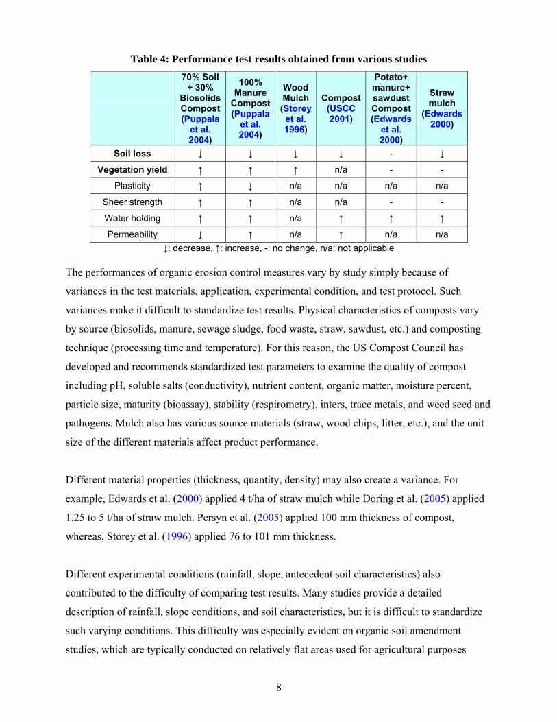
compost and mulch are effective in reducing soil loss by increasing vegetation yield (Table 4).

However, it is unclear whether their performance level is enough to be applied to steep slopes.

Moreover, the mechanism bringing about such results is not clearly addressed in the literature

supporting the effectiveness of organic amendments on erosion control and vegetation yield. The

lack of theory might limit the general application of those organic treatments.

RESUBMITTAL

8

Table 4: Performance test results obtained from various studies

70% Soil + 30%

Biosolids Compost (Puppala

et al. 2004)

100% Manure

Compost(Puppala

et al. 2004)

Wood Mulch (Storey

et al. 1996)

Compost(USCC 2001)

Potato+ manure+ sawdust Compost (Edwards

et al. 2000)

Straw mulch

(Edwards2000)

Soil loss ↓ ↓ ↓ ↓ - ↓

Vegetation yield ↑ ↑ ↑ n/a - -

Plasticity ↑ ↓ n/a n/a n/a n/a

Sheer strength ↑ ↑ n/a n/a - -

Water holding ↑ ↑ n/a ↑ ↑ ↑

Permeability ↓ ↑ n/a ↑ n/a n/a ↓: decrease, ↑: increase, -: no change, n/a: not applicable

The performances of organic erosion control measures vary by study simply because of

variances in the test materials, application, experimental condition, and test protocol. Such

variances make it difficult to standardize test results. Physical characteristics of composts vary

by source (biosolids, manure, sewage sludge, food waste, straw, sawdust, etc.) and composting

technique (processing time and temperature). For this reason, the US Compost Council has

developed and recommends standardized test parameters to examine the quality of compost

including pH, soluble salts (conductivity), nutrient content, organic matter, moisture percent,

particle size, maturity (bioassay), stability (respirometry), inters, trace metals, and weed seed and

pathogens. Mulch also has various source materials (straw, wood chips, litter, etc.), and the unit

size of the different materials affect product performance.

Different material properties (thickness, quantity, density) may also create a variance. For

example, Edwards et al. (2000) applied 4 t/ha of straw mulch while Doring et al. (2005) applied

1.25 to 5 t/ha of straw mulch. Persyn et al. (2005) applied 100 mm thickness of compost,

whereas, Storey et al. (1996) applied 76 to 101 mm thickness.

Different experimental conditions (rainfall, slope, antecedent soil characteristics) also

contributed to the difficulty of comparing test results. Many studies provide a detailed

description of rainfall, slope conditions, and soil characteristics, but it is difficult to standardize

such varying conditions. This difficulty was especially evident on organic soil amendment

studies, which are typically conducted on relatively flat areas used for agricultural purposes

RESUBMITTAL

9

rather than on steep slopes, which may alter the mechanism of erosion. It was determined that

results from studies conducted on slopes were to be used for this study since slope steepness and

length play a major role in the erosion process.

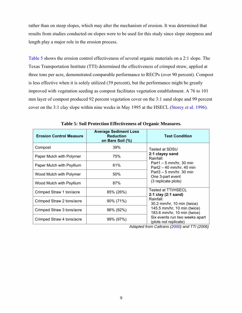
Table 5 shows the erosion control effectiveness of several organic materials on a 2:1 slope. The

Texas Transportation Institute (TTI) determined the effectiveness of crimped straw, applied at

three tons per acre, demonstrated comparable performance to RECPs (over 90 percent). Compost

is less effective when it is solely utilized (39 percent), but the performance might be greatly

improved with vegetation seeding as compost facilitates vegetation establishment. A 76 to 101

mm layer of compost produced 92 percent vegetation cover on the 3:1 sand slope and 99 percent

cover on the 3:1 clay slope within nine weeks in May 1995 at the HSECL (Storey et al. 1996).

Table 5: Soil Protection Effectiveness of Organic Measures.

Erosion Control Measure Average Sediment Loss

Reduction on Bare Soil (%)

Test Condition

Compost 39%

Paper Mulch with Polymer 75%

Paper Mulch with Psyllium 61%

Wood Mulch with Polymer 50%

Wood Mulch with Psyllium 87%

Tested at SDSU 2:1 clayey sand Rainfall: Part1 – 5 mm/hr, 30 min Part2 – 40 mm/hr, 40 min Part3 – 5 mm/hr. 30 min One 3-part event (3 replicate plots)

Crimped Straw 1 ton/acre 85% (26%)

Crimped Straw 2 tons/acre 90% (71%)



Tested at TTI/HSECL 2:1 clay (2:1 sand) Rainfall: 30.2 mm/hr, 10 min (twice) 145.5 mm/hr, 10 min (twice) 183.6 mm/hr, 10 min (twice) Six events run two weeks apart (plots not replicate)

Adapted from Caltrans (2000) and TTI (2006)

RESUBMITTAL

10

SOIL EROSION FACTORS

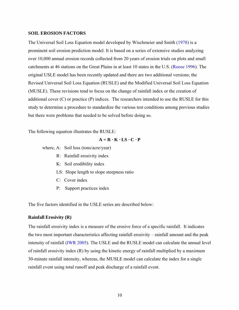
The Universal Soil Loss Equation model developed by Wischmeier and Smith (1978) is a

prominent soil erosion prediction model. It is based on a series of extensive studies analyzing

over 10,000 annual erosion records collected from 20 years of erosion trials on plots and small

catchments at 46 stations on the Great Plains in at least 10 states in the U.S. (Roose 1996). The

original USLE model has been recently updated and there are two additional versions; the

Revised Universal Soil Loss Equation (RUSLE) and the Modified Universal Soil Loss Equation

(MUSLE). These revisions tend to focus on the change of rainfall index or the creation of

additional cover (C) or practice (P) indices. The researchers intended to use the RUSLE for this

study to determine a procedure to standardize the various test conditions among previous studies

but there were problems that needed to be solved before doing so.

The following equation illustrates the RUSLE:

A = R · K · LS · C · P

where, A: Soil loss (tons/acre/year)

R: Rainfall erosivity index

K: Soil erodibility index

LS: Slope length to slope steepness ratio

C: Cover index

P: Support practices index

The five factors identified in the USLE series are described below:

Rainfall Erosivity (R)

The rainfall erosivity index is a measure of the erosive force of a specific rainfall. It indicates

the two most important characteristics affecting rainfall erosivity – rainfall amount and the peak

intensity of rainfall (IWR 2005). The USLE and the RUSLE model can calculate the annual level

of rainfall erosivity index (R) by using the kinetic energy of rainfall multiplied by a maximum

30-minute rainfall intensity, whereas, the MUSLE model can calculate the index for a single

rainfall event using total runoff and peak discharge of a rainfall event.

RESUBMITTAL

11

Soil Erodibility (K)

Soil erodibility represents the rate of runoff and the vulnerability of soil to erosion (IWR 2002).

The resistance to erosion typically depends upon the weight and coherence of soil particles. The

structure of the soil determines the amount of infiltration and runoff.

The soil erodibility index (K) used in USLE models varies from 0.7 for the most erodible soil to

0.01 for the most stable soil. The calculation for K factor is measured on bare soil plots 22.2 m

long on 9 percent slopes, tilled in the direction of the slope and having received no organic

matter for three years (Roose 1996). Wischmeier et al. (1978) conducted multiple regressions

between soil erodibility and 23 different soil parameters.

Procedure: in examining the analysis of appropriate surface samples, enter on the left of the graph and plot the percentage of silt (0.002 to 0.1 mm), then of sand (0.10 to 2 mm), then of organic matter, structure and permeability in the direction indicated by the arrows. Interpolate between the drawn curves if necessary. The broken arrowed line indicates the procedure for a sample having 65 percent silt + very fine sans, 5 percent sand, 2.8 percent organic matter, 1st approximation of K = 0.28, 2 of structure and 4 of permeability. Erodibility factor K = 0.31. Figure 1: Nomograph Allowing a Quick Assessment of the "K" Factor Of Soil Erodibility.

(Roose 1996 and reference therein; Wischmeier et. al. 1971)

% sand

% organic matter

RESUBMITTAL

12

Figure 1 demonstrates the process of the calculation of the erodibility index using major soil

characteristics including percentage of silt and very fine sand, percentage of sand, percentage of

organic matter, soil structure, and permeability. This graph indicates that lower erodibility results

from:

• lower percentage of silt and very fine sand,

• higher percentage of organic matter,

• more solid soil structure, and

• higher soil permeability.

According to the USLE, coarse textured soils like sand seem to show low erodibility due to their

weight and high infiltration/low runoff level despite their low coherence. Whereas, dense

textured soils like clay may show higher erodibility because of their lightness and high runoff

possibility despite strong coherence. As mentioned earlier, these USLE results are from tests

conducted on relatively flat 9 percent slopes. This 9 percent slope allowed infiltration rates

much higher than typical highway environments. Godfrey and Long (1994) pointed out that sand

produces high sediment yield despite its low erodibility value on slopes typically used in

highway construction (Table 6).

Table 6: Soil Erodibility Guide

Soil texture Erodibility index Sediment yield Sand 0.02 - 0.05 High

Loamy sand 0.08 - 0.12 Low

Clay 0.13 - 0.20 Low to Medium

Very fine sand 0.28 - 0.42 Medium to High

Loam 0.29 - 0.38 Medium

Silt 0.42 - 0.60 High Adapted from Godfrey et al. (1994)

Slope Steepness and Length (LS)

Increased slope steepness and length increases the potential for erosion as it increase runoff

velocity and mass. Wischmeier and Smith’ equation (1957) established such relationship (see

Figure 2). However, many studies pointed out that the equation missed the interaction between

slope and surface condition (cover type, roughness, the shape of surface line, and prior moisture)

RESUBMITTAL

13

(Roose 1996 and references therein; Roose 1973; Roose 1980a; Wischmeier 1966; and Lal

1975).

Figure 2: Relationship Among Erosion Level, And Slope Length And Steepness

(Roose 1996)

Cover (C)

Cover factor represents the effect of plants, soil cover, soil biomass, and soil disturbing activities

on erosion (IWR 2002). The cover index is the ratio of soil loss observed under a specific cover

condition to soil loss under the bare soil condition. The USLE considers only plant cover, its

production level, and the associated cropping techniques (Roose 1996). RUSLE deals with

additional cover material including various types of mulch. The index is computed with several

soil characteristics including canopy, surface cover, surface roughness, prior land use, and

antecedent soil moisture (IWR 2002). The total percent of covered area and the density of cover

material are main considerations in calculating the C factor. Cover index in the USLE varies

from 1 on bare soil to 0.001 under forest conditions.

RESUBMITTAL

14

Erosion Control Practice (P)

Various human practices to control soil surface including contour tilling, mounding, and contour

ridging can change the level of soil erosion. The support practice index provided by the USLE

varies from 1 on bare soil with no erosion control to about 0.1 with contour ridging on a gentle

slope. However, numerous experiments carried out by Asseline, Collinet, Lafforgue, Roose and

Valentin under simulated rainfall confirmed the null or negative effects of tillage on soil erosion.

In summary, Roose (1996) concluded:

• The very temporary improvement in infiltration as a result of tillage: after 120

mm of rain, there is practically no trace of this improvement on any of the soils

tested at Adiopodoumé Centre and in Burkina Faso;

• The increase in the fine suspended load in runoff after tillage;

• The extremely beneficial and lasting effect for soil and water conservation of

plant cover and of leaving crop residues on the surface; and

• The very marked but temporary effect of tied ridging and other methods aimed at

increasing the roughness of the soil (Lafforgue and Naah 1976; Roose and

Asseline 1978; Collinet and Lafforgue 1979; Collinet and Valentin 1979).

Limitations of the USLE Model

Despite the rationale based on numerous test trials in various controlled conditions, the USLE

model has intrinsic limitations as Roose (1996) concluded:

• The model applies only to sheet erosion since the source of energy is rain; so it

never applies to linear or mass erosion.

• The type of countryside: the model has been tested and verified in moderately

hilly country with 1-20 percent slopes, and excludes mountains, especially slopes

steeper than 40 percent, where runoff is a greater source of energy than rain and

where there are significant mass movements of earth.

• The relations between kinetic energy and rainfall intensity generally used in this

model apply only to the American Great Plains and not to mountainous regions

although different sub-models can be developed for the index of rainfall erosivity.

RESUBMITTAL

15

• A major limitation of the model is that it neglects certain interactions between

factors in order to distinguish more easily the individual effect of each. For

example, it does not take into account the effect on erosion of slope combined

with plant cover, nor the effect of soil type on the effect of slope.

Another limitation of the model is that it is based on gentle slopes, which do not represent the

typical steep slopes occurring along our roadsides designed and maintained by TxDOT. The test

slopes at the HSECL are 33 percent and 50 percent, which more accurately reflect ‘real-world’

conditions.

RESUBMITTAL

RESUBMITTAL

17

METHODOLOGY

DATA COLLECTION AND TREATMENT

Cost of Products on the Approved Product List

A telephone survey was used to collect product cost data. The information includes product price

per 10,000 square yards, installation cost, product size, and discount availability (if any). During

the survey, the researchers also identified discontinued products and products manufactured

under multiple trade names on the TxDOT APL (Appendix C). The APL includes 60 slope

protection products and 47 channel protection products after excluding discontinued or

duplicated products. Among all of these products, 16 products have been approved for use on

both slope and channel protection.

During the telephone survey, many manufacturers were reluctant to provide price information as

they recognized the survey was part of a comparison study. The price survey obtained about 80

percent and 65 percent of response rate for slope products and channel products, respectively

(Table 7). Installation costs were difficult to obtain since labor costs vary by region. It was

expected that end-users (such as municipalities and governmental bodies) could provide the

approximate installation cost by product type (i.e., mulch, composite, synthetic, etc.) but such

detailed information was not available. TxDOT provides bid price information; however, this

information is not based on product type but by specific project condition including soil type and

slope steepness or channel shear stress. Hence, the researcher’s utilized only material price

collected from the telephone survey for the cost-performance analysis.

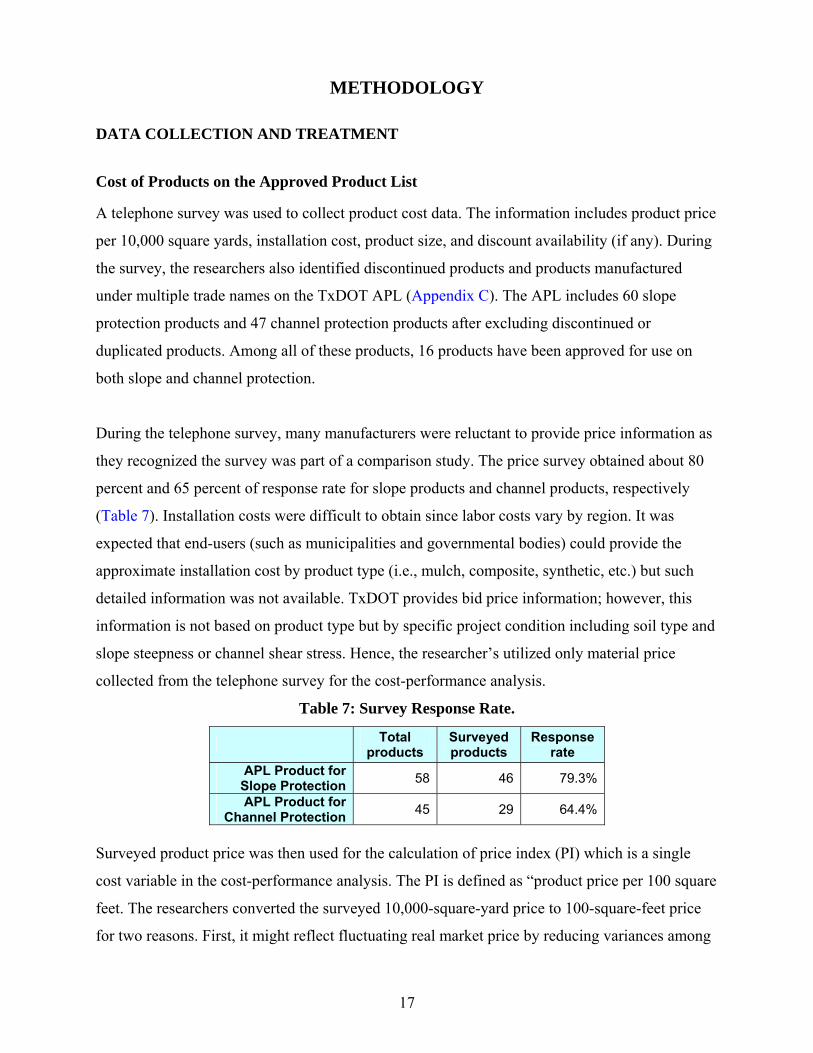
Table 7: Survey Response Rate.

Total products

Surveyed products

Response rate

APL Product for Slope Protection 58 46 79.3%

APL Product for Channel Protection 45 29 64.4%

Surveyed product price was then used for the calculation of price index (PI) which is a single

cost variable in the cost-performance analysis. The PI is defined as “product price per 100 square

feet. The researchers converted the surveyed 10,000-square-yard price to 100-square-feet price

for two reasons. First, it might reflect fluctuating real market price by reducing variances among

RESUBMITTAL

18

price data (i.e., ‘$ 3200’ to ‘$ 4000’ has same index value ‘4’). Second, the unit area of 100

square feet matches the criteria TxDOT uses in quantifying the soil loss performance, that is,

pounds per 100 square feet. Unit matching is important when calculating the cost-benefit ratio.

The price index is expressed by:

Price Index (PI) = Price per 100 ft2 = Price per 10,000 yd2 / 900

Soil Loss Data

Soil loss performance data of the TxDOT APL originates from experiments conducted at the TTI

HSECL. The HSECL evaluates slope protection products in four soil-slope conditions including

clay and sand in 1V:2H slope, and clay and sand in 1V:3H slope, and channel protection

products in six shear stress conditions (i.e., 0 to 2, 0 to 4, 0 to 6, 0 to 8, 0 to 10, and 0 to 12

lb/ft2). This testing program began in 1991 and changed its protocol from outdoor field testing to

large-scale indoor testing in 2000. TxDOT (2000) and TxDOT (2005) detail the outdoor and

indoor experimental protocols, respectively. To investigate the influence by difference of test

protocol on the indoor vs. outdoor data, Li et al. (2003) conducted a comparison study on data

collected from the two different test protocols. They found that the ratio between field and indoor

data in HSECL slope erosion experiments is relatively constant regardless of soil type and test

slope (Table 8). Therefore, the researchers use the average value ‘0.088’ to standardize the APL

slope soil loss data.

Table 8: Ratio of Field Soil Loss Data to Indoor Soil Loss Data of The HSECL.

(adapted from Li et al. 2003)

Product Type Field Soil Loss

(kg/10m2) Indoor Soil Loss

(kg/10m2) Soil Loss Ratio 1:2 Clay

Product A 0.18 2.05 0.088 Product B 0.24 3.75 0.064 Product C 0.19 3.06 0.062 Product D 0.31 2.22 0.140

Average 0.089

1:2 Sand Product A 23.42 306.60 0.076 Product B 18.81 279.86 0.067 Product C 21.85 181.79 0.120 Product D 26.47 312.57 0.085

Average 0.087

RESUBMITTAL

19

Table 8: Ratio of Field Soil Loss Data to Indoor Soil Loss Data of the HSECL. (cont)_

Product Type Field Soil Loss

(kg/10m2) Indoor Soil Loss

(kg/10m2) Soil Loss Ratio 1:3 Clay

Product C 0.15 1.62 0.093 Product D 0.27 2.11 0.127 Product E 0.15 2.82 0.053 Product F 0.31 4.02 0.078

Average 0.088

1:3 Sand Product C 8.00 82.94 0.096 Product D 8.12 72.61 0.112 Product E 4.42 57.60 0.077 Product F 11.95 170.29 0.070

Average 0.089

• Product A – turf reinforcement mat (TRM) made of polypropylene fibers bound together by two biaxially oriented nets and stitched with polypropylene thread, manufactured by Synthetic Industries.

• Product B – open weave textile (OWT) made of polypropylene fibers woven together, manufactured by Synthetic Industries.

• Product C – erosion control blanket (ECB) made of wheat straw bound together by top and bottom jute netting and stitched with twisted jute thread, manufactured by Synthetic Industries.

• Product D – ECB made of straw fibers bound together by top polypropylene netting sewn together by degradable thread, manufactured by North American Green.

• Product E – ECB made of aspen curled wood excelsior bound together by top degradable netting, manufactured by American Excelsior Company.

• Product F – bonded fiber matrix (BFM) consisting of long strand, residual, softwood fibers joined together by adhesive, manufactured by Canfor.

Such a comparison study described above is not necessary for channel test data since the tests

were all conducted on a vegetated surface in both old and new protocols. The soil loss value for

channel products indicates the change of surface elevation after a series of flume tests with

different shear stresses. Both field and flume test protocols recorded soil loss depth in inches.

To develop the soil loss index (SLI) that could represent a products’ soil loss level, researchers

classified the soil loss test data of the HSECL. To classify soil loss data in both channel and

slope protection products, the researchers use the APL maximum allowable sediment loss

thresholds. The researchers defined that if the soil loss of a product is within 0 to 10 percent of

RESUBMITTAL

20

the threshold, the SLI value is ‘5’ which indicates the best product. Likewise, 10.1 to 20 percent

of the threshold has a value of ‘15’, and 90.1 to 100 percent has a value of ‘95’ which represents

the lowest performing group among products in the APL. A product that failed on the APL test

has a value of over 100 (%).

Tables 9 and 10 show the performance thresholds for the slope and channel tests, respectively.

The thresholds have been determined from a series of statistical tests on over 100 products for 6

years (Northcutt and McFalls 1997).

Table 9: Threshold Of TxDOT APL Slope Test.

Slope & Soil Soil Loss (lb/100 ft2)

1:3 Clay 7.891:2 Clay 7.891:3 Sand 284.301:2 Sand 631.80

Table 10: Threshold Of TxDOT APL Channel Test

Soil Loss Shear Stress

Range (lb/ft2) (lb/100 ft2) (in) 0 - 2 350 0.43 0 - 4 500 0.48 0 - 6 620 0.60 0 - 8 800 0.77

0 - 10 1180 1.13 0 - 12 1200 1.15

The purposes of using the SLI rather than the actual soil loss value are as follows:

• The problem associated with data variance could be alleviated due to the variance that

might result from minor experiment errors. For example, the value of 5 is assigned to

cover soil loss ranges from 0 to 63.18 lb/100 ft2 in 1:2 sand slopes (Table 11).

• The test protocol assumes that a product can protect conditions that are less severe than

the level for which it is approved. For example, a product approved for 1:2 slopes on clay

also qualifies for 1:3 slopes on clay. In this case, the researchers assume the product has

the same soil protection performance in both 1:2 and 1:3 slopes on clay.

RESUBMITTAL

21

Tables 11 and 12 show the assumed soil loss index that corresponds to soil loss ranges in pounds

per 100 square feet. The researchers used the soil loss index, along with the longevity of a

product, as the performance variable of a product.

Table 11: Soil Loss Index and Corresponding Soil Loss Range for Slope Protection

Products.

Soil Loss (lb/100 ft2) Criteria

Soil Loss Index

(% to APL threshold) 1:3 Clay 1:2 Clay 1:3 Sand 1:2 Sand

0~10% of threshold 5 0.00~0.79 0.00~0.79 0.00~28.43 0.00~63.18

10~20% of threshold 15 0.80~1.58 0.80~1.58 28.44~56.86 63.19~126.36

20~30% of threshold 25 1.59~2.37 1.59~2.37 56.87~85.29 126.37~189.54

30~40% of threshold 35 2.38~3.16 2.38~3.16 85.30~113.72 189.55~252.72

40~50% of threshold 45 3.17~3.95 3.17~3.95 113.73~142.15 252.73~315.90

50~60% of threshold 55 3.96~4.73 3.96~4.73 142.16~170.58 315.91~379.08

60~70% of threshold 65 4.74~5.52 4.74~5.52 170.59~199.01 379.09~442.26

70~80% of threshold 75 5.53~6.31 5.53~6.31 199.02~227.44 442.27~505.44

80~90% of threshold 85 6.32~7.10 6.32~7.10 227.45~255.87 505.45~568.62

90~100% of threshold 95 7.11~7.89 7.11~7.89 255.88~284.30 568.63~631.80

Table 12: Soil Loss Index and Corresponding Soil Loss Range for Channel Protection

Products

Soil Loss (in) Criteria

Soil loss Index

(% to APL threshold) 0 - 2 0 - 4 0 - 6 0 - 8 0 - 10 0 - 12

0~10% of threshold 5 0.00~0.04 0.00~0.05 0.00~0.06 0.00~0.08 0.00~0.11 0.00~0.12

10~20% of threshold 15 0.05~0.09 0.06~0.10 0.07~0.12 0.09~0.15 0.12~0.23 0.13~0.23

20~30% of threshold 25 0.10~0.13 0.11~0.14 0.13~0.18 0.16~0.23 0.23~0.34 0.24~0.35

30~40% of threshold 35 0.14~0.17 0.15~0.19 0.19~0.24 0.24~0.31 0.35~0.45 0.36~0.46

40~50% of threshold 45 0.18~0.22 0.20~0.24 0.25~0.30 0.32~0.38 0.46~0.57 0.47~0.58

RESUBMITTAL

22

50~60% of threshold 55 0.23~0.26 0.25~0.29 0.31~0.36 0.39~0.46 0.58~0.68 0.59~0.69

60~70% of threshold 65 0.27~0.30 0.30~0.34 0.37~0.42 0.47~0.54 0.69~0.79 0.70~0.81

70~80% of threshold 75 0.31~0.34 0.35~0.38 0.43~0.48 0.55~0.61 0.80~0.91 0.82~0.92

80~90% of threshold 85 0.35~0.39 0.39~0.43 0.49~0.54 0.62~0.69 0.92~1.02 0.93~1.04

90~100% of threshold 95 0.40~0.43 0.44~0.48 0.55~0.60 0.70~0.77 1.03~1.13 1.05~1.15

Product Type (Classified by Material Composition and Longevity)

This study classifies material composition into four types – 1) mulch, 2) natural, 3) composite,

and 4) synthetic. The mulch category represents spray-on products while the other three

categories represent RECPs. The natural type specifies products composed of natural fill

materials including jute, coconut fibers and excelsior with a bio-degradable netting. Composite

products are generally composed of natural materials and non-biodegradable synthetic netting.

The material composition is an important factor determining the longevity and environmental

friendliness of an erosion control product. For example, synthetic products tend to perform better

and have a longer lifetime than natural products, while natural ones are more environmentally

compatible than synthetic products. Most composite products tend to be fill in the gap between

the pure-natural or pure-synthetic products.

Longevity is an important factor affecting soil protection performance because longer lifetime

provides longer protection. The researchers define five categories of longevity as follows.

• temporary term (0 - 3 months);

• short term (3 -12 months);

• mid term (12 - 24 months);

• long term (24 - 36 months); and

• permanent term (over 36 months and up to 54 months ).

The researchers classify all products in the APL into ten categories based on material

composition and longevity in the following list.

• Temporary Mulch (TM): These products are hydraulically applied using spray-on

procedures. Temporary mulches can be mixed with seed to establish both temporary

erosion control and seeding in the same application. The types of temporary mulches vary

RESUBMITTAL

23

greatly from simple low slope products to complex BFMs and mulches that are designed

for severe slope applications. Temporary mulches are design for ease of application and

to aid in rapid vegetative establishment in a variety of settings.

• Temporary Natural (TN): Products in this category are temporary all-natural blankets.

The netting, stitching, and fill material of these blankets is made up entirely of natural

materials. These blankets are ultra-short term in use and are designed to degrade quickly

and last only until vegetation can be established.

• Temporary Composite (TC): Products in this category are temporary blankets that

contain natural filler material and synthetic netting and/or stitching. These blankets can

be either single or double net products with a netting that photodegrades or biodegrades

very quickly. These blankets are designed for temporary erosion control until vegetation

can be established.

• Short-term Natural (SN): Products in this category are short-term all-natural blankets.

The netting, stitching, and fill material of these blankets is made up entirely of natural

materials. These blankets are short term in use and are designed to degrade rapidly. These

blankets last longer than temporary products and can assist in protecting the soil until

more dense vegetation is established.

• Short-term Composite (SC): Products in this category are short-term blankets that contain

natural filler material and synthetic netting and/or stitching. These blankets can be either

single or double net products with a netting that photodegrades or biodegrades quickly.

These blankets are designed for short term erosion control and last long enough to

provide that adequate vegetation can be successfully established.

• Mid-term Natural (MN): Products in this category are mid-term all-natural blankets. The

netting, stitching, and fill material of these blankets is made up entirely of natural

materials. These blankets provide erosion control until vegetation can be established and

remain for some time after vegetation is growing to help continue to provide erosion

control in conjunction with the vegetation. These products are usually double net

products.

• Mid-term composite (MC): Products in this category are mid-term blankets that contain

natural filler material and synthetic netting and/or stitching. These blankets are usually

always double net products with a medium strength synthetic netting that photodegrades

RESUBMITTAL

24

or biodegrades slowly. These blankets are designed to last until vegetation is fully

established and can protect the soil.

• Long-term Natural (LN): Products in this category are long-term all-natural blankets. The

netting, stitching and fill material of these blankets is made up entirely of long-lasting

natural materials. These blankets provide erosion control until vegetation can be

established and remain long after vegetation is growing to help continue to provide

erosion control and establish a good root system and dense coverage in the vegetation.

These products are designed to last until total revegetation and permanent vegetative

establishment has been achieved.

• Long-term Composite (LC): Products in this category are long-term blankets that contain

natural filler material and synthetic netting and/or stitching. These blankets are usually

always double net products with a strong synthetic netting that photodegrades or

biodegrades very slowly. These blankets are designed for long-term erosion control and

to provide total vegetative establishment and strong root system establishment. These

blankets also remain long after vegetation is growing to help continue to provide erosion

control.

• Permanent Synthetic (PS): These products are totally synthetic blankets, which usually

contain a stable polypropylene or similar synthetic fiber and netting. These blankets are

designed for permanent erosion control protection and are designed to be used in

situations where vegetation alone is not adequate and permanent continuing erosion

control is needed. These blankets are designed to work with vegetation permanently to

provide protection for severe erosion control applications.

Table 13 shows the classification of product type based on material type and longevity.

Table 13: Classification of Product Type.

Material composition Mulch Natural Composite Synthetic Environmental Friendliness Good Good Fair Poor

Temporary 3 mo TM TN TC . Short 12 mo . SN SC . Mid 24 mo . MN MC . Long 36 mo . LN LC .

Longevity

Permanent 54 mo . . . PS

RESUBMITTAL

25

LIFETIME SOIL PROTECTION PERFORMANCE

APL soil loss test data and corresponding soil loss index (SLI) indicate initial performance rather

than lifetime performance. This section introduces the concept of lifetime soil protection

performance that reflects the change of the performance over a product’s lifetime.

Lifetime Soil Protection by Product

Assumptions for estimating soil amount protected by products include:

• Soil protection performance of a product decreases with time. Specific details include:

o Performance of a product decreases linearly over time;

o Soil loss data obtained from HSECL’s testing represents the initial soil loss level

of products.

o The soil loss of a product at the end of its lifespan is set as 150 percent of the APL

threshold (i.e., 150 percent of the soil loss index) when the product no longer

protects the soil.

o The condition is considered failed, when the soil loss level exceeds 150 percent of the threshold.

Figure 3 shows an example of soil protection ability of various products over time. In this

example, a product with temporary longevity (3 months) loses the highest amount of soil during

the initial period, while a product with permanent longevity (54 months) loses the least amount

of soil. Also for comparison purposes, the soil loss produced by all products at the end of their

lifespan is set the same as 150 percent of the APL threshold.

RESUBMITTAL

26

0

50

100

150

200

0 6 12 18 24 30 36 42 48 54

Time (months)

Soil

Loss

(%)

% o

f soi

l los

s to

TTI

thre

shol

d

Temp Short Mid Permanent

Figure 3: An Example of Life-Performance Of Erosion Control Products.

The life-long performance line of a product can be expressed as:

Soil Loss product, time =

Final Soil Loss product – Initial Soil Loss product

Product Longevity · Time + Initial Soil Loss product

where,

Soil Loss product, time = Soil loss level of a product at a specific time (% of soil loss to APL threshold)

Final Soil Loss product = Soil loss level when the product no longer protects the soil. It is set as ‘150’ (% of soil loss to APL threshold)

Initial Soil Loss product = Soil loss level immediately after the product is installed. It is extracted from HSECL’s soil loss data (% of soil loss to APL threshold)

Product Longevity = Longevity of the product (months)

Time = A specific time (months)

Lifetime Soil Protection by Vegetation

Assumptions for estimating soil amount protected by vegetation include:

• Vegetation’s ability to protect soil increases over time. Specific details include:

RESUBMITTAL

27

o Vegetation’s ability to protect increases linearly with time.

o The initial soil loss level of vegetation starts at 150 percent of the APL threshold

when no vegetation has established.

o The final soil loss of well-established, mature vegetation is set at 4 percent of the

APL threshold. The 4 percent value is considered for the natural erosion

condition. The 4 percent value also avoids infinite value in calculating the CPI

when a product starts at 5 percent with a longevity rate the same as the vegetation

establishment time.

Vegetation’s initial soil loss level is set at 150 percent of the APL threshold because no

vegetation is assumed at the initial stage of seeding. The soil protection performance of

vegetation increases with time assuming vegetation steadily grows. Hence, the soil loss level

decreases with time and is finally set at 4 percent of the APL threshold when the vegetation is

fully established. The time required for complete vegetation establishment depends on the

conditions of a project such as slope steepness, climate, and soil type. Figure 4 shows an

example of the soil protection ability of vegetation with different establishment times

(temporary, short, etc.).

0

50

100

150

200

0 6 12 18 24 30 36 42 48 54

Time (months)

Soil

Loss

(%)

% o

f soi

l los

s to

TTI

thre

shol

d

Temp Short Mid Permanent

Figure 4: An Example of Vegetation Performance with Different Establishing Times.

RESUBMITTAL

28

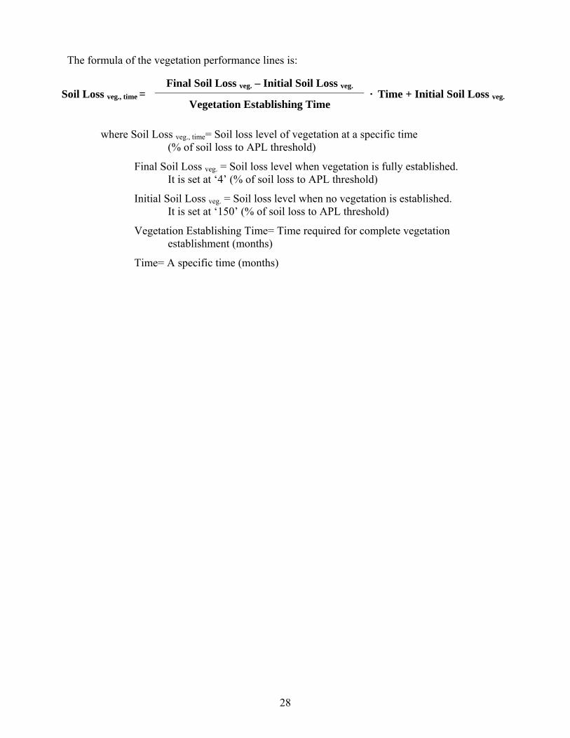
The formula of the vegetation performance lines is:

Final Soil Loss veg. – Initial Soil Loss veg. Soil Loss veg., time =

Vegetation Establishing Time · Time + Initial Soil Loss veg.

where Soil Loss veg., time= Soil loss level of vegetation at a specific time (% of soil loss to APL threshold)

Final Soil Loss veg. = Soil loss level when vegetation is fully established. It is set at ‘4’ (% of soil loss to APL threshold)

Initial Soil Loss veg. = Soil loss level when no vegetation is established. It is set at ‘150’ (% of soil loss to APL threshold)

Vegetation Establishing Time= Time required for complete vegetation establishment (months)

Time= A specific time (months)

RESUBMITTAL

29

COST-PERFORMANCE INDEX

Basic Concept

The Cost-Performance Index (CPI) was developed to quantify the cost effectiveness of erosion

control products during a designated period. The CPI considers 1) cost, 2) initial soil protection

performance, and 3) longevity. As mentioned earlier, this study uses product prices surveyed

from manufacturers as cost, and test results of the HSECL as initial performance. The product

longevity was determined based on material composition.

The CPI is defined as the potential soil protection benefit per the cost of both product and

potential topsoil replacement expense. The CPI can be expressed as:

Benefit of Potential Soil Protection CPI =

Product Expense + Cost of Potential Topsoil Loss

Thus, a higher CPI means better cost-effectiveness of a product. An important step of the CPI

development is to estimate potential protected soil amount and potential soil loss amount. For the

slope protection, the estimation of the soil amounts includes the amount protected by products

and the amount protected by vegetation. For channel protection, only the amount protected by

products is considered because HSECL’s channel APL tests are conducted on vegetated

conditions.

Cost-Performance Index for Slope Products

The estimate of slope product performance considers both product and vegetation performance.

Figure 5 shows the example that combines mid-product (24 months) and 12-month maturing

time for vegetation. The resulting trend line in this example is shown as the bold line in Figure 5.

This trend line indicates the combined performance of products and vegetation over time.

RESUBMITTAL

30

0

50

100

150

200

0 6 12 18 24

Time (months)

Soil

Loss

(%)

% o

f soi

l los

s to

TTI

thre

shol

d

Product Vegetation Combined

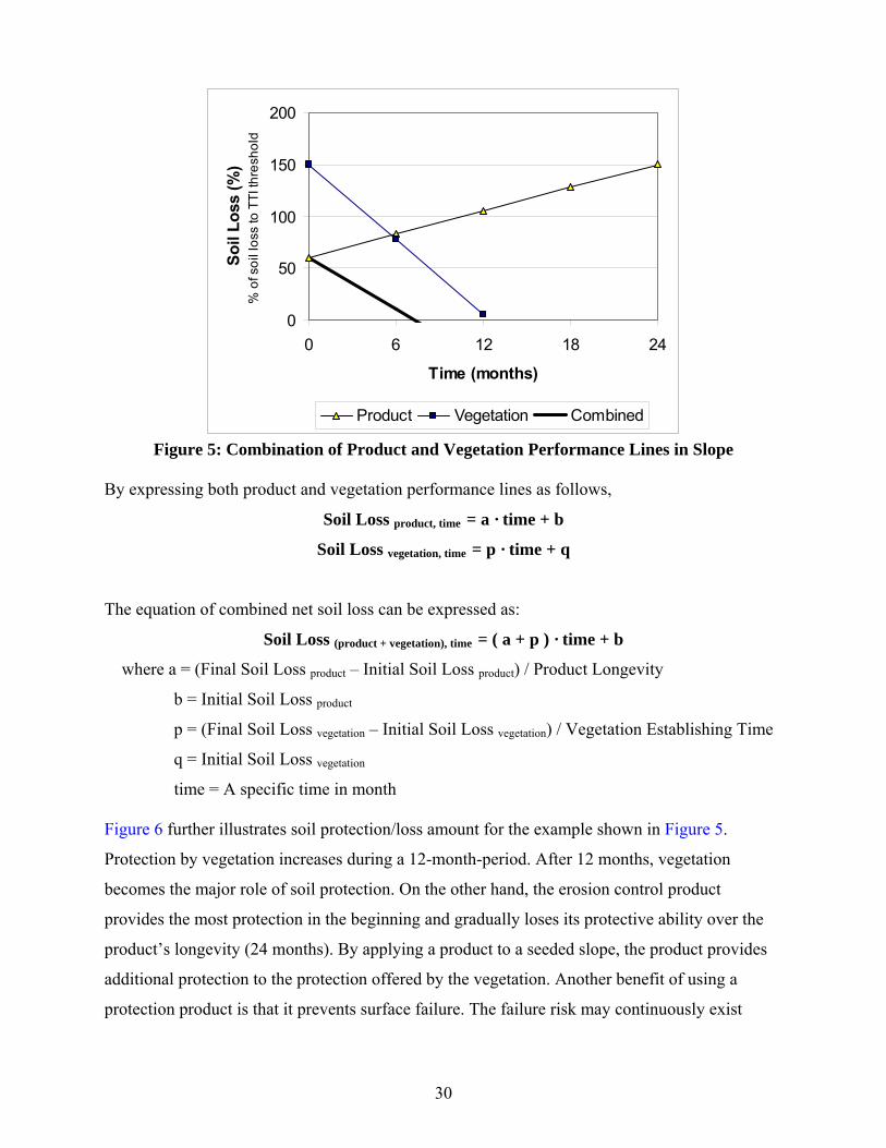
Figure 5: Combination of Product and Vegetation Performance Lines in Slope By expressing both product and vegetation performance lines as follows,

Soil Loss product, time = a · time + b

Soil Loss vegetation, time = p · time + q

The equation of combined net soil loss can be expressed as:

Soil Loss (product + vegetation), time = ( a + p ) · time + b

where a = (Final Soil Loss product – Initial Soil Loss product) / Product Longevity

b = Initial Soil Loss product

p = (Final Soil Loss vegetation – Initial Soil Loss vegetation) / Vegetation Establishing Time

q = Initial Soil Loss vegetation

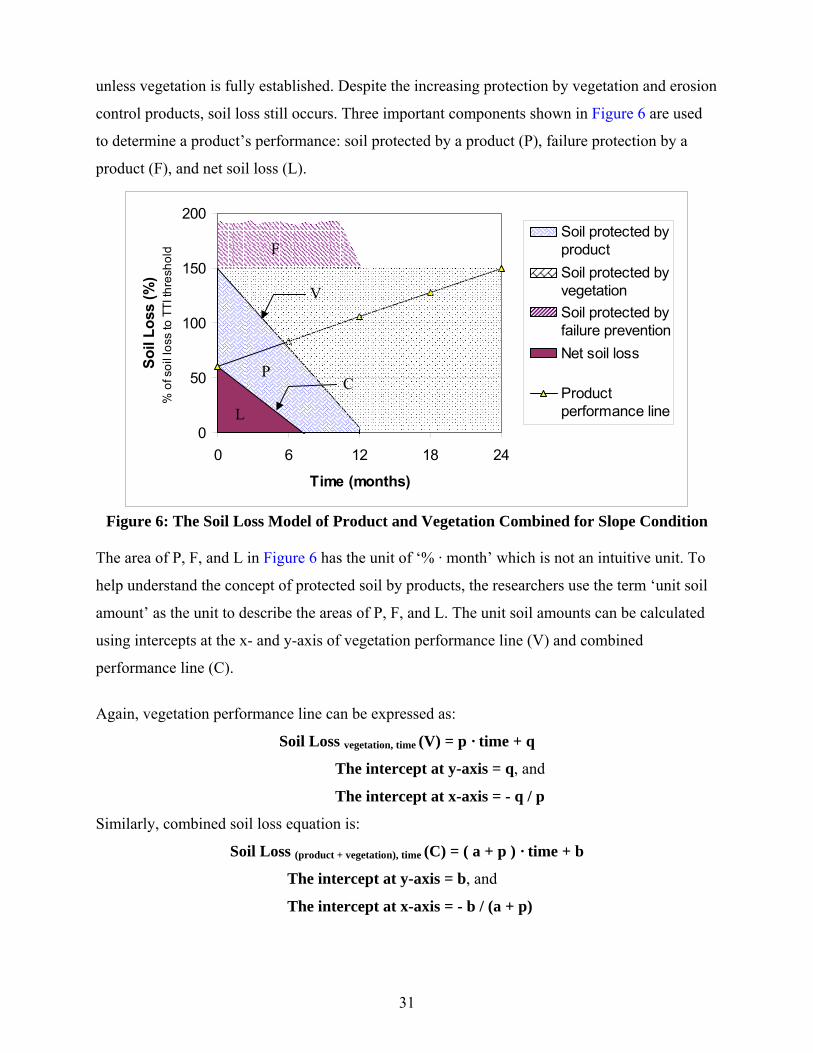
time = A specific time in month Figure 6 further illustrates soil protection/loss amount for the example shown in Figure 5.

Protection by vegetation increases during a 12-month-period. After 12 months, vegetation

becomes the major role of soil protection. On the other hand, the erosion control product

provides the most protection in the beginning and gradually loses its protective ability over the

product’s longevity (24 months). By applying a product to a seeded slope, the product provides

additional protection to the protection offered by the vegetation. Another benefit of using a

protection product is that it prevents surface failure. The failure risk may continuously exist

RESUBMITTAL

31

unless vegetation is fully established. Despite the increasing protection by vegetation and erosion

control products, soil loss still occurs. Three important components shown in Figure 6 are used

to determine a product’s performance: soil protected by a product (P), failure protection by a

product (F), and net soil loss (L).

Figure 6: The Soil Loss Model of Product and Vegetation Combined for Slope Condition

The area of P, F, and L in Figure 6 has the unit of ‘% · month’ which is not an intuitive unit. To

help understand the concept of protected soil by products, the researchers use the term ‘unit soil

amount’ as the unit to describe the areas of P, F, and L. The unit soil amounts can be calculated

using intercepts at the x- and y-axis of vegetation performance line (V) and combined

performance line (C).

Again, vegetation performance line can be expressed as:

Soil Loss vegetation, time (V) = p · time + q

The intercept at y-axis = q, and

The intercept at x-axis = - q / p

Similarly, combined soil loss equation is:

Soil Loss (product + vegetation), time (C) = ( a + p ) · time + b

The intercept at y-axis = b, and

The intercept at x-axis = - b / (a + p)

0

50

100

150

200

0 6 12 18 24

Time (months)

Soil

Loss

(%)

% o

f soi

l los

s to

TTI

thre

shol

d

Soil protected byproductSoil protected byvegetationSoil protected byfailure preventionNet soil loss

Productperformance lineL

F

V

P

C

RESUBMITTAL

32

Using the intercepts from vegetation and combined performance lines (V and C), the area of unit

net soil loss (L) and unit soil protected by product (P) can be calculated as follows:

Unit Net Soil Loss (L) = b · (- b / (a + p)) / 2

Unit Soil Protected product (P) = q · (q / p) / 2 – Unit Net Soil Loss (L)



p = (Final Soil Loss vegetation – Initial Soil Loss vegetation) / Vegetation Establishing Time

q = Initial Soil Loss vegetation

time = A specific time in month

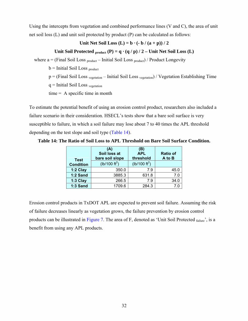
To estimate the potential benefit of using an erosion control product, researchers also included a

failure scenario in their consideration. HSECL’s tests show that a bare soil surface is very

susceptible to failure, in which a soil failure may lose about 7 to 40 times the APL threshold

depending on the test slope and soil type (Table 14).

Table 14: The Ratio of Soil Loss to APL Threshold on Bare Soil Surface Condition. (A)

Soil loss at bare soil slope

(B) APL

threshold Ratio of A to B Test

Condition (lb/100 ft2) (lb/100 ft2) 1:2 Clay 350.0 7.9 45.0

1:2 Sand 3885.3 631.8 7.0 1:3 Clay 266.5 7.9 34.0

1:3 Sand 1709.6 284.3 7.0 Erosion control products in TxDOT APL are expected to prevent soil failure. Assuming the risk

of failure decreases linearly as vegetation grows, the failure prevention by erosion control

products can be illustrated in Figure 7. The area of F, denoted as ‘Unit Soil Protected failure’, is a

benefit from using any APL products.

RESUBMITTAL

33

0

150

300

450

600

750

0 6 12 18 24

Time (months)

Soil

Loss

(%)

% o

f soi

l los

s to

TTI

thre

shol

d

Soil protected byproductSoil protected byvegetationSoil protected byfailure preventionNet soil loss

Productperformance line

Figure 7: Failure Prevention by Erosion Control Product (F).

The unit amount of soil protected by failure prevention can be calculated by:

Unit Soil Protected failure (F) = (Soil Loss bare – Final Soil Loss product) * time / 2

where Unit Soil Protected failure = Unit soil amount protected by failure prevention

Soil Loss bare = Soil loss level of bare soil condition (% of soil loss to APL threshold).

Final Soil Loss product = Soil loss level when the product no longer protects the soil.

It is set as ‘150’ (% of soil loss to APL threshold) To compare benefits and costs, this study translates the unit soil amount to dollar value per 100

square feet of slope surface. Such adjustment was conducted in two steps: (1) estimate soil

amount from ‘unit soil amount’; and (2) translate the soil amount to monetary value. The unit of

‘unit soil amount’ is ‘percent of soil loss to the APL threshold’ times month (% · month). With

the assumption that rainfall occurs once a month with the same intensity as HSECL’s test

condition, the unit soil amount multiplied by the APL threshold yields the amount of soil in

lb/100 ft2. This study makes the assumption that the actual rainfall frequency and intensity varies

by location and season. Nevertheless, the HSECL’s rainfall standard is considered severe enough

to determine better performing products because the rainfall intensity used by the HSECL

(3.5 in/hr) is much higher than most rainfall events in the state of Texas. According to TxDOT’s

F

RESUBMITTAL

34

latest hydrology research, the 99th percentile rainfall intensity in Brazos County, where HSECL

is located, is 2.08 in/hr. The soil amount is calculated by:

Soil amount (lb/100 ft2· month) = Unit soil amount (% · month) · APL threshold (lb/100 ft2) / 100 (%)

The value of soil in dollars per square feet is obtained by multiplying the soil amount by topsoil

price per pound expressed as:

Value of soil ($/100 ft2· month) = Soil Amount (lb/100 ft2· month) · Topsoil Price ($/lb)

Topsoil price varies by location. Given the limitation of information, the researchers used a

topsoil price, $25/yd3, equivalent to 0.01 $/lb considering the soil density of 1.4 g/cm3. The

calculation is as follows:

Topsoil Price = 25 ($/yd3) / 1.4 (g/cm3) = 0.92 ($/ft3) / 88 (lb/ft3) = 0.01 ($/lb) Using this soil value, the researchers can identify potential benefit and cost when using any

erosion control product. The CPI is defined as the potential soil protection benefit per the cost of

both product and potential topsoil loss. The benefit is the value of soil amount protected by

using an erosion control product, which includes basic failure protection and additional soil

protection. The cost includes the cost of the product as the well as the value of soil loss that

needs repair using topsoil.

Benefit of Potential Soil Protection CPI =

Product Expense + Cost of Potential Topsoil Loss

Value of Soil Protected ($/100 ft2) =

Product Cost ($/100 ft2) + Value of Net Soil Loss ($/100 ft2) where, Value of Soil Protected =

(Unit Soil Protected failure (F) + Unit Soil Protected product (P))

100 · APL threshold · Topsoil price

Product Cost = Product price from telephone survey

Value of soil loss = Unit Net Soil Loss (L) / 100 · APL threshold · Topsoil price

RESUBMITTAL

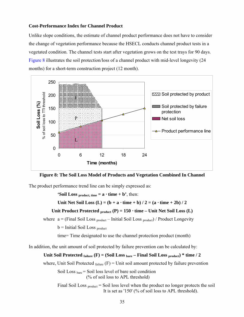
35

Cost-Performance Index for Channel Product

Unlike slope conditions, the estimate of channel product performance does not have to consider

the change of vegetation performance because the HSECL conducts channel product tests in a

vegetated condition. The channel tests start after vegetation grows on the test trays for 90 days.

Figure 8 illustrates the soil protection/loss of a channel product with mid-level longevity (24

months) for a short-term construction project (12 month).

0

50

100

150

200

250

0 6 12 18 24

Time (months)

Soil

Loss

(%)

% o

f soi

l los

s to

TTI

thre

shol

d Soil protected by product

Soil protected by failureprotectionNet soil loss

Product performance line

Figure 8: The Soil Loss Model of Products and Vegetation Combined In Channel

The product performance trend line can be simply expressed as:

‘Soil Loss product, time = a · time + b’, then:

Unit Net Soil Loss (L) = (b + a · time + b) / 2 = (a · time + 2b) / 2

Unit Product Protected product (P) = 150 · time – Unit Net Soil Loss (L)



time= Time designated to use the channel protection product (month) In addition, the unit amount of soil protected by failure prevention can be calculated by:

Unit Soil Protected failure (F) = (Soil Loss bare – Final Soil Loss product) * time / 2

where, Unit Soil Protected failure (F) = Unit soil amount protected by failure prevention

Soil Loss bare = Soil loss level of bare soil condition (% of soil loss to APL threshold)

Final Soil Loss product = Soil loss level when the product no longer protects the soil

F

P

L

RESUBMITTAL

It is set as '150' (% of soil loss to APL threshold).

36

It is set as ‘150’ (% of soil loss to APL threshold).

After translating the unit soil amounts explained above to monetary values, the cost-performance

index for a channel product can be calculated by:

Value of Soil Protected ($/100 ft2) CPI =

Product cost ($/100 ft2) + Value of Soil Loss ($/100 ft2) where Value of Soil Protected =

(Unit Soil Protected failure (F) + Unit Soil Protected product (P))

100 · APL threshold · Topsoil price

Product Cost = Product price from telephone survey

Value of soil loss = Unit Net Soil Loss (L) / 100 · APL threshold · Topsoil price

RESUBMITTAL

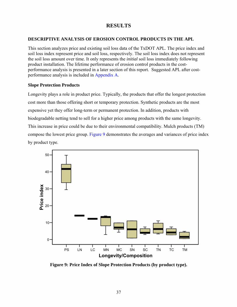
37

RESULTS

DESCRIPTIVE ANALYSIS OF EROSION CONTROL PRODUCTS IN THE APL

This section analyzes price and existing soil loss data of the TxDOT APL. The price index and soil loss index represent price and soil loss, respectively. The soil loss index does not represent the soil loss amount over time. It only represents the initial soil loss immediately following product installation. The lifetime performance of erosion control products in the cost-performance analysis is presented in a later section of this report. Suggested APL after cost-performance analysis is included in Appendix A.

Slope Protection Products

Longevity plays a role in product price. Typically, the products that offer the longest protection

cost more than those offering short or temporary protection. Synthetic products are the most

expensive yet they offer long-term or permanent protection. In addition, products with

biodegradable netting tend to sell for a higher price among products with the same longevity.

This increase in price could be due to their environmental compatibility. Mulch products (TM)

compose the lowest price group. Figure 9 demonstrates the averages and variances of price index

by product type.

PS LN LC MN MC SN SC TN TC TM

Longevity/Composition

0

10

20

30

40

50

Pric

e in

dex

Figure 9: Price Index of Slope Protection Products (by product type).

RESUBMITTAL

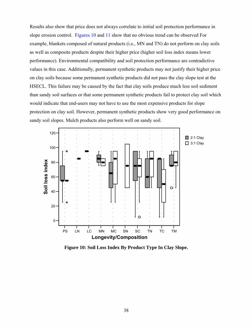
38

Results also show that price does not always correlate to initial soil protection performance in

slope erosion control. Figures 10 and 11 show that no obvious trend can be observed For

example, blankets composed of natural products (i.e., MN and TN) do not perform on clay soils

as well as composite products despite their higher price (higher soil loss index means lower

performance). Environmental compatibility and soil protection performance are contradictive

values in this case. Additionally, permanent synthetic products may not justify their higher price

on clay soils because some permanent synthetic products did not pass the clay slope test at the

HSECL. This failure may be caused by the fact that clay soils produce much less soil sediment

than sandy soil surfaces or that some permanent synthetic products fail to protect clay soil which

would indicate that end-users may not have to use the most expensive products for slope

protection on clay soil. However, permanent synthetic products show very good performance on

sandy soil slopes. Mulch products also perform well on sandy soil.

PS LN LC MN MC SN SC TN TC TM


0

20

40

60

80

100

120

Soil

loss

inde

x

2:1 Clay3:1 Clay

Figure 10: Soil Loss Index By Product Type In Clay Slope.

RESUBMITTAL

39

PS LC MN MC SN SC TN TC TM


0

20

40

60

80

100

120

140

Soil

loss

inde

x

2:1 Sand3:1 Sand

Figure 11: Soil Loss Index By Product Type In Sand Slope

Channel Protection Products

Channel protection products are required to be more durable and last longer than slope products

since they must protect vegetation from concentrated channel flow rather than sheet flow. As

mentioned earlier, prices are affected by longevity but research indicates there is a small

difference in price especially between permanent products (i.e., PS: over 3 years) and long-term

products (i.e., LN and LC: 2 to 3 years). The use of natural materials does not affect the price of

channel protection products which indicates that performance is the primary factor (over

environmental compatibility) for channel protection. Figure 12 shows the price trend by product

type.

RESUBMITTAL

40

PS LN LC MN MC SN SC TC


0

10

20

30

40

50

Pric

e in

dex

Figure 12: Price Index by Product Type, Channel APL.

It is difficult to compare the initial protection performance among product types for two reasons:

the average performance is similar among product types, and the variances of performance

within the same product groups are too large to generalize any tendencies. The research indicates

that products with longer longevity continue to offer protection performance at higher shear

stress (Figures 13 to 15). In temporary to mid-term product groups, only one product passed the

test at the high shear stress condition (0 to 12 lb/ft2), while, 25 products were approved at the low

shear stress condition (0 to 2 lb/ft2). In contrast, three of eleven long-term and permanent

products withstood the highest shear stress.

RESUBMITTAL

41

PS LN LC MN MC SN SC TC


20

40

60

80

100

Soil

loss

inde

x

Shear Stress (lbs/ft2)

0 - 20 - 4

Figure 13: Soil Loss Index by Product Type @ Low Shear Stress.

PS LN LC MC SC TC


20

40

60

80

100

Soil

loss

inde

x


0 - 60 - 8

Figure 14: Soil Loss Index By Product Type @ Mid Shear Stress.

RESUBMITTAL

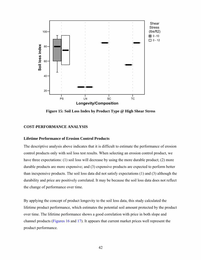
42

PS LN SC TC


20

40

60

80

100

Soil

loss

inde

x


0 -100 - 12

Figure 15: Soil Loss Index by Product Type @ High Shear Stress

COST-PERFORMANCE ANALYSIS

Lifetime Performance of Erosion Control Products

The descriptive analysis above indicates that it is difficult to estimate the performance of erosion

control products only with soil loss test results. When selecting an erosion control product, we

have three expectations: (1) soil loss will decrease by using the more durable product; (2) more

durable products are more expensive; and (3) expensive products are expected to perform better

than inexpensive products. The soil loss data did not satisfy expectations (1) and (3) although the

durability and price are positively correlated. It may be because the soil loss data does not reflect

the change of performance over time.

By applying the concept of product longevity to the soil loss data, this study calculated the

lifetime product performance, which estimates the potential soil amount protected by the product

over time. The lifetime performance shows a good correlation with price in both slope and

channel products (Figures 16 and 17). It appears that current market prices well represent the

product performance.

RESUBMITTAL

43

0 50 100 150 200 250 300

Life-performance (2:1 Clay)

0

10

20

30

40

50Pr

ice

R Sq Linear = 0.659

0 5000 10000 15000 20000 25000

Life-performance (2:1 Sand)

0

10

20

30

40

50

Pric

e

R Sq Linear = 0.729

Figure 16: Correlation between Price and Life-Performance of Slope Protection Products.

0 2000 4000 6000 8000 10000 12000

Life-performance (0 - 2)

0

20

40

60

80

100

120

140

Pric

e

R Sq Linear = 0.504

0 10000 20000 30000

Life-performance (0 - 10)

0

20

40

60

80

100

120

140Pr

ice

R Sq Linear = 0.669

Figure 17: Correlation between Price and Life-Performance of Channel Protection

Products.

Cost-Performance Index of Slope Protection Products

To identify appropriate products for designated conditions such as slope steepness, soil type, and

the expected duration of vegetation establishment, this study calculated the cost-performance

index considering many possible scenarios (i.e., temporary, short-term, mid-term, long-term, and

RESUBMITTAL

44

permanent) by each slope and soil type. The researchers selected appropriate products for each

scenario employing the following rules, which are listed in order of priority.

1. Every scenario should include at least one product.

2. An appropriate product should satisfy a minimum CPI level of 0.5.

3. Price should be reasonable. The acceptable price is set as the larger value of twice the

mean price or minimum price of products listed in the adjacent, higher, longevity

category. Table 15 shows the thresholds of acceptable price for slope protection products.

Table 15: Acceptable Price Threshold for Slope Protection Products.

Longevity Mean Price ($/100 ft2)

Acceptable Price Threshold ($/100 ft2)

Permanent 40 No limit Long 13 34 Mid 8 16

Short 5 10 Temporary 5 10

The overall results indicate that temporary products are better suited for temporary projects;

likewise, long-term products are more useful for long-term projects.

Cost-Performance Index of Channel Protection Products

After calculating the CPI of channel protection products for every scenario, the selection of

appropriate products is made according to the rules explained above. Table 16 shows the

threshold of acceptable price for channel products.

Table 16: Acceptable Price Threshold for Channel Protection Products

Longevity Mean Price ($/100 ft2)

Acceptable Price Threshold ($/100 ft2)

Permanent 37 No limit Long 26 52 Mid 22 44

Short 6 18 Temporary 6 9

Affordable long-term channel products can be widely used for temporary to mid-term projects.

Permanent products are frequently recommended for longer term projects.

RESUBMITTAL

45

USER’S GUIDE TO SUGGESTED APL In order to use the suggested APL, site- or project-specific information is needed, including: (1) Protection type – slope or channel (2) Soil type – clay or sand (3) Stress – steepness of slope or shear stress of flow in channel (4) Anticipated project duration The selection process of products follows the decision tree below. Each box lists the needed data for making a decision to move forward to the next step.

An example below is used to illustrate each slope and channel product selection process. A 12-month highway expansion project includes a 3:1 slope that is adjacent to a drainage swale at the bottom of the slope. The swale has a depth of 12 inches and 5% longitudinal slope. The soil type is clay. To protect the slope, products approved for 3:1 clay that will last 12-month should be selected. Hence, select any product from the “Short-term (12 months)” column of the “Clay 3:1” table. To protect the channel, estimating shear stress is needed. The shear stress (τ) on an open channel can be calculated using τ = γds, where γ is fluid specific gravity, d is the depth of the flow and s is the longitudinal slope of the channel. The shear stress of the drainage swale is calculated: τ = γds = 62.4 lb/ft3 × 1ft × 0.05 = 3.1 lb/ft2. Therefore, select any product from the “Short-term (12 months)” column of the “Shear Stress: 0 ~ 4” table.

Protection Type

Soil Type Steepness

Project Duration

Shear Stress Project Duration

Slope Channel

Product Selection

Product Selection

RESUBMITTAL

46

RESUBMITTAL

47

REFERENCES CALTRANS. 2000. District 7 Erosion Control Pilot Study: California Department of

Transportation.

Doring, T., M. Brandt, J. Heb, M. Finckh, and H. Saucke. 2005. Effects of straw mulch on soil nitrate dynamics, weeds, yield and soil erosion in organically grown potatoes. Field Crops Research 94:238-249.

Edwards, L., J. Burney, G. Richter, and A. MacRae. 2000. Evaluation of compost and straw mulching on soil loss characteristics in erosion plots of potatoes in Prince Edward Island, California. Agriculture, Ecosystem and Environment 81:217-222.

Godfrey, S., and J. Long. 1994. Temporary erosion control measures design guidelines for TxDOT: Texas Department of Transportation.

IWR. 2005. RUSLE: On-line soil erosion assessment tool. Institute of Water Research, Michigan State University 2002 [cited 2005]. Available from http://www.iwr.msu.edu/rusle/.

Li, M., Landphair, H.C., McFalls, J. 2003. Comparison of field and laboratory experiment test results for erosion control products. American Society of Agricultural Engineers Paper No. 032352. Las Vegas, NV: ASAE.

Northcutt, P., and McFalls, J. 1997. Field Performance Testing of Selected Erosion Control Products Final Performance Analysis Through the 1996 Evaluation Cycle: Texas Department of Transportation.

NCDAS. 2005. Plant nutrients. North Carolina Dept. of Agriculture & Consumer Services 1994 [cited 2005]. Available from http://www.agr.state.nc.us/cyber/kidswrld/plant/nutrient.htm.

Persyn, R., T. Glanville, T. Richard, J. Laflen, and P. Dixon. 2005. Environmental effects of applying composted organics to new highway embankments: Part III. Rill erosion. American Society of Agricultural Engineers 48 (5):1765-1772.

Puppala, A., Intharasombat, N., and Qasim, S., 2004. The effects of using compost as a preventive measure to mitigate shoulder cracking: Laboratory and field studies: University of Texas at Arlington.

Roose, E. 1996. Land husbandry - Components and strategy: Food and Agriculture Organization of the United Nations.

Smith, D.D. and W.H. Wischmeier. 1957. Factors affecting sheet and rill erosion. Trans. Am. Geophys. Union 38:889-896.

Storey, B., McFalls, J., and Godfrey, S.. 1996. The use of compost and shredded brush on rights-of-way for erosion control: Texas Transportation Institute.

TxDOT, 2005. Final Performance Analysis Through 2004 Evaluation Cycles--Slope Protection

RESUBMITTAL

http://www.iwr.msu.edu/rusle/

http://www.agr.state.nc.us/cyber/kidswrld/plant/nutrient.htm

48

Products, Flexible Channel Liner Products & Hydraulic Mulches. Vegetation Management Section of Maintenance Division, Texas Department of Transportation.

TxDOT, 2000. Final Performance Analysis Through 1999 Evaluation Cycles--Slope Protection Products, Flexible Channel Liner Products & Hydraulic Mulches. Texas Department of Transportation.

USCC. 2001. Field guide to compost use: US Composting Council.

———. 2005. Evaluating compost quality. US Composting Council 2005 [cited 2005]. Available from http://www.compostingcouncil.org/section.cfm?id=39.

Wischmeier, W., and D. Smith. 1978. Predicting rainfall erosion losses - A guide to conservation planning. In US Dept Ag. (USDA) Handbook No. 537.

RESUBMITTAL

http://www.compostingcouncil.org/section.cfm?id=39

49

APPENDIX A Suggested Approved Products List after the Cost-Performance Analysis,

Slope Protection Products

RESUBMITTAL

RESUBMITTAL

51

Suggested Approved Products List after Cost-Performance Analysis, Slope Protection Products

RE

SU

BM

ITT

AL

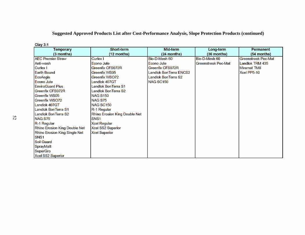
52

Suggested Approved Products List after Cost-Performance Analysis, Slope Protection Products (continued)

RE

SU

BM

ITT

AL

53


RE

SU

BM

ITT

AL

54


RE

SU

BM

ITT

AL

55

APPENDIX B Suggested Approved Products List After the Cost-Performance Analysis,

Channel Protection Products

RESUBMITTAL

RESUBMITTAL

57

Suggested Approved Products List after Cost-Performance Analysis, Channel Protection Products

RE

SU

BM

ITT

AL

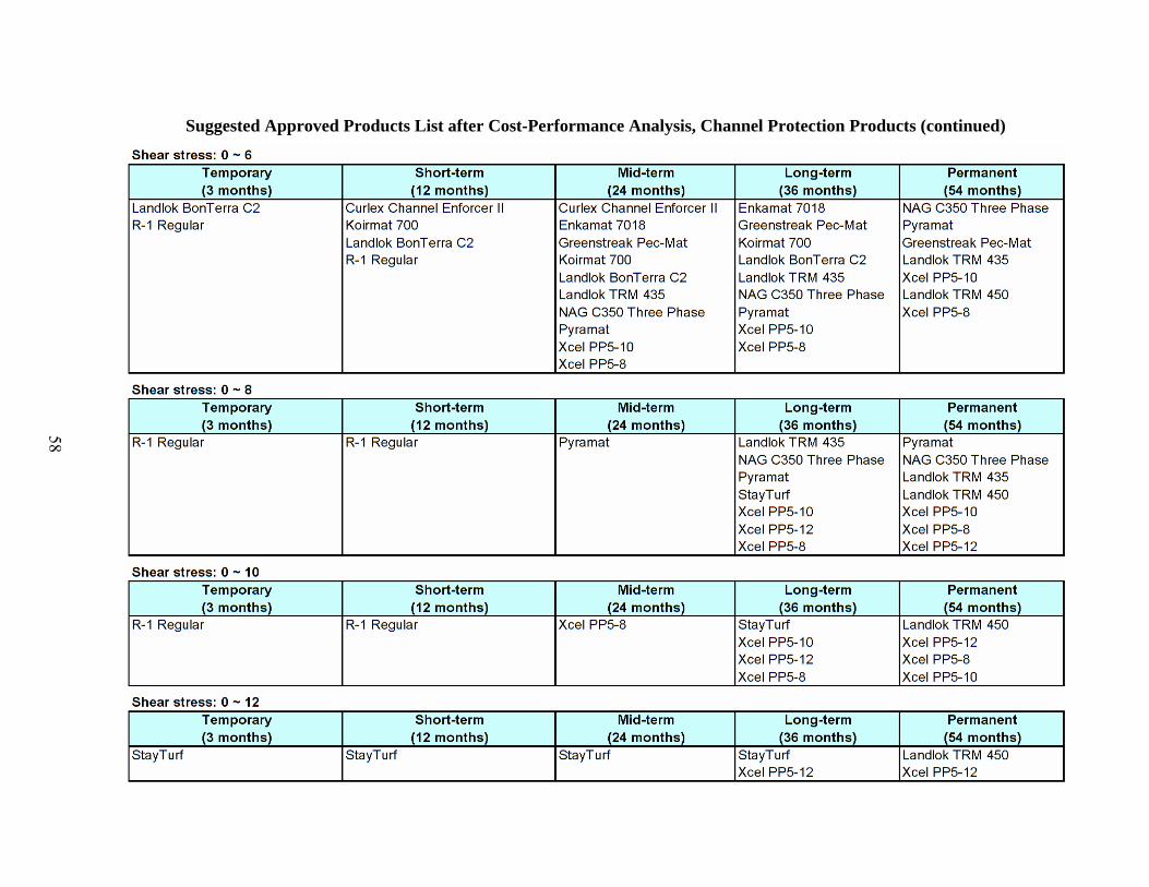
58

Suggested Approved Products List after Cost-Performance Analysis, Channel Protection Products (continued)

RE

SU

BM

ITT

AL

59

APPENDIX C TxDOT APPROVED PRODUCT LIST

SEPTEMBER 2006

RESUBMITTAL

RESUBMITTAL

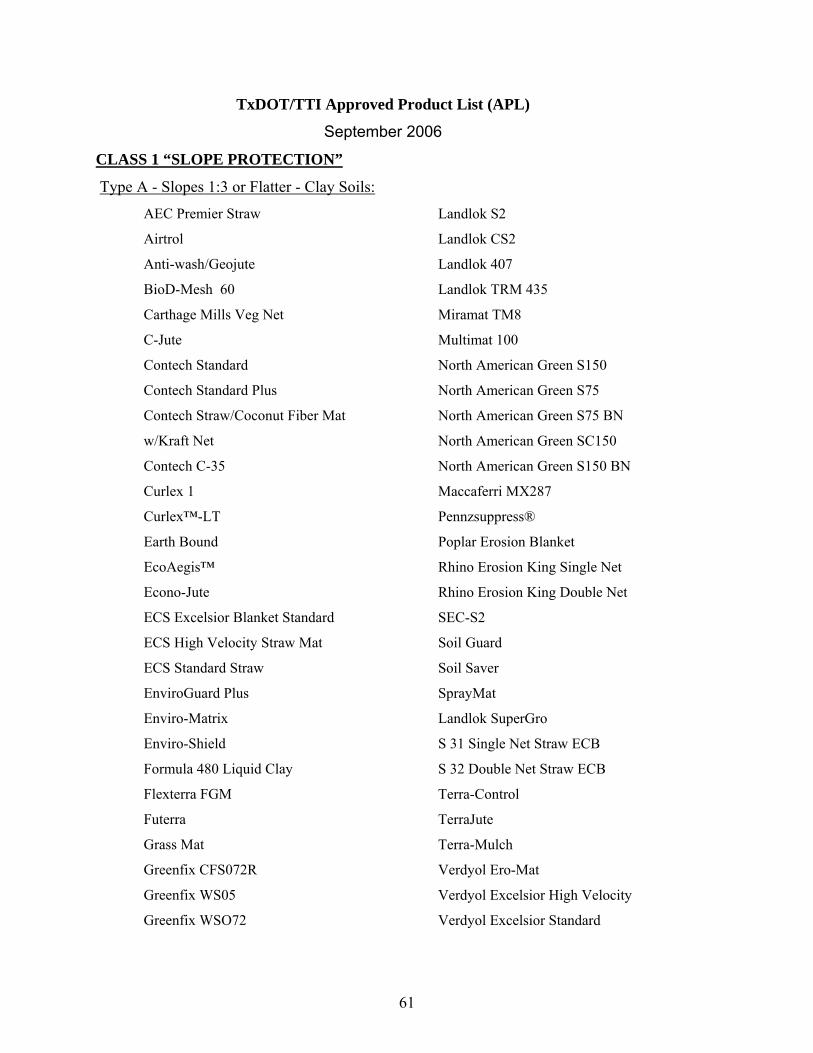
61

TxDOT/TTI Approved Product List (APL)

September 2006

CLASS 1 “SLOPE PROTECTION”

Type A - Slopes 1:3 or Flatter - Clay Soils:

AEC Premier Straw

Airtrol

Anti-wash/Geojute

BioD-Mesh 60

Carthage Mills Veg Net

C-Jute

Contech Standard

Contech Standard Plus

Contech Straw/Coconut Fiber Mat

w/Kraft Net

Contech C-35

Curlex 1

Curlex™-LT

Earth Bound

EcoAegis™

Econo-Jute

ECS Excelsior Blanket Standard

ECS High Velocity Straw Mat

ECS Standard Straw

EnviroGuard Plus

Enviro-Matrix

Enviro-Shield

Formula 480 Liquid Clay

Flexterra FGM

Futerra

Grass Mat

Greenfix CFS072R

Greenfix WS05

Greenfix WSO72

Landlok S2

Landlok CS2

Landlok 407

Landlok TRM 435

Miramat TM8

Multimat 100

North American Green S150


North American Green S75 BN

North American Green SC150


Maccaferri MX287

Pennzsuppress®

Poplar Erosion Blanket

Rhino Erosion King Single Net

Rhino Erosion King Double Net

SEC-S2

Soil Guard

Soil Saver

SprayMat

Landlok SuperGro

S 31 Single Net Straw ECB

S 32 Double Net Straw ECB

Terra-Control

TerraJute

Terra-Mulch

Verdyol Ero-Mat

Verdyol Excelsior High Velocity

Verdyol Excelsior Standard

RESUBMITTAL

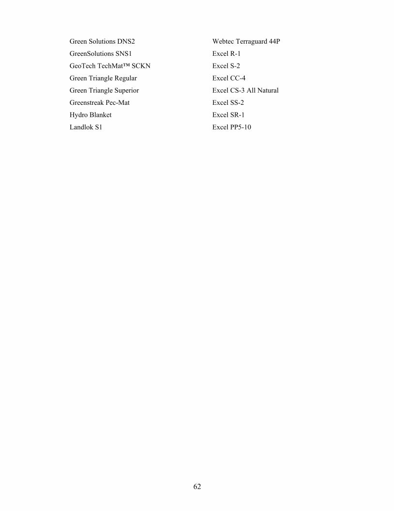
62

Green Solutions DNS2

GreenSolutions SNS1

GeoTech TechMat™ SCKN

Green Triangle Regular

Green Triangle Superior

Greenstreak Pec-Mat

Hydro Blanket

Landlok S1

Webtec Terraguard 44P

Excel R-1

Excel S-2

Excel CC-4

Excel CS-3 All Natural

Excel SS-2

Excel SR-1

Excel PP5-10

RESUBMITTAL

63

CLASS 1 “SLOPE PROTECTION” (continued)

Type B - 1:3 or Flatter - Sandy Soils:

AEC Premier

C-Jute


Contech Standard



w/Kraft Net

Contech C-35

Curlex 1

Curlex LT

Earth Bound

EarthGuard Fiber Matrix

ECS Standard Straw

ECS Excelsior Blanket Standard


EnviroGuard Plus

Flexterra FGM

Futerra

Greenfix CFS072R

Greenfix WS05

Greenfix WSO72

GreenSolutions SNS1

Geojute Plus 1


Green Triangle Regular


Landlok S1

Landlok S2

Landlok CS2

Landlok 407

Landlok TRM 435

Maccaferri MX287

Miramat 1000

Miramat TM8

Multimat 100





North American Green® S150 BN



SEC-S2

Soil Guard

S 31 Single Net Straw ECB


Terra-Control

TerraJute

Verdyol Ero-Mat

Verdyol Excelsior Standard


Excel R-1

Excel S-2

Excel CC-4


Excel CS-3

Excel SS-2

Excel 5-8

Excel PP5-10

Excel PP5-12

RESUBMITTAL

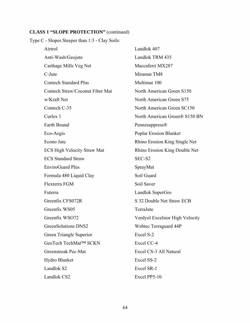
64


Type C - Slopes Steeper than 1:3 - Clay Soils:

Airtrol

Anti-Wash/Geojute


C-Jute



w/Kraft Net

Contech C-35

Curlex 1

Earth Bound

Eco-Aegis

Econo Jute


ECS Standard Straw

EnviroGuard Plus

Formula 480 Liquid Clay

Flexterra FGM

Futerra

Greenfix CFS072R

Greenfix WS05

Greenfix WSO72

GreenSolutions DNS2



Greenstreak Pec-Mat

Hydro Blanket

Landlok S2

Landlok CS2

Landlok 407

Landlok TRM 435

Maccaferri MX287

Miramat TM8

Multimat 100




North American Green® S150 BN

Pennzsuppress®




SEC-S2

SprayMat

Soil Guard

Soil Saver

Landlok SuperGro


TerraJute

Verdyol Excelsior High Velocity


Excel S-2

Excel CC-4


Excel SS-2

Excel SR-1

Excel PP5-10

RESUBMITTAL

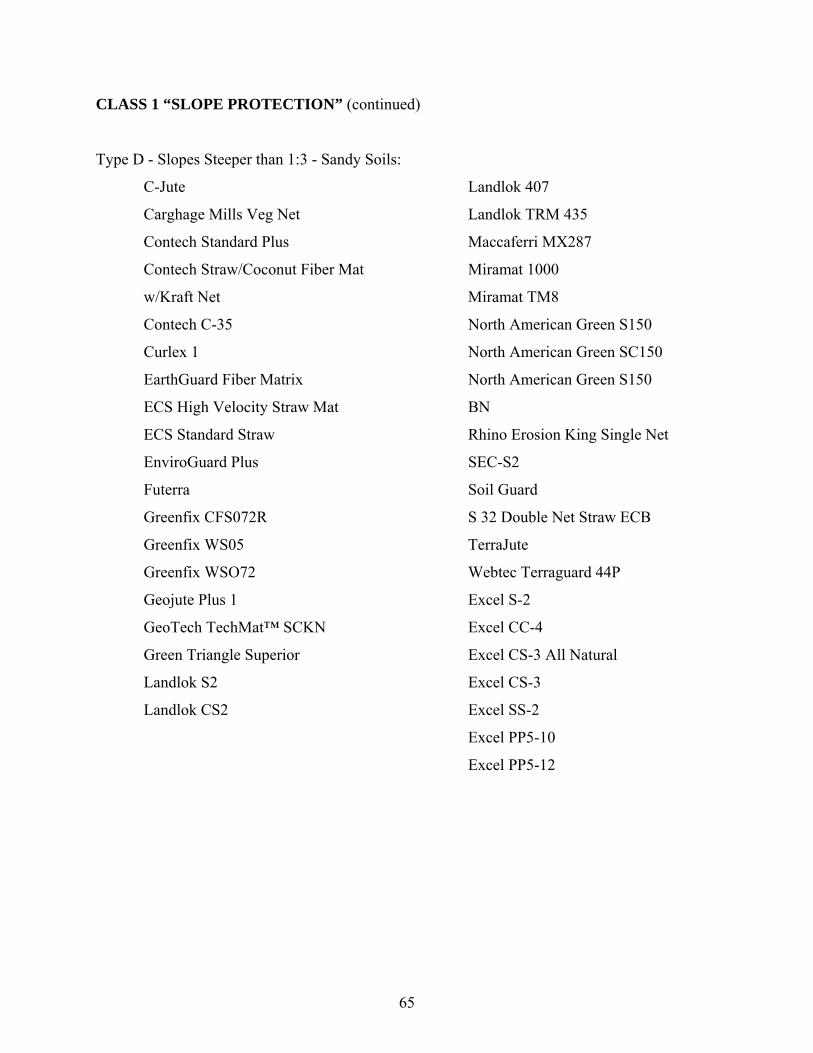
65


Type D - Slopes Steeper than 1:3 - Sandy Soils:

C-Jute

Carghage Mills Veg Net



w/Kraft Net

Contech C-35

Curlex 1

EarthGuard Fiber Matrix


ECS Standard Straw

EnviroGuard Plus

Futerra

Greenfix CFS072R

Greenfix WS05

Greenfix WSO72

Geojute Plus 1



Landlok S2

Landlok CS2

Landlok 407

Landlok TRM 435

Maccaferri MX287

Miramat 1000

Miramat TM8




BN


SEC-S2

Soil Guard


TerraJute


Excel S-2

Excel CC-4


Excel CS-3

Excel SS-2

Excel PP5-10

Excel PP5-12

RESUBMITTAL

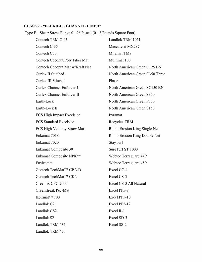
66

CLASS 2 - “FLEXIBLE CHANNEL LINER”

Type E - Shear Stress Range 0 - 96 Pascal (0 - 2 Pounds Square Foot):

Contech TRM C-45

Contech C-35

Contech C50

Contech Coconut/Poly Fiber Mat

Contech Coconut Mat w/Kraft Net

Curlex II Stitched

Curlex III Stitched

Curlex Channel Enforcer 1

Curlex Channel Enforcer II

Earth-Lock

Earth-Lock II

ECS High Impact Excelsior

ECS Standard Excelsior


Enkamat 7018

Enkamat 7020

Enkamat Composite 30

Enkamat Composite NPK**

Enviromat

Geotech TechMat™ CP 3-D

Geotech TechMat™ CKN

Greenfix CFG 2000

Greenstreak Pec-Mat

Koirmat™ 700

Landlok C2

Landlok CS2

Landlok S2

Landlok TRM 435

Landlok TRM 450

Landlok TRM 1051

Maccaferri MX287

Miramat TM8

Multimat 100

North American Green C125 BN

North American Green C350 Three

Phase

North American Green SC150 BN


North American Green P350


Pyramat

Recyclex TRM



StayTurf

SureTurf ST 1000



Excel CC-4

Excel CS-3


Excel PP5-8

Excel PP5-10

Excel PP5-12

Excel R-1

Excel SD-3

Excel SS-2

RESUBMITTAL

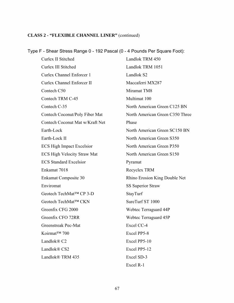
67

CLASS 2 - “FLEXIBLE CHANNEL LINER” (continued)

Type F - Shear Stress Range 0 - 192 Pascal (0 - 4 Pounds Per Square Foot):

Curlex II Stitched

Curlex III Stitched

Curlex Channel Enforcer 1


Contech C50

Contech TRM C-45

Contech C-35


Contech Coconut Mat w/Kraft Net

Earth-Lock

Earth-Lock II

ECS High Impact Excelsior


ECS Standard Excelsior

Enkamat 7018


Enviromat


Geotech TechMat™ CKN

Greenfix CFG 2000

Greenfix CFO 72RR

Greenstreak Pec-Mat

Koirmat™ 700

Landlok® C2

Landlok® CS2

Landlok® TRM 435

Landlok TRM 450

Landlok TRM 1051

Landlok S2

Maccaferri MX287

Miramat TM8

Multimat 100

North American Green C125 BN


Phase

North American Green SC150 BN




Pyramat

Recyclex TRM


SS Superior Straw

StayTurf

SureTurf ST 1000



Excel CC-4

Excel PP5-8

Excel PP5-10

Excel PP5-12

Excel SD-3

Excel R-1

RESUBMITTAL

68


Type G - Shear Stress Range 0 - 287 Pascal (0 - 6 Pounds Square Foot):

Contech TRM C-45

Contech C-35

Contech C50



Earth-Lock

Earth-Lock II

Enkamat 7018



Greenfix CFG 2000

Greenstreak Pec-Mat

Koirmat™ 700

Landlok BonTerra® CP2

Landlok TRM 1051

Landlok TRM 1060

Landlok TRM 435

Landlok TRM 450

Multimat 100


Phase


North American Green® P350

Pyramat

Recyclex TRM

StayTurf

SureTurf ST 1000



Excel PP5-8

Excel PP5-10

Excel PP5-12


Type H - Shear Stress Range 0 - 383 Pascal (0 - 8 Pounds Square Foot):

Contech TRM C-45

Contech C-35

Contech C50



Landlok TRM 435

Landlok TRM 450

Landlok TRM 1051

Multimat 100


Phase



Pyramat

Recyclex TRM

StayTurf

SureTurf ST 1000



Excel PP5-8

Excel PP5-10

Excel PP5-12

RESUBMITTAL

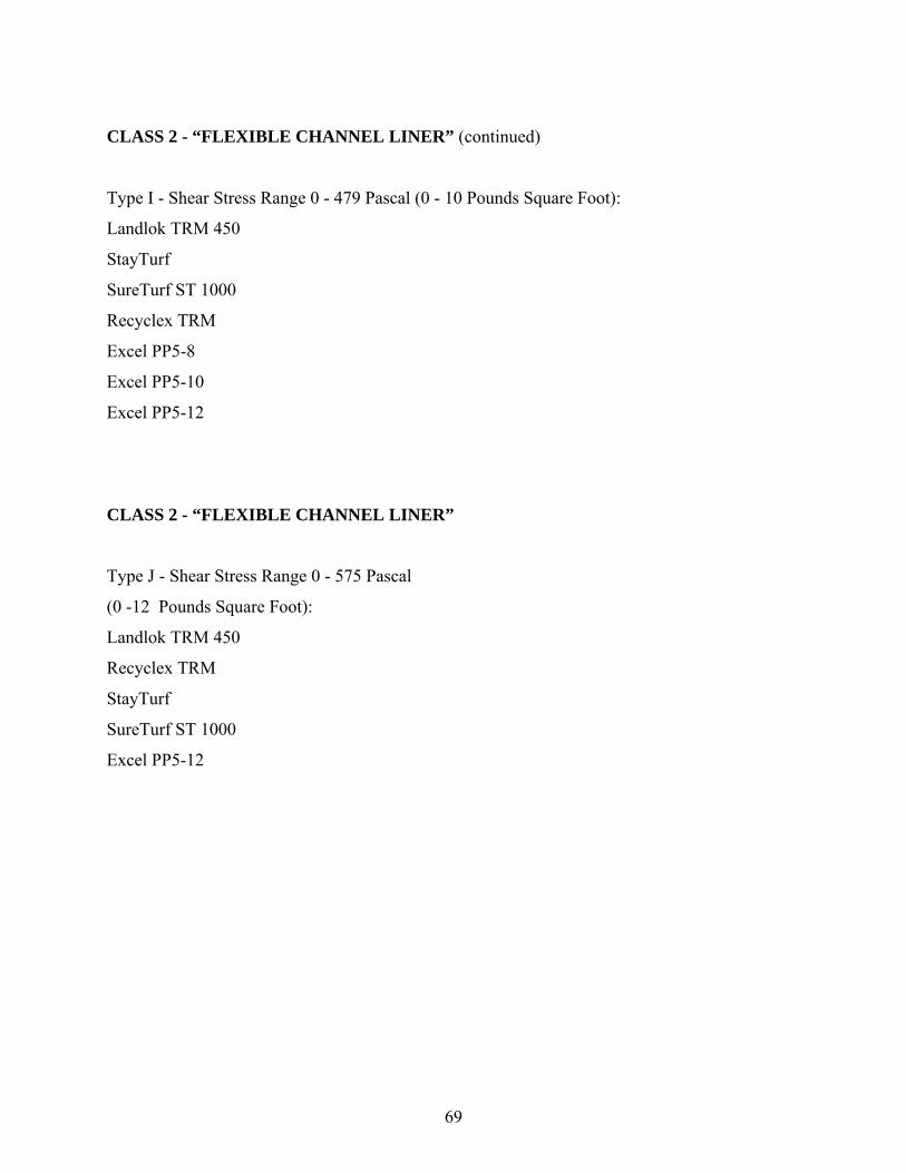
69


Type I - Shear Stress Range 0 - 479 Pascal (0 - 10 Pounds Square Foot):

Landlok TRM 450

StayTurf

SureTurf ST 1000

Recyclex TRM

Excel PP5-8

Excel PP5-10

Excel PP5-12

CLASS 2 - “FLEXIBLE CHANNEL LINER”

Type J - Shear Stress Range 0 - 575 Pascal

(0 -12 Pounds Square Foot):

Landlok TRM 450

Recyclex TRM

StayTurf

SureTurf ST 1000

Excel PP5-12

RESUBMITTAL

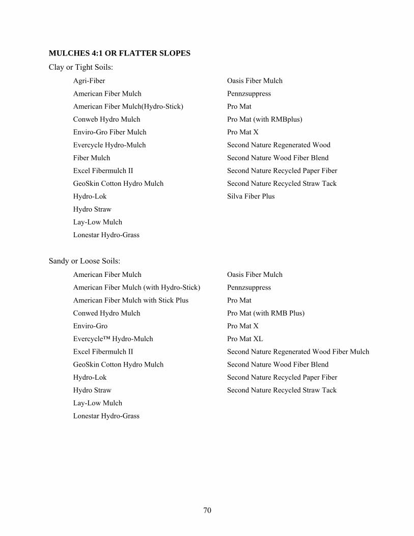
70

MULCHES 4:1 OR FLATTER SLOPES

Clay or Tight Soils:

Agri-Fiber

American Fiber Mulch

American Fiber Mulch(Hydro-Stick)

Conweb Hydro Mulch

Enviro-Gro Fiber Mulch

Evercycle Hydro-Mulch

Fiber Mulch

Excel Fibermulch II

GeoSkin Cotton Hydro Mulch

Hydro-Lok

Hydro Straw

Lay-Low Mulch

Lonestar Hydro-Grass

Oasis Fiber Mulch

Pennzsuppress

Pro Mat

Pro Mat (with RMBplus)

Pro Mat X

Second Nature Regenerated Wood

Second Nature Wood Fiber Blend

Second Nature Recycled Paper Fiber

Second Nature Recycled Straw Tack

Silva Fiber Plus

Sandy or Loose Soils:

American Fiber Mulch

American Fiber Mulch (with Hydro-Stick)

American Fiber Mulch with Stick Plus

Conwed Hydro Mulch

Enviro-Gro

Evercycle™ Hydro-Mulch

Excel Fibermulch II

GeoSkin Cotton Hydro Mulch

Hydro-Lok

Hydro Straw

Lay-Low Mulch

Lonestar Hydro-Grass

Oasis Fiber Mulch

Pennzsuppress

Pro Mat

Pro Mat (with RMB Plus)

Pro Mat X

Pro Mat XL

Second Nature Regenerated Wood Fiber Mulch

Second Nature Wood Fiber Blend

Second Nature Recycled Paper Fiber

Second Nature Recycled Straw Tack

RESUBMITTAL

Cost Performance Index of Temporary Erosion Control Products

Documents