Chapter Twenty-One Cost Curves 成成成成

Welcome message from author
This document is posted to help you gain knowledge. Please leave a comment to let me know what you think about it! Share it to your friends and learn new things together.
Transcript
Chapter Twenty-One
Cost Curves成本曲线

7 Types of Cost Curves
A total cost curve (总成本曲线) is the graph of a firm’s total cost function.
An average total cost curve (平均成本曲线) is the graph of a firm’s average total cost function.
A variable cost curve (可变成本曲线) is the graph of a firm’s variable cost function.
An average variable cost curve (平均可变成本曲线) is the graph of a firm’s average variable cost function.

7 Types of Cost Curves
An fixed cost curve (固定成本曲线) is the graph of a firm’s fixed cost function.
An average fixed cost curve (平均固定成本曲线) is the graph of a firm’s average fixed cost function.
A marginal cost curve (边际成本曲线) is the graph of a firm’s marginal cost function.

7 Types of Cost Curves
How are these cost curves related to each other?
How are a firm’s long-run and short-run cost curves related?

Fixed, Variable & Total Cost Functions
F is the firm’s fixed cost, It’s the total cost to a firm’s short-
run fixed inputs (固定投入) . does not vary with the firm’s
output level. cv(y) is the firm’s variable cost
function. cv(y) is the total cost to a firm of
its variable inputs (可变投入) when producing y output units.

Fixed, Variable & Total Cost Functions
c(y) is the total cost of all inputs, fixed and variable, when producing y output units. c(y) is the firm’s total cost function;
c y F c yv( ) ( ).

y
$
F

y
$
cv(y)

y
$
F
cv(y)

y
$
F
cv(y)
c(y)
F
c y F c yv( ) ( )
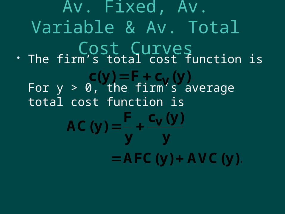
Av. Fixed, Av. Variable & Av. Total Cost Curves
The firm’s total cost function is
For y > 0, the firm’s average total cost function is
c y F c yv( ) ( ).
AC yFy
c yy
AFC y AVC y
v( )( )
( ) ( ).

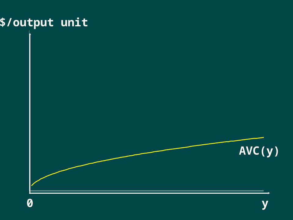
Av. Fixed, Av. Variable & Av. Total Cost Curves
What does an average fixed cost curve look like?
AFC(y) graph looks like ...
AFC yFy
( )

$/output unit
AFC(y)
y0
AFC(y) 0 as y
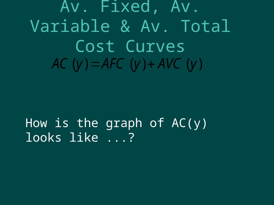
Av. Fixed, Av. Variable & Av. Total Cost Curves
).()()( yAVCyAFCyAC
How is the graph of AC(y) looks like ...?
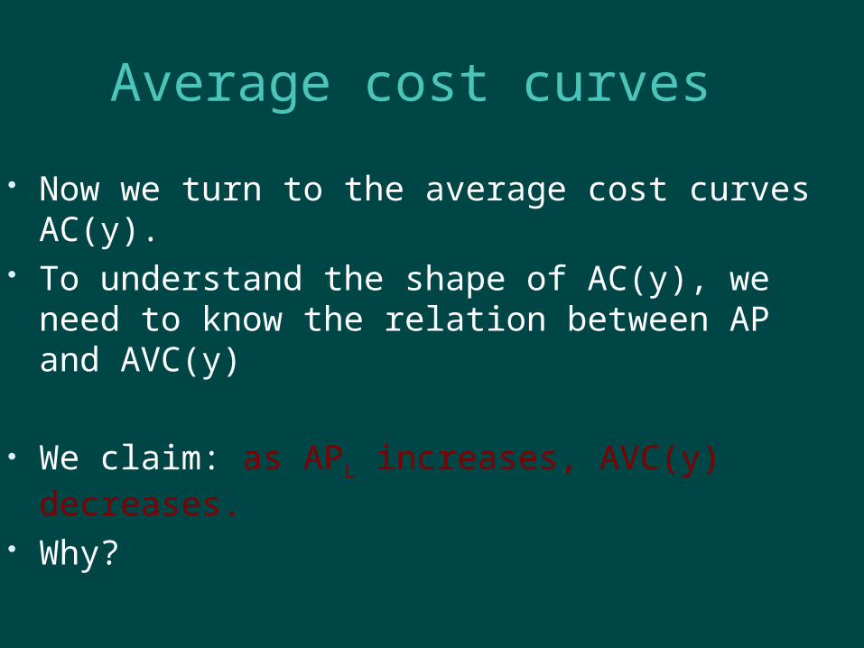
Average cost curves
Now we turn to the average cost curves AC(y).
To understand the shape of AC(y), we need to know the relation between AP and AVC(y)
We claim: as APL increases, AVC(y) decreases.
Why?
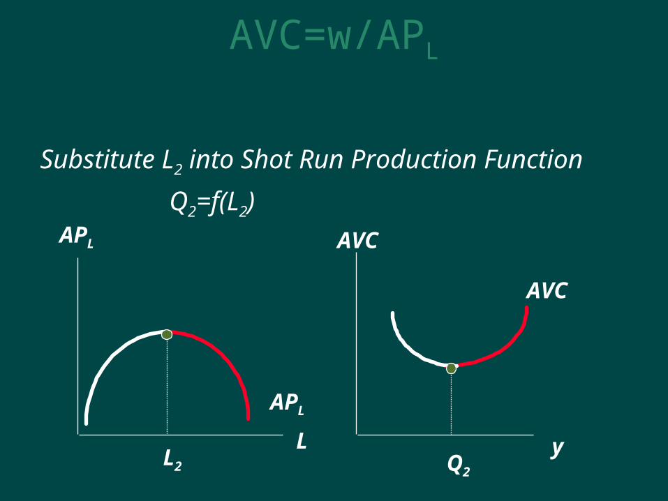
AVC=w/APL
APL
Substitute L2 into Shot Run Production Function
Q2=f(L2)
LL2
AVC
y
AVC
Q2
APL
$/output unit
AVC(y)
y0

$/output unit
AFC(y)
AVC(y)
y0
Av. Fixed, Av. Variable & Av. Total Cost Curves
And ATC(y) = AFC(y) + AVC(y)

$/output unit
AFC(y)
AVC(y)
ATC(y)
y0
ATC(y) = AFC(y) + AVC(y)

$/output unit
AFC(y)
AVC(y)
ATC(y)
y0
AFC(y) = ATC(y) - AVC(y)
AFC

$/output unit
AFC(y)
AVC(y)
ATC(y)
y0
Since AFC(y) 0 as y ,ATC(y) AVC(y) as y
AFC

$/output unit
AFC(y)
AVC(y)
ATC(y)
y0
Since AFC(y) 0 as y ,ATC(y) AVC(y) as y
And since short-run AVC(y) musteventually increase, ATC(y) must eventually increase in a short-run.

Marginal Cost Function
Marginal cost is the rate-of-change of variable production cost as the output level changes. That is,
MC yc yyv( )( ).

Marginal Cost Function
The firm’s total cost function is
and the fixed cost F does not change with the output level y, so
MC is the slope of both the variable cost and the total cost functions.
c y F c yv( ) ( )
MC yc yy
c yy
v( )( ) ( )
.

Av. Fixed, Av. Variable & Av. Total Cost Curves
How is the graph of MC(y) looks like ...?
Recall the law of deminishing marginal returns( 边际收益递减规律 ) ?

MC=w/MPL
An Example of Marginal Production of Labor input
MPL
LL1
MC
y
Look at where Diminishing Returns begin
MPL

MC=w/MPL
An Example of Marginal Production of Labor input
Look at where Diminishing Returns begin
LL1y
MC
Q1
MPL
MPLMC

Av. Fixed, Av. Variable & Av. Total Cost Curves
the Law of Diminishing (Marginal) Returns must cause the firm’s marginal cost of production to increase eventually.
That is, at the beginning as MPL
increases, MC decreases; And later as MPL decreases, MC
increases.

Relation between MC(y) and cv(y)
Since MC(y) is the derivative of cv(y), cv(y) must be the integral of MC(y). That is,
MC yc yyv( )( )
c y MC z dzv
y( ) ( ) .
0

MC(y)
y0
c y MC z dzv
y( ) ( )
0
y
Area is the variablecost of making y’ units
$/output unit
Relation between MC(y) and cv(y)

Relation between MC(y) and AVC(y)
How is marginal cost related to average variable cost?

Relation between MC(y) and AVC(y)
Since AVC yc yyv( )( ),
AVC yy
y MC y c y
yv( ) ( ) ( )
. 1
2

Relation between MC(y) and AVC(y)
Since AVC yc yyv( )( ),
AVC yy
y MC y c y
yv( ) ( ) ( )
. 1
2
Therefore,
AVC yy( )
0 y MC y c yv
( ) ( ).as

Relation between MC(y) and AVC(y)
Since AVC yc yyv( )( ),
AVC yy
y MC y c y
yv( ) ( ) ( )
. 1
2
Therefore,
AVC yy( )
0 y MC y c yv
( ) ( ).as
MC yc yy
AVC yv( )( )
( ).
as
AVC yy( )
0

$/output unit
y
AVC(y)
MC(y)

$/output unit
y
AVC(y)
MC(y)
MC y AVC yAVC yy
( ) ( )( )
0

$/output unit
y
AVC(y)
MC(y)
MC y AVC yAVC yy
( ) ( )( )
0

$/output unit
y
AVC(y)
MC(y)
MC y AVC yAVC yy
( ) ( )( )
0

$/output unit
y
AVC(y)
MC(y)
MC y AVC yAVC yy
( ) ( )( )
0
The short-run MC curve intersectsthe short-run AVC curve frombelow at the AVC curve’s minimum.

Relation between MC(y) and ATC(y)
Similarly, since ATC yc yy
( )( ),
ATC yy
y MC y c y
y
( ) ( ) ( ).
12

Relation between MC(y) and ATC(y)
Similarly, since ATC yc yy
( )( ),
ATC yy
y MC y c y
y
( ) ( ) ( ).
12
Therefore,
ATC yy( )
0 y MC y c y
( ) ( ).as

Relation between MC(y) and ATC(y)
Similarly, since ATC yc yy
( )( ),
ATC yy
y MC y c y
y
( ) ( ) ( ).
12
Therefore,
ATC yy( )
0 y MC y c y
( ) ( ).as
MC yc yy
ATC y( )( )
( ).
as
ATC yy( )
0
$/output unit
y
MC(y)
ATC(y)
MC y ATC y( ) ( )
as
ATC yy( )
0

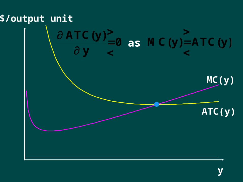
Relation between MC(y) and ATC(y)
The short-run MC curve intersects the short-run AVC curve from below at the AVC curve’s minimum.
And, similarly, the short-run MC curve intersects the short-run ATC curve from below at the ATC curve’s minimum.

$/output unit
y
AVC(y)
MC(y)
ATC(y)
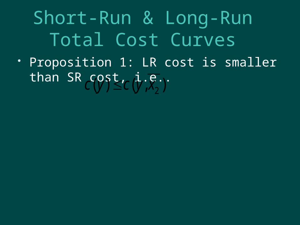
Short-Run & Long-Run Total Cost Curves
Proposition 1: LR cost is smaller than SR cost, i.e..
2( ) ( , )c y c y x

LR cost is smaller than SR cost
Reason: To increase output, in the long run, a firm can adjust all factors; in the short-run, the firm can only some factors.
Long-run production is more flexible It has been shown with the help of LR and
SR expansion paths (in chapter 20). Now we show it with the help of total cost
curves.

Short-Run & Long-Run Total Costs
x1
x2
y
y
y
x1 x1 x1
x2x2x2
Short-runoutputexpansionpath
Long-run costs are:c y w x w xc y w x w xc y w x w x
( )( )( )
1 1 2 2
1 1 2 2
1 1 2 2

Short-Run & Long-Run Total Costs
x1
x2
y
y
y
x1 x1 x1
x2x2x2
Short-runoutputexpansionpath
Long-run costs are:c y w x w xc y w x w xc y w x w x
( )( )( )
1 1 2 2
1 1 2 2
1 1 2 2Short-run costs are:
c y c ys ( ) ( )

Short-Run & Long-Run Total Costs
x1
x2
y
y
y
x1 x1 x1
x2x2x2
Short-runoutputexpansionpath
Long-run costs are:c y w x w xc y w x w xc y w x w x
( )( )( )
1 1 2 2
1 1 2 2
1 1 2 2
Short-run costs are:c y c yc y c ys
s
( ) ( )( ) ( )

Short-Run & Long-Run Total Costs
x1
x2
y
y
y
x1 x1 x1
x2x2x2
Short-runoutputexpansionpath
Long-run costs are:c y w x w xc y w x w xc y w x w x
( )( )( )
1 1 2 2
1 1 2 2
1 1 2 2
Short-run costs are:
)()(
)()(
)()(
ycyc
ycyc
ycyc
s
s
s
•one point in common )()( ycycs

Short-Run & Long-Run Total Costs
This says that the long-run total cost curve always has one point in common with any particular short-run total cost curve.
Short-run total cost exceeds long-run total cost except for the output level where the short-run input level restriction is the long-run input level choice.

Short-Run & Long-Run Total Costs
y
$
c(y)
yyy
cs(y)
Fw x
2 2
A short-run total cost curve always hasone point in common with the long-runtotal cost curve, and is elsewhere higherthan the long-run total cost curve.

Short-Run & Long-Run Total Cost Curves
A firm has a different short-run total cost curve for each possible short-run circumstance.
Suppose the firm can be in one of just three short-runs; x2 = x2 or x2 = x2 x2 < x2 < x2.or x2 = x2.

y0
F = w2x2
F
cs(y;x2)
$

y
F0
F = w2x2
F
F = w2x2
cs(y;x2)
cs(y;x2)
$

y
F0
F = w2x2F = w2x2
A larger amount of the fixedinput increases the firm’sfixed cost.
cs(y;x2)
cs(y;x2)
$
F

y
F0
F = w2x2F =
w2x2A larger amount of the fixedinput increases the firm’sfixed cost.
Why does a larger amount of the fixed input reduce the slope of the firm’s total cost curve?
cs(y;x2)
cs(y;x2)
$
F

MP1 is the marginal physical productivityof the variable input 1, so one extra unit ofinput 1 gives MP1 extra output units.Therefore, the extra amount of input 1needed for 1 extra output unit is
Short-Run & Long-Run Total Cost Curves
units of input 1.1MP/1

MP1 is the marginal physical productivityof the variable input 1, so one extra unit ofinput 1 gives MP1 extra output units.Therefore, the extra amount of input 1needed for 1 extra output unit is
Short-Run & Long-Run Total Cost Curves
MCwMP
1
1.
units of input 1.Each unit of input 1 costs w1, so the firm’sextra cost from producing one extra unitof output is
1MP/1

Short-Run & Long-Run Total Cost Curves
MCwMP
1
1is the slope of the firm’s total cost curve.

Short-Run & Long-Run Total Cost Curves
MCwMP
1
1is the slope of the firm’s total cost curve.
If input 2 is a complement to input 1 thenMP1 is higher for higher x2.Hence, MC is lower for higher x2.
That is, a short-run total cost curve startshigher and has a lower slope if x2 is larger.

y
F0
F = w2x2F =
w2x2
F
F = w2x2
cs(y;x2)
cs(y;x2)
cs(y;x2)
$
F

Short-Run & Long-Run Total Cost Curves
The firm has three short-run total cost curves.
In the long-run the firm is free to choose amongst these three since it is free to select x2 equal to any of x2, x2, or x2.
How does the firm make this choice?

y
F0
F
y y
For 0 y y, choose x2 = x2.
cs(y;x2)
cs(y;x2)
cs(y;x2)
$
F

y
F0
F
y y
For 0 y y, choose x2 = x2.For y y y, choose x2 = x2.
cs(y;x2)
cs(y;x2)
cs(y;x2)
$
F

y
F0
F
cs(y;x2)
y y
For 0 y y, choose x2 = x2.For y y y, choose x2 = x2.For y y, choose x2 = x2.
cs(y;x2)
cs(y;x2)
$
F

y
F0
cs(y;x2)
cs(y;x2)
F
cs(y;x2)
y y
For 0 y y, choose x2 = x2.For y y y, choose x2 = x2.For y y, choose x2 = x2.
c(y), thefirm’s long-run totalcost curve.
$
F

Short-Run & Long-Run Total Cost Curves
The firm’s long-run total cost curve consists of the lowest parts of the short-run total cost curves.
The long-run total cost curve is the lower envelope ( 下包络线 ) of the short-run total cost curves.

Short-Run & Long-Run Total Cost Curves
If input 2 is available in continuous amounts then there is an infinity (无数多) of short-run total cost curves but the long-run total cost curve is still the lower envelope of all of the short-run total cost curves.

$
y
F0
F
cs(y;x2)
cs(y;x2)
cs(y;x2)
c(y)
F

Short-Run & Long-Run Average Total Cost Curves For any output level y, the long-run
total cost curve always gives the lowest possible total production cost.
Therefore, the long-run av. total cost curve must always give the lowest possible av. total production cost.
The long-run av. total cost curve must be the lower envelope of all of the firm’s short-run av. total cost curves.

Short-Run & Long-Run Average Total Cost Curves
E.g. suppose again that the firm can be in one of just three short-runs;
x2 = x2 or x2 = x2 (x2 < x2 < x2)or x2 = x2then the firm’s three short-run average total cost curves are ...

y
$/output unit
ACs(y;x2)
ACs(y;x2)
ACs(y;x2)

Short-Run & Long-Run Average Total Cost Curves The firm’s long-run average total cost
curve is the lower envelope of the short-run average total cost curves ...

y
$/output unit
ACs(y;x2)
ACs(y;x2)
ACs(y;x2)
AC(y)The long-run av. total costcurve is the lower envelopeof the short-run av. total cost curves.
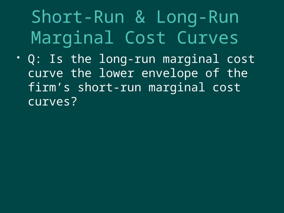
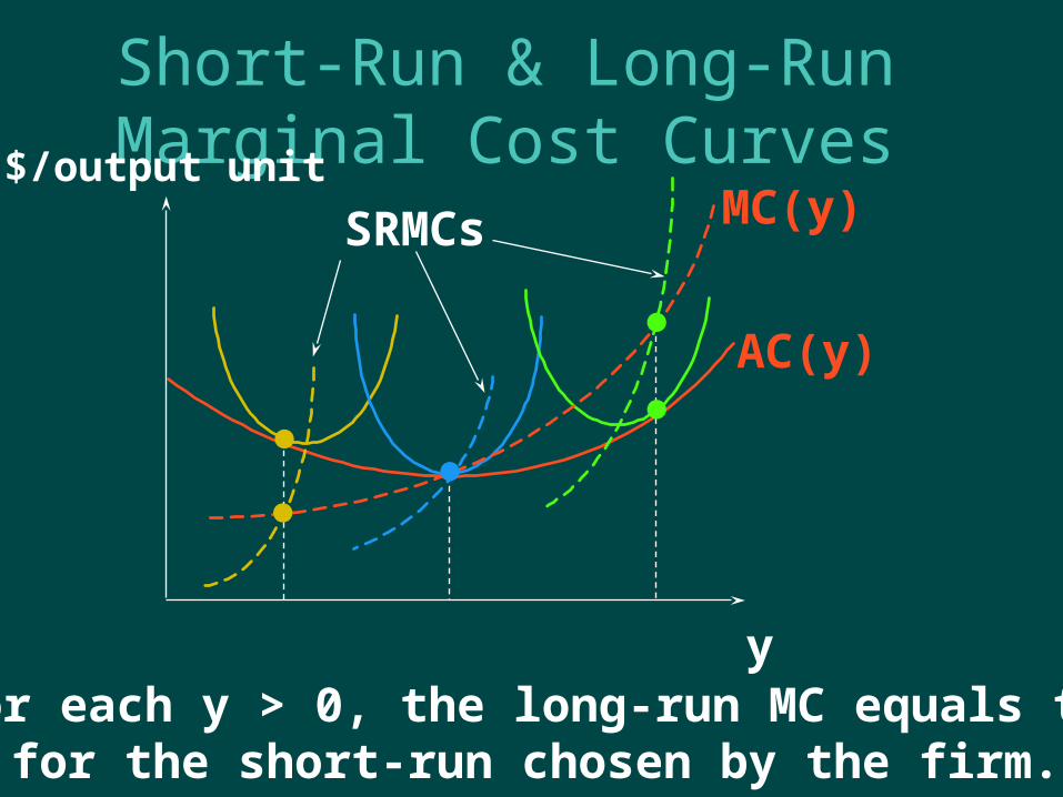
Short-Run & Long-Run Marginal Cost Curves
Q: Is the long-run marginal cost curve the lower envelope of the firm’s short-run marginal cost curves?
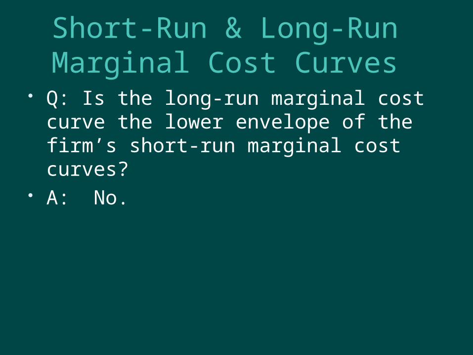
Short-Run & Long-Run Marginal Cost Curves
Q: Is the long-run marginal cost curve the lower envelope of the firm’s short-run marginal cost curves?
A: No.

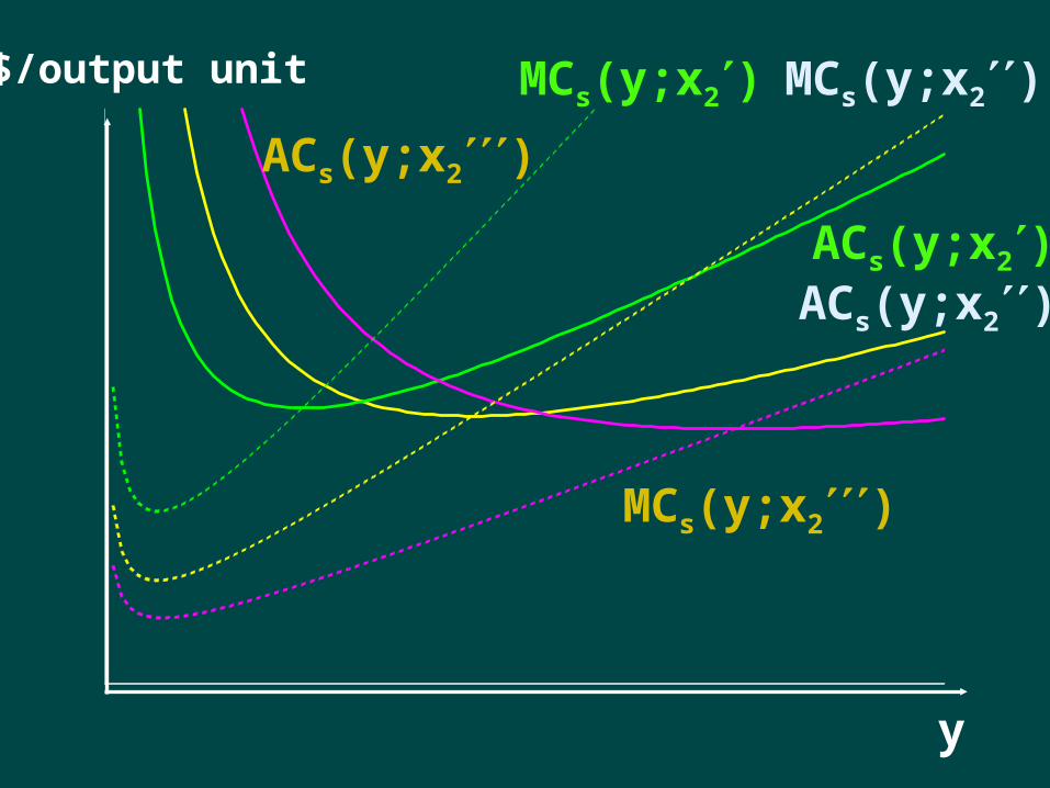
Short-Run & Long-Run Marginal Cost Curves
The firm’s three short-run average total cost curves are ...

y
$/output unit
ACs(y;x2)
ACs(y;x2)
ACs(y;x2)
y
$/output unit
ACs(y;x2)
ACs(y;x2)ACs(y;x2)
MCs(y;x2) MCs(y;x2)
MCs(y;x2)

y
$/output unit
ACs(y;x2)
ACs(y;x2)ACs(y;x2)
MCs(y;x2) MCs(y;x2)
MCs(y;x2)AC(y)

y
$/output unit
ACs(y;x2)
ACs(y;x2)ACs(y;x2)
MCs(y;x2) MCs(y;x2)
MCs(y;x2)AC(y)

y
$/output unit
ACs(y;x2)
ACs(y;x2)ACs(y;x2)
MCs(y;x2) MCs(y;x2)
MCs(y;x2)
MC(y), the long-run marginalcost curve.

Short-Run & Long-Run Marginal Cost Curves
For any output level y > 0, the long-run marginal cost of production equals to the short-run marginal cost of output chosen by the firm , that is,
LRMC(y) = SRMC(y)

Short-Run & Long-Run Marginal Cost Curves
This is always true,
So for the continuous case, where x2 can be fixed at any value of zero or more, the relationship between the long-run marginal cost and all of the short-run marginal costs is ...

Short-Run & Long-Run Marginal Cost Curves
AC(y)
$/output unit
y
SRACs

Short-Run & Long-Run Marginal Cost Curves
AC(y)
$/output unit
y
SRMCs
Short-Run & Long-Run Marginal Cost Curves
AC(y)
MC(y)$/output unit
y
SRMCs
For each y > 0, the long-run MC equals theMC for the short-run chosen by the firm.
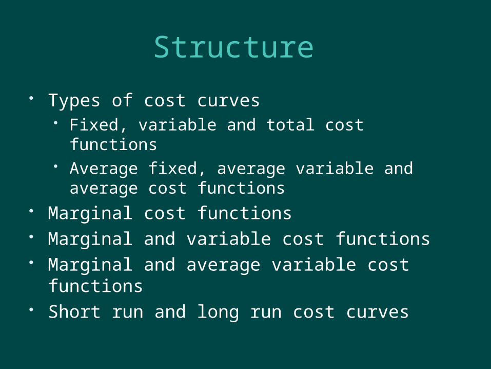
Structure
Types of cost curves Fixed, variable and total cost functions Average fixed, average variable and average
cost functions Marginal cost functions Marginal and variable cost functions Marginal and average variable cost functions Short run and long run cost curves

总成本: TFC、TVC、TC 平均成本:AVC、AFC、AC 边际成本:MC
0
C
Q
TFC
总不变成本曲线Q0
C
TVC
总可变成本曲线
TFC0 Q
C
TC
总成本曲线
AFC
0 Q
C
平均不变成本曲线
MC
0 Q
C
边际成本曲线
AC
0 Q
C
平均总成本曲线
AVC
0 Q
C
平均可变成本曲线
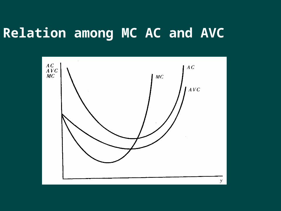
Relation among MC AC and AVC

练习 对于生产函数 ,有两种可变投入 K 、 L ,资本的租赁
价格为 1 元,劳动的工资为 1 元,固定投入为 1000 元。 1 )写出成本曲线。 2 )计算 AC, AVC, AFC, MC 3 )计算 minAC 和 minAVC 时的 AC,AVC,y 。
1/ 4 1/ 4y k L
'( ) 10002 ( ) 4
( ) 10002
C yAC y MC C y y
y y
TVC y FAVC y AFC
y y y
10002)( 2 yyc ( ) 1000min{ 2 }
10 5 40 5 20 5
( )min{ 2 }
0 . 0
C yAC y
y y
y AC AVC
TVC yAVC y
y
y AC does not exist AVC

练习 假设某企业A的生产函数为: 另一家企业B的生产函数为: 其中 y 为产量,K和L分别为资本和劳动的投入量。
a . 如果两家企业使用同样多的资本和劳动,哪一家企业的产量大?
b . 如果资本的投入限于9单位,而劳动的投入没有限制,哪家企业劳动的边际产量更大?
21
21
10 KLyA 52
53
10 KLyB
Related Documents


