Cost 2

Cost theory

By DANIYAL KHANPRESENTED TO

SIR AZEEM BHATTI

The Meaning of Costs

Opportunity costs meaning of opportunity cost

examples

Measuring a firm’s opportunity costs factors not owned by the firm: explicit costs

factors already owned by the firm: implicit costs

Costs

Short run – Diminishing marginal returns results from adding successive quantities of variable factors to a fixed factor

Long run – Increases in capacity can lead to increasing, decreasing or constant returns to scale

Costs

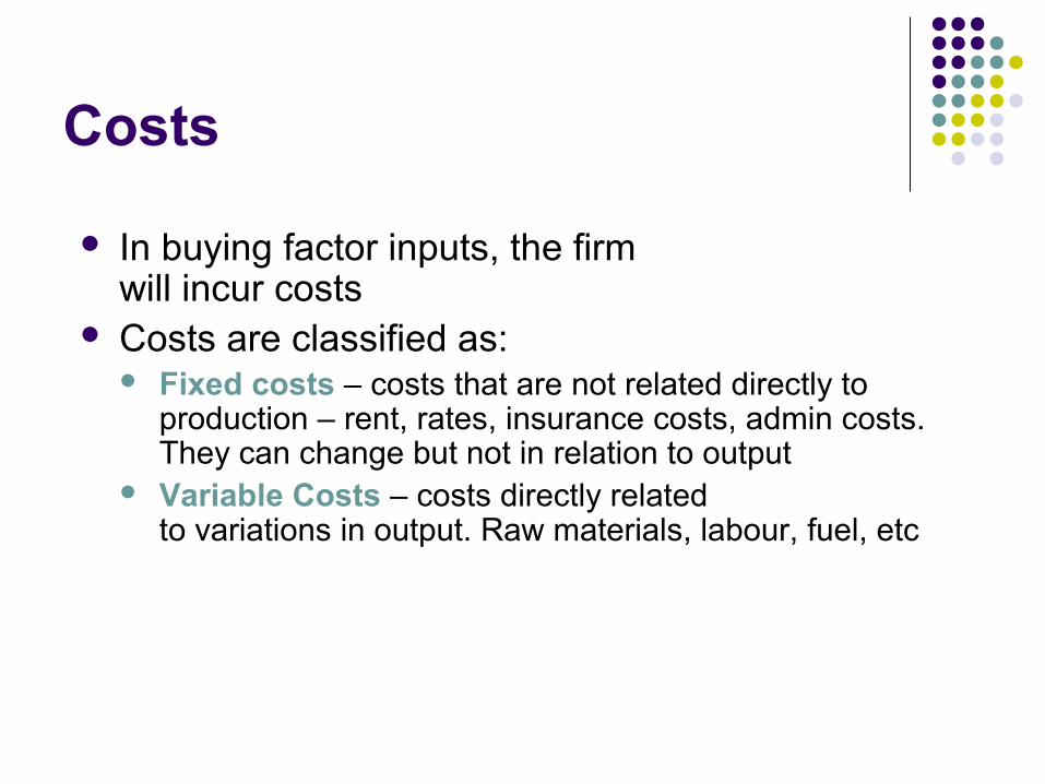
In buying factor inputs, the firm will incur costs

Costs are classified as: Fixed costs – costs that are not related directly to

production – rent, rates, insurance costs, admin costs. They can change but not in relation to output

Variable Costs – costs directly related to variations in output. Raw materials, labour, fuel, etc

Costs

Total Cost - the sum of all costs incurred in production

TC = FC + VC Average Cost – the cost per unit

of output AC = TC/Output

Marginal Cost – the cost of one more or one fewer units of production

MC = TCn – TCn-1 units

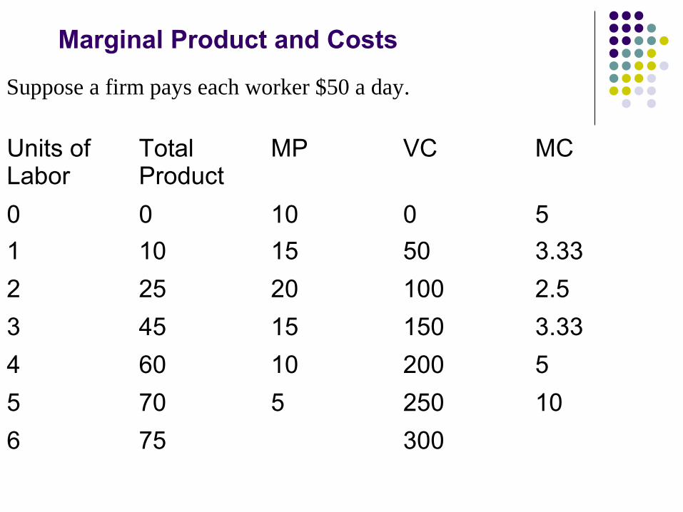
Marginal Product and Costs

Suppose a firm pays each worker $50 a day.

Units of Labor

Total Product

MP VC MC

0 0 10 0 5

1 10 15 50 3.33

2 25 20 100 2.5

3 45 15 150 3.33

4 60 10 200 5

5 70 5 250 10

6 75 300

A Firm’s Short Run Costs

Average Costs

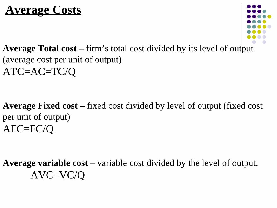
Average Total cost – firm’s total cost divided by its level of output (average cost per unit of output) ATC=AC=TC/Q

Average Fixed cost – fixed cost divided by level of output (fixed cost per unit of output)AFC=FC/Q

Average variable cost – variable cost divided by the level of output.AVC=VC/Q

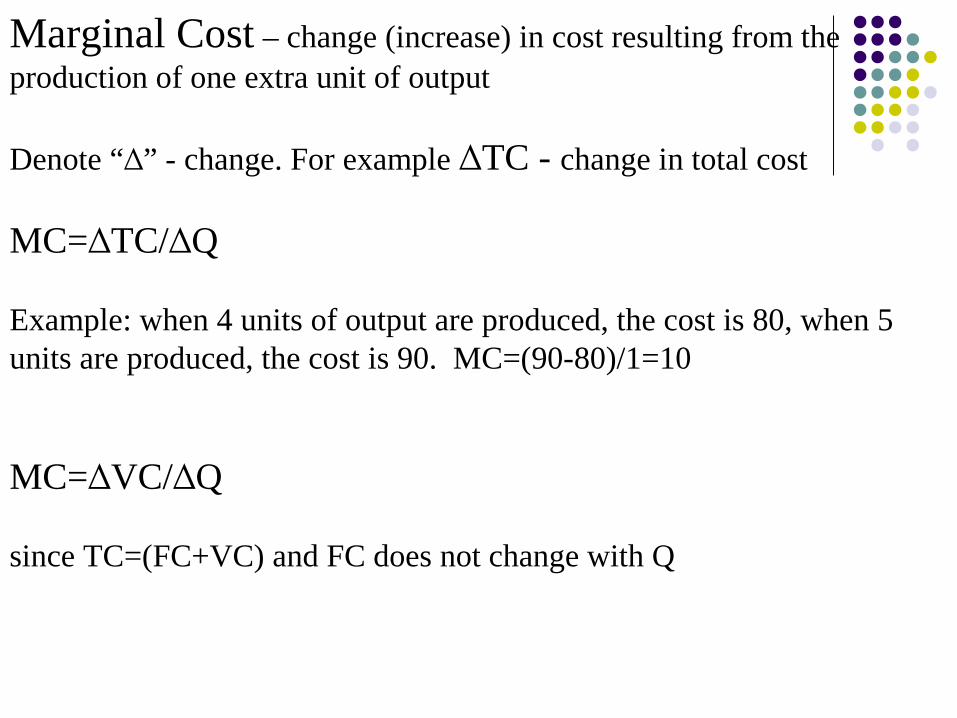
Marginal Cost – change (increase) in cost resulting from the production of one extra unit of output

Denote “ ” - change. For example ∆ TC - ∆ change in total cost

MC= TC/ Q∆ ∆

Example: when 4 units of output are produced, the cost is 80, when 5 units are produced, the cost is 90. MC=(90-80)/1=10

MC= VC/ Q∆ ∆

since TC=(FC+VC) and FC does not change with Q

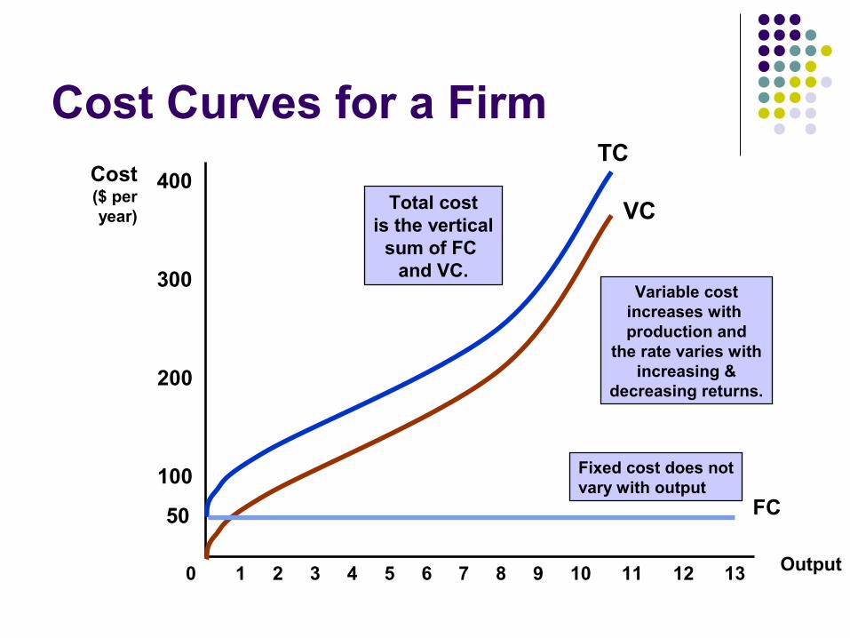
Cost Curves for a Firm

Output

Cost($ peryear)

100

200

300

400

0 1 2 3 4 5 6 7 8 9 10 11 12 13

VC

Variable costincreases with production and

the rate varies withincreasing &

decreasing returns.

TC

Total costis the vertical

sum of FC and VC.

FC50

Fixed cost does notvary with output

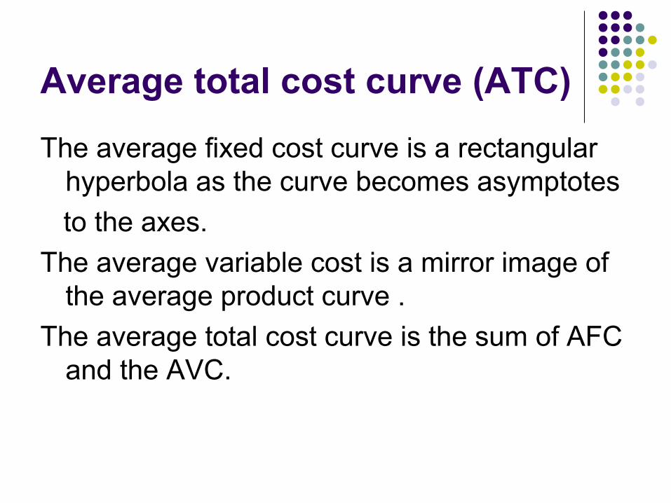
Average total cost curve (ATC)

The average fixed cost curve is a rectangular hyperbola as the curve becomes asymptotes

to the axes.

The average variable cost is a mirror image of the average product curve .

The average total cost curve is the sum of AFC and the AVC.

When both the curves are falling, the ATC which is the sum of both is also falling.

When AVC starts to rise, the average fixed cost curve falls faster and hence the sum falls. Beyond a point, the rise in AVC is more than the fall in AFC and their sum rises.

Hence the ATC is an U shaped curve

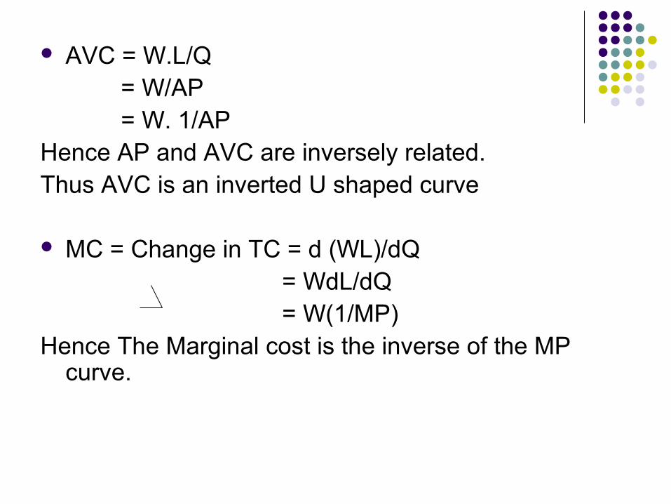
AVC = W.L/Q = W/AP = W. 1/APHence AP and AVC are inversely related.Thus AVC is an inverted U shaped curve

MC = Change in TC = d (WL)/dQ = WdL/dQ = W(1/MP)Hence The Marginal cost is the inverse of the MP

curve.

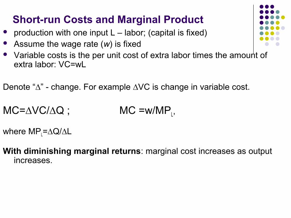
Short-run Costs and Marginal Product production with one input L – labor; (capital is fixed) Assume the wage rate (w) is fixed Variable costs is the per unit cost of extra labor times the amount of

extra labor: VC=wL

Denote “∆” - change. For example ∆VC is change in variable cost.

MC=∆VC/∆Q ; MC =w/MPL,

where MPL=∆Q/∆L

With diminishing marginal returns: marginal cost increases as output increases.

figOutput (Q)

Co

sts

(£)

MC

x

Average and marginal costs

Diminishing marginalreturns set in here

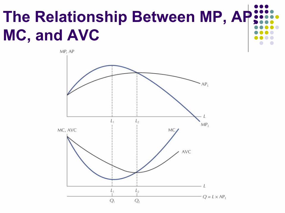
The Relationship Between MP, AP, MC, and AVC

figOutput (Q)

Co

sts

(£)

AFC

AVC

MC

x

AC

z

y

Average and marginal costs

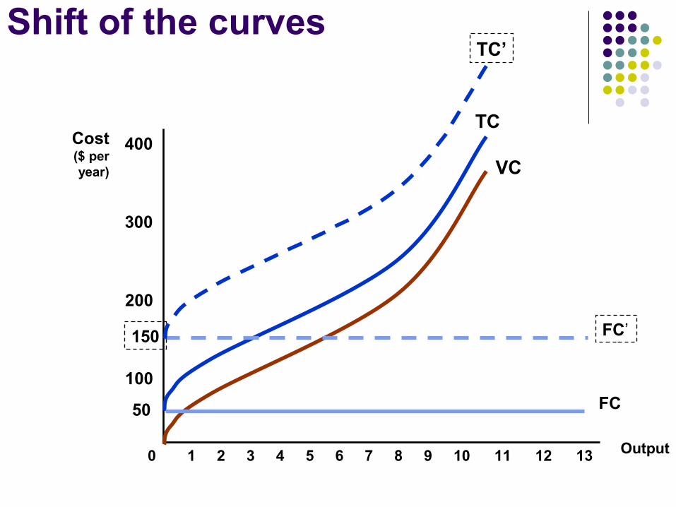
Shift of the curves

Output

Cost($ peryear)

100

200

300

400

0 1 2 3 4 5 6 7 8 9 10 11 12 13

VC

TC

FC50

FC’150

TC’

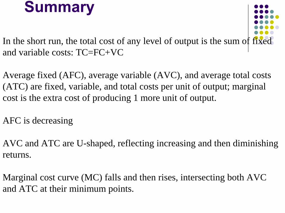
Summary

In the short run, the total cost of any level of output is the sum of fixedand variable costs: TC=FC+VC

Average fixed (AFC), average variable (AVC), and average total costs (ATC) are fixed, variable, and total costs per unit of output; marginal cost is the extra cost of producing 1 more unit of output.

AFC is decreasing

AVC and ATC are U-shaped, reflecting increasing and then diminishingreturns.

Marginal cost curve (MC) falls and then rises, intersecting both AVC and ATC at their minimum points.

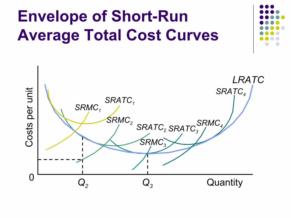
The Envelope Relationship

In the long run all inputs are flexible, while in the short run some inputs are not flexible.

As a result, long-run cost will always be less than or equal to short-run cost.

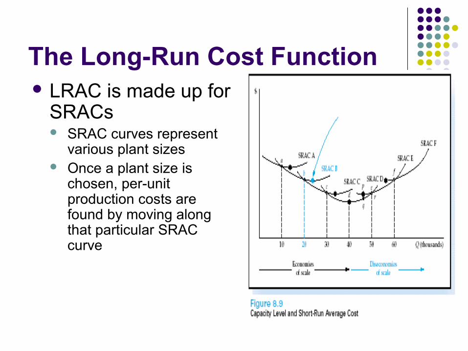
The Long-Run Cost Function LRAC is made up for

SRACs SRAC curves represent

various plant sizes Once a plant size is

chosen, per-unit production costs are found by moving along that particular SRAC curve

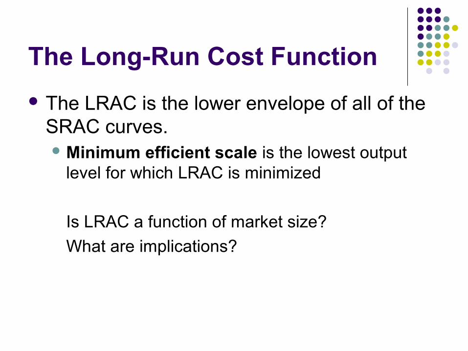
The Long-Run Cost Function

The LRAC is the lower envelope of all of the SRAC curves. Minimum efficient scale is the lowest output

level for which LRAC is minimized

Is LRAC a function of market size?

What are implications?

The Envelope Relationship

The envelope relationship explains that:

At the planned output level, short-run average total cost equals long-run average total cost.

At all other levels of output, short-run average total cost is higher than long-run average total cost.

fig

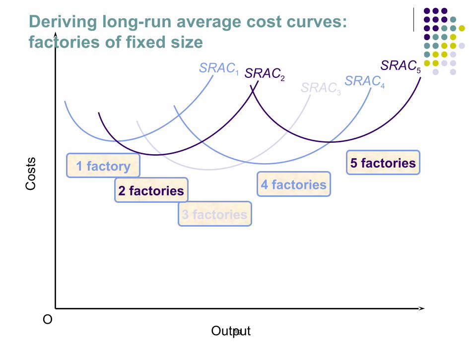
Deriving long-run average cost curves: factories of fixed size

SRAC3

Cos

ts

OutputO

SRAC4

SRAC5

5 factories

4 factories

3 factories

2 factories

1 factory

SRAC1 SRAC2

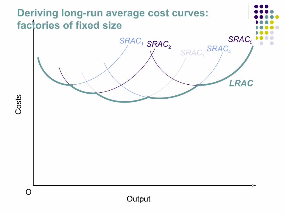
fig

SRAC1

SRAC3

SRAC2 SRAC4

SRAC5

LRAC

Cos

ts

OutputO

Deriving long-run average cost curves: factories of fixed size

Cos

ts p

er u

nit

0 Quantity

SRATC2 SRATC3

SRATC4

LRATC

SRATC1SRMC1

SRMC2

SRMC3

SRMC4

Q2 Q3

Envelope of Short-Run Average Total Cost Curves

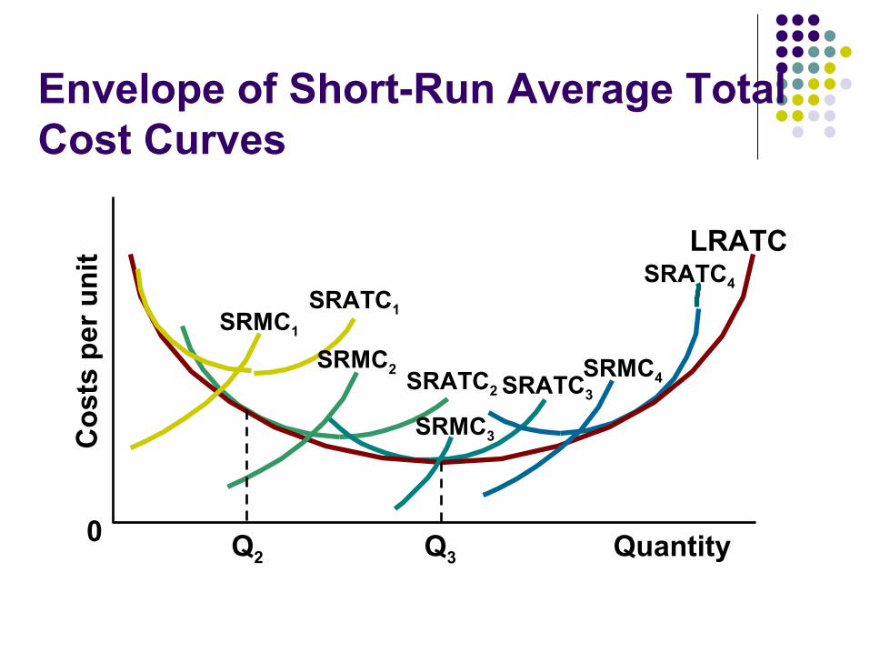
Envelope of Short-Run Average Total Cost Curves

Co

sts

per

un

it

0 Quantity

SRATC2 SRATC3

SRATC4

LRATC

SRATC1SRMC1

SRMC2

SRMC3

SRMC4

Q2 Q3

The Learning Curve

Measures the percentage decrease in additional labor cost each time output doubles. An “80 percent” learning

curve implies that the labor costs associated with the incremental output will decrease to 80% of their previous level.

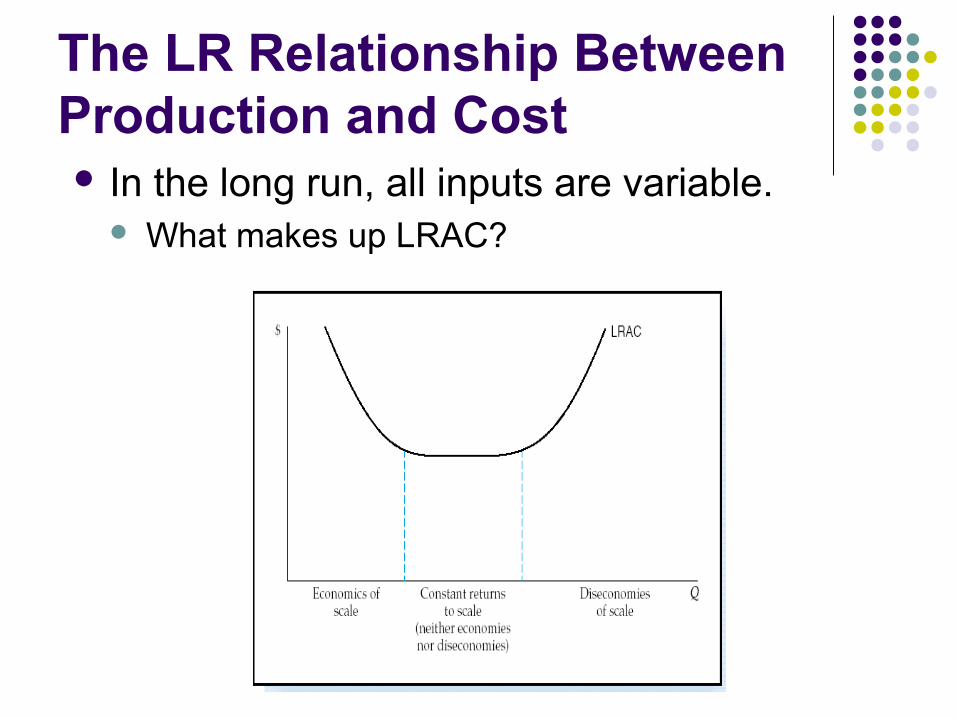
The LR Relationship Between Production and Cost In the long run, all inputs are variable.

What makes up LRAC?

Production in the Long run

Economies of scale specialisation & division of labour indivisibilities container principle greater efficiency of large machines by-products multi-stage production organisational & administrative economies financial economies

Production in the Long run

Diseconomies of scale managerial diseconomies effects of workers and industrial relations risks of interdependencies

External economies of scale Location

balancing the distance from suppliers and consumers

importance of transport costs Ancillary industries-by products

Internal economies and diseconomies

affect the shape of the LAC External Economies affect the position of the

LAC External Diseconomies may cause increase

in prices of the factors of production

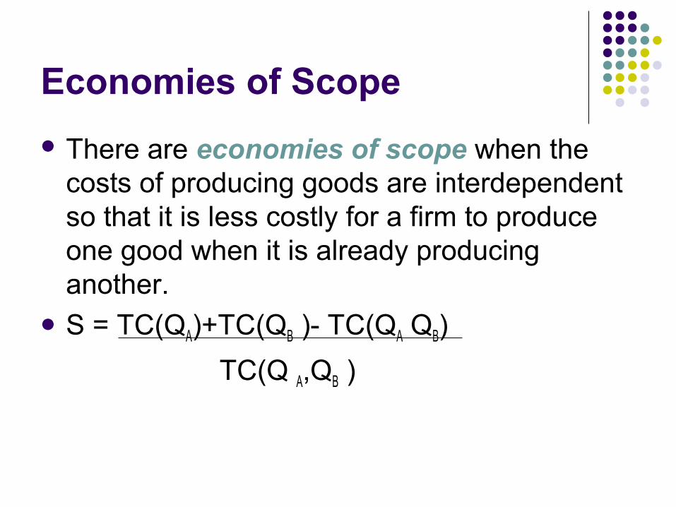
Economies of Scope

There are economies of scope when the costs of producing goods are interdependent so that it is less costly for a firm to produce one good when it is already producing another.

S = TC(QA)+TC(QB )- TC(QA QB)

TC(Q A,QB )

Economies of Scope

Firms look for both economies of scope and economies of scale.

Economies of scope play an important role in firms’ decisions of what combination of goods to produce.

Summary

An economically efficient production process must be technically efficient, but a technically efficient process may not be economically efficient.

The long-run average total cost curve is U-shaped because economies of scale cause average total cost to decrease; diseconomies of scale eventually cause average total cost to increase.

Summary

Marginal cost and short-run average cost curves slope upward because of diminishing marginal productivity.

The long-run average cost curve slopes upward because of diseconomies of scale.

The envelope relationship between short-run and long-run average cost curves shows that the short-run average cost curves are always above the long-run average cost curve.

Summary

Marginal cost and short-run average cost curves slope upward because of diminishing marginal productivity.

The long-run average cost curve slopes upward because of diseconomies of scale.

The envelope relationship between short-run and long-run average cost curves shows that the short-run average cost curves are always above the long-run average cost curve.

Summary

Marginal cost and short-run average cost curves slope upward because of diminishing marginal productivity.

The long-run average cost curve slopes upward because of diseconomies of scale.

The envelope relationship between short-run and long-run average cost curves shows that the short-run average cost curves are always above the long-run average cost curve.

Revenue

Total revenue – the total amount received from selling a given output

TR = P x Q Average Revenue – the average amount

received from selling each unit AR = TR / Q

Marginal revenue – the amount received from selling one extra unit of output

MR = TRn – TR n-1 units