Cosmology An Introduction

Cosmology An Introduction

Ricardo Chavez Murillo

Instituto de Radioastronomıa y AstrofısicaUniversidad Nacional Autonoma de MexicoOctober 2020

ii

Contents

Preface v

List of Symbols viii

1 Introduction 1

2 The Expanding Universe 3

2.1 Cosmology Basics . . . . . . . . . . . . . . . . . . . . . . . . . . . . . . . . . 5

2.1.1 Observational toolkit . . . . . . . . . . . . . . . . . . . . . . . . . . . 8

2.1.2 Growth of structure . . . . . . . . . . . . . . . . . . . . . . . . . . . 10

2.2 Empirical Evidence . . . . . . . . . . . . . . . . . . . . . . . . . . . . . . . . 11

2.2.1 Cosmic microwave background . . . . . . . . . . . . . . . . . . . . . 11

2.2.2 Large-scale structure . . . . . . . . . . . . . . . . . . . . . . . . . . . 14

2.2.3 Current supernovae results . . . . . . . . . . . . . . . . . . . . . . . 15

2.3 Theoretical Landscape . . . . . . . . . . . . . . . . . . . . . . . . . . . . . . 18

2.3.1 The cosmological constant . . . . . . . . . . . . . . . . . . . . . . . . 19

2.3.2 Dark energy theories . . . . . . . . . . . . . . . . . . . . . . . . . . . 22

2.3.3 Modified gravity theories . . . . . . . . . . . . . . . . . . . . . . . . 23

2.4 Probes of Cosmic Acceleration . . . . . . . . . . . . . . . . . . . . . . . . . 24

2.4.1 Type Ia supernovae . . . . . . . . . . . . . . . . . . . . . . . . . . . 24

2.4.2 Galaxy clusters . . . . . . . . . . . . . . . . . . . . . . . . . . . . . . 25

2.4.3 Baryon acoustic oscillations . . . . . . . . . . . . . . . . . . . . . . . 25

2.4.4 Weak gravitational lensing . . . . . . . . . . . . . . . . . . . . . . . . 26

2.4.5 H ii galaxies . . . . . . . . . . . . . . . . . . . . . . . . . . . . . . . 26

2.5 Summary . . . . . . . . . . . . . . . . . . . . . . . . . . . . . . . . . . . . . 27

Appendices 31

A Cosmological Field Equations 31

A.1 The General Relativity Field Equations . . . . . . . . . . . . . . . . . . . . 31

A.2 The Euler-Lagrange Equations . . . . . . . . . . . . . . . . . . . . . . . . . 31

iii

Contents

A.3 Variational Method for Geodesics . . . . . . . . . . . . . . . . . . . . . . . . 32A.4 Application to the FRW Metric . . . . . . . . . . . . . . . . . . . . . . . . . 33A.5 Obtaining the Ricci Tensor . . . . . . . . . . . . . . . . . . . . . . . . . . . 35A.6 The Energy-Momentum Tensor . . . . . . . . . . . . . . . . . . . . . . . . . 36A.7 The Cosmological Field Equations . . . . . . . . . . . . . . . . . . . . . . . 37

B The Cosmic Distance Ladder 39B.1 Kinematic Methods to Distance Determinations . . . . . . . . . . . . . . . . 39

B.1.1 Trigonometric parallax . . . . . . . . . . . . . . . . . . . . . . . . . . 40B.1.2 The moving-cluster method . . . . . . . . . . . . . . . . . . . . . . . 41

B.2 Primary Distance Indicators . . . . . . . . . . . . . . . . . . . . . . . . . . . 42B.2.1 Cepheids . . . . . . . . . . . . . . . . . . . . . . . . . . . . . . . . . 42B.2.2 Tip of the red giant branch method . . . . . . . . . . . . . . . . . . 44

B.3 Secondary Distance Indicators . . . . . . . . . . . . . . . . . . . . . . . . . . 44B.3.1 Type Ia supernovae . . . . . . . . . . . . . . . . . . . . . . . . . . . 44B.3.2 Tully-Fisher relation . . . . . . . . . . . . . . . . . . . . . . . . . . . 45B.3.3 Faber-Jackson relation . . . . . . . . . . . . . . . . . . . . . . . . . . 46

C Statistical Techniques in Cosmology 47C.1 Bayes Theorem and Statistical Inference . . . . . . . . . . . . . . . . . . . . 47C.2 Chi-square and Goodness of Fit . . . . . . . . . . . . . . . . . . . . . . . . . 48C.3 Likelihood . . . . . . . . . . . . . . . . . . . . . . . . . . . . . . . . . . . . . 49C.4 Fisher Matrix . . . . . . . . . . . . . . . . . . . . . . . . . . . . . . . . . . . 49C.5 Monte Carlo Methods . . . . . . . . . . . . . . . . . . . . . . . . . . . . . . 50

List of Figures 51

List of Tables 53

References 55

iv

Preface

The terms ‘cosmological constant’, ‘dark energy’ and ‘modified gravity’ have been remain-ders of our incomplete understanding of the “physical reality”. Our comprehension hasbeen hampered by incomplete and biased data sets and the consequent theoretical overcharged speculation.

Knowledge is constructed progressively, harsh and lengthy battles between proud the-oretical systems, between judgements, must be fought before a glimpse of certainty can beacquired. However, sometimes an apparently tractable petit problem has been enough todemolish the noblest system.

The cosmic acceleration, detected at the end of the 1990s, could be one of this classof problems that are the key to a new view of reality. First of all, this problem is relatedto many fields in physics, crossing from gravitation to quantum field theory and to theunknown in the embodiment of quantum gravity with its multiple flavours (e.g. stringtheory, loop quantum gravity, twistor theory, ...). Even more, the quest for a theoreticalaccount of the observed acceleration has given an enormous impetus to the search foralternative theories of gravity.

The theoretical explanations for the cosmic acceleration are many and diverse, first ofall we have the cosmological constant as a form of vacuum energy, then we are faced witha multitude of models in which its origin is explained by means of a substance with anexotic equation of state, and finally we encounter explanations based on modifications ofthe theory of general relativity.

The fact is that the current empirical data is not enough to discriminate between thegreat number of theoretical models, and therefore if we want to eventually decide on whichis the best model we will need more and accurate data.

v

Contents

vi

List of Symbols

We have attempted to keep the basic notation as standard as possible. In general, thenotation is defined at its first occurrence in the text. The signature of the metric is assumedto be (+,−,−,−) and the speed of light, c, is taken to be equal to 1 throughout this work,unless otherwise specified. Throughout this work the Einstein summation convention isassumed. Note that throughout this work the subscript 0 denotes a parameter’s presentepoch value, unless otherwise specified.

2 The D’Alembert operator.

χ The comoving distance.

χ2 The Chi-square merit function.

δk The perturbations to the mass-energy density decomposed into their Fourier modes.

Γabc The metric connection coefficients or Christoffel symbols.

κ The Einstein’s gravitational constant.

Λ The cosmological constant.

L The Lagrangian density or the likelihood estimator.

µ The distance modulus.

Ω The mass-energy density nomarlized to the present ρc value.

ρ The mass-energy density.

ρc The critical density (that required for the Universe to have a flat spatial geometry).

σ The velocity dispersion from the emission-line width.

a(t) The cosmic scale factor.

cs The sound speed.

vii

List of Symbols

DA The angular distance.

DL The luminosity distance.

DM The proper distance.

dV The comoving volume element.

f The flux.

Gµν The Einstein tensor.

gµν The metric.

H The Hubble parameter.

h The dimensionless Hubble parameter.

L The luminosity.

Mz The H ii galaxies distance indicator.

p The pressure.

q(t) The deceleration parameter .

R The Ricci scalar.

Rµν The Ricci tensor.

Rcurv The curvature radius.

Rc The core radius.

S The action.

s The scale of acoustic oscillations.

t(z) The cosmological time.

Tµν The stress-energy tensor.

EW,W The line equivalent width.

w The equation of state parameter.

z The redshift.

viii

Chapter 1

Introduction

“Begin at the beginning,” the King said gravely,“and go on till you come to the end: then stop.”

— L. Carroll, Alice in Wonderland

Our current understanding of the cosmological evidence shows that our Universe is homo-geneous on the large-scale, spatially flat and in accelerated expansion; it is composed

of baryons, some sort of cold dark matter and a component which acts as having a negativepressure (dubbed ’dark energy’ or ’cosmological constant’). The Universe underwent aninflationary infancy of extremely rapid growth, followed by a phase of gentler expansiondriven initially by its relativistic and then by its non-relativistic contents but by now itsevolution is governed by the dark energy component (e.g. Ratra & Vogeley, 2008; Frieman,Turner & Huterer, 2008).

The observational evidence for dark energy was presented in 1998 when two teamsstudying type Ia supernovae (SNe Ia), the Supernova Cosmology Project and the High-zSupernova Search, found independently that these objects were further away than expectedin a Universe without a cosmological constant (Riess et al., 1998; Perlmutter et al., 1999).Since then measurements of cosmic microwave background (CMB) anisotropy (e.g. Jaffeet al., 2001; Pryke et al., 2002; Spergel et al., 2007; Planck Collaboration et al., 2013) andof large-scale structure (LSS) (e.g. Tegmark et al., 2004; Seljak et al., 2005), in combinationwith independent Hubble relation measurements (Freedman et al., 2001), have confirmedthe accelerated expansion of the Universe.

The accumulated evidence implies that nearly 70% of the total mass-energy of theUniverse is composed of this mysterious dark energy; for which its nature is still largelyunknown. Possible candidates of the cause of the accelerated expansion are Einstein’scosmological constant, which implies that the dark energy component is constant in timeand uniform in space (Carroll, 2001); or it could be that the dark energy is an exotic formof matter with a time dependent equation of state (e.g. Peebles & Ratra, 2003; Copeland,

1

Chapter 1. Introduction

Sami & Tsujikawa, 2006); or since the range of validity of General Relativity (GR) islimited, an extended gravitational theory is needed (e.g. Joyce et al., 2014).

From the previous discussion we can see that understanding the nature of dark energyis of paramount importance and it could have deep implications for fundamental physics;it is thus of no surprise that this problem has been called out prominently in recent policyreports (Albrecht et al., 2006; Peacock et al., 2006) where extensive experimental programsto explore dark energy have been put forward.

To the present day, the cosmic acceleration has been traced directly only by means ofSNe Ia and at redshifts, z ∼ 1, a fact which implies that it is of great importance to usealternative geometrical probes at higher redshifts in order to verify the SNe Ia results andto obtain more stringent constrains in the cosmological parameters solution space, withthe final aim of discriminating among the various theoretical alternatives that attempt toexplain the accelerated expansion of the Universe (cf. Suyu et al., 2012).

2

Chapter 2

The Expanding Universe

We are to admit no more causes of natural thingsthan such as are both true and sufficient to explaintheir appearances.

— I. Newton, Rules of Reasoning in Philosophy :Rule I

The current accepted cosmological model explains the history of the Universe as a suc-cession of epochs characterised by their expansion rates. The Universe expansion rate

has changed as one of its energy components dominates over all others. Near the beginningof time around 10−36 seconds after the ‘big bang’, the dominant component is the so called‘inflaton’ field and the Universe expands exponentially, then after a reheating process, thedominant component is radiation followed by dark matter and at those epochs the ex-pansion of the universe decelerates. Now the Universe is again in a phase of acceleratedexpansion and we call ‘dark energy’ the dominant component that causes it.

Our growing comprehension of the expanding Universe picture has advanced as newdata has been accumulating through the technological improvements that have revolu-tionised astronomy during the past century. The first glimpse of the Universe expansionwas obtained using ground based optical spectroscopy (Hubble, 1929), now the availabledata spans essentially all the electromagnetic spectrum, all kinds of astronomical techniquesand is obtained through ground as well as space borne observations.

Through time different tracers have been used to measure the expansion rate, initiallyextragalactic Cepheids, now Supernovae Ia (SNe Ia), the Cosmic Microwave Background(CMB) and also galaxies. Even so, our current knowledge is insufficient to determine thenature of ‘dark energy’.

The cause of the cosmic acceleration is one of the most intriguing problems in allphysics. In one form or another it is related to gravitation, high energy physics, extradimensions, quantum field theory and even more exotic areas of physics, as quantum gravity

3

Chapter 2. The Expanding Universe

or worm holes. However, we still know very little regarding the mechanism that drives theaccelerated expansion of the Universe.

With the recent confirmation of the existence of the Higgs boson, the plot thickenseven more. The electroweak phase transition generated by the Higgs potential induces anon vanishing contribution to the vacuum energy at the classical level that is blatantlyin discordance with the accepted value for the cosmological constant in the ‘concordance’(ΛCDM) cosmological model, thus leaving us with an embarrassingly large fine tuningproblem (cf. Sola, 2013).

Due to the lack of a fundamental physical theory explaining the accelerated expansion,there have been many theoretical speculations about the nature of dark energy (e.g. Cald-well & Kamionkowski, 2009; Frieman, Turner & Huterer, 2008); furthermore and mostimportantly, the current observational/experimental data is not adequate to distinguishbetween the many adversary theoretical models.

Essentially one can probe dark energy by one or more of the following methods:

• Geometrical probes of the cosmic expansion, which are directly related to the metriclike distances and volumes.

• Growth probes related to the growth rate of the matter density perturbations.

The existence of dark energy was first inferred from a geometrical probe, the redshift-distance relation of SNe Ia (Riess et al., 1998; Perlmutter et al., 1999); this method con-tinues to be the preeminent way to probe directly the cosmic acceleration. The recentUnion2.1 (Suzuki et al., 2012), SNLS3 (Conley et al., 2011) and PS1 (Rest et al., 2013)compilations of SNe Ia data are consistent with a cosmological constant, although theresults, within reasonable statistical uncertainty, also agree with many dynamical dark-energy models (Shafer & Huterer, 2014). It is therefore of great importance to trace theHubble function to higher redshifts than currently probed, since at higher redshifts thedifferent models deviate significantly from each other (Plionis et al., 2011).

In this chapter we will explore the Cosmic Acceleration issue; the first section is devotedto a general account of the basics of theoretical and observational cosmology, in the secondsection we present a brief outlook of the observational evidence which supports the cosmicacceleration; later we will survey some of the theoretical explanations of the acceleratingexpansion and finally we will overview some probes used to test the Universe expansion.

Finally, a few words of caution regarding the terminology used. Through this chapterwe will be using the term dark energy as opposed to cosmological constant, in the senseof a time-evolving cause of the cosmic acceleration. However, in later chapters we will useonly the term dark energy since we consider it as the most general model, of which thecosmological constant is (mathematically) a particular case, while it effectively reproducesalso the phenomenology of some modified gravity models.

4

2.1. Cosmology Basics

2.1 Cosmology Basics

The fundamental assumption over which our current understanding of the Universe is con-structed is known as the cosmological principle, which states that the Universe is homoge-neous and isotropic on large-scales. The evidences that sustain the cosmological principleare basically the near-uniformity of the CMB temperature (e.g. Spergel et al., 2003) andthe large-scale distribution of galaxies (e.g. Yadav et al., 2005).

Under the assumption of homogeneity and isotropy, the geometrical properties of space-time are described by the Friedmann-Robertson-Walker (FRW) metric (Robertson, 1935),given by

ds2 = dt2 − a2(t)

[dr2

1− kr2+ r2(dθ2 + sin2 θdφ2)

], (2.1)

where r, θ, φ are spatial comoving coordinates (i.e., where a freely falling particle comesto rest) and t is the time parameter, whereas a(t) is the cosmic scale factor which at thepresent epoch, t0, has a value a(t0) = 1; k is the curvature of the space, such that k = 0corresponds to a spatially flat Universe, k = 1 to a positive curvature (three-sphere) andk = −1 to a negative curvature (saddle as a 2-D analogue). Note that we are using unitswhere the speed of light, c = 1.

From the FRW metric we can derive the cosmological redshift, i.e. the amount that aphoton’s wavelength (λ) increases due to the scaling of the photon’s energy with a(t), withcorresponding definition:

1 + z ≡ λ0

λe=a(t0)

a(t)=

1

a(t), (2.2)

where, z is the redshift, λ0 is the observer’s frame wavelength and λe is the emission’sframe wavelength. Note that throughout this thesis the subscript 0 denotes a parameter’spresent epoch value.

In order to determine the dynamics of the space-time geometry we must solve the GRfield equations for the FRW metric, in the presence of matter, obtaining the cosmologicalfield equations or Friedmann-Lemaıtre equations (for a full derivation see Appendix A):(

a

a

)2

=8πGρ

3− k

a2+

Λ

3, (2.3)

a

a= −4πG

3(ρ+ 3p) +

Λ

3, (2.4)

where ρ is the total energy density of the Universe, p is the total pressure and Λ is thecosmological constant.

In eq.(2.3) we can define the Hubble parameter

H ≡ a

a, (2.5)

5


of which its present value is conventionally expressed as H0 = 100h km s−1 Mpc−1, whereh is the dimensionless Hubble parameter and unless otherwise stated we take a value ofh = 0.743± 0.043 (Chavez et al., 2012; Freedman et al., 2012; Riess et al., 2011; Freedmanet al., 2001; Tegmark et al., 2006).

The time derivative of eq.(2.3) gives:

a =8πG

3

(ρa+

ρa2

2a

)+

Λa

3,

and from the above and eq.(2.4) we can eliminate a to obtain

−4πGa

3

[(ρ+ 3p) + 2

(ρ+

ρa

2a

)]= 0

a

aρ+ 3(ρ+ p) = 0,

which then gives:

ρ+3a

a(ρ+ p) = 0, (2.6)

which is an expression of energy conservation.Equation (2.6) can be written as

d(ρa3)

dt= −3a2ap (2.7)

d(ρa3)

da= −3a2p, (2.8)

and thus:

d(ρia3) = −pida3, (2.9)

where the subscript i runs over all the components of the Universe. Equation (2.9) is theexpanding universe analog of the first law of thermodynamics, dE = −pdV .

If we assume that the different components of the cosmological fluid have an equationof state of the generic form:

pi = wiρi, (2.10)

then from eq.(2.8) we haved(ρia

3)

da= −3wiρia

2, (2.11)

which in the case where the equation of state parameter depends on time, ie., wi(a), thecorresponding density takes the following form:

ρi ∝ exp

−3

∫da

a[1 + wi(a)]

. (2.12)

6


For the particular case where wi is a constant through cosmic time, we have

ρi ∝ a−3(1+wi), (2.13)

where wi ≡ pi/ρi.These last two equations can be written as a function of redshift, definedby the eq.(2.2), as:

ρi ∝ exp

[3

∫ z

0

1 + wi(z′)

1 + z′dz′], (2.14)

ρi ∝ (1 + z)3(1+wi) . (2.15)

For the case of non-relativistic matter (dark matter and baryons), wm = 0 and ρm ∝(1 + z)3, while for relativistic particles (radiation and neutrinos), wr = 1/3 and ρr ∝(1+z)4, while for vacuum energy (cosmological constant), wΛ = −1 and for which we havepΛ = −ρΛ = −Λ/8πG.

In general the dark energy equation of state can be parameterized as (e.g. Plionis et al.,2009)

pw = w(z)ρw, (2.16)

where

w(z) = w0 + w1f(z), (2.17)

with w0 = w(0) and f(z) is an increasing function of redshift, such as f(z) = z/(1 + z)(Chevallier & Polarski, 2001; Linder, 2003; Peebles & Ratra, 2003; Dicus & Repko, 2004;Wang & Mukherjee, 2006).

The so called critical density corresponds to the total energy density of the Universe.From eq.(2.3), where we take the cosmological constant as a cosmic fluid, and the definitionof the Hubble parameter, eq.(2.5), we have that:

ρc ≡3H2

0

8πG= 1.88× 10−29h2 g cm−3 = 8.10× 10−47h2 GeV4 . (2.18)

This parameter provides a convenient mean to normalize the mass-energy densities of thedifferent cosmic components, and we can write:

Ωi =ρi(t0)

ρc, (2.19)

where the subscript i runs over all the different components of the cosmological fluid. Usingthis last definition and eq.(2.14) we can write eq.(2.3) as:

H2(z) = H20

[Ωr(1 + z)4 + Ωm(1 + z)3 + Ωk(1 + z)2 + Ωw exp

(3

∫ z

0

1 + w(z′)

1 + z′dz′)]

,

(2.20)

7


where Ωk has been defined as

Ωk ≡−ka2H2

0

.

By definition we have that Ωr + Ωm + Ωk + Ωw ≡ 1, and as a useful parameter we candefine Ω0 ≡ Ωr + Ωm + Ωw, such that for a positively curved Universe Ω0 > 1 and for anegatively curved Universe Ω0 < 1.

The value of the curvature radius, Rcurv ≡ a/√|k|, is given by

Rcurv =H−1

0√|Ω0 − 1|

, (2.21)

then its characteristic scale or Hubble radius is given by H−10 ≈ 3000h−1 Mpc.

2.1.1 Observational toolkit

In observational cosmology the fundamental observable is the redshift, and therefore it isimportant to express the distance relations in terms of z. The first distance measure tobe considered is the lookback time, i.e. the difference between the age of the Universe atobservation t0 and the age of the Universe, t, when the photons were emitted. From thedefinitions of redshift, eq.(2.2), and the Hubble parameter, eq.(2.5), we have:

dz

dt= − a

a2= −H(z)(1 + z) ,

from which we have:

dt = − dz

H(z)(1 + z), (2.22)

and the lookback time is defined as:

t0 − t =

∫ t0

tdt =

∫ z

0

dz′

H(z′)(1 + z′)=

1

H0

∫ z

0

dz′

(1 + z′)E(z′), (2.23)

where

E(z) =

√Ωr(1 + z)4 + Ωm(1 + z)3 + Ωk(1 + z)2 + Ωw exp

(3

∫ z

0

1 + w(z′)

1 + z′dz′). (2.24)

From the definition of lookback time it is clear that the cosmological time or the timeback to the Big Bang, is given by

t(z) =

∫ ∞z

dz′

(1 + z′)H(z′). (2.25)

8


In the following discussion it will be useful to have an adequate parameterization of theFRW metric (Hobson, Efstathiou & Lasenby, 2005) which is given by:

ds2 = dt2 − a2(t)[dχ2 + S2(χ)(dθ2 + sin2 θdφ2)

],

where the function r = S(χ) is:

S(χ) =

√k−1

sin(χ√k) if k > 0,

χ if k = 0,√|k|−1

sinh(χ√|k|) if k < 0,

(2.26)

We can see that the comoving distance, i.e., that between two free falling particles whichremains constant with epoch, is defined by:

χ =

∫ t0

t

dt

a(t)=

1

H0

∫ z

0

dz′

E(z′). (2.27)

The transverse comoving distance (also called proper distance) is defined as:

DM (t) = a(t)S(χ), (2.28)

At the present time and for the case of a flat model we have, DM = a(t0)χ = χ.The angular distance is defined as the ratio of an object’s physical transverse size to

its angular size, and can be expressed as:

DA =DM

1 + z. (2.29)

Finally, the luminosity distance is defined by means of the relation

f =L

4πD2L

, (2.30)

where f is an observed flux, L is the intrinsic luminosity of the observed object and DL isthe luminosity distance; from which one obtains:

DL = (1 + z)DM = (1 + z)

∫ z

0

dz′

H(z′). (2.31)

The distance modulus of a given cosmic object is defined as:

µ ≡ m−M = 5 log(DL/10 pc) (2.32)

where m and M are the apparent and absolute magnitude of the object, respectively. Ifthe distance, DL, is expressed in Mpc then we have:

µ = 5 logDL + 25 . (2.33)

9


Through this relation and with the use of standard candles, i.e. objects of fixed absolutemagnitude M , we can constrain the different parameters of the cosmological models viathe construction of the Hubble diagram (the magnitude-redshift relation).

The following relation is useful when working with fluxes and luminosities instead ofmagnitudes,

logL = log f + 0.4µ+ 40.08 , (2.34)

where f is the observed flux of the object, L the luminosity and µ the distance modulusas defined in 2.33.

The scale factor can be Taylor expanded around its present value:

a(t) = a(t0)− (t0 − t)a(t0) +1

2(t0 − t)2a(t0)− · · ·

= a(t0)[1− (t0 − t)H(t0)− 1

2(t0 − t)2q(t0)H2(t0)− · · · ]

= 1 +H0(t− t0)− 1

2q0H

20 (t− t0)2 + · · · ,

where the deceleration parameter q(t) is given by

q(t) ≡ − a(t)a(t)

a2(t). (2.35)

From the previous definitions we can write an approximation to the distance-redshift rela-tion as

H0DL = z +1

2(1− q0)z2 + · · · , (2.36)

where we can recognize that for z 1 it can be written as

H0DL ≈ z, (2.37)

which is known as the “Hubble law”.Finally the comoving volume element, as a function of redshift, can be written as:

dV

dzdΩ=S2(χ)

H(z), (2.38)

where Ω is the solid angle.

2.1.2 Growth of structure

The accelerated expansion of the Universe affects the evolution of cosmic structures sincethe expansion rate influences the growth rate of the density perturbations.

The basic assumptions regarding the evolution of structure in the Universe are that thedark matter is composed of non relativistic particles, i.e it is composed of what is called cold

10

2.2. Empirical Evidence

dark matter (CDM), and that the initial spectrum of density perturbations is nearly scaleinvariant, P (k) ∼ kns , where the spectral index is ns ' 1, as it is predicted by inflation.With this in mind, the linear growth of small amplitude, matter density perturbations onlength scales much smaller than the Hubble radius is governed by a second order differentialequation, constructed by linearizing the perturbed equations of motions of a cosmic fluidelement and given by:

δk + 2Hδk − 4πGρmδk = 0, (2.39)

where the perturbations δk ≡ δρm(x, t)/ρm(t) have been decomposed into their Fouriermodes of wave number k. The expansion of the Universe enters through the so-called“Hubble drag” term, 2Hδk. Note that ρm is the mean density.

The growing mode solution of the previous differential equation, in the standard con-cordance cosmological model (wΛ = −1) is given by:

δk(z) ∝ H(z)(5Ωm/2)

∫ ∞z

1 + z′

H3(z′)dz′ . (2.40)

From the previous equation we obtain that, δk(t) is approximately constant during theradiation dominated epoch, grows as a(t) during the matter dominated epoch and againis constant during the cosmic acceleration dominated epoch, in which the growth of linearperturbations effectively freezes.

2.2 Empirical Evidence

The cosmic acceleration was established empirically at the end of the 1990s when twoindependent teams, the Supernova Cosmology Project and the High-z Supernova Search,succeeded in their attempt to measure the supernova Hubble diagram up to relatively highredshifts (z ∼ 1) (Riess et al., 1998; Perlmutter et al., 1999). Surprisingly, both teams foundthat the distant supernovae are ∼ 0.25 mag dimmer that they would be in a deceleratinguniverse, indicating that the cosmic expansion has been accelerating over the past ∼ 7 Gyr(see Figure 2.1).

The cosmic acceleration has been verified by many other probes, and in this sectionwe will briefly review the current evidence on which this picture of the Universe wasconstructed.

2.2.1 Cosmic microwave background

The measurement of the CMB black body spectrum was one of the most important tests ofthe big bang cosmology. The CMB spectrum started being studied by means of balloon androcket borne observations and finally the black body shape of the spectrum was settled inthe 1990s by observations with the FIRAS radiometer at the Cosmic Background Explorer

11


Figure 2.1: Upper panel: Hubble diagram of type Ia supernovae measured by the Supernova Cos-mology Project and the High-z Supernova Team. Lower Panel: Residuals in distance modulusrelative to an open Universe with Ω0 = Ωm = 0.3. Taken from Perlmutter & Schmidt (2003).

Satellite (COBE) (Mather et al., 1990), which also showed that the departures from a pureblackbody were extremely small (δE/E ≤ 10−4) (Fixsen et al., 1996).

The CMB anisotropies provide a vision of the Universe when photons decoupled frombaryons and before structure developed, about 380000 years after the Big Bang. Theangular power spectrum of the CMB temperature anisotropies is dominated by acousticpeaks that arise from gravity-driven sound waves in the photon-baryon fluid. The positionand amplitudes of the acoustic peaks indicate it the Universe is spatially flat or not (seeFigure 2.2). Furthermore, in combination with Large Scale Structure (LSS) or independentH0 measurements, it shows that the matter contributes only about 25% of the criticalenergy density (Hu & Dodelson, 2002). Clearly, a component of missing energy is necessaryto match both results, a fact which is fully consistent with the dark energy being anexplanation of the accelerated expansion.

12


Figure 2.2: Sensitivity of the acoustic temperature spectrum to four fundamental cosmologicalparameters. (a) The curvature as quantified by Ω0. (b) The dark energy as quantified by thecosmological constant ΩΛ (wΛ = −1). (c) The baryon density Ωbh

2. (d) The matter density Ωmh2.

All parameters are varied around a fiducial model with: Ω0 = 1,ΩΛ = 0.65,Ωbh2 = 0.02,Ωmh

2 =0.147, n = 1, zri = 0, Ei = 0. Taken from Hu & Dodelson (2002).

Measurements of the angular power spectrum of the CMB have been carried out inthe last ten years by many experiments (e.g. Jaffe et al., 2001; Pryke et al., 2002; Spergelet al., 2007; Reichardt et al., 2009)]. Figure 2.3 shows a combination of some recent resultswhere the first acoustic peak around l = 200 is clearly seen, which constrain the spatialcurvature of the universe to be very close to null.

The most recent results from the Planck mission (Planck Collaboration et al., 2013) areshown in Figure 2.4. The Planck mission results are consistent with the standard spatially-flat six-parameter ΛCDM cosmology but with a slightly lower value for H0 and a highervalue for Ωm compared with the SNe Ia results. When curvature is included, the PlanckCMB data is consistent with a flat Universe to percent level precision.

Although all these results are consistent with an accelerating expansion of the universe,they alone are not conclusive; other cosmological data, like the independent measurement

13


Figure 2.3: Angular power spectrum measurements of the cosmic microwave background temper-ature fluctuations from the Wilkinson Microwave Anisotropy Probe (WMAP), Boomerang, andthe Arcminute Cosmology Bolometer Array Receiver (ACBAR). Taken from Frieman, Turner &Huterer (2008).

of the Hubble constant, are necessary in order to indicate the cosmic acceleration.

2.2.2 Large-scale structure

The two-point correlation function of galaxies, as a measure of distribution of galaxies onlarge scales, has long been used to provide constrains on various cosmological parameters.The measurement of the correlation function of galaxies from the APM survey excluded,at that time, the standard cold dark matter (CDM) picture (Maddox et al., 1990) and sub-sequently argued in favor of a model with a low density CDM and possibly a cosmologicalconstant (Efstathiou, Sutherland & Maddox, 1990).

The baryonic acoustic oscillations (BAO) leave a characteristic signature in the clus-tering of galaxies, a bump in the two-point correlation function at a scale ∼ 100h−1 Mpcthat can be measured today. Measurements of the BAO signature have been carried out byEisenstein et al. (2005) for luminous red galaxies of the Sloan Digital Sky Survey (SDSS).They find results for the value of Ωmh

2 and the acoustic peak at 100h−1 Mpc scale whichare consistent with the outcome of the CMB fluctuation analyses (see Figure 2.5).

The recent work by Padmanabhan et al. (2012) reanalyses the Eisenstein et al. (2005)sample using an updated algorithm to account for the effects of survey geometry as wellas redshift-space distortions finding similar results, while more recently Anderson et al.

14


Figure 2.4: Angular power spectrum measurements of the cosmic microwave background tempera-ture fluctuations form Planck. The power spectrum at low multipoles (l = 2 − 49) is plotted in alogarithmic multipole scale. Taken from Planck Collaboration et al. (2013).

(2014), using the clustering of galaxies from the SDSS DR11 and in combination with thedata from Planck find best fits of Ωmh

2 = 0.1418± 0.0015 and Ωm = 0.311± 0.009.

2.2.3 Current supernovae results

After the first SNe Ia results were published, concerns were raised about the possibility thatintergalactic extinction or evolutionary effects could be the cause of the observed distantsupernovae dimming (Aguirre, 1999; Drell, Loredo & Wasserman, 2000). Since then anumber of surveys have been conducted which have strengthened the evidence for cosmicacceleration. Observations with the Hubble Space Telescope (HST), have provided highquality light curves (Riess et al., 2007), and observations with ground based telescopes, havepermitted the construction of two large surveys, based on 4 meter class telescopes, the SNLS(Supernova Legacy Survey) (Astier et al., 2006) and the ESSENCE (Equation of State:Supernovae Trace Cosmic Expansion) survey (Miknaitis et al., 2007) with spectroscopic

15


Figure 2.5: Detection of the baryon acoustic peak in the clustering of luminous red galaxies inthe Sloan Digital Sky Survey (Eisenstein et al., 2005). The two-point galaxy correlation functionin redshift space is shown; the inset shows an expanded view with a linear vertical axis. Curvescorrespond to the ΛCDM predictions for Ωmh

2 = 0.12 (dark yellow), 0.13 (red), and 0.14 (blue).The magenta curve shows a ΛCDM model without baryonic acoustic oscillations. Taken fromFrieman, Turner & Huterer (2008).

16


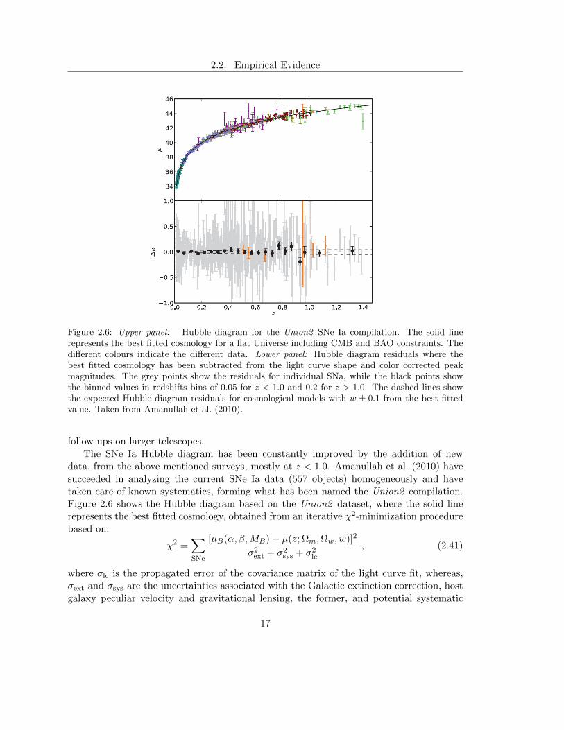
Figure 2.6: Upper panel: Hubble diagram for the Union2 SNe Ia compilation. The solid linerepresents the best fitted cosmology for a flat Universe including CMB and BAO constraints. Thedifferent colours indicate the different data. Lower panel: Hubble diagram residuals where thebest fitted cosmology has been subtracted from the light curve shape and color corrected peakmagnitudes. The grey points show the residuals for individual SNa, while the black points showthe binned values in redshifts bins of 0.05 for z < 1.0 and 0.2 for z > 1.0. The dashed lines showthe expected Hubble diagram residuals for cosmological models with w ± 0.1 from the best fittedvalue. Taken from Amanullah et al. (2010).

follow ups on larger telescopes.

The SNe Ia Hubble diagram has been constantly improved by the addition of newdata, from the above mentioned surveys, mostly at z < 1.0. Amanullah et al. (2010) havesucceeded in analyzing the current SNe Ia data (557 objects) homogeneously and havetaken care of known systematics, forming what has been named the Union2 compilation.Figure 2.6 shows the Hubble diagram based on the Union2 dataset, where the solid linerepresents the best fitted cosmology, obtained from an iterative χ2-minimization procedurebased on:

χ2 =∑SNe

[µB(α, β,MB)− µ(z; Ωm,Ωw, w)]2

σ2ext + σ2

sys + σ2lc

, (2.41)

where σlc is the propagated error of the covariance matrix of the light curve fit, whereas,σext and σsys are the uncertainties associated with the Galactic extinction correction, hostgalaxy peculiar velocity and gravitational lensing, the former, and potential systematic

17


Figure 2.7: Left panel: 68.3 %, 95.4 % and 99.7% confidence regions in the (Ωm,ΩΛ) plane fromSNe, BAO and CMB with systematic errors. Cosmological constant dark energy (w = −1) hasbeen assumed. Right panel: 68.3 %, 95.4 % and 99.7% confidence regions in the (Ωm, w) plane fromSNe, BAO and CMB with systematic errors. Zero curvature and constant w has been assumed.Taken from Amanullah et al. (2010).

errors the later. The observed distance modulus is defined as µB = mcorrB −MB, where MB

is the absolute B-band magnitude and mcorrB = mmax

B + αx1 − βc; furthermore mmaxB , x1

and c are parameters for each supernova that are weighted by the nuisance parameters α,β and MB which are fitted simultaneously with the cosmological parameters (z; Ωm,Ωw, w)which give the model distance modulus µ.

Combining the data from the three probes that have been considered up to now, it ispossible to obtain stronger constraints over the cosmological parameters (see Figure 2.7).

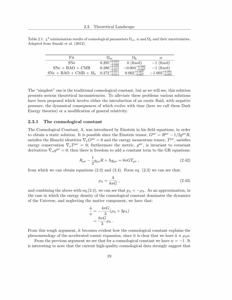
More recently, Suzuki et al. (2012) have added 23 SNe Ia (10 of which are beyond z = 1)to the Union2 compilation to form the Union2.1 dataset. Using this improved catalog ofSNe Ia jointly with BAO and CMB data they obtain even better constraints to the valuesof the cosmological parameters as shown in Table 2.1.

2.3 Theoretical Landscape

The cosmic accelerated expansion has deep consequences for our understanding of thephysical world. From the theoretical side many plausible explanations have been proposed.

18

2.3. Theoretical Landscape

Table 2.1: χ2 minimisation results of cosmological parameters Ωm, w and Ωk and their uncertainties.Adapted from Suzuki et al. (2012).

Fit Ωm Ωk w

SNe 0.295+0.043−0.040 0 (fixed) −1 (fixed)

SNe + BAO + CMB 0.286+0.018−0.017 −0.004+0.006

−0.007 −1 (fixed)

SNe + BAO + CMB + H0 0.272+0.015−0.014 0.002+0.007

−0.007 −1.003+0.091−0.095

The “simplest” one is the traditional cosmological constant, but as we will see, this solutionpresents serious theoretical inconsistencies. To alleviate these problems various solutionshave been proposed which involve either the introduction of an exotic fluid, with negativepressure, the dynamical consequences of which evolve with time (here we call them DarkEnergy theories) or a modification of general relativity.

2.3.1 The cosmological constant

The Cosmological Constant, Λ, was introduced by Einstein in his field equations, in orderto obtain a static solution. It is possible since the Einstein tensor, Gµν = Rµν − 1/2gµνR,satisfies the Bianchi identities ∇νGµν = 0 and the energy momentum tensor, Tµν , satisfiesenergy conservation ∇νTµν = 0; furthermore the metric, gµν , is invariant to covariantderivatives ∇αgµν = 0; then there is freedom to add a constant term to the GR equations:

Rµν −1

2gµνR+ Λgµν = 8πGTµν , (2.42)

from which we can obtain equations (2.3) and (2.4). Form eq. (2.3) we can see that:

ρΛ =Λ

8πG, (2.43)

and combining the above with eq.(2.4), we can see that pΛ = −ρΛ. As an approximation, inthe case in which the energy density of the cosmological constant dominates the dynamicsof the Universe, and neglecting the matter component, we have that:

a

a= −4πG

3(ρΛ + 3pΛ)

=8πG

3ρΛ .

From this rough argument, it becomes evident how the cosmological constant explains thephenomenology of the accelerated cosmic expansion, since it is clear that we have a ∝ ρΛa.

From the previous argument we see that for a cosmological constant we have w = −1. Itis interesting to note that the current high-quality cosmological data strongly suggest that

19


the mechanism behind the cosmic acceleration behaves exactly as a cosmological constant.However, we will show that the Λ-based explanation of the accelerating universe presentsserious theoretical inconsistencies.

From the point of view of modern field theories, the cosmological constant can beexplained as the energy of the vacuum. The possible sources for the vacuum energy arebasically of two kinds: a bare cosmological constant in the general relativity action or theenergy density of the quantum vacuum.

The cosmological constant problem

In this subsection we introduce the cosmological constant (cc) problem or the fine tuningproblem that has a long history (Weinberg, 1989), the discussion is somewhat standard(Carroll, 2001) and we roughly follow the work of Sola (2013).

A bare cosmological constant (Λ0) can be added in the Einstein-Hilbert (EH) action:

SEH =−1

16πG

∫d4x√−g(R+ 2Λ0) = −

∫d4x√−g(

1

16πGR+ ρΛ0

). (2.44)

In fact this is the most general covariant action that we can construct from the metric andits first and second derivatives; we obtain eq.(2.42) varying this action with the additionof matter terms.

In the most simple case, the matter sector can be given by a single scalar field (φ).In order to trigger Spontaneous Symmetry Breaking (SSB) and then preserve the gaugesymmetry of the field, we must have a potential of the form:

V (φ) =1

2m2φ2 +

1

4!λφ4 (λ > 0) , (2.45)

where when m2 > 0 we have a single vacuum state and m plays the role of a mass for thefree field, whereas when m2 < 0 we have two degenerate vacuum states, this situation ischaracteristic of a phase transition.

The action for the gravitational system including φ can be given as:

S = SEH +

∫d4x√|g|[

1

2gµν∂µφ∂νφ− V (φ)

]. (2.46)

If we transfer the bare cc term to the matter sector then the matter action is given by,

S[φ] =

∫d4x√|g|[

1

2gµν∂µφ∂νφ− V (φ)− ρΛ0

]=

∫d4x√|g|Lφ . (2.47)

Calculating the energy-momentum tensor for the matter Lagrangian, as defined above, weobtain,

T φµν = gµνρΛ0 + T φµν , (2.48)

20


where T φµν is the scalar field energy-momentum tensor given by

T φµν =

[∂µφ∂νφ−

1

2gµν∂σφ∂

σφ

]+ gµνV (φ) . (2.49)

The vacuum expectation value for the ‘total’ energy-momentum tensor as given in eq.(2.48) is,

〈T φµν〉 = gµν(ρΛ0 + 〈V (φ)〉) , (2.50)

where we note that the kinematical term in eq.(2.49) does not play any role.As said above, SBB is present when m2 < 0 and then the field vacuum expected value

(vev) is not trivial and is given by,

〈φ〉 =

√−6m2

λ, (2.51)

and then the vev for V (φ) is given by,

ρΛi = 〈V (φ)〉 =−3m4

2λ= −1

8M2H〈φ〉2 =

−1

8√

2M2HM

2F , (2.52)

where we have introduced MH , the physical mass of the Higgs boson, since this is just theprocess that happens (at the classical level) in the electroweak phase transition generatedby the Higgs potential. The value of MH is given by,

M2H =

∂2V (φ)

∂φ2

∣∣∣∣φ=〈φ〉

= −2m2 > 0 . (2.53)

Above, we also introduced the Fermi scale, MF = G−1/2F ' 293 GeV. The value of GF is

given byGF√

2=

g2

8M2W

=1

2〈φ〉, (2.54)

where g is the weak gauge coupling and MW is the mass of the W± gauge boson. Then,we have a direct measure of the Higgs vev given as:

〈φ〉 = 2−1/4G−1/2F ' 246 GeV. (2.55)

From eq.(2.50) it is clear that the vev for V (φ) plays the role of an induced vacuumenergy, hence we have identified it in this way in eq.(2.52). At this point the physical valueof the cc is given by,

ρΛ = ρΛ0 + ρΛi . (2.56)

At this stage, we already can compare the above calculations with observations, combiningthe results in eq.(2.55) and the recently measured value for MH ' 125 GeV (Aad et al.,

21


2012), we obtain a value for ρΛi ' −1.2× 108 GeV4. The observed value of the cc is givenby ρoΛ ∼ 10−47 GeV4, thus it is clear that,∣∣∣∣ρΛi

ρoΛ

∣∣∣∣ = O(1055) . (2.57)

The last result implies that we must choose the value of ρΛ0 with a precision of 55 orders ofmagnitude in order to reconcile the above two results, which is clearly a severe fine-tuningproblem.

The importance of the above result lies in the fact that the mass of the Higgs bosonhas been already measured and then at least in this, the simplest of cases, the reality ofthe vacuum energy density and hence the cc problem seems unavoidable.

In the most general case, and discussing the problem in a simplified way, the energydensity of the quantum vacuum arises from the fact that for each mode of the quantumfield there is a zero-point energy ~ω/2. Formally the total energy would be infinite unlesswe discard the very high momentum modes on the ground that we trust the theory onlyto a certain ultraviolet momentum cutoff kmax, then we have

ρΛ =1

2

∑fields

gi

∫ ∞0

d3k

(2π)3

√k2 +m2 '

∑fields

gik4max

16π3, (2.58)

where gi accounts for the degrees of freedom of the field (its sign is + for bosons and − forfermions). From the last equation we can see that ρΛ ∼ k4

max , then imposing as a cutoffthe energies where the known symmetry breaks, we have, in addition to the electroweaksymmetry breaking discussed above, that:

• The potential arising from the breaking of chiral symmetry is due to the nonzeroexpectation value of the quark bilinear qq with a potential MQCD ∼ 0.3 GeV and then

its contribution to the vacuum energy is ρQCDΛ ∼ (0.3 GeV)4 ∼ 1.6× 1036 erg/cm3.

• For the Planck scale transition we have a potential MPl = (8πG)−1/2 ∼ 1018 GeV andthen its contribution to the vacuum energy is ρPlΛ ∼ (1018 GeV)4 ∼ 2×10110 erg/cm3.

Then, the observed value of the vacuum energy density is 1055 − 10120 times smallerthan any theoretical prediction.

2.3.2 Dark energy theories

Due to the extreme fine tuning problem of the cc, several alternatives for the observedaccelerated cosmic expansion have been proposed, a class of them postulates one or moredynamical fields with an effective value for the equation of state parameter, w, eitherdifferent from −1 or changing with the redshift, in general they are called dark energy

22


models. Over the years many different such models have been proposed, for a recentreview see Copeland, Sami & Tsujikawa (2006).

In the dark energy approach the vacuum energy, arising from the ground states ofthe quantum fields, has a value exactly equal to zero due to e.g. some renormalizationprocedure. Then the cc problem does not arise at all.

The simplest dark energy proposal is a scalar field, in general this kind of models havebeen named quintessence. The action for this model is given by

S =

∫d4x√−g(

R

16πG+ LSM + LQ

), (2.59)

where R is the Ricci scalar, g is the determinant of the metric, LSM is the Lagrangian forStandard Model particles and the quintessence Lagrangian is given by

LQ = −1

2(∇µQ)(∇µQ)− V (Q) . (2.60)

The field obeys the Klein-Gordon equation:

2Q = V,Q; (2.61)

and its stress-energy tensor is given by

Tµν = (∇µQ)(∇νQ) + gµνLQ , (2.62)

with energy density and pressure given by:

ρQ =1

2Q2 + V (Q), pQ =

1

2Q2 − V (Q) . (2.63)

Then its equation of state parameter, w = p/ρ, is given by:

w =Q2/2− V (Q)

Q2/2 + V (Q)=−1 + Q2/2V

1 + Q2/2V, (2.64)

from which it is obvious that if the evolution of the field is slow, we have Q2/2V 1, andthe field behaves like a slowly varying vacuum energy, with w < 0, ρQ(t) ∝ V [Q(t)] andpQ(t) ∝ −V [Q(t)].

2.3.3 Modified gravity theories

As it was mentioned earlier, an alternative explanation of the cosmic acceleration is througha modification to the laws of gravity. This implies a modification to the geometry side ofthe GR field equations, instead of the modification of the stress-energy tensor. Many ideashave been explored in this direction, some of them based on models motivated by higher-dimensional theories and string theory (e.g. Dvali, Gabadadze & Porrati, 2000; Deffayet,2001) and others as phenomenological modifications to the Einstein-Hilbert action of GR(e.g. Carroll et al., 2004; Song, Hu & Sawicki, 2007).

23


2.4 Probes of Cosmic Acceleration

The accelerated expansion of the Universe appears to be a well established fact, whilethe dark energy density has been determined apparently to a precision of a few percent.However, measuring its equation of state parameter and determining if it is time-varyingis a significantly more difficult task. The primary consequence of dark energy is its effecton the expansion rate of the universe and thus on the redshift-distance relation and onthe growth-rate of cosmic structures. Therefore, we have basically two kinds of probesfor dark energy, one geometrical and the other one based on the rate of growth of densityperturbations.

The Growth probes are related to the rate of growth of matter density perturbations,a typical example being the spatial clustering of extragalactic sources and its evolution(e.g. Pouri, Basilakos & Plionis, 2014). The Geometrical probes are related directly to themetric, a typical example being the redshift-distance relation as traced by SNe Ia (e.g.Suzuki et al., 2012).

In general, in order to use the latter probes, based on any kind of tracers, one has tomeasure the redshift which is relatively straightforward, but also the tracer distance, whichin general is quite difficult. In Appendix B we review the cosmic distance ladder whichallows the determination of distances to remote sources.

2.4.1 Type Ia supernovae

Type Ia Supernovae have been used as geometrical probes, they are standard candles (Lei-bundgut, 2001), which through their determination of the Hubble function have providedconstrains of cosmological parameters through eq.(2.32). Up to date they are the mosteffective, and better understood, probe of the cosmic acceleration (Frieman, Turner &Huterer, 2008).

The standardisation of SNe Ia became possible after the work of Phillips (1993) wherean empirical correlation was established between their peak brightness and the luminositydecline rate, after peak luminosity (in the sense that more luminous SNe Ia decline moreslowly).

The main systematics in the distance determination derived from SNe Ia, are uncer-tainties in host galaxy extinction correction and in the SNe Ia intrinsic colours, luminosityevolution and selection bias in the low redshift samples (Frieman, Turner & Huterer, 2008).The extinction correction is particularly difficult since having the combination of photo-metric errors, variation in intrinsic colours and host galaxy dust properties, causes distanceuncertainties even when using multiband observations. However, a promising solution tothis problem is based on near infrared observations, where the extinction effects are signif-icantly reduced.

Frieman et al. (2003) estimated that in order to obtain precise measurements of w0

and w1, accounting for SNe Ia systematics, requires ∼ 3000 light curves out to z ∼ 1.5,

24

2.4. Probes of Cosmic Acceleration

measured with great precision and careful control of the systematics.

2.4.2 Galaxy clusters

The utility of galaxy clusters as cosmological probes relies in many aspects, among which isthe determination of their mass to light ratio, where its comparison with the correspondingcosmic ratio can provide the value of Ωm (e.g. Andernach et al., 2005), the cluster massescan be also used to derive the cluster mass function to be compared with the analytic(Press-Schechter) or numerical (N-body simulations) model expectations (Basilakos, Plionis& Sola, 2009; Haiman, Mohr & Holder, 2001; Warren et al., 2006). The determination ofthe cluster mass can be done by means of the relation between mass and other observable,such as X-ray luminosity or temperature, cluster galaxy richness, Sunyaev-Zel’dovich effect(SZE) flux decrement or weak lensing shear, etc (Frieman, Turner & Huterer, 2008).

Frieman, Turner & Huterer (2008) give the redshift distribution of clusters selectedaccording to some observable O, with selection function f(O, z) as

d2N(z)

dzdΩ=r2(z)

H(z)

∫ ∞0

f(O, z)dO

∫ ∞0

p(O|M, z)dn(z)

dMdM , (2.65)

where dn(z)/dM is the space density of dark halos in comoving coordinates and p(O|M, z)is the mass-observable relation, the probability that a halo of mass M , at redshift z, isobserved as a cluster with observable property O. We can see that this last equation de-pends on the cosmological parameters through the comoving volume element (see equation(2.38)) and the term dn(z)/dM which depends on the evolution of density perturbations.

2.4.3 Baryon acoustic oscillations

Gravity drives acoustic oscillations of the coupled photon-baryon fluid in the early universe.The scale of the oscillations is given by

s =

∫ trec

0cs(1 + z)dt =

∫ ∞zrec

csH(z)

dz, (2.66)

where cs is the sound speed which is determined by the ratio of the baryon and photon en-ergy densities, whereas trec and zrec are the time and redshift when recombination occurred.These acoustic oscillations leave their imprint on the CMB temperature anisotropy angu-lar power spectrum but also in the baryon mass-density distribution. From the WMAPmeasurements we have s = 147± 2 Mpc. Since the oscillations scale s provides a standardruler that can be calibrated by the CMB anisotropies, then measurements of the BAO scalein the galaxy distribution provides a geometrical probe for cosmic acceleration (Frieman,Turner & Huterer, 2008).

The systematics that could affect the BAO measurements are related to nonlinear gravi-tational evolution effects, scale-dependent differences between the clustering of galaxies and

25


of dark matter (the so-called bias) and redshift-space distortions of the clustering, whichcan shift the BAO features (Frieman, Turner & Huterer, 2008).

2.4.4 Weak gravitational lensing

The images of distant galaxies are distorted by the gravitational potential of foregroundcollapsed structures, intervening in the line of sight of the distant galaxies. This distortioncan be used to measure the distribution of dark matter of the intervening structures and itsevolution with time, hence it provides a probe for the effects of the accelerated expansionon the growth of structure (Frieman, Turner & Huterer, 2008).

The gravitational lensing produced by the large scale structure (LSS) can be analysedstatistically by locally averaging the shapes of large numbers of distant galaxies, thusobtaining the so called cosmic shear field at any point. The angular power spectrum ofshear is a statistical measure of the power spectrum of density perturbations, and is givenby (Hu & Jain, 2004):

P γl (zs) =

∫ zs

0dz

H(z)

D2A(z)

|W (z, zs)|2Pρ(k =

l

DA(z); z

), (2.67)

where l is the angular multipole of the spherical harmonic expansion, W (z, zs) is thelensing efficiency of a population of source galaxies and it is determined by the distancedistributions of the source and lens galaxies, and Pρ(k, z) is the power spectrum of densityperturbations.

Some systematics that could affect weak lensing measurements are, obviously, incor-rect shear estimates, uncertainties in the galaxy photometric redshift estimates (which arecommonly used), intrinsic correlations of galaxy shapes and theoretical uncertainties in themass power spectrum on small scales (Frieman, Turner & Huterer, 2008).

2.4.5 H ii galaxies

H ii galaxies are dwarf galaxies with a strong burst of star formation which dominatesthe luminosity of the host galaxy and allows it to be seen at very large distances. TheL(Hβ)−σ relation of H ii galaxies allows distance modulus determination for these objectsand therefore the construction of the Hubble diagrams. Hence, H ii galaxies can be usedas geometrical probes of the cosmic acceleration.

Previous analyses (Terlevich & Melnick, 1981; Melnick et al., 1987), have shown that theH ii galaxy oxygen abundance affects systematically its L(Hβ)− σ relation. The distanceindicator proposed by the authors takes into account such effects (Melnick, Terlevich &Moles, 1988), and was defined as:

Mz =σ5

O/H, (2.68)

26

2.5. Summary

where σ is the galaxy velocity dispersion and O/H is the oxygen abundance relative to hy-drogen. From this distance indicator, the distance modulus can be calculated as: (Melnick,Terlevich & Terlevich, 2000)

µ = 2.5 log10

σ5

F (Hβ)− 2.5 log10(O/H)−AHβ − 26.44, (2.69)

where F (Hβ) is the observed Hβ flux and AHβ is the total extinction in Hβ.Some possible systematics that could affect the L(Hβ)− σ relation, are related to the

reddening, the age of the stellar burst, as well as the local environment and morphology.Through the next chapter we will explore carefully the use of H ii galaxies as tracers of

the Hubble function and the systematics that could arise when calibrating the L(Hβ)− σrelation for these objects.

2.5 Summary

The observational evidence for the Universe accelerated expansion is now overwhelming.The best to date data from SNe Ia, BAOs, CMB and many other tracers, all accord thatwe are living during an epoch in which the evolution of the Universe is dominated by somesort of dark energy.

Many different models have been proposed to explain the observed dark energy. Thecosmological constant is a good candidate in the sense that all current observations areconsistent with it, although suffers from severe fine tuning and coincidence problems thathave given place to the proposal of dynamical vacuum energy models.

In this work we will explore an alternative probe to trace the expansion history of theUniverse. H ii galaxies are a promising new way to explore the nature of dark energy sincethey can be observed to larger redshifts that many of the currently best known cosmologicalprobes.

27


28

Appendices

29

Appendix A

Cosmological Field Equations

The purpose of this appendix is to derive the Cosmological Field Equations from the Gen-eral Relativity (GR) Field Equations; the approach followed for the derivation is variationalsince this method is intuitive, easy to follow and, not the least, very powerful.

A.1 The General Relativity Field Equations

The GR Field Equations can be written as

Rµν −1

2gµνR+ Λgµν = −κTµν , (A.1)

or alternatively as

Rµν = −κ(Tµν −

1

2Tgµν

)+ Λgµν , (A.2)

where Rµν is the Ricci Tensor, Tµν is the Energy-Momentum Tensor, gµν is the MetricTensor, Λ is the cosmological constant and κ is a constant given by

κ = 8πG, (A.3)

note that we are using units in which c = 1.

Our general approach to obtain the GR field equations for the FRW metric will besimply to obtain variationaly the Ricci Tensor and then to use the value of the Energy-Momentum Tensor for a perfect fluid to obtain the right-hand side of the GR field equations.

A.2 The Euler-Lagrange Equations

From the calculus of variations we know that if we want to find a function that makes anintegral dependent on that function stationary, on a certain interval, we can proceed as

31

Appendix A. Cosmological Field Equations

follows; first we have the integral that we want to make stationary

S =

∫ b

aL(qa, qa, t)dt, (A.4)

where we define S as the action, L is the Lagrangian which is dependent on qa, a set ofgeneralized coordinates (a is an index running over all the elements of the set), qa, the setof the generalized coordinates time derivatives, qa ≡ dqa/dt and t, the time, a parameter.

The variation of the action can be written as

δS =

∫ b

a

(∂L

∂qaδqa +

∂L

∂qaδqa)dt (A.5)

=

∫ b

a

∂L

∂qaδqadt+

∫ b

a

∂L

∂qaδqadt, (A.6)

integrating the last term by parts and requiring the variation δS to be zero (the conditionfor S to be stationary), we have

∫ b

a

∂L

∂qaδqadt+

[∂L

∂qaδqa]ba

−∫ b

a

d

dt

(∂L

∂qa

)δqadt = 0 (A.7)[

∂L

∂qaδqa]ba

+

∫ b

a

[∂L

∂qa− d

dt

(∂L

∂qa

)]δqadt = 0, (A.8)

since a and b are fixed then the first term vanishes and in order for the integral to be zero,since δqa is arbitrary, then

d

dt

(∂L

∂qa

)− ∂L

∂qa= 0 (A.9)

These are the Euler-Lagrange equations that must be satisfied in order to make theaction stationary.

A.3 Variational Method for Geodesics

In order to obtain the equations for the geodesics, and from them read out the metricconnection coefficients, we must solve the Euler-Lagrange equations for the Lagrangian

L =1

2gabx

axb, (A.10)

32

A.4. Application to the FRW Metric

where gab are the metric elements and xa are the coordinates time derivatives. Applyingthe Euler-Lagrange equations over the Lagrangian we obtain

d

dt(gacx

a)− 1

2(∂cgab)x

axb = 0 (A.11)

gacxa + gacx

a − 1

2(∂cgab)x

axb = 0 (A.12)

(∂bgac)xaxb + gacx

a − 1

2(∂cgab)x

axb = 0 (A.13)

gacxa + (∂bgac)x

axb − 1

2(∂cgab)x

axb = 0, (A.14)

since xa and xb commutes, then we have

gacxa +

1

2(∂bgac + ∂agbc − ∂cgab)xaxb = 0 (A.15)

gdc[xa +1

2(∂bgac + ∂agbc − ∂cgab)xaxb] = 0 (A.16)

xd +1

2gdc(∂bgac + ∂agbc − ∂cgab)xaxb = 0 (A.17)

xd + Γdabxaxb = 0 (A.18)

xa + Γabcxbxc = 0, (A.19)

where Γabc are the metric connection coefficients and were clearly defined as

Γabc =1

2gdc(∂bgac + ∂agbc − ∂cgab) (A.20)

and from (A.17) we can read without effort the metric connection coefficients.

A.4 Application to the FRW Metric

Using the FRW metric a distance element can be written as

ds2 = dt2 − a2(t)

[dr2

1− kr2+ r2(dθ2 + sin2 θdφ2)

](A.21)

then the metric is given by

[gab] =

1 0 0 0

0 − a2(t)1−kr2 0 0

0 0 −a2(t)r2 00 0 0 −a2(t)r2 sin2 θ

. (A.22)

33


From the previous section, equation (A.14) is the easiest to use; then we will apply thisequation successively for values of the index c running from 0 to 3. In the case in whichc = 0 we have

g00x0 − 1

2[(∂0g11)x1x1 + (∂0g22)x2x2 + (∂0g33)x3x3] = 0, (A.23)

then substituting and solving we obtain

t+aa

1− kr2(r)2 + aar2(θ)2 + aar2 sin2 θ(φ)2 = 0, (A.24)

from here we can read the metric connection coefficients

Γ011 =

aa

1− kr2(A.25)

Γ022 = aar2 (A.26)

Γ033 = aar2 sin2 θ. (A.27)

For the case when c = 1 we have

g11x1+(∂0g11)x1x0+(∂1g11)x1x1− 1

2[(∂1g11)x1x1+(∂1g22)x2x2+(∂1g33)x3x3] = 0, (A.28)


r + 2a

atr +

kr

1− kr2(r)2 − r(1− kr2)(θ)2 − r(1− kr2) sin2 θ(φ)2 = 0, (A.29)


Γ101 =

a

a(A.30)

Γ111 =

kr

1− kr2(A.31)

Γ122 = −r(1− kr2) (A.32)

Γ133 = −r(1− kr2) sin2 θ. (A.33)


g22x2 + (∂0g22)x2x0 + (∂1g22)x2x1 − 1

2(∂2g33)x3x3 = 0, (A.34)


θ + 2a

aθt+ 2

1

rθr − sin θ cos θ(φ)2 = 0, (A.35)

34

A.5. Obtaining the Ricci Tensor


Γ202 =

a

a(A.36)

Γ212 =

1

r(A.37)

Γ233 = − sin θ cos θ. (A.38)


g33x3 + (∂0g33)x3x0 + (∂1g33)x3x1 + (∂2g33)x3x2 = 0, (A.39)


φ+ 2a

aφt+ 2

1

rφr + 2

cos θ

sin θφθ = 0, (A.40)


Γ303 =

a

a(A.41)

Γ312 =

1

r(A.42)

Γ323 =

cos θ

sin θ= cot θ. (A.43)

A.5 Obtaining the Ricci Tensor

Having the metric connection coefficients, the next step is to obtain the independent valuesof the Ricci tensor which is given by

Rµν = ∂νΓσµσ − ∂σΓσµν + ΓρµσΓσρν − ΓρµνΓσρσ. (A.44)

From the metric connection coefficients we obtain that

R00 = 3∂0Γ101 + 3(Γ1

01)2 (A.45)

= 3

[(a

a−(a

a

)2)

+

(a

a

)2]

(A.46)

= 3a

a, (A.47)

for R11 we obtain

R11 = 2∂1Γ212 − ∂0Γ0

11 − Γ011Γ1

01 − 2Γ111Γ2

12 + 2(Γ212)2 (A.48)

= − 2

r2− (a2 + aa)

1− kr2− a2

1− kr2− 2k

1− kr2+

2

r2(A.49)

= −aa+ 2a2 + 2k

1− kr2, (A.50)

35


for R22 we have

R22 = ∂2Γ323 − ∂0Γ0

22 − ∂1Γ122 + 2Γ0

22Γ202 + 2Γ1

22Γ212 + (Γ3

23)2 (A.51)

−3Γ022Γ1

01 − Γ122Γ1

11 − 2Γ122Γ2

12

= − csc2 θ − r2(a2 + aa) + (1− kr2)− 2kr2 + 2r2a2 (A.52)

−2(1− kr2) + cot2 θ − 3r2a2 + kr2 + 2(1− kr2)

= −r2(aa+ 2a2 + 2k), (A.53)

finally for R33 we have

R33 = −∂0Γ033 − ∂1Γ1

33 − ∂2Γ233 + 2Γ0

33Γ303 + 2Γ1

33Γ313 + 2Γ2

33Γ323 (A.54)

−3Γ033Γ1

01 − Γ133Γ1

11 − 2Γ133Γ2

12 − Γ233Γ3

23

= −r2 sin2 θ(a2 + aa)− 3kr2 sin2 θ + sin2 θ + cos2 θ − sin2 θ (A.55)

+2r2 sin2 θa2 − 2 sin2 θ(1− kr2)− 2 cos2 θ − 3r2 sin2 θa2

+kr2 sin2 θ + 2 sin2 θ(1− kr2) + cos θ

= −r2 sin2 θ(aa+ 2a2 + 2k) (A.56)

A.6 The Energy-Momentum Tensor

In order to simplify we will assume that the matter that fills the Universe can be charac-terized as a perfect fluid, this assumption implies that we are neglecting any shear-viscous,bulk-viscous and heat-conductive properties of the matter (Hobson, Efstathiou & Lasenby,2005). The energy-momentum tensor is given by

Tµν = (ρ+ p)uµuν − pgµν . (A.57)

Since in a comoving coordinate system the 4-velocity is given simply by uµ = δµ0 anduµ = δ0

µ, then we have

Tµν = (ρ+ p)δ0µδ

0ν − pgµν . (A.58)

For the contracted energy-momentum tensor we have

T = Tµµ (A.59)

= (ρ+ p)− pδµµ (A.60)

= ρ+ p− 4p (A.61)

= ρ− 3p, (A.62)

then, we have that

Tµν −1

2Tgµν = (ρ+ p)δ0

µδ0ν − pgµν −

1

2(ρ− 3p)gµν (A.63)

= (ρ+ p)δ0µδ

0ν −

1

2(ρ+ p)gµν , (A.64)

36

A.7. The Cosmological Field Equations

from here we can substitute in the right hand side of (A.2) to obtain

−κ(T00 −1

2Tg00) + Λg00 = −1

2κ(ρ+ 3p) + Λ (A.65)

−κ(T11 −1

2Tg11) + Λg11 = −

[1

2(ρ− p) + Λ

]a2

1− kr2(A.66)

−κ(T22 −1

2Tg22) + Λg22 = −

[1

2(ρ− p) + Λ

]a2r2 (A.67)

−κ(T33 −1

2Tg33) + Λg33 = −

[1

2(ρ− p) + Λ

]a2r2 sin2 θ. (A.68)

A.7 The Cosmological Field Equations

In the two previous sections we have derived both sides of the GR Field Equations, thenat this point the reamaining step is to combine these results to obtain the CosmologicalField Equations. For R00 we have

3a

a= −1

2κ(ρ+ 3p) + Λ (A.69)

3a

a= −8πG

2(ρ+ 3p) + Λ (A.70)

a

a= −4πG

3(ρ+ 3p) +

1

3Λ; (A.71)

for R11 we have

−aa+ 2a2 + 2k

1− kr2= −

[1

2κ(ρ− p) + Λ

]a2

1− kr2(A.72)

aa+ 2a2 + 2k = (4πG(ρ− p) + Λ)a2, (A.73)

substituting the value for a from (A.71) we have

−4πG

3(ρ+ 3p)a2 +

1

3Λa2 + 2a2 + 2k = 4πG(ρ− p)a2 + Λa2 (A.74)

2a2 =4πG

3(4ρ)a2 +

2

3Λa2 − 2k (A.75)(

a

a

)2

=8πGρ

3− k

a2+

Λ

3; (A.76)

for R22 we have

−r2(aa+ 2a2 + 2k) = −[

1

2κ(ρ− p) + Λ

]a2r2 (A.77)

aa+ 2a2 + 2k = (4πG(ρ− p) + Λ)a2, (A.78)

37


we have obtained (A.73), then the equation given by R22 is not independent. For R33 wehave

−r2 sin2 θ(aa+ 2a2 + 2k) = −[

1

2κ(ρ− p) + Λ

]a2r2 sin2 θ (A.79)

aa+ 2a2 + 2k = (4πG(ρ− p) + Λ)a2, (A.80)

anew, we have obtained (A.73) and then the equation R33 is redundant.From the previous discusion, only two of the four equations are independent (equation

(A.71) and equation (A.76) ):

a

a= −4πG

3(ρ+ 3p) +

1

3Λ (A.81)(

a

a

)2

=8πGρ

3− k

a2+

Λ

3, (A.82)

these are the Cosmological Field Equations.

38

Appendix B

The Cosmic Distance Ladder

From the relation (2.30) we can see that knowing the values for the absolute luminosity Land the flux f for an object we can obtain immediately the value of the luminosity distanceDL; if we obtain DL and z for a great number of objects we can determine an approximatevalue for H0, as can be seen from (2.36), or constrain the cosmological model by means ofthe relation (2.31); then the knowledge of DL is of great importance, although, the difficultproblem is to determine the value of the absolute luminosity.

Conventionally, the objects used to measure distances in cosmology, are classified as pri-mary and secondary distance indicators. The primary distance indicators are those whoseabsolute luminosities are measured either directly, by kinematic methods, or indirectly,by means of the association of these objects with others whose distance was measured bykinematic methods. The primary distance indicators are not bright enough to be studiedat distances farther than the corresponding to values of z around 0.01. The secondarydistance indicators are bright enough to be studied at larger distances and their absoluteluminosities are known through their association with primary distance indicators (Wein-berg, 2008); is by means of these last objects that we can constrain a cosmological modelsince, aside of other considerations, their value of z is large enough to make negligible thecontribution of the peculiar velocities to the redshift determination.

B.1 Kinematic Methods to Distance Determinations

As already said, in cosmology the primary distance indicators are of importance as cali-brators of the secondary distance indicators which can be used to constrain a cosmologicalmodel, but these primary distance indicators must be calibrated by means of distance de-terminations carried out by kinematic methods. Below we will briefly discuss the kinematicmethods used to measure the distance to the primary distance indicators.

39

Appendix B. The Cosmic Distance Ladder

B.1.1 Trigonometric parallax

π

d

1 AU

Figure B.1: Scheme illustrating the Trigonometric Parallax

While the earth’s annual motion around the sun takes place, the stars appear to havean elliptical motion due to the true movement of our planet, the maximum angular radiusof this motion is called parallax, π; this situation is shown schematically in Figure B.1.We can see that it is possible to calculate the actual distance to a star by means of anaccurate measure of its parallax and knowing the mean distance between the sun and theearth, which is called an astronomical unit (AU). The distance to the star is given by

d =1 AU

sinπ, (B.1)

if we assume that π 1 rad, which is the case for all the stars, then sinπ ' π, with enoughapproximation; even more, if we give π in arcseconds, we obtain the relation

d

pc=( π

arcsec

)−1, (B.2)

where 1 parsec (pc) has been defined as the distance of an object when π = 1′′ and themeasure baseline is 1 AU, since 1 rad = 206264.8′′ and 1 AU = 1.49× 1013 cm, then

1 pc = 206264.8 AU = 3.09× 1018 cm.

This simple trigonometric method can not be applied accurately from the earth surfacefor stars with π < 0.03′′ due to atmospheric turbulence effects (seeing) which blurs thestar’s image; then using ground-based telescopes this method can only be used to measuredistances to stars that are about 30 pc from us (Weinberg, 2008).

40

B.1. Kinematic Methods to Distance Determinations

Sun

Star

vrvt

v

To CP

ψ

ψ

Figure B.2: Scheme that shows the geometric construction for the moving-cluster method; adaptedfrom Binney & Merrifield (1998).

From 1989 to 1993 the Hipparcos satellite, launched by the European Space Agency(ESA), measured parallaxes for more than 100 000 stars in the solar neighbourhood witha median accuracy of σ = 0.97 mas (Perryman et al., 1997); this remarkable accuracy canbe obtained since the observations were carried out from space and the usual problemsrelated with the terrestrial atmosphere and gravitational field were not present.

B.1.2 The moving-cluster method

The fundamental assumption over which this method is constructed is that of the paral-lelism in the space motion of the member stars of an open cluster; i.e, the space velocityvectors of the members of the cluster, must point in the same direction. The implicationsof the previous assumption are that the random motions, the expansion or contractionvelocities and the space velocities due to rotation, for the individual members, must benegligible (Hanson, 1975).

Since the space velocity vectors of all the stars in the cluster are parallel, then foran observer for whom the cluster is receding (or approaching), all the stars appear to bemoving to (from) a convergent point (CP), the geometry for this situation is depicted inFigure B.2. From the figure we can see that the angle between the positions of the starsand the CP on the sky ψ1, and the angle between the star’s space velocity vector and the

1Note that this angle is seen by an outside fixed observer, from the point of view of an observer on oneof the stars there is no such CP at all.

41


Sun-star line of sight are the same, then we have that

vt = vr tanψ, (B.3)

where vr is the radial velocity, i.e the space velocity vector component in the direction ofthe line of sight, and vt is the tangent velocity defined as

vt = µd, (B.4)

where µ is the proper motion of the star, i.e. its angular apparent motion on the sky plane,and d is the distance from the sun to the star; then from the two previous definitions wehave that

d =vr tanψ

µ, (B.5)

or using the definition (B.2)

π

mas=

4.74

tanψ

( vrkm s−1

)−1 µ

mas yr−1. (B.6)

From the above relation we can determine the parallax or the distance to every starmember of the cluster under consideration, using its observed proper motion, radial ve-locity (easily obtained measuring the shift of spectral lines) and its value of ψ (Binney &Merrifield, 1998).

B.2 Primary Distance Indicators

As previously pointed out, the primary distance indicators are of importance in the cali-bration of the secondary distance indicators.

B.2.1 Cepheids

The Cepheids are one of the best known primary distance indicators. These variable starsare very bright and since they exhibit a regular variation of their luminosity with time,they are useful to measure distances outside our galaxy. In 1912 Henrietta Swan Leavitt(Leavitt & Pickering, 1912) observed that the Cepheid variables that she was studying inthe Small Magellanic Cloud (SMC) have fluxes that vary as a function of the period of thevariation in luminosity (Leavitt law). The Cepheids pulsation periods are from 2 to over100 days whereas their brightness variations go from −2 < MV < −6 mag (Freedman &Madore, 2010).

The basic physics behind the Leavitt law is well understood, the Stephan-Boltzmannlaw can be written as

L = 4πR2σT 4e , (B.7)

42

B.2. Primary Distance Indicators

where, L, in this case, is the bolometric luminosity, R is the star radius and Te is the stareffective temperature. Expressing the above relation in therms of magnitudes, we have

MBOL = −5 logR− 10 log Te + C; (B.8)

thereafter we can map log Te into an observable intrinsic color like (B−V )o or (V −I)o andmap the radius into an observable period using a period-mean-density relation 2, then weobtain the period-luminosity-color (PLC) relation for Cepheids as (Freedman & Madore,2010)

MV = α logP + β(B − V )o + γ. (B.9)

Today the slope of the Period-Luminosity (PL) relation is generally taken from theCepheids in the Large Magellanic Cloud (LMC). The values of the PL relation given bythe Hubble Space Telescope (HST) key project (Freedman et al., 2001), assuming that theLMC distance modulus is µ(LMC) = 18.50 mag, are

MV = −2.760[±0.03](log10 P − 1)− 4.218[±0.02] (B.10)

MI = −2.962[±0.02](log10 P − 1)− 4.904[±0.01], (B.11)

where P is the period in days; but these results have been under discussion due to consid-erations of metallicity effects in the determinations of the LMC distance modulus (Cole,1998; Girardi et al., 1998; Salaris, Percival & Girardi, 2003).

The calibration of the PL relation can be done by observations of galactic Cepheids,in which case trigonometric parallax determinations are generally used. Using data fromHipparcos, the PL relation has been given as (Feast & Catchpole, 1997)

MV = −2.81 log10 P − 1.43[±0.10]. (B.12)

Assuming the slope given by the last equation, Feast (2005) has parametrized the PLrelation as

MV = −2.81 log10 P + γ, (B.13)

where γ is the PL relation zero-point, and using four distinct methods he has obtained amean value of γ = −1.40.

Finally, recent work points out that no significant difference exists in the slopes of thePL relation between our Galaxy and the LMC (Fouque et al., 2007), and gives for ourGalaxy

MV = −2.678[±0.076] log10 P − 1.275[±0.023] (B.14)

MI = −2.980[±0.074] log10 P − 1.726[±0.022]; (B.15)

2A relation of the type ωdyn = 2π/P = (GM/R3)1/2 ≈ (Gρ)1/2, where ωdyn is the dynamical frequencyand is proportional to the inverse of a free fall over the distance of a stellar radius.

43


and for the LMC

MV = −2.734[±0.029] log10 P − 1.348[±0.007] (B.16)

MI = −2.957[±0.020] log10 P − 1.811[±0.005]; (B.17)

where it has been assumed that the LMC distance modulus is µ(LMC) = 18.40 mag,which is consistent with recent results (Benedict et al., 2007).

B.2.2 Tip of the red giant branch method

The tip of the red giant branch (TRGB) is a technique for determining distances to nearbygalaxies. This method uses the well understood (Salaris, Cassisi & Weiss, 2002) discon-tinuity in the luminosity function (LF) of stars evolving up the red giant branch (RGB)in old, low metallicity stellar populations that has been calibrated using Galactic globularclusters; necessary condition for its application beeing that the observed RGB LF is wellpopulated (∼ 100 stars within 1 mag form the TRGB) (Madore & Freedman, 1995).

The empirical calibration of the TRGB is typically given as:

MTRGBI = f([Fe/H]) + ZP (B.18)

where, MTRGBI is the absolute magnitude for the TRGB3, f([Fe/H]) is a function of the

metallicity (typically a polynomial), and ZP is the calibration Zero Point. This kind ofmodels neglect the impact of other parameters on the calibration and then induce uncer-tainties of order ±0.1 mag in the determination of MTRGB

I (Bellazzini, 2008).

B.3 Secondary Distance Indicators

The primary distance indicators are not sufficiently bright to be observed at z > 0.01,brighter objects are needed as tracers to constrain a cosmological model, these brighterobjects can be galaxies or supernovae, which are as bright as galaxies. We need methodsto obtain the luminosity of these objects in order to determine their distances.

B.3.1 Type Ia supernovae

Type Ia Supernovae (SNe Ia) are the result of the thermonuclear destruction of an accretingcarbon-oxygen white dwarf star approaching the Chandrasekhar mass limit. Observation-ally, the defining characteristic of SNe Ia is the absence of H and He lines and the presenceof strong Si absorption lines in their spectra.

In spite of the fact that the details of the nature of the SNe Ia explosion are stillobscure, the origin of the observed light curve is relatively well understood. It is powered

3In this case for the Cousins’ I passband, but the model is similar in other bands.

44

B.3. Secondary Distance Indicators

by the radioactive decay of 56Ni into 56Co, and then into 56Fe. The SN ejecta is heatedby energetic gamma rays, produced by the radioactive decay, and then radiates thermallyto produce the observed light curve. Photometrically, SN Ia rises to maximum light in aperiod of 20 days, followed by a decline of ∼ 3 mag in the following month and ∼ 1 magper month subsequently (Freedman & Madore, 2010; Wolschin, 2010).

SNe Ia are not intrinsically standard candles, but can be standardized by means ofsimple empirical correspondences. The first of these relations is the light-curve width–luminosity relationship (WLR) or ‘Phillips relation’ (Phillips, 1993); essentially SN Ia peakluminosities are strongly correlated with the width of their light curve. Furthermore, SN Ialight curves can be parametrized using a ‘stretch’ parameter, which stretches or contractsa template light curve to match an observed one (Perlmutter et al., 1997). As an aside,the physical origin of the Phillips relation is yet not completely clear (Kasen & Woosley,2007; Wolschin, 2010).

Another –though poorly understood– relation is between the SNe Ia luminosity andtheir color B - V (Tripp, 1998; Wolschin, 2010). The two previous relationships can beapplied to observed peak magnitudes m:

mcorr = m+ α(s− 1)− βC, (B.19)

where the stretch-luminosity is parametrized by α, and the color-luminosity relation byβ. After applying the calibration to SNe Ia measurements, precise distance estimates (to0.12− 0.14 mag) can be obtained.

B.3.2 Tully-Fisher relation

Tully & Fisher (1977) proposed the existence of a correlation between the global H i line(21 cm) profile width and the absolute blue magnitude of spiral galaxies; later, after thestudy of the correlation of the H i width and infrared luminosity, the physical basis for thisrelation was understood, i.e that the 21 cm line is widened by Doppler effect, caused by therotation of the galaxy; therefore the H i line width is an indicator of the maximum speedof rotation of the galaxy Vrot, which by gravity is related to the mass of the galaxy, whichin turn is related to the luminosity L by the mass-luminosity ratio (Aaronson, Huchra &Mould, 1979). Roughly, we have

L ∼ V 4rot. (B.20)

The Tully-Fisher relation, calibrated with Cepheids distances and metallicity-corrected,has been given as (Sakai et al., 2000)

BcT,Z = −(8.07± 0.72)(log10W

c20 − 2.5)− (19.88± 0.11) (B.21)

IcT,Z = −(9.46± 0.76)(log10Wc20 − 2.5)− (21.19± 0.12), (B.22)

where XcT,Z are aperture magnitudes corrected for metallicity and Galactic and internal

extinction, and W c20 are the 20% line widths corrected for inclination and redshift.

45


B.3.3 Faber-Jackson relation

For elliptical galaxies a correlation exists that is similar to the Tully-Fisher relation, onlyin this case between the luminosity and the velocity dispersion. The theoretical basis forthis is too the Virial theorem (Faber & Jackson, 1976). The analytical form of this relationcan be given roughly as

Le ∼ σ40, (B.23)

where Le is the luminosity inside the effective radius and σ0 is the central velocity dispersionmeasured from spectral line broadening (Binney & Merrifield, 1998).

46

Appendix C

Statistical Techniques inCosmology

In order to analyse the large data sets that are now available for cosmological work itis absolutely necessary the use of more and more sophisticated statistical tools. Here wepresent a few basic statistical techniques that are used through this work and that in generalcan be applied in cosmological data sets analysis. Through this appendix we closely followthe work of Verde (2010).

C.1 Bayes Theorem and Statistical Inference

The fundamental rules of probability are (hereafter P is the probability of an event):

1. P ≥ 0.

2.∫∞−∞ dxP(x) = 1.

3. For mutually exclusive events P(x ∪ y) = P(x) + P(y).

4. For dependent events P(x ∩ y) = P(x)P(y|x), where P(y|x) is the conditional prob-ability of y given that x has already occurred.

from the last relation we can derive the Bayes theorem (writing P(x, y) = P(y, x)):

P(H|D) =P(H)P(D|H)

P(D)(C.1)

whereD stands for data, H for hypothesis or model, P(H|D) is called the posterior, P(D|H)is the likelihood and P(H) is called the prior.

Bayes theorem is at the base of statistical inference, let us assume that we have somealready collected data set, then P(D) = 1, and we have a model characterized by some

47

Appendix C. Statistical Techniques in Cosmology

set of parameters p, in general we want to know the probability distribution for the modelparameters given the data P(p|D) (from a bayesian view point as opposed to a frequentistone). However, usually we can compute accurately the likelihood which, by Bayes theorem,is related to the posterior by the prior.

One fundamental problem with the above approach is that the use of distinct priorsleads to different posteriors since e.g. if we have a prior in two distinct equally validvariables, then we have a distinct probability distributions for every prior, say P(x) andG(y), then in order to transform from one distribution to the other one we have

P(x)dx = G(y)dy, (C.2)

P(x) = G(y)

∣∣∣∣dydx∣∣∣∣ . (C.3)

Another important concept is the marginalization procedure. If we have a multivariatedistribution, say P(x, y) and we want to know the probability distribution P(x) regardlessof the values of y, then we marginalize with respect to y:

P(x) =

∫dyP(x, y). (C.4)

C.2 Chi-square and Goodness of Fit

In order to find the model, characterized by a set of parameters p, that better fit a givendata set, we must define a merit function that quantifies the correspondence between themodel and the data.

The least squares fitting is given by

χ2 =∑i

wi[Di − y(xi|p)]2, (C.5)

where Di are the data points, y(xi|p) is the model and wi are suitably defined weights.The minimum variance weight is wi = 1/σ2

i where σi denotes the error on data point i.With these weights the least squares is called chi-square. The best fit parameters are thosethat minimize the χ2.

If the data are correlated, the chi-square becomes

χ2 =∑ij

[Di − y(xi|p)]Qij [Dj − y(xj |p)], (C.6)

where Q denotes the inverse of the covariance matrix.The probability distribution for the values of χ2 around its minimum value, is given by a

χ2 distribution for ν = n−m degrees of freedom, where n is the number of independent datapoints and m is the number of parameters. The probability that the value of χ2 obtainedfrom the fit exceeds by chance the value χ for the correct model is Q(ν, χ) = 1−Γ(ν/2, χ/2)where Γ is the incomplete Gamma function. Q measures the goodness of the fit.

48

C.3. Likelihood

C.3 Likelihood

If in the Bayes theorem we take P(D) = 1 since we assume that we already have the data,and P(H) = 1 since we ignore the prior, then estimating the likelihood we obtain theposterior. However, since we have ignored the prior then we can not give the goodnessof fit or the absolute probability for a model in which case we can only obtain relativeprobabilities. Assuming that the data are gaussianly distributed the likelihood is given bya multi-variate Gaussian:

L =1

(2π)n/2|det(C)|1/2exp

−1

2

∑ij

(D − y)iC−1ij (D − y)j

, (C.7)

where Cij is the covariance matrix.

For Gaussian distributions we have L ∝ exp [−1/2χ2] and minimizing the χ2 is equiv-alent to maximizing the likelihood.

The likelihood ratio is used in order to obtain results independently of the prior, itis the comparison between the likelihood at a point and the maximum likelihood, Lmax.Then, a model is acceptable if the likelihood ratio,

Λ = −2 ln

[L(p)

Lmax

], (C.8)

is above a given threshold.

C.4 Fisher Matrix

The Fisher matrix allows to estimate the parameters error for a given model. It is definedas

Fij = −⟨∂2 lnL∂pi∂pj

⟩, (C.9)

where the average is the ensemble average over observational data (those that would begathered if the real Universe was given by the model).

For a parameter i the marginalized error is given by

σpi ≥ (F−1)1/2ii , (C.10)

this last equation is the Kramer-Rao inequality that implies that the Fisher matrix alwaysgives an optimistic estimate of the errors. This inequality is an equality only if the likelihoodis Gaussian, this happens when the data are gaussianly distributed and the model dependslinearly on the parameters.

49

Appendix C. Statistical Techniques in Cosmology

C.5 Monte Carlo Methods

The methodology of Monte Carlo methods for error analysis can be described as follows.Given a measured data set D0, we can fit some model to it and obtain a set of parametersp0 and their errors. With the intention of exploring the errors for p0, we assume thatthe fitted parameters p0 are the true ones. Subsequently, we construct an ensemble ofsimulated sets of parameters psi taking care of the observational errors associated with thedata set D0. Finally, we can construct the distribution psi − p0 from which we can explorethe parameters error.

The Monte Carlo methods for error determinations are specially useful when compli-cated effects can be simulated but not described analytically by a model.

50

List of Figures

2.1 Supernovae Ia Hubble Diagram . . . . . . . . . . . . . . . . . . . . . . . . . 122.2 Acoustic temperature spectrum sensitivity . . . . . . . . . . . . . . . . . . . 132.3 Angular power spectrum measurements . . . . . . . . . . . . . . . . . . . . 142.4 Angular power spectrum from Planck . . . . . . . . . . . . . . . . . . . . . 152.5 BAO peak in clustering of red galaxies . . . . . . . . . . . . . . . . . . . . . 162.6 Union2 compilation Hubble diagram . . . . . . . . . . . . . . . . . . . . . . 172.7 Constraints on cosmological parameters . . . . . . . . . . . . . . . . . . . . 18

B.1 Trigonometric Parallax scheme . . . . . . . . . . . . . . . . . . . . . . . . . 40B.2 Moving-cluster method scheme . . . . . . . . . . . . . . . . . . . . . . . . . 41

51

List of Figures

52

List of Tables

2.1 Cosmological parameters fit from Union2.1 . . . . . . . . . . . . . . . . . . 19

53

List of Tables

54

References

Aad G. et al., 2012, Physics Letters B, 716, 1Aaronson M., Huchra J., Mould J., 1979, ApJ, 229, 1Aguirre A., 1999, ApJ, 525, 583Albrecht A. et al., 2006, ArXiv:astro-ph/0609591Amanullah R. et al., 2010, ApJ, 716, 712Andernach H., Plionis M., Lopez-Cruz O., Tago E., Basilakos S., 2005, in Astronomical

Society of the Pacific Conference Series, Vol. 329, Nearby Large-Scale Structures andthe Zone of Avoidance, A. P. Fairall & P. A. Woudt, ed., pp. 289–293

Anderson L. et al., 2014, MNRAS, 441, 24Astier P. et al., 2006, A&A, 447, 31Basilakos S., Plionis M., Sola J., 2009, Phys. Rev. D, 80, 083511Bellazzini M., 2008, Memorie della Societa Astronomica Italiana, 79, 440Benedict G. F. et al., 2007, AJ, 133, 1810Binney J., Merrifield M., 1998, Galactic Astronomy. Princeton University PressCaldwell R. R., Kamionkowski M., 2009, Annual Review of Nuclear and Particle Science,

59, 397Carroll S. M., 2001, Living Reviews in Relativity, 4, 1Carroll S. M., Duvvuri V., Trodden M., Turner M. S., 2004, Phys. Rev. D, 70, 043528Chavez R., Terlevich E., Terlevich R., Plionis M., Bresolin F., Basilakos S., Melnick J.,

2012, MNRAS, 425, L56Chavez R., Terlevich R., Terlevich E., Bresolin F., Melnick J., Plionis M., Basilakos S.,

2014, MNRAS, 442, 3565Chevallier M., Polarski D., 2001, International Journal of Modern Physics D, 10, 213Cole A. A., 1998, ApJ, 500, L137Conley A. et al., 2011, ApJS, 192, 1Copeland E. J., Sami M., Tsujikawa S., 2006, International Journal of Modern Physics D,

15, 1753Deffayet C., 2001, Physics Letters B, 502, 199Dicus D. A., Repko W. W., 2004, Phys. Rev. D, 70, 083527Drell P. S., Loredo T. J., Wasserman I., 2000, ApJ, 530, 593Dvali G., Gabadadze G., Porrati M., 2000, Physics Letters B, 485, 208

55

References

Efstathiou G., Sutherland W. J., Maddox S. J., 1990, Nature, 348, 705Eisenstein D. J. et al., 2005, ApJ, 633, 560Faber S. M., Jackson R. E., 1976, ApJ, 204, 668Feast M., 2005, in Astronomical Society of the Pacific Conference Series, Vol. 329, Nearby

Large-Scale Structures and the Zone of Avoidance, Fairall A. P., Woudt P. A., eds., p.241

Feast M. W., Catchpole R. M., 1997, MNRAS, 286, L1Fixsen D. J., Cheng E. S., Gales J. M., Mather J. C., Shafer R. A., Wright E. L., 1996,

ApJ, 473, 576Fouque P. et al., 2007, A&A, 476, 73Freedman W. L., Madore B. F., 2010, ARA&A, 48, 673Freedman W. L. et al., 2001, ApJ, 553, 47Freedman W. L., Madore B. F., Scowcroft V., Burns C., Monson A., Persson S. E., Seibert

M., Rigby J., 2012, ApJ, 758, 24Frieman J. A., Huterer D., Linder E. V., Turner M. S., 2003, Phys. Rev. D, 67, 083505Frieman J. A., Turner M. S., Huterer D., 2008, ARA&A, 46, 385Girardi L., Groenewegen M. A. T., Weiss A., Salaris M., 1998, MNRAS, 301, 149Haiman Z., Mohr J. J., Holder G. P., 2001, ApJ, 553, 545Hanson R. B., 1975, AJ, 80, 379Hobson M. P., Efstathiou G. P., Lasenby A. N., 2005, General Relativity. Cambridge

University PressHu W., Dodelson S., 2002, ARA&A, 40, 171Hu W., Jain B., 2004, Phys. Rev. D, 70, 043009Hubble E., 1929, Proceedings of the National Academy of Science, 15, 168Jaffe A. H. et al., 2001, Physical Review Letters, 86, 3475Joyce A., Jain B., Khoury J., Trodden M., 2014, ArXiv: 1407.0059Kasen D., Woosley S. E., 2007, ApJ, 656, 661Leavitt H. S., Pickering E. C., 1912, Harvard College Observatory Circular, 173, 1Leibundgut B., 2001, ARA&A, 39, 67Linder E. V., 2003, Physical Review Letters, 90, 091301Maddox S. J., Efstathiou G., Sutherland W. J., Loveday J., 1990, MNRAS, 242, 43PMadore B. F., Freedman W. L., 1995, AJ, 109, 1645Mather J. C. et al., 1990, ApJ, 354, L37Melnick J., 2003, in Astronomical Society of the Pacific Conference Series, Vol. 297, Star

Formation Through Time, Perez E., Gonzalez Delgado R. M., Tenorio-Tagle G., eds.,p. 3

Melnick J., Moles M., Terlevich R., Garcia-Pelayo J.-M., 1987, MNRAS, 226, 849Melnick J., Terlevich R., Moles M., 1988, MNRAS, 235, 297Melnick J., Terlevich R., Terlevich E., 2000, MNRAS, 311, 629Miknaitis G. et al., 2007, ApJ, 666, 674Padmanabhan N., Xu X., Eisenstein D. J., Scalzo R., Cuesta A. J., Mehta K. T., Kazin

56

References

E., 2012, MNRAS, 427, 2132Peacock J. A., Schneider P., Efstathiou G., Ellis J. R., Leibundgut B., Lilly S. J., Mellier

Y., 2006, ESA-ESO Working Group on ”Fundamental Cosmology”. Tech. rep., ESOPeebles P. J., Ratra B., 2003, Reviews of Modern Physics, 75, 559Perlmutter S. et al., 1999, ApJ, 517, 565Perlmutter S. et al., 1997, ApJ, 483, 565Perlmutter S., Schmidt B. P., 2003, in Lecture Notes in Physics, Berlin Springer Verlag,

Vol. 598, Supernovae and Gamma-Ray Bursters, K. Weiler, ed., pp. 195–217Perryman M. A. C. et al., 1997, A&A, 323, L49Phillips M. M., 1993, ApJ, 413, L105Planck Collaboration et al., 2013, ArXiv: astro-ph/1303.5076Plionis M., Terlevich R., Basilakos S., Bresolin F., Terlevich E., Melnick J., Chavez R.,

2011, MNRAS, 416, 2981Plionis M., Terlevich R., Basilakos S., Bresolin F., Terlevich E., Melnick J., Georgantopou-

los I., 2009, Journal of Physics Conference Series, 189, 012032Pouri A., Basilakos S., Plionis M., 2014, ArXiv: 1402.0964Pryke C., Halverson N. W., Leitch E. M., Kovac J., Carlstrom J. E., Holzapfel W. L.,

Dragovan M., 2002, ApJ, 568, 46Ratra B., Vogeley M. S., 2008, PASP, 120, 235Reichardt C. L. et al., 2009, ApJ, 694, 1200Rest A. et al., 2013, ArXiv: astro-ph/1310.3828Riess A. G. et al., 1998, AJ, 116, 1009Riess A. G. et al., 2011, ApJ, 730, 119Riess A. G. et al., 2007, ApJ, 659, 98Robertson H. P., 1935, ApJ, 82, 284Sakai S. et al., 2000, ApJ, 529, 698Salaris M., Cassisi S., Weiss A., 2002, PASP, 114, 375Salaris M., Percival S., Girardi L., 2003, MNRAS, 345, 1030Seljak U. et al., 2005, Phys. Rev. D, 71, 103515Shafer D. L., Huterer D., 2014, Phys. Rev. D, 89, 063510Siegel E. R., Guzman R., Gallego J. P., Orduna Lopez M., Rodrıguez Hidalgo P., 2005,

MNRAS, 356, 1117Sola J., 2013, Journal of Physics Conference Series, 453, 012015Song Y., Hu W., Sawicki I., 2007, Phys. Rev. D, 75, 044004Spergel D. N. et al., 2007, ApJS, 170, 377Spergel D. N. et al., 2003, ApJS, 148, 175Suyu S. H. et al., 2012, ArXiv: astro-ph/1202.4459Suzuki N. et al., 2012, ApJ, 746, 85Tegmark M. et al., 2006, Phys. Rev. D, 74, 123507Tegmark M. et al., 2004, Phys. Rev. D, 69, 103501Terlevich R., Melnick J., 1981, MNRAS, 195, 839

57

References

Tripp R., 1998, A&A, 331, 815Tully R. B., Fisher J. R., 1977, A&A, 54, 661Verde L., 2010, in Lecture Notes in Physics, Berlin Springer Verlag, Vol. 800, Lecture Notes

in Physics, Berlin Springer Verlag, G. Wolschin, ed., pp. 147–177Wang Y., Mukherjee P., 2006, ApJ, 650, 1Warren M. S., Abazajian K., Holz D. E., Teodoro L., 2006, ApJ, 646, 881Weinberg S., 1989, Reviews of Modern Physics, 61, 1Weinberg S., 2008, Cosmology. Oxford University PressWolschin G., ed., 2010, Lecture Notes in Physics, Berlin Springer Verlag, Vol. 800, Lectures

on Cosmology Accelerated Expansion of the Universe. Springer VerlagYadav J., Bharadwaj S., Pandey B., Seshadri T. R., 2005, MNRAS, 364, 601

58

Cosmology An Introduction

Documents