Doctoral Thesis in Physics Cosmic rays and shock physics in gamma-ray bursts FILIP SAMUELSSON Stockholm, Sweden 2022 kth royal institute of technology

Welcome message from author
This document is posted to help you gain knowledge. Please leave a comment to let me know what you think about it! Share it to your friends and learn new things together.
Transcript
Doctoral Thesis in Physics
Cosmic rays and shock physics in gamma-ray burstsFILIP SAMUELSSON
Stockholm, Sweden 2022
kth royal institute of technology
Cosmic rays and shock physics in gamma-ray burstsFILIP SAMUELSSON
Doctoral Thesis in PhysicsKTH Royal Institute of TechnologyStockholm, Sweden 2022
Academic Dissertation which, with due permission of the KTH Royal Institute of Technology, is submitted for public defence for the Degree of Doctor of Philosophy on Friday the 3rd June 2022, at 2:00 p.m. in FB42, AlbaNova Universitetscentrum, Roslagstullsbacken 21, Stockholm

© Filip Samuelsson© Damién Begúe, Felix Ryde, Asaf Pe’er, Kohta Murase, and Christoffer Lundman ISBN 978-91-8040-252-1TRITA-SCI FOU 2022:24 Printed by: Universitetsservice US-AB, Sweden 2022
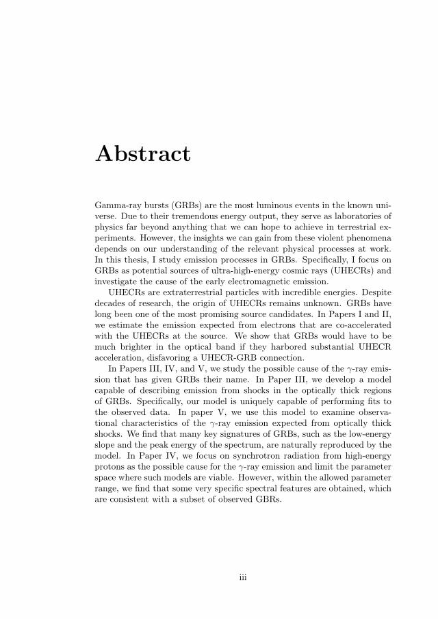
Abstract
Gamma-ray bursts (GRBs) are the most luminous events in the known uni-verse. Due to their tremendous energy output, they serve as laboratories ofphysics far beyond anything that we can hope to achieve in terrestrial ex-periments. However, the insights we can gain from these violent phenomenadepends on our understanding of the relevant physical processes at work.In this thesis, I study emission processes in GRBs. Specifically, I focus onGRBs as potential sources of ultra-high-energy cosmic rays (UHECRs) andinvestigate the cause of the early electromagnetic emission.
UHECRs are extraterrestrial particles with incredible energies. Despitedecades of research, the origin of UHECRs remains unknown. GRBs havelong been one of the most promising source candidates. In Papers I and II,we estimate the emission expected from electrons that are co-acceleratedwith the UHECRs at the source. We show that GRBs would have to bemuch brighter in the optical band if they harbored substantial UHECRacceleration, disfavoring a UHECR-GRB connection.
In Papers III, IV, and V, we study the possible cause of the γ-ray emis-sion that has given GRBs their name. In Paper III, we develop a modelcapable of describing emission from shocks in the optically thick regionsof GRBs. Specifically, our model is uniquely capable of performing fits tothe observed data. In paper V, we use this model to examine observa-tional characteristics of the γ-ray emission expected from optically thickshocks. We find that many key signatures of GRBs, such as the low-energyslope and the peak energy of the spectrum, are naturally reproduced by themodel. In Paper IV, we focus on synchrotron radiation from high-energyprotons as the possible cause for the γ-ray emission and limit the parameterspace where such models are viable. However, within the allowed parameterrange, we find that some very specific spectral features are obtained, whichare consistent with a subset of observed GBRs.
iii

iv
Sammanfattning
Gammablixtar (engelska “gamma-ray bursts”, GRBs) ar de mest ljusstarkafenomen vi kanner till i universum. Pa grund av deras otroliga energierger de oss mojligheten att studera fysik i miljoer vi aldrig skulle kunnaskapa i laboratorier pa jorden. Hur mycket kunskap vi kan fa om dessafenomen beror dock pa hur val vi forstar oss pade relevanta fysikaliska pro-cesserna. I denna avhandling studerar jag stralningsprocesser i GRBs. Merspecifikt, sa undersoker jag huruvida GRBs kan accelerera hogenergetiskkosmisk stralning (engelska “ultra-high energy cosmic rays”, UHECRs) ochursprunget for den elektromagnetiska stralningen.
Varifran UHECRs kommer ar fortfarande okant trots decennier av forskn-ing. GRBs har lange varit en av de mest lovande kallorna. I Artikel I ochII studerar vi stralningen fran elektroner som accelereras pa samma platssom UHECRs. Vi visar att om GRB var effektiva acceleratorer av UHE-CRs sa skulle de nodvndigtvis behova vara mycket mer ljusstarka i optiskavaglangder. Detta talar emot att GRBs som de primara kallorna for UHE-CRs.
I Artikel III, IV och V studerar vi uppkomsten till γ-stralningen somgett GRBs sitt namn. I Artikel III utvecklar vi en modell som kan simulerashocker i de optiskt tjocka delarna av en GRB. Modellen ar den forsta isitt slag som kan anvandas for anpassning av data. I Artikel V anvander videnna model for att analysera vilka typer av observationella signaturer mankan forvanta sig av shocker i de optiskt tjocka delarna. Vi finner att mangaegenskaper hos GRBs naturligt reproduceras av modellen, t.ex. lutningvid laga energier och hogsta energin i spektrat. I Artikel IV studerar vihogenergetiska protoner som mojligt orsak till γ-stralningen och begransarden mojliga parameterrymden for liknande modeller. Dar modellen fungerarvisar vi att man kan forvanta sig vissa saregna karaktarsdrag i spektrat, somfaktiskt liknar beteendet hos en del GRBs.
v

vi
List of Publications
Publications Included in the Thesis
Paper I
The Limited Contribution of Low- and High-luminosity Gamma-Ray Burststo Ultra-high-energy Cosmic Rays.Samuelsson, Filip, Begue, Damien, Ryde, Felix, and Pe’er, Asaf.The Astrophysical Journal, 876:93 (2019).DOI: 10.3847/1538-4357/ab153c.
Author’s contribution: The idea behind the paper was thought of byDamien Begue, Felix Ryde, and myself. I wrote all of the text in the article.I generated all figures and made all calculations, which were double checkedby Damien Begue. Throughout the development of the paper, all co-authorswere involved in continuous discussion. All co-authors helped proof-read themanuscript several times, which heavily influenced and improved the work.
Paper II
Constraining Low-luminosity Gamma-Ray Bursts as Ultra-high-energy Cos-mic Ray Sources Using GRB 060218 as a Proxy.Samuelsson, Filip, Begue, Damien, Ryde, Felix, Pe’er, Asaf, and Kohta,Murase.The Astrophysical Journal, 902:148 (2020).DOI: 10.3847/1538-4357/abb60c.
Author’s contribution: The paper is a continuation of Paper I and aconsequence of the discussions with Kohta Murase that followed the publi-cation of Paper I. I wrote all of the text and generated all of the figures. Thecode used in the afterglow scenario is written by Asaf Pe’er. The continuousdiscussion between all co-authors helped shape and re-shape the paper. Allco-authors helped proof-read the manuscript several times.
vii
viii List of Publications
Paper III
An efficient method for fitting radiation-mediated shocks to gamma-ray burstdata: The Kompaneets RMS approximation.Samuelsson, Filip, Lundman, Christoffer, and Ryde, Felix.The Astrophysical Journal, 902:148 (2020).DOI: 10.3847/1538-4357/ac332a.
Author’s contribution: The idea for the paper came from ChristofferLundman, who realized that the evolution of the photon spectrum in aradiation-mediated shock could be approximated using the Kompaneetsequation. Christoffer Lundman, Felix Ryde, and I developed the Kom-paneets RMS approximation together. I led the work, generated all figures,and wrote the simulation code Komrad upon which all results are based.Christoffer Lundman and I wrote the text together.
Paper IV
Bethe-Heitler signature in proton synchrotron models for gamma-ray bursts.Begue, Damien, Samuelsson, Filip, and Pe’er, Asaf.Manuscript submitted to The Astrophysical Journal.arXiv identifier: 2112.07231.
Author’s contribution: The idea for the paper originally came fromDamien Begue, which was developed further through discussion with AsafPe’er and myself. I obtained the early results. Damien Begue did all cal-culations, which I then double checked. Damien Begue wrote most of themanuscript during continuous discussion with me. I contributed in polishingand proof-reading the manuscript multiple times.
Paper V
Observational characteristics of radiation-mediated shocks in photosphericgamma-ray burst emission.Samuelsson, Filip and Ryde, Felix.Draft version of manuscript included.
Author’s contribution: The idea for the paper came from Felix Ryde,Christoffer Lundman, and myself as a natural continuation of Paper III. I ledthe work, did all calculations, generated all figures, and wrote all text. Thefinal version of the manuscript has been heavily influenced by continuousdiscussion with Felix Ryde.
Contents
Abstract iii
Sammanfattning v
List of Publications vii
Contents ix
1 Introduction 1
1.1 Gamma-ray bursts . . . . . . . . . . . . . . . . . . . . . . . 1
1.2 Cosmic rays . . . . . . . . . . . . . . . . . . . . . . . . . . . 2
1.3 Shocks . . . . . . . . . . . . . . . . . . . . . . . . . . . . . . 4
1.4 Context . . . . . . . . . . . . . . . . . . . . . . . . . . . . . 4
1.5 Conventions . . . . . . . . . . . . . . . . . . . . . . . . . . . 5
2 Physical processes 9
2.1 Special relativity . . . . . . . . . . . . . . . . . . . . . . . . 9
2.2 Optical depth . . . . . . . . . . . . . . . . . . . . . . . . . . 13
2.3 Random walk . . . . . . . . . . . . . . . . . . . . . . . . . . 15
2.4 Synchrotron radiation . . . . . . . . . . . . . . . . . . . . . 16
2.4.1 Characteristic timescale . . . . . . . . . . . . . . . . 17
2.4.2 Characteristic frequency . . . . . . . . . . . . . . . . 18
2.4.3 Photon spectrum . . . . . . . . . . . . . . . . . . . . 18
2.5 Compton scattering . . . . . . . . . . . . . . . . . . . . . . 23
2.5.1 Energy gain per scattering . . . . . . . . . . . . . . . 24
2.5.2 The Kompaneets equation . . . . . . . . . . . . . . . 26
2.6 Photohadronic interactions . . . . . . . . . . . . . . . . . . 29
2.6.1 Bethe-Heitler pair production . . . . . . . . . . . . . 29
2.6.2 High-energy neutrino production . . . . . . . . . . . 30
ix
x Contents
3 GRB physics 31
3.1 Observations . . . . . . . . . . . . . . . . . . . . . . . . . . 31
3.1.1 Light curves . . . . . . . . . . . . . . . . . . . . . . . 31
3.1.2 Short versus long GRBs . . . . . . . . . . . . . . . . 32
3.1.3 Spectra . . . . . . . . . . . . . . . . . . . . . . . . . 34
3.1.4 Low-luminosity GRBs . . . . . . . . . . . . . . . . . 35
3.1.5 Afterglow . . . . . . . . . . . . . . . . . . . . . . . . 37
3.2 Fireball model . . . . . . . . . . . . . . . . . . . . . . . . . 39
3.2.1 General evolution . . . . . . . . . . . . . . . . . . . . 39
3.2.2 Temperature and photon number . . . . . . . . . . . 40
3.2.3 Internal collisions . . . . . . . . . . . . . . . . . . . . 42
3.3 Photospheric emission . . . . . . . . . . . . . . . . . . . . . 44
3.3.1 Blackbody radiation . . . . . . . . . . . . . . . . . . 45
3.3.2 Broadening effects: non-dissipative photospheric spec-trum . . . . . . . . . . . . . . . . . . . . . . . . . . . 45
3.3.3 Subphotospheric dissipation . . . . . . . . . . . . . . 48
3.4 Prompt synchrotron emission . . . . . . . . . . . . . . . . . 48
3.4.1 Optically thin shocks . . . . . . . . . . . . . . . . . . 50
3.4.2 Low-energy slope . . . . . . . . . . . . . . . . . . . . 50
3.4.3 Proton synchrotron emission . . . . . . . . . . . . . 51
4 Shock physics 55
4.1 Shock properties . . . . . . . . . . . . . . . . . . . . . . . . 55
4.1.1 Nomenclature and conventions . . . . . . . . . . . . 55
4.1.2 Entropy increase . . . . . . . . . . . . . . . . . . . . 56
4.1.3 Shock jump conditions . . . . . . . . . . . . . . . . . 57
4.1.4 Speed after relativistic collision . . . . . . . . . . . . 59
4.2 Diffusive shock acceleration . . . . . . . . . . . . . . . . . . 60
4.3 Radiation mediated shocks . . . . . . . . . . . . . . . . . . 62
4.3.1 Radiation dominance and interaction scales . . . . . 63
4.3.2 Jump conditions in RMS with vanishing pair content 66
5 UHECR physics 69
5.1 Observations . . . . . . . . . . . . . . . . . . . . . . . . . . 69
5.1.1 Detection . . . . . . . . . . . . . . . . . . . . . . . . 69
5.1.2 Spectrum . . . . . . . . . . . . . . . . . . . . . . . . 70
5.1.3 Composition . . . . . . . . . . . . . . . . . . . . . . 71
5.2 Hillas criterion . . . . . . . . . . . . . . . . . . . . . . . . . 72
5.3 Magnetic field strength . . . . . . . . . . . . . . . . . . . . . 73
5.4 Energy budget . . . . . . . . . . . . . . . . . . . . . . . . . 75
Contents xi
6 Summary of attached papers 796.1 Paper I . . . . . . . . . . . . . . . . . . . . . . . . . . . . . 796.2 Paper II . . . . . . . . . . . . . . . . . . . . . . . . . . . . . 806.3 Paper III . . . . . . . . . . . . . . . . . . . . . . . . . . . . 816.4 Paper IV . . . . . . . . . . . . . . . . . . . . . . . . . . . . 826.5 Paper V . . . . . . . . . . . . . . . . . . . . . . . . . . . . . 83
Acknowledgments 85
Bibliography 87

xii
Chapter 1
Introduction
1.1 Gamma-ray bursts
Gamma-ray bursts (GRBs) are violent cosmic phenomena that release anenormous amount of energy on a timescale of seconds. They can be chat-egorized into two different classes. Long GRBs have observed durations of& 2 s and occur in connection with supernovae (SNe). Short GRBs haveobserved timescales . 2 s and happen during the merger of two neutronstar, or possibly a neutron star and a black hole. Observationally, bothclasses are quite similar, in that they manifest themselves as short brightflashes of gamma-ray radiation; the most energetic part of the electromag-netic spectrum. During its few active seconds, a GRB shines brighter thanall the other stars in its host galaxy combined.
Luckily for life on Earth, ionizing gamma-rays cannot penetrate Earth’satmosphere. On the downside, this means that the high-energy emissionfrom GRBs cannot be directly observed from Earth’s surface. Therefore,it was not until the advent of space born gamma-ray satellites that theseobjects were discovered. The first observed GRB was detected by the Velamission launched by the United States in 1967. The purpose of the Velamission was to make sure the Soviet Union adhered to the recently signedPartial Test Ban Treaty, which dictated that no nation was allowed to det-onate nuclear weapons above ground. The Vela satellites did see flashesof gamma-ray emission but it was not coming from the direction of Earth(Schilling, 2002). When the data was declassified six years later, it promptlyresulted in hundreds of theoretical models trying to explain the discovery.
Most of the new theories assumed the emission came from within ourown galaxy. The main motivation for this was the enormous energy requiredif the sources were not local to the Milky Way. A GRB actually emits
1
2 Chapter 1. Introduction
the same amount of energy during its ∼ 10 second emission period as theSun will radiate during its entire ten billion year lifetime (∼ 1051 erg).Thus, it is hardly surprising that early models focused on nearby sources.However, with the launch of the BATSE instrument in 1991, one foundthat GRBs were evenly spaced across the sky. This suggested that theydid not originate in the Milky Way, as one would then expect a higherconcentration of events in the galactic disc. This, therefore, hinted towardstheir extragalactic origin.
Today it is known that GRBs are indeed extragalactic and can be seenalmost across the entire observable Universe. The reason for there high ap-parent brightness is the same as why they are visible to such great distances:the emission is highly collimated into two narrow jets. The jets make themsimilar to a cosmic laser, increasing their visibility distance. Presently weknow a lot more about GRBs than we did fifty years ago. However, dueto their very short duration and wide variety of appearances, many of theirproperties still remain highly debated.
1.2 Cosmic rays
Cosmic rays (CRs) are badly named, since they are not rays at all. Theyare particles. However, this was unknown to physicists at the start of thelast century when one started to discover ionizing radiation from the atmo-sphere. In 1910, a German physicist by the name of Theodor Wulf climbedthe Eiffel tower with a electroscope that measured ionizing radiation. Sur-prisingly and against his own hypothesis, the ionizing radiation increasedwith height, which seemed to indicate that it was not coming from Earth(Wulf, 1910). In 1911, Nobel laureate Victor Hess built upon this discoveryby ascending in a ballon to an altitude of more than a kilometer. With anelectroscope of his own, he confirmed the findings of Wulf (Hess, 1912).
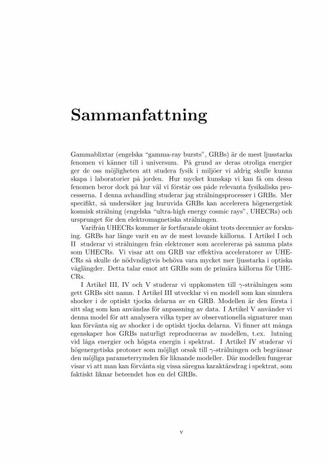
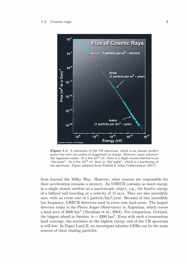
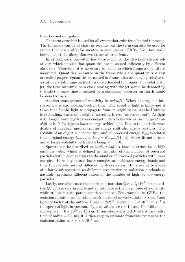
CRs are charged particles that are accelerated in various astrophysicalenvironments. They extend with an almost perfect power-law slope overan impressive ten orders of magnitude, from ∼ 1 GeV up to ∼ 102 EeV(Exa = 1018 being a prefix one gets to use much too rarely), see figure1.1. CRs are deflected in the galactic magnetic field due to their electriccharge. Thus, one cannot use their arrival direction to determine theirorigin. However, the sources of lower energy CRs are mostly known. Atthe lowest energy end, solar winds accelerate CRs up to a few GeV and inthe intermediate range, galactic supernova remnants are believed to be theprimary sources.
Ultra-high-energy cosmic rays (UHECRs) are CRs at energies above afew 1018 eV. They are so energetic that the galactic magnetic field is notstrong enough to contain them. Thus, observed UHECRs are most likely
1.2. Cosmic rays 3
Figure 1.1. A schematic of the CR spectrum, which is an almost perfectpower law over ten orders of magnitude in energy. However, some notewor-thy signature exists. At a few 1015 eV, there is a slight excess referred to as“the knee”. At a few 1018 eV there is “the ankle”, which is a hardening ofthe spectrum. Figure adopted from Pinfold & Atlas Collaboration (2017).
from beyond the Milky Way. However, what sources are responsible fortheir acceleration remains a mystery. An UHECR contains as much energyin a single atomic nucleus as a macroscopic object, e.g., the kinetic energyof a billiard ball traveling at a velocity of 15 m/s. They are also incrediblyrare, with an event rate of 1 particle/km2/year. Because of this incrediblylow frequency, UHECR detectors need to cover vast land areas. The largestdetector today is the Pierre Auger Observatory in Argentina, which coversa land area of 3000 km2 (Abraham et al., 2004). For comparison, Gotland,the biggest island in Sweden, is ∼ 3200 km2. Even with such a tremendousland coverage, the statistics at the highest energy end of the CR spectrumis still low. In Paper I and II, we investigate whether GRBs can be the mainsources of these eluding particles.
4 Chapter 1. Introduction
1.3 Shocks
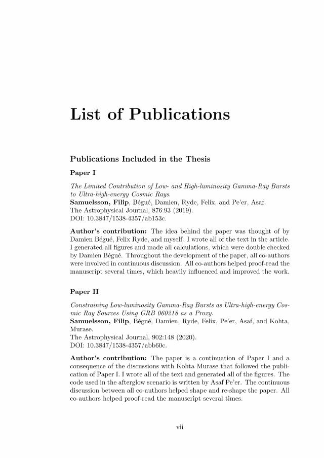
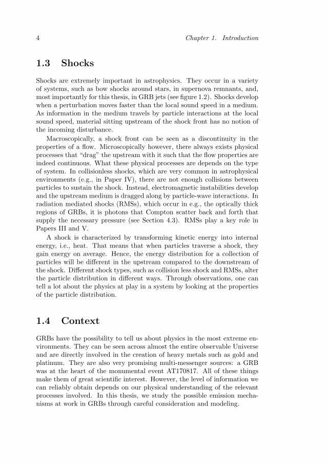
Shocks are extremely important in astrophysics. They occur in a varietyof systems, such as bow shocks around stars, in supernova remnants, and,most importantly for this thesis, in GRB jets (see figure 1.2). Shocks developwhen a perturbation moves faster than the local sound speed in a medium.As information in the medium travels by particle interactions at the localsound speed, material sitting upstream of the shock front has no notion ofthe incoming disturbance.
Macroscopically, a shock front can be seen as a discontinuity in theproperties of a flow. Microscopically however, there always exists physicalprocesses that “drag” the upstream with it such that the flow properties areindeed continuous. What these physical processes are depends on the typeof system. In collisionless shocks, which are very common in astrophysicalenvironments (e.g., in Paper IV), there are not enough collisions betweenparticles to sustain the shock. Instead, electromagnetic instabilities developand the upstream medium is dragged along by particle-wave interactions. Inradiation mediated shocks (RMSs), which occur in e.g., the optically thickregions of GRBs, it is photons that Compton scatter back and forth thatsupply the necessary pressure (see Section 4.3). RMSs play a key role inPapers III and V.
A shock is characterized by transforming kinetic energy into internalenergy, i.e., heat. That means that when particles traverse a shock, theygain energy on average. Hence, the energy distribution for a collection ofparticles will be different in the upstream compared to the downstream ofthe shock. Different shock types, such as collision less shock and RMSs, alterthe particle distribution in different ways. Through observations, one cantell a lot about the physics at play in a system by looking at the propertiesof the particle distribution.
1.4 Context
GRBs have the possibility to tell us about physics in the most extreme en-vironments. They can be seen across almost the entire observable Universeand are directly involved in the creation of heavy metals such as gold andplatinum. They are also very promising multi-messenger sources: a GRBwas at the heart of the monumental event AT170817. All of these thingsmake them of great scientific interest. However, the level of information wecan reliably obtain depends on our physical understanding of the relevantprocesses involved. In this thesis, we study the possible emission mecha-nisms at work in GRBs through careful consideration and modeling.
1.5. Conventions 5
Figure 1.2. Examples of shocks found in different astrophysical environ-ments. The left image shows the Crab nebula, which is a galactic supernovaremnant. The middle is a bow shock around a star in the Orion nebula.The right is a snapshot of a GRB jet simulation. Figures adopted fromNASA, ESA, J. Hester and A. Loll (2004) (left), NASA Science Official(1995) (middle), and Gottlieb et al. (2019) (right).
Papers I and II focus on the possible connection between UHECRs andGRBs. UHECRs require immense magnetic fields to be accelerated. Giventhat UHECRs are accelerated, one can calculate the emission from the elec-trons present at the source. We characterize the radiation from the electronsand compare it with observations of high- and low-luminosity GRBs. Themethods used in these papers are general and are useful tools that can beapplied to other UHECR candidates. In Paper III, we develop an approx-imation capable of quickly, yet accurately, capture the behavior of shocksthat occur in the optically dense parts of a GRB jet for the first time. InPaper IV, we study proton synchrotron emission as the cause of the high-energy gamma-ray emission in GRBs. Specifically, we find a smoking gunobservational signature from secondary Bethe-Heitler pairs created at thesource. In Paper V, we use the model developed in Paper III to characterizeobservational characteristics of optically dense shocks in GRB jets. We findthat such shocks can explain many of the observed GRB properties.
Some sections in this thesis are based upon similar ones from my licen-tiate thesis (Samuelsson, 2020). This is relevant for the sections that treatconcepts related to Papers I and II, as these were the papers included inmy licentiate thesis. These sections are: 1.5, 2.1, 2.2, 2.4, 3.1, 5.2, 5.3, 5.4,6.1, and 6.2.
1.5 Conventions
Here, I mention some of the important physical quantities and nomenclatureused in this thesis. Hopefully, this may help the unexperienced reader in
6 Chapter 1. Introduction
some of her inevitable confusion when reading. The list presented herebuilds upon a similar list from my licentiate thesis.
This thesis and the astronomy community in general work within thecentimeter-gram-second (CGS) unit system, as compared to the standardSI-system. Energies of individual particles are most often given in electronvolts (eV). The electron volt is defined as the kinetic energy an electroninitially at rest gains when accelerated in an electric potential of 1 volt.Some typical energies are the energy of optical photons ∼ 1 eV, typicalphoton energy in a GRB ∼ 300 keV, the proton rest mass energy ∼ 1 GeV,and UHECRs > 1 EeV (1018 eV). Collective energies of events are givenin erg, where 1 erg = 10−7 joule. The total energy output of a GRB is1051–1054 erg.
The luminosity [erg s−1] of an event is its energy output per unit time.It is common to define different types of luminosities, such as the radiationluminosity being the energy output specifically in radiation per unit time.Flux [erg s−1 cm−2] is energy per unit time per unit area. If the distanced to the object is known, the observed flux F is related to the intrinsic(original) luminosity of an object L by F = L/4πd2. Here, I assumedthat the luminosity was evenly spread in all directions, that the extinctionthat occur during the propagation to Earth was negligible, and ignored thereddening of radiation that occurs when light moves through our expandingUniverse. The fluence [erg cm−2] of an event is the flux integrated over theevent duration. For radiation, the spectral flux density [erg s−1 cm−2 Hz−1]is the flux per unit frequency. The spectral flux density, denoted by Fν , canalso sometimes be called the specific flux, spectral flux, or simply flux. As thefrequency of a photon is directly proportional to its energy, the spectral fluxdensity can also be given by Fε [erg s−1 cm−2 eV−1]. In radio astronomy,it is common to use to unit Jansky (Jy), defined as 1 Jy= 10−23 erg s−1
cm−2 Hz−1.
Detected signals contain information about the arrival time of particlesand their energies. A figure that plots particle number (or flux) versusarrival time is called a light curve. A light curve can be shown for particleswithin a specific energy range. A spectrum plots differential particle number(or differential flux) versus energy. A spectrum requires a specified timeinterval to indicate what particles are included. A time integrated spectrumincludes all particles observed from an event while a time resolved spectrumshows only particles within a specified time range.
The prefix circum is often used to mean “around”. For instance, cir-cumstellar material means the material surrounding a star. Similarly, interis used to describe “in between”. The intergalactic medium is the materialbetween galaxies. The prefix extra is used to mean “beyond”. Light thatis extraterrestrial is not from Earth and particles that are extragalactic are
1.5. Conventions 7
from beyond our galaxy.The term transient is used for all events that exist for a limited timescale.
The timescale can be as short as seconds but the term can also be used forevents that are visible for months or even years. GRBs, SNe, fast radiobursts, and tidal disruption events are all transients.
In astrophysics, one often has to account for the effects of special rel-ativity, which implies that quantities are measured differently by differentobservers. Therefore, it is necessary to define in which frame a quantity ismeasured. Quantities measured in the frame where the quantity is at restare called proper. Quantities measured in frames that are moving relative toa stationary lab frame on Earth is often denoted by primes. In a relativisticjet, the time measured on a clock moving with the jet would be denoted byt′ while the same time measured by a stationary observer on Earth wouldbe denoted by t.
Another consequence of relativity is redshift. When looking out intospace, one is also looking back in time. The speed of light is finite and ittakes time for the light to propagate from its origin to us. As the Universeis expanding, waves of a original wavelength gets “stretched out”. As lightwith longer wavelength is less energetic, this is known as cosmological red-shift as it shifts light to lower-energy, redder light. Due to the particle-waveduality of quantum mechanics, this energy shift also affects particles. Theredshift of an object is denoted by z and an observed energy Eobs is relatedto an original energy Esource as Eobs = Esource/(1+z). More distant objectsare at larger redshifts with Earth being at z = 0.
Spectra can be described as hard or soft. A hard spectrum has a highhardness ratio, which is defined as the ratio of the number of observedparticles with higher energies to the number of observed particles with lowerenergies. Here, higher and lower energies are arbitrary energy bands andthus there exists several different hardness ratios. It is useful to speakof a hard/soft spectrum as different acceleration or radiation mechanismsnaturally produces different ratios of the number of high- to low-energyparticles.
Lastly, one often uses the shorthand notation QX ≡ Q/10X for quanti-ties Q. This is very useful to get an estimate of the magnitude of a quantitywhile still seeing its parameter dependence. For example, in GRBs, theemission radius r can be estimated from the observed variability time t andLorentz factor of the outflow Γ as r = 2ctΓ2, where c = 3× 1010 cm s−1 isthe speed of light in vacuum. Typical values are t ∼ 1 s and Γ ∼ 100 so onecan write r = 6 × 10¹⁴ t0 Γ2
2 cm. If one observes a GRB with a variabilitytime of only t = 50 ms, it is then easy to estimate from this expression theemission radius as r = 3× 1013 cm.

8
Chapter 2
Physical processes
In this chapter, I outline some of the basic physical concepts needed tounderstand subsequent chapters and the attached papers. It is not feasibleto give a complete account for each of the different subjects, for that I referthe reader to designated text books.
2.1 Special relativity
Object moving with velocities close to the speed of light are called rela-tivistic, as one must account for the effects of special relativity. Relativisticeffects appear everywhere in this thesis, from GRB jets, to synchrotron elec-trons, to UHECRs. For a good introduction to the field of special relativity,I refer to chapter 2 of Harris (2008). Here, I give a short account of somerelevant effects.
Lorentz factor. The Lorentz factor γ (or Γ) is a central concept of rela-tivity. An objects Lorentz factor is solely a function of its velocity v and isdefined as
γ =1√
1− (v/c)2(2.1)
where c is the speed of light in vacuum. As nothing can move faster than c,one can see from the equation above that γ ≥ 1 is always satisfied. Whenγ grows larger than unity, traditional Newtonian mechanics breaks down.Newtonian mechanics is a great approximation for everyday objects wherethe effects of relativity are unnoticeable. In astrophysics however, this is nolonger the case. In GRB physics, one often refers to the Lorentz factor ofthe bulk outflow by capital Γ and the Lorentz factors of particles (electrons,
9
10 Chapter 2. Physical processes
protons, and nuclei) by lower case γ′. Here, the prime denotes that theLorentz factor is most often evaluated in the outflow frame, i.e., the parti-cles are relativistic even as seen from an observer traveling with the outflow.
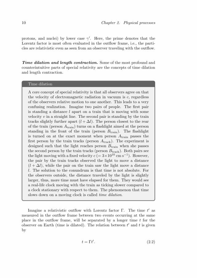
Time dilation and length contraction. Some of the most profound andcounterintuitive parts of special relativity are the concepts of time dilationand length contraction.
Time dilation
A core concept of special relativity is that all observers agree on thatthe velocity of electromagnetic radiation in vacuum is c, regardlessof the observers relative motion to one another. This leads to a veryconfusing realization. Imagine two pairs of people. The first pairis standing a distance l apart on a train that is moving with somevelocity v in a straight line. The second pair is standing by the traintracks slightly further apart (l+ ∆l). The person closest to the rearof the train (person Atrain) turns on a flashlight aimed at the personstanding in the front of the train (person Btrain). The flashlightis turned on at the exact moment when person Atrain passes thefirst person by the train tracks (person Atrack). The experiment isdesigned such that the light reaches person Btrain when she passesthe second person by the train tracks (person Btrack). Both pairs seethe light moving with a fixed velocity c (= 3×1010 cm s−1). However,the pair by the train tracks observed the light to move a distance(l + ∆l), while the pair on the train saw the light move a distancel. The solution to the conundrum is that time is not absolute. Forthe observers outside, the distance traveled by the light is slightlylarger, thus, more time must have elapsed for them. They would seea real-life clock moving with the train as ticking slower compared toa clock stationary with respect to them. The phenomenon that timeslows down on a moving clock is called time dilation.
Imagine a relativistic outflow with Lorentz factor Γ. The time t′ asmeasured in the outflow frame between two events occurring at the sameplace in the outflow frame, will be separated by a longer time t for theobserver on Earth (time is dilated). The relation between t′ and t is givenby
t = Γt′. (2.2)
2.1. Special relativity 11
The length l′ of an object at rest in one frame is contracted for an observerthat is moving relative to this frame by
l =l′
Γ. (2.3)
Time dilation and length contraction are unavoidable consequences of thepostulates of special relativity.
Beaming. Driving a car while the rain is pouring down, it is possible toget the sensation that the rain drops are hitting the windshield almost ver-tically, although the rain is falling straight towards the ground. A relatedeffect happens with moving emitters of light. Radiation emitted isotropi-cally by a source moving with Lorentz factor γ compared to an observer onEarth is beamed in the direction the source is moving. The beaming is suchthat half of the radiation is emitted into a cone with opening angle θ ∼ 1/γ.Consequently, objects moving away from us with γ 1 can be virtuallyundetectable, as most of the light is beamed in the opposite direction. GRBjets have outflow Lorentz factors Γ 1. Thus, a distant GRB can only bedetected if one of the jets is pointing towards Earth.
Blueshift, redshift, and Doppler factor. Radiation emitted with afrequency νsource by a moving source will be observed as having a differentfrequency νobs. The two frequencies are related as
νobs = δνsource = γνsource
(1 +
v
ccos θ
), (2.4)
where v is the velocity of the emitter and θ is the angle between the velocityvector of the source to the line of sight. The factor δ ≡ γ
(1 + v
c cos θ)
iscalled the relativistic Doppler factor. The term in the parenthesis is anal-ogous to the traditional Doppler shift for sound waves that one can hearwhen an ambulance drives by. The γ-factor is a relativistic effect that ac-counts for time dilation. An observed photon is blueshifted if the observedfrequency is higher than the emitted frequency (source moving towards theobserver) and redshifted otherwise. The names stem from the fact that bluevisible light is more energetic than red light. However, the terms blue- andredshift are used for all electromagnetic bands, not just in the optical.
Velocity transformation. Imagine some object U traveling with velocityu and some other object V traveling with velocity v with respect to the lab
12 Chapter 2. Physical processes
frame. If one wants to find the velocity of object U as seen by an observerin V’s frame, it is given by
u′ =u− v
1− uv/c2⇐⇒ βu′ =
βu − βv1− βuβv
, (2.5)
where βi is the velocity of object i divided by c, e.g., βu = u/c. It is ofteruseful with an expression for the Lorentz factor of object U in V’s frame interms of the the Lorentz factors γu and γv as seen in the lab frame. Fromequation (2.1) we have
γu′ =1√
1− β2u′
=⇒ (2.6)
Using the right hand part of equation (2.5), one gets
β2u′ =
(βu − βv1− βuβv
)2
=β2u + β2
v − 2βuβv(1− βuβv)2
=
(1− 1
γ2u
)+(
1− 1γ2v
)− 2βuβv
(1− βuβv)2,
(2.7)where I used β2
i = 1 − 1/γ2i . Inserting this back into equation (2.6), one
gets
γu′ =1√
1− β2u′
=1− βuβv√
−1 + β2uβ
2v + 1/γ2
u + 1/γ2v
, (2.8)
where we multiplied top and bottom with (1 − βuβv) and expanded (1 −βuβv)
2 within the root. Now,
β2uβ
2v =
(1− 1
γ2u
)(1− 1
γ2v
)= 1− 1
γ2v
− 1
γ2u
+1
γ2vγ
2u
, (2.9)
so the whole thing simplifies to
γu′ =1− βuβv√
1/γ2uγ
2v
= (1− βuβv)γvγu, (2.10)
Thus, the relation between the three Lorentz factors is
γu′ = (1− βuβv)γuγv ≈γv2γu
+γu2γv− 1
4γuγv, (2.11)
where the first equality is exact and the second is valid for large γu and γv.The relation for the relativistic four-velocity, given by γu′βu′ , is then
γu′βu′ = (βu − βv)γuγv ≈γu2γv− γv
2γu, (2.12)
where the approximation is again valid for large γu and γv.
2.2. Optical depth 13
Useful Taylor expansions. In a GRB jet, the bulk of the outflow travelsat extremely relativistic speeds. Common Lorentz factors are in the orderof Γ ≈ 300, which corresponds to a velocity of 99.9994% the speed of light.In these highly relativistic regimes, one can make many simplifying Taylorexpansions. I list some of them here
β ∼ 1− 1
2Γ2, (2.13)
which gives
Γβ ∼ Γ− 1
2Γ. (2.14)
From equation (2.13), one also gets
1− β ∼ 1
2Γ2, (2.15)
Difference between two velocities is given by
β2 − β1 ∼1
2Γ21
− 1
2Γ22
∼ 1
2Γ21
if Γ1 Γ2. (2.16)
2.2 Optical depth
Of central importance in this thesis is the concept of optical depth. Theoptical depth, τ , is a measure of how likely a photon is to interact (scatteror be absorbed) while moving some distance between r0 and r. It is definedas
τ(r) =
∫ r
r0
n(r)σ(r) dr, (2.17)
where r is a parameter of integration and n is the particle density with whichthe photon can interact. The density can vary along r. The parameter σ iscalled the cross section.
14 Chapter 2. Physical processes
Cross section
Imagine a slab of width dx [cm]. Inside the slab, there are particlesdistributed with a number density n [cm−3]. What is the probabilityP that a photon traveling towards the slab interacts within the slab?Obviously, it should be a function of the particle density n. It isalso a function of the width dx: the wider the slab, the higher theprobability of interaction. Lastly, it is a function of the cross sectionσ [cm2] such that P = σndx. The intuitive way to think about thecross section is the influential area surrounding each of the particlesin the slab. If the photon passes within the influential area, it isclose enough to the particle such that it interacts.
In equation (2.17), the interaction process is not specified. It is possibleto look at the optical depth of a specific process by inserting the cross sectionfor that particular interaction (see e.g., Rees & Meszaros, 2005). However,it is commonly interesting to look at the overall interaction probability,in which case the cross section becomes a sum of all possible interactioncross sections. A medium is said to be optically thick if the optical depthintegrated over the medium size is larger than unity: τ > 1. Otherwise, themedium is optically thin. The photospheric radius of a GRB (see Section3.3) is defined as the radius from which the optical depth for a photontrapped in its fluid element to escape to infinity drops below one. Belowthe photospheric radius, photons are trapped within the outflow. Above thephotosphere, the photons can stream freely and reach the observer withoutfurther interaction. The photospheric radius is an approximation. In reality,photons experience their last scattering over a wide range of radii (Pe’er,2008; Lundman et al., 2013).
The mean free path [cm] of a photon is the length that it travels onaverage between interactions. It is often denoted by λ (or l) and is givenby λ = 1/nσ. If the density and cross section are constant across a slab ofwidth L, we see from equation (2.17) that
τ = nσL =L
λ, (2.18)
that is, the optical depth across a slab can be approximated as the width ofthe slab divided by the mean free path. In section 2.3, we see that the opticaldepth is, perhaps not surprisingly, connected to the number of scatteringson average a particle undergoes before escaping a system.
2.3. Random walk 15
2.3 Random walk
A key concept in particle scattering and diffusion theory is the concept ofrandom walk. Image a particle that is embedded in an isotropic pool ofparticles. It travels some distance before it scatters, after which it travelsin a random new direction until it scatters again. How far the particle hasmoved after N scatterings can be answered probabilistically (e.g., Rybicki& Lightman, 1979).
Let us call the total displacement R, where the bold font signifies thatit is a vector. The total displacement is the sum of all vector distancestraveled in between scatterings. If we denote the vector pointing from theorigin to the place of first scatting by r1, the vector pointing from the firstinteraction point to the place of the second scattering by r2, and so forth,we obtain
R = r1 + r2 + r3 + ...rN . (2.19)
We want to find the average displacement for a particle after N scatter-ings. However, averaging over equation (2.19) yields zero, since particlescan travel in all directions and R is a vector. To obtain the displacementl∗, we square both sides and then average, which gives
l2∗ =⟨R2⟩
=⟨r2
1
⟩+⟨r2
2
⟩+⟨r2
3
⟩+ ...+
⟨r2N
⟩+ 〈r1 · r2〉+ 〈r1 · r3〉+ ...
(2.20)
If we denote the mean free path by λ, then all N terms involving a squareof a displacement each average to
⟨r2i
⟩= λ2. The cross terms all average to
zero, as the dot product involves the cosine between the scattering vectorsas ri · rj = rirj cos(θ), and the average 〈cos(θ)〉 = 0, when all angles areequally likely. Thus, one gets that the average displacement in a randomwalk equals
l∗ =√Nλ. (2.21)
Say we have a medium of characteristic length L. If we set the total dis-placement equal to the characteristic length of the medium, l∗ = L, we getan estimate of the number of scatterings a particle undergoes before escap-ing the medium. Furthermore, if the density is constant across the medium,we found in section 2.2 that τ = L/λ. Using equation (2.21), one seesthat the characteristic number of scattering required to escape the systemis N ∼ τ2.
The above derivation is valid when the scattering is isotropic, i.e., whena particle is equally likely to scatter in any given direction. However, foran observer looking at a highly relativistic outflow with Lorentz factor Γ,a scattering that was isotropic in the rest frame of the outflow will be
16 Chapter 2. Physical processes
highly beamed into a cone with opening angle 1/Γ in the observers frame.Therefore, equation (2.20) becomes
l2? =⟨R2⟩
=⟨r2
1
⟩+⟨r2
2
⟩+⟨r2
3
⟩+ ...+
⟨r2N
⟩+ 〈r1 · r2〉+ 〈r1 · r3〉+ ... ≈ Nλ2 + (N − 1)Nλ2 = N2λ2,
(2.22)
where the additional term (N − 1)Nλ2 comes from the fact that particlesmostly travel in the same direction after a scattering as before, and hence〈ri · rj〉 = λ2 in this case. The number of scatterings to escape a mediumof size L is the relativistic case is thus N ∼ τ .
2.4 Synchrotron radiation
Electric charges in magnetic fields gyrate around the magnetic field linesaccording to Maxwell’s equations. If the charge had some initial velocityparallel to the magnetic field line, this velocity is unaltered. Thus, thecharged particles traces out a helical path following the magnetic field line.The gyration means that the particle experiences continuous accelerationand it therefore emits radiation. The frequency of the radiation producedthis way is proportional to the gyration period of the charged particle. Thistype of radiation is called cyclotron radiation. If the particle is relativistic,the emitted radiation is beamed and can only be seen in short, intermittentpulses when the particle is traveling towards the observer. The relativisticcase is called synchrotron radiation and is much more important in astro-physical environments. As the observed frequency is inversely proportionalto the pulse width according to Fourier analysis, the observed synchrotronfrequency is much higher than in the cyclotron case.
Synchrotron emission is important for the work in this thesis. The ac-celeration of UHECRs requires strong magnetic fields, which imply intensesynchrotron emission from the electrons that are also also accelerated atthe source. In Papers I and II, we calculate the synchrotron emission fromthe co-accelerated electrons and compare the estimated radiation to GRBobservations. Synchrotron radiation is also a core concept in Paper IV. InPaper IV, where we study the synchrotron emission from secondary pairscreated in photohadronic interactions between energetic protons and ambi-ent photons.
To be consistent with the nomenclature in Papers I and II, I use primesto indicate quantities evaluated in the frame comoving with the outflow.Unprimed quantities are measure in the observer frame.
2.4. Synchrotron radiation 17
2.4.1 Characteristic timescale
The total synchrotron power P ′ averaged over pitch angle emitted by acharged particle with Lorentz factor γ′, mass m, and charge number Z in amagnetic field B′ is given by (e.g., Rybicki & Lightman, 1979)
P ′ =4
3σTZ
4(me
m
)2
cβ′2γ′2B′2
8π. (2.23)
In the equation above, σT is the electron Thomson cross section and β′
is the velocity of the charged particle in terms of speed of light c. Fromequation 2.23 it is evident that the power emitted is inversely proportionalto the mass of the emitter squared. Therefore, electrons radiate their surplusenergy much more quickly compared to heavier particles, such as protons.This is relevant in Paper IV, see also section 3.4.3.
The power is energy emitted per unit time. In the differential limit, wehave P ′ = −dE′/dt′, where E′ = γ′mc2 is particle energy, t′ is the time,and the minus sign appears because the particle is losing energy. Insertingthis into equation (2.23), assuming the particle is highly relativistic β′ ∼ 1,and separating variables one gets
− dE′
E′2=
4
3σTZ
4(me
m
)2 c
(mc2)2
B′2
8πdt′, (2.24)
where I divided both sides by (γ′mc2)2. Integrating both sides and assumingthe magnetic field stays constant under the time scale considered implies
−∫ E′
final
E′initial
dE′
E′2=
1
E′final
− 1
E′initial
=4
3σTZ
4
(m
me
)2c
(mc2)2
B′2
8π(t′final − t′initial).
(2.25)
The time it takes the particle to lose half of its energy due to synchrotronradiation is thus
t′sync =6π
Z4σT
(me
m
)2 (mc2)2
c
1
E′B′2, (2.26)
where we have simply called E′initial for E′. The timescale t′sync is calledthe synchrotron energy loss timescale, or the characteristic synchrotrontimescale, for a particle of energy E′. It gives an estimate of how longtime it takes for a particle in a magnetic field with strength B′ to lose asignificant fraction of its energy to synchrotron radiation.
18 Chapter 2. Physical processes
2.4.2 Characteristic frequency
The angular frequency ω′ for an emitted photon by a non-relativistic particlewith massm can be obtained by equating the centripetal force to the Lorentzforce:
ma′centripetal =q
c(v′⊥ ×B′), (2.27)
where v′⊥ is the component of the velocity that is perpendicular to the mag-netic field B′. The magnitude of the centripetal acceleration is a′centripetal =
v′2/r′. Solving for the angular velocity ω′ ≡ v′/r′, one gets
ω′NR =qB′
mc. (2.28)
The frequency in equation (2.28) is called the cyclotron frequency, wherethe subscript NR stands for non-relativistic. The rotational frequency ν′ isequal to ν′ = ω′/2π. In the relativistic case, the emitted radiation is boostedby a factor of γ′2. The observed spectrum from an electron with Lorentzfactor γ′ will cover a range of energies but the characteristic synchrotronfrequency emitted is
ν′ =qB′
2πmcγ′2. (2.29)
The frequency given above is valid in the rest frame of the outflow. Toobtain the observed frequency, one has to account for the Doppler boost asgiven in equation (2.4).
2.4.3 Photon spectrum
From equation (2.29), it is evident that the emitted photon frequency de-pends on the Lorentz factors of the emitting particle. Hence, the observedphoton spectrum depends on the emitting particles energy distribution. InGRB applications, the shape of the spectrum is characterized by three spe-cific electron Lorentz factors: the injection Lorentz factor γ′m, the coolingLorentz factor γ′c, and the self-absorption Lorentz factor γ′SSA. Below I ex-plain the meaning of these three in turn.
Injection Lorentz factor. In GRBs and other astrophysical sources, oneoften assumes that the source distribution of particles is a power law. Thisis consistent with the theory of diffusive shock acceleration described inSection 4.2, as well as with particle-in-cell simulations (PIC, see e.g., Sironi& Spitkovsky, 2011; Crumley et al., 2019; Bohdan et al., 2020). Note thatnot all particles are accelerated into the power-law distribution, as discussed
2.4. Synchrotron radiation 19
in Paper II. If the total number of accelerated electrons is N , the power lawis written as
dN
dγ′= C ′γ′−p, γ′m < γ′ < γ′max, (2.30)
where C ′ is some proportionality constant and the power law extends fromthe minimum Lorentz factor γ′m to the maximum Lorentz factor γ′max. Thevariable p is called the spectral index. I will assume p > 2 in the followingderivation.
The minimum Lorentz factor γ′m is often called the injection Lorentzfactor. I can be estimated as follows (e.g., Meszaros, 2006). From equation(2.30) the number of accelerated particles in is obtained as
N =
∫ γ′max
γ′m
C ′γ′−pdγ′ =C ′
p− 1
(1
γ′p−1m
− 1
γ′p−1max
). (2.31)
The energy in the accelerated particles is
E′ = C ′mc2∫ γ′
max
γ′m
γ′−p+1dγ′ =C ′mc2
p− 2
(1
γ′p−2m
− 1
γ′p−2max
). (2.32)
Solving for C ′ from equation (2.31), we obtain
C ′ = N(p− 1)
(1
γ′p−1m
− 1
γ′p−1max
)−1
. (2.33)
Inserting into equation (2.32) yields
E′ = Nmc2γ′m(p− 1)
(p− 2)
1−(γ′m
γ′max
)p−2
1−(γ′m
γ′max
)p−1
(2.34)
Assuming that γ′max γ′m and p > 2, the large parenthesis in equation(2.34) is simply 1.
To proceed, one introduces the dimensionless quantity, ε, defined as thefraction of the internal energy behind the shock that is given to the acceler-ated particles. In a shock scenario, the shock dissipates some of the incomingkinetic energy and turn it into internal energy behind the shock E′int. Letsus assume the material in front of the shocks is stationary and consisting ofprotons and electrons. In the rest frame of the shock, the incoming particleshave a kinetic energy Np(Γ − 1)mpc
2 + Ne(Γ − 1)mc2 ≈ Np(Γ − 1)mpc2,
where Γ is the shock Lorentz factor and Np and Ne are the number of pro-tons and electrons respectively. This is roughly the energy that is converted
20 Chapter 2. Physical processes
into internal energy in the downstream. Out of this available energy, theaccelerated particles gets a fraction ε, i.e., E′ = εNp(Γ− 1)mpc
2.
The last thing is to introduce the fraction, ξa, as the number fractionof particles that are accelerated into the power law out of the total bulknumber, Ntot, such that N = ξaNtot. If the accelerated particle species isprotons, then Ntot = Np. If the accelerated particle species is electrons,then one commonly assumes charge neutrality such that Ntot = Ne = Np.Putting this together, one can solve for γ′m in equation 2.34 as
γ′m =p− 2
p− 1(Γ− 1)
mp
m
ε
ξa. (2.35)
The dependence of γ′m ∝ ε/ξa is quite intuitive. More energy given to theaccelerated particles (larger ε) results in higher γ′m and if fewer particlesshare the energy (smaller ξa) γ′m also increases.
Cooling Lorentz factor. The particles in the outflow mainly lose their en-ergy in two different ways, through their synchrotron emission and throughthe adiabatic expansion of the jet. The time scale for synchrotron energylosses has already been described in Section 2.4.1. The adiabatic losses comefrom the fact that as the jet moves outwards, it expands. The expansionimplies that the internal particles do work on the system. Macroscopically,it is a similar effect as when the temperature drops in a gas that expands inaccordance to the ideal gas law. Microscopically, the effect occurs becausein an expanding medium, particles are statistically more likely to scatterwith particles moving away from them than towards them, leading to anaverage energy loss.
For a reversible, adiabatic process, the temperature T ′ is related to thevolume V ′ as T ′ ∝ V ′1−γad , where γad is the adiabatic index (not to beconfused with a Lorentz factor). As the particles are highly relativistic,the adiabatic index is γad = 4/3. The comoving volume is proportional tothe radius cubed, which indicates that the comoving temperature drops asT ′ ∝ r−1. As the internal energy of the particles is proportional to thetemperature, it follows that a particle loses half of its energy due to theadiabatic expansion of the jet when r → 2r. The corresponding timescaleis
t′ad =r
cΓ, (2.36)
where the factor of Γ enter due to the length contraction of r in the outflowframe.
The cooling Lorentz factor of the electrons, γ′c, is defined as the Lorentzfactor where an electron would lose equal amount of energy to synchrotron
2.4. Synchrotron radiation 21
radiation as to the adiabatic expansion of the ejecta. It can be obtained byequating equations (2.26) and (2.36)
γ′c =6πmec
2
σT
Γ
rB′2. (2.37)
As t′ad is independent of energy while t′sync ∝ γ′−1, electrons with Lorentzfactor γ′ > γ′c cool mainly through synchrotron emission while electronswith Lorentz factor γ′ < γ′c cool mostly due to the adiabatic expansion.
Self-absorption Lorentz factor. The last important Lorentz factor is thesynchrotron self-absorption Lorentz factor, γ′SSA. The particles that emitsynchrotron radiation can themselves absorb the same radiation throughsynchrotron self-absorption. The absorption is preferential to low-energyemission leading to a sharp drop of flux towards low energies. Particles withLorentz factors less than γ′SSA effectively reabsorb photon, which increasestheir energy. The consequence is that very few particles have Lorentz factorsless than γ′SSA. The three Lorentz factors γ′m, γ′c, and γ′SSA have charac-teristic frequencies ν′m, ν′c, and ν′SSA, which are obtained by inserting thecorresponding Lorentz factor into equation (2.29).
Different emission regimes. Each particle that radiate synchrotronemission, emits over a range of frequencies. The overall shape of the photonspectrum emitted by a single particle is remarkably enough independent ofthat particles energy. For instance, the spectral flux density (flux per unitfrequency) in the low-energy tail of the spectrum is proportional to the fre-quency to power one third: Fν ∝ ν1/3 (Blumenthal & Gould, 1970; Rybicki& Lightman, 1979).
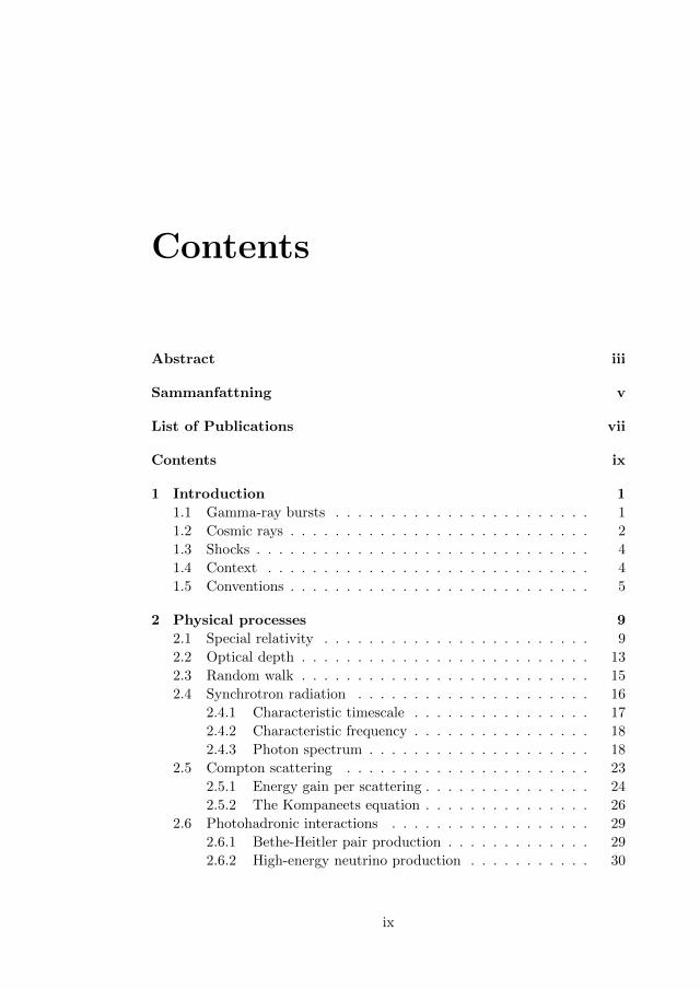
The observed spectrum is a superposition of photon spectrum emittedby all particles at the source. Hence, the distribution of the particles affectthe shape of the observed spectrum. If the particle distribution is isotropicand in a power law as defined in equation (2.30), then the spectral fluxvaries as Fν ∝ ν−(p−1)/2 (Blumenthal & Gould, 1970; Rybicki & Lightman,1979). However, this assumes that the power law does not change with time.Because of their synchrotron emission, the particles lose energy and cool,which alters the shape of the particle distribution. The general picture isthat the particles cool quickly due to synchrotron emission down to Lorentzfactor γ′c. Below γ′c, the particles are dominantly cooled by the adiabaticexpansion. However, this is a slow process (in comparison) and the particlescan be assumed to be static. Therefore, there exists two cases dependingon the position of γ′m relative to γ′c.
22 Chapter 2. Physical processes
10 3 10 2 10 1 100 101
[arb. units]10 3
10 2
10 1
100
F[a
rb. u
nits
]
FastMarginally fastSlow
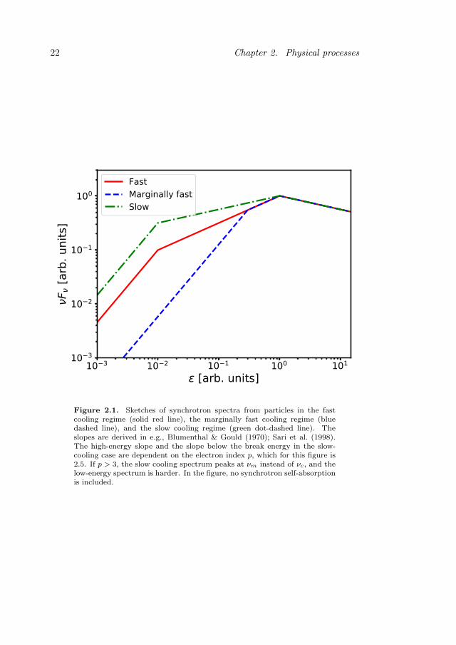
Figure 2.1. Sketches of synchrotron spectra from particles in the fastcooling regime (solid red line), the marginally fast cooling regime (bluedashed line), and the slow cooling regime (green dot-dashed line). Theslopes are derived in e.g., Blumenthal & Gould (1970); Sari et al. (1998).The high-energy slope and the slope below the break energy in the slow-cooling case are dependent on the electron index p, which for this figure is2.5. If p > 3, the slow cooling spectrum peaks at νm instead of νc, and thelow-energy spectrum is harder. In the figure, no synchrotron self-absorptionis included.
2.5. Compton scattering 23
Particles are in the so called the fast cooling regime if γ′m > γ′c. Inthis scenario, the particles cool down quickly to γ′c, where the cooling stops.Thus, below γ′c the spectrum is simply the combined low-energy tails, whichall satisfy Fν ∝ ν1/3. Between γ′m and γ′c, the cooling alters the shape ofthe spectrum such that Fν ∝ ν−1/2 (Sari et al., 1998). Above γ′m they arecontinuously injected with a slope −p, but they also cool. The power-lawinjection contributes a factor of −(p − 1)/2 and the cooling a factor −1/2to the particle index. The spectral slope is therefore Fν ∝ ν−p/2.
Particles are in the so called the slow cooling regime if γ′c > γ′m. Inthis case the particles injected below γ′c are assumed to be static due tothe inefficient cooling. Without efficient cooling the spectrum is given byFν ∝ ν−(p−1)/2, which is therefore appropriate between γ′m and γ′c. Aboveγ′c, we have to account for the cooling as well. Similarly to the fast coolingscenario, one gets Fν ∝ ν−p/2. Below γ′m the slope is the combined low-energy tail with Fν ∝ ν1/3. For both fast and slow cooling, the flux dropssteeply below the absorption frequency.
In synchrotron model fits of GRB prompt emission, one often finds thatparticles are in a marginally fast cooling regime, defined as γ′c . γ′m (Daigneet al., 2011; Ravasio et al., 2018, 2019; Oganesyan et al., 2019; Burgess et al.,2020). In a marginally fast cooling regime, it is possible to get sufficientenergy out in radiation while maintaining a quite hard low-energy slope.However, when the radiating particles are electrons, it is difficult to getγ′c comparable to γ′m without obtaining unexpected parameter estimations.This has led to the suggestion of proton synchrotron models (Ghiselliniet al., 2020; Florou et al., 2021; Mei et al., 2022). This is the motivationbehind the work in Paper IV. The three different regimes are shown in figure2.1.
2.5 Compton scattering
Electrons and photons interact with each other via Compton scattering.1 Ina scattering event, both the directions and the energies of the two scattererscan change. In the case where the incoming photon is more energetic thanthe incoming electron, the photon can impart some of its energy to theelectron. This interaction is called Compton scattering. Inverse Comptonscattering on the other hand is where the photon gains energy from theelectron. In inverse Compton scattering, the energy gain is proportional toLorentz factor of the electron squared (γ2), given that the photon energy
1Photons can scatter with other charged particles as well, such as protons. However,the cross section is inversely proportional to the mass squared, suppressing a scatteringbetween a photon and a proton by a factor (me/mp)2. In this section, I therefore focuson electrons.
24 Chapter 2. Physical processes
in the electron rest frame is smaller than the electron rest mass. As γ canbe very large, this process can results in very-high-energy photons. If thescattering between the electron and the photon is elastic, i.e., that no energyis transferred between the two, it is called Thomson scattering. Thomsonscattering is the low-energy limit of Compton scattering.
Photons
Due to the wave-particle duality of quantum mechanics, electromag-netic radiation can either be seen as a particle or as a wave. In thisthesis, we mostly work with high-energy electromagnetic radiation(X-rays and γ-rays). In that case, it is most convenient to thinkof light as particles. The particles are called photons and are thequanta of electromagnetic radiation. Although a photon is a parti-cle it still has an associated frequency ν. The frequency is relatedto the energy of the photon as ε = hν, where h is Planck’s con-stant. Scattering between electrons and photons can be visualizedas particles bouncing off of each other, sort of like when billiardballs collide. In the low-frequency limit (radio waves and infraredlight), the electromagnetic radiation is best described by a wave. Inthe interaction between a stationary electron and an incoming elec-tromagnetic wave, a scattering event is due to the charged particleoscillating in the incoming wave. The particle gains energy fromthe wave and then emits electromagnetic radiation due to its ownoscillation.
2.5.1 Energy gain per scattering
As photons carry momentum, the scattering of a photon with a particle isnot elastic. Using conservation of momentum and energy, one finds that inthe rest frame of the electron before the scattering, the final photon energyεf is related to the initial photon energy εi as
εf =εi
1 + εi(1− cosφ), (2.38)
where φ is the photon angle of deflection (see Figure 7.1 in Rybicki & Light-man, 1979) and the tildes indicate that the photon energies are evaluated inthe rest frame of the electron. The photon energies are given in units mec
2.When the photon energies are low compared to the electron rest mass, onecan Taylor expand the expression above to get
εf ≈ εi − ε2i (1− cosφ). (2.39)
2.5. Compton scattering 25
Commonly, the scattering particle is not at rest but moving at some velocity,e.g., from thermal motion. To see how the photon energy changes in a framewhere the scatterer is moving, one first needs to transform the photon energyinto the rest frame of the scatterer, see how the energy changes in thisframe using equation (2.38), and transform the photon energy back into theoriginal frame.
A heuristic argument to get the energy gain in this case is as follows.The energy of the photon in the electron rest frame is given by εi = δεi,where δ is the Doppler factor defined in equation (2.4) and εi is the initialphoton energy in the frame where the charge is moving. After the scattering,the photon should be transformed back as εf = δεf . The Doppler factorin this case is not the same as the previous one, as the photon directionhas changed. However, the magnitudes are on average similar, and we onlywant to make a heuristic argument. Thus,
εf ∼ δ2εi[1− δεi(1− cosφ)]. (2.40)
The Doppler factor is approximately the Lorentz factor of the moving scat-terer, γ. Furthermore, the cosine angle dependence will average to 0 whenlooking at an ensemble of isotropic scatterings. The relative energy gain,defined as ∆ε/ε = (εf − εi)/εi is then given by ∆ε
ε ∼ γ2− γ3ε− 1. From the
definition of the Lorentz factor in equation (2.1), we have that γ2−1 = γ2β2.If the scattering particles have a thermal distribution, with a nonrelativistictemperature, then γ2β2 ≈ β2 ≈ 3θ, where θ is not an angle, but the tem-perature of the thermal distribution of the scatterers, given in units mec
2.With γ ≈ 1, one obtained ∆ε
ε ∼ 3θ − ε. Doing the calculation more thor-oughly and averaging over angles, one gets that the average relative energytransfer per scattering with a nonrelativistic population of thermal electronsis (Rybicki & Lightman, 1979)
∆ε
ε= 4θ − ε. (2.41)
From the equation above, one can see that the photon can both lose or gainenergy in the scattering depending on the value of 4θ − ε. On can also seethat in the case when ε 4θ, the photon energy loss is solely dependent onthe photon energy and not on the scattering particles energy.
Another interesting thing that one can deduce from equation (2.41) isthe expected upper cutoff expected in the photon spectrum. Say that a dis-tribution of photons interact with a thermal population of particles withtemperature θ. If all photon energies are lower than θ, then initially theyall gain energy in each scattering ∝ 4θ. However, the energy gain stallsonce the photon energies become comparable to the energy gain at ε ∼ 4θ.Thus, the maximum obtainable energy εmax is given by εmax ∼ 4θ.
26 Chapter 2. Physical processes
If there initially exists photons with ε > θ, then one can estimate whichphotons will be significantly affected by energy losses after N scatterings.Equation (2.41) gives the energy change per scattering. The total energychange in N scatterings can thus be estimated as
∆ε
ε∼ (4θ − ε)N, (2.42)
which for ε 4θ becomes∆ε
ε∼ −εN. (2.43)
The photons that are substantially effected by Compton scattering satisfy∆ε/ε ∼ −1. Therefore, we get that photons with energy ε ∼ 1
N will havecooled significantly after N scatterings. Since the energy loss per scatteringis proportional to the photon energy, higher energy photons lose energymore rapidly. This implies that all photons with energies above 1
N will alsohave cooled. In a relativistic outflow such as a GRB jet, the number ofscatterings is N ∼ τ . The cooling stops at 4θ. Thus, we get an estimatedupper cutoff in the spectrum as
εcutoff ∼
1/τ if 1/τ > 4θ,
4θ otherwise.(2.44)
Note that the energies and temperatures are given in particle rest mass. Ifthe particle scatterers are electrons, then ε = 1 implies a photon energy of511 keV.
2.5.2 The Kompaneets equation
How a photon distribution evolve when it interacts with a thermal, non-relativistic population of electrons was first derived in Kompaneets (1957).The equation describing the evolution, nowadays referred to simply as theKompaneets equation, is given by
tsc∂n
∂t=
1
ε2∂
∂ε
[ε4(θ∂n
∂ε+ n+ n2
)]+ s (2.45)
Above, tsc = λ/c is the mean time between scatterings, n is the photonphase space density, θ is the electron temperature in units mec
2, and s is asource term. The term n2 accounts for stimulated emission, which is oftennegligible in astrophysical environments where the particle densities are low.The Kompaneets equation plays a central role in Papers III and V. Here,we derive some of its important features.
2.5. Compton scattering 27
Power-law solution. Consider a box that contains thermal electrons witha temperature θ. Low-energy photons flow into the box and each photonhas an escape probability that is energy independent. The evolution of thephoton distribution in the box is described by the Kompaneets equation,with a source term s = δ(ε − ε0) − kn, where δ is the Kroenicker delta,ε0 θ and k is a proportionality constant.
Let us now consider an energy range where ε0 ε θ and look forpower-law solutions of the form n ∝ εα. The energy derivative is evaluatedas ∂n/∂ε = αn/ε, as long as α 6= 0. Given that α is commonly of the ordera few and we are in a region where ε θ, then |αθ/ε| 1. In this case,the second term in the parenthesis in the brackets can be neglected. If wefurthermore neglect stimulated emission, equation (2.45) simplifies to
tsc∂n
∂t=
1
ε2∂
∂ε
[ε4(θαn
ε
)]− kn = (3 + α)θαn− kn. (2.46)
When steady state has been obtained, the left hand side is equal to 0. Thus,the equation above reduces to a second order equation in α, which can besolve as
α = −3
2±
√(3
2
)2
+k
θ. (2.47)
Thus, the solution is a power law with the index given in the equationabove. If the escape probability is very low, then k 1 and the plus rootgives the characteristic slope of the Wien approximation: α = 0 (note that nis in phase space, so the power-law slope in a Fν spectrum is given by α+3).
Photon number conservation. To get the photon number N from thephase space density one has to integrate over momentum space and multiplyby volume. Assuming the density is the same across the volume, one getsthe time evolution of the photon number
dN
dt=
d
dt
∫ ∞0
Cε2ndε. (2.48)
where C is a proportionality constant. Moving the time derivative insidethe integral and using equation (2.45), one gets
dN
dt= C
∫ ∞0
ε2dn
dtdε
=C
tsc
∫ ∞0
∂
∂ε
[ε4(θdn
dε+ n
)]dε+
C
tsc
∫ ∞0
ε2sdε
=C
tsc
[ε4(θdn
dε+ n
)]∞0
+C
tsc
∫ ∞0
ε2sdε.
(2.49)
28 Chapter 2. Physical processes
The first term is zero, assuming the photon density vanishes at the bound-aries. Thus, the only way to change the photon number is by supplyingor subtracting photons via source terms. This is expected, since Comptonscattering does not produce or destroy photons.
Compton temperature. Using a similar method as for the photon number,one can derive the change of the energy in the system over time. Analogousto equations (2.48) and (2.49), one gets
∂E
∂t=
∂
∂t
∫ ∞0
Cε3ndε = C
∫ ∞0
ε3∂n
∂tdε
=C
tsc
∫ ∞0
ε∂
∂ε
[ε4(θdn
dε+ n
)]dε+
C
tsc
∫ ∞0
ε3sdε.
(2.50)
Due to the factor ε before the brackets in the first term, the integral doesnot simplify as in equation (2.49). However, we can use integration by partsto obtain
∂E
∂t=
C
tscε
[ε4(θdn
dε+ n
)]∞0
− C
tsc
∫ ∞0
ε4(θdn
dε+ n
)dε+
C
tsc
∫ ∞0
ε3sdε.
(2.51)The first term vanishes assuming n goes to zero at the boundaries. Expand-ing the second term, one gets
∂E
∂t= − C
tsc
∫ ∞0
ε4θdn
dεdε− C
tsc
∫ ∞0
ε4ndε+C
tsc
∫ ∞0
ε3sdε. (2.52)
The first term can once again be evaluated using integration by parts
∂E
∂t= − C
tsc
[ε4θn
]∞0
+C
tsc
∫ ∞0
4ε3θndε
− C
tsc
∫ ∞0
ε4ndε+C
tsc
∫ ∞0
ε3sdε.
(2.53)
The first term vanishes yet again. The second term equals 4θE/tsc. Thelast term equals energy changes due to source photons. If we ignore sourcesfor now, one obtains
∂E
∂t=
4θE
tsc− C
tsc
∫ ∞0
ε4ndε ≡ 4E
tsc(θ − θC), (2.54)
where we in the last equality have identified the Compton temperature θC
as
θC =1
4×∫∞
0ε4ndε∫∞
0ε3ndε
. (2.55)
2.6. Photohadronic interactions 29
Equation (2.54) tells us that when the temperature of the scattering par-ticles equals the Compton temperature, then there is no energy change tothe photon population. Note that this does not necessarily mean that theparticle distribution is in steady state; the shape of the photon distributiondoes not need to be thermal. It just means that there are no net energyexchanges between the scatterers and the photons. Indeed, in the opticalthick parts of a GRB jet, the number of photons per electron is of the order105. This means that each electron scatters very frequently and the averageenergy in the two populations is quickly equalized. Thus, the electrons areto a good approximation always thermal with a temperature θC.
2.6 Photohadronic interactions
In gamma-ray bursts, the hadrons (mostly protons) can be accelerated tovery high energies via e.g., diffusive shock acceleration (see section 4.2).High-energy hadrons can interact with the surrounding photon field throughphotohadronic interactions. This is of great interest to the high-energy as-trophysics community since UHECRs can produce high-energy neutrinosand high-energy photons as explained in section 2.6.2. Indeed, the energycontent of UHECRs, high-energy neutrinos, and very-high-energy gamma-ray are all comparable, which indicates a possible connection (Ahlers &Halzen, 2018). An additional photohadronic interaction is photopair pro-duction, also called Bethe-Heitler (BeHe) pair production after the paperwhere it was first studied (Bethe & Heitler, 1934). This interaction is thebasis for the analysis in Paper IV.
2.6.1 Bethe-Heitler pair production
A high-energy proton (or some other hadron) can create a electron-positronpair by interacting with a photon as
p+ γ → p+ e+ + e−, (2.56)
where γ here indicates a photon and not a Lorentz factor (there are onlyso many letters in the greek alphabet). The reaction is important when-ever high-energy protons exists in an ambient photon field. For instance,an UHECR can create pairs (and pions) through interaction with the cos-mic microwave background. The energy loss the UHECR experience meansthere is an upper distance limit to observed UHECR. The distance is knownas the GZK horizon, where the acronym stems from the initials of the au-thors of the original papers (Greisen, 1966; Zatsepin & Kuz’min, 1966). IfUHECR travels further than the GZK horizon, they have effectively lost allof their energy once they reach Earth.
30 Chapter 2. Physical processes
From the reaction in equation (2.56), it is obvious that the energy inthe center of momentum frame must exceed two times the electron restmass: Γhν > 2mec
2 ≈ 1 MeV, where Γ is the Lorentz factor of the proton.The cross section for BeHe pair production is not very large. A proton canalso interact with a photon to create pions and this outcome is more likely.Furthermore, it is suppressed by a factor of α ≈ 1/137 compared to γγpair production (Cavallo & Rees, 1978). However, the pion mass is about140 MeV and γγ pair production requires energetic photons. Thus, thereexists a regions where the protons have enough energy to produce BeHepairs but not produce pions, and where photons are not energetic enoughto produce pairs on their own. In this region, BeHe pair production canbecome dynamically important.
The fractional energy lost by the proton in a photopair interaction iscalled the inelasticity. It is given in e.g.,Blumenthal (1970); Chodorowskiet al. (1992); Mastichiadis et al. (2005). For the proton energies relevant inGRB prompt models, the inelasticity is ∼ 10−4− 10−3 (Mastichiadis et al.,2005). That mean that each relativistic proton can create copious amountsof pairs, which can easily dominate the emission. This is the basis of PaperIV.
2.6.2 High-energy neutrino production
As mentioned already in the previous section, high-energy protons can inter-act with the ambient photon field and create pions. Pions exists as neutral,positively, and negatively electrically charged: π0, π+, and π−. They areunstable particles with a very short lifetime. Neutral pions almost alwaysdecay into two high-energy photons with a probability as π0 → 2γ. High-energy neutrinos are created in the decay chain of charged pions as
π+ → µ+ + νµ,
µ+ → e+ + νe + νµ,(2.57)
and
π− → µ− + νµ,
µ− → e− + νe + νµ.(2.58)
As the neutrinos end up with a fraction of the original proton energy,UHECR can generate very high-energy neutrinos.
Chapter 3
GRB physics
The physics of GRBs is the main topic of this thesis and I discuss some ofthe core concepts in this chapter. A GRB signal consists of a prompt phaseand an afterglow phase. The prompt phase is the initial short flash of γ-rayemission described in the introduction. However, in 1992 it was predictedthat GRBs should be associated with an afterglow emission, which was laterobserved in 1997 (Rees & Meszaros, 1992; Costa et al., 1997). The afterglowarises when the relativistic jet is slowed down by the circumburst material.This heats the surrounding matter, which subsequently radiates synchrotronemission all over the electromagnetic band. The afterglow emission is gen-erally at lower energies compared to the prompt and exists for much longertimescales. However, the main focus of this thesis and in this chapter is theprompt phase.
In this chapter, I give a brief overview of GRB physics. In section 3.1, Igo through some key features of GRB observations. In section 3.2, I discussthe fireball model. Photospheric emission and synchrotron emission are twoof the most favored models for the high-energy γ-rays and I describe themin turn in sections 3.3 and 3.4, respectively.
3.1 Observations
3.1.1 Light curves
One of the main difficulties in characterizing the prompt emission of GRBsis the vast differences in observed light curves. GRB light curves come ina great variety of shapes with no coherent or periodical behavior. Someconsists of a smooth single pulse with no variability, while others are verychaotic with seemingly no regularity. A selection of observed light curves is
31
32 Chapter 3. GRB physics
shown in Figure 3.1. This poses a challenge for any successful GRB model,which must be able to reproduce a large range of observations.
One important piece of information from the light curves is the shortvariability times observes. GRBs can exhibit variability times as short as∼ 10 ms (see for instance GRB 910711 and 940210 in Figure 3.1). Thisearly on led to the Compactness problem.
Compactness problem
The light travel time across a spherical shell with radius R is givenby R/c. Imagine that an instantaneous pulse of light is emittedfrom a spherical blast wave with radius R. The light from the re-gion closest to us would reach us first, followed by the light emittedby the more distant parts of the sphere. The observed signal wouldbe a pulse with duration tv ∼ R/c, i.e., the initial, instantaneouspulse has been ”smeared out”. An observed variability time of onlytv ∼ 10 ms should indicate an emission radius of R ∼ 3 × 108 cm.However, such a small emission radius is problematic. The observedhigh-energy photons would all have to be contained in a compactregion resulting in high densities of energetic photons. The opticaldepth for pair production for typical GRB luminosities and photonenergies would be huge and so these photons should not escape. Yet,we do observe them.This is one of the early arguments for the outflows of GRBs tobe relativistic (Ruderman, 1975; Schmidt, 1978). In a relativisticoutflow with Lorentz factor Γ, the variability time is reduced bya factor of Γ2. Thus, for Γ ∼ 100 the emission could occur atR ∼ tvΓ
2c ∼ 3 × 10¹² tv,−2 Γ2 cm instead. Furthermore, a rel-ativistic outflow means the observed photons are blueshifted, andtheir energy in the rest frame of the outflow is reduced by a fac-tor ∼ Γ. Therefore, the typical comoving photon energies are muchlower, reducing the number of available photon-pairs that can pair-produce.
3.1.2 Short versus long GRBs
The duration of the prompt emission of a GRB is most commonly measuredby the T90 parameter. The T90 of a GRB is defined as the time intervalbetween which 5% and 95% of the total fluence is detected. It is obvioushow such a definition can be misleading. Looking at the top left panel ofFigure 3.1, this burst was cataloged with a T90 = 51 s (Fishman et al.,1994). Without access to the actual light curve, this number clouds the fact
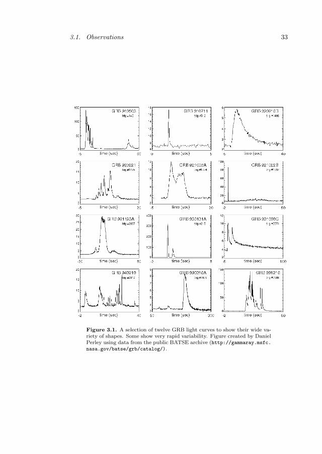
3.1. Observations 33
Figure 3.1. A selection of twelve GRB light curves to show their wide va-riety of shapes. Some show very rapid variability. Figure created by DanielPerley using data from the public BATSE archive (http://gammaray.msfc.nasa.gov/batse/grb/catalog/).
34 Chapter 3. GRB physics
that for most of that time there was no observed emission. Regardless ofthe drawbacks of the T90-parameter, it was realized in the BATSE-era thatthe T90-distribution of GRBs was bimodal (Kouveliotou et al., 1993). Thatis, the sample of GRBs could be subdivided into short GRBs, with a meanduration of ∼ 0.3 s, and long GRBs, with a mean duration of ∼ 26 s. Theseparation between the two populations occur at roughly 2 s. Kouveliotouet al. (1993) also showed that the two population had different hardnessratios: short GRBs were harder than long GRBs. This also supported thehypothesis that they were indeed two separate classes of transients.
It has now been firmly established that the two types of GRBs are associ-ated to different progenitors. Long GRBs have been observed in coincidencewith SN explosions of type Ib/c (Galama et al., 1998; Hjorth et al., 2003;Campana et al., 2006; Pian et al., 2006; Starling et al., 2011; D’Elia et al.,2018), while the famous event GRB 170817A confirmed that at least someshort GRBs are created between the merger of two neutron stars (Abbottet al., 2017a,b). Note that short GRBs may be created in neutron star-blackhole mergers as well (Mochkovitch et al., 1993).
3.1.3 Spectra
GRB spectra are commonly fitted with phenomenological functions such asa cutoff power-law function (CPL) or the Band function (Band et al., 1993).These functions are similar in that they both have a low-energy power-lawslope, α, and a break energy in the spectrum, Epeak. However, they differ intheir behavior at high energies, where the CPL function has an exponentialcutoff while the Band function has an additional high-energy power law withslope β. Often both the models give satisfactory fits to the data, suggestingthat the data at higher energies is not good enough to distinguish betweenthe models. Commonly then, the low-energy slope is used when trying todistinguish between models as the data quality is best at the low-energyend. When GRBs are studied quantitatively using empirical models thedistribution found for the low-energy slope is often a quite smooth curvecentered around α ∼ −1, see figure 3.2.
While these functions usually give satisfactorily fits to the observed emis-sion, they do not tell us about the physical processes involved as they arepurely empirical. Furthermore, the fitted parameters obtained can be mis-leading due to how GRB prompt observations are made. A GRB detectormeasures a count when one of the onboard detectors registers some energydeposit. The count is chategorized into a specific energy bin dependingon how much energy was deposited. However, the detector may not havecompletely stopped the photon, which means that a registered count couldcorrespond to only a fraction of the original photons energy. To convert the
3.1. Observations 35
counts and bins into the information that we want, (i.e., how much energywas deposited during a certain amount time at a certain frequency) one usesa forward-folding technique.
Forward-folding works as follows. First, a model spectrum to mimicthe true spectrum of the source is chosen. Such a model spectrum is forinstance the CPL function or the Band function with specified functionparameters. The model spectrum is then run through the response matrixof the detector. The response matrix outputs a prediction of the number ofcounts in each bin one would observe given that the incoming spectrum wasthe model spectrum. One can then make a statistical comparison of thisoutput to the actual data. The process can then be repeated with slightlydifferent parameter values to see if a better fit is obtained. By iteratingthrough possible parameter combinations, one can find a best fit. However,such a fit relies on the original choice of model spectrum and the best fitparameters could have been different for a different model. The big caveatis that different models, with different physical interpretations, can giveequally good fits to the data once forward folded. Unfortunately, this isthe only way the data can be analyzed, since the response matrix of thedetectors are non-invertable (e.g., Pe’er, 2015).
Several studies have found specific GRBs when a single Band function isnot enough to explain the spectrum, i.e., the spectrum has more complexity.This has been modeled by an additional blackbody component in the X-raysor by an additional break at low or high energies (e.g., Barat et al., 1998;Ryde, 2005; Guiriec et al., 2011; Ryde et al., 2010, 2011; Axelsson et al.,2012; Vianello et al., 2018; Ravasio et al., 2018, 2019; Oganesyan et al.,2019). Interestingly enough, these specific GRBs are commonly very bright.This might suggest that most or all GRB spectra are more complex thanwe think, but that these features are only visible if the data is of sufficientquality.
3.1.4 Low-luminosity GRBs
In 1998, Galama et al. (1998) reported a SN in the error box region of GRB980425. They estimated the chance coincidence of the two events occurringso close to each other in space and time to be less than 1 in 104. Thus, thetwo events were most likely correlated. This was the first time an associationbetween GRBs and SN had been observed. Furthermore, while the GRBseemed common enough in itself, once the very short distance to the eventwas determined it was revealed that GRB 980425 was roughly four orders ofmagnitude less energetic than typical GRBs (E . 1048 erg) (Galama et al.,1998).
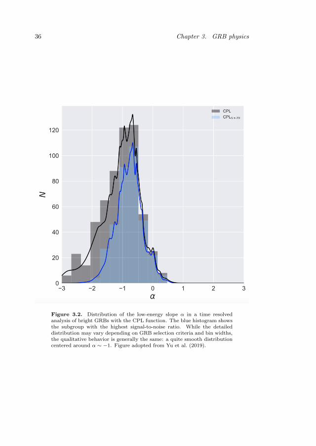
36 Chapter 3. GRB physics
Figure 3.2. Distribution of the low-energy slope α in a time resolvedanalysis of bright GRBs with the CPL function. The blue histogram showsthe subgroup with the highest signal-to-noise ratio. While the detaileddistribution may vary depending on GRB selection criteria and bin widths,the qualitative behavior is generally the same: a quite smooth distributioncentered around α ∼ −1. Figure adopted from Yu et al. (2019).
3.1. Observations 37
With time, more and more detections similar to GRB 980425 were made(e.g., GRB 031203 (Sazonov et al., 2004), GRB 060218 (Campana et al.,2006; Pian et al., 2006), GRB 100316D (Starling et al., 2011)). All of thesewere very close by, associated with luminous SN type Ib/c, and all of themwere much less luminous than standard high-luminosity GRBs. With moredetections, the idea emerged that the low-luminosity GRBs (llGRBs) mightbe a separate class of transients, intrinsically different than the previouslyknown high-luminosity GRBs. One of the compelling arguments for this ideawas that the rate of llGRBs seemed higher than the rate of canonical, high-luminosity GRBs. The lower luminosities of llGRBs mean that they are onlydetectable in a small volume in our local universe, unlike canonical GRBsthat can be seen from incredible distances. Thus, even though detectionsof llGRBs are much more scarce than canonical GRBs, their intrinsic ratecan still be higher. Indeed, rate estimates seem to indicate that llGRBs areat least ten times more common, indicating that the two classes may havedifferent origins (Pian et al., 2006; Soderberg et al., 2006; Guetta & DellaValle, 2007; Sun et al., 2015, see also Section 5.4).
llGRBs are generally believed to be mildly relativistic outflows withbulk Lorentz factors in the order of a few (Soderberg et al., 2006). If theylaunch a jet similarly to high-luminosity GBRs or not is uncertain (Campanaet al., 2006; Fan et al., 2006; Toma et al., 2007). One interpretation ofllGRB prompt emission is that it is caused by a shock breakout from theprogenitor star. In a SN explosion, fast material is launched outwards frominner parts of the parent star generating a shock wave. A shock wave canalso be produced when a jet (succesfuk or choked) drills through a star,creating an energetic cocoon surrounding the jet. As the shock travels fasterthan the speed of sound, the outer layers of the star are initially unawareand unaffected by the internal explosion taking place. A shock breakoutis when the internal shock wave reaches the outer boundary of the star,resulting in flash of X-ray radiation. That llGRBs can be the signature ofa mildly relativistic shock breakout has been advocated by several authors(e.g., Campana et al., 2006; Waxman et al., 2007; Nakar & Sari, 2012).
3.1.5 Afterglow
The material surrounding the GRB explosion is called the circumburstmedium. The GRB jet continuously drills through the circumburst mediumas it propagates. Similarly to a snow plow, the circumburst material isswept up by the jet. The circumburst medium is not very dense so the jetcan reach large distances before it is affected but in the end, inevitably, ithas to slow down. In the framework of the fireball model, the radius at
38 Chapter 3. GRB physics
which the jets starts to decelerate occurs once the swept-up mass energy iscomparable to E/Γ2 (Rees & Meszaros, 1992)
E =4πr3
dec
3ρcbmc
2Γ2, (3.1)
where rdec is the deceleration radius of the outflow and ρcbm is the massdensity of the circumburst medium.
Deceleration radius
An intuitive way of arriving at Equation (3.1) is as follows. Thetotal observed energy of the relativistic flow is E = ΓMc2, whereM is the total mass of the outflow. The total energy in the restframe of the outflow is just the mass energy E′ = Mc2 or E′ = E/Γ.In the outflow frame, the stationary outflow is continuously beingbombarded by incoming particles with an energy density of Γρcbmc
2.The outflow will be unperturbed until the pile up of incoming energyhas become comparable to the rest mass of the outflow. At this point,the outflow starts to be ”dragged along” by the incoming particles(i.e., decelerated in the observers frame). Accounting for the totalswept up volume once the deceleration occurs of 4πr3
dec/3, we obtainEquation (3.1).
The head of the jet creates a forward shock that pushes into the cir-cumburst medium. The shock dissipates the kinetic energy of the outflowand converts it into internal energy in the downstream. The electrons inthe downstream radiate this excess energy as synchrotron radiation. Whena large enough amount of material has been swept up, the synchrotronemission should be visible. Rees & Meszaros (1992) suggested this externalshock radiation as an explanation for the prompt emission, which most peo-ple today believe it is not (although, see Burgess et al., 2016; Acuner et al.,2020). However, Rees & Meszaros (1992) also realized that even if it wasnot responsible for the prompt emission, it should nonetheless exist. Fiveyears later, the afterglow emission was first observed (Costa et al., 1997).
The afterglow is a very important part of a GRB. First of all, it gavecredit to the fireball model as the existence of the afterglow was predictedin the model before the observations were made. Apart from that, theafterglow has the advantage that it lasts much longer than the promptemission. This makes the GRB easier to study with various other differentdetectors. For instance, optical information from the afterglow and theGRB host galaxy can give us the distance to the burst through redshiftdetermination. The afterglow can also give us information regarding the
3.2. Fireball model 39
total energy of the burst, the opening angle, and the Lorentz factor of theoutflow.
Once the jet has piled up enough material, it starts to decelerate sub-stantially. This means that the Lorentz factor of the outflow decreases,which has several consequences. One is that the emitted radiation becomesless Doppler boosted and the observed radiation is therefore less blueshifted.Thus, the observed spectrum is shifted towards lower and lower energies.Another consequence of decreasing Lorentz factor is that the beaming be-comes less significant. Recall (see Section 2.1) that most emission from arelativistically moving object is emitted into a solid cone of opening angleθ ∼ 1/Γ. With decreasing Γ, an observer is able to see emission from largerangles to her line of sight. Thus, the decrease in flux due to the decreas-ing Doppler boost is somewhat counteracted by an increase in flux as theobserver is viewing a larger portion of the jet. At some point in the jet evo-lution however, 1/Γ will become larger than the jet opening angle. Whenthis occurs, the observer is able to see emission from the whole jet at thesame time. After this point, there is nothing to counteract the decrease dueto lower Doppler boost and the flux starts dropping more rapidly with time.This is an important concept in afterglow theory called the jet break, namedafter the break it creates in the light curve. That GRB afterglows exhibitjet breaks indicates that the original outflow was collimated. From the jetbreak, the opening angle of the jet and whether the burst was viewed on oroff axis can be deduced.
3.2 Fireball model
3.2.1 General evolution
GRBs are commonly described in the context of a relativistic fireball (Cav-allo & Rees, 1978; Paczynski, 1986; Goodman, 1986; Rees & Meszaros, 1992;Piran et al., 1993; Rees & Meszaros, 1994; Daigne & Mochkovitch, 1998).Initially, there is a huge release of gravitational energy concentrated into asmall region surrounding the central engine. The incredibly energy densityis quickly converted into a hot plasma with radiation, relativistic pairs, andsome initial baryons. Due to the high pressure, the fireball expands andaccelerates outwards. The expansion continues until most of the availableinternal energy has been converted into bulk kinetic energy of the outflow,at which point the acceleration stalls and the fireball coasts with a constantvelocity.
Consider a central engine that emits a burst of energy with isotropicluminosity L. The luminosity leads to an accelerating outflow, in whichthere are a total of N baryons corresponding to an isotropic mass flux M .
40 Chapter 3. GRB physics
The acceleration continues until all internal energy has been converted intokinetic energy of the bulk outflow. Using thermodynamic arguments, onecan show that the Lorenz factor increases linearly with radius as Γ ∝ rduring the acceleration phase, until the kinetic energy becomes comparableto the total emitted energy once Γ ≈ η = L/Mc2 (e.g., Pe’er, 2015). Thefactor η is called the specific entropy per baryon. From this consideration,one sees that transition radius between the acceleration and coasting phaseis given by
rs = r0η
Γ0, (3.2)
where r0 and Γ0 are the distance from the central engine and Lorentz factorat the base of the acceleration phase. With this definition, one gets a fireballLorentz factor profile
Γ(r) =
Γ0
rr0
if r < rs,
η if r > rs.(3.3)
The outflow accelerates outwards due to the high radiation pressure.This relies on the ejecta being optically thick (Cavallo & Rees, 1978; Good-man, 1986). However, at some point the ejecta will transition from opticallythick to optically thin. This occurs at the photosphere and it results in aflash of photons, since the radiation can now freely stream to the observer.If the photosphere occurs when the jet is still accelerating or close to thesaturation radius, the photospheric emission is predicted to be very bright(Piran et al., 1993; Daigne & Mochkovitch, 2002; Gottlieb et al., 2019).If the photosphere occurs far out in the coasting phase, then the emissionshould be weak since most of the energy is in the form of bulk kinetic energyof the baryons (Piran et al., 1993). However, this is only true if there isno mechanism that dissipates the kinetic energy below the photosphere (seesection 3.3.3 and Rees & Meszaros, 2005).
3.2.2 Temperature and photon number
With a total number of baryons N in the outflow, it follows from conserva-tion of baryon number flux thatNΓβ must be conserved. Here, both β and Γare functions of r, that is they evolve with the evolution of the fireball as theejecta accelerates outwards. Specifically, we have that 4πr2nmΓβdr = dM ,where m is the baryon mass and 4πr2ndr = ndV = dN . This gives
4πr2c nmΓβ = M. (3.4)
Conservation of momentum flux gives that 4πr2hnmc2Γ2βdr = dE, whereh = 1 + 4p/nmc2 is the specific enthalpy and dE = Ldt. This gives
4πr2chnmc2Γ2β = L. (3.5)
3.2. Fireball model 41
Given that L and M are constant during the emission burst period, thetwo equations above imply that hΓ is conserved. Furthermore, it equalshΓ = L/Mc2 = η 1.
In the early phases of the fireball, Γ = Γ0 & 1. Due to the high opticaldepth (e.g., Goodman, 1986; Piran et al., 1993) the radiation and plasma isin thermodynamic equilibrium (see section 3.3.1). The pressure is given byp0 ≈ aT 4
0 . With 4p0/n0mc2 1, one gets
16πr2c aT 40
n
n0Γ0Γβ ≈ L. (3.6)
Evaluating everything in the initial phases of the GRB, one gets
T0 =
(L
16πr20caΓ2
0β0
)1/4
. (3.7)
With a luminosity of L = 1052 erg, an initial radius of r0 ∼ 107 cm, andapproximating Γ2
0β0 ≈ 1, one gets an initial temperature of kT0 ∼ 1 MeV.
The initial temperature is higher than the electron rest mass energy.Thus, the fireball contains radiation and a hot pair-plasma and expandsoutwards due to the internal pressure. When the fireball expands, it coolsand the pairs recombine into photons. An estimate of the number of photonsthe fireball contains per initial baryon after the pairs have recombined canbe obtained as follows. The initial pressure can also be written as theparticle pressure. With an outflow dominated by radiation and pairs, theparticle pressure is approximately p0 ≈ (nγ,i + n±,i)kT0. With h0Γ0 = ηand 4p0/n0mc
2 1 one gets
nγ,i + n±,i ≈ηn0mc
2
4Γ0kT0. (3.8)
Assuming that no more pairs are created, the photon number density atlater times will equal above (accounting for the drop in density due to theexpanding fireball). Specifically, the ratio of photon number density tobaryon number density will be given by (nγ,i+n±,i)/n0 even at later times.Thus,
n =nγ,iz + n±,i
n0=
ηmpc2
4Γ0kT0. (3.9)
With η ∼ 300, mpc2 ≈ 1 GeV, and kT0 ∼ 1 MeV, we see that n ∼ 105. That
means that a GRB jet is dominated by radiation. This is the motivationwhy subphotospheric shocks in GRB jets are photon rich (see section 4.3).
42 Chapter 3. GRB physics
3.2.3 Internal collisions
Once the relativistic fireball has reached the coasting phase, most of theinitial energy is contained in kinetic energy of the relativistic bulk motion.Therefore, all GRB prompt models that rely on emission after the acceler-ation phase need to find a mechanism to transform the kinetic energy intothe observed high-energy radiation. The most commonly discussed mecha-nism is internal collisions (Rees & Meszaros, 1994; Kobayashi et al., 1997;Daigne & Mochkovitch, 1998). The initial burst of energy that launchesthe fireball occurs during some finite amount of time. It is quite plausiblethat the central engine activity varies over that timescale. Furthermore, thejet needs to drill through either a stellar envelope or ejected neutron starmaterial, which may cause variations in the jet flow (Gottlieb et al., 2019).If the variations are such that a latter portion of the jet travels at a muchgreater speed than a former portion, then this may lead to internal colli-sions within the jet. The collisions induce shocks that tap into the kineticenergy and can reprocess it into radiation.
The collisions can occur either in the optically thick or in the opticallythin parts of the jet. If the collisions occur in the optically thin parts, thisleads to a collisionless shock that accelerate particles, which in turn radiatesynchrotron emission. If the collision instead occur in the optically thickparts, the shock becomes a radiation mediated shock and the increasedinternal energy is radiated later at the photosphere. One can estimate thecollision radius as follows.
From the discussion above we know that the dynamical evolution of afireball is acceleration with Γ(r) ∝ r up to the fireball saturation radiusrs = r0η/Γ0, after which the shell coasts and proceeds with a constantΓ = η (see equation (3.3)). The time it takes to reach the saturation radiusts is calculated as
ts =
∫ rs
r0
dr
v(r)=
∫ rs
r0
dr
cβ(r)=
∫ rs
r0
dr
c√
1− 1/Γ(r)2=
∫ rs
r0
rdr
c√r2 − r2
0/Γ20
1
c
[√r2 − r2
0/Γ20
]rsr0
=1
c
[r0
Γ0
√η2 − 1− r0
Γ0
√Γ2
0 − 1
]≈ rs
c,
(3.10)
where the last is true for η 1. Imagine a slower and a faster fireballwith isotropic equivalent luminosities Ls and Lf that are launched with atime separation of δt. If we define t∗ as the time when the second shell hasreached the saturation radius, that is t∗ = δt + ts,f , then for times t > t∗the evolution for both shells is just constant coasting. At time t∗, the rearof the first shell has been coasting for a time t∗ − ts,s with velocity cβs.
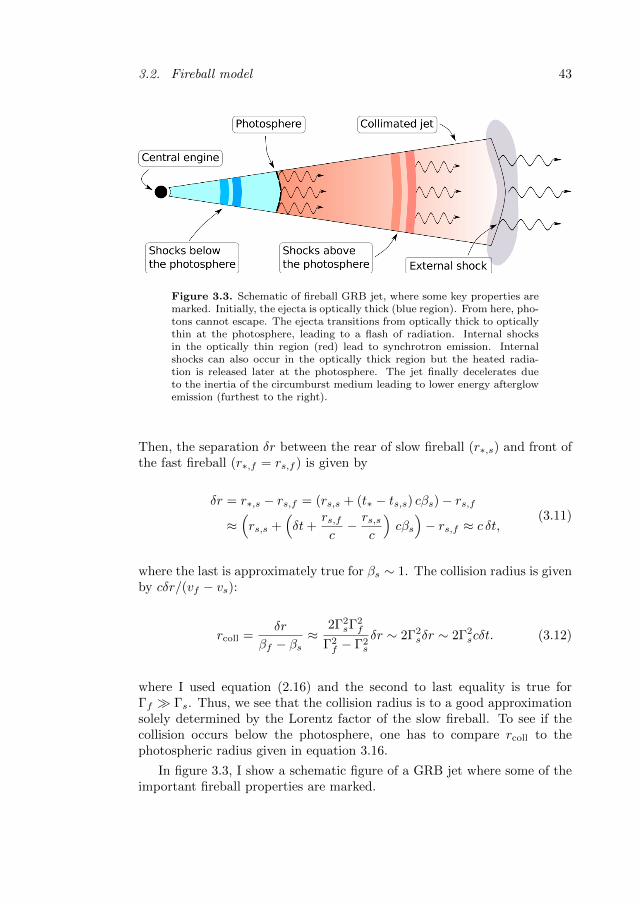
3.2. Fireball model 43
Figure 3.3. Schematic of fireball GRB jet, where some key properties aremarked. Initially, the ejecta is optically thick (blue region). From here, pho-tons cannot escape. The ejecta transitions from optically thick to opticallythin at the photosphere, leading to a flash of radiation. Internal shocksin the optically thin region (red) lead to synchrotron emission. Internalshocks can also occur in the optically thick region but the heated radia-tion is released later at the photosphere. The jet finally decelerates dueto the inertia of the circumburst medium leading to lower energy afterglowemission (furthest to the right).
Then, the separation δr between the rear of slow fireball (r∗,s) and front ofthe fast fireball (r∗,f = rs,f ) is given by
δr = r∗,s − rs,f = (rs,s + (t∗ − ts,s) cβs)− rs,f
≈(rs,s +
(δt+
rs,fc− rs,s
c
)cβs
)− rs,f ≈ c δt,
(3.11)
where the last is approximately true for βs ∼ 1. The collision radius is givenby cδr/(vf − vs):
rcoll =δr
βf − βs≈
2Γ2sΓ
2f
Γ2f − Γ2
s
δr ∼ 2Γ2sδr ∼ 2Γ2
scδt. (3.12)
where I used equation (2.16) and the second to last equality is true forΓf Γs. Thus, we see that the collision radius is to a good approximationsolely determined by the Lorentz factor of the slow fireball. To see if thecollision occurs below the photosphere, one has to compare rcoll to thephotospheric radius given in equation 3.16.
In figure 3.3, I show a schematic figure of a GRB jet where some of theimportant fireball properties are marked.
44 Chapter 3. GRB physics
3.3 Photospheric emission
Initially when the ejecta is launched, the outflow is optically thick, whichmeans that the photons are trapped in the outflow and cannot escape tothe observer (see section 2.2). The photons interact with the particles inthe plasma and tend towards a thermodynamical equilibrium. As the out-flow moves further out, the jet it expands. Thus, the particle density dropsleading to a larger mean separation between the particles. At some point inthe evolutions of the jet, photons will make their last scattering after whichthey freely escape into the Universe for us to see. This results in an ob-served burst of radiation called photospheric emission. To characterize thistransition, one defines a photospheric radius, rph. The photospheric radiusis defined as the radius from the central engine where the optical depth fora photon trapped in its fluid element traveling towards the observer dropsbelow unity.
The photospheric radius can be estimated as follows. The optical depthfor a photon in a fluid element from radius r to an observer at infinity isgiven by (see equation (2.17) and, e.g., Pe’er, 2015)
τ =
∫ ∞r
nσΓ(1− β)dr, (3.13)
where the factor Γ(1 − β) accounts for the fact that interactions are sup-pressed in a beamed outflow and we assume that photons have been emittedto the line of sight. Using the approximation 1− β = 1/2Γ2 from equation(2.15), one gets
τ =
∫ ∞r
nσ
2Γdr. (3.14)
Since we are in the coasting phase, Γ is constant and can be taken outsideof the integral. The density can be estimate from equation (3.5) as n =L/(4πr2mc3Γ2) where both h, β ≈ 1 in the coasting phase. Assuming thecomoving photon energy is below the electron rest mass, one can use theThomson cross section. Integrating from the photospheric radius to infinitygives an optical depth of unity by definition, and thus
1 =LσT
8πmc3Γ3
∫ ∞rph
1
r2dr, (3.15)
which gives the photospheric radius as
rph =LσT
8πmc3Γ3. (3.16)
3.3. Photospheric emission 45
3.3.1 Blackbody radiation
If photons are confined to a plasma for long enough time, they will reacha thermodynamical equilibrium where there is no longer any change to thephoton distribution. In this case, the spectrum is thermal and can be de-scribed by a temperature. Specifically, the spectral shape for a photon dis-tribution in hydrodynamical equilibrium is given by a Planck function andthe radiation is called blackbody radiation.1 Early models of photosphericemission predicted that the observed spectrum would be a Planck function,since the photons would have more than enough time in the optical thickregions to reach a thermal equilibrium (Paczynski, 1986; Goodman, 1986).
Blackbody radiation have a very characteristic form, which is given bythe Planck function:
NE =2ν2
c21
ehν/kT − 1, (3.17)
where NE is photon number flux per energy dN/dE, k is Boltzmanns con-stant and T is the temperature in Kelvin. The spectrum is quite narrow withmost photons energies centered around the temperature. Furthermore, thelow-energy slope is very hard with α = 1, called the Rayleigh-Jeans limit.However, as described in section 3.1.3, this is a poor match for most observedGRB spectra, which are generally broad with α ∼ −1. Thus, photosphericmodels were largely ignored for many years in favor of synchrotron models(see section 3.4). However, around the start of the century, some obser-vation showed very hard GRB spectra consistent with blackbody radiationphotospheric models (Crider et al., 1997; Ghirlanda et al., 2003). Specifi-cally, Ryde (2004) showed that many GRBs could be better fitted when oneallowed for an additional blackbody component along with a non-thermalemission component. These discoveries led to the revival of photosphericmodels, with a lot of new theoretical effort.
3.3.2 Broadening effects: non-dissipative photosphericspectrum
One of the things that was realized was that a photospheric spectrum froma GRB would never be observed as blackbody radiation, as there are severaleffects that will broaden the observed spectrum. Due to the relativistic ve-locities of the outflow, the intrinsic blackbody spectrum has to be Lorentztransformed into the observer frame, increasing the spectral width (Be-loborodov, 2010). If the photosphere occurs already during the acceleration
1For the photons to reach a Planck function, it is necessary that photons can becreated and destroyed. If no photons are generated, the photon distribution is describedby a Wien spectrum, which is a photon distribution in thermal equilibrium with non-zerochemical potential (Rybicki & Lightman, 1979).
46 Chapter 3. GRB physics
phase, this is main effect broadening the spectrum. In this case, Acuneret al. (2019) found that the shape of the spectrum is approximately givenby a cutoff power-law function of the form (see also Ryde et al., 2017)
NE = K
(E
Epivot
)0.66
e−E/Ec (3.18)
where K is a constant, E is observed photon energy Epivot is the pivotenergy, and Ec is the cutoff energy.
Apart from relativistic effects, there are also geometrical effects thatbroaden the spectrum. Firstly, the notion of a photospheric radius is asimplification. The escape of a photon is a probabilistic process, whichmeans that photons escape at a variety of radii. Indeed, the emission occursover more than an order of magnitude in radius (Pe’er, 2008; Lundman et al.,2013). When the radius increases, the outflow cools adiabatically and thetemperature drops. When the outflow is in the acceleration phase, the dropin temperature is cancelled by the increased Lorentz boost. However, whenthe jet is in the coasting phase, this turns the observed spectrum into asuperposition of blackbodies with different temperatures.
Secondly, photons emitted at different angles to the line of sight alsobroaden the spectrum. Photons emitted at larger angles have lower Dopplerboosts, see equation 2.4. Additionally, the optical depth towards the ob-server is angle dependent, again leading to different temperature blackbodiesbeing emitted (Abramowicz et al., 1991; Pe’er, 2008; Lundman et al., 2013).These two effects mean mean that the photosphere is a volume rather thana radius. A spectrum consisting of many different temperature blackbodiesis often called a multicolored blackbody. Accounting for both the relativisticand geometrical effects, Acuner et al. (2019) found that the expected ob-served spectrum from a photosphere in the coasting phase is approximatelygiven by (see also Ryde et al., 2017)
NE = K
(E
Epivot
)0.4
e−(E/Ec)0.65
. (3.19)
These broadening effects are unavoidable in relativistic jets; it is simplyrelated to Lorentz transformations and geometrical effects of the originalfireball photons. As there is no additional energy dissipation below thephotosphere inovoked, such a system is called a non-dissipative photosphere(NDP). In figure 3.4, the NDP spectrum from a photosphere in the accel-eration phase and in the coasting phase as given in equations (3.18) and(3.19) are shown. The spectra are shown compared to a Planck functionand a dissipative photospheric spectrum (see next section).
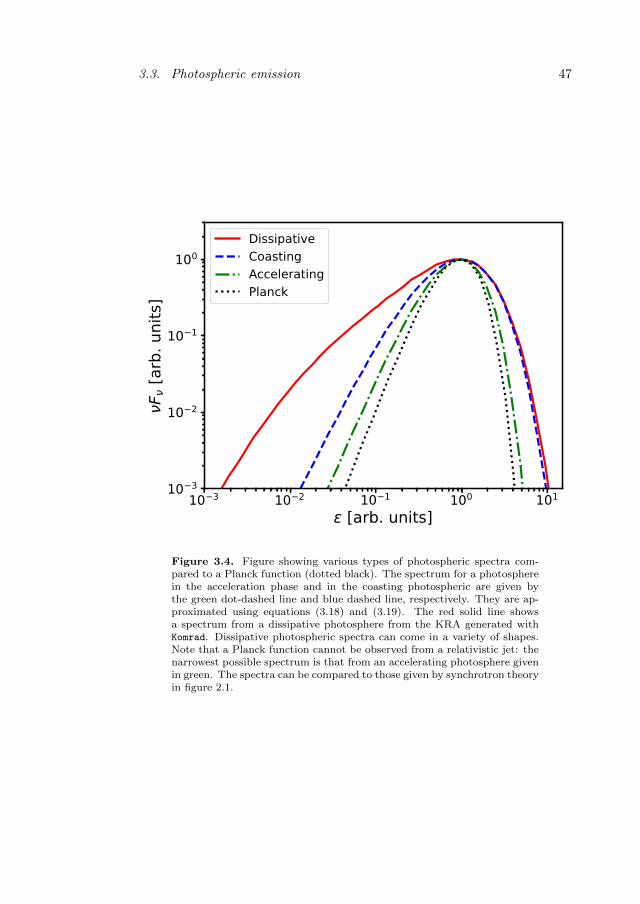
3.3. Photospheric emission 47
10 3 10 2 10 1 100 101
[arb. units]10 3
10 2
10 1
100
F [a
rb. u
nits
]
DissipativeCoastingAcceleratingPlanck
Figure 3.4. Figure showing various types of photospheric spectra com-pared to a Planck function (dotted black). The spectrum for a photospherein the acceleration phase and in the coasting photospheric are given bythe green dot-dashed line and blue dashed line, respectively. They are ap-proximated using equations (3.18) and (3.19). The red solid line showsa spectrum from a dissipative photosphere from the KRA generated withKomrad. Dissipative photospheric spectra can come in a variety of shapes.Note that a Planck function cannot be observed from a relativistic jet: thenarrowest possible spectrum is that from an accelerating photosphere givenin green. The spectra can be compared to those given by synchrotron theoryin figure 2.1.
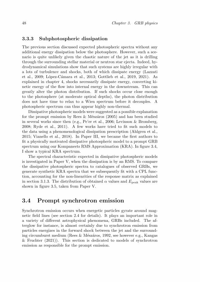
48 Chapter 3. GRB physics
3.3.3 Subphotospheric dissipation
The previous section discussed expected photospheric spectra without anyadditional energy dissipation below the photosphere. However, such a sce-nario is quite unlikely given the chaotic nature of the jet as it is drillingthrough the surrounding stellar material or neutron star ejecta. Indeed, hy-drodynamical simulations show that such systems are highly irregular witha lots of turbulence and shocks, both of which dissipate energy (Lazzatiet al., 2009; Lopez-Camara et al., 2013; Gottlieb et al., 2019, 2021). Asexplained in chapter 4, shocks necessarily dissipate energy, converting ki-netic energy of the flow into internal energy in the downstream. This cangreatly alter the photon distribution. If such shocks occur close enoughto the photosphere (at moderate optical depths), the photon distributiondoes not have time to relax to a Wien spectrum before it decouples. Aphotospheric spectrum can thus appear highly non-thermal.
Dissipative photospheric models were suggested as a possible explanationfor the prompt emission by Rees & Meszaros (2005) and has been studiedin several works since then (e.g., Pe’er et al., 2006; Levinson & Bromberg,2008; Ryde et al., 2011). A few works have tried to fit such models tothe data using a phenomenological dissipation prescription (Ahlgren et al.,2015; Vianello et al., 2018). In Paper III, we became the first authors tofit a physically motivated dissipative photospheric model to a prompt GRBspectrum using our Kompaneets RMS Approximation (KRA). In figure 3.4,I show a typical KRA spectrum.
The spectral characteristic expected in dissipative photospheric modelsis investigated in Paper V, when the dissipation is by an RMS. To comparethe dissipative photospheric spectra to catalogues of observed GRBs, wegenerate synthetic KRA spectra that we subsequently fit with a CPL func-tion, accounting for the non-linearities of the response matrix as explainedin section 3.1.3. The distribution of obtained α values and Epeak values areshown in figure 3.5, taken from Paper V.
3.4 Prompt synchrotron emission
Synchrotron emission occurs when energetic particles gyrate around mag-netic field lines (see section 2.4 for details). It plays an important role ina variety of different astrophysical phenomena, GRBs included. The af-terglow for instance, is almost certainly due to synchrotron emission fromparticles energizes in the forward shock between the jet and the surround-ing circumburst medium (Rees & Meszaros, 1992, see however e.g., Kangas& Fruchter (2021)). This section is dedicated to models of synchrotronemission as responsible for the prompt emission.
3.4. Prompt synchrotron emission 49
1.5 2.0 2.5 3.0 3.5 4.0log(Epeak / [keV])
0.0
0.2
0.4
0.6
0.8
1.0
1.2
1.4No
rmal
ized
occu
renc
er0 = 1010 cm
0 = 4Fermi catalogueAll
< log(R)/2
1.50 1.25 1.00 0.75 0.50 0.25 0.00 0.25cpl
0.0
0.5
1.0
1.5
2.0
2.5
Norm
alize
d oc
cure
nce
r0 = 1010 cm0 = 4
Fermi catalogueAll
< log(R)/2
Figure 3.5. Histograms of the peak energy Epeak and low-energy slopeα obtained by fitting a phenomenological CPL function to synthetic KRAspectra. The red sub-histogram show the shocks that have not had timeto reach steady state (see Paper V for details). The orange line shows thehistograms found for the CPL parameters in a time-resolved catalogue ofbright Fermi GRBs during the first four years (Yu et al., 2016). Figuresadopted from Paper V.
50 Chapter 3. GRB physics
3.4.1 Optically thin shocks
When shocks occur in the optically thin regions of a GRB jet, they areso called collisionless. In collisionless shocks, electromagnetic instabilitiesdevelop and the shock is mediated by particle scattering on the microturbu-lences in the induced fields. The result is that the charged particles undergoFermi acceleration and produce a power-law distribution (see section 4.2).The high-energy particles are present in a region with a strong magneticfield, hence, they radiate synchrotron emission. This is in comparison toshocks that occur in the optically thin parts, where it is the photons thatdirectly gain energy by scattering back and forth in the shock.
External shocks, shocks between the jet and the surrounding medium,are one type of optically thin shocks that are a natural expectation expecta-tion of the fireball model. Today, we know that such shocks are responsiblefor the afterglow emission observed. Early on, they were also suggestedas possible explanations for the prompt emission (Rees & Meszaros, 1992),however, as such it has been largely abandoned. Typical values of thedeceleration radius where the emission would occur are rdec & 1016 cm,which is difficult to reconcile with the shortest observed variability times oftv ∼ 10 ms.
More development has gone into an internal shock framework, where theshocks develop inside the jet as a consequence of variations in the jet velocity(Rees & Meszaros, 1994; Kobayashi et al., 1997; Daigne & Mochkovitch,1998, see figure 3.3). These shocks would occur further in (r ∼ 1013 −1014 cm), which better matches the observed variability time. Internalshock models can reproduce several other GRB characteristics, such as thechaotic behavior sometimes observed and the light curve shapes (Daigne& Mochkovitch, 1998). However, synchrotron emission models have a hardtime explaining the low-energy slope of many GRBs.
3.4.2 Low-energy slope
Internal shocks are not very efficient. Typically, less than 15% of the totalenergy released in the explosion can be converted into released radiation(Daigne & Mochkovitch, 1998). However, the efficiency becomes even lowerif the emitters are in the slow cooling regime, as most energy is then lost toadiabatic cooling. However, this has led to the “synchrotron line-of-death”problem. The overly dramatic name refers to the fact that a large fractionof observed GRBs are harder than theoretical synchrotron models predict.The low-energy slope in a synchrotron spectrum from fast-cooling parti-cles is α = −3/2 (Blumenthal & Gould, 1970; Sari et al., 1998). However,Preece et al. (1998) found that observed GRBs commonly have larger values
3.4. Prompt synchrotron emission 51
of α when they are fitted them with the Band function. Thus, where orig-inal photospheric models predicted slopes that were too hard, synchrotronmodels seemed to predict slopes that were too soft.
A lot of work has gone into explaining the hard slopes within the syn-chrotron framework (e.g., hardening of the spectrum through inverse Comp-ton scattering in the Klein-Nishina regime Derishev et al., 2001; Bosnjaket al., 2009; Nakar et al., 2009; Daigne et al., 2011). In Burgess et al. (2020),a physical synchrotron model was fitted directly to GRB observations. Theauthors found that the synchrotron model could provide satisfactory fitseven to a few cases where the Band model fits suggested α values thatwere above the synchrotron line of death. This indicates that one shouldnot rule out a synchrotron origin based on a Band function fit. Overall, oneshould be cautious when drawing physical conclusions from empirical modelfits. Ravasio et al. (2018, 2019) found that fits to bright GRBs were oftenimproved if one allowed for an additional low-energy break in the fittingfunction. When the spectral indices of the two breaks were analyzed, theywere similar to the values expected in synchrotron theory.2
3.4.3 Proton synchrotron emission
Recent work that have fitted GRB data within the synchrotron frameworkconsistently finds that the injection Lorentz factor γm is close to the coolingLorentz factor γc (Ravasio et al., 2018, 2019; Oganesyan et al., 2019; Burgesset al., 2020), i.e., the emitting particles are marginally fast/slow cooling (seesection 2.4.3). When the emitting particles are electrons, this is difficult toreconcile with what we know about GRBs. Specifically, it requires very largeemission radii (∼ 1017− 1019 cm) and very large Lorentz factors (Γ > 103).This led Ghisellini et al. (2020) to suggest that the emitting particles arenot electron but protons.
The main difficulty with the closeness of γm and γc is that electronscool too quickly. As their synchrotron timescale is very short, γc becomestoo small unless the emission occurs far out where the magnetic field isexpected to be lower. This is not a problem if protons are responsiblefor the emission. As evident from equation (2.26), the cooling timescale isproportional to the mass cubed.3 Thus, if protons are the emitting particles,then the radiation could stem from further in where the magnetic fields arestronger and still have γc . γm. However, Florou et al. (2021) found that ifone accounts for emission from the secondaries produced in photohadronicinteractions, the proton synchrotron model requires fine tuning as to notovershoot optical observations, unless the bulk Lorentz factors of the outflow
2Note that this does not guarantee a synchrotron origin, as we show in Paper V.3One factor of m is removed due to the division of E′ = γ′mc2 in the denominator.
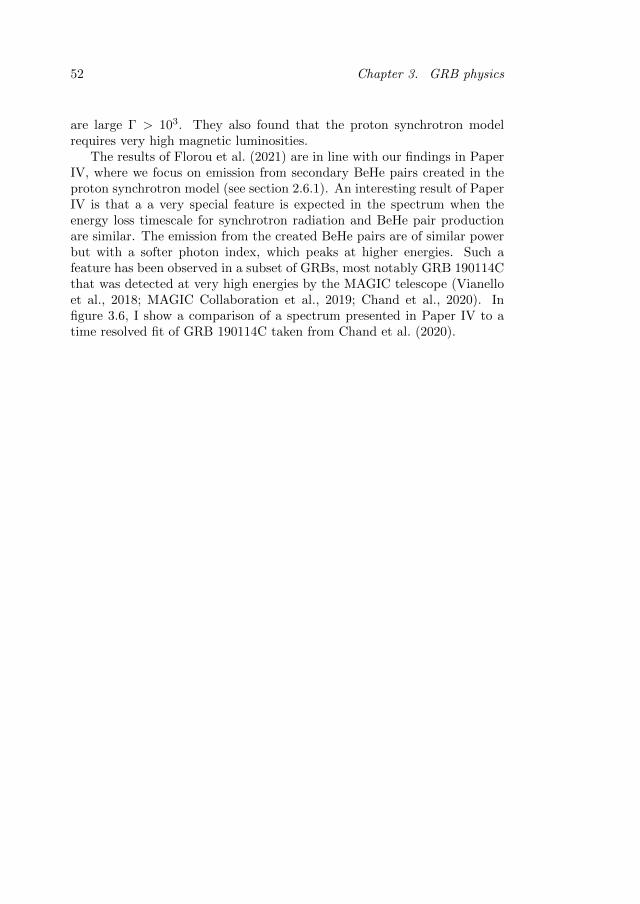
52 Chapter 3. GRB physics
are large Γ > 103. They also found that the proton synchrotron modelrequires very high magnetic luminosities.
The results of Florou et al. (2021) are in line with our findings in PaperIV, where we focus on emission from secondary BeHe pairs created in theproton synchrotron model (see section 2.6.1). An interesting result of PaperIV is that a a very special feature is expected in the spectrum when theenergy loss timescale for synchrotron radiation and BeHe pair productionare similar. The emission from the created BeHe pairs are of similar powerbut with a softer photon index, which peaks at higher energies. Such afeature has been observed in a subset of GRBs, most notably GRB 190114Cthat was detected at very high energies by the MAGIC telescope (Vianelloet al., 2018; MAGIC Collaboration et al., 2019; Chand et al., 2020). Infigure 3.6, I show a comparison of a spectrum presented in Paper IV to atime resolved fit of GRB 190114C taken from Chand et al. (2020).
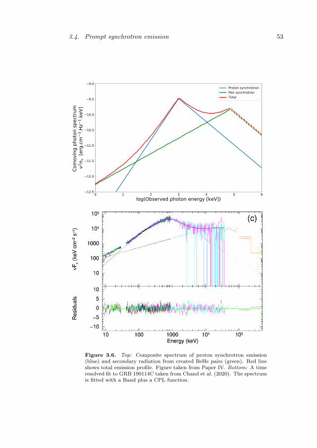
3.4. Prompt synchrotron emission 53
0 1 2 3 4 5 6
log(Observed photon energy [keV])
12.5
12.0
11.5
11.0
10.5
10.0
9.5
9.0
Com
ovin
g p
hoto
n s
pect
rum
2n
[erg
.cm
3.H
z1.k
eV
]
Proton synchrotron
Pair synchrotron
Total
Figure 3.6. Top: Composite spectrum of proton synchrotron emission(blue) and secondary radiation from created BeHe pairs (green). Red lineshows total emission profile. Figure taken from Paper IV. Bottom: A timeresolved fit to GRB 190114C taken from Chand et al. (2020). The spectrumis fitted with a Band plus a CPL function.

54
Chapter 4
Shock physics
Shocks play important roles in various astrophysical phenomena. They arebelieved to be the cause of high-energy photons, cosmic rays, and neutrinos,thus shaping the observable Universe as we know it. They occur frequentlyas the cosmos is filled with violent phenomena where a lot of energy isreleased and commonly devoid of material to stop the acceleration. Theyare important for all parts of this thesis.
4.1 Shock properties
4.1.1 Nomenclature and conventions
There is some shock specific nomenclature that I will frequently employthroughout the chapter. As such, I outline some of the terms here. Ashock has an upstream and a downstream. Particles in the upstream havenot yet passed through the shock and by definition, they have no notion ofthe incoming shock. Particles in the downstream, conversely, have passedthrough the shock and have increased energy. These terms often refer to thefar up- and downstream, which is to say far enough away from the shockwhere the flow is not directly affected by the detailed dynamics close to theshock transition region.
One almost exclusively work in the rest frame of the shock. Thus, onespeak about, e.g., “decelerating the incoming flow” and “the kinetic energyof particles upstream”. However, the upstream may very well be stationaryin the observer frame, as in the case of external shocks with a constantinterstellar medium described in section 3.1.5, or moving relativistically inthe same direction as the shock, as in the case of internal shocks describedin section 3.2.3.
55
56 Chapter 4. Shock physics
Macroscopically, a shock is a discontinuity of several flow properties.However, the shock does have a width over which the properties vary con-tinuously. The shock width is the deceleration length of the upstream, i.e.,the interaction length it takes to slow down the upstream from its upstreamvelocity, βu, to its downstream velocity, βd.
An important concept in shock physics is the Mach number,M, definedas the ratio of the velocity to the sound speed cs. The shock jump conditionsfor a nonrelativistic shock can be expressed in a very compact way usingthe Mach number of the upstream Mu = vu/cs,u. These jump conditionsand other shock properties simplify greatly in the case of a strong shock,defined as Mu →∞.
4.1.2 Entropy increase
Shocks have many important properties. One of the most important is thatthey transform kinetic energy into heat.
Entropy increase
Consider an ice cube in a room at room temperature. The ice cubewill melt as the heat in the room is transferred from the warmerair to the colder ice cube. The watery remains of the ice cube willnot spontaneously freeze again: the entropy of the isolated ice cubeplus room system has increased. A shock occurs when something fasttravels with supersonic speeds relative to a slow medium. The initialfast material and the swept up slow material travel with the samespeed downstream of the shock. Just like how the ice cube cannotspontaneously freeze again, these two parts cannot spontaneouslybe separated into slower and faster moving material. Entropy hasincreased. The entropy increase comes from the transformation ofkinetic energy into internal energy (heat). Indeed, in the collisionof any two objects with different initial velocities, which afterwardstravel with the same velocity, kinetic energy must always be lost.This can easily be seen by considering conservation of momentum.Imagine one object with mass M and speed v1 and a second objectwith mass m at rest. If they after the collision travel with the same(nonrelativistic) speed, v2, then conservation of momentum impliesthat (M + m)v2 = Mv1. The kinetic energy afterwards is given byEkin,2 = (M + m)v2
2/2 = M2v21/(2(M + m)) = Ekin,1M/(M + m).
As m > 0, the kinetic energy must have decreased. The energy hasbeen converted into heat in the collision. In a similar way, a shockdissipates kinetic energy into internal energy.
4.1. Shock properties 57
4.1.3 Shock jump conditions
A shock wave can macroscopically be seen as a discontinuity in severalshock properties, such as density, velocity, and pressure. However, energyand momentum must still be conserved. In the absence of particle creation,the particle number is also conserved. From this, one can derive the shockjump conditions, which stipulate how much hydrodynamical quantities mustchange when traversing the shock. The following analysis follows closelysection 2.3 in Levinson & Nakar (2020), there given for a radiation mediatedshock. However, it is generally valid for any type of shock under the givenassumptions.
The four velocity of a flow is given by uµ = γ(1,β), which, if the shockis one-dimensional, becomes uµ = γ(1, β). Here, I excluded a factor of ccompared to the from the usual formalism of the four-velocity uµ = cγ(1,β).The energy-momentum tensors (also called the stress-energy tensors) fora neutral baryonic fluid, Tµνb , a pair-fluid, Tµν± , and the radiation, Tµνγ ,assuming negligible magnetic fields and Maxwell-Juttner distributions forelectrons and pairs (justified in the case of a photon rich RMS as the particleare tightly coupled to the radiation) are
Tµνb =
[n(mi +me)c
2 +5
2pi +
(1 +
3
2g(T )
)pe
]uµuν + ηµν(pi + pe),
Tµν± =
[n±mec
2 +
(1 +
3
2g(T )
)p±
]uµuν + ηµνp±,
Tµνγ =
∫kµkνfγ(k, x)
d3k
k0.
(4.1)
Above, n is the baryonic density, assumed equal for the ions and primaryelectrons and ηµν is the Minkowski metric, equal to diag(−1, 1, 1, 1) in flatspacetime. The 5/2pi comes from the fact that the ions are assumed nonrel-ativistic. Indeed, the full expression in the brackets is ei+pi, but with a non-relativistic equation-of-state, ei = 3/2pi. The factor g(T ), derived in Bud-nik et al. (2010), is designed to capture both nonrelativistic and relativisticequations-of-state for the electrons and pairs, depending on the temperatureT . The specific energy is then related to the pressure as ei = 3g(T )pi/2.The temperature of the primary electrons and the pairs are assumed equal(again valid in the case of an RMS due to the strong coupling to the radia-tion field).
For the radiation, kµ = hνc (1, Ω) is the photon four-momentum, where
Ω is the unit direction vector. The fγ(k, x) denotes the phase-space distri-bution function of the radiation. If the radiation is isotropic in the fluid rest
58 Chapter 4. Shock physics
frame, the energy-momentum tensor of the radiation can be approximatedas Tµνγ = 4pγu
µuν + ηµνpγ .Conservation of baryon number, energy, and momentum implies that
∂
∂xµ(nuµ) = 0,
∂
∂xµ(Tµνb + Tµν± + Tµνγ ) = 0.
(4.2)
The derivative notation means you take the time derivative of the time-component of the four vector and the space derivative of the space compo-nent. For the conservation of mass, it implies
∂
∂xµ(nuµ) = ∂t(nγ) + ∂x(nγβ) = 0 (4.3)
If one assumes a steady state, then all time derivatives vanish. If one furtherassumes a planar shock, then the space derivative is in one dimension. Thus,above implies
∂x(nγβ) = 0 → nuγuβu = ndγdβd, (4.4)
where the subscripts u and d refer to quantities evaluated in the far up- anddownstream of the shock, respectfully. If one omits the rest mass density ofthe primary electrons, one gets the conservation of energy and momentum∂∂xµ (Tµνb + Tµν± + Tµνγ ) in steady state as
∂x
[(nmic
2 + n±m±c2 +
5
2pi + 4pγ +
(1 +
3
2g(T )
)(pe + p±)
)γ2β
]= 0
(4.5)in the case when ν = 0 and
∂x
[(nmic
2 + n±m±c2 +
5
2pi + 4pγ +
(1 +
3
2g(T )
)(pe + p±)
)γ2β2 + p
]= 0
(4.6)when ν = 1. Above, the solemn p is the sum of all pressures: p =pi + pe + p± + pγ . These expressions can be simplified with some, oftenvalid, assumptions. In addition to steady state, one commonly assumesnegligible iron pressure, negligible rest mass energy of pairs upstream, andnonrelativistic electrons upstream. Finally, let us consider the scenario of ashock where the electrons are not relativistic and where the photons do notexceed the electron rest mass.1 In this case, pair-production is negligible
1When this is not the case, one has to consider the contribution from pairs and arelativistic equation of state for the electrons downstream.
4.1. Shock properties 59
and the electrons downstream are nonrelativistic. Then, the shock jumpcondition reads
nuγuβu = ndγdβd,(numic
2 + 4pγ,u +5
2pe,u
)γ2uβ
2u + pu =
(ndmic
2 + 4pγ,d +5
2pe,d
)γ2dβ
2d + pd,(
numic2 + 4pγ,u +
5
2pe,u
)γ2uβu =
(ndmic
2 + 4pγ,d +5
2pe,d
)γ2dβd,
(4.7)
where the pressure pi is the sum of radiation and electron pressure as pi =pγ,i+pe,i. Note that hydrodynamical quantities such as pressure and densityis evaluated in the respective rest frame of the plasma, i.e., in the restframe of the far upstream or the far downstream. This is in contrast to theLorentz factors and velocities, which are evaluated with respect to the shockrest frame. The conditions given in equation (4.7) are not only applicableto shocks. They are general statements regarding conservation of particlenumber, momentum, and energy flux.
4.1.4 Speed after relativistic collision
In the internal collision scenario outlined in section 3.2.3, two ultra-relativisticfireballs collide within the GRB jet. The collision launches a forward shocktraveling into the slower fireball and a reverse shock traveling into the fasterone. In between the two shocks is the downstream, which the two shocksshare. As a shock increases the entropy, it is an attractive way to transferkinetic energy back into internal energy and radiation. As a common themein many GRB models, it is of interest to know how fast the shared down-stream travels after a collision (see also Kobayashi et al., 1997; Daigne &Mochkovitch, 1998).
In the stationary frame of the common downstream, the incoming mo-mentum flux from the reverse shock must equal the incoming momentumflux from the forward shock by definition. This gives the equation (cf. mid-dle line equation (4.7))
Γ2sβ
2s (ρsc
2 + es + ps) + ps = Γ2f β
2f (ρfc
2 + ef + pf ) + pf . (4.8)
Here, the bars denote quantities evaluated in the frame of the commondownstream (recall that hydrodynamical quantities are proper, i.e., evalu-ated in their local rest frame). The subscripts s and f refer to the fast and
60 Chapter 4. Shock physics
the slow fireball, respectively. Under the assumption that both upstreamsare cold (es, ps, ef , pf ∼ 0), this simplifies to
Γsβsρ1/2s = Γf βfρ
1/2f . (4.9)
Using equation (2.12), we can transform the relativistic velocities evaluatedin the common downstream frame to observer frame quantities as
(β − βs)ΓsΓρ1/2s = (βf − β)ΓfΓρ
1/2f , (4.10)
where Γ is the observed Lorentz factor of the common downstream andβ =
√1− 1/Γ2, is the associated speed. As Γf > Γ > Γs 1, one can
safely use the Taylor expansion in the last expression of equation (2.12),which gives (
Γ
2Γs− Γs
2Γ
)ρ1/2s =
(Γf2Γ− Γ
2Γf
)ρ
1/2f . (4.11)
Multiplying both sides by 2Γ and separating the terms with Γ2 gives
Γ2
(ρ
1/2s
Γs+ρ
1/2f
Γf
)= ρ1/2
s Γs + ρ1/2f Γf (4.12)
which finally gives
Γ2 =ρ
1/2s Γs + ρ
1/2f Γf
ρ1/2s /Γs + ρ
1/2f /Γf
= ΓsΓfρ
1/2s Γs + ρ
1/2f Γf
ρ1/2s Γf + ρ
1/2f Γs
. (4.13)
If the comoving densities of the two fireballs are equal, ρs = ρf , then theLorentz factor for the common downstream is simply
Γ =√
ΓsΓf . (4.14)
4.2 Diffusive shock acceleration
A core concept that can explain the power-law spectra often observed inastrophysical sources is the theory of diffusive shock acceleration. The ac-celeration is a Fermi type acceleration. The principle idea is that particlesinteract with some high-inertia scatterer and in each elastic scattering, theparticles can either lose or gain energy. If the probability for an interactionwith an energy gain is larger than the probability for an energy loss, thisleads to an average energy increase for the particles. In his original paper,Fermi envisioned clouds of high density magnetic fields that could scattercharged particles. As particles were more likely to encounter approaching
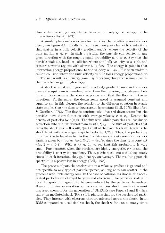
4.2. Diffusive shock acceleration 61
clouds than receding ones, the particles more likely gained energy in theinteractions (Fermi, 1949).
A similar phenomenon occurs for particles that scatter across a shockfront, see figure 4.1. Really, all you need are particles with a velocity vthat scatter in a bulk velocity gradient du/dx, where the velocity of thebulk motion u v. In such a system, the particle can scatter in anygiven direction with the roughly equal probability as v u. Say that theparticle makes a head on collision where the bulk velocity is u + du andscatters towards regions with slower bulk flow. The energy it gains in thatinteraction energy proportional to the velocity u + du. If it then makes atail-on collision where the bulk velocity is u, it loses energy proportional tou. The net result is an energy gain. By repeating this process many times,the particle can gain high energy.
A shock is a natural region with a velocity gradient, since in the shockframe the upstream is traveling faster than the outgoing downstream. Letsfor simplicity assume the shock is planar and that the flow is in the x-direction. Furthermore, the downstream speed is assumed constant andequal to ud. In this picture, the solution to the diffusion equation in steadystate implies that the density downstream is constant (Bell, 1978; Blandford& Ostriker, 1978). The flow is continuously advected downstream but theparticles have internal motion with average velocity v ud. Denote thedensity of particles by n(x, t). The flux with which particles are lost due toadvection into the far downstream is n(x, t)ud. The flux of particles thatcross the shock at x = 0 is n(0, t)v/4 (half of the particles travel towards theshock front with a average projected velocity 1/2v). Thus, the probabilityfor a particle to be advected to the downstream without crossing the shockagain is given by n(x, t)ud/n(0, t)v/4 = 4ud/v, since the density is constantn(x, t) = n(0, t). With ud/v 1, we see that this probability is verysmall. Furthermore, when the particles are highly energetic, v ∼ c and theprobability is energy independent. Thus, particles can cross the shock manytimes, in each iteration, they gain energy on average. The resulting particlespectrum is a power-law in energy (Bell, 1978).
The process of particle acceleration in a velocity gradient is general andnot specific to any type of particle species, as long as it can scatter in thegradient with little energy loss. In the case of collisionless shocks, the accel-erated particles are charged baryons and electrons. The particles scatter inlocal hotspots of magnetic turbulence induced by the particles themselves.Baryon diffusive acceleration across a collisionless shock remains the mostdiscussed scenario for the generation of UHECRs (see Papers I and II). In aradiation mediated shock (RMS) it is photons that are the accelerated parti-cles. They interact with electrons that are advected across the shock. In anRMS compared to a collisionless shock, the shock width can be many times
62 Chapter 4. Shock physics
Figure 4.1. Schematic showing the principle behind diffusive shock accel-eration. Particles scatter with dense patches of magnetic turbulence thatthey themselves generate. The stochastic process lead to a net energy gainevery time they cross the shock front. Figure adopted from Treumann &Jaroschek (2008).
larger than the typical mean free path of the scattering particles. Hence,the photons do not make several crossings of the shock as a whole. However,as evident from the discussion above, it is enough that the photons scatterback and forth in the velocity gradient within the shock to gain energy andform a power-law distribution. RMSs are of central importance in PapersIII and V and are discussed in more detail below.
4.3 Radiation mediated shocks
In regions where the optical depth is high, radiation mediated shocks (RMSs)can occur. Such shocks are less common than collisionless shocks in astro-physical settings but can still be found in a variety of sources. The first lightfrom a supernova (SN) is due to the breakout of an RMS from the stellar en-velope. The short GRB observed in the famous multi-messenger event GRB170817A may very well have been an RMS shock breakout (Bromberg et al.,2018; Gottlieb et al., 2018; Lundman & Beloborodov, 2021). Additionally,they occur in accretion disks around black holes, in low-luminosity GRBs,and in the inner optically thick part of jets. Early studies on RMSs focused
4.3. Radiation mediated shocks 63
terrestrial systems and SNe (Weaver, 1976) and it was not until quite re-cently that one started to realized their importance for other transients aswell, such as GRB jets. This has led to the development of a relativisticframework for RMSs (Levinson & Bromberg, 2008; Bromberg et al., 2011).
In a RMS, Compton scattering between the photons and the plasma iswhat is mediating the shock. Although this is the underlying mechanism forall phenomena listed above, the details differ between the systems. Firstly,an RMS can be either photon poor or photon rich. In a photon poor RMS,the upstream is initially devoid of photons. The photons that mediate theshock are created in the downstream, mostly via Bremsstrahlung emission.In a photon rich shock on the other hand, the creation of photons is dwarfedby the large number of photons already present in the upstream. Here, thephoton number is simply dominated by advection. Secondly, the dynamicsis different if the shock is nonrelativistic, βu . 0.5, or highly relativistic,uu & 3.5. In nonrelativistic shocks, the diffusion approximation is validsince the photon field is isotropic. In highly relativistic shocks, anisotropybecomes prevalent and violent pair production can occur, both of whichwill change the dynamics of the system (Ito et al., 2018; Lundman et al.,2018). In the intermediate regime, relativistic effects have little effect onthe final photon spectrum (see Paper III). Magnetic fields can further alterthe dynamics of the RMS (Lundman & Beloborodov, 2019).
Lundman et al. (2018) found that in photon rich RMSs, the photon dis-tribution resembles a power-law spectrum with an exponential cutoff in theimmediate downstream. The power-law forms due to a Fermi-like processwhere particles scatter back and forth in the shock as explained in section4.2. The generated spectrum is remarkably similar to the photon distribu-tion resulting from photons interacting with thermal electrons as describedby the Kompaneets equation (see section 2.5.2). This is the foundation forPapers III and V. In figure 4.2, I show a comparison between spectra gener-ated by full scale radiation hydrodynamic simulation and the approximatemodel that we developed in Paper III. I also show the fit that we performedin Paper III, which was the first ever RMS model fit to GRB data.
4.3.1 Radiation dominance and interaction scales
A shock is mediated by radiation if two conditions are met. Firstly, thedownstream pressure should be dominated by radiation and secondly, thesystem should be optically thick such that the photons cannot diffuse outbefore they have decelerated the upstream. Following e.g., Levinson &Nakar (2020), one can get an estimate for when these conditions are metas follows. The downstream velocity in the shock rest frame is often quitesmall, as is the pressure upstream. Using the jump conditions from equation
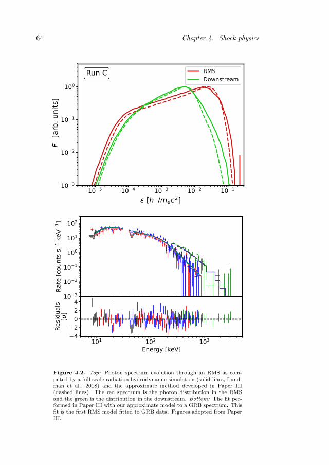
64 Chapter 4. Shock physics
10−5 10−4 10−3 10−2 10−1ε [hν/mec2]
10−3
10−2
10−1
100
νFν [arb. units]
Run C RMSDownstream
10 3
10 2
10 1
100
101
102
Rate
[cou
nts s
1 keV
1 ]
101 102 103
Energy [keV]
42024
Resid
uals
[]
Figure 4.2. Top: Photon spectrum evolution through an RMS as com-puted by a full scale radiation hydrodynamic simulation (solid lines, Lund-man et al., 2018) and the approximate method developed in Paper III(dashed lines). The red spectrum is the photon distribution in the RMSand the green is the distribution in the downstream. Bottom: The fit per-formed in Paper III with our approximate model to a GRB spectrum. Thisfit is the first RMS model fitted to GRB data. Figures adopted from PaperIII.
4.3. Radiation mediated shocks 65
(4.7) with γu = 1, one can estimate the downstream pressure from theconservation of energy density as
numic2β2u ≈ pd. (4.15)
The pressure downstream is from particle pressure and radiation pressure,which, if the plasma is in hydrodynamic equilibrium equals pd = ndkTd +aT 4
d /3, where a is the radiation constant. For radiation pressure to dominatein the downstream, one gets aT 4
d /3 > ndkTd. Solving the inequality for Tdand plugging back into equation (4.15), one obtains
β2u > 2
(ndk)4/3
numic2
(3
a
)1/3
. (4.16)
In a nonrelativistic, strong shock, nd/nu ≈ 7. Using the proton mass formi, one gets a condition for the upstream velocity as
βu > 3× 10⁻⁴ n1/6u,15. (4.17)
Equation (4.17) tells us that a shock starts to become radiation dominatedalready at quite slow shock speeds, with rather weak parameter dependence.
The second condition is that the system is sufficiently optically thick.As the upstream is decelerated by radiation that is diffusing from the down-stream, the shock width can be estimated by equating the radiation diffusiontime by the upstream advection time. Denote the RMS width by L. Thenthe advection time of the upstream with velocity vu across the shock is sim-ply L/vu. The diffusion time is approximately the total distance traveledby a photon diffusing through the shock region divided by c. The distanceis the number of scatterings, N , times the mean free path, λ. From section2.3, we have that N ≈ τ2. Assuming constant density across the RMS, wealso get from section 2.3 that λ ≈ L/τ . Equating the two timescales thegive an estimate of the optical depth across the shock as
τ ≈ c
vu=
1
βu. (4.18)
The optical depth of the system must exceed this value. Otherwise, photonsescape upstream before the upstream is fully decelerated.
Actually, the two conditions above would not have been sufficient if theinteraction length of the plasma particles had been longer than the radiationmean free path. However, a typical length scale for particle interaction is
the plasma skin depth, which for protons and electrons equal 1 n−1/2u,15 cm
and 0.01 n−1/2u,15 cm, respectively. The radiation mean free path on the other
hand is given by λ = 1/nuσT ≈ 1.5 × 109 cm. The incredible difference in
66 Chapter 4. Shock physics
interaction scales imply that simulations that try to resolve both becomeextremely time consuming, which explains why there was a need for anapproximate, faster method, i.e., the KRA (see Paper III).
In a GRB jet, there are ∼ 105 times more photons than there are baryonsand electrons (when the pairs have recombined, see equation (3.9)). RMSsthat occur in GRB jets are therefore photon rich. Furthermore, for eachscattering a photon undergoes, an electron scatters ∼ 105 times. Thus,electrons are to a good approximation in a thermal distribution across theentire shock, as well as in the upstream and downstream regions. Theelectron temperature equals the Compton temperature (see section 2.5.2): ifthe electron population had more (less) energy than the photons on average,they would lose (gain) that excess energy almost immediately.
4.3.2 Jump conditions in RMS with vanishing paircontent
The number of pairs created in an RMS can be substantial if the shockvelocity is large enough (uu & 3, Lundman et al., 2018). Pairs are createdwhen the comoving photon energies exceed the electron rest mass. However,in Paper III we found that an RMS can be treated without accounting forrelativistic effects (pair creation, Klein-Nishina scattering, and anisotropy)as long as εmax < 1, where εmax is the maximum comoving photon energyin units mec
2. In Paper III, we found that the speed limit where this holdsis
u2u .
ξ
ln(εd/εu), (4.19)
where ξ ≈ 55 is a constant and ε is the average photon energy. From above,we find that the speed limit where relativistic factors need to be accountedfor is quite insensitive to the parameter. For a typical value of (εd/εu) = 100,one gets uu . 3.5. Thus, the upstream can be mildly relativistic withoutneeding to account for relativistic effects in the flow.
If equation (4.19) is satisfied, we do not need to account for any pair pro-duction. Furthermore, the downstream pressure is dominated by radiationin an RMS and the pressure upstream can also be assumed dominated byradiation (although this contribution is most likely negligible in comparisonto the proton rest mass energy). In that case, the shock jump conditionsfrom equations (4.7) reads
nuγuβu = ndγdβd,(numic
2 + 4pγ,u)γ2uβ
2u + pγ,u =
(ndmic
2 + 4pγ,d)γ2dβ
2d + pγ,d,(
numic2 + 4pγ,u
)γ2uβu =
(ndmic
2 + 4pγ,d)γ2dβd.
(4.20)
4.3. Radiation mediated shocks 67
The system above can be simplified further by introducing ui = γiβi andwi = 4pi/nimc
2. By dividing the second and third line by numic2uu and
using the fact that nd/nu = uu/ud from the first line, one obtains (see alsoBeloborodov, 2017)
nuuu = ndud,
(1 + wu)uu +wu4uu
= (1 + wd)ud +wd4ud
,
(1 + wu)γu = (1 + wd)γd.
(4.21)
The dimensionless enthalpy, w, when radiation dominates the pressure canbe written as
wi =4pγ,inimc2
=4eγ,i
3nimc2=
4εimec2nγ
3nimc2=
4εimen
3m, (4.22)
where eγ,i is the internal energy in radiation, pi = ei/3 is valid for a rel-ativistic equation of state, and the factor mec
2 appears since ε is given inunits of mec
2. To solve the system of equation above, it is sufficient if oneknows the average photon energy upstream εu, the photon to proton ratio n,and the upstream velocity uu (or, equivalently, βu). Note that this cannottell you the absolute value of the photon densities nd and nu but only theirratio nd/nu.
This is the system of equations we use to determine the downstreamproperties in Paper III and V. In Paper V, the upstream temperature inthe shock frame is not known but must be calculated. This is done usingthe relativistic velocity transformation given in equation (2.11): γu = (1−βfsβs)ΓfsΓs and γd = (1 − βfsβ)ΓfsΓ. Here, Γfs is the bulk Lorentz factorof the forward shock, Γs is the bulk Lorentz factor of the slow fireball, andΓ is the bulk Lorentz factor of downstream, all evaluated in the observerframe (see also Paper V). This introduces one more unknown, Γfs, but withtwo additional equations, the system can be solved.

68
Chapter 5
UHECR physics
The energies of UHECRs are incomprehensible. In the large hadron colliderat CERN, particles are accelerated up to 6.5 TeV (6.5×10¹² eV). The mostenergetic UHECRs reach energies that are more than million times higher.The ratio is the same as the width of a fingernail (. 1 cm) to the height ofMount Everest (. 10 000 m). UHECRs can therefore help us study particlephysics at energies that would be otherwise unattainable.
The chapter is divided as follows. In section 5.1, I give some details tothe observations of UHECRs. Sections 5.2 and 5.3 give constraints on thelocal magnetic field necessary to accommodate UHECR acceleration and insection 5.4, I derive the minimum total energy of possible sources.
5.1 Observations
5.1.1 Detection
Experiments designed to detect UHECRs do not detect the particles di-rectly. When an UHECR enters the atmosphere, it interacts with the densesurrounding. The interactions create secondary particles such as pions, neu-trinos, and gamma-rays (see section 2.6). The large energy of the incomingparticle gets imparted into the secondaries. Thus, these are themselvesenergetic enough to create further particles by e.g., pair production. Theoriginal UHECR thus produce a shower of particles called an extensive airshower. It is the extensive air showers that the experiments detect.
One of the detector types used is water Cherenkov detectors. Theseare used in for instance the Pierre Auger experiment mentioned in section1.2. Water Cherenkov detectors are large water tanks spread out across thedetector area. Each water tank is surrounded by sensitive photomultiplier
69
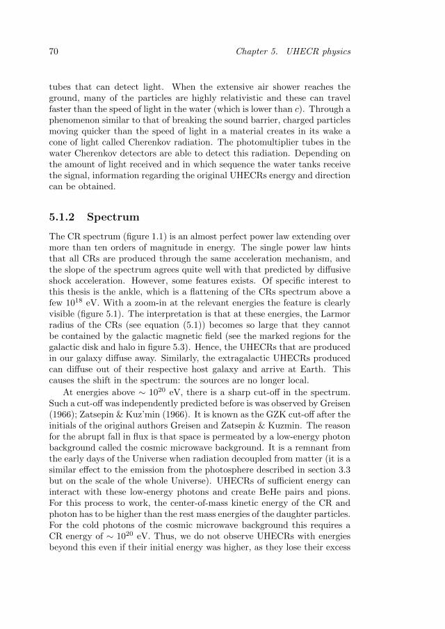
70 Chapter 5. UHECR physics
tubes that can detect light. When the extensive air shower reaches theground, many of the particles are highly relativistic and these can travelfaster than the speed of light in the water (which is lower than c). Through aphenomenon similar to that of breaking the sound barrier, charged particlesmoving quicker than the speed of light in a material creates in its wake acone of light called Cherenkov radiation. The photomultiplier tubes in thewater Cherenkov detectors are able to detect this radiation. Depending onthe amount of light received and in which sequence the water tanks receivethe signal, information regarding the original UHECRs energy and directioncan be obtained.
5.1.2 Spectrum
The CR spectrum (figure 1.1) is an almost perfect power law extending overmore than ten orders of magnitude in energy. The single power law hintsthat all CRs are produced through the same acceleration mechanism, andthe slope of the spectrum agrees quite well with that predicted by diffusiveshock acceleration. However, some features exists. Of specific interest tothis thesis is the ankle, which is a flattening of the CRs spectrum above afew 1018 eV. With a zoom-in at the relevant energies the feature is clearlyvisible (figure 5.1). The interpretation is that at these energies, the Larmorradius of the CRs (see equation (5.1)) becomes so large that they cannotbe contained by the galactic magnetic field (see the marked regions for thegalactic disk and halo in figure 5.3). Hence, the UHECRs that are producedin our galaxy diffuse away. Similarly, the extragalactic UHECRs producedcan diffuse out of their respective host galaxy and arrive at Earth. Thiscauses the shift in the spectrum: the sources are no longer local.
At energies above ∼ 1020 eV, there is a sharp cut-off in the spectrum.Such a cut-off was independently predicted before is was observed by Greisen(1966); Zatsepin & Kuz’min (1966). It is known as the GZK cut-off after theinitials of the original authors Greisen and Zatsepin & Kuzmin. The reasonfor the abrupt fall in flux is that space is permeated by a low-energy photonbackground called the cosmic microwave background. It is a remnant fromthe early days of the Universe when radiation decoupled from matter (it is asimilar effect to the emission from the photosphere described in section 3.3but on the scale of the whole Universe). UHECRs of sufficient energy caninteract with these low-energy photons and create BeHe pairs and pions.For this process to work, the center-of-mass kinetic energy of the CR andphoton has to be higher than the rest mass energies of the daughter particles.For the cold photons of the cosmic microwave background this requires aCR energy of ∼ 1020 eV. Thus, we do not observe UHECRs with energiesbeyond this even if their initial energy was higher, as they lose their excess
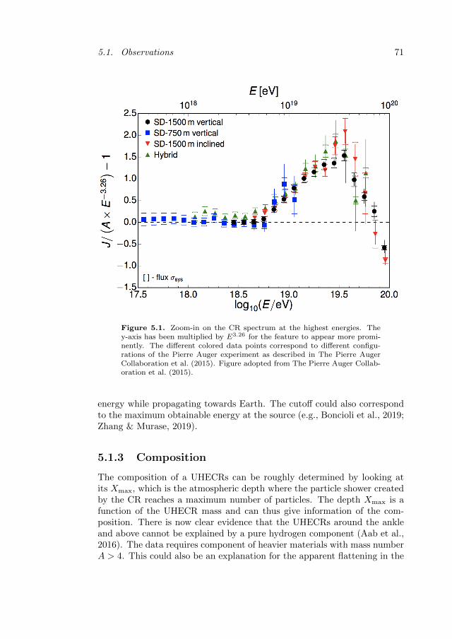
5.1. Observations 71
Figure 5.1. Zoom-in on the CR spectrum at the highest energies. They-axis has been multiplied by E3.26 for the feature to appear more promi-nently. The different colored data points correspond to different configu-rations of the Pierre Auger experiment as described in The Pierre AugerCollaboration et al. (2015). Figure adopted from The Pierre Auger Collab-oration et al. (2015).
energy while propagating towards Earth. The cutoff could also correspondto the maximum obtainable energy at the source (e.g., Boncioli et al., 2019;Zhang & Murase, 2019).
5.1.3 Composition
The composition of a UHECRs can be roughly determined by looking atits Xmax, which is the atmospheric depth where the particle shower createdby the CR reaches a maximum number of particles. The depth Xmax is afunction of the UHECR mass and can thus give information of the com-position. There is now clear evidence that the UHECRs around the ankleand above cannot be explained by a pure hydrogen component (Aab et al.,2016). The data requires component of heavier materials with mass numberA > 4. This could also be an explanation for the apparent flattening in the
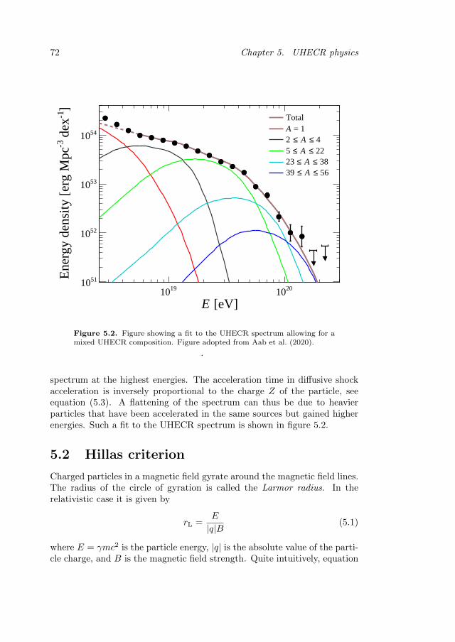
72 Chapter 5. UHECR physics
1910 2010 [eV]E
5110
5210
5310
5410
]-1
dex
-3E
nerg
y de
nsity
[er
g M
pc
Total = 1A
4≤ A ≤2 22≤ A ≤5 38≤ A ≤23 56≤ A ≤39
Figure 5.2. Figure showing a fit to the UHECR spectrum allowing for amixed UHECR composition. Figure adopted from Aab et al. (2020).
.
spectrum at the highest energies. The acceleration time in diffusive shockacceleration is inversely proportional to the charge Z of the particle, seeequation (5.3). A flattening of the spectrum can thus be due to heavierparticles that have been accelerated in the same sources but gained higherenergies. Such a fit to the UHECR spectrum is shown in figure 5.2.
5.2 Hillas criterion
Charged particles in a magnetic field gyrate around the magnetic field lines.The radius of the circle of gyration is called the Larmor radius. In therelativistic case it is given by
rL =E
|q|B(5.1)
where E = γmc2 is the particle energy, |q| is the absolute value of the parti-cle charge, and B is the magnetic field strength. Quite intuitively, equation
5.3. Magnetic field strength 73
(5.1) tells us that a higher particle energy increases the particles Larmorradius (less tightly bound to the magnetic field lines), while a stronger mag-netic field and/or higher charge decreases the radius (more tightly bound).
The Hillas criterion (Hillas, 1984) gives a simple, necessary requirementfor potential UHECR sources. To accelerate a particle to above 1018 eVtakes time. The higher energy the particle obtains, the larger Larmor radiusit gets. To continue the acceleration process, the particle must be confinedwithin the acceleration region. This requires a large size or a strong mag-netic field. Given that the observed energies reach E = 1020 eV, one canestimate what sources have the correct properties in terms of size and mag-netic field strenght. For instance, a magnetic field strength of B = 103 Grequires a system size of r = 3 × 10¹⁴ E20/B3 cm to contain protons. Infigure 5.3, I show the original figure as it appears in Hillas (1984). It isevident that this simple argument rules out many astrophysical events asUHECR sources. GRBs are not marked in the figure, but they have noproblem of satisfying the Hillas criterion.
5.3 Magnetic field strength
The Hillas criterion outlined in section 5.2 gave an estimate for the mag-netic field strength required to accelerate UHECRs. However, it is possibleconstrain the magnetic field strength further. The analysis follows that ofWaxman (1995a) who was early in suggesting that GRBs could be the ac-celerators of UHECRs. The idea is simple. For particles to be acceleratedto a specific energy E, the time it takes to reach that energy should beshorter than the typical times at which the particle loses energy.
CRs in a GRB jet loses energy mainly via synchrotron emission, adia-batic energy losses, and photohadronic interactions. The timescales for thefirst two were given in section 2.4. Here, I give a brief derivation of thetimescale for photohadronic energy losses. Along the path of a relativis-tic CR, the probability P of a photohadronic interaction across a lengthdr′ = c dt′ is given by P = n′σpγc dt
′, where n′ is the comoving photon den-sity and σpγ ∼ 10−28 cm2 is the photohadronic cross section. The numberof photons to interact with can be estimated from the observed radiation lu-minosity Lγ . If the characteristic observed energy is 〈ε〉, then the observedluminosity is Lγ ∼ 4πr2cn′ 〈ε〉Γ. The cosmic rays lose roughly 20% of theirenergy in each collision (Mucke et al., 1999). Thus, we get the timescale forphotohadronic losses as
t′pγ =20πr2 〈ε〉ΓσpγLγ
. (5.2)
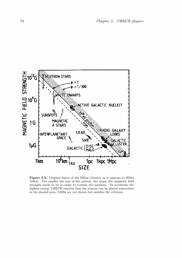
74 Chapter 5. UHECR physics
Figure 5.3. Original figure of the Hillas criterion as it appears in Hillas(1984). The smaller the size of the system, the larger the magnetic fieldstrength needs to be in order to contain the particles. To accelerate thehighest energy UHECR requires that the sources can be placed somewherein the shaded area. GRBs are not shown but satisfies the criterion.
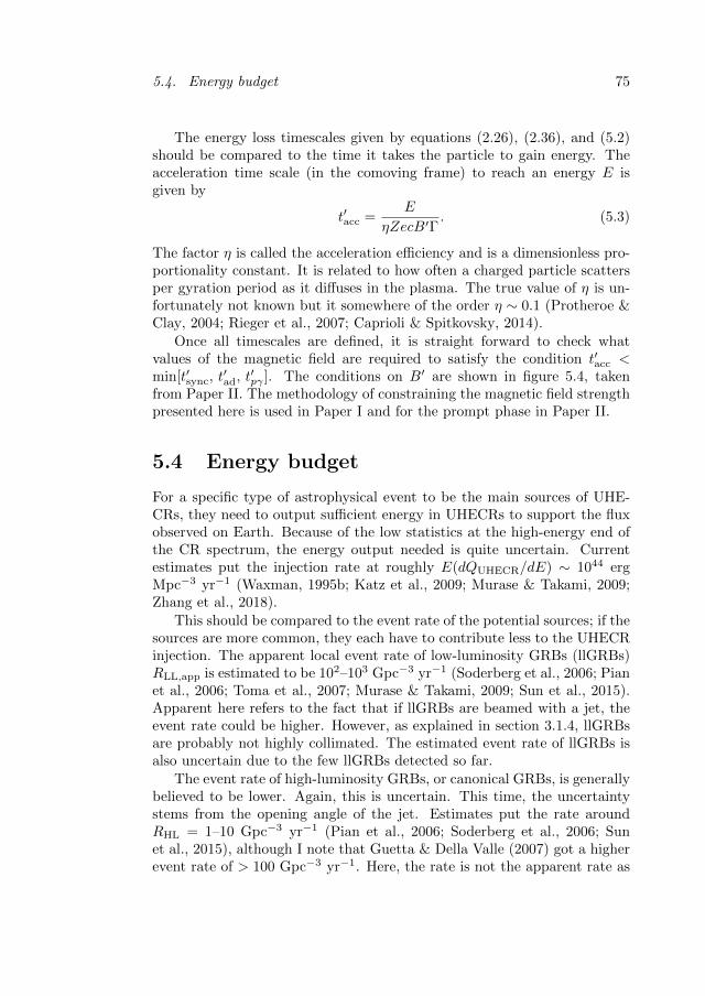
5.4. Energy budget 75
The energy loss timescales given by equations (2.26), (2.36), and (5.2)should be compared to the time it takes the particle to gain energy. Theacceleration time scale (in the comoving frame) to reach an energy E isgiven by
t′acc =E
ηZecB′Γ. (5.3)
The factor η is called the acceleration efficiency and is a dimensionless pro-portionality constant. It is related to how often a charged particle scattersper gyration period as it diffuses in the plasma. The true value of η is un-fortunately not known but it somewhere of the order η ∼ 0.1 (Protheroe &Clay, 2004; Rieger et al., 2007; Caprioli & Spitkovsky, 2014).
Once all timescales are defined, it is straight forward to check whatvalues of the magnetic field are required to satisfy the condition t′acc <min[t′sync, t
′ad, t
′pγ ]. The conditions on B′ are shown in figure 5.4, taken
from Paper II. The methodology of constraining the magnetic field strengthpresented here is used in Paper I and for the prompt phase in Paper II.
5.4 Energy budget
For a specific type of astrophysical event to be the main sources of UHE-CRs, they need to output sufficient energy in UHECRs to support the fluxobserved on Earth. Because of the low statistics at the high-energy end ofthe CR spectrum, the energy output needed is quite uncertain. Currentestimates put the injection rate at roughly E(dQUHECR/dE) ∼ 1044 ergMpc−3 yr−1 (Waxman, 1995b; Katz et al., 2009; Murase & Takami, 2009;Zhang et al., 2018).
This should be compared to the event rate of the potential sources; if thesources are more common, they each have to contribute less to the UHECRinjection. The apparent local event rate of low-luminosity GRBs (llGRBs)RLL,app is estimated to be 102–103 Gpc−3 yr−1 (Soderberg et al., 2006; Pianet al., 2006; Toma et al., 2007; Murase & Takami, 2009; Sun et al., 2015).Apparent here refers to the fact that if llGRBs are beamed with a jet, theevent rate could be higher. However, as explained in section 3.1.4, llGRBsare probably not highly collimated. The estimated event rate of llGRBs isalso uncertain due to the few llGRBs detected so far.
The event rate of high-luminosity GRBs, or canonical GRBs, is generallybelieved to be lower. Again, this is uncertain. This time, the uncertaintystems from the opening angle of the jet. Estimates put the rate aroundRHL = 1–10 Gpc−3 yr−1 (Pian et al., 2006; Soderberg et al., 2006; Sunet al., 2015), although I note that Guetta & Della Valle (2007) got a higherevent rate of > 100 Gpc−3 yr−1. Here, the rate is not the apparent rate as
76 Chapter 5. UHECR physics
Figure 5.4. Allowed parameter space for B′ as function of r and E for bulkLorentz factor Γ = 10. The color bar shows log(E/[eV]) for iron (Z = 26)and the vertical dashed line shows the photosphere (see section 3.3). Thetop x-axis shows the minimum variability time tv = r/2Γ2c. The dottedlines show the limits on B′ obtained from t′acc < t′sync, the dot-dashed linesshow the limits from t′acc < t′ad, and the solid lines show the limits fromt′acc < t′pγ , all for integer values of log(E/[eV]) as indicated in the plots.Figure adopted from Paper II.
5.4. Energy budget 77
high-luminosity GRBs are known to be relativistic and beaming has beenaccounted for.
Once UHECR energy injection rate and local rates of low- and high-luminosity GRBs are given, one can calculate how much energy on averageevery event needs to release in UHECR:
QUHECR/RLL,app = 1050QUHECR,44R−1LL,app,3 erg (5.4)
for llGRBs and
QUHECR/RHL = 1052QUHECR,44R−1HL,1 erg (5.5)
for high-luminosity GRBs. The energy budget requirement is used in PaperII.

78
Chapter 6
Summary of attachedpapers
In this chapter, I will briefly summarize the main arguments and results ofthe five attached papers.
6.1 Paper I
We investigate whether high- and/or low-luminosity GRBs can be majorsources of UHECRs. Paper I focuses on UHECR acceleration during theprompt phase. Two different scenarios are investigated with slightly dif-ferent methodology. In the first scenario, the observed prompt spectrumis dominated by synchrotron emission, while in the second scenario, theprompt radiation is dominated by photospheric emission (see sections 3.3and 3.4).
In the synchrotron emission scenario, we use known properties of ob-served GRB photon spectra to constrain the possibility of UHECR accel-eration. The νFν-peak energy, εpeak, in the spectrum occurs at roughly∼ 300 keV. In synchrotron models, the νFν-peak energy corresponds toεpeak = max[εm, εc], where εm and εc are the characteristic energies of pho-tons emitted by electrons with the characteristic Lorentz factor γ′m and γ′crespectively. Here, γ′m and γ′c are the injection and cooling Lorentz factoras described in Section 2.4). To account for acceleration up to the highestUHECR energies observed, GRBs need high magnetic fields strengths. Theelectrons subjected to these high magnetic fields quickly lose their energydue to synchrotron radiation, which decreases γ′c, and small values of γ′cresults in small values of εc. Indeed, for all the parameter space that would
79
80 Chapter 6. Summary of attached papers
allow for UHECR acceleration, εc εpeak, which implies that εm = εpeak
and that the electrons are very fast cooling. However, this is in tension withobservations that suggest observed GRB spectra to be at most marginallyfast cooling with γ′c . γ′m.
If the observed spectrum is photospheric, then we have to use a differ-ent argument. It is still true that the magnetic fields need to be high toaccount for UHECR acceleration and that the co-accelerated electrons emitsynchrotron radiation in this magnetic field. However, in this scenario theobserved spectrum is not from the accelerated electrons, thus we cannotassign εm = εpeak. Instead, we use the constraint that the emitted syn-chrotron radiation must be subdominant to the observed spectrum. If it isnot, then we can refer back to the previous argument of synchrotron dom-inated prompt emission. We found that the synchrotron radiation emittedby the co-accelerated electrons would be orders of magnitude higher thantypical GRB fluxes, specifically in optical frequencies. The high magneticfields needed for UHER acceleration results in very rapid energy losses forthe electrons, producing a high flux. This result was valid for both high andlow-luminosity GRBs.
Lastly, we investigated the parameter dependence of the results in PaperI. We found that if GRBs are responsible for UHECR acceleration, then it isnecessary that only a small fraction of the available electrons are accelerated.Furthermore, this small number fraction should receive a small portion ofthe energy in order to be consistent with observations. We suggested thathigh optical flux could be an indicative signature of successful UHECRacceleration.
6.2 Paper II
Following on Paper I, Paper II applied the same methodology to the spe-cific low-luminosity GRB 060218. An advantage of considering this specificGRB is that there exist very good data in several different energy bands.Therefore, where we in Paper I had to assume typical flux limits applicableto the whole GRB sample, in Paper II we could compare the predictions todirect measurements. Furthermore, Paper I extended on the work in PaperII by considering acceleration of UHECR during the afterglow phase as well.
For the prompt phase we used the same methodology as for the pho-tospheric models in Paper I. Indeed, that the produced flux from the co-accelerated electrons cannot be brighter than the observations is true re-gardless of the prompt emission model. The results for GRB 060218 weresimilar but much stronger to those presented for llGRBs in Paper I. Theresults were stronger because the optical measurement of GRB 060218 ismuch lower than the optical flux limit used for llGRBs in Paper I.
6.3. Paper III 81
For the afterglow phase we used a different method. The method for theafterglow was similar to that of the prompt as both compared the predictedemission from the co-accelerated electrons with observation to constrain thepossibility of UHECR acceleration. However, for the afterglow phase, weused the fact that the afterglow blast wave had to contain the required min-imum energy to supply the observed flux of UHECR at Earth, as describedin Section 5.4. This energy was much higher than previous estimates ofthe afterglow energy in GRB 060218. This forced us to consider a compos-ite model for the electron distribution, where a fraction ξa of the electronswere accelerated into a power-law while the rest (1−ξa) were thermal. Withthe thermal electrons included, the total energy of the blast wave could beconstrained.
We found that the thermal electrons radiate mostly in the radio band.Comparing the emission from the thermal electrons to the radio data at∼ 3 days, we found that the parameters necessary to be consistent withthe radio data are disfavored by particle-in-cell simulations. However, if theenergy of the blast wave was reduced, we found that the radio data could besatisfied with parameter values in line with predictions. We concluded thatthe afterglow phase of GRB 060218 likely did not have sufficient energyto be a major source of UHECRs. Lastly, we argued that because GRB060218 seemed comparable to other llGRBs in terms of prompt optical fluxand afterglow radio flux, these result might extend to the whole llGRBpopulation.
6.3 Paper III
In Paper III, we developed an approximation capable of simulating RMSs inGRBs at very low computational cost. The approximation builds upon thefact that the change that occur to the photon distribution as it traverses anRMS is very similar to thermal Comptonization on hot electrons. With thisrealization, we constructed the Kompaneets RMS approximation (KRA).The output of the KRA was tested against the simulation code radshock,which is a self-consistent radiation hydrodynamic code (Lundman et al.,2018). Using analytical arguments and empirical tests, we managed to relatethe free parameters of both models to one another, and found excellentagreement between the outputs of both models.
RMSs may play an important role in the prompt emission of GRBs.However, before our work in Paper III, no such model had been fitted todata due to the computational cost of simulating RMSs. However, withKomrad, which is the name of the simulation program implementing theKRA, we gained about four orders of magnitude in computational timecompared to the full scale radiation hydrodynamic simulations. With this
82 Chapter 6. Summary of attached papers
massive time reduction, we could simulate a large enough parameter spaceto be able to fit the model to data.
Implementing a minimal shock model, we simulated the photosphericspectrum expected after a subphotospheric collision had dissipated energythrough an RMS. With the Komrad spectra, we were able to perform a fitto a time resolved spectrum in GRB 150314A. This was the first time anRMS model had been fitted to GRB data. The fit allowed us to uncover thephysical properties of the RMS, such as the shock velocity and the upstreamtemperature.
6.4 Paper IV
Motivated by the work of Ghisellini et al. (2020), we considered observa-tional signatures of proton synchrotron models as the prompt emission inGRBs. Specifically, we considered the emission from BeHe pairs createdin the interaction between the protons and their self-generated synchrotronphoton field. We found that in the conditions expected in GRB jets, alarge parameter region allowed for significant cooling by BeHe pair creationwhile not allowing pion production, which implies that BeHe pair creationcan significantly alter the evolution of the system.
Neglecting pion creation, we found that there are two different regions ofinterest by comparing the proton cooling timescales of proton synchrotronemission and BeHe pair production. In the first region, proton synchrotronemission dominates with little effect from BeHe pair creation. This occurswhen the photon densities are sufficiently low, namely for low bulk Lorentzfactors, large emission radii, and low luminosities. In the second region,cooling by creation of BeHe pairs dominates over synchrotron cooling. Thishappens in the opposite regime of high photon density. In this case, theemission from the abundance of BeHe pairs dominates the spectrum in theobservable range of the Fermi detectors, creating a single soft power lawinconsistent with observations.
However, quite a large parameter range results in cooling timescales thatare comparable. In this intermediate region between the two extremes, sig-natures from both protons synchrotron emission and BeHe pair synchrotronemission can be visible in the observed spectrum. In this case, the spectrumis double peaked. Furthermore, the ratio of the two peaks is in the range∼ 102 − 104, largely independent on the parameters. Such a signature hasbeen seen in the spectrum of several GRBs, most noteworthy GRB 190114Cseen by the MAGIC telescope (see figure 3.6, MAGIC Collaboration et al.,2019; Chand et al., 2020).
6.5. Paper V 83
6.5 Paper V
Paper V is a continuation of the work conducted in Paper III. In PaperIII, we developed the KRA. We verified that the approximation was validby comparing it to full scale radiation hydrodynamic simulations and weperformed a fit to a GRB spectrum for the first time. In Paper V, we usedthe KRA to qualitatively assess the observational characteristics of RMS inGRB prompt spectra.
Relevant parameter ranges for the free parameters in the KRA werenot known a priori: without putting it into the context of a GRB jet, theparameters could take basically any value. To estimate the parameter valuesrelevant for the system at hand, we used an internal collision framework (seesection 3.2.3). Using this framework, we obtained the KRA parameters fromhigher order parameters such as the Lorentz factor of the outflow and theoptical depth of the collision. When the KRA parameters were obtained, wegenerated synthetic photospheric spectra using the simulation code Komrad.We folded the synthetic spectra through the Fermi response and then fittedit with a phenomenological cutoff power-law (CPL) function. The CPLfunction is commonly used in catalogues and this allowed us to comparethe fitted parameters obtained to catalogues of real observations. The CPLfunction has two parameters of interest, namely the low-energy power lawslope αcpl and the peak spectrum Epeak.
We found that the results are sensitive to the conditions at the base of thejet, specifically the radius at which the free fireball acceleration starts, r0.We tried two different scenarios for r0. In the first scenario, the accelerationstarts close to the central engine with r0 = 107 cm. In this case we foundthat the spectra were hard, with low-energy slope αcpl & −0.5. Such hardvalues of the power-law slope cannot explain the majority of observed GRBpulses, which have αcpl & −1. In the second scenario, we used r0 = 1010 cm.This large value of r0 was suggested quite early on and has also been foundaccurate in various hydrodynamical jet simulations (Thompson et al., 2007;Lazzati et al., 2009; Lopez-Camara et al., 2013; Gottlieb et al., 2018, 2019,2021). In this case, the distributions obtained for both αcpl and Epeak aresimilar to the catalogued distributions from observations (see figure 3.5).The spectra obtained contain an additional low-energy break in X-rays,similar to those observed in Ravasio et al. (2018, 2019) (see section 3.1.3).
Finally, we identified a quite large parameter region of what we call“optically shallow shocks”. Optically shallow shocks are RMSs that do nothave time to reach steady state before the dissipation ends. This means thatsignatures of the shocks formation may still be imprinted in the releasedspectrum. We showed that optically shallow shocks occur as deep as τ ∼55u2
u. Therefore, for mildly relativistic shocks with uu . 1, steady state
84 Chapter 6. Summary of attached papers
is not obtained until after ∼ 100 scatterings. However, for our sample inPaper V, the average value of uu is often larger and optically shallow shocksare less frequent.
Acknowledgments
I would like to thank my supervisor Felix Ryde, and my close collaboratorsDamien Begue and Christoffer Lundman for their continuous supervisionand support. A special thanks to Asaf Pe’er for his supervision during mytime at Bar-Ilan University. I also thank my friends and colleagues at theParticle and Astroparticle Physics department. Lastly, I thank my fianceeAngelica Alamaa, my family, and my friends for brightening the real life,outside of the office.
85

86
Bibliography
Aab A., et al., 2016, Physics Letters B, 762, 288
Aab A., et al., 2020, PRL, 125, 121106
Abbott B. P., et al., 2017a, PRL, 119, 161101
Abbott B. P., et al., 2017b, ApJL, 848, L12
Abraham J., et al., 2004, Nuclear Instruments and Methods in PhysicsResearch A, 523, 50
Abramowicz M. A., Novikov I. D., Paczynski B., 1991, ApJ, 369, 175
Acuner Z., Ryde F., Yu H.-F., 2019, MNRAS, 487, 5508
Acuner Z., Ryde F., Pe’er A., Mortlock D., Ahlgren B., 2020, ApJ, 893, 128
Ahlers M., Halzen F., 2018, Progress in Particle and Nuclear Physics, 102,73
Ahlgren B., Larsson J., Nymark T., Ryde F., Pe’er A., 2015, MNRAS, 454,L31
Axelsson M., et al., 2012, ApJL, 757, L31
Band D., et al., 1993, ApJ, 413, 281
Barat C., Lestrade J. P., Dezalay J. P., Hurley K., Sunyaev R., Terekhov O.,Kuznetsov A., 1998, in Meegan C. A., Preece R. D., Koshut T. M., eds,American Institute of Physics Conference Series Vol. 428, Gamma-RayBursts, 4th Hunstville Symposium. pp 278–283, doi:10.1063/1.55335
Bell A. R., 1978, MNRAS, 182, 147
Beloborodov A. M., 2010, MNRAS, 407, 1033
Beloborodov A. M., 2017, ApJ, 838, 125
87
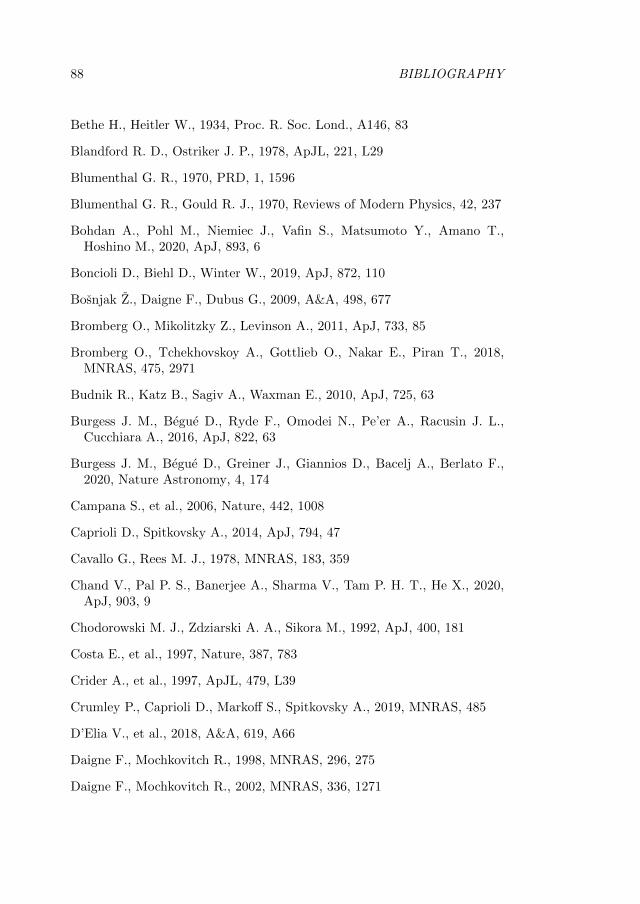
88 BIBLIOGRAPHY
Bethe H., Heitler W., 1934, Proc. R. Soc. Lond., A146, 83
Blandford R. D., Ostriker J. P., 1978, ApJL, 221, L29
Blumenthal G. R., 1970, PRD, 1, 1596
Blumenthal G. R., Gould R. J., 1970, Reviews of Modern Physics, 42, 237
Bohdan A., Pohl M., Niemiec J., Vafin S., Matsumoto Y., Amano T.,Hoshino M., 2020, ApJ, 893, 6
Boncioli D., Biehl D., Winter W., 2019, ApJ, 872, 110
Bosnjak Z., Daigne F., Dubus G., 2009, A&A, 498, 677
Bromberg O., Mikolitzky Z., Levinson A., 2011, ApJ, 733, 85
Bromberg O., Tchekhovskoy A., Gottlieb O., Nakar E., Piran T., 2018,MNRAS, 475, 2971
Budnik R., Katz B., Sagiv A., Waxman E., 2010, ApJ, 725, 63
Burgess J. M., Begue D., Ryde F., Omodei N., Pe’er A., Racusin J. L.,Cucchiara A., 2016, ApJ, 822, 63
Burgess J. M., Begue D., Greiner J., Giannios D., Bacelj A., Berlato F.,2020, Nature Astronomy, 4, 174
Campana S., et al., 2006, Nature, 442, 1008
Caprioli D., Spitkovsky A., 2014, ApJ, 794, 47
Cavallo G., Rees M. J., 1978, MNRAS, 183, 359
Chand V., Pal P. S., Banerjee A., Sharma V., Tam P. H. T., He X., 2020,ApJ, 903, 9
Chodorowski M. J., Zdziarski A. A., Sikora M., 1992, ApJ, 400, 181
Costa E., et al., 1997, Nature, 387, 783
Crider A., et al., 1997, ApJL, 479, L39
Crumley P., Caprioli D., Markoff S., Spitkovsky A., 2019, MNRAS, 485
D’Elia V., et al., 2018, A&A, 619, A66
Daigne F., Mochkovitch R., 1998, MNRAS, 296, 275
Daigne F., Mochkovitch R., 2002, MNRAS, 336, 1271
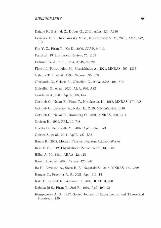
BIBLIOGRAPHY 89
Daigne F., Bosnjak Z., Dubus G., 2011, A&A, 526, A110
Derishev E. V., Kocharovsky V. V., Kocharovsky V. V., 2001, A&A, 372,1071
Fan Y.-Z., Piran T., Xu D., 2006, JCAP, 9, 013
Fermi E., 1949, Physical Review, 75, 1169
Fishman G. J., et al., 1994, ApJS, 92, 229
Florou I., Petropoulou M., Mastichiadis A., 2021, MNRAS, 505, 1367
Galama T. J., et al., 1998, Nature, 395, 670
Ghirlanda G., Celotti A., Ghisellini G., 2003, A&A, 406, 879
Ghisellini G., et al., 2020, A&A, 636, A82
Goodman J., 1986, ApJL, 308, L47
Gottlieb O., Nakar E., Piran T., Hotokezaka K., 2018, MNRAS, 479, 588
Gottlieb O., Levinson A., Nakar E., 2019, MNRAS, 488, 1416
Gottlieb O., Nakar E., Bromberg O., 2021, MNRAS, 500, 3511
Greisen K., 1966, PRL, 16, 748
Guetta D., Della Valle M., 2007, ApJL, 657, L73
Guiriec S., et al., 2011, ApJL, 727, L33
Harris R., 2008, Modern Physics. Pearson/Addison-Wesley
Hess V. F., 1912, Physikalische Zeitschrschift, 13, 1084
Hillas A. M., 1984, ARAA, 22, 425
Hjorth J., et al., 2003, Nature, 423, 847
Ito H., Levinson A., Stern B. E., Nagataki S., 2018, MNRAS, 474, 2828
Kangas T., Fruchter A. S., 2021, ApJ, 911, 14
Katz B., Budnik R., Waxman E., 2009, JCAP, 3, 020
Kobayashi S., Piran T., Sari R., 1997, ApJ, 490, 92
Kompaneets A. S., 1957, Soviet Journal of Experimental and TheoreticalPhysics, 4, 730
90 BIBLIOGRAPHY
Kouveliotou C., Meegan C. A., Fishman G. J., Bhat N. P., Briggs M. S.,Koshut T. M., Paciesas W. S., Pendleton G. N., 1993, ApJL, 413, L101
Lazzati D., Morsony B. J., Begelman M. C., 2009, ApJL, 700, L47
Levinson A., Bromberg O., 2008, PRL, 100, 131101
Levinson A., Nakar E., 2020, PhysRep , 866, 1
Lopez-Camara D., Morsony B. J., Begelman M. C., Lazzati D., 2013, ApJ,767, 19
Lundman C., Beloborodov A. M., 2019, ApJ, 879, 83
Lundman C., Beloborodov A. M., 2021, ApJL, 907, L13
Lundman C., Pe’er A., Ryde F., 2013, MNRAS, 428, 2430
Lundman C., Beloborodov A. M., Vurm I., 2018, ApJ, 858, 7
MAGIC Collaboration et al., 2019, Nature, 575, 455
Mastichiadis A., Protheroe R. J., Kirk J. G., 2005, A&A, 433, 765
Mei A., et al., 2022, arXiv e-prints, p. arXiv:2203.04971
Meszaros P., 2006, Reports on Progress in Physics, 69, 2259
Mochkovitch R., Hernanz M., Isern J., Martin X., 1993, Nature, 361, 236
Mucke A., Rachen J. P., Engel R., Protheroe R. J., Stanev T., 1999, PASA,16, 160
Murase K., Takami H., 2009, ApJL, 690, L14
NASA, ESA, J. Hester and A. Loll 2004, Crab Nebula, http://
hubblesite.org/gallery/album/entire_collection/pr2004032d/
NASA Science Official 1995, Bow shock in orion nebula as seen by Hubble,https://www.nasa.gov/images/content/52706main_hstorion_lg.
jpg
Nakar E., Sari R., 2012, ApJ, 747, 88
Nakar E., Ando S., Sari R., 2009, ApJ, 703, 675
Oganesyan G., Nava L., Ghirlanda G., Melandri A., Celotti A., 2019, A&A,628, A59
Paczynski B., 1986, ApJL, 308, L43
BIBLIOGRAPHY 91
Pe’er A., 2008, ApJ, 682, 463
Pe’er A., 2015, Advances in Astronomy, 2015, 907321
Pe’er A., Meszaros P., Rees M. J., 2006, ApJ, 642, 995
Pian E., et al., 2006, Nature, 442, 1011
Pinfold J., Atlas Collaboration 2017, in European Physical Journal Web ofConferences. p. 10001, doi:10.1051/epjconf/201714510001
Piran T., Shemi A., Narayan R., 1993, MNRAS, 263, 861
Preece R. D., Briggs M. S., Mallozzi R. S., Pendleton G. N., Paciesas W. S.,Band D. L., 1998, ApJL, 506, L23
Protheroe R. J., Clay R. W., 2004, PASA, 21, 1
Ravasio M. E., Oganesyan G., Ghirlanda G., Nava L., Ghisellini G., PescalliA., Celotti A., 2018, A&A, 613, A16
Ravasio M. E., Ghirlanda G., Nava L., Ghisellini G., 2019, A&A, 625, A60
Rees M. J., Meszaros P., 1992, MNRAS, 258, 41P
Rees M. J., Meszaros P., 1994, ApJL, 430, L93
Rees M. J., Meszaros P., 2005, ApJ, 628, 847
Rieger F. M., Bosch-Ramon V., Duffy P., 2007, ApSS , 309, 119
Ruderman M., 1975, in Bergman P. G., Fenyves E. J., Motz L., eds, SeventhTexas Symposium on Relativistic Astrophysics Vol. 262, Seventh TexasSymposium on Relativistic Astrophysics. pp 164–180, doi:10.1111/j.1749-6632.1975.tb31430.x
Rybicki G. B., Lightman A. P., 1979, Radiative processes in astrophysics.John Wiley & Sons, Inc
Ryde F., 2004, ApJ, 614, 827
Ryde F., 2005, ApJL, 625, L95
Ryde F., et al., 2010, ApJL, 709, L172
Ryde F., et al., 2011, MNRAS, 415, 3693
Ryde F., Lundman C., Acuner Z., 2017, MNRAS, 472, 1897
Samuelsson F., 2020, Multi-messenger emission from gamma-ray bursts
92 BIBLIOGRAPHY
Sari R., Piran T., Narayan R., 1998, ApJL, 497, L17
Sazonov S. Y., Lutovinov A. A., Sunyaev R. A., 2004, Nature, 430, 646
Schilling G., 2002, Flash! The hunt for the biggest explosions in the uni-verse.. Cambridge University Press
Schmidt W. K. H., 1978, Nature, 271, 525
Sironi L., Spitkovsky A., 2011, ApJ, 726, 75
Soderberg A. M., et al., 2006, Nature, 442, 1014
Starling R. L. C., et al., 2011, MNRAS, 411, 2792
Sun H., Zhang B., Li Z., 2015, ApJ, 812, 33
The Pierre Auger Collaboration et al., 2015, arXiv e-prints, p.arXiv:1509.03732
Thompson C., Meszaros P., Rees M. J., 2007, ApJ, 666, 1012
Toma K., Ioka K., Sakamoto T., Nakamura T., 2007, ApJ, 659, 1420
Treumann R. A., Jaroschek C. H., 2008, arXiv e-prints, p. arXiv:0806.4046
Vianello G., Gill R., Granot J., Omodei N., Cohen-Tanugi J., Longo F.,2018, ApJ, 864, 163
Waxman E., 1995a, Physical Review Letters, 75, 386
Waxman E., 1995b, ApJL, 452, L1
Waxman E., Meszaros P., Campana S., 2007, ApJ, 667, 351
Weaver T. A., 1976, ApJS, 32, 233
Wulf T., 1910, Physikalische Zeitschrschift, 11, 811
Yu H.-F., et al., 2016, A&A, 588, A135
Yu H.-F., Dereli-Begue H., Ryde F., 2019, ApJ, 886, 20
Zatsepin G. T., Kuz’min V. A., 1966, Soviet Journal of Experimental andTheoretical Physics Letters, 4, 78
Zhang B. T., Murase K., 2019, PRD, 100, 103004
Zhang B. T., Murase K., Kimura S. S., Horiuchi S., Meszaros P., 2018,PRD, 97, 083010
Related Documents