Cosmic Ray Observatory Project Fr Michael LieblAGU Conference Mount Michael Benedictine High SchoolDecember 6, 2005 Elkhorn Ne 68022.

Cosmic Ray Observatory ProjectFr Michael Liebl AGU Conference

Mount Michael Benedictine High School December 6, 2005

Elkhorn Ne 68022

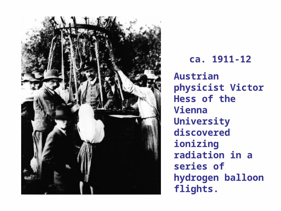
ca. 1911-12

Austrian physicist Victor Hess of the Vienna University discovered ionizing radiation in a series of hydrogen balloon flights.

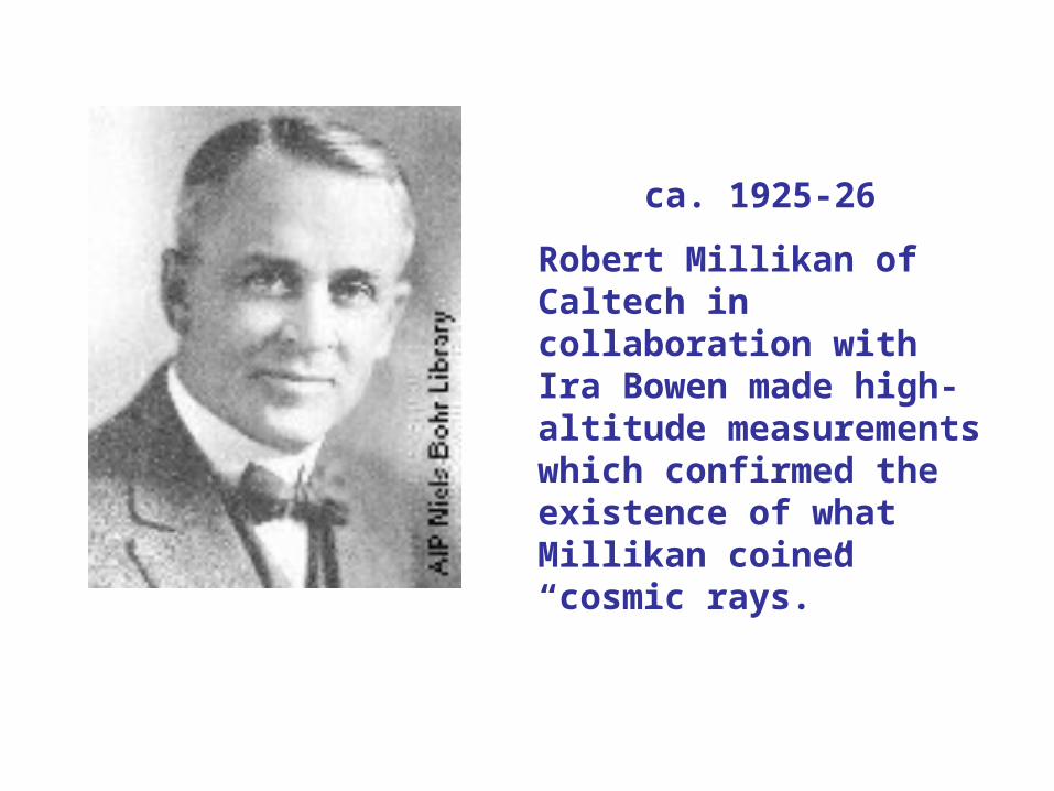
ca. 1925-26

Robert Millikan of Caltech in collaboration with Ira Bowen made high-altitude measurements which confirmed the existence of what Millikan coined “cosmic rays.”

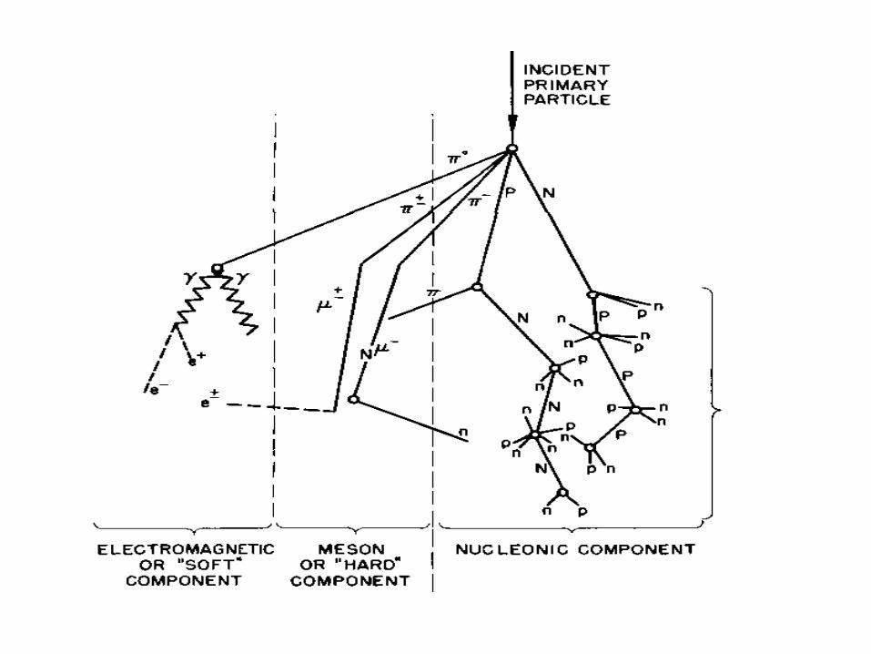
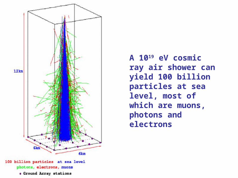
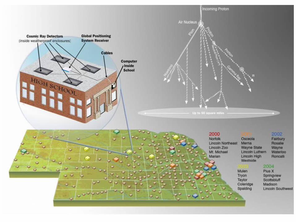
A 1019 eV cosmic ray air shower can yield 100 billion particles at sea level, most of which are muons, photons and electrons

Dr. Greg Snow

Dr. Dan Claes

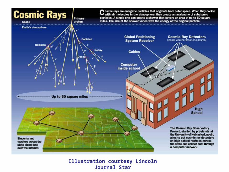
Illustration courtesy Lincoln Journal Star

PROJECT GOALS

Educational:

• Train teams of high school teachers and students to study cosmic rays

Scientific:

• Build a statewide network of cosmic ray detectors

• Search for the sources of ultra-high energy cosmic rays

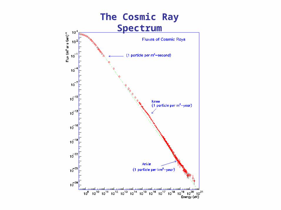
The Cosmic Ray Spectrum

Chicago Air Shower Array (CASA)

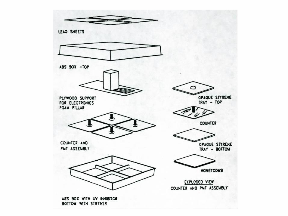
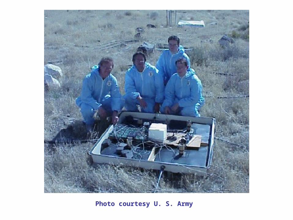
Photo courtesy U. S. Army

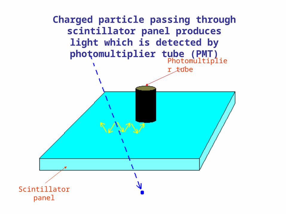
Charged particle passing through scintillator panel produces light which is detected by photomultiplier tube (PMT)

Photomultiplier tube

Scintillator panel

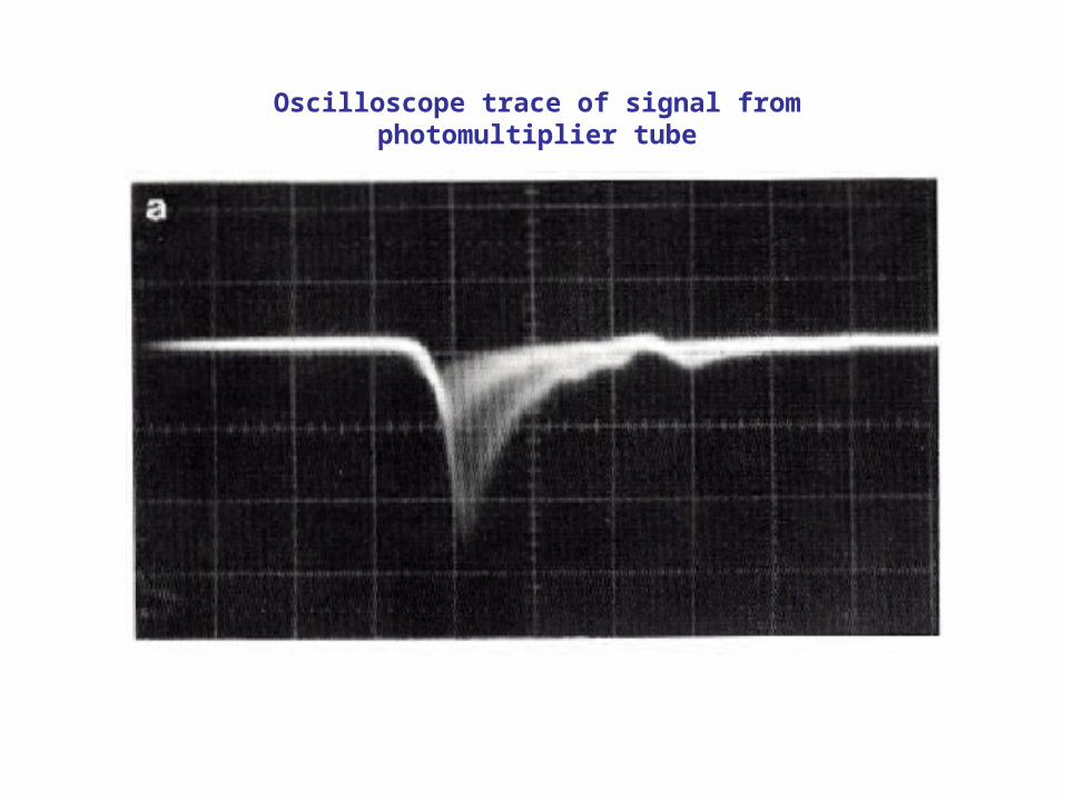
Oscilloscope trace of signal from photomultiplier tube

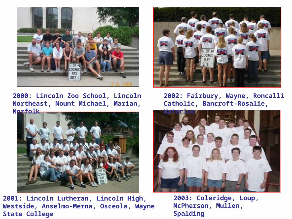
2000: Lincoln Zoo School, Lincoln Northeast, Mount Michael, Marian, Norfolk

2002: Fairbury, Wayne, Roncalli Catholic, Bancroft-Rosalie, Waterloo

2001: Lincoln Lutheran, Lincoln High, Westside, Anselmo-Merna, Osceola, Wayne State College

2003: Coleridge, Loup, McPherson, Mullen, Spalding

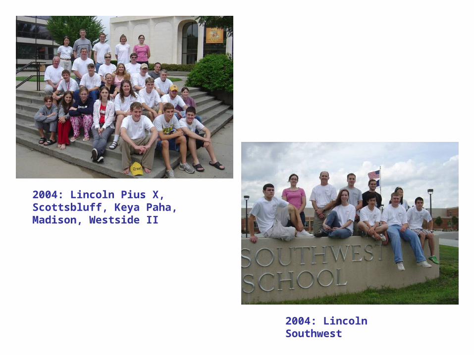
2004: Lincoln Pius X, Scottsbluff, Keya Paha, Madison, Westside II

2004: Lincoln Southwest

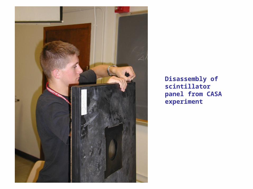
Disassembly of scintillator panel from CASA experiment

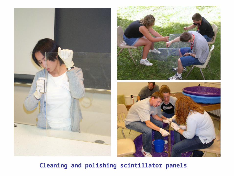
Cleaning and polishing scintillator panels

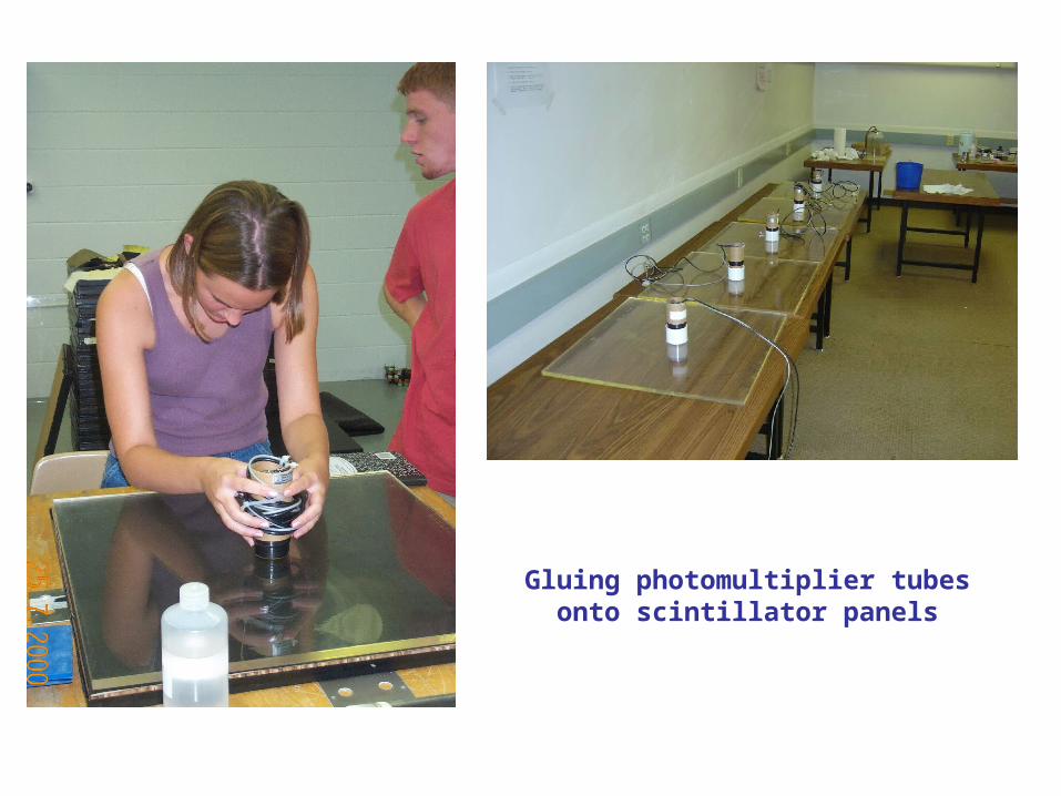
Gluing photomultiplier tubes onto scintillator panels

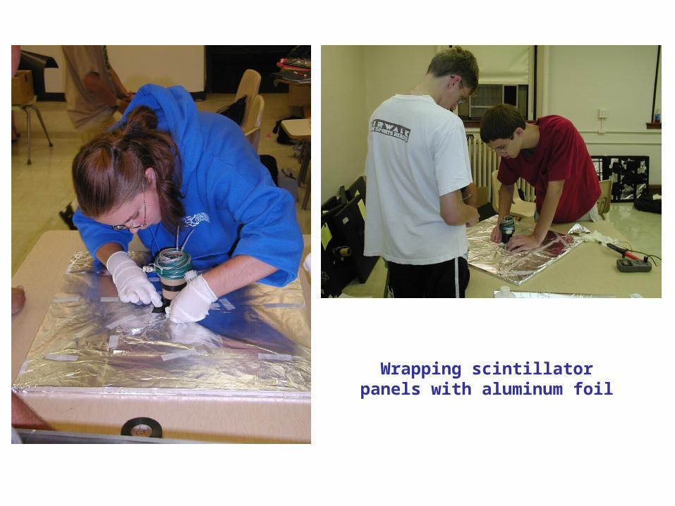
Wrapping scintillator panels with aluminum foil

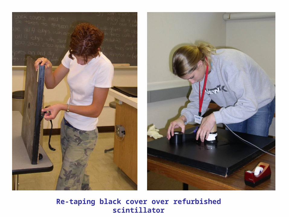
Re-taping black cover over refurbished scintillator

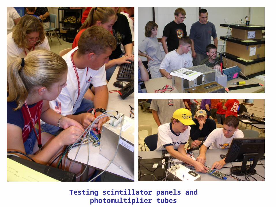
Testing scintillator panels and photomultiplier tubes

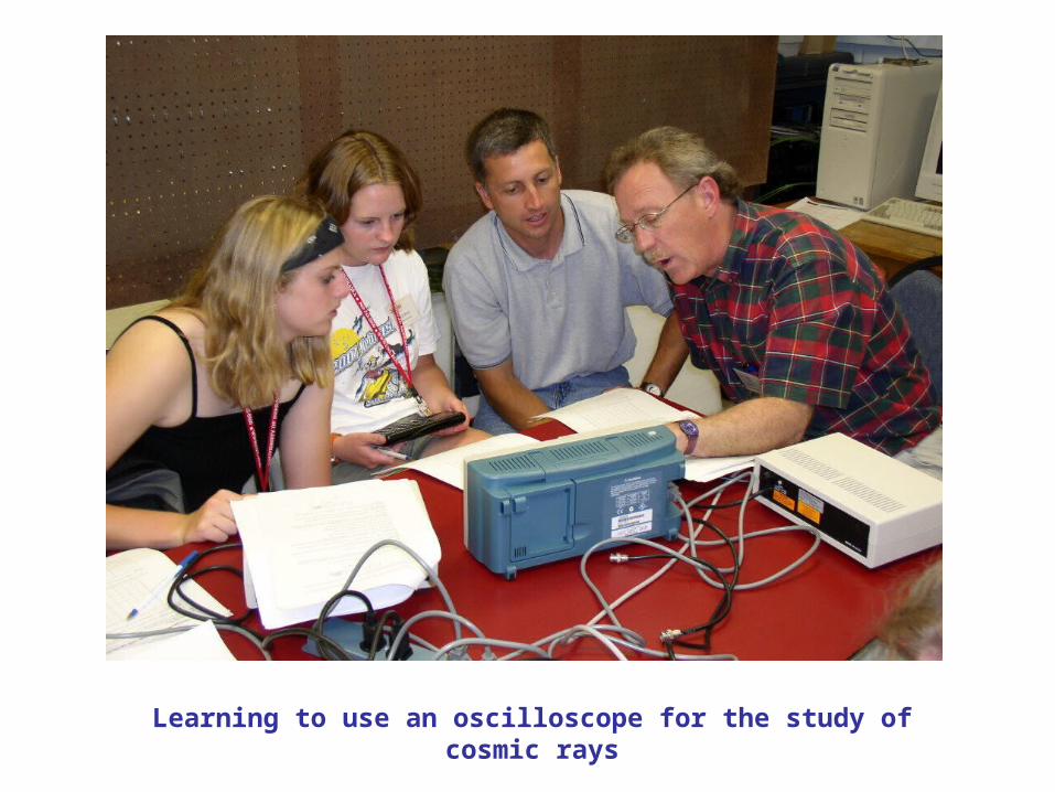
Learning to use an oscilloscope for the study of cosmic rays

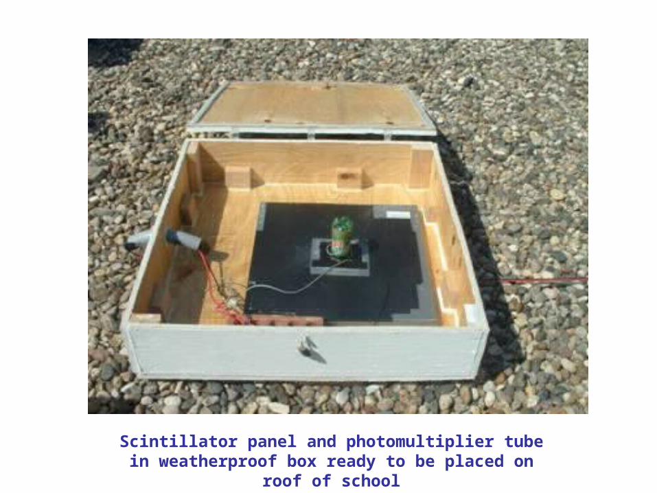
Scintillator panel and photomultiplier tube in weatherproof box ready to be placed on roof of school

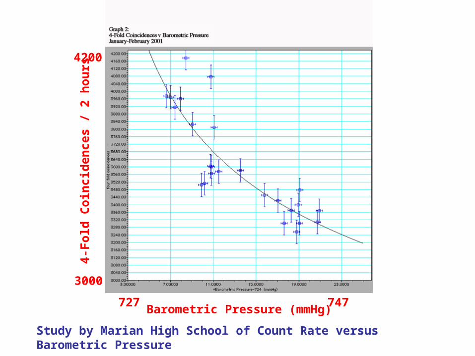
Barometric Pressure (mmHg)727 747

4-F

old

Coi

ncid

ence

s / 2

hou

rs

3000

4200

Study by Marian High School of Count Rate versus Barometric Pressure

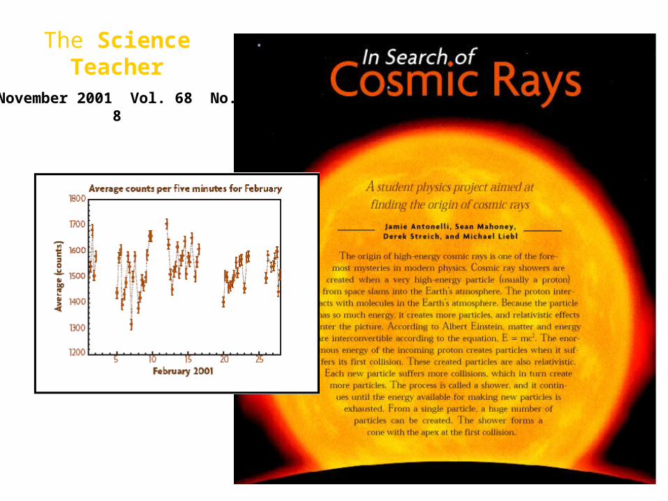
The Science TeacherNovember 2001 Vol. 68 No. 8

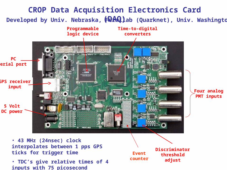
5 VoltDC power

PCserial port

Four analogPMT inputs

Discriminatorthreshold

adjust

GPS receiverinput

Programmablelogic device

Time-to-digitalconverters

Developed by Univ. Nebraska, Fermilab (Quarknet), Univ. Washington

CROP Data Acquisition Electronics Card (DAQ)

Event counter

• 43 MHz (24nsec) clock interpolates between 1 pps GPS ticks for trigger time

• TDC’s give relative times of 4 inputs with 75 picosecond resolution

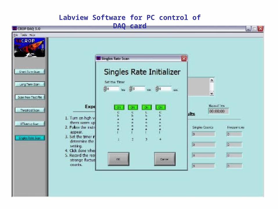
Labview Software for PC control of DAQ card

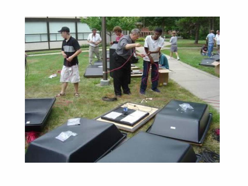
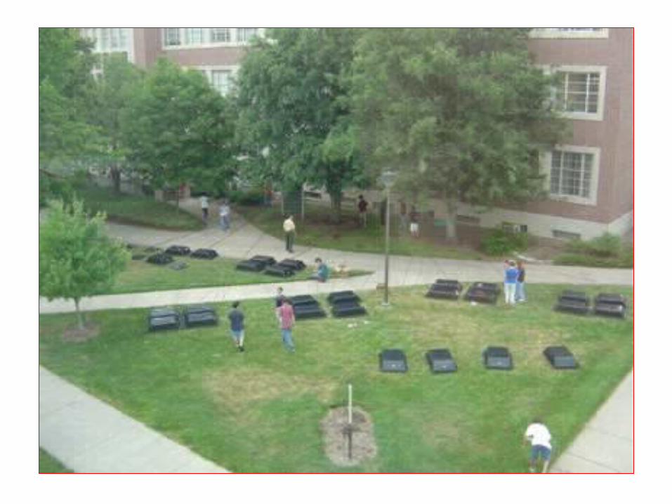
Summer 2005 Workshop

• Bring participating schools to Lincoln campus

• Refresh skills on use of equipment

• Replace damaged or non-functioning equipment

• Proof of principle experiment

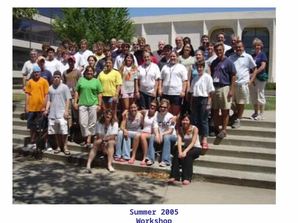
Summer 2005 Workshop

Challenges

• Distances between schools are large

• Replacement or repair of equipment

• Rural schools sometimes have no physics teacher

• Rural schools may have physics teachers teaching out of discipline

• Replacing trained students

• Support of local school administration

• Maintaining enthusiasm over prolonged time span

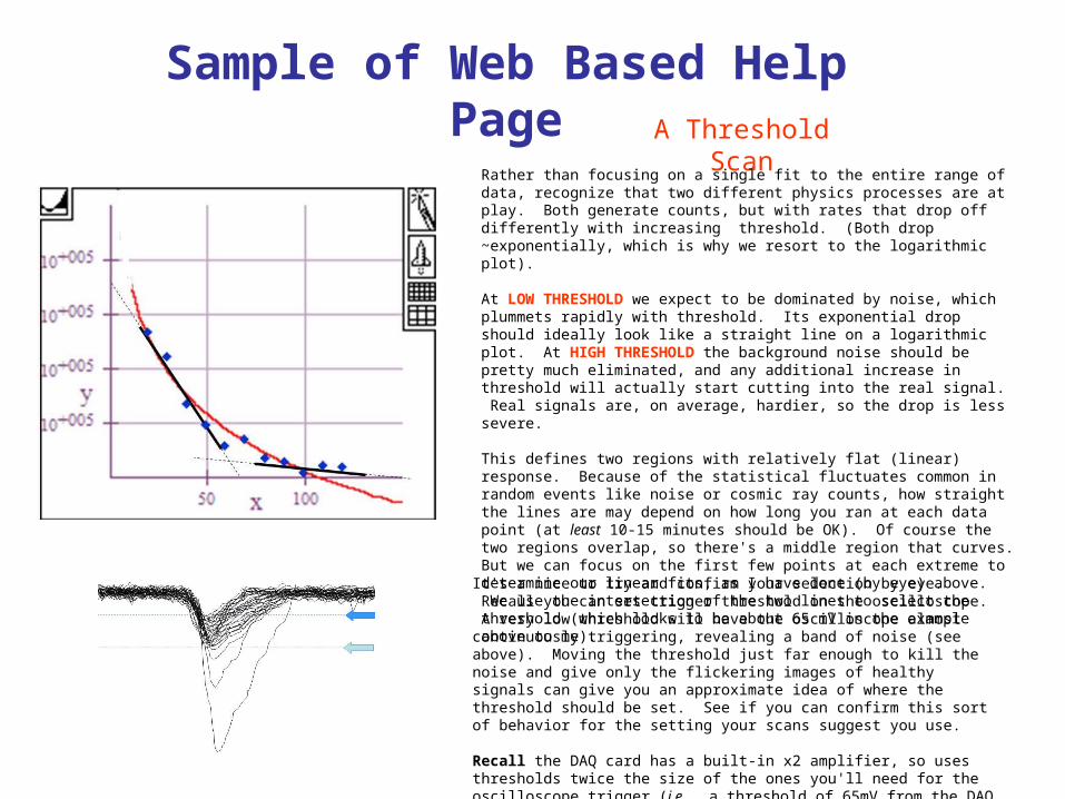
A Threshold Scan

Rather than focusing on a single fit to the entire range of data, recognize that two different physics processes are at play.  Both generate counts, but with rates that drop off differently with increasing  threshold.  (Both drop ~exponentially, which is why we resort to the logarithmic plot).

At LOW THRESHOLD we expect to be dominated by noise, which plummets rapidly with threshold.  Its exponential drop should ideally look like a straight line on a logarithmic plot.  At HIGH THRESHOLD the background noise should be pretty much eliminated, and any additional increase in threshold will actually start cutting into the real signal.  Real signals are, on average, hardier, so the drop is less severe.

This defines two regions with relatively flat (linear) response.  Because of the statistical fluctuates common in random events like noise or cosmic ray counts, how straight the lines are may depend on how long you ran at each data point (at least 10-15 minutes should be OK).  Of course the two regions overlap, so there's a middle region that curves. But we can focus on the first few points at each extreme to determine our linear fits, as I have done (by eye) above.  We use the intersection of the two lines to select the threshold (which looks to be about 65 mV in the example above to me).

It's a nice to try and confirm your selection by eye.  Recall you can set trigger threshold on the oscilloscope.  A very low threshold will have the oscilloscope almost continuously triggering, revealing a band of noise (see above).  Moving the threshold just far enough to kill the noise and give only the flickering images of healthy signals can give you an approximate idea of where the threshold should be set.  See if you can confirm this sort of behavior for the setting your scans suggest you use.  

Recall the DAQ card has a built-in x2 amplifier, so uses thresholds twice the size of the ones you'll need for the oscilloscope trigger (i.e., a threshold of 65mV from the DAQ card scan corresponds to a 32mV trigger threshold on the oscilloscope).

Sample of Web Based Help Page

FUTURE

• Duplicate 2005 workshop experiment with detectors on school rooftops

• Begin integration of results from dispersed detectors

• Bring more schools on line

• Secure additional funding for the future of CROP

• Coordinate activities with other high school cosmic ray projects

CROP Website

http://crop.unl.edu