Cosmic Ray Exposure Ages Of Stony Meteorites: Space Erosion Or Yarkovsky? · 2014-10-30 · Of Stony Meteorites: Space Erosion Or Yarkovsky? by David Parry Rubincam ... In that case

Rubincam 2/12/14 1

Cosmic Ray Exposure Ages

Of Stony Meteorites:

Space Erosion

Or Yarkovsky?

by

David Parry Rubincam

Code 698

Planetary Geodynamics Laboratory

Solar System Exploration Division

NASA Goddard Space Flight Center

Building 34, Room S280

Greenbelt, MD 20771

voice: 301-614-6464

fax: 301-614-6522

email: [email protected]

https://ntrs.nasa.gov/search.jsp?R=20140010049 2018-07-11T08:08:41+00:00Z

Rubincam 2/12/14 2

Abstract

Space erosion from dust impacts may set upper limits on the cosmic ray exposure

(CRE) ages of stony meteorites. A meteoroid orbiting within the asteroid belt is

bombarded by both cosmic rays and interplanetary dust particles. Galactic cosmic rays

penetrate only the first few meters of the meteoroid; deeper regions are shielded. The dust

particle impacts create tiny craters on the meteoroid’s surface, wearing it away by space

erosion (abrasion) at a particular rate. Hence a particular point inside a meteoroid

accumulates cosmic ray products only until that point wears away, limiting CRE ages.

The results would apply to other regolith-free surfaces in the solar system as well, so that

abrasion may set upper CRE age limits which depend on the dusty environment.

Calculations based on N. Divine’s dust populations and on micrometeoroid cratering

indicate that stony meteoroids in circular ecliptic orbits at 2 AU will record 21Ne CRE

ages of ~176 × 106 years if dust masses are in the range 10-21 – 10-3 kg. This is in broad

agreement with the maximum observed CRE ages of ~100 × 106 years for stones. High

erosion rates in the inner solar system may limit the CRE ages of Near-Earth Asteroids

(NEAs) to ~120 × 106 years. If abrasion should prove to be ~6 times quicker than found

here, then space erosion may be responsible for many of the measured CRE ages of main

belt stony meteorites. In that case the CRE ages may not measure the drift time to the

resonances due to the Yarkovsky effects as in the standard scenario, and that for some

reason Yarkovsky is ineffective.

Rubincam 2/12/14 3

1. Introduction

The observed cosmic ray exposure (CRE) ages are typically ~1-100 × 106 years

for stony meteorites, while iron meteorites have CRE ages on the order of ~600 × 106

years (e.g., McSween, 1999; Norton, 1994; Wood, 1968; Wieler and Graf, 2001). The

usual explanation for the CRE ages of meteorites is catastrophic collision plus drift time

plus resonance. In this scenario, a catastrophic collision between bodies in the asteroid

belt creates fragments. Each fragment becomes a meteoroid. What are now fragments

were mostly material buried so deeply in the parent bodies that they were shielded from

galactic cosmic rays. The cosmic ray “clock” thus starts “ticking” once the fragments are

exposed to the rays (e.g., Greenberg and Nolan, 1989).

The exposure continues while a meteoroid drifts to a resonance. The main

mechanism for delivering meteoroids to the resonances is currently believed to be the

Yarkovsky effects (e.g., Öpik, 1951; Peterson, 1976; Rubincam, 1987, 1995; Afonso et

al., 1995; Bottke et al., 2000, 2002; Farinella and Vokrouhlicky, 1999). Irons drift slower

than stones because their higher density and higher thermal conductivity lessen the

Yarkovsky effects compared to stones, explaining their longer CRE ages.

In the Yarkovsky scenario, the drift time would mainly control a meteoroid’s

CRE age, since once it reaches a resonance, the meteoroid’s orbital eccentricity is rapidly

pumped up until its orbit crosses that of the Earth (Wisdom, 1983). The pumping

timescale is only ~ a few 106 years (Gladman et al., 1997); so this part of the delivery

process does not contribute much to the CRE age. Thereafter the meteoroid hits the Earth,

to be picked up as a meteorite.

Rubincam 2/12/14 4

Two issues regarding meteoroid CRE ages are investigated here. The first issue is

how space erosion by abrasion may at least place upper limits on stony meteorite CRE

ages. The basic idea is illustrated in Fig. 1. Impacts from interplanetary dust excavate

craters on a meteoroid, causing abrasion. Hence a meteoroid will slowly erode away over

time.

However long that process takes sets an upper limit on the meteoroid’s CRE age.

Clearly no point inside the meteoroid can accumulate cosmic ray products once that point

becomes the surface and erodes away. The first issue thus becomes: do the erosion upper

limits do any violence to the measured CRE ages? If the erosion upper limits tended to be

much shorter than the measured CRE ages, then there would be a problem. However, it is

found that the erosion CRE ages are > ~176 ×106 y for the assumed model for stony

meteoroids originating in the main belt. This is in broad agreement with the measured

CRE ages of < ~100 ×106 y and allows the Yarkovsky drift timescale.

The second issue is whether space erosion may not just set maximum ages, but

whether a better model might be reasonably expected to increase the erosion rate enough

to lower the CRE ages into the observed range of many meteorites. If so, then CRE age

may be decoupled from drift time. Stony meteoroids, for instance, could theoretically

drift for very long periods of time before reaching a resonance, and still have CRE ages

of (say) only ~30 × 106 y. Certainly meteoroids can drift for extremely long stretches of

time, because the iron meteoroids have characteristic CRE ages of ~600 × 106 years. This

leads to the provocative question: do CRE ages measure Yarkovsky drift times of stones

at all? Perhaps Yarkovsky is weakened or inoperative for some reason and something

slower causes the drift but still gives the observed CRE ages, thanks to space erosion.

Rubincam 2/12/14 5

On this second issue one can make arguments both for and against increasing the

erosion rate found here (see section 6). Further investigation is indicated to see whether

space erosion puts the Yarkovsky interpretation in jeopardy.

The present paper computes the rate of space erosion for stony meteoroids from

dust impacts. Divine’s (1993) interplanetary dust populations provide the impactors. Of

his five distinct populations, only the core and asteroidal populations are used here. His

eccentric, inclined, and halo populations make negligible contributions to abrasion and

are ignored. Divine considers dust particles with masses in the range 10-21 kg - 10-3 kg;

these limits are adopted here. The dust particles in his asteroidal population have typical

masses of ~10-6 kg, corresponding to particle diameters of ~1 mm = 10-3 m. Some of

Divine’s (1993) velocity equations are derived in the Appendix as an aid to following his

development.

The amount of mass excavated with each dust particle impact on a stony

meteoroid is based on the work of Gault et al. (1972). The mass lost from the meteoroid

by making these microcraters is typically many times the mass of the impacting particles.

Only the CRE ages derived from neon concentrations are examined here. The

21Ne production rates are based on Eugster et al (2006).

In the following, the impacting particles are termed “dust”, even though this

includes particles up to 1 g = 0.001 kg, which is about the mass of the American dime

coin (en.wiki.org/wiki/Dime_(United_States_coin)), the smallest coin of United States

currency. The term “meteoroid” is reserved for the object hit by the dust.

Space erosion is an old topic (Whipple and Fireman, 1959; Fisher, 1961;

Whipple, 1962; Schaeffer, 1981; Hughes, 1982; Wieler and Graf, 2001, p. 227, Welten et

Rubincam 2/12/14 6

al., 2001). The present paper focuses on space erosion by abrasion, and devotes only a

few words to spallation.

Divine’s (1993) elegant paper provides the conceptual framework for the present

investigation; it is a fitting capstone to his career (Nunes, 1997). The mathematical

treatment which follows differs only slightly from Divine’s. Readers uninterested in the

derivations can skip to Section 4.

2. Dust particle density

This section computes the number density of dust particles for the asteroidal and

core populations. The result agrees with Divine (1993), giving confidence in the results

that follow. The abrasion rate will be computed in the succeeding sections.

A dust particle’s Cartesian position is given by

r ˆ r = xˆ x + yˆ y + z ˆ z , (1)

where r is its distance from the Sun, ˆ r is the unit position vector, and ˆ x , ˆ y , and ˆ z are the

unit vectors along the x, y, and z axes, respectively, where the z-axis is normal to the

ecliptic. The dust particle is assumed to orbit the Sun in an ellipse, with the Keplerian

orbital elements being (a, e, I, Ω, ω, M), where a is the semimajor axis, e is the orbital

eccentricity, I is the orbital inclination to the ecliptic, and Ω is the nodal position. The

other two Keplerian elements, argument of perihelion ω and mean anomaly M, will not

be needed here. See Fig. 2 for the geometry of the orbit. Two auxiliary variables which

Rubincam 2/12/14 7

are used below are the perihelion distance r1 = a(1 − e) and the ecliptic latitude λ, where

sin λ = z/r. The unit vector ˆ n normal to the dust particle’s orbital plane is given by

ˆ n = (sin I sin Ω)ˆ x - (sin I cos Ω) ˆ y +(cos I)ˆ z , (2)

The notation above follows that of Divine (1993), apart from the substitution of I for his i

and ( ˆ x , ˆ y , ˆ z ) for his (u x ,u y , u z ).

The number density ND of dust particles in units of number per cubic meter is

given by:

ND =H D

ππN1r1

r (r − r1)1/2 dr10

r

∫

• pe

[−(r − r1) + (r + r1)e]1/ 2r −r1

r +r1

1

∫ de

• pI sin I

[(cos2 λλ − cos2 I ]1/2λ

π − λ

∫ dI . (3)

This can be written more compactly as

ND =H D

ππw(r1,e, I )dr1dedI∫∫∫ (4)

to save space, where

Rubincam 2/12/14 8

w(r1,e, I ) =N1r1

r (r − r1)1/2

pe

[−(r − r1)+ (r + r1)e]1/2

pI sin I

[cos2 λ − cos2 I ]1/2 (5)

(Divine, 1993). In the above HD is a cumulative number distribution

H D = H mm1

∞

∫ dmD , (6)

defined such that HD = 1 for m1 = 1 g = 10-3 kg; Hm is a differential number distribution

(Divine, 1993, p. 17,030).

In (3) pI is a distribution which depends only on inclination I and pe is a

distribution which depends only on eccentricity e. Both the core and asteroidal

populations have the same pI and pe. They follow the normalizations

pI0

ππ

∫ dI =1 (7)

pe0

1

∫ de =1 . (8)

As Matney and Kessler (1996) point out, though pe > 0 and pI > 0, they are not the

“textbook” probability distributions; so that pede, for example, is not the number of

objects between e and e + de. But as they also point out, Divine’s pI and pe are internally

consistent, and so will be used here. They are shown as the solid lines in Fig.s 3 and 4.

Rubincam 2/12/14 9

The integrals in (3) have to be evaluated. The first step in doing so is to express pI

and pe in functions different from the straight lines in Fig.s 3 and 4, but still hew closely

to their values. The new functions make the integrations over I and e in (3) more

convenient.

The pI distribution is the most easily dealt with. Divine (1993) writes it as a

piecewise function of the form c + bI. Here pI will instead be written piecewise in the

form of c + b cos I. This allows integrals of the form

cosn I sin I

[(cos2 λ − cos2 I]1/ 2λ

π − λ

∫ dI (9)

to be analytically evaluated by switching to the variable cos I. The resulting expressions

can be found from tables, such as given by Selby (1974, pp. 429). Table 1 gives the

constants used for pI; they are chosen so that the pI used here closely resembles Divine’s

pI, and obeys the normalization (7). Figure 3 compares the two functions. The agreement

is good.

Divine similarly writes pe as a piecewise function of the form c + be, but here it

will be written as a continuous polynomial function of e on the interval [0,1]. The

technique is as follows. First, the square root of Divine’s piecewise function is written as

a sum of Zernicke polynomials

pe1/ 2 = gi

i = 0

J / 2

∑ Zi(e) (10)

Rubincam 2/12/14 10

where Zi(e) is the unnormalized Zernicke polynomial of order i and is summed to the

finite value J/2. The Zernicke polynomials are orthogonal on [0,1] and are related to the

Legendre polynomials (e.g., Beckmann 1973, pp. 150-156). The Zernicke polynomials

are given by the equation

Zi (e) =(−1)i + k( i + k)!

(i − k)!(k!)2k = 0

i

∑ ek (11)

so that the first few polynomials are Z0(e) = 1, Z1(e) = 2e − 1, Z2(e) = 6e 2 − 6e + 1, etc.

They have normalization

Z i (e) = (2i +1)1/ 2 Zi(e) (12)

so that

[Z i (e)]2

0

1

∫ de =1 . (13)

Also, in (10) the gi are the unnormalized coefficients, given by

gi = (2n +1) pe1/2Zi(e)

0

1

∫ de (14)

Rubincam 2/12/14 11

where pe1/2 has the form (c + be)1/2 where c and b piecewise have Divine’s values. The

equation (10) is then squared, resulting in an expression of the form

pe = ′ A jj = 0

J

∑ e j . (15)

The squaring guarantees that pe > 0, as required. The integral becomes

′ A j e j

j = 0

J

∑0

1

∫ de = Q . (16)

The coefficients Ai′ are then divided by Q, giving new coefficients Aj = Aj′/Q, so that

pe = Ajj = 0

J

∑ e j (17)

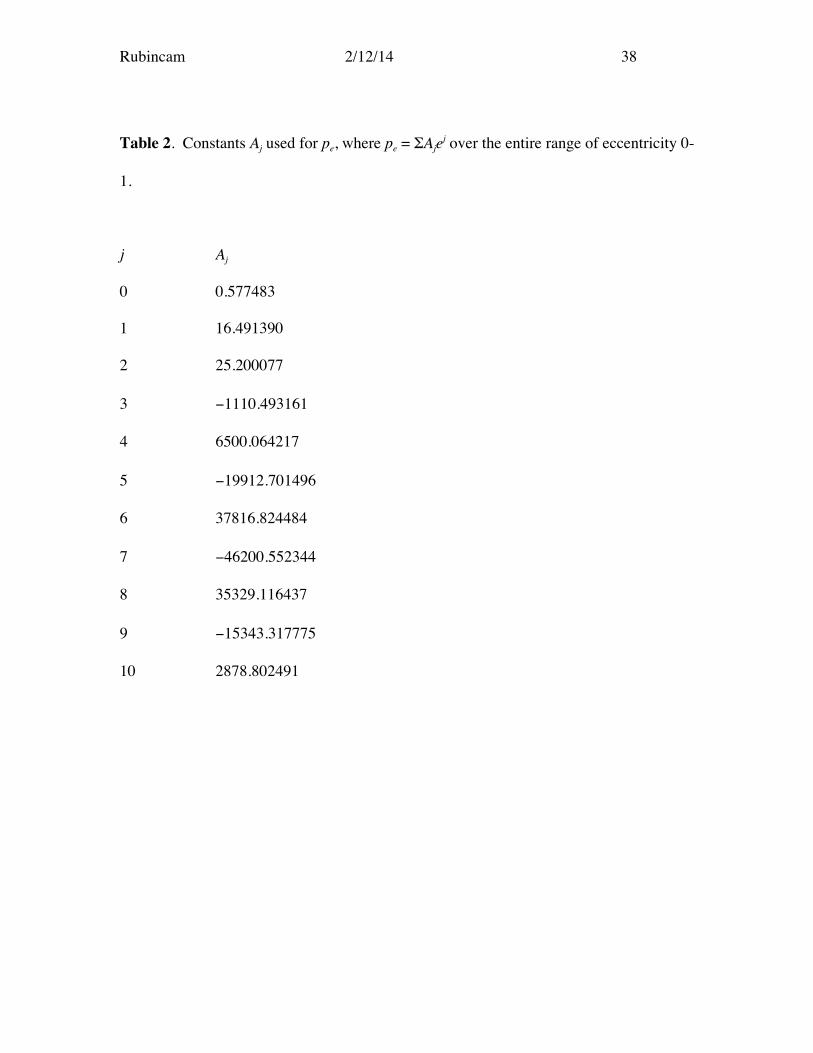
and (8) is satisfied. Figure 4 compares the continuous function (17) with Divine’s

piecewise function. The agreement is quite good. Table 2 gives the values for Aj.

Switching to the dimensionless variable ξ = 2{e − [(r − r1)/ (r + r1)]}1/2, so that e =

[(r − r1)/ (r + r1)] + ξ 2/4, avoids the singularity in the integral over e in (3). The integral

can then easily be numerically integrated.

Finally, there is the integral over r1 in (3) to be evaluated. Unlike pI and pe, the

core and asteroidal populations have their own distinct N1 functions, with the core N1

Rubincam 2/12/14 12

function peaking close to the Sun and the asteroidal N1 function peaking in the main belt

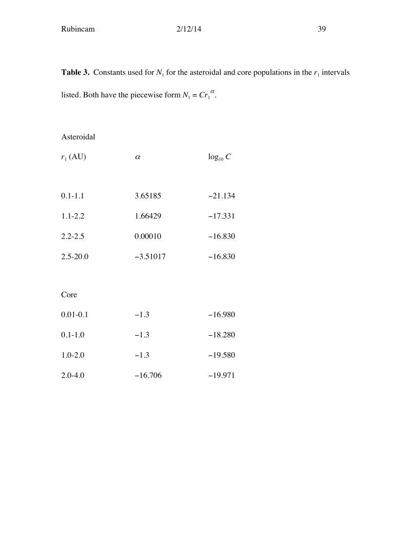
(Fig. 5). Divine gives each N1 distribution the piecewise form

N1 = Cr1α , (18)

which is thus a function of r1, with the constants C and α being given in Table 3. The

problem in this case is that (r − r1)1/2 appears in the denominator, which leads to infinity

problems when r1 is close to r. This singularity in (3) in the integral over r1 can be

avoided by switching to the dimensionless variable ζ = [(r − r1)/r]1/2, so that r1 = r (1 −

ζ2). The resulting expression can easily be numerically integrated.

With the pI, pe, and N1 in hand, ND in (3) can be evaluated. Figure 6 shows ND for

the core and asteroidal populations as found by Divine (straight lines), while the dots are

the ND values computed here for distances between 0.5 AU and 5 AU. The agreement is

quite good.

3. Space erosion due to dust particle impact abrasion

This section computes the rate of space erosion (abrasion) due to dust particle

impacts on the meteoroid. It is first necessary to find the velocity of the dust and of the

meteoroid, so that the relative velocity can be computed. From the relative velocity

comes the kinetic energy which makes the craters.

Let v be the velocity of a dust particle in the inertial frame of Fig. 2. The dust

particle’s velocity is given by

Rubincam 2/12/14 13

v = vrˆ r + vφφ ( ˆ n × ˆ r ) (19)

where vr is the radial speed, vφ is the transverse speed, and ˆ n × ˆ r is the unit vector in the

orbital plane transverse to ˆ r . The Cartesian velocities are given by Divine (1993):

vx = (v ⋅ ˆ x ) =x

rvr −

ryvφ cos I + xzvs

x2 + y2

⎛

⎝ ⎜

⎞

⎠ ⎟ , (20)

vy = (v ⋅ y) =y

rvr +

rxvφ cos I − yzvs

x2 + y2

⎛

⎝⎜

⎞

⎠⎟ , (21)

and

vz = (v ⋅ z) =z

rvr + vs , (22)

where

vr = ±GMS

r 2r1

(r − r1 )[−(r − r1) + (r + r1)e]⎧ ⎨ ⎪

⎩ ⎪

⎫ ⎬ ⎪

⎭ ⎪

1/ 2

, (23)

vφφ = +GM Sr1

r2 (1+ e)⎡

⎣ ⎢ ⎤

⎦ ⎥

1/2

, (24)

Rubincam 2/12/14 14

and

vs = ±vφφ (cos2 λ − cos2 I )1/2 . (25)

Here MS is the mass of the Sun and G is the universal constant of gravitation. Divine

(1993) presents these equations without giving the derivations; an outline of the

derivations is given in the Appendix.

A collision occurs when the meteoroid’s position and the dust particle’s position

coincide. In other words, when they have the same position r ˆ r as given by (1). The

collisions take place at the nodes of the dust particle’s orbit.

Gault et al. (1972) find for polycrystalline rocks that the mass of material Mej

ejected from the surface of the meteoroid in an impact is given by Mej ≈ 8.63 × 10-11 E 1.13

cos2 Θ, where E is the kinetic energy measured in ergs, Mej is in grams, and Θ is the angle

of the velocity vector with the local vertical. Converting Gault et al.’s equation to SI units

gives

Mej ≈ Kstone [mD(Δv)2/2]1.13 cos2 Θ , (26)

where Kstone = 7.015 × 10-6, E = mD(Δv)2/2 is the kinetic energy and is now in joules, and

mD is the mass of the impacting dust particle in kg. Also, Δv is its speed relative to the

meteoroid in m s-1, where

(Δv) 2 = (v - vM) ⋅ (v - vM) ,

Rubincam 2/12/14 15

with vM being the velocity of the meteoroid.

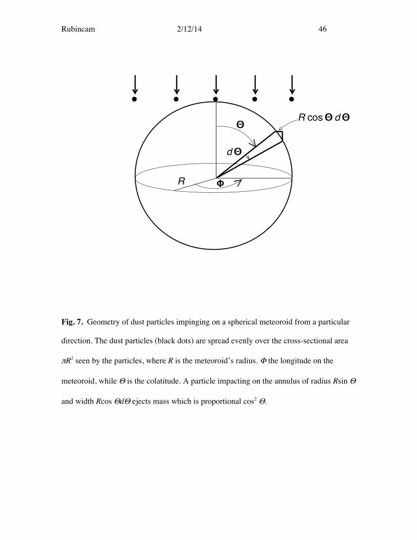
To account for the oblique impacts embodied by cos2 Θ, it will be reasonably

assumed that the dust particles pelting the meteoroid from a particular direction will be

spread uniformly over the circular cross-sectional area seen by the incoming particles.

Considering the number of particles impacting an annulus of radius Rsin Θ and width

Rcos Θ dΘ (Fig. 7) and averaging over the hemisphere pelted by the dust gives

R2 sinΘ cosΘ cos2 Θ dΘ dΦ / R2 sinΘ cosΘ dΘ dΦ =1/ 20

π /2

∫0

2π

∫0

π /2

∫0

2π

∫ (27)

as the factor needed to find the average amount of ejected mass <Mej> :

<Mej> ≈ (Kstone/2)[mD(Δv)2/2]1.13 = nejmD (28)

In the above equation nej is some multiple of the dust particle’s mass and is given by

nej ≈ (Kstone/22.13 )mD

0.13Δv2.26 . (29)

Assuming that mD ≈ 10-6 kg and Δv ≈ 5000 m s-1 give nej ≈ 61 in (29). Thus the mass lost

from the stony meteoroid by making a crater is typically many times greater than the

mass of the impacting dust particle.

Rubincam 2/12/14 16

The amount of mass loss in ejected kilograms per second from a meteoroid of unit

volume (1 m3) is given by

dM

dt unit

= −κ = −(Kstone / 22.13)WD

πw(r1,e, I )(Δv)(Δv)2.26 dr1∫∫∫ dedI (30)

where the extra factor Δv comes from the flux of particles hitting the unit volume and κ

depends on the orbit the meteoroid is in. Also,

WD = mD1.13Hm dmD0

∞

∫ .

Assume a spherical meteoroid of radius R and mass M = 4πρR3/3, where ρ is the density.

To get the rate of mass loss dM/dt (30) is multiplied by πR2. It is also the case that dM/dt

= d(4πρR3/3)/dt = 4πρR2(dR/dt). Equating the two rates gives

dR

dt= −

κ4ρ

= −β . (31)

The quantity dR/dt will be referred to below interchangeably as the space erosion

rate or abrasion rate. It is important to note that it is independent of radius R, as indicated

in (31), and is constant as long as the meteoroid stays in the same orbit. It is assumed that

(31) applies to all stony meteoroids regardless of composition. Stony meteorites range in

Rubincam 2/12/14 17

density from ~2200 kg m-3 to ~3900 kg m-3 (McCall, 1973, p. 149). A value of ρ = 2800

kg m-3 is adopted here.

4. Space erosion rates

Figure 8 shows the time Tmetre to erode 1 meter of a stony meteoroid due to

impacts from the combined asteroidal and core populations for the assumed abrasion

model, where

β = (1 m)/Tmetre , (32)

and where the subscript is the accepted spelling of the SI unit of length. All the meteoroid

orbits lie in the ecliptic; hence IM = 0. The black dots show Tmetre for meteoroids in

circular orbits for semimajor axes aM between 0.5 AU and 3.5 AU. The speediest erosion

times Tmetre occur close to the Sun, where meteoroid velocities are fast and the core ND

concentration is high (Fig. 6). A meteoroid at 0.5 AU takes 50 × 106 y to erode 1 m, while

at 2 AU it is the much longer 430 × 106 y. Beyond 2.5 AU the times increase sharply,

rising to > 1000 × 106 y at 3.5 AU, which is slightly beyond the outer edge of the main

belt.

The square in Fig. 8 is for a stony meteoroid with semimajor axis aM = 2 AU and

eccentricity eM = 0.5, so that the meteoroid journeys between 1 AU to 3 AU; in other

words, between the Earth and the asteroid belt. In this case Tmetre = 126 × 106 y. This is

shorter than for a meteoroid in a circular orbit with the same semimajor axis.

Rubincam 2/12/14 18

The star in Fig. 8 is for a stony meteoroid with aM = 1.75 AU and eM = 0.714, so

that it journeys between 0.6 AU and 3.5 AU. It has the quickest erosion time of all: Tmetre

= 30 × 106 y. It is in an orbit which takes it deep inside the core population at high

velocity, as well as through the asteroidal population in the main belt; hence the short

erosion time.

Iron meteoroids apparently will comminute at a rate ~270 times slower than for

stony meteoroids. The estimate is made as follows. Matsui and Schultz (1984) shot ~0.15

g steel projectiles at an iron meteorite using the NASA Ames Research Center’s Vertical

Gun Range. They found that for speeds of ~5 km s-1, the mass loss was ~2.6 times the

mass of the projectile; in other words nej ≈ 2.6. Assuming for vertical impacts

nej = (Kiron/21.13) mD

0.13 Δv2.26 (33)

by analogy with (26) for mD = 1.5 × 10-4 kg yields Kiron = 7.809 × 10-8 for irons, as

compared to Kstone = 7.015 × 10-6 for stones.

Thus if (33) applies to iron meteoroids, then the mass loss is a factor of ~90

smaller per impact than for stony meteoroids. The density of iron meteoroids is ~7870 kg

m-3, a factor of ~3 larger than for stones. Hence the space erosion rate β for irons by (31)

would be ~270 slower than for stones. Such slow rates are not shown in Fig. 8 and iron

meteoroids would barely erode over the age of the solar system, according to the present

abrasion model.

Rubincam 2/12/14 19

5. Space erosion rate and CRE ages of stony meteorites

How do the erosion times Tmetre in Fig. 8 relate to the CRE ages of stones? Several

simplifications are made below to give a rough answer to this question.

While Fig. 8 shows Tmetre for two elliptical orbits and similar orbits could be

calculated, only the Tmetre for circular orbits are used here to estimate CRE ages. The

rationale is that a meteoroid originating in the main belt spends little time in an elliptical

orbit (Gladman et al., 1997) before impacting the Earth, offsetting the increased erosion

rate.

In what follows below the cosmic ray flux is assumed to be isotropic and constant

in space and time throughout the solar system. Also, meteoroids always remain spherical

regardless of size as they erode away.

CRE ages are measured through the accumulation of products created from the

galactic cosmic ray bombardment. The product concentration varies with depth inside a

meteoroid. Neon is an example and is the only cosmic ray product examined here.

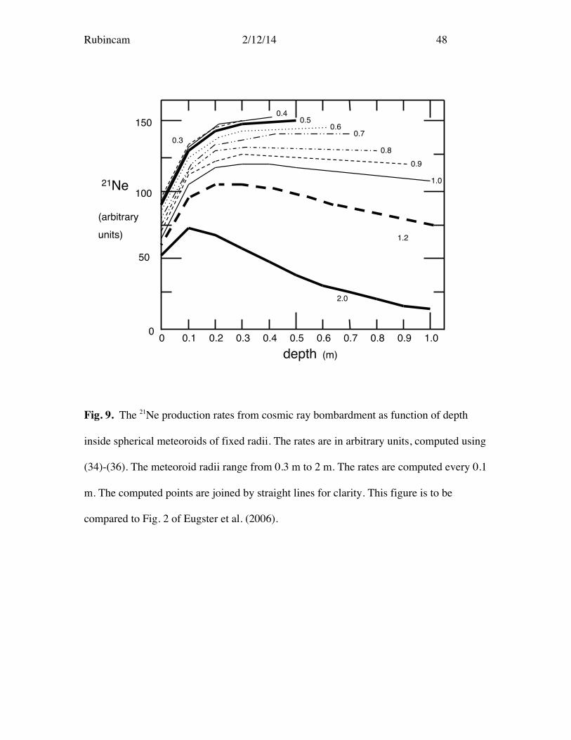
Eugster et al. (2006) in their Fig. 2 show the production rates with depth of 21Ne for stony

spherical meteoroids for several fixed radii. For a stony spherical meteoroid whose radius

remains constant, the 21Ne production rate slowly increases from the meteoroid’s center,

and then sharply decreases as the surface is neared.

Eugster et al.’s curves can be approximated by the equations

PNe = [ANe + BNe(1− e−d /γ )]e−d /Γ . (34)

Here PNe is the production rate of 21Ne in arbitrary units per 106 y, BNe = 63, and

Rubincam 2/12/14 20

ANe = 50 + 355R e−R/s , (35)

where R is the meteoroid’s radius in meters, d is the depth below the surface in meters, s

= 0.333 m, and γ = 0.1 m. Also,

1

Γ= CNe{1+ tanh[h(R − Rh )]} , (36)

where CNe = 1.111, h = 2.519, and Rh = 1.4455. The resulting curves using (34)-(36) are

shown in Fig. 9 and are to be compared with Eugster et al.’s Fig. 2. The rates are

computed every 0.1 m in depth. The computed points in Fig. 9 are joined by straight lines

for clarity. Equations (34)-(36) and their associated constants are not based on any

theory; rather, they are the result of trial-and-error and mimic Eugster et al.’s curves

reasonably well for R ≥ 0.3 m.

Suppose that a meteoroid undergoes no abrasion, so that its radius stays fixed. In

this case the 21Ne concentration simply increases linearly with time at any given point,

and the concentration at any given instant looks the same as the production rate in Fig. 9;

only the scale and units of the vertical axis change. On the other hand, for a meteoroid

which does undergo space erosion, the production rate (34) holds at every instant, but the

meteoroid’s radius is constantly changing, resulting in curves that do not reproduce the

curves in Fig. 9. What the concentration curves do look like is taken up next.

Rubincam 2/12/14 21

A computer program used (34)-(36) to compute the concentration inside a

spherical stony meteoroid whose radius R shrinks at a constant rate due to abrasion:

R = R0 − βt = R0 − (1 m/Tmetre)t . (37)

In this equation R0 = 5 m is the initial radius at time t = 0. This value of R0 was chosen

because it is large enough to greatly shield the interior more than 3 m deep from the

cosmic rays. The time step was 106 y.

Figure 10 shows the results for Tmetre = 430 × 106 y, which is the value for a stone

in a circular ecliptic orbit at 2 AU (Fig. 8), and gives the fastest erosion rate in the main

asteroid belt for circular orbits. The thin lines are the concentrations vs. depth for a

shrinking meteoroid when the radius reaches R = 2 m, 1 m, 0.5 m, and then 0.3 m. The

thick lines are the corresponding concentrations for fixed radii at these values of R; the

exposure times τNe associated with the thick lines are chosen to give concentrations which

roughly agree with the thin lines at approximately half the radius of the meteoroid. The

smallest value τNe = 176 × 106 y in Fig. 10 occurs for stones which have radii R > ~1 m,

but thereafter the values rapidly increase as the meteoroid shrinks, rising to 384 × 106 y

for a 0.3 m meteoroid. It is of interest that for meteoroids with R > ~1 m the following

relationship holds:

τNe ≈ c1Tmetre , (38)

where c1 ≈ 0.41. For R < ~1 m, the value of c1 rises as the radius shrinks.

Rubincam 2/12/14 22

The shapes of the space erosion curves are quite different at shallow depths from

those for meteoroids of fixed radii. Moving from right to left in Fig. 10, the eroding

meteoroids have curves which increase or flatten out when nearing the surface, while

those of fixed radii show a sharp downturn. Hence according to the present model,

pristine meteoroids recovered in space will not show the downturn if they have eroded

from a large body.

Meteoroids can ablate and fragment perhaps as much as 27%-99% of their mass

during their passage through the Earth’s atmosphere (Eugster et al. 2006, p. 833). If a

meteoroid loses its outermost 0.1−0.2 m, then the part of the curve where the downturn is

expected vanishes. An investigator may not realize the downturn never existed because of

space erosion, and may take τNe as the CRE age and erroneously assume that the

meteoroid was liberated from deep within an asteroid a time τNe years ago, when in fact

the meteoroid could have been an independent larger body for a long time and taken

longer than τNe to drift to a resonance.

If the τNe of eroding meteoroids are taken to be their CRE ages, then is the

assumed space erosion model in any sort of disagreement with the measured CRE ages of

meteorites? This question speaks to the first of the two issues raised in the Introduction.

If, as an extreme example, space erosion was so fast that the erosion τNe values

were only on the order of ~1 × 106 y, then a meteoroid would not have enough time to

accumulate sufficient 21Ne to account for the observed longer ~30 × 106 y ages and there

would be a problem. The least upper bound on τNe is ~176 × 106 y for meteoroids ~1 m in

radius (Fig. 10) and larger. This limit tends to agree with what is observed: most stony

Rubincam 2/12/14 23

meteorites have ages < ~100 × 106 y. Thus it may be that space erosion sets upper limits

on the CRE ages of stones which originate in the asteroid belt, but the limits are

comfortably high enough to encompass the measured CRE ages, which are presumably

due to Yarkovsky drift.

The time Tmetre to erode 1 m of the surface of a hypothetical rocky and regolith-

free Near-Earth asteroid (NEA) in the same orbit as the Earth is ~300 × 106 y. This would

lead to τNe = ~120 × 106 y for the assumed model. This value of Tmetre = ~300 × 106 y at 1

AU is in fair agreement with one estimate of the abrasion rate of lunar rocks. Gault et al.

(1972, p. 2723) find ~1mm/106 y for an assumed 1.5π steradian exposure for a rock on

the Moon’s surface. Adjusting this rate for the 4π exposure of a meteoroid gives Tmetre =

~375 × 106 y, which is close to the value found here.

An improved space erosion model might increase the abrasion rate so that the τNe

actually drop into the observed range of CRE values, rather than just set upper limits.

This would have implications for Yarkovsky drift. What happens in this case is discussed

in the next section.

6. Yarkovsky or space erosion?

Space erosion appears to place upper limits on meteoroid CRE ages, meaning that

the ages can be less, but not more. So if the Yarkovsky drift to the resonances limit stony

meteoroid CRE ages to, say, the ~30 × 106 y observed for L chondrites (e.g., McSween,

1999, p. 246), and the abrasion least upper bound is ≤ ~176 × 106 y as in Fig. 10, then

Rubincam 2/12/14 24

there is no problem with the standard Yarkovsky scenario of how many meteoroids get

their CRE ages. The ages tend to be a factor of 6 younger than the least upper bound.

But the factor of 6 is small enough to give pause. If the space erosion rates were

great enough to give τNe = ~30 × 106 y, and if the measured CRE ages of many stony

meteorites are also ~30 × 106 y, then space erosion may compete with Yarkovsky.

It might even call into question whether Yarkovsky drift is the mechanism by

which meteoroids reach the resonances. Meteoroids could theoretically dawdle in the

asteroid belt for very long times using other mechanisms to journey to the resonances, but

always turn in the observed CRE ages, thanks to space erosion.

In other words, is something wrong with Yarkovsky? Does it really operate at the

expected level? If not, why not?

The ages computed here are based on a number of assumptions, and the calculated

CRE ages could go up or down using a different set of assumptions. If the ages go down

by a factor of ~6, then Yarkovsky could be in trouble. Hence the assumptions are worth

examining to see if the factor of 6 is within reach.

Several ways to get a greater space erosion rate immediately come to mind. The

most obvious is to simply raise the dust mass upper limit. Divine (1993) conveniently put

the upper limit at 1 g = 10-3 kg, a size much larger than what is ordinarily considered

“dust” (e.g., Shirley, 1997). The present discussion retains Divine’s upper limit of 1 g;

adding in bigger impactors would certainly excavate more material than considered here.

This would give faster erosion, but gets into the statistics of small numbers and

fracturing.

Rubincam 2/12/14 25

Abrasion is at one end of a continuum, with catastrophic disruption at the other

end. Possibly many CRE ages might be controlled by the in-between process of spallation

and abrasion (Fujiwara et al., 1977), rather than just abrasion alone. Because small

impactors are more numerous than large ones, spallation will presumably be more

common than catastrophic disruption, in which many fragments of all sizes are created.

For instance, Matsui and Schultz (1984) found that iron meteorites sometimes fractured

when hit by a 0.00015 kg (0.15 g) steel impactor. Splintering off sizeable pieces, rather

than cratering, may be a way of eroding an iron meteoroid faster than the rates found

here. On the other hand, Matsui and Schultz found that basaltic impactors did not create

fractures at the speeds they used. Moreover, it is not clear that chunks chipped off by

spallation would mimic the steady erosion that the sand-blasting by abrasion might be

expected to give, unless the chunks were numerous and relatively small.

A second obvious way to get faster erosion is to tinker with Divine’s populations.

Grün and P. Staubach (1996) verify that Divine’s five solar system dust populations fit

lunar cratering, spacecraft, and zodiacal light data. But the populations, including the

asteroidal and core populations considered here, are nonunique (Divine, 1993, pp.

17,032-17,033) and model-dependent (Divine, 1993 p. 17,037). Hence further

information about the asteroidal population could increase or decrease the dust

concentration, with a corresponding effect on CRE ages.

An alternative distribution for the asteroidal N1 population invented for the sake

of argument is shown in Fig. 5. It extends the trend in the inner solar system to 3 AU

(dotted line), and then turns down and cuts off at 5 AU. The resulting Tmetre for circular

orbits are shown as the open circles in Fig. 8. No open circles are visible in the figure for

Rubincam 2/12/14 26

aM ≤ 1.5 AU because they virtually coincide with the solid black circles. But the Tmetre are

dramatically lower than from Divine’s population at 2 AU and beyond, so much so that

the Yarkovsky interpretation for stones might be in trouble if this or a similar alternative

distribution were to hold.

However, Divine (1993, p. 17,037) states that a dust distribution which continues

the trend in the inner solar system would make too large a contribution to the zodiacal

light for his assumed geometric albedo of 0.01. Hence adopting the alternative

distribution may not be viable. Further, a more accurate distribution than Divine’s might

just as well decrease the dust concentration as increase it.

There is also the question as to whether the dust populations have stayed constant

over time. It is assumed here that they have stayed the same over hundreds of millions of

years. However, the dust populations have presumably varied over geologic time, as

reflected in the dust influx to the Earth (e.g., Gault et al., 1972; Peucker-Ehrenbrink,

2001; Mukhopadhyay et al., 2001). The present influx may be twice the average influx

over the past 70 × 106 y (Farley, 2001, p. 1194), so that the abrasion rates may be smaller

than found above. On the other hand, collisions in the asteroid belt may yield temporary

local dense concentrations of dust which would accelerate space erosion there.

Further, the present model assumes a constant flux over geologic time for the

galactic cosmic rays. This may not be the case (e.g., Eugster et al., 2006).

A final obvious way to get a greater abrasion rate is to assume more material is

lifted off from microcratering than given by (29) and (33). Low temperatures in the

asteroid belt may make the rock more brittle, thus increasing the mass loss beyond what

is given by (29) and (33).

Rubincam 2/12/14 27

So: can the model be reasonably altered enough to accommodate the factor of ~6

and cast doubt on Yarkovsky? As shown above, arguments can be adduced to either

increase or decrease the space erosion rate. At the present time the question remains

open.

7. Discussion

Only 21Ne concentrations are examined here in relation to CRE ages. It was more

or less assumed that τNe equates with CRE age. Neither other cosmic ray products, such

as 3He, nor tracks are considered in relation to the space erosion model.

All rocky surfaces in the solar system which remain free of regolith may have the

upper limit on their CRE ages controlled by space erosion. The particular limits depend

upon the dusty environment they find themselves in, as shown in Fig. 8. Erosion rates

inside 1 AU are rapid. Such fast erosion might have implications for the CRE ages of

regolith-free Near-Earth Asteroids (NEAs) and any meteorites which originate from them

(Morbidelli et al., 2006). Pristine samples returned from an NEA may not show the

downturn in the 21Ne concentration as the surface is neared (Fig. 10).

The presence of regolith could impede the abrasion of the monolithic rock

underneath by being thick enough to intercept the dust bombardment, but perhaps still be

thin enough to allow the cosmic rays to penetrate the rubble and age what is below.

Presumably meteoroids and the smallest asteroids are regolith-free.

On the issue of whether space erosion or Yarkovsky controls CRE ages, the

Yarkovsky effects depend on principal axis rotation. The diurnal Yarkovsky effect

Rubincam 2/12/14 28

depends on the meteoroid’s sense of rotation, increasing the semimajor axis for prograde

rotation and decreasing it for retrograde rotation. The YORP effect (e.g., Paddack, 1969;

Paddack and Rhee, 1975; Rubincam, 2000; Bottke et al., 2002; Vokrouhlicky et al., 2006;

Statler, 2009) or collisions might change the spin axis orientation enough to lessen

diurnal Yarkovsky’s effectiveness by a random walk, but the seasonal Yarkovsky effect

(Rubincam, 1987, 1995) will still be operative regardless of where the spin axis is, unless

the meteoroid tumbles most of the time, which seems unlikely.

At the young end of the CRE age distribution, it is hard to see how space erosion

could explain the shortest observed ages of ≤ ~106 y regardless of how much the abrasion

rate is increased. (Yarkovsky also has trouble with such young ages; Morbidelli et al.,

2006). Moreover, an improved model might just as well lower abrasion rates as raise

them. Further research is needed to see whether space erosion casts doubt on the

hypothesis that Yarkovsky drift to the resonances controls many meteorite CRE ages.

At the other end of the CRE age distribution, the aubrites also pose a problem for

space erosion controlling stony CRE ages. They are fragile but tend to have long ages. A

possible way to resolve the problem is if the aubrite parent body is in an orbit inclined to

the ecliptic, which would lessen collisional encounters (McSween, 1999, p. 247). Inclined

orbits are not considered here.

The iron meteoroids have the oldest CRE ages and present another possible

obstacle. Their abrasion rates appear to be so slow that they undergo little erosion

(Matsui and Schultz, 1984 and section 4 above), so that their CRE ages might be

controlled by Yarkovsky. Thus there would be two separate explanations as to how

Rubincam 2/12/14 29

meteorites get their CRE ages: space erosion for stones and Yarkovsky for irons, rather

than one elegant unifying explanation.

A potential way around the iron problem is the combined abrasion and fracturing

mentioned in section 6. Irons might “erode” mainly by spallation (Matsui and Schultz,

1984), which might explain their CRE ages, rather than Yarkovsky.

The results above cast some doubt on the Yarkovsky interpretation of meteorite

CRE ages. More research is needed to clarify the issue.

Appendix

Divine (1993) gives the correct expressions for the dust particle speeds vφ, vr, vs,

and vx, vy, vz, but does not derive them. The purpose of this appendix is to outline their

derivation, in order to save readers time when it comes to verifying the equations for

themselves.

The velocity of the dust particle is given by (19). The speed vφ is most easily

found first. By Kepler’s law r 2(dφ/dt) = [GMS a(1 - e 2)]1/2, where φ is the angle in the

orbital plane. Using the relation r1 = a(1 - e) to eliminate semimajor axis a yields vφ = r

(dφ/dt) = +[GMSr1(1+e)/r 2]1/2, which agrees with (24). The radial speed vr can then be

found from vr2 = ±(v 2 - vφ

2)1/2 and the energy relation v 2 = GMS [(2/r) - (1/a)] after once

again eliminating a, yielding (23).

Finding vs is harder work. By (1)-(2) and (19)

Rubincam 2/12/14 30

vφ (n × r) ⋅ x

= -vφ [(z/r) sin I cos Ω + (y/r) cos I], (A1)

vφ (n × r) ⋅ y

= vφ [(x/r) cos I - (z/r) sin I sin Ω], (A2)

vs = vφ (n × r) ⋅ z

= vφ [(y/r) sin I sin Ω + (x/r) sin I cos Ω] (A3)

Also, because ˆ n is perpendicular to ˆ r

n ⋅ r = (x/r) sin I sin Ω - (y/r) sin I cos Ω + (z/r) cos I = 0 (A4)

Squaring (A3) results in a term containing 2xy times some other factors. Squaring (A4)

also contains in the same 2xy term. Using the square of (A4) to eliminate the 2xy term in

vs2 ultimately results in the desired result vs

2 = vφ2(cos2 λ - cos2 I), which is the square of

(25), after using sin λ = z/r to get rid of z. This completes finding vφ, vr, and vs.

The expressions for vx, vy, and vz will be found next. The velocity vector is given

by (19). The first term on the right-hand side of (20), (21), and (22) is clearly the

Cartesian component of vrˆ r ; it remains to find the Cartesian components of vφ (ˆ n × ˆ r ) .

Rubincam 2/12/14 31

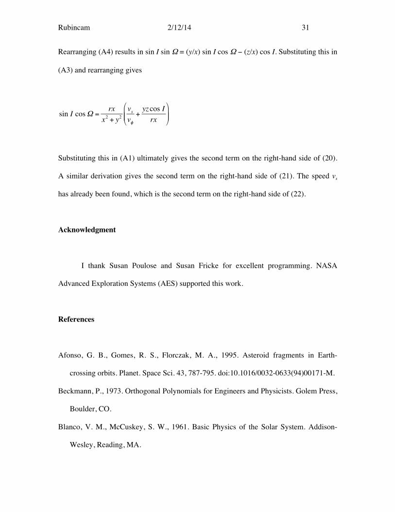
Rearranging (A4) results in sin I sin Ω = (y/x) sin I cos Ω − (z/x) cos I. Substituting this in

(A3) and rearranging gives

sin I cos Ω =rx

x2 + y2

vs

vφ

+yz cos I

rx

⎛

⎝ ⎜ ⎜

⎞

⎠ ⎟ ⎟

Substituting this in (A1) ultimately gives the second term on the right-hand side of (20).

A similar derivation gives the second term on the right-hand side of (21). The speed vs

has already been found, which is the second term on the right-hand side of (22).

Acknowledgment

I thank Susan Poulose and Susan Fricke for excellent programming. NASA

Advanced Exploration Systems (AES) supported this work.

References

Afonso, G. B., Gomes, R. S., Florczak, M. A., 1995. Asteroid fragments in Earth-

crossing orbits. Planet. Space Sci. 43, 787-795. doi:10.1016/0032-0633(94)00171-M.

Beckmann, P., 1973. Orthogonal Polynomials for Engineers and Physicists. Golem Press,

Boulder, CO.

Blanco, V. M., McCuskey, S. W., 1961. Basic Physics of the Solar System. Addison-

Wesley, Reading, MA.

Rubincam 2/12/14 32

Bottke, W. F., Rubincam, D. P., Burns, J. A., 2000. Dynamical evolution of main belt

meteoroids:numerical simulations incorporating planetary perturbations and

Yarkovsky thermal forces. Icarus 145. 301-331. doi: 10.1006/icar.2000.6361

Bottke, W. F., Vokrouhlicky, D., Rubincam, D. P., Broz, M., 2002. Dynamical evolution

of asteroids and meteoroids using the Yarkovsky effect. In: Bottke, W. F., Cellino,

A., Paolicchi, P., Binzel, R. (Eds.), Asteroids III, Univ. of Arizona Press, Tucson, AZ,

pp. 395-408.

Buchwald, V. F., 1975. Handbook of Iron Meteorites. Univ. of California Press,

Berkeley, CA.

Divine, N., 1993. Five populations of interplanetary meteoroids. J. Geophys. Res. 98,

17,029-17,048. doi: 10.1029/93JE01203.

Eugster, O., Herzog, G. F., Marti, K., Caffee, M. W., 2006. Irradiation records, cosmic-

ray exposure ages, and transfer times of meteorites. In: Lauretta, D. S., McSween, H.

Y. (Eds.), Meteorites and the Early Solar System II, Univ. of Arizonz Press, Tucson,

AZ, pp. 829-851.

Farinella, P., Vokrouhlicky, D., 1999. Semimajor axis mobility of asteroidal fragments.

Science 283, 1507-1510. doi: 10.1126/science.283.5407.1507.

Farley, K. A., 2001. Extraterrestrial helium in seafloor sediments: Identification,

characteristics, and accretion rate over geologic time. In: Peucker-Ehrenbrink, B.,

Schmitz, B. (Ed.s), Accretion of Extraterrestrial Matter Throughout Earth’s History.

Kluwer Academic/Plenum Publishers, New York, pp. 179-204.

Fisher, D. E., 1961. Space erosion of the Grant meteorite. J. Geophys. Res. 66, 1509-

1511. doi: 10.1029/JZ066i005p01509.

Rubincam 2/12/14 33

Fujiwara, A., Kamimoto, G., Tsukamoto, A., 1977. Destruction of basaltic bodies by

high-velocity impact. Icarus 31, 277-288. doi: 10.1016/0019-1035(77)90038-0.

Gault, D. E., Hörz, F., Hartung, J. B., 1972. Effects of microcratering on the lunar

surface. Proc. Third Lunar Sci. Conf., Vol. 3, pp. 2713-2734.

Gladman, B. J., Migliorini, F., Morbidelli, A., Zappala, V., Michel, P., Cellino, A.,

Froeschle, C., Levison, H. F., Bailey, M., and Duncan, M., 1997. Dynamical lifetimes

of objects injected into asteroid belt resonances. Science 277, 197-201. doi:

10.1126/science.277.5323.197.

Greenberg, R., and Nolan, M. C., 1989. Delivery of asteroids and meteorites to the inner

solar system. In Binzel, R. P., Gehrels, T., Matthews, M. S. (Ed.s), Asteroids II, Univ.

of Arizona Press, Tucson, AZ, 778-804.

Grün, M. J., Staubach, P., 1996. Dynamic populations of dust in interplanetary space. In:

Gustafson, B. A. S., and Horner, M. S. (Ed.s), Physics, Chemistry, and Dynamics of

Interplanetary Dust. ASP Conference Series, vol. 104, Astron. Soc. Pacific, pp. 15-18.

Hughes, D. W., 1982. Meteorite erosion and cosmic ray variation. Nature 295, 279-280.

doi: 10.1038/295279a0.

Matney, M. J., Kessler D. J., 1996. A reformulation of Divine’s interplanetary model. In:

Gustafson, B. A. S., and Horner, M. S. (Ed.s), Physics, Chemistry, and Dynamics of

Interplanetary Dust. ASP Conference Series, vol. 104, Astron. Soc. Pacific, pp. 15-18.

Matsui, T., Schultz, P. H., 1984. On the brittle-ductile behavior of iron meteorites: new

experimental constraints. LPSC, XV, 519-520.

McCall, G. J. H., 1973. Meteorites and Their Origin. Wiley, New York.

Rubincam 2/12/14 34

McSween, H. Y., 1999. Meteorites and Their Parent Bodies, 2nd. ed., Cambridge Univ.

Pr., New York.

Morbidelli, A., Gounelle, Levison, H. F., Bottke, W. F., 2006. Formation of the binary

near-Earth object 1996 FG3: Can binary NEOs be the source of short-CRE

meteorites? Meteoritics Plan. Sci. 41, 875-887.

Mukhopadhyay, S., Farley, K. A., Montanari, A., 2001. A 35 Myr record of helium in

pelagic limestones from Italy: Implications for interplanetary dust accretion from the

early Maastrichtian to the middle Eocene. Geochim. Cosmochim. Acta 65, 653-669.

doi:10.1016/S0016-7037(00)00555-X.

Nakamura, A. M., Fijiwara, A., and Kadono, T., 1994. Velocity of finer fragments from

impact. Planet. Space. Sci. 42, 1043-1052. doi: 10.1016/0032-0633(94)90005-1.

Norton, O. R., 1994. Rocks from Space. Mountain Press, Missoula, Montana.

Nunes, J. A., 1994. In memoriam: T. Neil Divine (1939-1994). Icarus 109, 2. doi:

10.1006/icar.1994.1073.

O’Keefe, J. A., 1976. Tektites and Their Origin. Elsevier, New York.

Öpik, E. J., 1951. Collision probabilities with the planets and the distribution of

interplanetary matter. Proc. R. Irish Acad. 54A, 165-199.

Paddack, S. J., 1969. Rotational bursting of small celestial bodies: Effects of radiation

pressure. J. Geophys. Res. 74, 4379-4381. doi: 10.1029/JB074i017p04379.

Paddack, S. J., Rhee, J. W., 1975. Rotational bursting of interplanetary dust particles.

Geophys. Res. Lett. 2, 365-367. doi: 10.1029/GL002i009p00365.

Peterson, C., 1976. A source mechanism for meteorites controlled by the Yarkovsky

effect. Icarus 29, 91-111. doi: 10.1016/0019-1035(76)90105-6.

Rubincam 2/12/14 35

Peucker-Erenbrink, B., 2001. Iridium and osmium as tracers of extraterrestrial matter in

marine sediments. In: Peucker-Ehrenbrink, B., Schmitz, B. (Ed.s), Accretion of

Extraterrestrial Matter Throughout Earth’s History. Kluwer Academic/Plenum

Publishers, New York, pp. 163-178.

Rubincam, D. P. 1987. LAGEOS orbit decay due to infrared radiation from earth. J.

Geophys. Res. 92, 1287-1294. doi: 10.1029/JB092iB02p01287.

Rubincam, D. P., 1995. Asteroid orbit evolution due to thermal drag. J. Geophys. Res.

100, 1585-1594. doi: 10.1029/94JE02411.

Rubincam, D. P., 2000. Radiative spin-up and spin-down of small asteroids. Icarus 148,

2-11. doi: 10.1006/icar.2000.6485.

Selby, S. M., 1974. CRC Standard Mathematical Tables, 22nd ed., CRC Press,

Cleveland, OH.

Shaeffer, O. A., Nagel, K., Fechtig, H., Neukum, G., 1981. Space erosion of meteorites

and the secular variation of cosmic rays (over 109 years). Planet. Space Sci. 29, 1109-

1118. doi: 10.1016/0032-0633(81)90010-6.

Shirley, J. H., 1997. Dust. In: Shirley, J. H., Fairbridge R. W. (Ed.s), Encyclopedia of

Planetary Sciences, Chapman & Hall, New York, pp. 189-192.

Statler, T. S., 2009. Extreme sensitivity of the YORP effect to small-scale topography.

Icarus 202, 502-513. doi: 10.1016/j.icarus.2009.03.003.

Vokrouhlicky, D., Nesvorny, D., Bottke, W. F., 2006. Seculat spin dynamics of inner

main-belt asteroids. Icarus 184, 1-28. doi: 10.1016/j.icarus.2006.04.007.

Rubincam 2/12/14 36

Welten, K. C., Nishiizumi, K., Caffee, M. W., Schultz, L., 2001. Update on exposure

ages of diogenites: The impact and evidence of space erosion and/or collisional

disruption of stony meteoroids. Meteoritics & Planet. Sci. 36, supplement, A223.

Whipple, F. L., 1962. Meteorite erosion in space. Astron. J. 67, 285. doi:

10.1086/108864.

Whipple, F. L., Fireman, E. L., 1959. Calculation of erosion in space from the cosmic-ray

exposure ages of meteorites. Nature 183, 1315. doi:10.1038/1831315a0.

Wieler, R., Graf, T., 2001. Cosmic ray exposure: History of meteorites. In: Peucker-

Ehrenbrink, B., Schmitz, B. (Ed.s), Accretion of Extraterrestrial Matter Throughout

Earth’s History. Kluwer Academic/Plenum Publishers, New York, pp. 221-240.

Wisdom, J., 1987. Chaotic dynamics in the solar system. Icarus 72, 241-275. doi:

10.1016/0019-1035(87)90175-8.

Wood, J. A., 1968. Meteorites and the Origin of the Planets. McGraw-Hill, New York.

Rubincam 2/12/14 37

Table 1. Constants used in pI, which has the piecewise form pI = c + b cos I in the various intervals for I.

I c b

0-10° 0.0 −0.173725

10-20° −34.441201 37.741467

20-30° −0.0862278 10.082696

30-40° −8.449943 1.321211

45-60° −0.173725 0.347451

60-180° 0.0 0.0

Rubincam 2/12/14 38

Table 2. Constants Aj used for pe, where pe = ΣAjej over the entire range of eccentricity 0-

1.

j Aj

0 0.577483

1 16.491390

2 25.200077

3 −1110.493161

4 6500.064217

5 −19912.701496

6 37816.824484

7 −46200.552344

8 35329.116437

9 −15343.317775

10 2878.802491

Rubincam 2/12/14 39

Table 3. Constants used for N1 for the asteroidal and core populations in the r1 intervals

listed. Both have the piecewise form N1 = Cr1α.

Asteroidal

r1 (AU) α log10 C

0.1-1.1 3.65185 −21.134

1.1-2.2 1.66429 −17.331

2.2-2.5 0.00010 −16.830

2.5-20.0 −3.51017 −16.830

Core

0.01-0.1 −1.3 −16.980

0.1-1.0 −1.3 −18.280

1.0-2.0 −1.3 −19.580

2.0-4.0 −16.706 −19.971

Rubincam 2/12/14 40

Fig. 1. The space erosion scenario. A clock inside a meteoroid measures the cosmic ray

exposure (CRE) age. Left: The CRE clock is initially too deeply buried to be reached by

cosmic rays (thin lines) and the clock face reads zero. Center: Once the surface erodes

enough from dust impacts (dots) so that it is about a meter from the clock, the clock starts

ticking. Right: The CRE clock records its maximum age when the eroding surface

reaches it.

Rubincam 2/12/14 41

Fig. 2. Geometry of a dust particle orbit. The unit vectors ˆ x , ˆ y ,and ˆ z form a right-

handed coordinate system, with ˆ z being normal to the ecliptic. The unit vector ˆ n is

normal to the orbital plane and makes an angle I with ˆ z . The ascending node of the

orbital plane makes an angle Ω in the ecliptic. The perihelion distance is r1. The particle

is at r ˆ r , where ˆ r is the unit position vector and r is the distance from the Sun.

Rubincam 2/12/14 42

Fig. 3. Graph of pI vs. I, which is the same for the core and asteroidal populations.

Divine’s (1993) piecewise function of the form c + bI is given by the solid lines. The dots

show the values of the piecewise function used here, which has the form c + bcos I.

Rubincam 2/12/14 43

Fig. 4. Graph of pe vs. e, which is the same for the core and asteroidal populations.

Divine’s (1993) piecewise function is given by the solid lines. The dots show the values

of the polynomial function in e used here, as given by (17).

Rubincam 2/12/14 44

0� r1 (AU) � �

N1�

1.0 �

-16�

0.1 � 10 �0.2 � 2 �

-18�

-20�

-22�

-24�

0.5 � 5 � 20 �0.05 �

(m-3)�

Fig. 5. The solid lines are Divine’s (1993) dust number concentration N1 for the core and

asteroidal populations as a function of perihelion distance r1 from the Sun. The dotted

line between 1 AU and 5 AU is an alternative concentration to Divine’s: it continues

Divine’s slope, followed by a downturn and cut-off at 5 AU.

Rubincam 2/12/14 45

0� r (AU) � �

N�

1.0 �0.1 � 10 �0.2 � 2 �

-11�

-13�

-14�

-16�

0.5 � 5 � 20 �0.05 �

(m-3)�

-12�

-15�

3 �

D�

Fig. 6. Dust number concentration ND in the ecliptic as a function of distance r from the

Sun for both the core and asteroidal populations for dust particles with masses > 10-7 kg.

Divine’s (1993) concentrations are given by the solid lines. The dots are the values

computed as described in section 2 for 0.5 AU ≤ r ≤ 5 AU.

Rubincam 2/12/14 46

�

d�

R�

Θ

Θ

� � � � �

Φ

R cos�Θ Θ d�

Fig. 7. Geometry of dust particles impinging on a spherical meteoroid from a particular

direction. The dust particles (black dots) are spread evenly over the cross-sectional area

πR2 seen by the particles, where R is the meteoroid’s radius. Φ the longitude on the

meteoroid, while Θ is the colatitude. A particle impacting on the annulus of radius Rsin Θ

and width Rcos ΘdΘ ejects mass which is proportional cos2 Θ.

Rubincam 2/12/14 47

Tmetre�

4 � 0� aM (AU)� �

3 �

1200�

800�

400�

2 �1 �

(106 yr)�

Fig. 8. The time Tmetre required to erode a meter of a stony meteoroid from dust impacts

as a function of a meteoroid’s orbital semimajor axis aM for I = 0°. The solid circles are

for circular orbits, the square gives Tmetre for aM = 2 AU and eM = 0.5, and the star gives

the value for aM = 1.75 AU and eM = 0.714, all using Divine’s populations. The open

circles give the values for circular orbits using Divine’s core population plus the

alternative asteroidal population shown in Fig. 5.

Rubincam 2/12/14 48

0.5 �depth (m)�

100�

0.2 �

�21Ne �

0� 1.0 �

50�

0�

150�

(arbitrary�

units)�

0.7 �

1.2�

0.5� 0.6�

0.9�

1.0�

0.4�

0.3�

2.0�

0.8�

0.7�

0.3 �0.1 � 0.9 �0.8 �0.6 �0.4 �

Fig. 9. The 21Ne production rates from cosmic ray bombardment as function of depth

inside spherical meteoroids of fixed radii. The rates are in arbitrary units, computed using

(34)-(36). The meteoroid radii range from 0.3 m to 2 m. The rates are computed every 0.1

m. The computed points are joined by straight lines for clarity. This figure is to be

compared to Fig. 2 of Eugster et al. (2006).

Rubincam 2/12/14 49

1.0 �depth (m)�

100�

0.5 �

�

21Ne �

0� 2.0 �

200�

0�

400�

τ = 176 × 106�

τ = 302 × 106� Ne�

(arbitrary�

units)�

1.5 �

τ = 176 × 106� Ne�

Ne�

T = 430 × 106�

500�

τ = 384× 106�

Ne�

metre�

300�

600�

Fig. 10. The 21Ne concentrations from cosmic ray bombardment as function of depth

inside a spherical meteoroid in a circular orbit at 2 AU undergoing space erosion, for an

initial radius of 5 m and Tmetre = 430 × 106 y. The concentrations are in arbitrary units,

and are computed every 0.1 m. The computed points are joined by straight lines for

clarity. The thin lines are for when a shrinking meteoroid’s radius reaches 2 m, 1 m, 0.5

m, and 0.3m. The thick lines are corresponding concentrations for meteoroids whose

sizes remain constant at these values of radius. The exposure times τNe associated with the

thick lines are chosen to give concentrations which roughly agree with the thin ones at

approximately half the radius. The eroding meteoroid does not show a downturn in

concentration as the surface is neared, but a non-eroding meteoroid would.