COSC 6385 Computer Architecture Performance Measurementgabriel/courses/cosc6385_s14/CA_03... · COSC 6385 Computer Architecture Performance Measurement Edgar Gabriel Spring 2014 Measuring

1

COSC 6385

Computer Architecture

Performance Measurement

Edgar Gabriel

Spring 2014

Measuring performance (I)

• Response time: how long does it take to execute a

certain application/a certain amount of work

• Given two platforms X and Y, X is n times faster than Y

for a certain application if

• Performance of X is n times higher than performance of

Y if

X

Y

Time

Timen

Y

X

X

Y

X

Y

Perf

Perf

Perf

Perf

Time

Timen

1

1

(1)

(2)

2

Measuring performance (II)

• Timing how long an application takes

– Wall clock time/elapsed time: time to complete a task

as seen by the user. Might include operating system

overhead or potentially interfering other applications.

– CPU time: does not include time slices introduced by

external sources (e.g. running other applications). CPU

time can be further divided into

• User CPU time: CPU time spent in the program

• System CPU time: CPU time spent in the OS

performing tasks requested by the program.

Measuring performance

• E.g. using the UNIX time command

Elapsed time

User CPU time

System CPU time

3

Amdahl’s Law

• Describes the performance gains by enhancing one part of the

overall system (code, computer)

• Amdahl’s Law depends on two factors:

– Fraction of the execution time affected by enhancement

– The improvement gained by the enhancement for this fraction

org

enh

enh

org

Perf

Perf

Time

TimeSpeedup

))1((enh

enhenhorgenh

Speedup

FractionFractionTimeTime

enh

enhenh

enh

org

overall

Speedup

FractionFraction

Time

TimeSpeedup

)1(

1

(3)

(4)

(5)

Amdahl’s Law (III)

0

1

2

3

4

5

6

0 20 40 60 80 100

Sp

ee

du

p o

ve

rall

Speedup enhanced

Fraction enhanced: 20%Fraction enhanced: 40%Fraction enhanced: 60%Fraction enhanced: 80%

enh

enhenh

overall

Speedup

FractionFraction

Speedup

)1(

1

4

Amdahl’s Law (IV)

0

2

4

6

8

10

12

0 0.2 0.4 0.6 0.8 1

Sp

eed

up

overa

ll

Fraction enhanced

Speedup according to Amdahl's Law

Speedup enhanced: 2

Speedup enhanced: 4

Speedup enhanced: 10

Amdahl’s Law - example

• Assume a new web-server with a CPU being 10 times faster

on computation than the previous web-server. I/O

performance is not improved compared to the old machine.

The web-server spends 40% of its time in computation and

60% in I/O. How much faster is the new machine overall?

using formula (5)

4.0enhFraction

10enhSpeedup

56.164.0

1

10

4.0)4.01(

1

)1(

1

enh

enhenh

overall

Speedup

FractionFraction

Speedup

5

Amdahl’s Law – example (II)

• Example: Consider a graphics card

– 50% of its total execution time is spent in floating point

operations

– 20% of its total execution time is spent in floating point square

root operations (FPSQR).

Option 1: improve the FPSQR operation by a factor of 10.

Option 2: improve all floating point operations by a factor of 1.6

22.1

82.0

1

)10

2.0()2.01(

1

FPSQRSpeedup

23.18125.0

1

)6.1

5.0()5.01(

1

FPSpeedup Option 2 slightly faster

CPU Performance Equation

• Micro-processors are based on a clock running at a

constant rate

• Clock cycle time: CCt

– length of the discrete time event in ns

• Equivalent measure: Rate – Expressed in MHz, GHz

• CPU time of a program can then be expressed as

or

(6)

(7)

time

rCC

CPU1

timecyclestime CCnoCPU

r

cycles

timeCPU

noCPU

6

CPU Performance equation (II)

• CPI: Average number of clock cycles per instruction

• IC: number of instructions

• Since the CPI is often known (average), the CPU time is

• Expanding formula (6) leads to

(8)

(9)

(10)

IC

noCPI

cycles

timetime CCCPIICCPU

cycles

cycles

timeno

time

ninstructio

no

program

nsinstructioCPU

CPU performance equation (III)

• According to (7) CPU performance is depending on

– Clock cycle time → Hardware technology

– CPI → Organization and instruction set

architecture

– Instruction count→ ISA and compiler technology

• Note: on the last slide we used the average CPI over all

instructions occurring in an application

• Different instructions can have strongly varying CPI’s

→

→

n

i

iicycles CPIICno1

time

n

i

iitime CCCPIICCPU

1

(11)

(12)

7

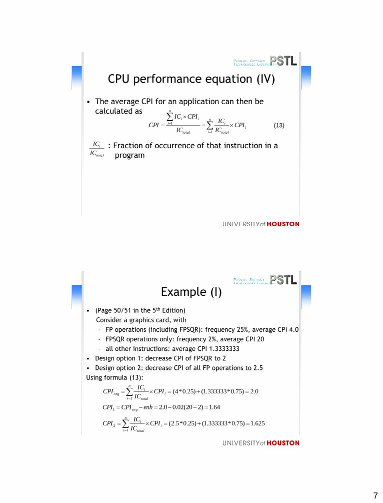
CPU performance equation (IV)

• The average CPI for an application can then be

calculated as

: Fraction of occurrence of that instruction in a

program

i

n

i total

i

total

n

i

ii

CPIIC

IC

IC

CPIIC

CPI

1

1

total

i

IC

IC

(13)

Example (I)

• (Page 50/51 in the 5th Edition)

Consider a graphics card, with

– FP operations (including FPSQR): frequency 25%, average CPI 4.0

– FPSQR operations only: frequency 2%, average CPI 20

– all other instructions: average CPI 1.3333333

• Design option 1: decrease CPI of FPSQR to 2

• Design option 2: decrease CPI of all FP operations to 2.5

Using formula (13):

64.1)220(02.00.21 enhCPICPI org

0.2)75.0*333333.1()25.0*4(1

i

n

i total

iorg CPI

IC

ICCPI

625.1)75.0*333333.1()25.0*5.2(1

2

i

n

i total

i CPIIC

ICCPI

8

Example (II)

• Slightly modified compared to the previous section:

consider a graphics card, with

– FP operations (excluding FPSQR): frequency 25%, average CPI 4.0

– FPSQR operations: frequency 2%, average CPI 20

– all other instructions: average CPI 1.33

• Design option 1: decrease CPI of FPSQR to 2

• Design option 2: decrease CPI of all FP operations to 2.5

Using formula (13):

0109.2)73.0*33.1()02.0*2()25.0*4(1

1

i

n

i total

i CPIIC

ICCPI

3709.2)73.0*33.1()02.0*20()25.0*4(1

i

n

i total

iorg CPI

IC

ICCPI

9959.1)73.0*33.1()02.0*20()25.0*5.2(1

2

i

n

i total

i CPIIC

ICCPI

Dependability

• Module reliability measures

– MTTF: mean time to failure

– FIT: failures in time

• Often expressed as failures in 1,000,000,000 hours

– MTTR: mean time to repair

– MTBF: mean time between failures

• Module availability:

MTTRMTTF

MTTFM A

MTTRMTTFMTBF

(14)

(15)

MTTFFIT

1

(16)

9

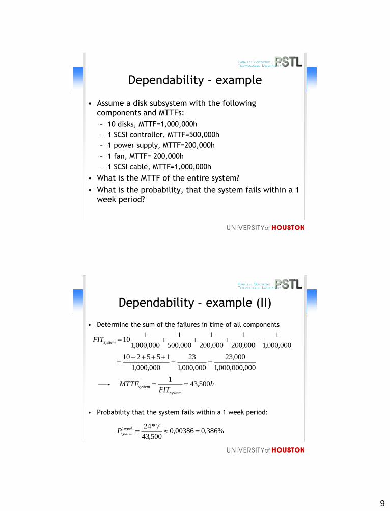
Dependability - example

• Assume a disk subsystem with the following

components and MTTFs:

– 10 disks, MTTF=1,000,000h

– 1 SCSI controller, MTTF=500,000h

– 1 power supply, MTTF=200,000h

– 1 fan, MTTF= 200,000h

– 1 SCSI cable, MTTF=1,000,000h

• What is the MTTF of the entire system?

• What is the probability, that the system fails within a 1

week period?

Dependability – example (II)

• Determine the sum of the failures in time of all components

• Probability that the system fails within a 1 week period:

000,000,1

1

000,200

1

000,200

1

000,500

1

000,000,1

110 systemFIT

000,000,000,1

000,23

000,000,1

23

000,000,1

155210

hFIT

MTTFsystem

system 500,431

%386,000386,0500,43

7*241 week

systemP

10

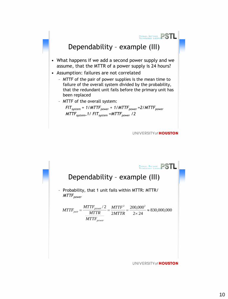
Dependability – example (III)

• What happens if we add a second power supply and we

assume, that the MTTR of a power supply is 24 hours?

• Assumption: failures are not correlated

– MTTF of the pair of power supplies is the mean time to

failure of the overall system divided by the probability,

that the redundant unit fails before the primary unit has

been replaced

– MTTF of the overall system:

FITsystem = 1/MTTFpower + 1/MTTFpower =2/MTTFpower

MTTFsystem=1/ FITsystem =MTTFpower /2

Dependability – example (III)

– Probability, that 1 unit fails within MTTR: MTTR/

MTTFpower

000,000,830242

000,200

2

2/ 22

MTTR

MTTF

MTTF

MTTR

MTTFMTTF

power

power

pair

11

Dependability – example (III)

• More generally, if

– power supply 1 has an MTTF of MTTFpower_1

– power supply 2 has an MTTF of MTTFpower_2

FITsystem = 1/MTTFpower_1 + 1/MTTFpower_2

MTTFsystem=1/ FITsystem

MTTFpair = MTTFsystem/(MTTR/min(MTTFpower_1, MTTFpower_2))

Or if either power_1 or power_2 have been clearly declared

to be the backup unit

MTTFpair = MTTFsystem/(MTTR/MTTFpower_backup)

From 1st quiz five years ago

• In order to minimize the MTTF of their mission critical computers, each

program on the space shuttle is executed by two computers

simultaneously. Computer A is from manufacturer X and has a MTTF of

40,000 hours, while computer B is from manufacturer Y and has a

different MTTF. The overall MTTF of the system is 4,000,000 hours.

– How large is the probability that the entire system (i.e. both

computers) fails during a 400 hour mission?

– What MTTF does the second/backup computer have if the MTTF of the

overall system is 4,000,000 hours, assuming that Computer A is failing

right at the beginning of the 400 hour mission and the MTTR is 400h

(i.e. the system can only be repaired after landing)?

• Solution will be posted on the web, but try first on your own!

12

Choosing the right programs to test a

system

• Most systems host a wide variety of different applications

• Profiles of certain systems given by their purpose/function

– Web server:

• high I/O requirements

• hardly any floating point operations

– A system used for weather forecasting simulations

• Very high floating point performance required

• Lots of main memory

• Number of processors have to match the problem size

calculated in order to deliver at least real-time results

Choosing the right programs to test a

system (II)

• Real application: use the target application for the

machine in order to evaluate its performance

– Best solution if application available

• Modified applications: real application has been

modified in order to measure a certain feature.

– E.g. remove I/O parts of an application in order to focus

on the CPU performance

• Application kernels: focus on the most time-consuming

parts of an application

– E.g. extract the matrix-vector multiply of an application,

since this uses 80% of the user CPU time.

13

Choosing the right programs to test a

system (III)

• Toy benchmarks: very small code segments which

produce a predictable result

– E.g. sieve of Eratosthenes, quicksort

• Synthetic benchmarks: try to match the average

frequency of operations and operands for a certain

program

– Code does not do any useful work

SPEC Benchmarks

Slides based on a talk and courtesy of

Matthias Mueller,

Center for Information Services and High Performance Computing (ZIH)

Technical University Dresden

14

What is SPEC?

•The Standard Performance Evaluation Corporation

(SPEC) is a non-profit corporation formed to establish,

maintain and endorse a standardized set of relevant

benchmarks that can be applied to the newest generation

of high-performance computers. SPEC develops suites of

benchmarks and also reviews and publishes submitted

results from our member organizations and other

benchmark licensees.

•For more details see http://www.spec.org

SPEC groups – Open Systems Group (desktop systems, high-end workstations and servers)

• CPU (CPU benchmarks)

• JAVA (java client and server side benchmarks)

• MAIL (mail server benchmarks)

• SFS (file server benchmarks)

• WEB (web server benchmarks)

– High Performance Group (HPC systems)

• OMP (OpenMP benchmark)

• HPC (HPC application benchmark)

• MPI (MPI application benchmark)

– Graphics Performance Groups (Graphics)

• Apc (Graphics application benchmarks)

• Opc (OpenGL performance benchmarks)

15

Why do we need benchmarks?

• Identify problems: measure machine properties

• Time evolution: verify that we make progress

• Coverage: help vendors to have representative codes

– Increase competition by transparency

– Drive future development (see SPEC CPU2000)

• Relevance: help customers to choose the right

computer

SPEC-Benchmarks

• All SPEC benchmarks are publicly available and well

known/understood

– Compiler can introduce special optimizations for these

benchmarks, which might be irrelevant for other, real-world

applications.

user has to provide the precise list of compile-flags

user has to provide performance of base (non-optimized) run

– Compiler can use statistical informations collected during the

first execution in order to optimize further runs (Cache hit

rates, usage of registers)

• Benchmarks designed such that external influences are kept

at a minumum (e.g. input/output)

16

SPEC CPU2000

• 26 independent programs:

– CINT2000 - integer benchmark: 12 applications (11 in C and 1 in

C++)

– CFP2000 - floating-point benchmark: 14 applications (6 in

Fortran-77, 4 in Fortran-90 and 4 in C)

• Additional information is available for each benchmark:

– Author of the benchmark

– Detailled description

– Dokumentation regarding Input and Output

– Potential problems and references.

CINT2000

17

CFP2000

Example for a CINT benchmark

18

Performance metrics • Two fundamentally different metrics:

– speed

– rate (throughput)

• For each metric results for two different optimization level have to be provided

– moderate optimization

– aggressive optimization

4 results for CINT2000 + 4 results for CFP2000 = 8 metrics

• If taking the measurements of each application individually into account:

2*2*(14+12)=104 metrics

19

Performance metrics (II) • All results are relative to a reference system

• The final results is computed by using the geometric mean values

– Speed:

– Rate:

with:

– n: number of benchmarks in a suite

– : execution time for benchmark i on the reference/test

system

– N: Number of simultaneous tasks

n

n

i runi

refi

fpt

tSPEC

1

int/ )100*(

n

n

i runi

refi

fp Nt

tSPEC

1

int/ )*16.1*(

runi

refi tt /

Reporting results • SPEC produces a minimal set of representative numbers:

+ Reducies complexity to understand correlations

+ Easies comparison of different systems

- Loss of information

• Results have to be compliant to the SPEC benchmakring rules in order to be approved as an official SPEC report

– All components have to available at least 3 month after the publication (including a runtime environment for C/C++/Fortran applications)

– Usage of SPEC tools for compiling and reporting

– Each individual benchmark has to be executed at least three times

– Verification of the benchmark output

– A maximum of four optimization flags are allowed for the base run (including preprocessor and link directives)

– Disclosure report containing all relevant data has to be available

20