Correspondences between plants and soil/environmental factors in beech forests of Central Apennines: from homogeneity to complexity

Correspondences between plants and soil/environmentalfactors in beech forests of Central Apennines:from homogeneity to complexity

Anna Testi Æ Cristina De Nicola Æ Giuseppina Dowgiallo ÆGiuliano Fanelli

Received: 28 April 2009 / Accepted: 20 August 2009� Springer-Verlag Italia 2009

Abstract Data have been collected in beech forests of central Apennines through 94

phytosociological releves and 37 soil profiles. The main edaphic factors have been ana-

lyzed. Environmental factors [light (L), temperature (T), continentality (K), soil moisture

(F), reaction (R), nitrogen (N), hemeroby (H)] have been expressed by Ellenberg bioin-

dication model and hemeroby index to estimate anthropogenic disturbance. Significant

correlations have been found by Pearson correlation test: the distribution of beech forest

typical species, such as Cephalanthera damasonium, Aquilegia vulgaris were positively

correlated with carbon/nitrogen (C/N) ratio. Five factors (T and L indicator values,

hemeroby index, CaCO3, C/N ratio) explained almost the whole variability of data set in

the canonical correspondence analysis. The relationships found between soil/environ-

mental factors and species/communities allow to detect significant differences within an

homogeneous habitat providing management indications at fine-scale.

Keywords Beech forest � Plant distribution � Soil � Hemeroby � Ellenberg indicators �Correlation � Canonical correspondence analysis

1 Introduction

It is well known that forest species are highly correlated with environmental factors

(Bocker et al. 1983; Kaiser and Kading 2005; Schaffers and Sykora 2000; Southall et al.

2004; Schmidtlein and Ewald 2003). The challenge in plant ecology is to select a reduced

set among the innumerable factors that are implied in the response of species and com-

munities. In other words, among the manifold of factors, only a few act as key factors,

structuring the ecology of communities (Fanelli et al. 2006a).

A. Testi (&) � C. De Nicola � G. Dowgiallo � G. FanelliDepartment of Plant Biology, Botanical Garden,University of Rome ‘‘La Sapienza’’, Largo Cristina di Svezia, 24,00165 Rome, Italye-mail: [email protected]

123

Rend. Fis. Acc. LinceiDOI 10.1007/s12210-009-0054-8

In ecosystems, two sets of factors are responsible for the distribution of species and

communities: static and dynamic. pH, sand, silt, clay, organic matter, pool of nitrogen in

soil, are examples of the former; mineralization rate, water input and outputs from the

ecosystem, average temperature in the course of the year, are examples of the latter. We

studied in particular static edaphic factors by soil profiles and pedological analyses.

Dynamic factors can be measured only with difficulty (Schimel and Bennet 2004) and with

long-term research effort. These factors are instead easily estimated by use of ecoindica-

tors, such as Ellenberg’s (Ellenberg 1974–1979; Testi et al. 2006a; Diekmann 1995) and

Hemeroby (Kowarik 1990) models.

Studies relating the distribution of species to environmental factors have a long history in

Central Europe; such studies are instead scarce in the Mediterranean area and in particular in

the Apennines, notwithstanding the extensive phytosociological literature. For instance,

Apennine beech woodlands are well known from a phytosociological point of view (e.g.

Feoli and Lagonegro 1982; Pignatti 1998), whereas synecological investigations are lacking.

Aims of this study are:

1. To verify the relationships between single species and soil factors in beech woodlands

of Central Apennines on calcareous rocks;

2. To study the response of the communities to the different soil and environmental

(static and dynamic) factors.

2 Materials and methods

2.1 Study area

The study was carried out within a project Life 04NAT/IT/000190 by the Department of

Plant Biology of the University of Rome (La Sapienza) and the National Forest Service.

The beech forests investigated are located in the Upper Sangro Valley in Central Apen-

nines (Abruzzo region) and include seven sites of community importance (SCI), extended

over an area of 200 km2, with altitudes ranging between 900 and 1,994 m a.s.l. This area

has a long history of silvicultural management, as in most Apennine areas: overgrazing and

fires caused a degradation of this habitat leading to soil thinning as well as to decreasing of

species diversity in the herbaceous layer. For the last 30 years silvicultural management

changed towards an ecosystemic approach: shrubs, herbs, faunistic and microbiological

components are taken into account. The managers stop to consider the forest only as an

high-productivity system, but a naturalistic management promotes the development of

stands with different stages of growth instead of coppiced stands.

The forest is dominated by Fagus sylvatica with a few specimens of Fraxinus excelsior,

Carpinus betulus, Acer campestre and Quercus robur. Occurrences of Taxus baccata and

Ilex aquifolium were recorded in mixed stands with Fagus according to ‘‘European Habitat

Directive 2000’’.

Although the beech stands are rather homogeneous in the composition of the herbaceous

layer, they show differences both in the density and in the species richness of the under-

story: a mosaic-like pattern of species-poor stands with low coverage alternated with richer

stands with clonal populations of Cardamine enneaphyllos, Cardamine bulbifera, Galiumodoratum, Viola reichenbachiana, Corydalis cava.

The main bedrocks in the area are calcareous. Most of the soils found throughout the

study area (De Nicola et al. 2007a) have a moderately deep ABwC profile: they consist of a

Rend. Fis. Acc. Lincei

123

rather thin epipedon with a crumb structure, brownish black colors and very high organic

matter contents (from 10 up to 20%) and a cambic B horizon, subangular blocky, often

containing calcareous gravel and gradually merging into a stony C horizon. Most of these

soils are slightly acid to neutral and free of primary carbonates, but have a rather high base

saturation ([60%), thus they can be classified as Dystric Eutrudepts. Occasionally Typical

Eutrudepts have been found, which are slightly to moderately alkaline throughout the

profile, slightly calcareous and with very high base contents (BS [ 90%). All these soils

are moderately fine textured (silt loam) and have a medium to very high water availability

(AWC = 120–280 mm). Their moisture regime is udic, the temperature regime ranges

from mesic to frigid with altitude.

In strongly eroded areas, the dominant soils are rendzina-types with a xeric moisture

regime (Lithic and Typic Haploxerolls) with a very dark mollic epipedon, very rich in

organic matter (16–26%), 35–50 cm thick, underlain by a stony C horizon, or, more rarely,

by hard limestone. These soils have a loamy texture with abundant calcareous fragments of

various sizes and a rather low water availability (80–100 mm); the matrix is slightly to

moderately calcareous and pH values are neutral or slightly alkaline.

2.2 Vegetation data collecting

In the first step vegetation data were collected in 94 sampling sites chosen to represent:

(1) different vegetation types;

(2) different forest management types.

Sampling sites are 100 m2 in size. In each one, vegetation composition was surveyed

with a phytosociological releve. Nomenclature of species follows Pignatti (1982).

A matrix of 175 species 9 94 releves was obtained.

2.3 Sampling design

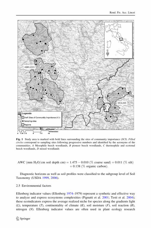
Among the 94 sampling sites, a subset of 37 plots (Fig. 1) was selected for soil profile

description and pedological analyses. These plots were chosen to represent different plant

communities and different forest management types, based on the following repartitions:

ten plots in coppiced stands, ten in the mature high-growth forest stands, ten in the young

high-growth forest stands and seven in stands under transition to high forest. Soil and

vegetation data have been collected simultaneously.

2.4 Soil factors sampling

In the subset of 37 plots, soil profiles were studied through pits and augering. For field

description of the macromorphological soil characteristics the Soil Survey Division Staff

(1993) was used. The following physical and chemical analyses were carried out on a total

of 111 soil samples, according to USDA methods (1996): pH (in H2O), total calcium

carbonate (CaCO3), particle-size analysis, organic carbon (C) and nitrogen content,

exchangeable bases (Ca??, Na?, K?, Mg??), cation exchange capacity (CEC),

exchangeable acidity (EA), base saturation (BS). Moreover, two other factors were cal-

culated: available water capacity (AWC) and ratio between carbon and nitrogen (C/N).

Available water capacity was estimated using the following equation proposed by Salter

and Williams (1969), based on textural composition and percentage of organic matter:


123

AWC ðmm H2O=cm soil depth cm) ¼ 1:475� 0:010 ð% coarse sandÞ þ 0:011 ð% siltÞþ 0:138 ð% organic carbonÞ:

Diagnostic horizons as well as soil profiles were classified to the subgroup level of Soil

Taxonomy (USDA 1999, 2006).

2.5 Environmental factors

Ellenberg indicator values (Ellenberg 1974–1979) represent a synthetic and effective way

to analyze and express ecosystems complexities (Pignatti et al. 2001; Testi et al. 2004);

these ecoindicators express the average realized niche for species along the gradients light

(L), temperature (T), continentality of climate (K), soil moisture (F), soil reaction (R),

nitrogen (N). Ellenberg indicator values are often used in plant ecology research

Fig. 1 Study area is marked with bold lines surrounding the sites of community importance (SCI). Filledcircles correspond to sampling sites following progressive numbers and identified by the acronyms of thecommunities. A Mesophile beech woodlands, B pioneer beech woodlands, C thermophile and ecotonalbeech woodlands, D mixed woodlands


123

(Diekmann 1995; Schaffers and Sykora 2000), in comparative studies on plant commu-

nities (Dupre and Diekmann 1998; Testi et al. 2006b), and to relate vegetation patterns to

environmental changes (Pignatti et al. 2001). Since the beginning of phytosociology,

Braun-Blanquet and Jenny (1926) and Guinochet (1938) pointed out that species occur-

rences and plant associations may be defined through an ecological approach based on

factors measured in the field as well as on ecological indicators (Ellenberg 1963); they

foresaw the development of a multidimensional analysis overcoming the approach

exclusively based on floristic analysis.

Closely related to Ellenberg indicator values is the Hemeroby index (H), expressing the

degree of past and present human disturbance on ecosystems according to a ten-point scale

(van der Maarel 1979; Kowarik 1990; Fanelli and De Lillis 2004). Disturbance is a general

ecological factor in nature and it is a primary cause of spatial heterogeneity in ecosystems

(Platt 1975; Loucks et al. 1985; Collins and Glenn 1988; White and Jentsch 2001).

Unfortunately, direct estimation of disturbance and human impact is usually difficult. It is

therefore necessary to evaluate disturbance indirectly by means of changes in the com-

position of communities. So, in practice we do not study disturbance directly, but the

response of vegetation to disturbance (Fanelli and Testi 2008).

The figures for ecoindicators have been taken from a data-bank for the species of the

Mediterranean flora (Fanelli et al. 2006b, c). The values were averaged over the matrix

‘‘species/releves’’, obtaining an ecological matrix where each species had seven indicators

values (L, T, K, F, R, N, H). For each plot, indicator values were weighted on the species

coverages, obtaining an ecological characterization for site.

2.6 Statistical analysis

Pearson correlation test was applied to investigate the relationships between species dis-

tribution and soil factors. Furthermore, since soil and environmental factors are indepen-

dently measured and calculated, also correlations between them were considered. In order

to identify multivariate correspondence between all analyzed soil/environmental factors

expressed by ecoindicators and coverage of all species, canonical correspondence analysis

(CCA) has been applied using SYNTAX 2000 (Podani 2000). The normalized scores for

factors stressing their weight on the CCA axes were utilized to recognize the main gra-

dients along which species and communities were distributed. The CCA results are pre-

sented as ordination triplots with sampling plots, species and soil/environmental factors by

scores for set with axes constrained.

3 Results

3.1 Vegetation

The 94 plots of the complete dataset can be grouped into four types of communities that

have been previously recognized in a separate study (De Nicola et al. 2007a); these types

are represented in a map of the study area (Fig. 1):

• mesophile beech woodlands at higher altitudes; this type is the most widespread in the

study area (Type A).

• pioneer beech woodlands, mainly distributed in the NE slope of the mountain ridges on

stony soils (Type B).


123

• thermophile beech woodlands at lower altitudes; this type is quite rare in the study area

(Type C).

• mixed woodlands with turkey oak (Quercus cerris) on marls, at lower altitudes (Type

D).

3.2 Output of correlation analysis

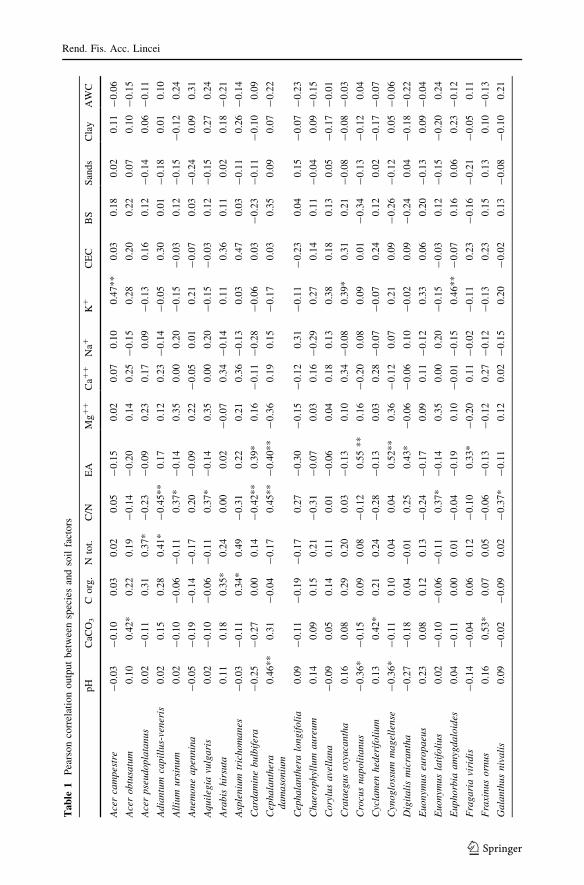
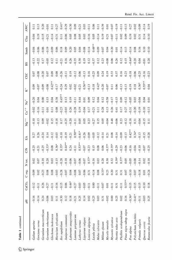
Pearson correlation test performed on the subset of 37 plots where phytosociological

releves and soil profiles were simultaneously carried out, displayed many significant

correlations between species and soil factors. Individual species resulted positively or

negatively correlated with one or more soil factors (Table 1). Furthermore, many signifi-

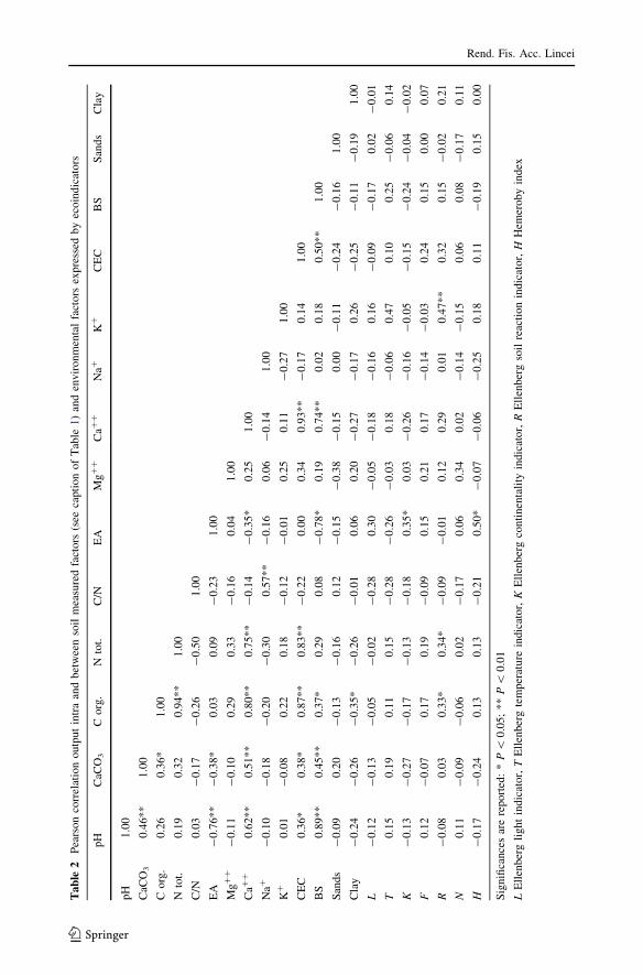
cant correlations emerged also from intra-data set and from measured soil factors versusecoindicators (Table 2).

It is worth mentioning that in many cases correlations between species and soil factors

resulted significant even when correlation coefficients were low (for instance the corre-

lation between Rhamnus alpinus and organic carbon has r2 = 0.34 but is nonetheless

significant).

The most important correlations reported in Tables 1 and 2 are described below:

CaCO3 Soils with high content of calcium carbonate are positively correlated with tree

species such as Laburnum anagyroides, Fraxinus ornus, Pinus nigra subsp. nigra and Acerobtusatum: these species colonize sites where competition with Fagus is low (Pignatti

1998). CaCO3 is also positively correlated with pH, CEC, organic carbon, BS, Ca?? and

negatively with EA.

C Organic carbon is correlated with species occurring at the edge of the forest, such as

Rhamnus alpinus subsp. fallax, Arabis hirsuta, Asplenium trichomanes, Milium effusum,

Scrophularia peregrina, exhibiting high requirement for soil nutrients (Wilson et al. 2001),

as shown by high values of nitrogen Ellenberg indicator (N), ranged between 7 and 8.

Organic carbon is also correlated with soil reaction indicator value (R) and with several soil

factors: CEC, BS, CaCO3, nitrogen content, Ca??.

Nitrogen content Several species distributed in the different communities are positively

correlated with nitrogen content. This factor is also correlated with R indicator and with

other soil factors such as organic carbon, Ca??, and CEC. Correlation values for organic

carbon, Ca?? and CEC are very high (0.75–0.83) (Table 2).

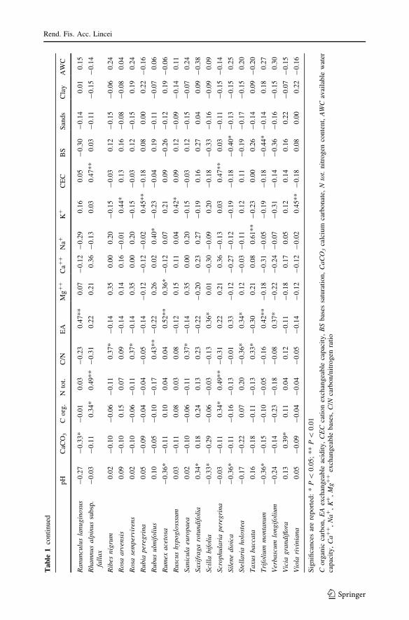
C/N ratio Carbon/nitrogen (C/N) ratio is the factor that is correlated with the largest

number of different species; these are mainly mesophile species (more common in Type A

woodlands): Taxus baccata, Cephalanthera damasonium, Ilex aquifolium, Lathyrus vernus,

Euonymus latifolius, Ribes nigrum, Sanicula europaea, Allium ursinum, Aquilegiavulgaris, Hieracium sylvaticum.

pH Correlations with pH allow to discriminate subacidophile species (Poa alpina,

Cynoglossum magellense, Crocus napolitanus, Polystichum lonchitis, Rumex acetosa,

Scilla bifolia), with negative coefficient values and basophile ones (Cephalantheradamasonium, Saxifraga rotundifolia) with positive correlation: the first are dominant in

open spaces represented by wood-clearings and pasturelands; the second occur in beech

forest.


123

Tab

le1

Pea

rson

corr

elat

ion

outp

ut

bet

wee

nsp

ecie

san

dso

ilfa

ctors

pH

CaC

O3

Co

rg.

Nto

t.C

/NE

AM

g?

?C

a??

Na?

K?

CE

CB

SS

and

sC

lay

AW

C

Ace

rca

mp

estr

e-

0.0

3-

0.1

00

.03

0.0

20

.05

-0

.15

0.0

20

.07

0.1

00

.47

**

0.0

30

.18

0.0

20

.11

-0

.06

Ace

ro

btu

satu

m0

.10

0.4

2*

0.2

20

.19

-0

.14

-0

.20

0.1

40

.25

-0

.15

0.2

80

.20

0.2

20

.07

0.1

0-

0.1

5

Ace

rp

seu

do

pla

tan

us

0.0

2-

0.1

10

.31

0.3

7*

-0

.23

-0

.09

0.2

30

.17

0.0

9-

0.1

30

.16

0.1

2-

0.1

40

.06

-0

.11

Ad

ian

tum

cap

illu

s-ve

ner

is0

.02

0.1

50

.28

0.4

1*

-0

.45

**

0.1

70

.12

0.2

3-

0.1

4-

0.0

50

.30

0.0

1-

0.1

80

.01

0.1

0

All

ium

urs

inu

m0

.02

-0

.10

-0

.06

-0

.11

0.3

7*

-0

.14

0.3

50

.00

0.2

0-

0.1

5-

0.0

30

.12

-0

.15

-0

.12

0.2

4

An

emo

ne

ap

enn

ina

-0

.05

-0

.19

-0

.14

-0

.17

0.2

0-

0.0

90

.22

-0

.05

0.0

10

.21

-0

.07

0.0

3-

0.2

40

.09

0.3

1

Aq

uil

egia

vulg

ari

s0

.02

-0

.10

-0

.06

-0

.11

0.3

7*

-0

.14

0.3

50

.00

0.2

0-

0.1

5-

0.0

30

.12

-0

.15

0.2

70

.24

Ara

bis

hir

suta

0.1

10

.18

0.3

5*

0.2

40

.00

0.0

2-

0.0

70

.34

-0

.14

0.1

10

.36

0.1

10

.02

0.1

8-

0.2

1

Asp

len

ium

tric

ho

ma

nes

-0

.03

-0

.11

0.3

4*

0.4

9-

0.3

10

.22

0.2

10

.36

-0

.13

0.0

30

.47

0.0

3-

0.1

10

.26

-0

.14

Ca

rda

min

eb

ulb

ifer

a-

0.2

5-

0.2

70

.00

0.1

4-

0.4

2*

*0

.39

*0

.16

-0

.11

-0

.28

-0

.06

0.0

3-

0.2

3-

0.1

1-

0.1

00

.09

Cep

ha

lan

ther

ad

am

aso

niu

m0

.46

**

0.3

1-

0.0

4-

0.1

70

.45

**

-0

.40

**

-0

.36

0.1

90

.15

-0

.17

0.0

30

.35

0.0

90

.07

-0

.22

Cep

ha

lan

ther

alo

ng

ifo

lia

0.0

9-

0.1

1-

0.1

9-

0.1

70

.27

-0

.30

-0

.15

-0

.12

0.3

1-

0.1

1-

0.2

30

.04

0.1

5-

0.0

7-

0.2

3

Ch

aer

op

hyl

lum

au

reu

m0

.14

0.0

90

.15

0.2

1-

0.3

1-

0.0

70

.03

0.1

6-

0.2

90

.27

0.1

40

.11

-0

.04

0.0

9-

0.1

5

Co

rylu

sa

vell

an

a-

0.0

90

.05

0.1

40

.11

0.0

1-

0.0

60

.04

0.1

80

.13

0.3

80

.18

0.1

30

.05

-0

.17

-0

.01

Cra

taeg

us

oxy

aca

nth

a0

.16

0.0

80

.29

0.2

00

.03

-0

.13

0.1

00

.34

-0

.08

0.3

9*

0.3

10

.21

-0

.08

-0

.08

-0

.03

Cro

cus

na

po

lita

nu

s-

0.3

6*

-0

.15

0.0

90

.08

-0

.12

0.5

5*

*0

.16

-0

.20

0.0

80

.09

0.0

1-

0.3

4-

0.1

3-

0.1

20

.04

Cyc

lam

enh

eder

ifo

liu

m0

.13

0.4

2*

0.2

10

.24

-0

.28

-0

.13

0.0

30

.28

-0

.07

-0

.07

0.2

40

.12

0.0

2-

0.1

7-

0.0

7

Cyn

og

loss

um

ma

gel

len

se-

0.3

6*

-0

.11

0.1

00

.04

0.0

40

.52

**

0.3

6-

0.1

20

.07

0.2

10

.09

-0

.26

-0

.12

0.0

5-

0.0

6

Dig

ita

lis

mic

ran

tha

-0

.27

-0

.18

0.0

4-

0.0

10

.25

0.4

3*

-0

.06

-0

.06

0.1

0-

0.0

20

.09

-0

.24

0.0

4-

0.1

8-

0.2

2

Eu

on

ymu

seu

rop

aeu

s0

.23

0.0

80

.12

0.1

3-

0.2

4-

0.1

70

.09

0.1

1-

0.1

20

.33

0.0

60

.20

-0

.13

0.0

9-

0.0

4

Eu

on

ymu

sla

tifo

liu

s0

.02

-0

.10

-0

.06

-0

.11

0.3

7*

-0

.14

0.3

50

.00

0.2

0-

0.1

5-

0.0

30

.12

-0

.15

-0

.20

0.2

4

Eu

ph

orb

iaa

myg

da

loid

es0

.04

-0

.11

0.0

00

.01

-0

.04

-0

.19

0.1

0-

0.0

1-

0.1

50

.46

**

-0

.07

0.1

60

.06

0.2

3-

0.1

2

Fra

ga

ria

viri

dis

-0

.14

-0

.04

0.0

60

.12

-0

.10

0.3

3*

-0

.20

0.1

1-

0.0

2-

0.1

10

.23

-0

.16

-0

.21

-0

.05

0.1

1

Fra

xin

us

orn

us

0.1

60

.53

*0

.07

0.0

5-

0.0

6-

0.1

3-

0.1

20

.27

-0

.12

-0

.13

0.2

30

.15

0.1

30

.10

-0

.13

Ga

lan

thu

sn

iva

lis

0.0

9-

0.0

2-

0.0

90

.02

-0

.37

*-

0.1

10

.12

0.0

2-

0.1

50

.20

-0

.02

0.1

3-

0.0

8-

0.1

00

.21


123

Tab

le1

con

tin

ued

pH

CaC

O3

Co

rg.

Nto

t.C

/NE

AM

g?

?C

a??

Na?

K?

CE

CB

SS

and

sC

lay

AW

C

Ga

liu

ma

pa

rin

e-

0.1

6-

0.1

2-

0.0

90

.02

-0

.25

0.2

7-

0.1

0-

0.0

2-

0.2

00

.09

0.0

7-

0.1

3-

0.0

4-

0.0

40

.11

Gen

zia

na

vern

a-

0.1

4-

0.1

10

.02

0.0

7-

0.2

10

.26

-0

.13

-0

.16

0.0

4-

0.0

7-

0.0

8-

0.2

2-

0.0

60

.19

0.1

3

Ger

an

ium

ma

cro

rrh

izu

m0

.24

0.2

6-

0.2

3-

0.1

8-

0.2

5-

0.2

40

.09

-0

.11

0.0

0-

0.0

9-

0.2

00

.17

-0

.06

-0

.15

0.2

0

Ger

an

ium

rob

erti

an

um

-0

.06

-0

.27

0.0

80

.20

-0

.33

*0

.14

-0

.02

0.0

10

.15

-0

.08

0.0

7-

0.0

5-

0.1

9-

0.2

1-

0.0

1

Gle

cho

ma

hed

era

cea

0.0

3-

0.1

10

.08

0.0

30

.08

-0

.12

0.1

50

.11

0.0

40

.42

**

0.0

90

.12

-0

.09

-0

.14

0.1

1

Hie

raci

um

sylv

ati

cum

0.1

1-

0.1

6-

0.0

3-

0.1

50

.36

*-

0.0

3-

0.1

80

.08

0.3

8-

0.1

70

.08

0.1

10

.06

-0

.31

-0

.27

Ilex

aq

uif

oli

um

-0

.30

-0

.15

-0

.28

-0

.28

0.3

5*

-0

.10

0.1

7-

0.2

30

.45

**

-0

.24

-0

.26

-0

.21

0.1

80

.11

0.4

1*

Jun

iper

us

com

mu

nis

0.1

20

.06

-0

.07

-0

.18

0.4

4*

*-

0.1

9-

0.2

5-

0.0

30

.13

0.2

9-

0.1

10

.16

0.0

9-

0.0

6-

0.2

9

La

bu

rnu

ma

na

gyr

oid

es0

.18

0.4

4*

0.0

4-

0.0

60

.24

-0

.21

-0

.20

0.2

60

.19

0.0

20

.19

0.2

60

.20

0.0

5-

0.3

0

La

miu

mg

arg

an

icu

m-

0.2

1-

0.2

7-

0.0

8-

0.0

7-

0.1

10

.50

**

-0

.11

-0

.28

-0

.11

-0

.02

-0

.12

-0

.35

0.0

50

.08

0.0

9

La

thyr

us

vern

us

0.2

5-

0.0

30

.07

-0

.06

0.5

3*

*-

0.4

1*

0.0

50

.19

0.4

4-

0.2

10

.06

0.3

00

.04

0.0

5-

0.2

1

Lig

ust

rum

vulg

are

0.1

4-

0.0

5-

0.0

6-

0.0

7-

0.0

7-

0.2

60

.05

-0

.04

0.0

10

.56

**

-0

.13

0.1

9-

0.0

80

.03

0.0

3

Lo

nic

era

alp

igen

a0

.02

-0

.11

0.3

10

.37

*-

0.2

3-

0.0

90

.23

0.1

70

.09

-0

.13

0.1

60

.12

-0

.14

-0

.16

-0

.11

Lu

zula

pil

osa

-0

.25

0.0

0-

0.1

4-

0.1

60

.15

-0

.05

-0

.27

-0

.21

0.1

2-

0.1

8-

0.2

5-

0.3

70

.48

**

0.0

50

.06

Ma

lus

sylv

estr

is0

.03

-0

.11

0.0

80

.03

0.0

8-

0.1

20

.15

0.1

10

.04

0.4

2*

0.0

90

.12

-0

.09

-0

.14

0.1

1

Mil

ium

efu

sum

0.3

1-

0.0

70

.33

*0

.28

0.0

6-

0.1

40

.05

0.2

80

.12

-0

.20

0.2

40

.23

-0

.07

0.1

9-

0.3

9

Myc

elis

mu

rali

s-

0.0

20

.01

0.2

30

.30

-0

.37

*0

.21

-0

.04

0.1

3-

0.5

8-

0.0

70

.19

-0

.08

0.0

40

.21

0.0

1

Myo

soti

ssy

lva

tica

0.0

0-

0.1

10

.20

0.3

2-

0.3

5*

0.0

80

.48

0.2

6-

0.1

70

.11

0.3

30

.06

-0

.20

-0

.07

-0

.07

Neo

ttia

nid

us

avi

s0

.25

0.3

10

.31

0.3

9*

-0

.29

-0

.14

-0

.06

0.4

1-

0.1

50

.06

0.3

70

.26

0.0

1-

0.1

1-

0.1

9

Ph

ylli

tis

sco

lop

end

riu

m0

.02

-0

.11

0.3

10

.37

*-

0.2

3-

0.0

90

.23

0.1

70

.09

-0

.13

0.1

60

.12

-0

.14

0.0

2-

0.1

1

Pin

us

nig

rasu

bsp

.n

igra

0.1

60

.53

**

0.0

70

.05

-0

.06

-0

.13

-0

.12

0.2

7-

0.1

2-

0.1

30

.23

0.1

50

.13

0.0

9-

0.1

3

Po

aa

lpin

a-

0.3

6*

-0

.15

-0

.10

-0

.05

-0

.16

0.4

2*

*-

0.1

8-

0.3

1-

0.0

5-

0.1

9-

0.1

8-

0.4

4*

-0

.14

0.1

90

.27

Po

lyst

ich

um

lon

chit

is-

0.4

1*

-0

.15

-0

.07

-0

.08

-0

.04

0.3

4*

0.3

1-

0.2

00

.03

0.1

8-

0.0

6-

0.2

00

.08

0.0

2-

0.0

2

Pri

mu

lavu

lga

ris

-0

.11

-0

.15

-0

.18

-0

.14

-0

.10

-0

.13

-0

.04

-0

.19

-0

.04

0.3

6*

-0

.25

0.0

40

.16

0.3

1-

0.0

9

Qu

ercu

sce

rris

-0

.03

-0

.10

0.0

10

.02

-0

.07

-0

.15

-0

.15

-0

.10

0.0

40

.55

**

-0

.16

-0

.01

0.1

00

.14

-0

.14

Ra

nu

ncu

lus

fica

ria

0.2

50

.18

-0

.24

-0

.18

-0

.25

-0

.28

0.1

1-

0.1

30

.01

0.0

4-

0.2

30

.20

-0

.10

-0

.10

0.1

9


123

Tab

le1

con

tin

ued

pH

CaC

O3

Co

rg.

Nto

t.C

/NE

AM

g?

?C

a??

Na?

K?

CE

CB

SS

and

sC

lay

AW

C

Ra

nu

ncu

lus

lan

ug

ino

sus

-0

.27

-0

.33

*-

0.0

10

.03

-0

.23

0.4

7*

*0

.07

-0

.12

-0

.29

0.1

60

.05

-0

.30

-0

.14

0.0

10

.15

Rh

am

nu

sa

lpin

us

sub

sp.

fall

ax

-0

.03

-0

.11

0.3

4*

0.4

9*

*-

0.3

10

.22

0.2

10

.36

-0

.13

0.0

30

.47

**

0.0

3-

0.1

1-

0.1

5-

0.1

4

Rib

esn

igru

m0

.02

-0

.10

-0

.06

-0

.11

0.3

7*

-0

.14

0.3

50

.00

0.2

0-

0.1

5-

0.0

30

.12

-0

.15

-0

.06

0.2

4

Ro

saa

rven

sis

0.0

9-

0.1

00

.15

0.0

70

.09

-0

.14

0.1

40

.16

-0

.01

0.4

4*

0.1

30

.16

-0

.08

-0

.08

0.0

4

Ro

sase

mp

ervi

ren

s0

.02

-0

.10

-0

.06

-0

.11

0.3

7*

-0

.14

0.3

50

.00

0.2

0-

0.1

5-

0.0

30

.12

-0

.15

0.1

90

.24

Ru

bia

per

egri

na

0.0

5-

0.0

9-

0.0

4-

0.0

4-

0.0

5-

0.1

4-

0.1

2-

0.1

2-

0.0

20

.45

**

-0

.18

0.0

80

.00

0.2

2-

0.1

6

Ru

bu

su

lmif

oli

us

0.1

0-

0.0

5-

0.1

0-

0.1

70

.43

**

-0

.22

0.2

60

.02

0.4

0*

-0

.23

-0

.04

0.1

9-

0.1

1-

0.0

70

.06

Ru

mex

ace

tosa

-0

.36

*-

0.1

10

.10

0.0

40

.04

0.5

2*

*0

.36

*-

0.1

20

.07

0.2

10

.09

-0

.26

-0

.12

0.1

9-

0.0

6

Ru

scu

sh

ypo

glo

sssu

m0

.03

-0

.11

0.0

80

.03

0.0

8-

0.1

20

.15

0.1

10

.04

0.4

2*

0.0

90

.12

-0

.09

-0

.14

0.1

1

Sa

nic

ula

euro

pa

ea0

.02

-0

.10

-0

.06

-0

.11

0.3

7*

-0

.14

0.3

50

.00

0.2

0-

0.1

5-

0.0

30

.12

-0

.15

-0

.07

0.2

4

Sa

xifr

ag

aro

tun

dif

oli

a0

.34

*0

.18

0.2

40

.13

0.2

3-

0.2

2-

0.2

00

.23

0.2

7-

0.1

90

.16

0.2

70

.04

0.0

9-

0.3

8

Sci

lla

bif

oli

a-

0.3

3*

-0

.29

-0

.06

-0

.03

-0

.13

0.3

6*

0.0

1-

0.3

0-

0.0

90

.20

-0

.18

-0

.33

-0

.16

-0

.09

0.0

9

Scr

op

hu

lari

ap

ereg

rin

a-

0.0

3-

0.1

10

.34

*0

.49

**

-0

.31

0.2

20

.21

0.3

6-

0.1

30

.03

0.4

7*

*0

.03

-0

.11

-0

.15

-0

.14

Sil

ene

dio

ica

-0

.36

*-

0.1

1-

0.1

6-

0.1

3-

0.0

10

.33

-0

.12

-0

.27

-0

.12

-0

.19

-0

.18

-0

.40

*-

0.1

3-

0.1

50

.25

Ste

lla

ria

ho

lost

ea-

0.1

7-

0.2

20

.07

0.2

0-

0.3

6*

0.3

4*

0.1

2-

0.0

3-

0.1

10

.12

0.1

1-

0.1

9-

0.1

7-

0.1

50

.20

Ta

xus

ba

cca

ta0

.16

-0

.18

-0

.11

-0

.13

0.3

3*

-0

.30

0.2

10

.08

0.6

1*

*-

0.2

30

.00

0.2

6-

0.1

40

.09

-0

.20

Tri

foli

um

mo

nta

nu

m-

0.3

6*

-0

.15

-0

.10

-0

.05

-0

.16

0.4

2*

*-

0.1

8-

0.3

1-

0.0

5-

0.1

9-

0.1

8-

0.4

4*

-0

.14

0.1

80

.27

Ver

ba

scu

mlo

ng

ifo

liu

m-

0.2

4-

0.1

4-

0.2

3-

0.1

8-

0.0

80

.37

*-

0.2

2-

0.2

4-

0.0

7-

0.3

1-

0.1

4-

0.3

6-

0.1

6-

0.1

50

.30

Vic

iag

ran

difl

ora

0.1

30

.39

*0

.11

0.0

40

.12

-0

.11

-0

.18

0.1

70

.05

0.1

20

.14

0.1

60

.22

-0

.07

-0

.15

Vio

lari

vin

ian

a0

.05

-0

.09

-0

.04

-0

.04

-0

.05

-0

.14

-0

.12

-0

.12

-0

.02

0.4

5*

*-

0.1

80

.08

0.0

00

.22

-0

.16

Sig

nifi

can

ces

are

rep

ort

ed:

*P

\0

.05

;*

*P

\0

.01

Co

rgan

icca

rbo

n,

EA

exch

ang

eab

leac

idit

y,

CE

Cca

tio

nex

chan

gea

ble

cap

acit

y,

BS

bas

essa

tura

tio

n,

Ca

CO

3ca

lciu

mca

rbo

nat

e,N

tot.

nit

rog

enco

nte

nt,

AW

Cav

aila

ble

wat

erca

pac

ity

,C

a?

?,

Na

?,

K?

,M

g?

?ex

chan

gea

ble

bas

es,

C/N

carb

on

/nit

rog

enra

tio


123

Ta

ble

2P

ears

on

corr

elat

ion

ou

tpu

tin

tra

and

bet

wee

nso

ilm

easu

red

fact

ors

(see

capti

on

of

Tab

le1)

and

env

iro

nm

enta

lfa

cto

rsex

pre

ssed

by

eco

ind

icat

ors

pH

CaC

O3

Co

rg.

Nto

t.C

/NE

AM

g?

?C

a??

Na?

K?

CE

CB

SS

and

sC

lay

pH

1.0

0

CaC

O3

0.4

6*

*1

.00

Co

rg.

0.2

60

.36*

1.0

0

Nto

t.0

.19

0.3

20

.94*

*1

.00

C/N

0.0

3-

0.1

7-

0.2

6-

0.5

01

.00

EA

-0

.76*

*-

0.3

8*

0.0

30

.09

-0

.23

1.0

0

Mg

??

-0

.11

-0

.10

0.2

90

.33

-0

.16

0.0

41

.00

Ca?

?0

.62*

*0

.51*

*0

.80*

*0

.75

**

-0

.14

-0

.35*

0.2

51

.00

Na?

-0

.10

-0

.18

-0

.20

-0

.30

0.5

7*

*-

0.1

60

.06

-0

.14

1.0

0

K?

0.0

1-

0.0

80

.22

0.1

8-

0.1

2-

0.0

10

.25

0.1

1-

0.2

71

.00

CE

C0

.36*

0.3

8*

0.8

7*

*0

.83

**

-0

.22

0.0

00

.34

0.9

3*

*-

0.1

70

.14

1.0

0

BS

0.8

9*

*0

.45*

*0

.37*

0.2

90

.08

-0

.78*

0.1

90

.74*

*0

.02

0.1

80

.50*

*1

.00

San

ds

-0

.09

0.2

0-

0.1

3-

0.1

60

.12

-0

.15

-0

.38

-0

.15

0.0

0-

0.1

1-

0.2

4-

0.1

61

.00

Cla

y-

0.2

4-

0.2

6-

0.3

5*

-0

.26

-0

.01

0.0

60

.20

-0

.27

-0

.17

0.2

6-

0.2

5-

0.1

1-

0.1

91

.00

L-

0.1

2-

0.1

3-

0.0

5-

0.0

2-

0.2

80

.30

-0

.05

-0

.18

-0

.16

0.1

6-

0.0

9-

0.1

70

.02

-0

.01

T0

.15

0.1

90

.11

0.1

5-

0.2

8-

0.2

6-

0.0

30

.18

-0

.06

0.4

70

.10

0.2

5-

0.0

60

.14

K-

0.1

3-

0.2

7-

0.1

7-

0.1

3-

0.1

80

.35*

0.0

3-

0.2

6-

0.1

6-

0.0

5-

0.1

5-

0.2

4-

0.0

4-

0.0

2

F0

.12

-0

.07

0.1

70

.19

-0

.09

0.1

50

.21

0.1

7-

0.1

4-

0.0

30

.24

0.1

50

.00

0.0

7

R-

0.0

80

.03

0.3

3*

0.3

4*

-0

.09

-0

.01

0.1

20

.29

0.0

10

.47

**

0.3

20

.15

-0

.02

0.2

1

N0

.11

-0

.09

-0

.06

0.0

2-

0.1

70

.06

0.3

40

.02

-0

.14

-0

.15

0.0

60

.08

-0

.17

0.1

1

H-

0.1

7-

0.2

40

.13

0.1

3-

0.2

10

.50*

-0

.07

-0

.06

-0

.25

0.1

80

.11

-0

.19

0.1

50

.00

Sig

nifi

cance

sar

ere

port

ed:

*P

\0

.05;

**

P\

0.0

1

LE

llen

ber

gli

gh

tin

dic

ato

r,T

Ell

enber

gte

mp

erat

ure

indic

ato

r,K

Ell

enb

erg

con

tin

enta

lity

ind

icat

or,

RE

llen

ber

gso

ilre

acti

on

indic

ator,

HH

emer

oby

ind

ex


123

K? Potassium shows positive correlations only with species such as Quercus cerris, Acercampestre, Ligustrum vulgare, Euphorbia amygdaloides, Rubia peregrina, species typical

of mixed woodlands.

Soil exchangeable acidity EA is positively correlated with species prevailing on the

forest fringes and wood clearings (Digitalis micrantha, Cynoglossum magellense, Fragariaviridis, Lamium garganicum, Ranunculus lanuginosus, Stellaria holostea, Trifoliummontanum, Verbascum longifolium). This soil factor is correlated positively with hemeroby

index (H), continentality indicator (K), and negatively with BS and Ca??.

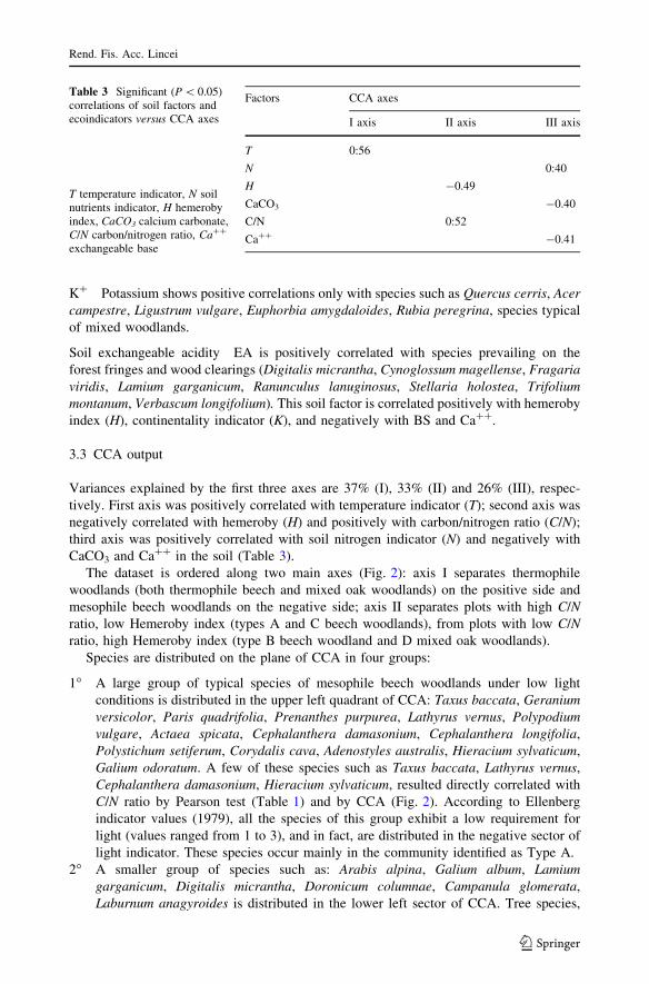
3.3 CCA output

Variances explained by the first three axes are 37% (I), 33% (II) and 26% (III), respec-

tively. First axis was positively correlated with temperature indicator (T); second axis was

negatively correlated with hemeroby (H) and positively with carbon/nitrogen ratio (C/N);

third axis was positively correlated with soil nitrogen indicator (N) and negatively with

CaCO3 and Ca?? in the soil (Table 3).

The dataset is ordered along two main axes (Fig. 2): axis I separates thermophile

woodlands (both thermophile beech and mixed oak woodlands) on the positive side and

mesophile beech woodlands on the negative side; axis II separates plots with high C/Nratio, low Hemeroby index (types A and C beech woodlands), from plots with low C/Nratio, high Hemeroby index (type B beech woodland and D mixed oak woodlands).

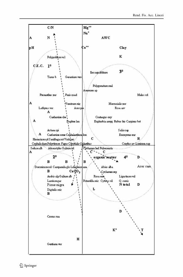
Species are distributed on the plane of CCA in four groups:

1� A large group of typical species of mesophile beech woodlands under low light

conditions is distributed in the upper left quadrant of CCA: Taxus baccata, Geraniumversicolor, Paris quadrifolia, Prenanthes purpurea, Lathyrus vernus, Polypodiumvulgare, Actaea spicata, Cephalanthera damasonium, Cephalanthera longifolia,

Polystichum setiferum, Corydalis cava, Adenostyles australis, Hieracium sylvaticum,

Galium odoratum. A few of these species such as Taxus baccata, Lathyrus vernus,

Cephalanthera damasonium, Hieracium sylvaticum, resulted directly correlated with

C/N ratio by Pearson test (Table 1) and by CCA (Fig. 2). According to Ellenberg

indicator values (1979), all the species of this group exhibit a low requirement for

light (values ranged from 1 to 3), and in fact, are distributed in the negative sector of

light indicator. These species occur mainly in the community identified as Type A.

2� A smaller group of species such as: Arabis alpina, Galium album, Lamiumgarganicum, Digitalis micrantha, Doronicum columnae, Campanula glomerata,

Laburnum anagyroides is distributed in the lower left sector of CCA. Tree species,

Table 3 Significant (P \ 0.05)correlations of soil factors andecoindicators versus CCA axes

T temperature indicator, N soilnutrients indicator, H hemerobyindex, CaCO3 calcium carbonate,C/N carbon/nitrogen ratio, Ca??

exchangeable base

Factors CCA axes

I axis II axis III axis

T 0:56

N 0:40

H -0.49

CaCO3 -0.40

C/N 0:52

Ca?? -0.41


123


123

such as Laburnum anagyroides and Pinus nigra subsp. nigra, resulted correlated with

CaCO3 both in CCA and in Pearson test. Some herbaceous species of this group—

Digitalis micrantha and Lamium garganicum—are fringe species distributed in the

sector of CCA related to high H and are positively correlated with EA (Table 1). These

species are abundant in pioneer beech woodlands (type B community) on soils rich in

CaCO3.

3� Ilex aquifolium, Polygonatum multiflorum, Anemone apennina, Mercurialis perennis,

Carpinus betulus, Euphorbia amygdaloides, Euonymus europaeus, Corylus avellana,

Rosa arvensis, Malus sylvestris, Crataegus oxyacantha are distributed in the upper

right quadrant of CCA, correlated with AWC, clay, Na?. Ilex aquifolium is correlated

with AWC and Na? also in the Pearson test, Anemone apennina with AWC (Table 1).

The species of this group range from thermophile beech woodlands of lower altitude

with Ilex aquifolium to ecotonal woodlands with Carpinus betulus, Malus sylvestris(type C community).

4� The fourth group of species is distributed in the lower right sector of CCA, that is

correlated with total nitrogen and characterized by high light indicator (L) and

hemeroby (H). Some of these species (Ligustrum vulgare, Quercus cerris, Acercampestre) are correlated with K? both in CCA and in Pearson test (Table 1) and are

characteristic of mixed oak woodlands (type D community).

In summary, species of group 1� are distributed along the direction of C/N ratio, species

of group 2� along the direction of CaCO3, species of groups 3� and 4� along the direction

of T and L indicators and K?.

4 Discussion

Among the many interrelationships detected in this study, between species and soil/

environmental factors, only a few emerge as the main structuring factors of this vegetation.

The other factors are not unimportant, but explain only a secondary variability, as shown in

the ordination diagram (Fig. 2).

The main axis of variation is related to temperature. It distinguishes woodlands at lower

(900–1,100 m a.s.l.) and higher altitudes (about 1,400–1,700 m a.s.l.), indifferently from

the dominant tree species (either beech or oak). These two ranges correspond to the

samnitic (supramediterranean) and subatlantic (montane) vegetation belts respectively

(Pignatti 1979). This thermal distinction is also influenced by silvicultural management

interacting with temperature. The intense tree cutting caused over time a shifting of the

mesophile beech woodlands with low light requirement towards ecotonal conditions,

favoring the ingression of species of the 3� and 4� groups, typical of mixed beech

woodlands with Carpinus betulus at intermediate altitudes and with Quercus cerris at the

lowest altitudes. Interestingly, Ilex aquifolium, occupies a marginal position in the 3�

Fig. 2 CCA triplot. Four species groups are highlighted by circles. Horizontal axis is positively correlatedwith temperature indicator (T); vertical axis is negatively correlated with Hemeroby index (H) and positivelywith carbon/nitrogen ratio (C/N). Mesophile beech woodlands (A) with species of group 1� on the upper leftside; pioneer beech woodlands (B) with species of group 2� in the low left sector; thermophile and ecotonalbeech woodlands (C) with species of group 3� on the right upper side; mixed woodlands (D) with species ofgroup 4� on the low right sector of the triplot. A, B, C, D Communities; L, T, K, R, N, H environmentalindicators; soil factors pH, organic matter, CEC, N total, C/N, AWC, Clay, Ca??, Na?, K?, Mg??, CaCO3;species groups = 1�, 2�, 3�, 4�

b


123

group, in the upper sector of CCA, and it is correlated with AWC and high C/N ratio

(Table 1; Fig. 2). Beech woodlands with Ilex, a woodland type very characteristic of

Southern Apennines and protected under the Habitat Directive, in Abruzzo reach their

northern distribution limit. This vegetation type is therefore quite fragmentary in the study

area, and occurs only on ‘‘good’’ soils rich in carbon and with high water availability.

Axis II discriminates disturbed woodlands (2� and 4� groups of species) with low values of

C/N ratio from more mature woodlands with high values of C/N ratio (group 1�). C/N ratio is

currently used as an index of soil fertility in woodlands (Vesterdal et al. 2008). Therefore, it

seems that the woodlands here considered are divided between woodlands on more fertile and

less fertile soils (values range from 8 to 19). It is interesting that this axis is also correlated

with hemeroby indicator (Table 3). Disturbance in these woodlands is mainly represented by

anthropogenic activities such as cutting and grazing by sheep and natural impact such as

permanence of snow and slope; these factors lead to soil impoverishment and erosion, and

therefore, probably, to a reduction in C/N ratio and soil fertility (Hedde et al. 2008). In many

regions of the world, anthropogenic activities alter C and N cycling process and C seques-

tration (Huygens et al. 2007). In the study area, several species of more mature beech

woodlands are correlated with high total nitrogen content (Table 1), whose availability

increases with the level of anthropogenic influence (Schimel and Bennet 2004). Probably, in

these forests, the historical impact has enhanced mineralization activity (Noirfalise 1956;

Ellenberg 1996; Gonnert 1989; Schmidt 1970; Leschner et al. 2006), generating unbalanced

cycles in respect to undisturbed ecosystems characterized by closed biogeochemical cycles

and a high capacity of nutrients retention: temperate Nothofagus forest of South Chile is one

of the last remote areas in the world exhibiting tight N cycling (Perakis and Hedin 2001).

A third axis of CCA, explaining a minor but important fraction of variability, is cor-

related with N indicator and CaCO3 (Table 3). This factor emphasizes a rare but very

distinctive pioneer beech woodland type. Species exclusive of this community are

Laburnum anagyroides, Pinus nigra subsp. nigra, Fraxinus ornus, Vicia grandiflora. These

species occur where the dominant soils are rendzina-types overlying a stony C horizon,

often on steep slopes. These soils have a loamy texture with abundant calcareous fragments

of various sizes and a rather low water availability (values range between 80 and 100 mm).

In these more eroded soils, the tree roots exploit the horizons rich in CaCO3, near the

parent rock (De Nicola et al. 2007b). These species, although correlated with CaCO3, are

not correlated with pH. In the soils investigated CaCO3 is related to the high stoniness, and

not to the reaction of the fine fraction of soil. For this reason, we can assess that these

species are not basophile, but are rather pioneer species.

Species such as Arabis hirsuta, Asplenium trichomanes, Rhamnus alpinus subsp. fallaxare correlated with organic carbon, another secondary factor that emerges only in Pearson

correlation (Table 1) and not in CCA (Fig. 2). These species are more abundant in dis-

turbed and pioneer beech woodlands, on rendzina-type soils with high organic carbon

content (16–26%). Organic carbon resulted also correlated with several soil and envi-

ronmental factors: soil reaction (R) indicator, nitrogen content, Ca??, CaCO3 (Table 2).

These relationships show that soil nutrient regime is a composite gradient of several soil

chemical variables (Wilson et al. 2001).

5 Conclusions

Notwithstanding the apparent uniformity of the floristic composition of the forest vege-

tation in the study area, the distribution of the different woodland types cannot be


123

explained by a single set of environmental factors. From the whole set of 26 soil/envi-

ronmental factors utilized, CCA results allowed to detect 2 groups of soil/environmental

factors explaining the distribution of vegetation types and plant species in this area:

• soil factors: C/N, CaCO3;

• environmental indicators: temperature, light and hemeroby.

Each group of environmental factors explains the distribution in the territory of one of

the four communities present: mesophile beech woodlands, pioneer beech woodlands,

thermophile and ecotonal beech woodlands, and mixed woodlands.

In our analyses, the second group of species emerges as diagnostic of a very specialized

pioneer community (type B), because a stressing soil factor such as CaCO3 exerts a

selective pressure that filters a few specialized species from the large and variable floristic

pool of beech woodlands. In mesophile and mature beech woodlands (type A) with high

C/N ratio, more favorable conditions allow the growth of less specialized species and the

community is less distinctive.

The results of the two different statistical analyses provided responses at two levels:

linear correlation analysis (Table 1) allowed to detect the relationships between single

species and soil factors, while CCA ordination (Fig. 2) demonstrated that the response of

the communities is not always correspondent to species responses: a community is not the

sum of the species, but a network of relationships that cannot be detected always through

direct and linear correspondences between biotic and abiotic components. This result

supports the fact that vegetation exhibits a capacity of self-organization (Pignatti et al.

2002); for this reason the requirements of the communities for the different soil factors are

not always overlapping or coincident with the requirements of the individual species

(Table 1) of the community (Fig. 2).

The model found for the calcareous Apennine beech forests can be represented by a

multidimensional scheme emphasizing the network of relationships between species,

communities and soil/environmental factors. Even if abiotic factors classified as key fac-

tors showed to be more important in driving biotic elements of the ecosystem, nevertheless

the entire net of linkages contributes to stability and diversity of Fagus forest habitat,

determining spatial heterogeneity at species and community levels.

The model found has to be tested in other areas with different lithology, geomorphology

and soil features to enlarge the pattern of environmental conditions. Future researches

promise to be very rewarding.

Acknowledgments This study was funded by National Forest Service (Castel di Sangro, Abruzzo, Italy).We also acknowledge Dr. Sammarone and Dr. Posillico for graphic support and field data collecting.

References

Bocker P, Kowarik I, Bornkamm R (1983) Untersuchungen zur Anwendung der Zeigerwerte nach Ellen-berg. Verh Ges Okol 11:35–56

Braun-Blanquet J, Jenny H (1926) Vegetations-Entwicklung und Bodenbildung in der alpinen Stufe derZentralalpen. Schweiz. Naturforsch. Gesell. Bd. LXIII- Abh. 2

Collins SL, Glenn SM (1988) Disturbance and community structure in North American Prairies. In: DuringHJ, Werger MJA, Willems JH (eds) Diversity and pattern in plant communities. SPB AcademicPublishing, The Hague, pp 131–143

De Nicola C, Fanelli G, Dowgiallo G, Potena G, Sammarone L, Posillico M, Testi A (2007a) Soilparameters as indicators of succession in beech forest (central-Apennines). In: 16th workshop ofEuropean vegetation survey, March 2007, Rome


123

De Nicola C, Fanelli G, Potena G, Sammarone L, Posillico M, Testi A, Dowgiallo G (2007b) Soil andhumus parameters as indicators of different species distribution in central Apennine beech forests. In:5th international congress of the European society for soil conservation: changing soils in a changingworld: the soils of tomorrow, June 25–30, Palermo, Italy

Diekmann M (1995) Use and improvement of Ellenberg’s indicator values in deciduous forests of theBoreo-nemoral zone in Sweden. Ecography 18:178–189

Dupre C, Diekmann M (1998) Prediction of occurrence of vascular plants in deciduous forests of SouthSweden by means of Ellenberg indicator values. Appl Veg Sci 1:139–150

Ellenberg H (1963) Vegetation Mitteleuropas mit den Alpen. Einfuhrung in die Phytologie IV, 2, StuttgartEllenberg H (1974–1979) Zeigerwerte der Gefaßpflanzen Mitteleuropas (Indicator values of vascular plants

in Central Europe). Scripta Geobot., 9 (2nd edn, 1979), GottingenEllenberg H (1996) Vegetation Mitteleuropas mit den Alpen, 5th edn. Ulmer, StuttgartFanelli G, De Lillis M (2004) Relative growth rate and hemerobiotic state in the assessment of disturbance

gradients. Appl Veg Sci 7:133–140Fanelli G, Testi A (2008) Detecting large and fine scale patterns of disturbance in towns by means of plant

species inventories: maps of hemeroby in the town of Rome. In: Wagner LN (ed) Urbanization 21stcentury issues and challenges. Nova Publisher, New York, pp 197–211

Fanelli G, Tescarollo P, Testi A (2006a) Ecological indicators applied to urban and suburban flora. EcolIndic 6:444–457

Fanelli G, Pignatti S, Testi A (2006b) An application case of ecological indicator values (Zeigerwerte)calculated with a simple algorithmic approach. Plant Biosyst 141(1):15–21

Fanelli G, Testi A, Pignatti S (2006c) Ecological indicator values for species in Central and Southern Italyflora. In: Il Sistema Ambientale della Tenuta Presidenziale di Castelporziano. Ricerche sulla com-plessita di un ecosistema forestale costiero mediterraneo. Accademia delle Scienze, Scritti e Doc-umenti XXXVII, Seconda Serie vol II, pp 505–564

Feoli E, Lagonegro M (1982) Syntaxonomical analysis of beech woods in the Apennines (Italy) using theprogram package IAHOPA. Plant Ecol 50(3):129–190

Gonnert T (1989) Okologische Bedingungen verschiedener Laubwaldgesellschaften des Nordwestdeusch-landen Tieflandes. Diss Bot 136:1–124

Guinochet M (1938) Etudes sur la vegetation de l’etage Alpin dans le bassin superieur de la Tinee (AM).These Doctorat d’Etat, Lyon

Hedde M, Aubert M, Thibaud D, Bureau F (2008) Dynamics of soil carbon in a beech wood chronosequenceforest. Forest Ecol Manage 255:193–202

Huygens D, R}utting T, Boeckx P, Van Cleemput O, Godoy R, M}uller C (2007) Soil nitrogen conservationmechanisms in a pristine south Chilean Nothofagus forest ecosystem. J Soil Biol Biochem.doi: 10.1016/j.soilbio.2007.04.013

Kaiser TH, Kading H (2005) Proposal for a transformation scale between bioindicatively determined watersupply levels of grassland sites and mean moisture indicator values according to Ellenberg. Arc AgricSoil Sci 51:241–246

Kowarik I (1990) Some responses of flora and vegetation to urbanization in central Europe: plant and plantcommunities in urban environments. In: Sukopp H, Heiny S, Kowarik I (eds) Urban ecology. SPBAcademic Publishing, The Hague, pp 45–74

Leschner C, Meier IC, Hertel D (2006) On the niche of Fagus sylvatica: soil nutrient status in 50 CentralEuropean beech stands on a broad range of bedrock types. Ann For Sci 63:355–368

Loucks OL, Plumb-Mentjes ML, Rogers D (1985) Gap processes and large-scale disturbances in sandprairies. In: Pickett STA, White PS (eds) The ecology of natural disturbance and patch dynamics.Academic Press, San Diego, pp 71–83

Noirfalise A (1956) La hetraie ardennaise. Bull Inst Agron et Stat Rech Gembloux 24:203–240Perakis SS, Hedin LO (2001) Fluxes and rates of nitrogen in soils of an unpolluted old-growth temperate

forest, southern. Chile Ecol 82:2245–2260Pignatti S (1979) I piani di vegetazione in Italia. Giorn Bot Ital 13:411–428Pignatti S (1982) Flora d’Italia. Edagricole, BolognaPignatti S (1998) Boschi d’Italia. Ed. UTET, TorinoPignatti S, Bianco PM, Fanelli G, Guarino R, Petersen J, Tescarollo P (2001) Reliability and effectiveness of

Ellenberg indices in checking flora and vegetation changes induced by climatic variation. In: Korner C,Walter JR, Burga CA, Edwards PJ (eds) Fingerprints of climate changes: adapted behaviour andshifting species ranges. Kluwer Accademy/Plenum Publishers, New York/London, pp 281–304

Pignatti S, Box EO, Fujiwara K (2002) A new paradigm for the XXI century. Ann Bot 2:31–58Platt WJ (1975) The colonization and formation of equilibrium plant species associations on badger dis-

turbances in a tall-grass prairie. Ecol Monogr 45:285–305


123

http://dx.doi.org/10.1016/j.soilbio.2007.04.013

Podani J (2000) SYN-TAX-PC computer programs for multivariate data analysis in ecology and system-atics—user’s guide. Scientia Publishing, Budapest

Salter PJ, Williams JB (1969) The influence of texture on the moisture of soils: relationships betweenparticle size composition and moisture content at the upper and lower limits of available water. J SoilSci 20:126–131

Schaffers A, Sykora K (2000) Reliability of Ellenberg indicator values for moisture, nitrogen and soilreaction: a comparison with field measurements. J Veg Sci 11:225–244

Schimel JP, Bennet J (2004) Nitrogen mineralization: challenges of a changing paradigm. Ecology85(3):591–602

Schmidt W (1970) Untersuchungen uber die Phosphorversorgung niersachsischer Nuchenwaldgesellschaf-ten. Scripta Geobot 1:1–205

Schmidtlein S, Ewald J (2003) Landscape patterns of indicator plants for soil acidity in the Bavarian Alps.J Biogeogr 30:1493–1503

Soil Survey Division Staff (1993) Soil survey manual. USDA Handbook 18Southall EJ, Dale MP, Kent M (2004) Spatial and temporal analysis of vegetation mosaics for conservation:

poor fen communities in a Cornish valley mire. J Biogeogr 30:1427–1443Testi A, Crosti R, Dowgiallo G, Tescarollo P, De Nicola C, Guidotti S, Bianco PM, Serafini Sauli A (2004)

Soil water availability as a discriminant factor in forest vegetation: preliminary results on sub-coastalmixed oak woodlands in central-southern Latium (Central Italy). Ann Bot IV:49–64

Testi A, Cara E, Fanelli G (2006a) An example of realization of Gis ecological maps derived from Ellenbergindicator values in the Biological Reserve of Donana National Park (Spain). Rend Fis Acc Lincei9(18):1–17

Testi A, De Nicola C, Guidotti S, Serafini-Sauli A, Fanelli G, Pignatti S (2006b) Vegetation ecology ofCastelporziano woodlands. In: Il Sistema Ambientale della Tenuta Presidenziale di Castelporziano.Ricerche sulla complessita di un ecosistema forestale costiero mediterraneo. Accademia delle Scienze,Scritti e Documenti XXXVII, Seconda Serie, vol II, pp 565–605

USDA Natural Resources Conservation Service (1996) Soil taxonomy. A basic system of soil classificationfor making and interpreting soil surveys. Agriculture handbook, no 436, 2nd edn, p 87

USDA Natural Resources Conservation Service (1999) Soil taxonomy. A basic system of soil classificationfor making and interpreting soil surveys. Agriculture handbook, no 436, 2nd edn, p 87

USDA Natural Resources Conservation Service (2006) Keys to soil taxonomy, 10th edn, p 341Van der Maarel E (1979) Transformation of cover-abundance values in phytosociology and its effects on

community similarity. Vegetation 39:97–114Vesterdal L, Schmidt IK, Callesen I, Nilsson LO, Gundersen P (2008) Carbon and nitrogen in forest floor

and mineral soil under six common European tree species. For Ecol Manage 255:35–48White PS, Jentsch A (2001) The search for generality in studies of disturbance and ecosystem dynamics.

Prog Bot 62:399–449Wilson McG, Pyatt DG, Malcolm DC, Connolly T (2001) The use of ground vegetation and humus type as

indicators of soil nutrient regime for an ecological site classification of British forests. For EcolManage 140:101–116


123

Correspondences between plants and soil/environmental factors in beech forests of Central Apennines: from homogeneity to complexity

Documents