Correli Q4: A software for-finite-element-displacement field measurements by digital image correlation

CORRELIQ4:

A Software for “Finite-element”

Displacement Field Measurements

by Digital Image Correlation

Francois HILD and Stephane ROUX

April 2008

Internal report no. 269

LMT-Cachan

ENS de Cachan/CNRS-UMR 8535/Universite Paris 6/PRES UniverSud Paris

61 avenue du President Wilson, F-94235 Cachan Cedex, France

Email: francois.hild,[email protected]

1

Abstract: Internal report no. 269

This internal report completes the first ones (i.e., no. 230 and 254) on digital image correlation.

The technique developed herein is based upon a multi-scale approach to determine “finite ele-

ment” displacement fields by digital image correlation. The displacement field is first estimated

on a coarse resolution image and progressively finer details are introduced in the analysis as the

displacement is more and more securely and accurately determined. Such a scheme has been

developed to increase the robustness, accuracy and reliability of the image matching algorithm.

The details of the program are then presented. The procedure, CORRELIQ4, is implemented

in MatlabTM. The different steps are presented. The procedure is used on one example deal-

ing with Portevin-Le Chatelier bands in an aluminum alloy, and with an artificially deformed

picture of stone wool. Other published applications using the present code are listed.

The software has been protected under the IDDN.FR.001.110004.000.S.P.2008.000.21000.

Resume : rapport interne n 269

Ce rapport interne complete les precedents (i.e., n 230 et 254) sur la correlation d’images

numeriques. La technique presentee ici est basee sur une determination multi-echelles par

correlation d’images d’un champ de deplacement de type “element fini”. Le champ de deplace-

ment est d’abord determine sur une image de resolution grossiere et des details plus fins sont

rajoutes au fur et a mesure que les evaluations sont obtenues de maniere plus robuste et sure.

L’algorithme developpe ici a pour but d’augmenter la robustesse, la precision et la fiabilite de la

technique de correlation. Les details du programme, CORRELIQ4, implante dans MatlabTM,

sont ensuite presentes. Ce programme est enfin utilise dans un exemple correspondant a une

bande de Portevin-Le Chatelier dans un alliage d’aluminium, et un autre correspondant a

l’analyse d’une image artificiellement deformee d’une laine de roche. D’autres applications

publiees utilisant le code de correlation presente ici sont listees.

Le logiciel est protege sous l’IDDN.FR.001.110004.000.S.P.2008.000.21000.

2

1 Introduction

The analysis of displacement fields from mechanical tests is a key ingredient to bridge the gap

between experiments and simulations. Different optical techniques are used to achieve this

goal [1]. Among them, digital image correlation (DIC) is appealing thanks to its versatility

in terms of scale of observation ranging from nanoscopic to macroscopic observations with

essentially the same type of analyses. Most developments based on correlation exploit mainly

locally constant or linearly varying displacements [2].

In Solid Mechanics, the measurement stage is only the first part of the analysis. The

most important application is the subsequent extraction of mechanical properties, or quantita-

tive evaluations of constitutive law parameters [3]. By having an identical description for the

displacement field during the measurement stage and for the numerical simulation is the key

for reducing the noise or uncertainty propagation in the identification chain. During the latter,

there is usually a difference between the kinematic hypotheses made during the measurement

and simulation stages. To avoid this source of noise, it is proposed to develop a DIC approach

in which the measured displacement field is consistent with a finite element simulation. Con-

sequently, the measurement mesh has also a mechanical meaning. Let us emphasize that in

the present study, only the displacement field measurement is considered (i.e., it is a DIC tech-

nique), and no (finite-element) mechanical computation is performed. No constitutive law has

been chosen, nor any identification performed. However the displacement evaluation is directly

matched to a format ready to use for any further finite element modeling work.

In the following, it is proposed to develop a Q4-DIC technique in which the displacements

are assumed to be described by Q4P1-shape functions relevant to finite element simulations [4].

The pattern-matching algorithm is based upon the conservation of the optical flow. Variational

formulations are derived to solve this ill-posed problem. A spatial regularization was introduced

by Horn and Schunck [5] and consists in a looking for smooth displacement solutions. The

quadratic penalization is replaced by “smoother” ones based upon robust statistics [6, 7, 8]. In

the present approach, the sought displacement field directly satisfies continuity. In its direct

application, the conservation of the optical flow is a non-linear problem that is expressed in

terms of the maximization of a correlation product when the sought displacement is piece-wise

constant [9]. Other kinematic hypotheses are possible and a perturbation technique of the

minimization of a quadratic error leads to a linear system as in finite element problems. To

increase the measurable displacement range, a multi-scale setting is used as was proposed for

a standard DIC algorithm [10].

The report is organized as follows. Section 2 presents the general principles of a DIC

approach. It is particularized to Q4P1-shape functions and it is thus referred to as Q4-DIC. In

3

Section 3, all the details are given to run correli_q4.m as a MatlabTM file and discussed for an

artificially deformed picture of stone wool. A picture of an aluminium alloy sample constitutes

another test case discussed in Section 4 for the quantitative analysis of a Q4P1 kinematics as

it offers a good illustration of a heterogeneous strain field (i.e., a localized band is observed

in a tensile test). Section 5 briefly summarizes other applications with the same correlation

technique, and Section 6 with extensions of Q4-DIC. Details can be found in the listed papers.

2 Q4-Digital Image Correlation (Q4-DIC)

In this section the principle of the perturbation approach is introduced. Let us underline that

this approach applies to a wide class of functions, and is not confined to finite element shape

functions. Other examples have been explored [11, 12, 13], using mechanically based functions,

or using spectral decompositions of the displacement field [15, 14]. However, the discussion will

be specialized to Q4P1-shape functions, which provide a versatile tool for the analysis of very

different mechanical problems, ideally suited to finite element modeling.

2.1 Principle of DIC with an arbitrary displacement basis

Let us deal with two images, which characterize the original and deformed surface of a material

subjected to a known loading. An image is a scalar function of the spatial coordinate that gives

the gray level at each discrete point (or pixel) of coordinate x. The images of the reference

and deformed states are respectively called f(x) and g(x). Let us introduce the displacement

field u(x). This field allows one to relate the two images by requiring the conservation of the

optical flow

g(x) = f [x + u(x)] (1)

Assuming that the reference image are differentiable, a Taylor expansion to the first order yields

g(x) = f(x) + u(x).∇f(x) (2)

Let us underline here that the differentiability of the original image is not simply an academic

question, but we will come back to this point later on. The measurement of the displacement is

an ill-posed problem. The displacement is only measurable along the direction of the intensity

gradient. Consequently, additional hypotheses have to be proposed to solve the problem. For

example, if one assumes a locally constant displacement (or velocity), a block matching pro-

cedure is found. It consists in maximizing the cross-correlation function [16, 9]. To estimate

u, the quadratic difference between right and left members of Eq. (2) is integrated over the

4

studied domain Ω and subsequently minimized

η2 =

∫∫

Ω

[u(x).∇f(x) + f(x)− g(x)]2 dx (3)

The displacement field is decomposed over a set of functions Ψn(x). Each component of the

displacement field is treated in a similar manner, and thus only scalar functions ψn(x) are

introduced

u(x) =∑α,n

aαnψn(x)eα (4)

The objective function is thus expressed as

η2 =

∫∫

Ω

[∑α,n

aαnψn(x)∇f(x).eα + f(x)− g(x)

]2

dx (5)

and hence its minimization leads to a linear system

∑

β,m

aβm

∫∫

Ω

[ψm(x)ψn(x)∂αf(x)∂βf(x)]dx =

∫∫

Ω

[g(x)− f(x)] ψn(x)∂αf(x)dx (6)

that is written in a compact form as

Ma = b (7)

where ∂αf = ∇f.eα denotes the directional derivative. The matrix M and the vector b are

directly read from Eq. (6)

Mαnβm =

∫∫

Ω

[ψm(x)ψn(x)∂αf(x)∂βf(x)]dx (8)

and

bαn =

∫∫

Ω

[g(x)− f(x)] ψn(x)∂αf(x)dx (9)

Let us note that the role played by f and g is symmetric, and up to second order terms,

exchanging those two functions will lead to simply exchanging the sign of the displacement.

Thus in order to compensate for variations of the texture and to cancel the induced first order

error in u, one substitutes f in the expression of the matrix M by the arithmetic average

(f + g)/2. This symmetrization turns out to make the estimate of a more stable and accurate,

although it requires more computation time associated with the computation and assembly of

all elementary matrices and vectors.

Last, the present development is similar to a Rayleigh-Ritz procedure frequently used in

elastic analyses [4]. The only difference corresponds to the fact that the variational formulation

is associated to the (linearized) conservation of the optical flow and not the principal of virtual

work.

5

2.2 Particular case: Q4P1-shape functions

A large variety of functions Ψ may be considered. Among them, finite element shape functions

are particularly attractive because of the interface they provide between the measurement of the

displacement field and a numerical modeling of it based on a constitutive equation. Whatever

the strategy chosen for the identification of the constitutive parameters, choosing an identical

kinematic description suppresses spurious numerical noise at the comparison step. Moreover,

since the image is naturally partitioned into pixels, it is appropriate to choose a square or

rectangular shape for each element. This leads us to the choice of Q4-finite elements as the

simplest basis. Each element is mapped onto the square [0, 1]2, where the four basic functions are

(1−x)(1−y), x(1−y), (1−x)y and xy in a local (x, y) frame. The displacement decomposition

(4) is therefore particularized to account for the previous shape functions of a finite element

discretization. Each component of the displacement field is treated in a similar manner, and

thus only scalar shape functions Nn(x) are introduced to interpolate the displacement ue(x)

in an element Ωe

ue(x) =ne∑

n=1

∑α

aeαnNn(x)eα (10)

where ne is the number of nodes (here ne = 4), and aeαn the unknown nodal displacements. The

objective function is recast as

η2 =∑

e

∫∫

Ωe

[∑α,n

aeαnNn(x)∇f(x).eα + f(x)− g(x)

]2

dx (11)

and hence its minimization leads to a linear system (6) in which the matrix M is obtained

from the assembly of the elementary matrices M e whose components read

M eαnβm =

∫∫

Ωe

[Nm(x)Nn(x)∂αf(x)∂βf(x)]dx (12)

and the vector b corresponds to the assembly of the elementary vectors be such that

beαn =

∫∫[g(x)− f(x)] Nn(x)∂αf(x)dx (13)

Thus it is straightforward to compute for each element e the elementary contributions to M

and b. The latter is assembled to form the global “mass” matrix M and “force” vector b,

as in standard finite element problems [4]. The only difference is that the “mass” matrix and

the “force” vector contain picture gradients in addition to the shape functions, and the “force”

vector includes also picture differences. The matrix M is symmetric, positive (when the system

is invertible) and sparse. These properties are exploited to solve the linear system efficiently.

Last, the domain integrals involved in the expression of M e and be require imperatively a pixel

6

summation. The classical quadrature formulas (e.g., Gauss point) cannot be used because of

the very irregular nature of the image texture. This latter property is crucial to obtain an

accurate displacement evaluation.

2.3 Sub-pixel interpolation

In the previous subsection, the gradient ∇f(x) is used freely in the Taylor expansion leading

to Eq. (2). However, f represents the texture of the initial image, discretized at the pixel

level. Therefore, the definition of a gradient requires a slight digression. Previous works have

underlined the importance of sub-pixel interpolation. In Ref. [17] a cubic spline was argued to

be very convenient and precise. Here a different route is proposed, namely, a Fourier decom-

position. The latter provides a C∞ function that passes by all known values of f at integer

coordinates. From such a mapping one easily defines an interpolated value of the gray level

at any intermediate point. Moreover, one also exploits the same mapping for computing a

gradient at any point. Finally, powerful Fast Fourier Transform (FFT) algorithms allow for a

very rapid computation.

There is however a weakness in this procedure related to the treatment of edges. Fourier

transforms over a finite interval implicitly assume periodicity. Thus left-right or up-down

differences induce spurious oscillations close to edges. To reduce edge effects, each element

is enlarged to an integer power of two size, including a frame around each element. This

enlarged element is only used for FFT purposes, and once gradients are estimated, the original

element is cut out the enlarged zone, and thus the region where most of spurious oscillations are

concentrated is omitted. Moreover, at present, an “edge-blurring” procedure is implemented,

i.e., each border is replaced by the average of the pixel values of the original and opposite

border ones. This again reduces the discontinuity across boundaries [10]. There exist a few

alternative routes to limit or circumvent part of this artefact, namely, ad hoc windowing [10],

neutral padding [18], symmetrization, or linear trend removal. Such options have not been

tested.

2.4 Multi-scale approach

Even though a way of interpolating between gray level values at a sub-pixel scale was intro-

duced above, the very use of a Taylor expansion requires that the displacement be small when

compared with the correlation length of the texture. For a fine texture and a large initial

displacement, this requirement appears as inappropriate to converge to a meaningful solution.

Thus one may devise a generalization to arbitrarily expand the correlation length of the tex-

7

ture. This is achieved through a coarse-graining step. Again many ways may be considered,

such as a low pass filtering in Fourier or Wavelet spaces. A rather crude, but efficient way, is

to resort to a simple coarse-graining in real space [10] obtained by forming super-pixels of size

2n × 2n pixels, by averaging the gray levels of the pixels contained in each super-pixel.

First one generates a set of coarse-grained pictures of f and g for super-pixels of size

2× 2 pixels, 4× 4 pixels, 8× 8 pixels and 16× 16 pixels. Starting from the coarser scale, the

displacement is evaluated using the above described procedure. This determination is iterated

using a corrected image g where the previously determined displacement is used to correct for

the image. These iterations are stopped when the total displacement no longer varies. At this

point, one may estimate that a gross determination of the displacement has been obtained,

and that only small displacement amplitudes remain unresolved. This lack of resolution is

due to the fact that the small scale texture was filtered out. Thus finer scale images are used

taking into account the previously estimated displacement to correct for the g image. Again

the displacement evaluation is iterated up to convergence. This process is stopped once the

displacement is stabilized at the finer scale resolution, i.e., dealing with the original images.

Along the iterations, the “correction” of the deformed image by the previously determined

displacement field are possible with different degrees of sophistication. For reasons of compu-

tation efficiency, only the most crude correction is performed in the present implementation,

namely, each element is simply translated by the average displacement in the element. Inte-

ger rounded displacements are taken into account by a mere shift of coordinates, and sub-pixel

translation is performed by a phase shift in Fourier space [19]. This is a very low cost correction

since Fourier transforms are already required to compute gradients.

At the present stage, the implementation is such that the same number of super-pixel is

contained in each element. Thus as a finer resolution image is considered, the displacement is to

be determined on a physically finer grid. The transfer of the displacement from one scale to the

next one is performed using a linear interpolation, consistent with the Q4P1-shape functions

that are used. This multi-resolution scheme is thus also a mesh refinement procedure which is

performed uniformly (up to now) over the entire map.

This multi-resolution scheme was previously implemented using an FFT-correlation ap-

proach to estimate the displacement field [10]. In this context, it leads to much more robust

results. Large displacements and strains are measured using this algorithm, whereas a single

scale procedure revealed to be severely limited. Similarly, using the present Q4-decomposition,

this multi-resolution analysis revealed very precious to significantly increase the robustness and

accuracy of the measurement.

8

3 CORRELIQ4: User’s guide

The following section describes all the steps that can be followed when using the Q4-DIC code.

First start MatlabTM: at least the version 5.3 is needed (or any newer one; versions 7.xx have

been tested). Choose the directory in which the CORRELI files are put as the current directory.

Type the command correli_q4 at the MATLAB prompt. The first step is to choose in a first

menu (Fig. 1) to run a priori (performance) analyses, a Q4-DIC computation, to visualize a

result, or to create a movie:

• Texture: texture analysis;

• Uncertainty: uncertainty analysis;

• Resolution: resolution analysis;

• Computation click: choice of the Region Of Interest (ROI) by mouse click;

• Computation restart: get the ROI coordinates of a previous computation;

• Computation data: give the coordinates (in pixels) of the ROI to analyze;

• Visualization: visualize results of any previous computation.

• Movies: generate movies (only active for versions greater than or equal to 7.0).

!"#%$&'$(

)* +,# +%'$(

Figure 1: Menu to choose the type of analysis.

9

3.1 A priori analyses

The aim of the present section is to evaluate the a priori performances of the Q4-DIC technique

applied to the picture that corresponds to the reference configuration of the experiment to be

analyzed in Section 4. Figure 2 shows the texture used to measure displacement fields. It is

obtained by spraying a white and black paint prior to the experiment. Another picture (of

stone wool) will also be analyzed.

1 2 3 4 5

x 104

0

0.005

0.01

0.015

0.02

0.025

0.03

Gray level

Frequency

Figure 2: View of a reference picture and corresponding gray level histogram. The tension axis

is vertical. The width of the sample is 30 mm.

3.1.1 Texture characteristics

The quality of the displacement measurement is primarily based on the quality of the image

texture. Hence before discussing the result of the analysis, the characteristics of the texture

are presented. The gray level was encoded on a 16-bit depth (even though the original depth

was equal to 12 bits) in the image acquisition, and the true gray level dynamic range takes

advantage of this encoding, as judged from the gray level histogram shown in Fig. 2. Such a

histogram is a good indication of the global image quality to check for saturation problems.

However, such a global characterization of the image is only of limited interest. It is mostly

useful at the stage of image acquisition to set, say, the exposure time and / or the aperture.

Many acquisition softwares offer such functions. However, since the actual dynamic range of

gray levels is an important element to appreciate the quality of a picture, it is included here as

a possible diagnostic tool of poor performance.

What is more significant is the average of texture properties as estimated from sampling of

sub-images in elements. This is more a characteristic of the patterns than of image acquisition.

The point is to evaluate whether the sub-images carry enough information to allow for a proper

10

analysis. Each element is characterized by its own gray level dynamic range, or its standard

deviation of gray level. The latter quantity, averaged over all elements of a given size, and

normalized by the maximum gray level used in the image, is shown in Fig. 3-a. Even for the

smallest element sizes, this ratio is already as large as 0.06, and increases to about 0.13 for large

element sizes. The higher the ratio, the smaller the detection threshold as shown in Eq. (2);

the standard deviation being an indirect way of characterizing the sensitivity of the technique.

One thus concludes that the gray level amplitude is large enough to allow for a good quality of

the analysis even for element sizes as small as 4 pixels.

2 4 8 16 32 641.0

1.5

2.0

2.5

3.0

3.5

Element size (pixel)

-b-

x (

pix

el)

2 4 8 16 32 640.06

0.07

0.08

0.09

0.1

0.11

0.12

0.13

Mea

n gray l

evel

fluctuat

ion

Element size (pixel)

-a-

Figure 3: Fluctuation of gray level values averaged over elements of different sizes normalized

by the gray level dynamic range of the image (a). Average of largest (+) and smallest ()correlation radii determined on elements of varying sizes (b).

Another significant criterion is the correlation radius of the image texture. The latter is

computed from a parabolic interpolation of the auto-correlation function at the origin. The

inverse of the two eigenvalues of the curvature give an estimate of the two correlation radii, ξ1

and ξ2, shown in Fig. 3-b when averaged over all elements of a given size. The texture is rather

isotropic (i.e., similar eigenvalues), and remains small (varying from 1-2 to about 3 pixels) for

all element sizes. This indicates a very good texture quality that reveals small scale details

even for small element sizes. If one wants at least one disk and its complementary surrounding

to get a good estimate, the correlation radii should be less than one fourth of the element size.

This is achieved for element sizes greater than 6 pixels in the present case.

11

How to get these results?

To show the difference with a natural texture, another picture will be considered. It corresponds

to that of a stone wool sample [10]. Choose the Texture option in the first menu. Another

menu appears in which the format of the pictures has to be given (Fig. 4):

• Unknown format: it should one of the following formats .bmp, .CR2, .hbf, .hmf, .jpg,

.png, .tif.

• Image .bmp: this is a classical 8-bit coded format. Make sure the pictures are stored as

B/W .bmp files.

• Image .hbf or Image .hmf: these are HOLO3 (www.holo3.com) formats.

• Image .jpg: this is a classical 8-bit coded format. Make sure the pictures are stored as

B/W .jpg files.

• Image .png: this is a classical 8-bit coded format. Make sure the pictures are stored as

B/W .png files.

• Canon EOS 350: this is a .CR2 raw file.

• Image .tif: this is a classical 8-bit or 16-bit coded format. Make sure the pictures are

stored as B/W .tif files.

Figure 4: Menu to choose the format of the picture and then the reference picture.

The reference image, which is not necessarily located in the same directory as CORRELIQ4,

has to be chosen (Fig. 4). The next step consists in selecting the region of interest (ROI). Three

options are possible:

12

• Computation Click. Follow the instructions and click to choose the two end points of

the ROI (Fig. 5).

Figure 5: Choice of the Region Of Interest (ROI) by mouse click. Menu to choose the result

file of a previous computation for which the same ROI will be considered.

• Computation Restart. Indicate the results (.mat) file in which the ROI size is given

(Fig. 5).

• Computation Data. In the MATLAB Command Window, the user has to answer to four

questions to choose the size of the ROI. The minimum and maximum values are given

and they correspond to the image size:

minimum horizontal coordinate 1 <= datum <=1016?

minimum vertical coordinate 1 <= datum <= 1008?

maximum horizontal coordinate 1 <= datum <= 1016?

maximum vertical coordinate 1 <= datum <= 1008?

The maximum values are automatically given as those corresponding to the reference

image.

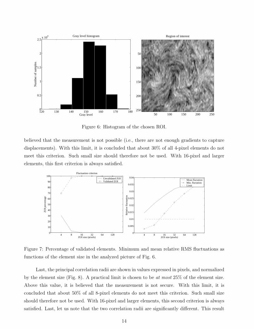
Once the picture is chosen, the software is running. Seven different results are shown. Let

us discuss them as they appear on the screen. The gray level histogram is first given for the

considered ROI (Fig. 6). In the present case, only a very small part (i.e., ca. 40 gray levels) of

the dynamic range of the CCD camera (i.e., 256 gray levels) is used. If possible, this should be

avoided and the situation shown in Fig. 2 is more desirable. If the test has not yet started, it

is time to reconsider the parameters of the camera. Otherwise, it is too late, and one will have

to do with what one has.

The fluctuation properties are given next (Fig. 7). The normalized RMS value with respect

to the dynamic range of the picture is plotted as a function of the element size. A practical

limit is chosen to be at least 1% of the dynamic range of the camera. Below this value, it is

13

120 130 140 150 160 170 1800

0.5

1

1.5

2

2.5x 10

4 Gray level histogram

Gray level

Num

ber

of s

ampl

esRegion of interest

50 100 150 200 250

50

100

150

200

250

Figure 6: Histogram of the chosen ROI.

believed that the measurement is not possible (i.e., there are not enough gradients to capture

displacements). With this limit, it is concluded that about 30% of all 4-pixel elements do not

meet this criterion. Such small size should therefore not be used. With 16-pixel and larger

elements, this first criterion is always satisfied.

4 8 16 32 64 1280

10

20

30

40

50

60

70

80

90

100Fluctuation criterion

ZOI size (pixels)

ZO

I pe

rcen

tage

Unvalidated ZOIValidated ZOI

4 8 16 32 64 1280

0.005

0.01

0.015

0.02

0.025

0.03

0.035

0.04

ZOI size (pixels)

Rel

ativ

e fl

uctu

atio

n

Mean fluctationMin. fluctationLimit

Figure 7: Percentage of validated elements. Minimum and mean relative RMS fluctuations as

functions of the element size in the analyzed picture of Fig. 6.

Last, the principal correlation radii are shown in values expressed in pixels, and normalized

by the element size (Fig. 8). A practical limit is chosen to be at most 25% of the element size.

Above this value, it is believed that the measurement is not secure. With this limit, it is

concluded that about 50% of all 8-pixel elements do not meet this criterion. Such small size

should therefore not be used. With 16-pixel and larger elements, this second criterion is always

satisfied. Last, let us note that the two correlation radii are significantly different. This result

14

indicates that the texture is anisotropic (Fig. 6). The interested reader will find additional

details in Ref. [18] concerning the determination of dominant orientations of a texture.

4 8 16 32 64 1280

10

20

30

40

50

60

70

80

90

100Correlation radius criterion

ZOI size (pixels)

ZO

I pe

rcen

tage

Unvalidated ZOIValidated ZOI

4 8 16 32 64 1280

0.5

1

1.5

2

2.5

3

3.5

4

4.5

5

ZOI size (pixels)

Dim

ensi

onle

ss c

orre

latio

n ra

dii

R1meanR1max R2meanR2max Limit

4 8 16 32 64 1280

2

4

6

8

10

12

14

16

18

20

ZOI size (pixels)

Cor

rela

tion

radi

i (pi

xels

)

R1meanR1max R2meanR2max

Figure 8: Percentage of validated elements. Maximum and mean correlation radii as functions

of the element size.

With these two simple criteria, it is concluded that at least 16-pixel elements are to

be chosen (i.e., both are satisfied simultaneously). It is worth noting that this first a priori

analysis concerns only the texture itself. It is therefore a qualitative analysis. In the following,

two quantitative analyses are proposed.

3.1.2 Displacement uncertainty

Prior to any computation, it is important to estimate the a priori performance of the approach

on the actual texture of the image. If one changes the picture, one may not get exactly the

same performance since it is related to the local details of the gray level distribution as shown

in Section 2. This is performed by using the original image f only, and generating a translated

image g by a prescribed amount upre. Such an image is generated in Fourier space using a simple

phase shift for each amplitude. This procedure implies a specific interpolation procedure for

inter-pixel gray levels, to which one resorts systematically (see Section 2.3). The algorithm is

then run on the pair of images (f, g), and the estimated displacement field uest(x) is measured.

One is mainly interested in sub-pixel displacements, where the main origin of errors comes

from inter-pixel interpolation. Therefore the prescribed displacement is chosen along the (1, 1)

direction so as to maximize this interpolation sensitivity. To highlight this reference to the

pixel scale, one refers to the x- (or y-) component of the displacement upre ≡ upre.ex varying

from 0 to 1 pixel, rather than the Euclidian norm (varying from 0 to√

2 pixel).

The quality of the estimate is characterized by two indicators, namely, the systematic

error, δu = ‖〈uest〉 − upre‖, and the standard uncertainty σu = 〈‖uest − 〈uest〉‖2〉1/2. The

change of these two indicators is shown in Fig. 9 as functions of the prescribed displacement

amplitude for different element sizes ` ranging from 4 to 128 pixels. Both quantities reach a

15

maximum for one half pixel displacement, upre = 0.5 pixel, and are approximately symmetric

about this maximum. Integer valued displacements (in pixels) imply no interpolation and are

exactly captured through the multi-scale procedure discussed above. This confirms that these

errors are due to interpolation procedures. The results are shown in a semi-log scale to reveal

the strong sensitivity to the element size, however a linear scale would show that both δu and σu

follow approximately a linear increase with upre from 0 to 0.5 pixel (and a symmetric decrease

from 0.5 to 1 pixel).

10-6

10-5

10-4

10-3

10-2

10-1

0 0.2 0.4 0.6 0.8 1

4

8

16

32

64

128

Prescribed displacement (pixel)

-a-

Mea

n d

ispla

cem

ent

erro

r (p

ixel

)

10-5

10-4

10-3

10-2

10-1

100

0 0.2 0.4 0.6 0.8 1

4

8

16

32

64

128

Sta

nd

ard u

nce

rtai

nty

(pix

el)


-b-

Figure 9: Mean error δu and standard deviation σu as a function of the prescribed displacement

upre for different element sizes ` ranging from 4 to 128 pixels.

To quantify the effect of the element size, the error and standard uncertainty, are averaged

over upre within the range [0, 1] as functions of the element size `. These data are shown in

Fig. 10. A power-law decrease

〈σu〉 = A1+ζ`−ζ

〈δu〉 = B1+υ`−υ(14)

for 8 ≤ ` ≤ 128 pixels is usually observed as shown by a regression line on the graph. Both

amplitudes are typically close to 1 pixel (more precisely A = 1.15 pixel and B = 1.07 pixel).

The exponents are measured to be ζ = 1.96 and υ = 2.34. The data for ` = 128 pixels seem

to depart from the power-law trend with a tendency to saturate. These results quantify the

trade-off the experimentalist has to face in the analysis of a displacement field, namely, either

the measurement is accurate but estimated over a large zone, or it is spatially resolved but at

the cost of a less accurate determination. This is a significant difference with classical finite

element techniques for which convergence is achieved when the element size decreases. This

is not the case when measurements are concerned. Let us however underline the following

conclusions:

16

• Elements as small as ` = 4 pixels may be used with an average error and standard

uncertainty of the order of 0.1 pixel,

• Systematic errors of the order of 10−2 and 10−3 pixel is reached for element sizes respec-

tively equal to 8 and 16 pixels.

• Standard uncertainties of the order of 2× 10−2 and 6× 10−3 pixel is reached for element

sizes respectively equal to 8 and 16 pixels.

• The systematic error in the determination of a displacement is such that evaluations will

be “attracted” toward integer values. Correspondingly, transitions at half-integer pixel

values for the displacement will appear as more abrupt. This phenomenon will be referred

to as “integer locking” in the sequel, and will be discussed in detail. Let us underline

that this spurious bias is revealed in this technique because the latter is used down to

extremely small element sizes.

"!$# % &')( *+% ,- .

/ 0'/

1'1"2-3 465 789 3 465 7

: ; <

"!$# % &'=( *+% ,- .

/ >$/

Figure 10: Average error 〈δu〉 and standard uncertainty 〈σu〉 as functions of the element size

`. For the displacement uncertainty, the results obtained by Q4-DIC are compared with those

obtained by FFT-DIC. The dashed lines correspond to power-law fits.

For comparison purposes, the displacement uncertainties obtained with the present tech-

nique are compared with those of a standard FFT-DIC technique [10]. In that case, a weaker

power-law decrease is observed with A = 1.00 pixel and ζ = 1.23 (Fig. 10b). This result shows

that by using a continuous description of the displacement field, it enables for a decrease of the

displacement uncertainty when the same element size is used. Conversely, for a given displace-

ment uncertainty, the Q4-DIC algorithm allows one to reduce significantly the element size,

17

thereby increasing the number of measurement points when compared to a classical FFT-DIC

technique.


The same instructions as presented for the texture analysis (Section 3.1.1) hold. We reproduce

them for a more linear reading. Choose the Uncertainty option in the first menu. Another

menu appears in which the format of the pictures is chosen (Fig. 4):


.png, .tif.


B/W .bmp files.



B/W .jpg files.


B/W .png files.








the ROI (Fig. 5).


(Fig. 5).




18






image.

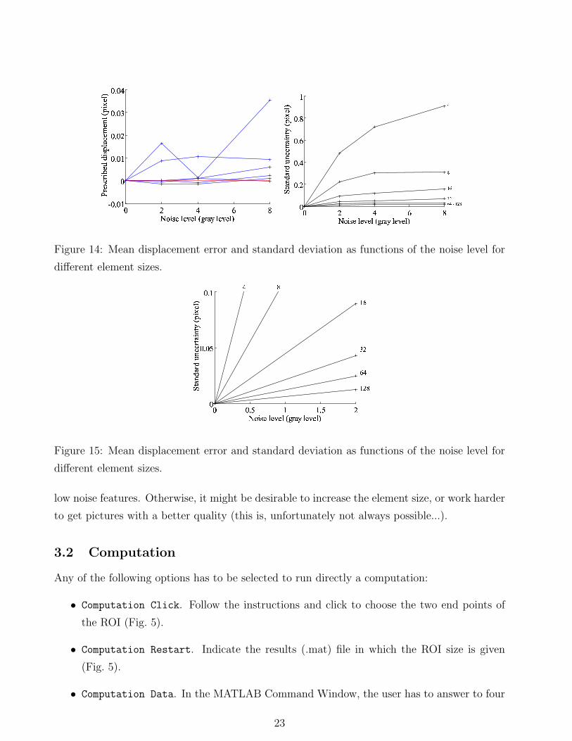
Once the picture is chosen, the software is running. It consists in artificially moving a

picture with a constant rigid body motion. In practice, increments of 0.5 pixel are sufficient

since the mean error and corresponding standard deviation are piece-wise linear functions of the

prescribed displacement (Fig. 9). Four different results are shown. The mean displacement error

and corresponding standard deviation are plotted as functions of the prescribed displacement

for different element sizes (Fig. 11). In the present case, there is a significant decrease as the

element size becomes greater than or equal to 16 pixels.

0 0.2 0.4 0.6 0.8 10

0.05

0.1

0.15

0.2

0.25

0.3

0.35


Stan

dard

unc

erta

inty

(pi

xel)

4 8 163264

0 0.2 0.4 0.6 0.8 10

0.005

0.01

0.015

0.02

0.025

0.03

0.035


Mea

n er

ror

(pix

el)

4 8 163264

Figure 11: Mean displacement error and standard deviation as functions of the prescribed

displacement for different element sizes.

The average displacement error and standard deviation are also given and power law

fitted. Figure 12 shows first that the mean error is an order of magnitude less than the standard

deviation. This result shows that the measurements are basically unbiased but mildly scattered

around the true value. Second, the standard deviation decreases as the element size increases

as already discussed above (namely, either the measurement is accurate but generally estimated

over a large zone, or it is spatially resolved but at the cost of a less accurate determination).

With this second analysis, it is concluded that 16-pixel elements can be chosen and that

the displacement uncertainty is of the order of 2× 10−2 pixel. When compared with the results

of Fig. 10, it is concluded that the artificial texture (Fig. 2) yields lower levels of displacement

uncertainties than the stone wool texture.

19

"! #$ %'&)( *+-, ! .0/132405'6 798:<;>=

?@BACDFEGBHIJDFKLGNMOCP

QR STU VWXYXZ[ X\\]\^ TR _XU`

! #"#$!%'&)( *+-, .0/1325476

89;:<>=@?A;BCD=@EFAHG#<>I

JK LMN OPQRQST USPQVT OK ST WX MK YQNZ

[]\^ _`_

Figure 12: Mean displacement error and standard deviation as functions of the element size.

3.1.3 Noise sensitivity

Last, the effect of noise associated to the image acquisition (e.g., digitization, read-out noise,

black current noise, photon noise [20]) on the displacement measurement is assessed. This anal-

ysis allows one to estimate the displacement resolution [21]. The reference image is corrupted

by a Gaussian noise of zero mean and standard variation σg ranging from 1 to 8 gray levels

at each pixel with no spatial correlation. No displacement field is superimposed on the image,

and the displacement field is then estimated. The standard deviation of the displacement field,

σu, is shown in Fig. 13 as a function of the noise amplitude σg and for different element sizes

ranging from 4 to 128 pixels. The quantity σu is linear in the noise amplitude and inversely pro-

portional to the element size. The latter properties are derived from the central limit theorem.

A theoretical analysis of this problem is discussed in Refs. [11, 22], and leads to the

following estimate of the standard deviation of the displacement field induced by a Gaussian

white noise

σu =12√

2σgp

7〈|∇f |2〉1/2`(15)

where p is the physical pixel size. For the present application, one computes 〈|∇f |2〉1/2 ≈5340 pixel−1, hence σu ≈ 4.5× 10−4σgp/`. This theoretical expectation (neglecting the spatial

correlation in the image texture) is consistent with the direct estimates shown in Fig. 13 (e.g.,

for ` = 4 pixels and σg = 8 gray levels, the direct estimate is 1.2×10−3 pixel to be compared with

9× 10−4 pixel given by the above formula). In practice, with the used CCD camera, the noise

level is given with a maximum range less than 3 gray levels. Consequently, the contribution of

20

0 2 4 6 80

0.5

1

1.5x 10

Noise level (gray level)

Stan

dard

unc

erta

inty

(pix

el)

4

8

16

3264128

-3

Figure 13: Standard deviation of the displacement error versus noise amplitude for different

element sizes (4, 8, 16, 32, 64 and 128 pixels) from top to bottom.

image noise is negligibly small when compared to that induced by the sub-pixel interpolation.


The same instructions as presented for the texture analysis (Section 3.1.1) hold. We reproduce

them for a more linear reading. Choose the Resolution option in the first menu. Another

menu appears in which the format of the pictures has to be chosen (Fig. 4):


.png, .tif.


B/W .bmp files.



B/W .jpg files.


B/W .png files.




21





the ROI (Fig. 5).


(Fig. 5).









image.

Once the picture is chosen, the software is running. It consists in adding varying levels of

random Gaussian noise to the reference picture and then performing the correlation calculation

with respect to the reference picture. Two different results are shown. The mean displacement

error and corresponding standard deviation are plotted as functions of the noise level (standard

deviation) for different element sizes (Fig. 14). The mean error has usually a very erratic trend

(this is only a check) and very low values. Conversely, the standard deviation has a clearer

tendency already discussed above.

In the present case however, the results have to be analyzed very carefully. The levels

are very high. This is to be related to the low dynamic range of the analyzed picture (Fig. 6)

that makes the texture very sensitive to acquisition noise. Figure 15 shows a zoom around

the 0-2 gray level standard deviation range. It is concluded that in the present case, the main

limitation in terms of performance is induced by the texture itself, and not the correlation

algorithm. This is an extreme case. In many situations, the result is just the opposite (namely,

the correlation code bears most of the “responsibility,” in particular when artificial textures

are considered as shown above).

With this third analysis, it is concluded that 16-pixel elements can be chosen and that

the displacement uncertainty is of the order of 2× 10−2 pixel, provided the camera sensor has

22

! #"%$&('

) *+,-*./ +00. ,12 3-+4+567 1. 8+29

!#"

$ % &'( &)( *'+,)% &- '% ./ 0- 1,23 4

56 78:97 4; 6 95

Figure 14: Mean displacement error and standard deviation as functions of the noise level for

different element sizes.

!#"

$ % &'( &)( *'+,)% &- '% ./ 0- 1,23

4 5687

9 :

7 46:;5

Figure 15: Mean displacement error and standard deviation as functions of the noise level for

different element sizes.

low noise features. Otherwise, it might be desirable to increase the element size, or work harder

to get pictures with a better quality (this is, unfortunately not always possible...).

3.2 Computation

Any of the following options has to be selected to run directly a computation:


the ROI (Fig. 5).


(Fig. 5).


23








image.

Another menu appears in which the format of the pictures has to be selected (Fig. 4):


.png, .tif.


B/W .bmp files.



B/W .jpg files.


B/W .png files.




The reference image, which is not necessarily located in the same directory as CORRELIQ4, has

to be selected (Fig. 4). In the next menu (Fig. 16), the parameters of the correlation method

have to be chosen:

• The size of the elements (typically 16 × 16 pixels). This is one of the most critical one.

The a priori analysis should therefore help in choosing it. In the present version, only

even numbers can be selected.

• The shift δ between to neighboring zones. This option is not active with a Q4 algorithm.

24

• The number of scales is the second most important parameter. As discussed above, the

present algorithm is based upon a coarse-graining approach. When large displacements

and / or strains are suspected to occur, it is desirable to increase the number of scales.

The maximum number of scales depends on the size of the ROI in comparison to that

of the elements (e.g., for a 512 × 512pixel-ROI, and 16-pixels elements, the maximum

number of scales is 5, i.e., at least 2× 2 elements are needed for the coarsest scale).

• The number of iterations (the higher the number, the higher the accuracy and the com-

putation time). This value is given to avoid endless iterations. This criterion should not

be reached. In case it is reached a message warns the user:

--------------------------- WARNING - WARNING -----------------------------

Warning: No convergence: check results!!

--------------------------- WARNING - WARNING -----------------------------

• The number of images to analyze (the reference image is not included in that count);

• When a sequence of more than one image is considered, the correlation can be performed

either by considering always the same reference image for strains (in absolute value) less

than or equal to 10% or by changing (or updating) the reference image. In the last case,

the Image update Y/N has to be activated.

• Last, it is possible to store the correlation results for any couple of analyzed pictures.

This is made possible by activating the Independent calculation Y/N button.

Validate the choice at the end (press the Validation button).

The sequence of deformed pictures has to be selected. The user selects the whole sequence

by using the same procedure as for the reference picture (Fig. 17).

It is then possible to mask part of the ROI. A menu appears and seven different operations

are possible:

• Define exclusion polygon allows the user by mouse click to enter different exclusion

regions. Follow the instructions on top of the picture that appears.

• Remove polygon allows the user by mouse click to remove any of the existing exclusion

polygon.

25

• Define exclusion circle allows the user, for instance to mask a hole. Follow the

instructions on top of the picture that appears.

• Remove exclusion circle allows the user by mouse click to remove any of the existing

exclusion circle.

• Define inclusion circle allows the user to choose a circular ROI from a rectangular

shape chosen before. This would be the case for the analysis of a Brazilian test [12].

Follow the instructions on top of the picture that appears.

• Remove inclusion circle allows the user by mouse click to remove any of the existing

inclusion circle.

• Redraw when the user is not happy with the (random) colors.

• Exit to end the mask procedure.

When the computation is completed, the result file has to be saved (Fig. 18). The extension

is ‘.mat’ to be readable for a later visualization. The computation is now ended and the

visualization stage starts. One can choose to perform another computation or to visualize any

Figure 16: dialog box for choosing the correlation parameters.

26

Figure 17: dialog box to choose the deformed picture(s).

Figure 18: dialog box to choose the type of mask and to save the results

results. Type the command correli_q4 at the MATLAB prompt. It can be noted that during

the computations, different messages may appear. Some messages are only given to indicate

that the computation is running normally.

3.3 Visualization

If Visualization is chosen, the result file (‘.mat’ extension) to be displayed has to be selected

(Fig. 19).

Figure 20 appears, in which different options can be chosen. In the present case, the

vertical displacement field (expressed in pixels) is plotted for the stone wool texture for which

an artificially deformed picture was created. A uniform nominal strain level of 0.25 was applied.

This is an extreme case for the present correlation software that needs all the scales to capture

properly the displacement field. The element size was equal to 16 pixels. It is worth noting

that the maximum displacements are greater than 3 times the element size. Had the multiscale

algorithm not been implemented, it would have been impossible to capture these levels (i.e., 5

27

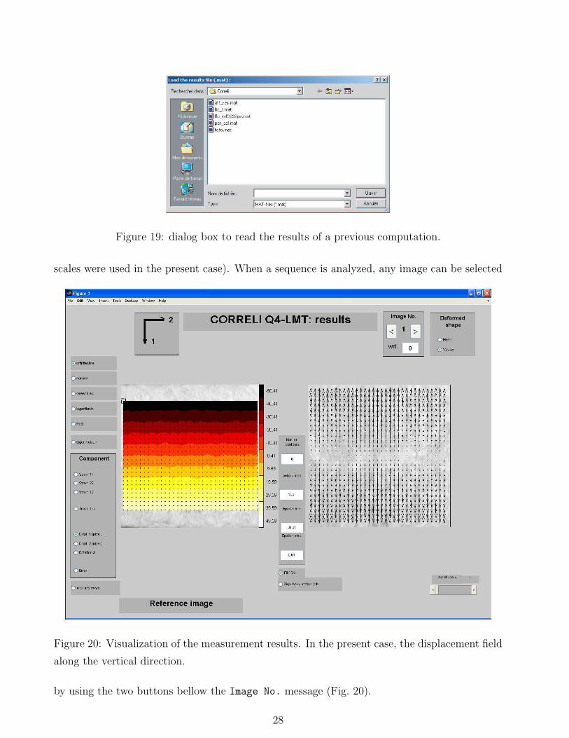
Figure 19: dialog box to read the results of a previous computation.

scales were used in the present case). When a sequence is analyzed, any image can be selected

Figure 20: Visualization of the measurement results. In the present case, the displacement field

along the vertical direction.

by using the two buttons bellow the Image No. message (Fig. 20).

28

At the top left corner are options related to the strain measures:

• infinitesimal: infinitesimal strains (i.e., symmetric part of displacement gradient, see

Eq. (24));

• nominal: nominal (Cauchy-Biot) strains (Eq. (58), when m = 1/2);

• Green Lag.: Green-Lagrange strains (Eq. (58), when m = 1);

• logarithmic: logarithmic (Hencky) strains (Eq. (58), when m → 0+);

• RdB (internal development);

• Eigen value?: the eigen values of the selected strain measure are shown.

It is worth noting that in the case of large strains (see details in the Appendix), the out-of-

plane displacement is assumed to be small and is therefore neglected. Other assumptions can

be made. They will have to be implemented on demand.

Just below are options related to the type of component to visualize. The type of com-

ponent to display has to be chosen, namely, in-plane strains, in-plane displacements, or out-of-

plane rotation. The frame is always the same, namely, horizontal direction: 2, vertical direction:

1. By choosing error, an error indicator (i.e., correlation residual |u(x).∇f(x)+ f(x)− g(x)|normalized by the dynamic range of the picture) of the result is plotted. The closer to 0, the

better the result (when no lighting variations occur, levels below few percentages are usually

achieved).

Two pictures are plotted. The left picture is always the very first reference picture. For

the reference image, the chosen field is plotted. In the case of displacements, the average value

is always in the middle of the scale. To change the scale, the dialog box in between the two

images is to be used (Fig. 21).

The number of contours can be changed. If 0 is set, a grayscale is used. If 11 is chosen,

a fancy color scale appears, otherwise a conventional (i.e., hot) one is used. The amplitude of

the displacement field is chosen with respect to the average value. For strains, two routes can

be followed:

• the maximum and minimum values are given by the user in the middle part of the dialog

box;

• the w or w/o mean button is activated and the average value corresponds to the middle

of the scale, the range of which is chosen as the maximum strain.

29

Figure 21: Contour and scale options. Mesh options. Amplification of the displacements.

When the fill option is activated, the contours are filled on the reference image. The rigid

body motion can be subtracted to the overall displacement by pushing the corresponding button

(Rigid body motion Y/N). When the error indicator is plotted, there is no need to change any

scale parameters, it is performed automatically. The w or w/o mean button can also be used.

When selecting mesh, the undeformed and deformed meshes appear on the relevant images

(Fig. 22). When selecting vector, the displacement vectors are shown (Fig. 21). It can be noted

that both options can be used simultaneously. A slider enables the displacements to be amplified

by a factor that can be chosen by the user (Fig. 21). When the amplification is greater than 1,

the underlying image disappears.

To further comment on the results on the artificially deformed picture, the corresponding

(nominal) strain field is shown in Fig. 22. Since the w or w/o mean button is activated, the

average strain can be read directly as the median value (i.e., 0.2396 ≈ 0.24 for a prescribed

value of 0.25).

3.4 Virtual Gauges

Type the command gauge at the MATLAB prompt. This procedure allows for the computation

of the average strain in a user-selected ROI. one needs to indicate the result file in which all

the data needed are stored. Then the Region Of Interest (ROI) is selected by mouse. Click and

maintain to select the ROI. If the ROI is larger than the mesh, then the size is automatically

reset to the maximum size.

In the MATLAB Command Window, average values of different strain tensors are given.

30

Figure 22: Visualization of post-processed results. In the present case the normal (nominal)

strains along the vertical direction.

The corresponding eigen strains are also computed. The results can also be saved in an ASCII

file. The computation is now ended. Type any command at the MATLAB prompt.

4 Application to a tensile test

In this section, an application of the previously proposed algorithm is carried out to analyze

a tensile test performed on an aluminum alloy sample. In the plastic regime, the formation

of localization strain bands is observed. The fact that for a given displacement uncertainty,

smaller element sizes can be chosen in the present case (Q4-DIC) when compared with those

of a standard FFT-DIC technique (Fig. 10b), enables one to better capture kinematic details

in the localization band.

31

4.1 Material and method

The studied aluminum alloy is of type 5005 (i.e., more than 99 wt% of Al content and a small

amount of Mg; these values were determined by electron probe micro-analysis). As shown in

Fig. 2, the sample is a coated with sprayed black and white paints to create the random texture

for the displacement field measurement. The sample size is 140× 30× 2 mm3. It is positioned

within hydraulic grips of a 100 kN servo-hydraulic testing machine. Its alignment is checked

with DIC measurements (i.e., no significant rotation of the sample is observed in the elastic

domain). To have a first strain evaluation, an extensometer was used. Its pins are observed on

the right edge of the sample (Fig. 2).

An artificial light source is used to minimize gray level variations so that the conservation

of the optical flow is considered as practically achieved. A CCD camera (12-bit digitization,

noise less than 3 gray levels, resolution: 1024 × 1280 pixels) with a conventional zoom is

positioned in front of the sample. In the present case, the physical size of one pixel is 25 µm.

Two loading sequences are carried out. First, in the elastic domain, a controlled displacement

rate of 5 µm/s is applied and pictures are taken for 12 µm-increments. Elastic properties may

be identified [23]. This will not be discussed herein. Second, a controlled displacement rate of

10 µm/s is applied to study strain localization and pictures are taken for 60 µm-increments.

The following analysis of the displacement field is an increment between two image acquisitions

in the “plastic” regime.

Figure 23 shows the change of the average longitudinal strain with the number of pictures

(or equivalently with time). This result was obtained by using the Q4-DIC analysis. Until the

extensometer pins slipped (at about a 5% strain), the average strain measured by DIC and

that given by the extensometer were close, even though the same surface was not analyzed.

This response is typical of a Portevin-Le Chatelier (PLC) phenomenon or jerky flow [24].

From a microscopic point of view, PLC effects are related to dynamic interactions between

mobile dislocations and diffusing solute atoms [25, 26]. From a macroscopic perspective, it is

related to a negative strain rate sensitivity that leads to localized bands that are simulated [27].

Many experimental studies [28] however are based upon average strain measurements. There

are also full-field displacement measurements performed by using, for instance, laser speckle

interferometry [29]. Yet the spatial resolution did not allow for an analysis of the displacement

field within the band. Additional insight is gained by using IR thermography [30].

32

! "$#%'&)(#*,+&-%

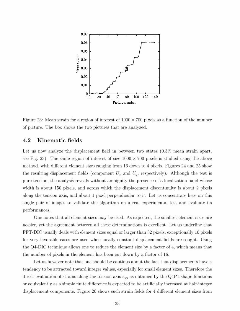
Figure 23: Mean strain for a region of interest of 1000× 700 pixels as a function of the number

of picture. The box shows the two pictures that are analyzed.

4.2 Kinematic fields

Let us now analyze the displacement field in between two states (0.3% mean strain apart,

see Fig. 23). The same region of interest of size 1000 × 700 pixels is studied using the above

method, with different element sizes ranging from 16 down to 4 pixels. Figures 24 and 25 show

the resulting displacement fields (component Ux and Uy, respectively). Although the test is

pure tension, the analysis reveals without ambiguity the presence of a localization band whose

width is about 150 pixels, and across which the displacement discontinuity is about 2 pixels

along the tension axis, and about 1 pixel perpendicular to it. Let us concentrate here on this

single pair of images to validate the algorithm on a real experimental test and evaluate its

performances.

One notes that all element sizes may be used. As expected, the smallest element sizes are

noisier, yet the agreement between all these determinations is excellent. Let us underline that

FFT-DIC usually deals with element sizes equal or larger than 32 pixels, exceptionally 16 pixels

for very favorable cases are used when locally constant displacement fields are sought. Using

the Q4-DIC technique allows one to reduce the element size by a factor of 4, which means that

the number of pixels in the element has been cut down by a factor of 16.

Let us however note that one should be cautious about the fact that displacements have a

tendency to be attracted toward integer values, especially for small element sizes. Therefore the

direct evaluation of strains along the tension axis εyy as obtained by the Q4P1-shape functions

or equivalently as a simple finite difference is expected to be artificially increased at half-integer

displacement components. Figure 26 shows such strain fields for 4 different element sizes from

33

200 400 600

-a-

800 1000

100

200

300

400

500

600

700

800200 400 600

-b-

800 1000

100

200

300

400

500

600

700

800

200 400 600

-c-

800 1000

100

200

300

400

500

600

700

800

0.6

0.4

0.2

0

0.2

0.4

200 400 600

-d-

800 1000

100

200

300

400

500

600

700

800

200 400 600

-e-

800 1000

100

200

300

400

500

600

700

800200 400 600

-f-

800 1000

100

200

300

400

500

600

700

800

Figure 24: Map of Uy displacement for different element sizes: (a) ` = 16, (b) ` = 12, (c)

` = 10, (d) ` = 8, (e) ` = 6 and (f) ` = 4 pixels. The physical size of one pixel is equal to

25 µm.

16 down to 8 pixels. For a size of 16 pixels, the localization band appears as a genuine zone

of increased strains as compared to a “silent” (or elastic) background. For smaller element

sizes, the edges of the shear band appear to concentrate still a higher strain. The same effect

is apparent for element sizes 12, 10 and 8 pixels. The strain maps obtained for smaller element

sizes are not shown, since the noise level becomes much higher and thus the measurement

cannot be trusted. The same artefact of strain enhancement at the edges of the shear band is

however observed.

34

200 400 600

-a-

800 1000

100

200

300

400

500

600

700

800

200 400 600

-b-

800 1000

100

200

300

400

500

600

700

800

200 400 600

-c-

800 1000

100

200

300

400

500

600

700

800

0

0.5

1

1.5

2

200 400 600

-d-

800 1000

100

200

300

400

500

600

700

800

200 400 600

-e-

800 1000

100

200

300

400

500

600

700

800

200 400 600

-f-

800 1000

100

200

300

400

500

600

700

800

Figure 25: Map of Ux displacement for different element sizes: (a) ` = 16, (b) ` = 12, (c)

` = 10, (d) ` = 8, (e) ` = 6 and (f) ` = 4 pixels. The physical size of one pixel is equal to

25 µm.

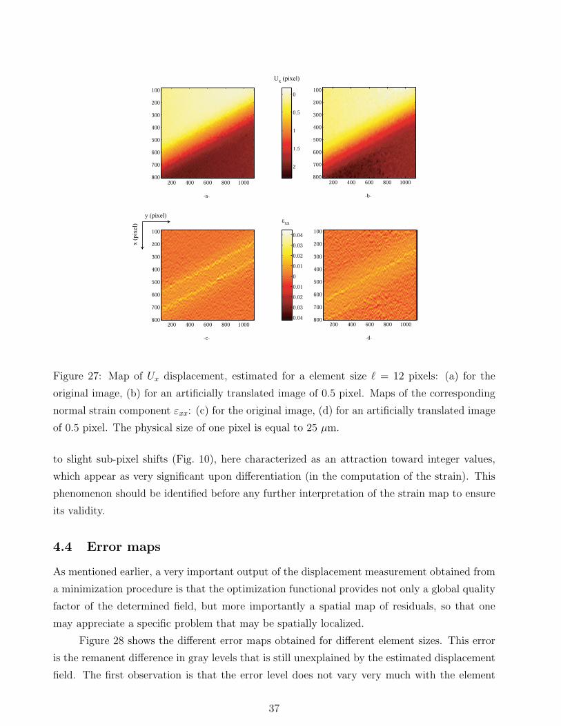
4.3 Integer locking

One notes on the previous figure that the Uy-displacement is half-integer valued at the edge of

the shear band. The larger strains at the edge of the band could therefore be interpreted as an

artefact due to integer locking. Integer valued displacements being favored, an artificial gap is

created for half-integer values displacement, and thus any gradient (finite difference operator)

will underline this effect very markedly.

To test this interpretation, the following test is proposed. An artificially translated image

by 0.5 pixel is computed from the original one, using a fast Fourier transform, as the latter

35

200 400 600

-a-

800 1000

100

200

300

400

500

600

700

800200 400 600

-b-

800 1000

100

200

300

400

500

600

700

800

200 400 600

-c-

800 1000

100

200

300

400

500

600

700

800

0.015

0.01

0.005

0

0.005

0.01

0.015

0.02

0.025

εxx

y (pixel)

x (

pix

el)

200 400 600

-d-

800 1000

100

200

300

400

500

600

700

800

Figure 26: Map of the strain component εxx for different element sizes: (a) ` = 16, (b) ` = 12,

(c) ` = 10 and (d) ` = 8 pixels.

provides a simple and numerically efficient way of interpolating the image at any arbitrary sub-

pixel value. A genuine strain enhancement is thus expected to be identified at a fixed position

in the reference image frame of coordinates, whereas a numerical artefact would be moved to

a different location. Figures 27a and b show the Uy displacement component starting from

the original image or from the translated one (and where the 1/2 pixel translated has been

corrected for). A good agreement is observed for the displacement field thus revealing a rather

poor sensitivity to such a rigid translation. Figures 27c and d show the corresponding εyy strain

maps. On the latter set of figures, although high strain values tend to concentrate along two

lines in both figures, the precise location of these bands is not stable. This is a signature of the

integer locking phenomenon. Therefore the strain enhancement at the edge of the shear band

is to be considered as an artefact.

Let us underline that such a phenomenon results from the fact that the elements are

reduced to a very small size, and still provide a very accurate determination of the displacement

field, without much noise. Such a success encourages the user to decrease the size of the elements

to very small values. By doing so, the determination of the displacement is much more prone

36

200 400 600

-a-

800 1000

100

200

300

400

500

600

700

800

2

1.5

1

0.5

0

Ux (pixel)

200 400 600

-b-

800 1000

100

200

300

400

500

600

700

800

200 400 600

-c-

800 1000

100

200

300

400

500

600

700

8000.04

0.03

0.02

0.01

0

0.01

0.02

0.03

0.04

εxx

y (pixel)

x (

pix

el)

200 400 600

-d-

800 1000

100

200

300

400

500

600

700

800

Figure 27: Map of Ux displacement, estimated for a element size ` = 12 pixels: (a) for the

original image, (b) for an artificially translated image of 0.5 pixel. Maps of the corresponding

normal strain component εxx: (c) for the original image, (d) for an artificially translated image

of 0.5 pixel. The physical size of one pixel is equal to 25 µm.

to slight sub-pixel shifts (Fig. 10), here characterized as an attraction toward integer values,

which appear as very significant upon differentiation (in the computation of the strain). This

phenomenon should be identified before any further interpretation of the strain map to ensure

its validity.

4.4 Error maps

As mentioned earlier, a very important output of the displacement measurement obtained from

a minimization procedure is that the optimization functional provides not only a global quality

factor of the determined field, but more importantly a spatial map of residuals, so that one

may appreciate a specific problem that may be spatially localized.

Figure 28 shows the different error maps obtained for different element sizes. This error

is the remanent difference in gray levels that is still unexplained by the estimated displacement

field. The first observation is that the error level does not vary very much with the element

37

size. This is consistent with the fact that the displacement field is quite comparable for different

element sizes. However, there is a slight increase in the error as the element size decreases. This

is explained by the fact that the performance of the correlation algorithm degrades as the spatial

resolution improves. This observation is in good agreement with the results to be expected from

the analysis of Fig. 10.

Figure 28: Map of the residual error η for different element sizes: (a) ` = 16, (b) ` = 12, (c)

` = 10 (d) ` = 8, (e) ` = 6 and (f) ` = 4 pixels.

5 Applications of CORRELIQ4

In the following, different references are given in which the software was used. The abstract is

given for the reader to select the relevant ones. The name of the .pdf file is also given.

38

5.1 Reference paper

G. Besnard, F. Hild and S. Roux, “Finite-element” displacement fields analysis from digital

images: Application to Portevin-Le Chatelier bands, Exp. Mech. 46 (2006) 789-803. EM2.pdf

This is the paper in which the so-called Q4-DIC technique is discussed in details. A new

methodology is proposed to estimate displacement fields from pairs of images (reference and

strained) that evaluates continuous displacement fields. This approach is specialized to a finite-

element decomposition, therefore providing a natural interface with a numerical modeling of

the mechanical behavior used for identification purposes. The method is illustrated with the

analysis of Portevin-Le Chatelier bands in an aluminum alloy sample subjected to a tensile test.

A significant progress with respect to classical digital image correlation techniques is observed

in terms of spatial resolution and uncertainty.

5.2 Identification of elastic properties

F. Hild and S. Roux, Digital image correlation: from measurement to identification of elastic

properties - A review, Strain 42 (2006) 69-80. Strain1.pdf

The current state of the art of digital image correlation, where displacements can be deter-

mined for values less than one pixel, enables one to better characterize the behavior of materials

and the response of structures to external loads. A general presentation of the extraction of

displacement fields from pictures taken at different instants during an experiment is given.

Different strategies can be followed to determine sub-pixel displacements. New identification

procedures are then devised making use of full-field measurements. A priori or a posteriori

routes can be followed. They are illustrated on the analysis of a Brazilian disk test.

5.3 SIF measurements

S. Roux and F. Hild, Stress intensity factor measurements from digital image correlation: post-

processing and integrated approaches, Int. J. Fract. 140 [1-4] (2006) 141-157. IJF4.pdf

Digital image correlation is an appealing technique for studying crack propagation in

brittle materials such as ceramics. A case study is discussed where the crack geometry, and

the crack opening displacement are evaluated from image correlation by following two different

measurement and identification routes. The displacement uncertainty can reach the nanometer

range even though optical pictures are dealt with. The stress intensity factor is estimated with

a 7% uncertainty in a complex loading set-up without having to resort to a numerical modeling

of the experiment.

39

R. Hamam, F. Hild and S. Roux, Stress intensity factor gauging by digital image correlation:

Application in cyclic fatigue, Strain 43 (2007) 181-192. Strain2.pdf

A fatigue crack in steel (CCT geometry) is studied via digital image correlation. The

measurement of the stress intensity factor change during one cycle is performed using a de-

composition of the displacement field onto a tailored set of elastic fields. The same analysis

is performed using two different routes, namely, the first one consists in computing the dis-

placement field using a general correlation technique providing the displacement field projected

onto finite element shape functions, and then analyzing this displacement field in terms of the

selected mechanically relevant fields. The second strategy, called integrated approach, directly

estimates the amplitude of these elastic fields from the correlation of successive images. Both

procedures give consistent results, and offer very good performances in the evaluation of the

crack tip position (uncertainty of about 20 µm for a 14.5-mm crack), and stress intensity factors

(uncertainty less than 1 MPa√

m).

J. Rethore, S. Roux and F. Hild, Noise-robust Stress Intensity Factor Determination from Kine-

matic Field Measurements, Eng. Fract. Mech. (2008) DOI: 10.1016/j.engfracmech.2007.04.018.

EFM1.pdf

Stress Intensity Factors are often estimated numerically from a given displacement field

through an interaction integral formalism. The latter method makes use of a weight, the virtual

crack extension field, which is under-constrained by first principles. Requiring a least noise

sensitivity allows one to compute the optimal virtual crack extension. Mode I and mode II

specialized fields are obtained and particularized for a given displacement functional basis. The

method is applied to an experimental case study of a crack in a silicon carbide sample, whose

displacement field is obtained by a digital image correlation technique. The optimization leads

to a very significant uncertainty reduction up to a factor 100 of the non-optimized formulation.

The proposed scheme reveals additional performances with respect to the integral domain choice

and assumed crack tip geometry, which are shown to have a reduced influence.

5.4 Analysis of elasto-plastic laws

V. Tarigopula, O. S. Hopperstad, M. Langseth, A. H. Clausen, F. Hild, O.-G. Lademo and

M. Eriksson, A Study of Large Plastic Deformations in Dual Phase Steel Using Digital Image

Correlation and FE Analysis, Exp. Mech. 48 [2] (2008) 181-196. EXME3.pdf

Large plastic deformation in sheets made of dual phase steel DP800 is studied experimen-

tally and numerically. Shear testing is applied to obtain large plastic strains in sheet metals

without strain localisation. In the experiments, full-field displacement measurements are car-

40

ried out by means of digital image correlation, and based on these measurements the strain field

of the deformed specimen is calculated. In the numerical analyses, an elastoplastic constitu-

tive model with isotropic hardening and the Cockcroft-Latham fracture criterion is adopted to

predict the observed behavior. The strain hardening parameters are obtained from a standard

uniaxial tensile test for small and moderate strains, while the shear test is used to determine

the strain hardening for large strains and to calibrate the fracture criterion. Finite Element

(FE) calculations with shell and brick elements are performed using the non-linear FE code

LS-DYNA. The local strains in the shear zone and the nominal shear stress-elongation char-

acteristics obtained by experiments and FE simulations are compared, and, in general, good

agreement is obtained. It is demonstrated how the strain hardening at large strains and the

Cockcroft-Latham fracture criterion can be calibrated from the in-plane shear test with the aid

of non-linear FE analyses.

5.5 Identification of a damage law

S. Roux and F. Hild, Digital Image Mechanical Identification (DIMI), Exp. Mech. DOI:

10.1007/s11340-007-9103-3 (2008). EXME4.pdf

A continuous pathway from digital images acquired during a mechanical test to quantita-

tive identification of a constitutive law is presented herein based on displacement field analysis.

From images, displacement fields are directly estimated within a finite element framework.

From the latter, the application of the equilibrium gap method provides the means for rigidity

field evaluation. In the present case, a reconditioned formulation is proposed for a better sta-

bility. Last, postulating a specific form of a damage law, a linear system is formed that gives a

direct access to the (non-linear) damage growth law in one step. The two last procedures are

presented, validated on an artificial case, and applied to the case of a biaxial tension of a com-

posite sample driven up to failure. A quantitative estimate of the quality of the determination

is proposed, and in the last application, it is shown that no more than 7% of the displacement

field fluctuations are not accounted for by the determined damage law.

5.6 Analyses of localized phenomena

I. Elnasri, S. Pattofatto, H. Zhao, H. Tsitsiris, F. Hild and Y. Girard, Shock enhancement of

cellular structures under impact loading: Part I Experiments, J. Mech. Phys. Solids 55 (2007)

2652-2671. JMPS2.pdf

This paper aims at showing experimental proof of the existence of a shock front in cellu-

lar structures under impact loading, especially at low critical impact velocities around 50 m/s.

41

First, an original testing procedure using a large diameter Nylon Hopkinson bar is introduced.

With this large diameter soft Hopkinson bar, tests under two different configurations (pressure

bar behind/ahead of the supposed shock front) at the same impact speed are used to obtain the

force/time histories behind and ahead of the assumed shock front within the cellular material

specimen. Stress jumps (up to 60% of initial stress level) as well as shock front speed are mea-

sured for tests at 55 m/s on Alporas foams and nickel hollow sphere agglomerates, whereas no

significant shock enhancement is observed for Cymat foams and 5056 aluminium honeycombs.

The corresponding rate sensitivity of the studied cellular structures is also measured and it

is proven that it is not responsible for the sharp strength enhancement. A photomechanical

measurement of the shock front speed is also proposed to obtain a direct experimental proof.

The displacement and strain fields during the test are obtained by correlating images shot with

a high speed camera. The strain field measurements at different times show that the shock

front discontinuity propagates and allows for the measurement of the propagation velocity. All

the experimental evidences enable us to confirm the existence of a shock front enhancement

even at quite low impact velocities for a number of studied materials.

V. Tarigopula, O. S. Hopperstad, M. Langseth, A. H. Clausen and F. Hild, A study of localisa-

tion in dual phase high-strength steels under dynamic loading using digital image correlation

and FE analysis, Int. J. Solids Struct. 45 [2] (2008) 601-619. IJSS5.pdf

Tensile tests were conducted on dual-phase high-strength steel in a Split-Hopkinson Ten-

sion Bar at a strain-rate in the range of 150600/s and in a servo-hydraulic testing machine at a

strain-rate between 10−3 and 100/s. A novel specimen design was utilized for the Hopkinson bar

tests of this sheet material. Digital image correlation was used together with high-speed pho-

tography to study strain localisation in the tensile specimens at high rates of strain. By using

digital image correlation, it is possible to obtain in-plane displacement and strain fields during

non-uniform deformation of the gauge section, and accordingly the strains associated with dif-

fuse and localized necking may be determined. The full-field measurements in high strain-rate

tests reveal that strain localisation started even before the maximum load was attained in the

specimen. An elasto-viscoplastic constitutive model is used to predict the observed stressstrain

behavior and strain localisation for the dual-phase steel. Numerical simulations of dynamic

tensile tests were performed using the non-linear explicit FE code LS-DYNA. Simulations were

done with shell (plane stress) and brick elements. Good correlation between experiments and

numerical predictions was achieved, in terms of engineering stressstrain behavior, deformed ge-

ometry and strain fields. However, mesh density plays a role in the localisation of deformation

in numerical simulations, particularly for the shell element analysis.

42

6 Beyond CORRELIQ4

In the following, different references are given in which extensions of the software were used.

The abstract is given for the reader to select the relevant ones.

6.1 XQ4-DIC

J. Rethore, F. Hild and S. Roux, Shear-band capturing using a multiscale extended digital

image correlation technique, Comp. Meth. Appl. Mech. Eng. 196 [49-52] (2007) 5016-5030.

CMAME2.pdf

Finite elements have been used recently to solve the optical flow conservation principle

invoked to determine displacement fields by digital image correlation. Inspired by these re-

cent advances, and by the computational effort that has been accomplished during the past 10

years for the simulation of discontinuities by the extended finite element method (XFEM), an

extended correlation technique is introduced for capturing shear-band like discontinuities from

images of real mechanical tests. Because of the specific information at hand (i.e., gray level

images), this extended finite element approach is included in a non-linear multi-grid solver. The

performances of the proposed approach are discussed on two examples, namely the analysis of

a bolted assembly and the formation of Piobert-Luders bands.

J. Rethore, G. Besnard, G. Vivier, F. Hild and S. Roux, Experimental investigation of localized

phenomena using Digital Image Correlation, Phil. Mag. [submitted] (2008). PM1.pdf

The present paper is dedicated to the use of enriched discretization schemes in the context

of digital image correlation. The aim is to capture and evaluate strong or weak discontinuities

of a displacement field directly from digital images. An analysis of different enrichment per-

formances is provided. Two examples of strain localization illustrate the discussion, namely,

a compression test on an HMX-based material and the Portevin-Le Chatelier band shown in

Section 4.

J. Rethore, F. Hild and S. Roux, Extended digital image correlation with crack shape opti-

mization, Int. J. Num. Meth. Eng. 73 [2] (2008) 248-272. IJNME2.pdf

The methodology of eXtended finite element method is applied to the measurement of dis-

placements through digital image correlation. An algorithm, initially based on a finite element

decomposition of displacement fields, is extended to benefit from discontinuity and singular en-

richments over a suited subset of elements. This allows one to measure irregular displacements

encountered, say, in cracked solids, as demonstrated both in artificial examples and experi-

43

mental case studies. Moreover, an optimization strategy for the support of the discontinuity

enables one to adjust the crack path configuration to reduce the residual mismatch, and hence

to be tailored automatically to a wavy or irregular crack path.

6.2 Beam-DIC

F. Hild, S. Roux, R. Gras, N. Guerrero, M. E. Marante and J. Florez-Lopez, Displacement

Measurement Technique for Euler-Bernoulli Kinematics, Opt. Lasers Eng. [accepted] (2008).

OLE1.pdf

It is proposed to develop a digital image correlation procedure that is suitable for beams

whose kinematics is described by an Euler-Bernoulli hypothesis. As a direct output, the degrees

of freedom corresponding to flexural and axial loads are directly measured. The performance

of the correlation algorithm is evaluated by using a picture of a cantilever beam experiment.

One load level is analyzed with the present algorithm. The latter is validated by comparing the

displacement field with that given by a finite element based correlation algorithm. It is also

shown that a locally buckled zone is detectable with the present procedure.

6.3 Stereo-correlation

G. Besnard, F. Hild, J.-M. Lagrange, S. Roux and C. Voltz, Contact-free characterization of

materials used in detonics experiments, Proceedings Europyro 2007 . EUROPYRO_07.pdf

In detonics experiments, specimens are loaded through intense shock waves produced by

explosives, and hence the simultaneous occurrence of large strains and high strain rates makes

the analysis delicate. Attention is here focused on tantalum whose elasto-plastic properties are

quite complex, possibly involving strain localization. In order to face this challenge, the choice

has been made to use imaging techniques, both for quasi-static tests (few images per second

at most) and dynamic experiments (up to one million frames per second). Displacement fields

are analyzed through digital image correlation techniques applied to monovision for in-plane

displacements, and stereocorrelation when the three dimensional components of the surface

displacement field are sought. Quasi-static tests on a tantalum specimen give access to the

elastic properties (Young’s modulus and Poisson’s ratio), but also reveal strain localization

occurring in the plastic flow regime. Extension of this technique to stereocorrelation is underway

in order to have access to microsecond time resolution, and sub-millimeter space resolution.

44

6.4 C8-DIC

S. Roux, F. Hild, P. Viot and D. Bernard, Three dimensional image correlation from X-Ray

computed tomography of solid foam, Comp. Part A DOI: 10.1016/j.compositesa.2007.11.011

[in press] (2008). CompPartA1.pdf

A new methodology is proposed to estimate 3D displacement fields from pairs of images

obtained from X-Ray Computed Micro Tomography (XCMT). Contrary to local approaches,

a global approach is followed herein that evaluates continuous displacement fields. Although

any displacement basis may be considered, the procedure is specialized to finite element shape

functions. The method is illustrated with the analysis of a compression test on a polypropylene

solid foam (independently studied in a companion paper). A good stability of the measured

displacement field is obtained for cubic element sizes ranging from 16 voxels to 6 voxels. This

last paper is a direct extension of Q4-DIC to three-dimensional displacement measurements in

the bulk of a material.

7 Conclusion

A novel approach was developed to determine a displacement field based on the comparison

of two digital images. The sought displacement field is decomposed onto a basis of continuous

functions using Q4P1-shape functions as proposed in finite element methods. The latter corre-

sponds to one of the simplest kinematic descriptions. It therefore allows for a compatibility of

the kinematic hypotheses made during the measurement stage and the subsequent identification

/ validation stage, for instance, by using conventional finite element techniques.

The performance of the algorithm is tested on a reference image to evaluate the reliability

of the estimation, which is shown to allow for either an excellent accuracy for homogeneous

displacement fields, or for a very well resolved displacement field down to element sizes as small

as 4×4 pixels. When compared with a standard FFT-DIC technique, Q4-DIC enables for a

significant decrease of the displacement uncertainty when the same size of the elements is used.

For the natural texture studied herein, it is shown that the main limitation is related to its

poor dynamic range that makes it very sensitive to acquisition noise.

Last, the displacement field is analyzed on an aluminium alloy sample where a localization

band develops. In the present case, it corresponds to a Portevin-Le Chatelier effect. For element

sizes ranging from 16 down to 4 pixels, the displacement field is shown to be reliably determined.

As far as strains are concerned, spurious strain concentrations at the edge of the shear band

is observed for small element sizes. This is attributed to integer locking of the displacement.

Apart from this bias, the analysis has been shown to be operational and reliable, on a real

45

experimental test with strain localization. The complete space-time kinematic analysis is now

possible for the Portevin-Le Chatelier phenomenon even within the band thanks to the spatial

resolution achieved by the Q4-DIC technique presented herein. It is deferred to a another

publication in which an enriched kinematics is implemented [31].

References

[1] P. K. Rastogi, edts., Photomechanics, (Springer, Berlin (Germany), 2000), 77.

[2] M. A. Sutton, S. R. McNeill, J. D. Helm and Y. J. Chao, Advances in Two-Dimensional and

Three-Dimensional Computer Vision, in: Photomechanics , P. K. Rastogi, eds., (Springer,

Berlin (Germany), 2000), 323-372.

[3] A. Lagarde, edt., Advanced Optical Methods and Applications in Solid Mechanics,

(Kluwer, Dordrecht (the Netherlands), 2000), 82.

[4] O. C. Zienkievicz and R. L. Taylor, The Finite Element Method , (McGraw-Hill, London

(UK), 4th edition, 1989).

[5] B. K. P. Horn and B. G. Schunck, Determining optical flow, Artificial Intelligence 17

(1981) 185-20.

[6] P. J. Hubert, Robust Statistics , (Wiley, New York (USA), 1981).

[7] M. Black, Robust Incremental Optical Flow , (PhD dissertation, Yale University, 1992).

[8] J.-M. Odobez and P. Bouthemy, Robust multiresolution estimation of parametric motion

models, J. Visual Comm. Image Repres. 6 (1995) 348-365.

[9] M. A. Sutton, W. J. Wolters, W. H. Peters, W. F. Ranson and S. R. McNeill, Determination

of Displacements Using an Improved Digital Correlation Method, Im. Vis. Comp. 1 [3]

(1983) 133-139.

[10] F. Hild, B. Raka, M. Baudequin, S. Roux and F. Cantelaube, Multi-Scale Displacement

Field Measurements of Compressed Mineral Wool Samples by Digital Image Correlation,

Appl. Optics IP 41 [32] (2002) 6815-6828.

[11] S. Roux and F. Hild, Stress intensity factor measurements from digital image correlation:

post-processing and integrated approaches, Int. J. Fract. 140 [1-4] (2006) 141-157.

46

[12] F. Hild and S. Roux, Digital image correlation: from measurement to identification of

elastic properties - A review, Strain 42 (2006) 69-80.

[13] F. Hild, S. Roux, R. Gras, N. Guerrero, M. E. Marante and J. Florez-Lopez, Displace-

ment Measurement Technique for Euler-Bernoulli Kinematics, Opt. Lasers Eng. [accepted]

(2008).

[14] B. Wagne, S. Roux and F. Hild, Spectral Approach to Displacement Evaluation From

Image Analysis, Eur. Phys. J. AP 17 (2002) 247-252.

[15] S. Roux, F. Hild and Y. Berthaud, Correlation Image Velocimetry: A Spectral Approach,

Appl. Optics 41 [1] (2002) 108-115.

[16] P. J. Burt, C. Yen and X. Xu, Local correlation measures for motion analysis: a compara-

tive study, Proceedings IEEE Conf. on Pattern Recognition and Image Processing , (1982),

269-274.

[17] H. W. Schreier, J. R. Braasch and M. A. Sutton, Systematic errors in digital image corre-

lation caused by intensity interpolation, Opt. Eng. 39 [11] (2000) 2915-2921.

[18] S. Bergonnier, F. Hild and S. Roux, Local anisotropy analysis for non-smooth images,

Patt. Recogn. 40 [2] (2007) 544-556.

[19] J.-N. Perie, S. Calloch, C. Cluzel and F. Hild, Analysis of a Multiaxial Test on a C/C

Composite by Using Digital Image Correlation and a Damage Model, Exp. Mech. 42 [3]

(2002) 318-328.

[20] G. Holst, CCD Arrays, Cameras and Displays , (SPIE Engineering Press, Washington DC

(USA), 1998).

[21] ISO, International Vocabulary of Basic and General Terms in Metrology (VIM), (Interna-

tional Organization for Standardization, Geneva (Switzerland), 1993).

[22] G. Besnard, F. Hild and S. Roux, “Finite-element” displacement fields analysis from digital

images: Application to Portevin-Le Chatelier bands, Exp. Mech. 46 (2006) 789-803.

[23] G. Besnard, Correlation d’images et identification en mecanique des solides, (University

Paris 6, Intermediate MSc report 2005).

[24] A. Portevin and F. Le Chatelier, C. R. Acad. Sci. Paris 176 (1923) 507.

[25] A. H. Cottrell, A note on the Portevin-Le Chatelier effect, Phil. Mag. 44 (1953) 829-832.

47

[26] P. G. McCormick, A model of the Portevin-Le Chatelier effect in substitutional alloys,

Acta Metall. 20 (1972) 351-354.

[27] A. H. Clausen, T. Borvik, O. S. Hopperstad and A. Benallal, Flow and fracture char-

acteristics of aluminium alloy AA5083-H116 as function of strain rate, temperature and

triaxiality, Mat. Sci. Eng. A364 (2004) 260-272.

[28] D. Thevenet, M. Mliha-Touati and A. Zeghloul, Characteristics of the propagating defor-

mation bands associated with the Portevin-Le Chatelier effect in an Al-Zn-Mg-Cu alloy,

Mat. Sci. Eng. A291 (2000) 110-117.

[29] R. Shabadi, S. Kumara, H. J. Roven and E. S. Dwarakadasa, Characterisation of PLC

band parameters using laser speckle technique, Mat. Sci. Eng. A364 (2004) 140-150.

[30] H. Louche, P. Vacher and R. Arrieux, Thermal observations associated with the Portevin-

Le Chatelier effect in an Al-Mg alloy, Mat. Sci. Eng. A 404 (2005) 188-196.

[31] J. Rethore, G. Besnard, G. Vivier, F. Hild and S. Roux, Experimental investigation of

localized phenomena using Digital Image Correlation, Phil. Mag. [submitted] (2008).

[32] R. Hill, Aspects of Invariance in Solid Mechanics, Adv. Appl. Mech. 18 (1978) 1-75.

48

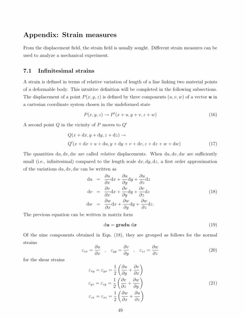
Appendix: Strain measures

From the displacement field, the strain field is usually sought. Different strain measures can be

used to analyze a mechanical experiment.

7.1 Infinitesimal strains

A strain is defined in terms of relative variation of length of a line linking two material points

of a deformable body. This intuitive definition will be completed in the following subsections.

The displacement of a point P (x, y, z) is defined by three components (u, v, w) of a vector u in

a cartesian coordinate system chosen in the undeformed state

P (x, y, z) → P ′(x + u, y + v, z + w) (16)

A second point Q in the vicinity of P moves to Q′

Q(x + dx, y + dy, z + dz) →Q′(x + dx + u + du, y + dy + v + dv, z + dz + w + dw) (17)

The quantities du, dv, dw are called relative displacements. When du, dv, dw are sufficiently

small (i.e., infinitesimal) compared to the length scale dx, dy, dz, a first order approximation

of the variations du, dv, dw can be written as

du =∂u

∂xdx +

∂u

∂ydy +

∂u

∂zdz

dv =∂v

∂xdx +

∂v

∂ydy +

∂v

∂zdz (18)

dw =∂w

∂xdx +

∂w

∂ydy +

∂w

∂zdz.

The previous equation can be written in matrix form

du = gradu dx (19)

Of the nine components obtained in Eqn. (18), they are grouped as follows for the normal

strains

εxx =∂u

∂x, εyy =

∂v

∂y, εzz =

∂w

∂z(20)

for the shear strains

εxy = εyx =1

2

(∂u

∂y+

∂v

∂x

)

εyz = εzy =1

2

(∂v

∂z+

∂w

∂y

)(21)

εzx = εxz =1

2

(∂w

∂x+

∂u

∂z

)

49

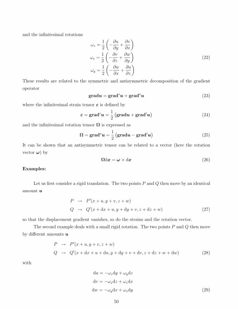
and the infinitesimal rotations

ωz =1

2

(−∂u

∂y+

∂v

∂x

)

ωx =1

2

(−∂v

∂z+

∂w

∂y

)(22)

ωy =1

2

(−∂w

∂x+

∂u

∂z

)

These results are related to the symmetric and antisymmetric decomposition of the gradient

operator

gradu = gradsu + gradau (23)

where the infinitesimal strain tensor ε is defined by

ε = gradsu =1

2

(gradu + gradtu

)(24)

and the infinitesimal rotation tensor Ω is expressed as

Ω = gradau =1

2

(gradu− gradtu

)(25)

It can be shown that an antisymmetric tensor can be related to a vector (here the rotation

vector ω) by

Ωdx = ω × dx (26)

Examples:

Let us first consider a rigid translation. The two points P and Q then move by an identical

amount u

P → P ′(x + u, y + v, z + w)

Q → Q′(x + dx + u, y + dy + v, z + dz + w) (27)

so that the displacement gradient vanishes, so do the strains and the rotation vector.

The second example deals with a small rigid rotation. The two points P and Q then move

by different amounts u

P → P ′(x + u, y + v, z + w)

Q → Q′(x + dx + u + du, y + dy + v + dv, z + dz + w + dw) (28)

with

du = −ωzdy + ωydz

dv = −ωxdz + ωzdx

dw = −ωydx + ωxdy (29)

50

so that the displacement gradient has only an antisymmetric part (i.e., ωx, ωy, ωz are the com-

ponents of the rotation vector ω), and the strains are vanishing.

The third case is such that

du = adx

dv = bdy

dw = cdz (30)

The displacement gradient is symmetric (i.e., no rotation occurs). The strain tensor has non

vanishing components associated to normal strains

εxx = a , εyy = b , εzz = c. (31)

7.2 Finite transformation strains

The aim of this part is to introduce the finite strains as an extension of the previous approach.

The more difficult aspects will be discussed in the next part. Let us consider again a point

P (x, y, z) experiencing a displacement u

P → P ′(x + u, y + v, z + w) (32)

and a second point Q(x + dx, y + dy, z + dz) in the vicinity of P moves to Q′

Q → Q′(x + dx + u + du, y + dy + v + dv, z + dz + w + dw). (33)

The theory of finite strain considers the length variation of a line joining the two considered

points in a reference state (dl = PQ) and in a deformed state (dl′ = P ′Q′)

(dl)2 = dx2 + dy2 + dz2

(dl′)2 = (dx + du)2 + (dy + dv)2 + (dz + dw)2. (34)

As a first approximation, Eqn. (18) is still used, and the length ratio becomes

(dl′

dl

)2

=

(dx

dl+

du

dl

)2

+

(dy

dl+

dv

dl

)2

+

(dz

dl+

dw

dl

)2

. (35)

By noting that

du

dl=

∂u

∂x

dx

dl+

∂u

∂y

dy

dl+

∂u

∂z

dz

dldv

dl=

∂v

∂x

dx

dl+

∂v

∂y

dy

dl+

∂v

∂z

dz

dl(36)

dw

dl=

∂w

∂x

dx

dl+

∂w

∂y

dy

dl+

∂w

∂z

dz

dl,

51

Eqn. (35) can be rewritten as

(dl′

dl

)2

=

(dx

dl+

∂u

∂x

dx

dl+

∂u

∂y

dy

dl+

∂u

∂z

dz

dl

)2

+

(dy

dl+

∂v

∂x

dx

dl+

∂v

∂y

dy

dl+

∂v

∂z

dz

dl

)2

(37)

+

(dz

dl+

∂w

∂x

dx

dl+

∂w

∂y

dy

dl+

∂w

∂z

dz

dl

)2

.

The strains are expressed with respect to a reference state that is undeformed. Let a, b and c

denote the cosine directors of dl

a =dx

dl, b =

dy

dl, c =

dz

dl, (38)

so that, by definition

(dl′

dl

)2

= (1 + 2Exx)a2 + (1 + 2Eyy)b

2 + (1 + 2Ezz)c2

+ 4Exyab + 4Eyzbc + 4Ezxca, (39)

with the normal strains

Exx =∂u

∂x+

1

2

[(∂u

∂x

)2

+

(∂u

∂y

)2

+

(∂u

∂z

)2]

Eyy =∂v

∂y+

1

2

[(∂v

∂x

)2

+

(∂v

∂y

)2

+

(∂v

∂z

)2]

(40)

Ezz =∂w

∂z+

1

2

[(∂w

∂x

)2

+

(∂w

∂y

)2

+

(∂w

∂z

)2]

and the shear strains

Exy = eyx =1

2

(∂u

∂y+

∂v

∂x+

∂u

∂x

∂u

∂y+

∂v

∂x

∂v

∂y+

∂w

∂x

∂w

∂y

)

Eyz = ezy =1

2

(∂v

∂z+

∂w

∂y+

∂u

∂y

∂u

∂z+

∂v

∂y

∂v

∂z+

∂w

∂y

∂w

∂z

)(41)

Ezx = exz =1

2

(∂w

∂x+

∂u

∂z+

∂u

∂z

∂u

∂x+

∂v

∂z

∂v

∂x+

∂w

∂z

∂w

∂x

)

corresponding to the Green-Lagrange strain tensor E

E =1

2

(gradu + gradtu + gradtu gradu

)(42)

52

The normal strains can be interpreted as

Exx =1

2

[(dx′

dx

)2

− 1

]=

1

2

[(1 + µx)

2 − 1]

Eyy =1

2

[(dy′

dy

)2

− 1

]=

1

2

[(1 + µy)

2 − 1]

(43)

Ezz =1

2

[(dz′

dz

)2

− 1

]=

1

2

[(1 + µx)

2 − 1],

where µx, µy, µz are the relative length variations (dx′ − dx)/dx, (dy′ − dy)/dy, (dz′ − dz)/dz,

respectively. Similarly, the shear strains are related to angle variations

2Exy =√

1 + 2Exx

√1 + 2Eyy cos θxy

2Eyz =√

1 + 2Eyy

√1 + 2Ezz cos θyz (44)

2Ezx =√

1 + 2Ezz

√1 + 2Exx cos θzx,

where θxy, θyz, θzx are the distortions of the vectors dy′ wrt. dx′, dz′ wrt. dy′, dx′ wrt. dz′,

respectively. (It is worth remembering that dx.dy = 0, dy.dz = 0, and dz.dx = 0.)

By noting that

−1 ≤ µx, µy, µz ≤ +∞ , −π/2 ≤ θxy, θyz, θzx ≤ π/2 (45)

the following bounds can be obtained for the components of the Green-Lagrange strain com-

ponents

−1/2 ≤ Exx, Eyy, Ezz ≤ +∞ , −1/2 ≤ Exy, Eyz, Ezx ≤ 1/2. (46)

7.3 Large transformation kinematics

Let us consider two neighboring points P and Q of a body Ω in its reference state, and a

corresponding frame R0. If a rigid body motion is applied, it corresponds to an isometry,

namely the distance between the points P ′ and Q′ after the transformation characterized by a

tensor A

P 0Q0 = A PQ (47)

is identical to the initial one

‖P 0Q0‖2 = PQ At A PQ = ‖PQ‖2, (48)

so that

AtA = I2 (49)

53

where I2 is the second order unit tensor. The first order derivative of the vector P 0Q0 is

expressed asdP 0Q0

dt= V (Q′/R0)− V (P ′/R0) (50)

or equivalentlydP 0Q0

dt= A At P 0Q0 (51)

where the tensor AAt is antisymmetric. As shown above, an antisymmetric tensor acting on

a vector can also be written as the cross product of a vector, here the rotation vector ω of Ω

with respect to R0, with P 0Q0

dP 0Q0

dt= ω(Ω/R0)× P 0Q0. (52)

Consequently, the vector field associated to a rigid body kinematics is such that

V (Q′/R0) = V (P ′/R0) + ω(Ω/R0)× P 0Q0 (53)

The motion of a body Ω is described by the function x0 = x0(x, t) giving the position

x0 at a time t of a particle that occupied the position x prior to a deformation. At a fixed

time, this function defines the deformation of the body between its reference configuration Cand the current one C ′. In Solid Mechanics, one chooses as reference configuration, the initial

configuration C and the current configuration in the same frame. It is however preferable,

to avoid any confusion, to distinguish these two frames, and in particular the Lagrangian

coordinates x for C and the Eulerian coordinates x′ for C ′. For the sake of simplicity, the two

systems are chosen orthogonal and normalized. As performed above, it is common to introduce

the displacement vector u(x, t)

x′(x, t) = x + u(x, t) (54)

Contrary to infinitesimal motions, no particular hypotheses are made concerning u. The func-

tion x′(x, t) defines the global motion of the body. Locally, i.e., for two points P and Q

separated by dx, one uses the deformation gradient tensor F relating an infinitesimal vector

dx in the reference configuration (C) to dx′ in the deformed configuration (C ′)

dx′ = F dx (55)

so that the tensor F can be related to the displacement gradient ∇u by

F = I2 + ∇u. (56)

The deformation gradient tensor defines the local motion. To measure a strain, i.e., a shape

change, it is necessary to eliminate the rotation. To characterize shape changes, one needs to

54

determine length variations as well as angle variations. In both cases, the information is given

by scalar products. Let us form the scalar product of dx′ with itself

dx′.dx′ = dx.F t F .dx (57)

where C = F t F denotes the right Cauchy-Green strain tensor. The Lagrangian strain measures

are formed by using C. It is possible to define various strain measures. The use of one rather

than another is a matter of choice or convenience. The only requirements are:

• they vanish for any rigid body motion (i.e., C = I2 for any rigid body motion),

• usually, they are positive for an expansion and negative for a contraction.

For Lagrangian measures, they can be expressed by using the strain tensors Em [32]

Em =

12m

(Cm − 1) when m 6= 0

12ln (C) when m → 0+

(58)

When m = 1, the Green-Lagrange strain tensor is obtained (see Section 7.2), m = 1/2 is the

Cauchy-Biot (or nominal) strain tensor and yields ∆L/L0 for a uniaxial elongation, where L0

is a reference (or gauge) length and ∆L the length variation. The case m → 0+ corresponds to

the logarithmic (or Hencky) strain tensor. The latter is the only additive strain measure. By

definition, all these strains are equal to zero for a rigid translation (i.e., F = I2 and C = I2)

or a rigid rotation (i.e., F = R and C = I2), where R is an orthogonal tensor. When the

amplitude of the body motion is small as well as the strain gradient, all measures converge

towards the infinitesimal strain tensor ε defined by

ε =1

2

[∇u + (∇u)t]. (59)

55

Correli Q4: A software for-finite-element-displacement field measurements by digital image correlation

Documents