Correlation model for spatially distributed ground …bakerjw/Publications/Jayaram_Baker_(2009...The estimated correlation model is also compared with previously published results,

EARTHQUAKE ENGINEERING AND STRUCTURAL DYNAMICSEarthquake Engng Struct. Dyn. 2009; 38:1687–1708Published online 28 April 2009 in Wiley InterScience (www.interscience.wiley.com). DOI: 10.1002/eqe.922

Correlation model for spatially distributedground-motion intensities

Nirmal Jayaram∗,† and Jack W. Baker

Department of Civil and Environmental Engineering, Stanford University, Stanford, CA 94305-4020, U.S.A.

SUMMARY

Risk assessment of spatially distributed building portfolios or infrastructure systems requires quantificationof the joint occurrence of ground-motion intensities at several sites, during the same earthquake. Theground-motion models that are used for site-specific hazard analysis do not provide information on thespatial correlation between ground-motion intensities, which is required for the joint prediction of intensitiesat multiple sites. Moreover, researchers who have previously computed these correlations using observedground-motion recordings differ in their estimates of spatial correlation. In this paper, ground motionsobserved during seven past earthquakes are used to estimate correlations between spatially distributedspectral accelerations at various spectral periods. Geostatistical tools are used to quantify and expressthe observed correlations in a standard format. The estimated correlation model is also compared withpreviously published results, and apparent discrepancies among the previous results are explained.

The analysis shows that the spatial correlation reduces with increasing separation between the sites ofinterest. The rate of decay of correlation typically decreases with increasing spectral acceleration period. Atperiods longer than 2 s, the correlations were similar for all the earthquake ground motions considered. Atshorter periods, however, the correlations were found to be related to the local-site conditions (as indicatedby site Vs30 values) at the ground-motion recording stations. The research work also investigates theassumption of isotropy used in developing the spatial correlation models. It is seen using the Northridgeand Chi-Chi earthquake time histories that the isotropy assumption is reasonable at both long and shortperiods. Based on the factors identified as influencing the spatial correlation, a model is developed thatcan be used to select appropriate correlation estimates for use in practical risk assessment problems.Copyright q 2009 John Wiley & Sons, Ltd.

Received 6 October 2008; Revised 11 March 2009; Accepted 17 March 2009

KEY WORDS: spatial correlation; spectral accelerations; coherency; risk assessment; infrastructuresystems

∗Correspondence to: Nirmal Jayaram, Department of Civil and Environmental Engineering, Stanford University,Stanford, CA 94305-4020, U.S.A.

†E-mail: [email protected]

Contract/grant sponsor: U.S. Geological Survey (USGS); contract/grant number: 07HQGR0031

Copyright q 2009 John Wiley & Sons, Ltd.

1688 N. JAYARAM AND J. W. BAKER

1. INTRODUCTION

The probabilistic assessment of ground-motion intensity measures (such as spectral acceleration) atan individual site is a well researched topic. Several ground-motion models have been developed topredict median ground-motion intensities as well as dispersion about the median values e.g. [1–4].Site-specific hazard analysis does not suffice, however, in many applications that require knowledgeabout the joint occurrence of ground-motion intensities at several sites, during the same earthquake.For instance, the risk assessment of portfolios of buildings or spatially distributed infrastructuresystems (such as transportation networks, oil and water pipeline networks and power systems)requires the prediction of ground-motion intensities at multiple sites. Such joint predictions arepossible, however, only if the correlation between ground-motion intensities at different sites areknown e.g. [5, 6]. The correlation is known to be large when the sites are close to one another,and decays with increase in separation between the sites. Park et al. [7] report that ignoring orunderestimating these correlations overestimates frequent losses and underestimates rare ones,and hence, it is important that accurate ground-motion correlation models be developed for lossassessment purposes. The current work analyzes correlations between the ground-motion intensitiesobserved in recorded ground motions, in order to identify factors that affect these correlationsand to select a correlation model that can be used for the joint prediction of spatially distributedground-motion intensities in future earthquakes.

Ground-motion models that predict intensities at an individual site i due to an earthquake jtake the following form:

ln(Yi j )= ln(Yi j )+�i j +� j (1)

where Yi j denotes the ground-motion parameter of interest (e.g. Sa(T ), the spectral acceleration atperiod T ); Yi j denotes the predicted (by the ground-motion model) median ground-motion intensity(which depends on parameters such as magnitude, distance, period and local-site conditions); �i jdenotes the intra-event residual, which is a random variable with zero mean and standard deviation�i j ; and � j denotes the inter-event residual, which is a random variable with zero mean and standarddeviation � j . The standard deviations, �i j and � j , are estimated as a part of the ground-motionmodel and are a function of the spectral period of interest, and in some models also as a functionof the earthquake magnitude and the distance of the site from the rupture. During an earthquake,the inter-event residual (� j ) computed at any particular period is a constant across all the sites.

Jayaram and Baker [8] showed that a vector of spatially distributed intra-event residualse j =(�1 j ,�2 j , . . . ,�d j ) follows a multivariate normal distribution. Hence, the distribution of e j canbe completely defined using the first two moments of the distribution, namely, the mean andvariance of e j , and the correlation between all �i1 j and �i2 j pairs. (Alternately, the distributioncan be defined using the mean and the covariance of e j , since the covariance completely specifiesthe variance and correlations.) Since the intra-event residuals are zero-mean random variables, themean of e j is the zero vector of dimension d . The covariance, however, is not entirely knownfrom the ground-motion models since the models only provide the variances of the residuals andnot the correlation between residuals at two different sites.

Researchers, in the past, have computed these correlations using ground-motion time historiesrecorded during earthquakes [9–11]. Boore et al. [11] used the observations of peak groundacceleration (PGA, which equals Sa(0)) from the 1994 Northridge earthquake to compute thespatial correlations. Wang and Takada [10] computed the correlations using the observations ofpeak ground velocities (PGV) from several earthquakes in Japan and the 1999 Chi-Chi earthquake.

Copyright q 2009 John Wiley & Sons, Ltd. Earthquake Engng Struct. Dyn. 2009; 38:1687–1708DOI: 10.1002/eqe

SPATIALLY DISTRIBUTED GROUND-MOTION INTENSITIES 1689

Goda and Hong [9] used the Northridge and Chi-Chi earthquake ground-motion records to computethe correlation between PGA residuals, as well as the correlation between residuals computedfrom spectral accelerations at three periods between 0.3 and 3 s. The results reported by theseresearch works, however, differ in terms of the rate of decay of correlation with separation distance.For instance, while Boore et al. [11] report that the correlation drops to zero at a site separationdistance of approximately 10 km, the non-zero correlations observed by Wang and Takada [10]extend past 100 km. Further, Goda and Hong [9] observe the differences between the correlationdecay rate estimated using the Northridge earthquake records and the correlation decay rate basedon the Chi-Chi earthquake records. To date, no explanation for these differences has been identified.

The current work uses observed ground motions to estimate correlations between ground-motion intensities (in particular, spectral accelerations). Factors that affect the rate of decay in thecorrelation with separation distance are identified. The work also provides probable explanationsfor the differing results reported in the literature. In this study, an emphasis is placed on developinga standard correlation model that can be used for predicting spatially distributed ground-motionintensities for risk assessment purposes.

2. MODELING CORRELATIONS USING SEMIVARIOGRAMS

Geostatistical tools are widely used in several fields for modeling spatially distributed randomvectors (also called random functions) [12, 13]. The current research work takes advantage ofthis well-developed approach to model the correlation between spatially distributed ground-motionintensities. The needed tools are briefly described in this section.

Let Z=(Zu1, Zu2, . . . , Zud ) denote a spatially distributed random function, where ui denotes thelocation of the site i ; Zui is the random variable of interest (in this case, �ui j from Equation (1))at site location ui and d denotes the total number of sites. The correlation structure of the randomfunction Z can be represented by a semivariogram, which is a measure of the average dissimilaritybetween the data [13]. Let u and u′ denote the two sites separated by h. The semivariogram(�(u,u′)) is computed as half the expected squared difference between Zu and Zu′ .

�(u,u′)= 12 [E{Zu−Zu′ }2] (2)

The semivariogram defined in Equation (2) is location-dependent and its inference requiresrepetitive realizations of Z at locations u and u′. Such repetitive measurements of {Zu, Zu′ } are,however, never available in practice (e.g. in the current application, one would need repeatedobservations of ground motions at every pair of sites of interest). Hence, it is typically assumedthat the semivariogram does not depend on site locations u and u′, but only on their separation h.The stationary semivariogram (�(h)) can then be obtained as follows:

�(h)= 12 [E{Zu−Zu+h}2] (3)

Equation (2) can be replaced with Equation (3) if the random function (Z) is second-orderstationary. Second-order stationarity implies that (i) the expected value of the random variable Zuis a constant across space and (ii) the two-point statistics (measures that depend on Zu and Zu′)depend only on the separation between u and u′, and not on the actual locations (i.e. the statisticsdepend on the separation vector h between u and u′ and not on u and u′ as such). A stationary



semivariogram can be estimated from a data set as follows:

�(h)= 1

2N (h)

N (h)∑�=1

{zu� −zu�+h}2 (4)

where �(h) is the experimental stationary semivariogram (estimated from a data set); zu denotes thedata value at location u; N (h) denotes the number of pairs of sites separated by h; and {zu�, zu�+h}denotes the �th such pair. A stationary semivariogram is said to be isotropic if it is a function ofthe separation distance (h=‖h‖) rather than the separation vector h.

The function �(h) provides a set of experimental values for a finite number of separationvectors h. A continuous function must be fitted based on these experimental values in order todeduce semivariogram values for any possible separation h. A valid (permissible) semivariogramfunction needs to be negative definite so that the variances and conditional variances correspondingto this semivariogram are non-negative. In order to satisfy this condition, the semivariogramfunctions are usually chosen to be the linear combinations of basic models that are known to bepermissible. These include the exponential model, the Gaussian model, the spherical model andthe nugget effect model.

The exponential model, in an isotropic case (i.e. the vector distance h is replaced by a scalarseparation length ‖h‖, also denoted as h), is expressed as follows:

�(h)=a[1−exp(−3h/b)] (5)

where a and b are the sill and the range of the semivariogram function, respectively (Figure 1(a)).The sill of a semivariogram equals the variance of Zu , while the range is defined as the separationdistance h at which �(h) equals 0.95 times the sill of the exponential semivariogram.

The Gaussian model is as follows:

�(h)=a[1−exp(−3h2/b2)] (6)

The sill and the range of a Gaussian semivariogram are as defined for an exponential semivariogram.

Figure 1. (a) Parameters of a semivariogram and (b) Semivariograms fitted to the same data set using themanual approach and the method of least squares.



The spherical model is as follows:

�(h) =a

[3

2

(h

b

)− 1

2

(h

b

)3]

if h�b

=a otherwise (7)

where a and b are again the sill and range of the semivariogram, respectively. The range of aspherical semivariogram is the separation distance at which �(h) equals a.

The nugget effect model can be described as:

�(h)=a[I (h>0)] (8)

where I (h>0) is an indicator variable that equals 1 when h>0 and equals 0 otherwise.The covariance structure of Z is completely specified by the semivariogram function and the sill

and the range of the semivariogram. It can be theoretically shown that the following relationshipholds [13]:

�(h)=a(1−�(h)) (9)

where �(h) denotes the correlation coefficient between Zu and Zu+h . It can also be shown thatthe sill of the semivariogram equals the variance of Zu . Therefore, it would suffice to estimatethe semivariogram of a random function in order to determine its covariance structure. Moreover,based on Equations (5) (for instance) and (9), it can be seen that a large range implies a smallrate of increase in �(h) and therefore, large correlations between Zu and Zu+h . Further, it canbe seen from Equation (8) that the nugget effect model specifies zero correlation for all non-zeroseparation distances.

In the current work, correlations between ground-motion intensities at different sites are repre-sented using semivariograms. Ground-motion recordings from past earthquakes are used to estimateranges of semivariograms and to identify the factors that could affect the estimates. Throughoutthis work, the semivariograms are assumed to be second-order stationary. Second-order station-arity is assumed so that the data available over the entire region of interest can be pooled andused for estimating semivariogram sills and ranges. In the current work, like many other worksinvolving spatial correlation estimation, the semivariograms are also assumed to be isotropic. Theassumptions of stationarity and isotropy are investigated in more detail subsequently in this paper.

3. COMPUTATION OF SEMIVARIOGRAM RANGES FOR INTRA-EVENT RESIDUALSUSING EMPIRICAL DATA

As mentioned earlier, the covariance of intra-event residuals can be represented using a semivari-ogram, whose functional form (e.g. exponential model), sill and range need to be determined. Thissection discusses the semivariograms estimated based on observed ground-motion time histories.

For a given earthquake, it can be seen from Equation (1) that

�i +�= ln(Yi )− ln(Yi ) (10)



Let �i denote the normalized intra-event residual at site i . (The subscript j in Equation (1) is nolonger used since the residuals used in these calculations are observed during a single earthquake.)�i is computed as follows:

�i = �i�i

(11)

where �i denotes the standard deviation of the intra-event residual at site i . Further, let �i denotethe sum of the intra-event residual (�i ) and inter-event residual (�) normalized by the standarddeviation of the intra-event residual (�i ). �i can be computed as follows:

�i = �i +�

�i= ln(Yi )− ln(Yi )

�i(12)

While assessing covariances, it is convenient to work with �’s rather than �’s, since �’s arehomoscedastic (i.e. constant variance) with unit variance unlike the �’s.

Since the inter-event residual (�), computed at any particular period, is a constant across all thesites during a given earthquake, the experimental semivariogram function of � can be obtained asfollows (based on Equation (4)):

�(h) = 1

2N (h)

N (h)∑�=1

[�u� − �u�+h]2

= 1

2N (h)

N (h)∑�=1

[ln(Yu�)− ln(Yu�)−�

�u�

− ln(Yu�+h)− ln(Yu�+h)−�

�u�+h

]2

≈ 1

2N (h)

N (h)∑�=1

[ln(Yu�)− ln(Yu�)

�u�

− ln(Yu�+h)− ln(Yu�+h)

�u�+h

]2

= 1

2N (h)

N (h)∑�=1

[�u� − �u�+h]2 (13)

where � is defined by Equation (12); (u�,u�+h) denotes the location of a pair of sites separatedby h; N (h) denotes the number of such pairs; Yu� denotes the ground-motion intensity at locationu�; and �u� is the standard deviation of the intra-event residual at location u�. The sill of thesemivariogram of � (i.e. the sill of �(h)) should equal 1 since the �’s have a unit variance. Hence,based on Equation (9), it can be concluded that

�(h)=1− �(h) (14)

where �(h) is the estimate of �(h).Incidentally, Equation (13) shows that the covariances of intra-event residuals can be estimated

without having to account for the inter-event residual �. As indicated, Equation (13) involves anapproximation due to the mild assumption that �/�u� =�/�u�+h . The Boore and Atkinson [1]model, which is used in the current work, suggests that the standard deviation of the intra-eventresiduals depends only on the period at which the residuals are computed, and hence, it can beinferred that this approximation is reasonable. Incidentally, though the current work only uses theBoore and Atkinson [1] ground-motion model, the results obtained were found to be similar whenan alternate model, namely, the Chiou and Youngs [3] model, was used.



The ground-motion databases typically report recordings in two orthogonal horizontal direc-tions. For instance, the PEER NGA database [14] provides the fault-normal and the fault-parallelcomponents of the ground motions for each earthquake. In the current work, it was found that thecorrelations computed using both the fault-normal and the fault-parallel time histories were similar.Hence, only results corresponding to the fault-normal orientation are reported here. In fact, Bakerand Jayaram [15] and Bazzurro et al. [16] used several sets of recorded and simulated groundmotions to show that the estimated correlations are independent of the ground-motion componentused.

3.1. Construction of experimental semivariograms using empirical data

Figure 1(a) shows a sample semivariogram constructed from empirical data. The first step inobtaining such a semivariogram is to compute site-to-site distances for all pairs of sites and placethem in different bins based on the separation distances. For example, the bins could be centered atmultiples of h km with bin widths of h km (h�h). All pairs of sites that fall in the bin centeredat h km (i.e. the sites that are separated by a distance ∈(h−h/2,h+h/2) are used to compute�(h) (based on Equation (4)). If h is chosen to be very small, it can result in few pairs of sitesin the bins, which will affect the robustness of the results obtained. On the other hand, a largevalue of h will mix site pairs with differing distances reducing the resolution of the experimentalsemivariograms. In the current work, experimental semivariograms are obtained using h=2km(unless stated otherwise), since this was seen to be the smallest value that results in a reasonablenumber of site pairs in the bins.

The semivariogram shown in Figure 1(a) has an exponential form with a sill of 1 and a rangeof 40 km. This model can be expressed as follows (based on Equation (5)):

�(h)=1−exp(−3h/40) (15)

The correlation function corresponding to this model equals �(h)=1−�(h)=exp(−3h/40) (basedon Equation (14)).

An easy and transparent method to determine the model and the model parameters is to fit theexperimental semivariogram values obtained at discrete separation distances manually. Supposethat �(h) can be expressed as follows:

�(h)=c0�0(h)+N∑

n=1cn�n(h) (16)

where �0(h) is a pure nugget effect and �n(h) is a spherical, exponential or Gaussian model (asdefined in Equations (5)–(8)); cn is the contribution of the model n to the semivariogram; and Nis the total number of models used (excluding the nugget effect). The ranges and the contributionsof the models can be systematically varied to obtain the best fit to the experimental semivariogramvalues.

In the following sections, priority is placed on building models that fit the empirical data well atshort distances, even if this requires some misfit with empirical data at large separation distances,because it is more important to model the semivariogram structure well at short separation distances.This is because the large separation distances are associated with low correlations, which thus haverelatively a little effect on joint distributions of ground-motion intensities. In addition to havinglow correlation, widely separated sites also have a little impact on each other due to an effective‘shielding’ of their influence by more closely-located sites [13]. Figure 1(b) shows the sample



Figure 2. Range of semivariograms of �, as a function of the period at which � values are computed:(a) the residuals are obtained using the Northridge earthquake data and (b) the residuals are obtained

using the Chi-Chi earthquake data.

semivariograms fitted to a data set using the manual approach and the method of least squares. Itcan be seen that, at small separations, the manually fitted semivariogram is a better model than theone fitted using the method of least squares. More detailed discussion on the advantages of usingmanual-fitting rather than least-squares fitting follows in Section 5, where the proposed approachis also compared with approaches used in previous research on this topic.

3.2. 1994 Northridge earthquake recordings

This section discusses the ranges of semivariograms estimated using observed Northridge earth-quake ground motions. The manual fitting approach described previously is used to computeranges of the semivariograms of �’s (obtained based on the Northridge earthquake time histories)computed at seven periods ranging between 0 and 10 s. Of the three functional forms consid-ered (Equations (5)–(7)), the exponential model is found to provide the ‘best fit’ (particularlyat small separations) for experimental semivariograms obtained using �’s computed at severaldifferent periods, based on recordings from different earthquakes. The constancy of the semivar-iogram function across periods makes it simpler to specify a standard correlation model for the�’s. Moreover, the use of a single model enables a direct comparison of the correlations betweenresiduals computed at different periods, using only the ranges of the semivariograms. The rangesof these estimated semivariograms are plotted against period in Figure 2(a). The semivariogramfits corresponding to all the periods considered can be found in Baker and Jayaram [15].

It can be observed from Figure 2(a) that the estimated range of the semivariogram tends toincrease with period. As described earlier, it can be inferred that the � values at long periods showlarger correlations than those at short periods. This is consistent with comparable past studiesof ground-motion coherency, which has been widely researched in the past. Coherency can bethought of as a measure of similarity in two spatially separated ground-motion time histories. DerKiureghian [17] reports that coherency is reduced by the scattering of waves during propagation,and that this reduction is greater for high-frequency waves. High-frequency waves, which haveshort wavelengths, tend to be more affected by small-scale heterogeneities in the propagation path,and as a result tend to be less coherent than long period ground waves [18]. It is reasonable to expecthighly coherent ground motions to exhibit correlated peak amplitudes (i.e. spectral accelerations)as well. Since the �’s studied here, which quantify these peak amplitudes, tend to show the same



correlation trend with period as previous coherency studies, it may be that a similar wave scatteringmechanism is partially responsible for the correlation trends observed here.

The Northridge earthquake data used for the above analysis are obtained from the NGA database.In order to exclude records whose characteristics differ from those used by the ground-motionmodelers for data analysis, in most cases, only records used by the authors of the Boore andAtkinson [1] ground-motion model are considered. For the purposes of this paper, these recordsare denoted as ‘usable records’. The semivariograms of residuals computed at periods of 5, 7.5 and10 s, however, are obtained using all available Northridge records in the NGA database. This ison account of the limited number of Northridge earthquake recordings at extremely long periods.At 5 s the residuals can be computed using 158 total available records, while 66 of these are usedby the ground-motion model authors. Since there is a reasonable number of records available inboth cases, a semivariogram constructed using all 158 records (denoted SV1) can be comparedwith that estimated from the usable 66 records (in this case, the bin size was increased to 4 km tocompensate for the lack of available records) (denoted SV2). The ranges of the two semivariograms,SV1 and SV2, are 40 and 30 km, respectively. This shows that there is a slight difference in theestimated ranges, which could be due to the additional correlated systematic errors introduced bythe extra records.

As mentioned in Section 1, correlation between intensities estimated using the fault-normalcomponents are discussed in this paper. This is because the correlations obtained using the fault-normal and the fault-parallel ground motions were found to be similar. For example, the semi-variogram of �’s computed at 2 s, based on the fault-parallel ground motions recorded during theNorthridge earthquake was found to be reasonably modeled using an exponential function witha unit sill and a range of 36 km. The corresponding range for the semivariogram based on thefault-normal ground motions equals 42 km. Similar results were observed when the residuals werecomputed at other periods, and using other earthquake recordings.

3.3. 1999 Chi-Chi earthquake

In this section, the semivariogram ranges of �’s from the Chi-Chi earthquake recordings arepresented. The Chi-Chi earthquake ground motions came from the NGA database. Only recordsused by Boore and Atkinson [1] ground-motion model are considered. The summary plot of theestimated ranges is shown in Figure 2(b). The following can be observed from the figures:

(a) As seen with the Northridge earthquake data, the range of the semivariogram typicallyincreases with period (An exception is observed when the PGA’s are considered, and thisis explored further subsequently in this paper.).

(b) The ranges are higher, in general, than those observed based on the Northridge earthquakedata (Figure 2(a)). This is consistent with observations made by other researchers consideringNorthridge and Chi-Chi earthquake data e.g. [9].

The large ranges obtained here, relative to the comparable results from Northridge, can beexplained using the Vs30 values (average shear-wave velocities in the top 30m of the soil) at therecording stations. The Vs30 values are commonly used in ground-motion models as indicatorsof the effects of local-site conditions on the ground motion. �′s are affected if the predictedground-motion intensities are affected by inaccurate Vs30 values, or if the Vs30’s are inadequateto capture the local-site effects adequately (i.e. the ground-motion models do not entirely capturethe local-site effects using Vs30 values).



Close to 70% of the Taiwan site Vs30 values are inferred from Geomatrix site classes, whilethe rest of the Vs30 values are measured (NGA database). Since closely spaced sites are likely tobelong to the same site class and posess similar (and unknown) Vs30 values, errors in the inferredVs30 values are likely to be correlated among sites that are close to each other. Such correlatedVs30 measurement errors will result in correlated prediction errors at all these closely spaced sites,which will increase the range of the semivariograms.

The larger ranges of semivariograms estimated using the Chi-Chi earthquake ground motionsmay also be due to possible correlation between the true Vs30 values (and not just the correlationbetween the Vs30 errors). Larger correlation between the Vs30’s indicate a more homogeneoussoil (homogeneous in terms of properties that affect site effects but not accounted by the ground-motion models). In such cases, if a ground-motion model does not accurately capture the local-site effect at one site, it is likely to produce similar prediction errors in a cluster of closelyspaced sites (on account of the homogeneity). Castellaro et al. [19] compared the site-dependentseismic amplification factors (Fa , the site amplification factor is defined as the amplification ofthe ground-motion spectral level at a site with respect to that at a reference ground condition [20])observed during the 1989 Loma Prieta earthquake to the corresponding site Vs30 values. Theyfound substantial scatter in the plot of Fa versus Vs30, and also found that this scatter was morepronounced at short periods (below 0.5 s) than at longer periods. This suggests that ground-motionintensity predictions based on Vs30 will have errors, particularly at periods below 0.5 s.

Figures 3(a) and (b) show semivariograms of the normalized Vs30 values (the Vs30 semivar-iogram is not to be confused with the � semivariogram) at the Northridge earthquake recordingstations and the Chi-Chi earthquake recording stations, respectively (Normalization involvesscaling the Vs30 values so that the normalized Vs30 values have a unit variance to enable adirect comparison of the semivariograms.). Figure 3(a) shows significant scatter at all separationdistances indicating zero correlation at all separations. In contrast, Figure 3(b) indicates that theTaiwan Vs30 values have significant spatial correlation. This suggests that �’s may have additionalspatial correlation in Taiwan, due to homogeneous site effects that cause correlated predictionerrors.

As mentioned previously, one notable aberration in the plot of range versus period (Figure 2(b))is the large range observed when the residuals are computed at 0 s as compared with some of thelonger periods. This is not consistent with the coherency argument of the previous section. It can,however, be explained using the relationship between the range and the Vs30’s described in theabove paragraphs. The inaccuracies in ground-motion prediction based on Vs30’s will reflect inincreased correlation between the residuals computed at nearby sites. These inaccuracies are largerat short periods (below 0.5 s) [19], which explains the larger correlation between the residuals(which ultimately results in the larger range observed) computed using PGAs.

One final test that was considered here was whether spatial correlations differed for near-faultground motions experiencing directivity. Baker [21] identified pulse-like ground motions from theNGA database based on wavelet analysis. Thirty such pulses were identified in the fault-normalcomponents of the Chi-Chi earthquake recordings. Experimental semivariograms of residuals werecomputed using these pulse-like ground motions, and their ranges were estimated. It was seen thatthe ranges were reasonably similar to those obtained using all usable ground motions (i.e. pulse-likeand non-pulse-like). Since the available pulse-like ground-motion data set is very small, however,the results obtained were not considered to be sufficiently reliable, and hence not considered furtherin this paper. A more detailed analysis can be found in Baker and Jayaram [15] and Bazzurroet al. [16].



Figure 3. (a) Experimental semivariogram obtained using normalized Vs30’s at the recording stations of theNorthridge earthquake. No semivariogram is fitted on account of the extreme scatter and (b) experimentalsemivariogram obtained using normalized Vs30’s at the recording stations of the Chi-Chi earthquake. The

range of the fitted exponential semivariogram equals 25 km.

Based on the discussion in this section, it can be seen that the correlated Vs30 values and thecorrelated Vs30 measurement errors are the possible reasons for the larger ranges estimated inSection 3.3 than in Section 3.2. Other factors, such as the size of the rupture areas, may alsoaffect the correlations. These factors could not, however, be investigated with the limited data setavailable.

3.4. Other earthquakes

The correlations computed using data from the 2003 M5.4 Big Bear City earthquake, the 2004M6.0 Parkfield earthquake, the 2005 M5.1 Anza earthquake, the 2007 M5.6 Alum Rock earthquakeand the 2008 M5.4 Chino Hills earthquake are presented in this section. The time histories forthese earthquakes were obtained from the CESMD database [22]. The Vs30 data used for thesecomputations came from the CESMD database [22] (for the Parkfield earthquake) and the U.S.Geological Survey Vs30 maps (for the other earthquakes) [23].

Exponential models are fitted to experimental semivariograms of �’s computed using the timehistories from the above-mentioned earthquakes, at periods ranging from 0–10 s. Figure 4 showsplots of range versus period for the Big Bear City, Parkfield, Alum Rock, Anza and Chino Hillsearthquake residuals. The ranges of the semivariograms are generally seen to increase with period,which is consistent with findings from the Chi-Chi and the Northridge earthquake data. It can alsobe seen from the figure that, at short periods, the ranges obtained from the Anza earthquake data arelarger than those from the other earthquakes considered. On the other hand, the ranges computedusing the Parkfield earthquake data are fairly small at short periods. Semivariograms of the Vs30’sat the recording stations for all five earthquakes of interest were computed. The semivariogramrange computed using the Anza earthquake Vs30’s was found to be the largest at 40 km, whilethe ranges computed from the Chino Hills, Big Bear City, Alum Rock and Parkfield earthquakedata were smaller at 35, 30, 18 and approximately 0 km, respectively. The estimated ranges of thesemivariograms of the residuals and of the Vs30’s reinforce the argument made previously that



Figure 4. Range of semivariograms of �, as a function of the period at which � values are computed.The residuals are obtained using the: (a) Big Bear City earthquake data; (b) Parkfield earthquake data;

(c) Alum Rock earthquake data; (d) Anza earthquake data; and (e) Chino Hills earthquake data.

clustering in the Vs30 values (as indicated by a large range of the Vs30 semivariogram) results inincreased correlation among the residuals (the low PGA-based range estimated using the Chinohills earthquake data seems to be an exception, however). This trend is seen in Figure 5, whichshows the range of PGA-based residuals plotted against the range of the Vs30’s, for the earthquakesconsidered in this work. This dependence on the Vs30 range seems to be lesser at longer periods,which is in line with the observations of Castellaro et al. [19] that the scatter in the plot of Fa versus



Figure 5. Ranges of residuals computed using PGAs versus ranges of normalized Vs30 values.

Vs30 is greater at short periods than at long periods. The authors hypothesize that the reduceddependence of range on Vs30’s at long periods could also be because the long-period ranges areconsiderably influenced by factors other than Vs30 values, such as coherency as explained inSection 3.2 and prediction errors unrelated to Vs30’s (which are likely since the ground-motionmodels are fitted using much fewer data points at long periods). Finally, an additional advantageof considering these five additional events is that earthquakes covering a range of magnitudes havebeen studied. No trends of range with magnitude were detected.

A few research works studying spatial correlations use ground-motion recordings from earth-quakes in Japan, based on the data provided in the KiK Net [24]. In this work, data from the 2004Mid Niigata Prefecture earthquake and the 2005 Miyagi-Oki earthquake were explored. Thoughthe number of sites at which the ground-motion recordings are available is fairly large, mostrecording stations are far away from each another. The KiK Net [24] consists of 681 recordingstations, of which only 19 pairs of stations are within 10 km of one another. As explained inSection 3.2, it is important to accurately model the semivariogram at short separation distances,particularly at separation distances below 10 km. Hence, the recordings from the KiK Net [24]were not considered further for studying the ranges of semivariograms.

3.5. A predictive model for spatial correlations

The above sections presented the spatial correlations computed using recorded ground motionsfrom several past earthquakes. In this section, these correlation estimates are used to develop amodel that can be used to select appropriate correlation estimates for risk assessment purposes.

Figure 6(a) shows the ranges computed using various earthquake data as a function of period.From a practical perspective, despite the wide differences in the characteristics of the earthquakesconsidered, the ranges computed are quite similar, particularly at periods longer than 2 s. At shortperiods (below 2 s), however, there are considerable differences in the estimated ranges dependingon the ground-motion time histories used. The previous sections suggested empirically that the



0 2 4 6 8 100

10

20

30

40

50

60

70

80

90

100

Period (s)

Ran

ge (

km)

Anza earthquakeAlum Rock earthquakeParkfield earthquakeChi-Chi earthquakeNorthridge earthquakeBig Bear City earthquakeChino Hills earthquake

0 2 4 6 8 100

10

20

30

40

50

60

70

80

90

100

Period (s)

Ran

ge (

km)

Case 2Case 1

Cases 1 and 2

(a) (b)

Figure 6. (a) Range of semivariograms of �, as a function of the period at which � values are computed.The residuals are obtained from six different sets of time histories as shown in the figure and (b) range

of semivariograms of � predicted by the proposed model as a function of the period.

differences in correlation of �’s is in large part explained by the Vs30 values at the recordingstations for these earthquakes. Hence, the following cases can be considered for decision making:

Case 1: If the Vs30 values do not show or are not expected to show clustering (i.e. the geologiccondition of the soil varies widely over the region (this can also be quantified by constructing thesemivariogram of the Vs30’s as explained previously)), the smaller ranges reported in Figure 6(a)will be appropriate.

Case 2: If the Vs30 values show or are expected to show clustering (i.e. there are clusters of sitesin which the geologic conditions of the soil are similar), the larger ranges reported in Figure 6(a)should be chosen.

Based on these conclusions, the following model was developed to predict a suitable rangebased on the period of interest:At short periods (T<1 s), for case 1:

b=8.5+17.2T (17)

At short periods (T<1 s), for case 2:

b=40.7−15.0T (18)

At long periods (T�1 s), for both cases 1 and 2:

b=22.0+3.7T (19)

where b denotes the range of the exponential semivariograms (Equation (5)), and T denotes theperiod. Based on this model, the correlation between normalized intra-event residuals separatedby h km is obtained as follows (follows from Equations (5) and (14)):

�(h)=exp(−3h/b) (20)

It is to be noted that the correlations between intra-event residuals will exactly equal the correlationsbetween normalized intra-event residuals defined above.



The plot of the predicted range versus period is shown in Figure 6(b). The model has beendeveloped based on only seven earthquakes, but since the trends exhibited were found to besimilar for these seven, it can be expected that the model will predict reasonable ranges for futureearthquakes.

The predictive model can be used for simulating correlated ground-motion fields for a particularearthquake as follows:

Step 1: Obtain median ground-motion values (denoted Yi j in Equation (1)) at the sites of interestusing a ground-motion model.

Step 2: Probabilistically generate (simulate) the inter-event residual term (� j in Equation (1)),which follows a univariate normal distribution. The mean of the inter-event residual is zero, andits standard deviation can be obtained using ground-motion models.

Step 3: Simulate the intra-event residuals (�i j in Equation (1)) using the standard deviationsfrom the ground-motion models and the correlations from Equations (17)–(20).

Step 4: Combine the three terms generated in Steps 1–3 using Equation (1) to obtain simulatedground-motion intensifies at the sites of interest.

4. ISOTROPY OF SEMIVARIOGRAMS

This section examines the assumption of isotropy of semivariograms using the ground motionsdiscussed previously.

4.1. Isotropy of intra-event residuals

A stationary semivariogram (�(h)) is said to be isotropic if it depends only on the separationdistance h=‖h‖, rather than the separation vector h. Anisotropy is said to be present when thesemivariogram is also influenced by the orientation of the data locations. The presence of anisotropycan be studied using directional semivariograms [13]. Directional semivariograms are obtainedas shown in Equation (4) except that the estimate is obtained using only pairs of (zu�, zu�+h)

such that the azimuth of the vector h are identical and as specified for all the pairs. Since anisotropic semivariogram is independent of data orientation, the directional semivariograms obtainedconsidering any specific azimuth will be identical to the isotropic semivariogram if the data arein fact isotropic. Differences between the directional semivariograms indicate one of two differentforms of anisotropy, namely, geometric anisotropy and zonal anisotropy. Geometric anisotropy issaid to be present if directional semivariograms with differing azimuths have differing ranges.Zonal anisotropy is indicated by a variation in the sill with azimuth.

4.2. Construction of a directional semivariogram

A directional semivariogram is specified by several parameters, as illustrated in Figure 7(a).The parameters include the azimuth of the direction vector (the azimuth angle () is measuredfrom the North), the azimuth tolerance (), the bin separation (h) and the bin width (h).A semivariogram obtained using all pairs of points irrespective of the azimuth is known as theomni-directional semivariogram, and is an accurate measure of spatial correlation in the presenceof isotropy. (The semivariograms that have been described in the previous sections are omni-directional semivariograms.) In determining the experimental semivariogram in any bin, only pairsof sites separated by distance ranging between [h−h/2,h+h/2], and with azimuths ranging



between [−,+] are considered. For example, let � be a site located in a two-dimensionalregion, as shown in Figure 7(a). It is intended to construct a directional semivariogram with anazimuth of (as marked in the figure). The computation of the experimental semivariogram value(�(h)) involves pairing up the data values at all sites falling within the hatched region (the regionthat satisfies the conditions on the separation distance and the azimuth, as mentioned above) withthe data values at site � (i.e. u�). The area of the hatched region is defined by the azimuth toleranceused and can be seen to increase with increase in separation distance (h) (Figure 7(a)). For largevalues of h, the area of the hatched region will be undesirably large and hence, in addition toplacing constraints on the azimuth tolerance, a constraint is explicitly specified on the bandwidthof the region of interest, as marked in the figure.

It is usually difficult to compute experimental directional semivariograms on account of theneed to obtain pairs of sites oriented along pre-specified directions. Hence, it is required thatthe bin width, the azimuth tolerance and the bandwidth be specified liberally while constructingdirectional semivariograms. The results reported in this paper are obtained by considering a binseparation of 4 km, a bin width of 4 km, an azimuth tolerance of 10◦ and a bandwidth of 10 km.Directional semivariograms are plotted for azimuths of 0, 45 and 90◦ in order to capture the effectsof anisotropy, if any.

4.3. Test for anisotropy using Northridge ground-motion data

Figure 7(b–d) shows the omni-directional and the three directional experimental semivariograms ofthe 2 s �’s from the Northridge earthquake data. The semivariogram function shown in the figuresis the exponential model with a unit sill and a range of 42 km. This exponential model (obtainedassuming isotropy in Section 3.2) fits all the experimental directional semivariograms reasonablywell (at short separations, which are of interest). This is a good indication that the semivariogramis isotropic. Similar results were obtained at other periods and for other earthquakes [15, 16].

5. COMPARISON WITH PREVIOUS RESEARCH

Researchers have previously computed the correlation between ground-motion intensities usingobserved PGA, PGV and spectral accelerations. These works, however, differ widely in the esti-mated rate of decay of correlation with separation distance. This section compares the resultsobserved in the current work to those in the literature and also discusses possible reasons for theapparent inconsistencies in the previous estimates.

Wang and Takada [10] used the ground-motion relationship of Annaka et al. [25] to computethe normalized auto-covariance function of residuals computed using the Chi-Chi earthquake PGV.They used an exponential model to fit the discrete experimental covariance values and reported aresult that is equivalent to the following semivariogram:

�(h)=1−exp(−3h/83.4) (21)

This semivariogram has a unit sill and a range of 83.4 km (from Equation (5)). The current workdoes not consider the spatial correlation between PGV-based residuals. The PGVs, however, arecomparable to spectral accelerations computed at moderate periods (0.5 to 1 s), and hence, thesemivariogram ranges of residuals computed from PGVs can be qualitatively compared with the



Figure 7. (a) Parameters of a directional semivariogram. Subfigures (b), (c) and (d) show experimentaldirectional semivariograms at discrete separations obtained using the Northridge earthquake � valuescomputed at 2 s. Also shown in the figures is the best fit to the omni-directional semivariogram:

(b) Azimuth=0◦; (c) Azimuth=45◦; (d) Azimuth=90◦.



corresponding ranges estimated in this work (Figure 6(a)). It can be seen that the range reportedby Wang and Takada [10] is substantially higher than the ranges observed in the current work.

In order to explain this inconsistency, the correlations computed by Wang and Takada [10] arerecomputed in the current work using the Chi-Chi earthquake time histories available in the NGAdatabase and the ground-motion model of Annaka et al. [25]. The Annaka et al. [25] ground-motion model does not explicitly capture the effect of local-site conditions. To account for thelocal-site effects, Wang and Takada [10] amplified the predicted PGV at all sites by a factor of2.0 and the same amplification is carried out here for consistency. The observed and the predictedPGVs are used to compute residuals, and the experimental semivariograms (at discrete separations)of these residuals are estimated (considering a bin size of 4 km) using the procedures discussedpreviously in this report. Figure 8(a) shows the experimental semivariogram obtained, along withan exponential semivariogram function having a unit sill and a range of 83.4 km (there are slightdifferences between this experimental semivariogram and the one shown in Wang and Takada [10]possibly due to the differences in processing carried out on the raw data or the specific recordingsused). It is clear from Figure 8(a), as well as the results presented in [10], that the exponentialmodel with a range of 83.4 km does not provide an accurate fit to the experimental semivariogramvalues at small separation distances. This is because Wang and Takada [10] minimized the fittingerror over all distances to obtain their model.

In the literature, several research works use the method of least squares (or visual methods thatattempt to minimize the fitting error over all distances, which in effect, produce fits similar tothe least-squares fit), to fit a model to an experimental semivariogram [9, 10, 26]. There are threemajor drawbacks in using the method of least squares to fit an experimental semivariogram:

(a) As explained in Section 3.2, it is more important to model the semivariogram structure wellat short separation distances than at long separation distances. This is because of the lowcorrelation between intensities at well-separated sites and the shielding of a far-away siteby more closely located sites [13]. It is, therefore, inefficient if a fit is obtained by assigningequal weights to the data points at all separation distances, as done in the method of leastsquares.

(b) The results provided by the method of least squares are highly sensitive to the presence ofoutliers (because differences between the observed and predicted �(h)’s are squared, anyobserved �(h) lying away from the general trend will have a disproportionate influence onthe fit).

(c) The least-squares fit results can be sensitive to the maximum separation distance considered.This is of particular significance if the method of least squares is used to determine the sillof the semivariogram in addition to its range.

Some of the these drawbacks can be corrected within the framework of the least-squares method.Drawback (a) can be partly overcome by assigning large weights to the data points at shortseparation distances. The presence of outliers can be checked rigorously using standard statisticaltechniques [27] and the least-squares fit can be obtained after eliminating the outliers in order toovercome the second drawback mentioned above. These procedures, however, add to the complexityof the approach. For this reason, experimental semivariograms are fitted manually rather than usingthe method of least squares in the current work (as recommended by Deutsch and Journel [12]).This approach allows one to overlook outliers and also to focus on the semivariogram model atdistances that are of practical interest. Though this method is more subjective than the method ofleast squares, experience shows that the results obtained are reasonably robust.



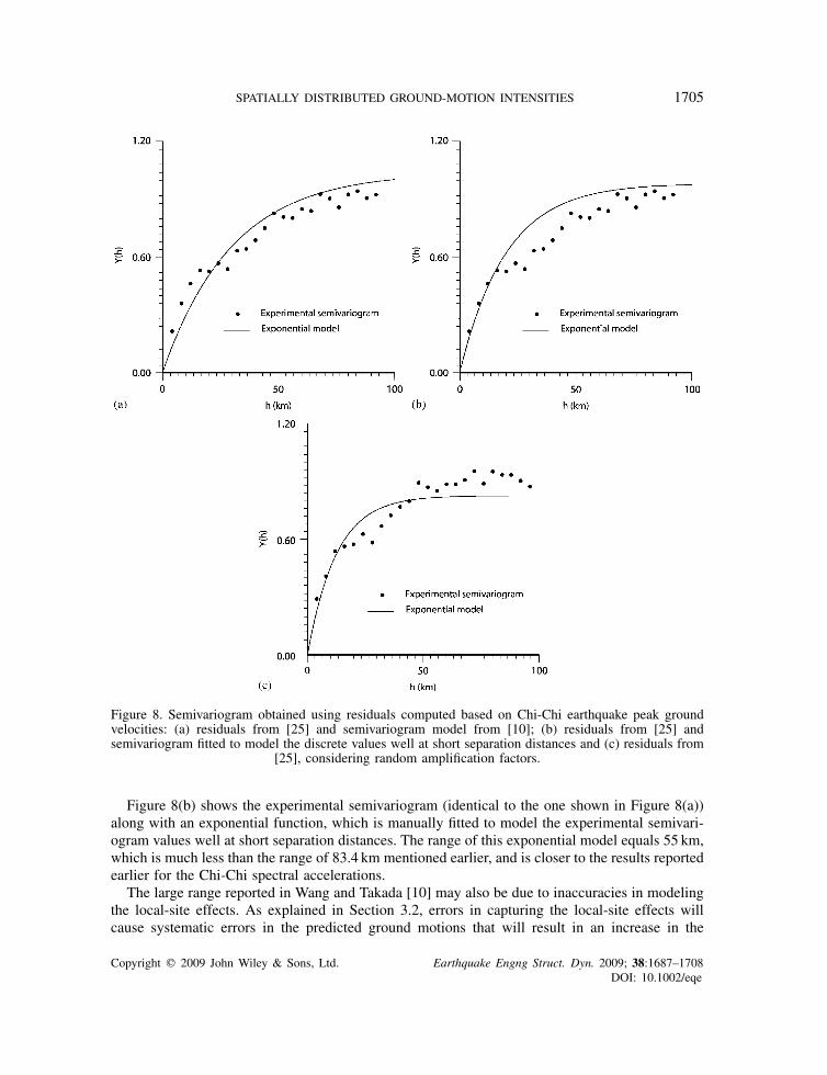
Figure 8. Semivariogram obtained using residuals computed based on Chi-Chi earthquake peak groundvelocities: (a) residuals from [25] and semivariogram model from [10]; (b) residuals from [25] andsemivariogram fitted to model the discrete values well at short separation distances and (c) residuals from

[25], considering random amplification factors.

Figure 8(b) shows the experimental semivariogram (identical to the one shown in Figure 8(a))along with an exponential function, which is manually fitted to model the experimental semivari-ogram values well at short separation distances. The range of this exponential model equals 55 km,which is much less than the range of 83.4 km mentioned earlier, and is closer to the results reportedearlier for the Chi-Chi spectral accelerations.

The large range reported in Wang and Takada [10] may also be due to inaccuracies in modelingthe local-site effects. As explained in Section 3.2, errors in capturing the local-site effects willcause systematic errors in the predicted ground motions that will result in an increase in the



range of the semivariogram. Using a constant amplification factor of 2.0 (without consideringthe actual local-site effects) will produce even larger systematic errors in the predicted groundmotions than considered previously. Consider a complementary hypothetical example in whichthe ground-motion amplification factor for each site is considered to be an independent randomvariable, uniformly distributed between 1.0 and 2.0. Randomizing the ground-motion amplificationwill break up the correlation between the prediction errors in a cluster of closely spaced sites. Thesemivariogram of residuals obtained by considering such random amplification factors is shownin Figure 8(c). The range of this semivariogram equals 43 km, which is less than the 55 km fromFigure 8(b). The true amplifications are neither constant at 2.0, nor are totally random between 1.0and 2.0. Hence, the range of the semivariogram is expected to lie within 43 km and 55 km, whichis close to the range observed using short period spectral accelerations in the current work.

Boore et al. [11] estimated correlations between residuals computed from the Northridge earth-quake PGAs. They observed that the correlations dropped to zero when the inter-site separationdistance was approximately 10 km. This matches with the range of 10 km estimated in the currentwork using the Northridge earthquake PGAs (Figure 2(a)). Those results appear to be consistentwith the results shown here (and it is interesting to note that the two efforts used different estimationprocedures and data sets).

The observations in the current work are also consistent with those reported in Goda and Hong[9] who reported a more rapid decrease in correlations with distance for the Northridge earthquakeground motions than for the Chi-Chi earthquake ground motions. They also reported that the decayof spatial correlation of the residuals computed from spectral accelerations is more gradual atlonger periods, a feature observed and analyzed in the current research work. The current workadds plausible physical explanations for these empirically observed trends.

6. CONCLUSIONS

Geostatistical tools have been used to quantify the correlation between spatially distributed ground-motion intensities. The correlation is known to decrease with increase in the separation betweenthe sites, and this correlation structure can be modeled using semivariograms. A semivariogramis a measure of the average dissimilarity between the data, whose functional form, sill and rangeuniquely identify the ground-motion correlation as a function of separation distance.

Ground motions observed during the Northridge, Chi-Chi, Big Bear City, Parkfield, AlumRock, Anza and Chino Hills earthquakes were used to compute the correlations between spatiallydistributed spectral accelerations, at various spectral periods. The correlations were computed fornormalized intra-event residuals, since the normalized intra-event residuals will be homoscedastic.The ground-motion model of Boore and Atkinson [1] was used for the computations, but theresults did not change when the Chiou and Youngs [3] model was used instead.

It was seen that the rate of decay of the correlation with separation typically decreases withincreasing spectral period. It was reasoned that this could be because long period ground motionsat two different sites tend to be more coherent than short period ground motions, on account oflesser wave scattering during propagation. It was also observed that, at periods longer than 2 s, theestimated correlations were similar for all the earthquake ground motions considered. At shorterperiods, however, the correlations were found to be related to the site Vs30 values. It was shownthat the clustering of site Vs30’s is likely to result in larger correlations between residuals. Based onthese findings, a predictive model was developed that can be used to select appropriate correlation



estimates for use in risk assessment of spatially distributed building portfolios or infrastructuresystems.

The research work also investigates the effect of directivity on the correlations using pulse-like ground motions. The correlations obtained were similar to those estimated using all groundmotions. The results, however, are not discussed in detail due to concerns about the reliability of theresults on account of the small data set of pulse-like ground motions. The work also investigatedthe commonly used assumption of isotropy in the correlation between residuals using directionalsemivariograms. If directional semivariograms computed based on different azimuths are identicalto the omni-directional semivariogram (which is obtained assuming isotropy), it can be concludedthat the semivariograms (and therefore, the correlations) are isotropic. It was seen using empiricaldata that the correlation between Chi-Chi and Northridge earthquake intensities show isotropy atboth short and long periods.

The results obtained were also compared with those reported in the literature [9–11]. Wangand Takada [10] report larger correlations using the PGVs computed using the Chi-Chi earthquakerecordings than those reported in this work for spectral accelerations. It was shown that these largercorrelations are a result of attempting to fit the experimental semivariogram reasonably well overthe entire range of separation distances of interest (which is a typical result of using least-squaresfits and eye-ball fits that produce results similar to least-squares fits), and of using a ground-motionmodel that does not account for the effect of local-site conditions. Typically, a semivariogrammodel should represent correlations accurately at small separations since ground motions at a siteare more influenced by ground motions at nearby sites. The method of least squares assigns equalimportance to all separation distances and is therefore, inefficient. In the current research work,semivariogram models are fitted manually with emphasis on accurately modeling correlations atsmall separations.

This study illustrates various factors that affect the spatial correlation between ground-motionintensities, and provides a basis to choose an appropriate model using empirical data. The proposedpredictive model can be used for obtaining the joint distribution of spatially distributed ground-motion intensities, which is necessary for a variety of seismic hazard calculations.

ACKNOWLEDGEMENTS

The authors thank the two anonymous reviewers for their helpful reviews of the manuscript. The authorsalso thank Paolo Bazzurro and Jaesung Park from AIR Worldwide Co. for useful discussions on thisresearch topic. This work was supported by the U.S. Geological Survey (USGS) via External ResearchProgram award 07HQGR0031. Any opinions, findings and conclusions or recommendations expressed inthis material are those of the authors and do not necessarily reflect those of the USGS.

REFERENCES

1. Boore DM, Atkinson GM. Ground-motion prediction equations for the average horizontal component of PGA,PGV and 5% damped SA at spectral periods between 0.1 s and 10.0 s. Earthquake Spectra 2008; 24(1):99–138.

2. Abrahamson NA, Silva WJ. Summary of the Abrahamson & Silva NGA ground-motion relations. EarthquakeSpectra 2008; 24(1):99–138.

3. Chiou BS-J, Youngs RR. An NGA model for the average horizontal component of peak ground motion andresponse spectra. Earthquake Spectra 2008; 24(1):173–215.

4. Campbell KW, Bozorgnia Y. NGA ground motion model for the geometric mean horizontal component of PGA,PGV, PGD and 5% damped linear elastic response spectra for periods ranging from 0.1 to 10 s. EarthquakeSpectra 2008; 24(1):139–171.



5. Lee R, Kiremidjian AS. Uncertainty and correlation for loss assessment of spatially distributed systems. EarthquakeSpectra 2007; 23(4):743–770.

6. Bazzurro P, Luco N. Effects of different sources of uncertainty and correlation on earthquake-generated losses.Presented at IFED: International Forum on Engineering Decision Making, Stoos, Switzerland, 2004.

7. Park J, Bazzurro P, Baker JW. Modeling spatial correlation of ground motion intensity measures for regionalseismic hazard and portfolio loss estimation. Tenth International Conference on Application of Statistic andProbability in Civil Engineering (ICASP10), Tokyo, Japan, 2007.

8. Jayaram N, Baker JW. Statistical tests of the joint distribution of spectral acceleration values. Bulletin of theSeismological Society of America 2008; 98(5):2231–2243.

9. Goda K, Hong HP. Spatial correlation of peak ground motions and response spectra. Bulletin of the SeismologicalSociety of America 2008; 98(1):354–365.

10. Wang M, Takada T. Macrospatial correlation model of seismic ground motions. Earthquake Spectra 2005;21(4):1137–1156.

11. Boore DM, Gibbs JF, Joyner WB, Tinsley JC, Ponti DJ. Estimated ground motion from the 1994 Northridge,California, earthquake at the site of the Interstate 10 and La Cienega Boulevard bridge collapse, West LosAngeles, California. Bulletin of the Seismological Society of America 2003; 93(6):2737–2751.

12. Deutsch CV, Journel AG. Geostatistical Software Library and User’s Guide. Oxford University Press: Oxford,New York, 1998.

13. Goovaerts P. Geostatistics for Natural Resources Evaluation. Oxford University Press: Oxford, New York, 1997.14. Chiou B, Darragh R, Gregor N, Silva W. NGA project strong-motion database. Earthquake Spectra 2008;

24(1):23–44.15. Baker JW, Jayaram N. Effects of spatial correlation of ground-motion parameters for multi-site risk assessment:

collaborative research with Stanford University and AIR. Technical Report, Report for U.S. Geological SurveyNational Earthquake Hazards Reduction Program (NEHRP) External Research Program Awards 07HQGR0031,2009. Available from: http://earthquake.usgs.gov/research/external/reports/07HQGR0031.pdf.

16. Bazzurro P, Park J, Tothong P, Jayaram N. Effects of spatial correlation of ground-motion parameters for multi-siterisk assessment: collaborative research with Stanford University and AIR. Technical Report, Report for U.S.Geological Survey National Earthquake Hazards Reduction Program (NEHRP) External Research Program Awards07HQGR0032, 2009. Available from: http://earthquake.usgs.gov/research/external/reports/07HQGR0032.pdf.

17. Der Kiureghian A. A coherency model for spatially varying ground motions. Earthquake Engineering andStructural Dynamics 1996; 25:99–111.

18. Zerva A, Zervas V. Spatial variation of seismic ground motions. Applied Mechanics Reviews 2002; 55(3):271–297.19. Castellaro S, Mulargia F, Rossi PL. Vs30: proxy for seismic amplification. Seismological Research Letters 2008;

79(4):540–543.20. Borcherdt RD. Estimates of site-dependent response spectra for design (methodology and justification). Earthquake

Spectra 1994; 10:617–653.21. Baker JW. Quantitative classification of near-fault ground motions using wavelet analysis. Bulletin of the

Seismological Society of America 2007; 97(5):1486–1501.22. CESMD database. Available from: http://www.strongmotioncenter.org (last accessed 6 June 2008), 2008.23. Global Vs30 map server. Available from: http://earthquake.usgs.gov/research/hazmaps/interactive/vs30/ (last

accessed 21 September 2008), 2008.24. KiK Net. Available from: http://www.kik.bosai.go.jp/ (last accessed 12 December 2007), 2007.25. Annaka T, Yamazaki F, Katahira F. Proposal of peak ground velocity and response spectra based on JMA 87

type accelerometer records. Proceedings, 27th JSCE Earthquake Engineering Symposium, Tokyo, Japan, vol. 1,1997; 161–164.

26. Hayashi T, Fukushima S, Yashiro H. Effects of the spatial correlation in ground motion on the seismic riskof portfolio of buildings. First European Conference on Earthquake Engineering and Seismology, Geneva,Switzerland, 2006.

27. Kutner MH, Nachtsheim CJ, Neter J, Li W. Applied Linear Statistical Models. The McGraw-Hill CompaniesInc.: New York, 2005.


Correlation model for spatially distributed ground …bakerjw/Publications/Jayaram_Baker_(2009...The estimated correlation model is also compared with previously published results,

Documents