CORRELATION BETWEEN GEOTECHNICAL AND GEOPHYSICAL PROPERTIES OF SOIL by NASTARAN SHIRGIRI A Thesis submitted to The University of Birmingham For the degree of MASTER OF PHILOSOPHY School of CIVIL ENGINEERING College of ENGINEERING AND PHYSICAL SCIENCES The University of Birmingham April 2012

Welcome message from author
This document is posted to help you gain knowledge. Please leave a comment to let me know what you think about it! Share it to your friends and learn new things together.
Transcript
CORRELATION BETWEEN GEOTECHNICAL AND
GEOPHYSICAL PROPERTIES OF SOIL
by
NASTARAN SHIRGIRI
A Thesis submitted to The University of Birmingham
For the degree of MASTER OF PHILOSOPHY
School of CIVIL ENGINEERING College of ENGINEERING AND PHYSICAL SCIENCES The University of Birmingham April 2012

University of Birmingham Research Archive
e-theses repository This unpublished thesis/dissertation is copyright of the author and/or third parties. The intellectual property rights of the author or third parties in respect of this work are as defined by The Copyright Designs and Patents Act 1988 or as modified by any successor legislation. Any use made of information contained in this thesis/dissertation must be in accordance with that legislation and must be properly acknowledged. Further distribution or reproduction in any format is prohibited without the permission of the copyright holder.
i
ABSTRACT
In the UK road network, it is estimated that up to 4 million holes are cut each year in order to
install or repair buried service pipes and cables, and it is important to identify the location of
existing buried assets prior to such works if the numerous potential practical problems such
as unforeseen costs and dangers for utility owners, contractors and road users are to be
avoided. The Mapping the Underworld research team is attempting to develop the means to
locate, map in 3-D and record the position of all buried utility assets without excavation. To
realise this aim four different kinds of technologies are being studied: ground penetrating
radar, acoustics, low frequency active electromagnetic fields and passive electromagnetic
fields. All these techniques need waves to travel through the ground and they are affected by
the ground properties.
Geophysical techniques, such as the seismic surface wave technique, offer a non-intrusive
and non-destructive way of analysing the ground and potentially providing measurements of
geotechnical properties. However, we need to be careful in comprehending the relationships
between geophysical techniques and geotechnical ground properties to ensure reliable
interpretation and so as not to overrate the results that geophysics can accomplish.
This research discusses the model testing for Kaolin and OxfordClay, which was carried out
to help to understand seismic surface wave results in relation to the geotechnical properties of
the soils. The surface wave tests were initially carried out to establish an optimal
methodology for the evaluation of this correlation as well as to prove the accuracy of the
equipment and its system for surface wave testing at the laboratory scale. The surface wave

ii
technique generated and recorded the shear waves in the soil samples, enabling a shear
modulus profile to be determined for the two soils over a range of water contents from
significantly wet to significantly dry of the optimum water content (and hence maximum dry
density) of the compacted clay soils. This made it possible to vary the subsurface velocity
with different variations in water content and density over short distances.
The relationships obtained from the controlled tests showed close agreement to those reported
in literature, but that the literature only considers a narrow range of water contents. The test
results demonstrated that the shear wave velocity, and hence the shear modulus, decrease
with increasing moisture content. Importantly the test results also indicated that the shear
wave velocity, hence shear modulus, has an inverse relation with density before it reaches the
optimum water content (or maximum dry density) after which they exhibit a direct
relationship, i.e. the shear wave velocity decreases while the density decreases.

iii
DEDICATION
To my parents, of course; Kian & Mahmood
There is no doubt in my mind that without their Continued support and counsel
I could not have completed this process

iv
ACKNOWLEDGMENTS This thesis was made possible by the support and assistance of a number of people whom would like to personally thank. I am heartily thankful to my supervisor Prof. Chris Rogers for giving me the opportunity to carry out this Thesis and for being a great supervisor. Thank you for all your patience, help, support and guidance throughout the process. I would also like to thank Dr. Nicole Metje as my co-supervisors., for all the advice and encouragement. I would like to acknowledge gratefully for the assistance receive from the following: Dr G.Ghataora and Dr I. Jefferson for their opinion and advice. Mr. Aziman Madun for all his time, help and advice. Mr Phillip Robert Atkins for lending his laboratory testing equipment, as well as sharing his knowledge and experience on the testing and the signal processing. Dr David Gunn for his helps in my early understanding of seismic surface wave. Lab technicians’ Mr Michael Vanderstam, Mr David Cope, Mr Jim White, Mr Nathan and Mr Bruce Reed for their support. Miss Lyn Hipwood for her helps, time and support. Mr Mark Britton, for all his helps. Friends and post graduate members’ in room F59B (November 2009 to April 2012) for their help and support. Finally members of my family and my lovely friends, specially Saba Ghasemi, for their help and support.
v
Table of Contents
ABSTRACT…………………………………………………………………………….. i
DEDICATION………………………………………………………………………….. iii
ACKNOWLEDGMENTS………………...………………………………...................... iv
LIST OF FIGURES……………………………………………………………………... viii
LIST OF TABLES…………………………………..……………………....................... xii
LIST OF ABBREVIATIONS………………………….................................................... xiv
Chapter 1 …………………………………………………........................................... 1
1.1 Introduction………………………………………....................................... 1
1.2 Research Aim and Objectives……………………....................................... 3
1.3 Outline of thesis……………………………………………………............ 4
Chapter 2 ……………………………………………………………........................... 6
2.1 Introduction………………………………………….…………………….. 6
2.2 Overview of Geophysical Techniques…………………….………………. 7
2.2.1 Ground Penetration Radar (GPR) …………….…………………. 9
2.2.2 Electrical Resistivity ……………………………………………… 11
2.2.3 Seismic –based Methods …………………….…………………… 12
2.3 Seismic Waves …………………………………………………………... 14
2.3.1 Body Waves ……………………….…………………………….. 16
2.3.2 Surface Waves ………………….....……………………………… 20
2.3.2.1 Spectral Analysis of Surface Waves (SASW) …..………… 22
2.3.2.2 Continuous Surface Wave (CSW) …….…………………… 24
2.3.2.3 Multi-Channel Surface Waves (MASW) ….……………….. 27
2.4 Surface Wave Method …………………………………….……………. 29
2.5 Relationship of Seismic to Geotechnical Parameters …..………………. 31
2.6 Experimental Relationships and Data From The Literature …............... 34
2.7 Summary ………………………………………………………………. 44

vi
Chapter 3 …………………………………………………………………………….. 45
3.1 Introduction ……………………………………………………………. 45
3.2 Establishing Laboratory Seismic Surface Wave Equipment …………. 47
3.2.1 Seismic Surface Wave Equipment …………................................ 49
3.3 Experimental Procedure ……………………………………………….. 53
3.4 Method for Data Processing …………………………..………………. 54
Chapter 4 ………………………………………….…………………………………. 59
4.1 Introduction …………………………………………………………... 59
4.2 Data Processing …………………………...……................................... 59
Chapter 5 ……………………………………….……………………………………. 64
5.1 Introduction ………………………………………................................ 64
5.2 Clay Materials Used in Test Beds …………………............................... 64
5.2.1 Plasticity Measurements ……………………………………….. 65
5.2.2 Specific Gravity ……………….................................................... 66
5.2.3 Compaction Test ………………………………………………… 66
5.3 Preparation of Kaolin clay Test Bed ………………………………….. 67
5.4 Preparation of Oxford clay Test Bed ………………………………….. 69
5.5 Preparation of The Test Bed ………….………………………………… 71
5.6 Seismic Test ………………………….................................................... 72
Chapter 6 ……………………………………….……………………………………. 76
6.1 Introduction ……………………………………..................................... 76
6.2 Kaolin clay- 28% Moisture Content …………………………………... 76
6.2.1 Repeatability of the tests- Kaolin clay ………............................... 82
6.2.2 Kaolin clay, 24% and 33% Moisture Content …………………... 86
6.3 Homogeneous Oxford clay- 32% Moisture Content …………............... 93
6.3.1 Repeatability of the tests- Oxford clay …………………………. 97
6.3.2 Oxford clay, 19% and 24% Moisture Content ............................... 101
6.4 Discussion …………………….……….................................................. 107

vii
Chapter 7 …………………………………………………………………………….. 109
7.1 Introduction ……………………………................................................. 109
7.2 Equipment and System ……………………………………………….. 109
7.3 Clay Model …………………………………………………………….. 110
7.3.1 Phase and Shear Wave Velocity Variations ……………………… 110
7.3.1.1 Kaolin Clay …………………............................................. 110
7.3.1.2 Oxford Clay ………………………...…………………….. 115
7.3.2 Shear Modulus …………………………………………………… 119
7.3.3 Shear Wave Velocity, Density and Moisture Content ................. 123
Chapter 8 …………………………………………………………………………….. 127
8.1 Introduction …………………………………………………………… 127
8.2 Main Outcomes …………….………………………………………….. 128
8.3 Recommendations for Future Studies ………………………………….. 130
REFERENCES ………………………………………………………………………. 132
viii
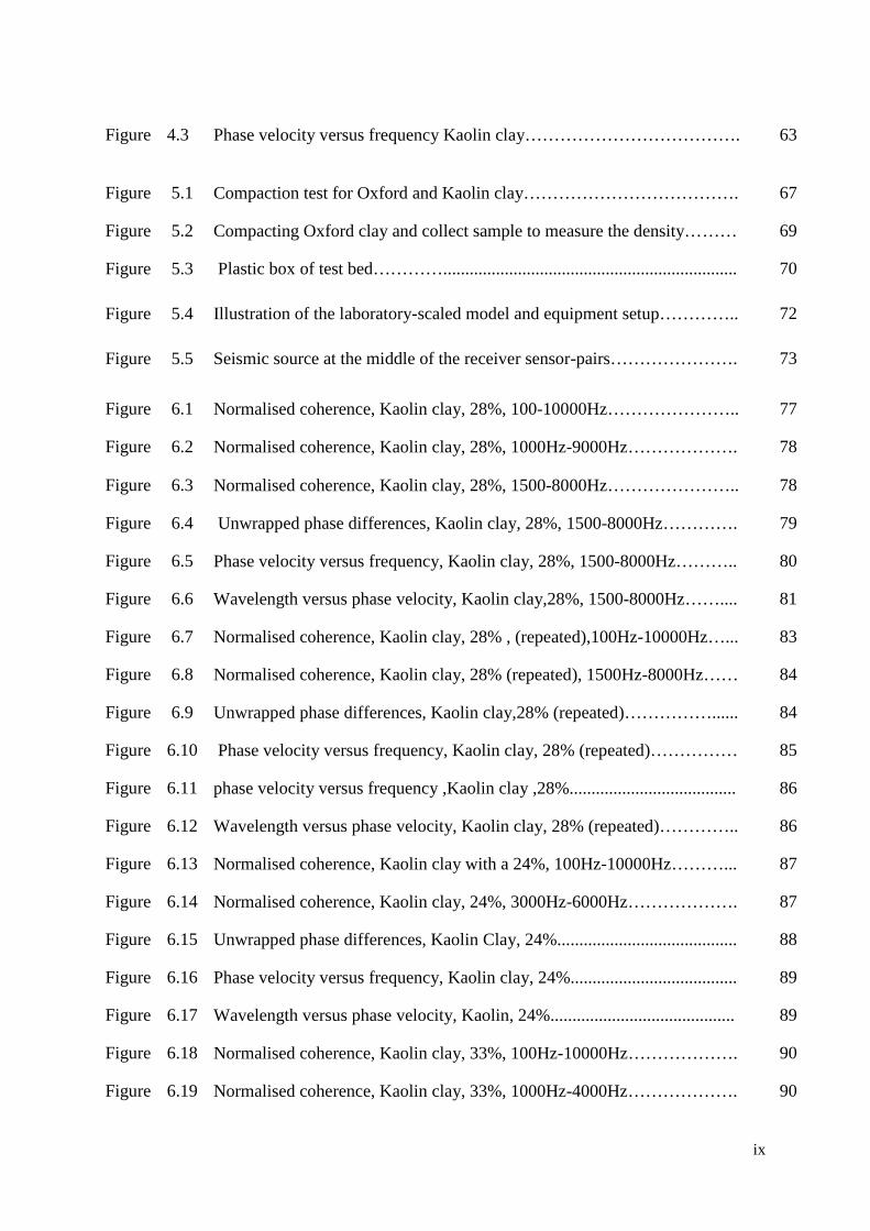
LIST OF FIGURES
Figure 2.1 GPR, electrical resistivity equipment seismic based method……………… 8
Figure 2.2 V, I and R, the parameters of Ohm’s law…………………………………... 11
Figure 2.3 Resistivity…………………………………………………………………... 12
Figure 2.4 the Schematic elastic wave propagation in ground………………………… 15
Figure 2.5 (a) Reflection and (b) Refraction…………………………………………… 17
Figure 2.6 Rayleigh wave dispersion………………………………………………….. 22
Figure 2.7 In an SASW measurement…………………………………………………. 24
Figure 2.8 Schematic diagram showing the steps for CSW technique……................... 27
Figure 2.9 MASW field data collection………………………………………………... 29
Figure 2.10 Modulus Variations with Strain Level…...................................................... 32
Figure 2.11 Bender Element Wave Generation…………………………………………. 33
Figure 2.12 Characteristic ranges of soil stiffness modulus…………………………….. 34
Figure 2.13 Variation of shear wave velocity with depth………..................................... 36
Figure 2.14 Distribution of shear velocity and water content with depth………………. 39
Figure 2.15 Shear modulus versus wave length- Oxford Clay 32%................................. 42
Figure 2.16 Shear modulus versus wave length- Oxford Clay 40%................................. 42
Figure 2.17 Variation of S-wave velocity with degree of saturation …………………… 43
Figure 3.1 The seismic surface wave factors…….......................................................... 48
Figure 3.2 Outline details of the Initial and Main laboratory scale model tests……….. 49
Figure 3.3 Electromechanical vibrator -absorber pad…………………………………. 50
Figure 3.4 Piezo-ceramic transducer located on sample……………………………….. 50
Figure 3.5 Detail of the equipment…………………………………………………….. 51
Figure 3.6 Laboratory setup for seismic surface wave test…………………………..... 52
Figure 3.7 photograph of the equipment……………………………………………….. 52
Figure 3.8 Illustration of the laboratory-scale model and equipment setup………........ 53
Figure 3.9 data collection process…………………………………………………....... 54
Figure 4.1 The phase differences for the 2 sensor-pairs Kaolin Clay …………………. 61
Figure 4.2 The Normalised coherence between channels A and B Kaolin Clay…........ 62
ix
Figure 4.3 Phase velocity versus frequency Kaolin clay………………………………. 63
Figure 5.1 Compaction test for Oxford and Kaolin clay………………………………. 67
Figure 5.2 Compacting Oxford clay and collect sample to measure the density……… 69
Figure 5.3 Plastic box of test bed…………................................................................... 70
Figure 5.4 Illustration of the laboratory-scaled model and equipment setup………….. 72
Figure 5.5 Seismic source at the middle of the receiver sensor-pairs…………………. 73
Figure 6.1 Normalised coherence, Kaolin clay, 28%, 100-10000Hz………………….. 77
Figure 6.2 Normalised coherence, Kaolin clay, 28%, 1000Hz-9000Hz………………. 78
Figure 6.3 Normalised coherence, Kaolin clay, 28%, 1500-8000Hz………………….. 78
Figure 6.4 Unwrapped phase differences, Kaolin clay, 28%, 1500-8000Hz…………. 79
Figure 6.5 Phase velocity versus frequency, Kaolin clay, 28%, 1500-8000Hz……….. 80
Figure 6.6 Wavelength versus phase velocity, Kaolin clay,28%, 1500-8000Hz…….... 81
Figure 6.7 Normalised coherence, Kaolin clay, 28% , (repeated),100Hz-10000Hz…... 83
Figure 6.8 Normalised coherence, Kaolin clay, 28% (repeated), 1500Hz-8000Hz…… 84
Figure 6.9 Unwrapped phase differences, Kaolin clay,28% (repeated)……………...... 84
Figure 6.10 Phase velocity versus frequency, Kaolin clay, 28% (repeated)…………… 85
Figure 6.11 phase velocity versus frequency ,Kaolin clay ,28%...................................... 86
Figure 6.12 Wavelength versus phase velocity, Kaolin clay, 28% (repeated)………….. 86
Figure 6.13 Normalised coherence, Kaolin clay with a 24%, 100Hz-10000Hz………... 87
Figure 6.14 Normalised coherence, Kaolin clay, 24%, 3000Hz-6000Hz………………. 87
Figure 6.15 Unwrapped phase differences, Kaolin Clay, 24%......................................... 88
Figure 6.16 Phase velocity versus frequency, Kaolin clay, 24%...................................... 89
Figure 6.17 Wavelength versus phase velocity, Kaolin, 24%.......................................... 89
Figure 6.18 Normalised coherence, Kaolin clay, 33%, 100Hz-10000Hz………………. 90
Figure 6.19 Normalised coherence, Kaolin clay, 33%, 1000Hz-4000Hz………………. 90

x
Figure 6.20 unwrapped phase differences , Kaolin clay ,33%.......................................... 91
Figure 6.21 Phase velocity versus frequency, Kaolin clay, 33%...................................... 92
Figure 6.22 Wavelength versus phase velocity, Kaolin clay, 33%................................... 92
Figure 6.23 Typical coherence, Oxford clay, 32% 100Hz-10000Hz……………........... 94
Figure 6.24 Normalised coherence, Oxford clay, 32% 1000Hz-5000Hz…………......... 94
Figure 6.25 Unwrapped phase differences s, Oxford clay, 32%...................................... 95
Figure 6.26 Phase velocity versus frequency, Oxford clay, 32%..................................... 96
Figure 6.27 Wavelength versus phase velocity, Oxford clay, 32% ……………….......... 97
Figure 6.28 Normalised coherence, Oxford clay, 32 %( repeated), 100Hz-10000Hz...... 98
Figure 6.29 Normalised coherence, Oxford clay, 32 %( repeated), 1000Hz-5000Hz….. 99
Figure 6.30 Unwrapped phase differences, Oxford clay, 32%......................................... 99
Figure 6.31 phase velocity versus frequency, Oxford clay ,32%..................................... 100
Figure 6.32 phase velocity versus frequency ,Oxford clay , 32%.................................... 100
Figure 6.33 Wavelength versus phase velocity, Oxford clay, 32% (repeated)…............ 101
Figure 6.34 Normalised coherence, Oxford clay, 24%.................................................... 102
Figure 6.35 Normalised coherence, Oxford clay, 24%.................................................... 102
Figure 6.36 Unwrapped phase differences, Oxford Clay, 24%........................................ 103
Figure 6.37 Phase velocity versus frequency, Oxford clay, 24%.................................... 104
Figure 6.38 Wavelength versus phase velocity, Oxford clay, 24%.................................. 104
Figure 6.39 Normalised coherence, Oxford clay, 19% moisture content…………......... 105
Figure 6.40 Normalised coherence, Oxford clay, 19%.................................................... 105
Figure 6.41 unwrapped phase differences ,Oxford clay ,19%.......................................... 106
Figure 6.42 Phase velocity versus frequency, Oxford clay, 19%..................................... 107
Figure 6.43 Wavelength versus phase velocity, Oxford clay, 19%.................................. 107
Figure 7.1 Phase velocity versus frequency, 1500-8000 Hz, Kaolin clay……………... 112

xi
Figure 7.2 Phase velocity variation, 3000-4000 Hz, Kaolin clay……………………… 112
Figure 7.3 Shear wave velocity versus frequency, 1500-8000 Hz, Kaolin clay……..... 114
Figure 7.4 Shear wave velocity variation, 3000-4000 Hz, Kaolin clay……………...... 114
Figure 7.5 phase velocity versus frequency,1000-7000 Hz, Oxford clay…………....... 115
Figure 7.6 phase velocity variation , of 2000-5000 Hz, Oxford clay…………….......... 116
Figure 7.7 shear wave velocity versus frequency,1000-7000 Hz, Oxford Clay……….. 117
Figure 7.8 shear wave velocity,2000-5000 Hz, Oxford Clay…………………………. 118
Figure 7.9 shear wave velocity, shear modulus, Kaolin clay………………………….. 120
Figure 7.10 shear wave velocity ,shear modulus , Oxford clay…………………………. 121
Figure 7.11 Variation of shear modulus, Kaolin Clay………………………………....... 121
Figure 7.12 Variation of shear modulus, Oxford clay………………………………....... 122
Figure 7.13 Shear Modulus profile at different depth, Kaolin clay……………………... 123
Figure 7.14 Shear Modulus profile at different depth, Oxford clay…………………….. 123
Figure 7.15 Shear wave velocity, moisture content and density, Kaolin clay…………... 125
Figure 7.16 Shear wave velocity, moisture content and density, Oxford clay…….......... 125
xii
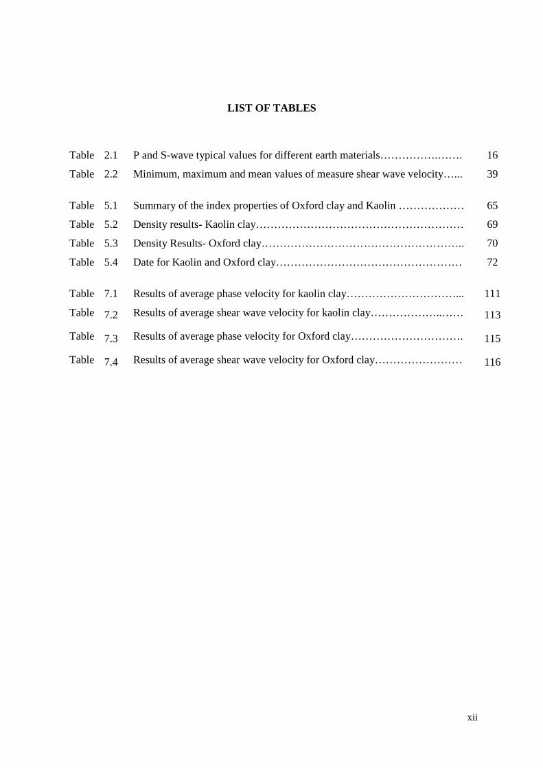
LIST OF TABLES
Table 2.1 P and S-wave typical values for different earth materials…………….……. 16
Table 2.2 Minimum, maximum and mean values of measure shear wave velocity…... 39
Table 5.1 Summary of the index properties of Oxford clay and Kaolin ……………… 65
Table 5.2 Density results- Kaolin clay………………………………………………… 69
Table 5.3 Density Results- Oxford clay……………………………………………….. 70
Table 5.4 Date for Kaolin and Oxford clay…………………………………………… 72
Table 7.1 Results of average phase velocity for kaolin clay…………………………... 111
Table 7.2 Results of average shear wave velocity for kaolin clay………………..…… 113
Table 7.3 Results of average phase velocity for Oxford clay…………………………. 115
Table 7.4 Results of average shear wave velocity for Oxford clay…………………… 116
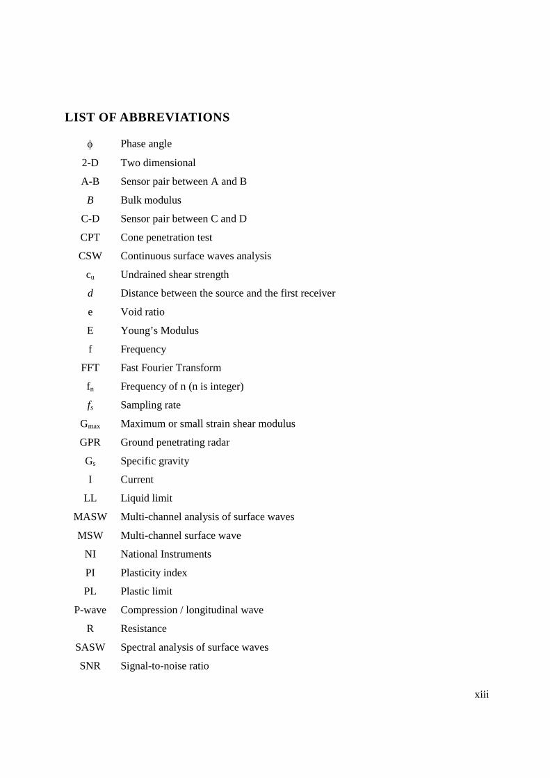
LIST OF ABBREVIATIONS
Phase angle
2-D Two dimensional
A-B Sensor pair between A and B
B Bulk modulus
C-D Sensor pair between C and D
CPT Cone penetration test
CSW Continuous surface waves analysis
cu Undrained shear strength
d Distance between the source and the first receiver
e Void ratio
E Young’s Modulus
f Frequency
FFT Fast Fourier Transform
fn Frequency of n (n is integer)
fs Sampling rate
Gmax Maximum or small strain shear modulus
GPR Ground penetrating radar
Gs Specific gravity
I Current
LL Liquid limit
MASW Multi-channel analysis of surface waves
MSW Multi-channel surface wave
NI National Instruments
PI Plasticity index
PL Plastic limit
P-wave Compression / longitudinal wave
R Resistance
SASW Spectral analysis of surface waves
SNR Signal-to-noise ratio
xiii

S-wave Shear / transverse wave
V Voltage
w Water content
Δx Spacing between the receivers
λ Wave length
ω Angular frequency (ω = 2πf)
Poisson’s ratio
p Compression / longitudinal wave velocity
s Shear wave velocity
r Rayleigh wave / phase velocity
kyn Time-domain signal at n discrete sample and time k
fYn Spectrum of the signal at n discrete sample and frequency f
)(wmn Phase difference between receivers m and n at frequency w.
Soil bulk density
w Water density
xiv
1
Chapter 1
INTRODUCTION
1.1 Introduction
In the UK road network, it is estimated that up to 4 million holes are cut each year in order to
identify the location of existing buried assets when installing or repairing buried service pipes
and cables. This results in numerous practical problems such as indirect and other costs and
danger for utility owners, contractors and road users (Mapping the Underworld [online]).
Therefore, the Mapping the Underworld research group is trying to develop the means to
locate, map in 3-D and record the position of all buried utility assets without excavation. To
reach this aim three different kinds of technologies are being studied: ground penetrating
radar, acoustics, and low frequency active and passive electromagnetic fields. All these
techniques need waves to travel through the ground and these waves are affected by the
ground properties.
Geophysical techniques such as ground penetrating radar, electrical resistivity, and magnetism
are convenient and use specific imaging equipment. However to use these methods entails
skill, good knowledge and information on the geological model of the area, and support from
2
borehole data to interpret the results (Crice, 2005). Considering an example, there are
shortfalls of using ground penetrating radar in obtaining deeper results when dealing with high
conductivity material such as marine clays or saturated clays. The resistivity of soils differs
depending on the moisture content and the soil type. The degree of soil resistance is chiefly
controlled by the movement of charged ions in pore fluids. As a result, the salinity, porosity
and fluid saturation tend to govern electrical resistivity measurements (Giao et al., 2003).
Conversely, seismic wave techniques that are reliant on the modulus and density of the
materials can be used to determine very useful parameters for engineering purposes, such as
elastic modulus, shear modulus and Poisson’s ratio, and are most effective when soils are
saturated (as is often the case in the UK).
As such, geophysical techniques, like the seismic surface wave technique, offer a non-
intrusive and non-destructive way of performing geotechnical properties measurements.
Moreover, geophysical approaches such as this provide a cost effective way to investigate
conditions on a test site. At the same time these methods help to overcome major shortfalls of
classical analytical approaches. It is evident that geophysical testing can create very
considerable high quality results. However, there is a need to be careful in comprehending the
geophysical techniques, and essentially the disadvantages, so as not to overrate the results that
geophysics can accomplish (Clayton et al., 1995).
The transmission of the seismic waves is in the form of body waves and surface waves.
However the difference is that body waves are usually non-dispersive. In a solid and
homogeneous medium, the velocity of surface waves does not oscillate drastically as a
function of the distance propagated. However, when the properties of the medium vary with
depth, surface waves become dispersive in a manner that the velocity of the propagation
varies with respect to wavelength and frequency. Surface waves are also relatively less
3
attenuated as a function of the transmission distance when compared to body waves. These
two characteristics make it practical to apply surface wave analysis for the survey of near-
surface soil properties, and thus in turn the survey of any changes to these properties that
subsequently occur.
Classical surface wave techniques that use a single pair of receivers generally yield one-
dimensional results of phase velocity versus depth. In a laterally heterogeneous medium,
however, it is more appropriate to use multi-channel receivers so as to avoid discrepancies. It
is important to present a plot of the phase velocity against depth as a function of the lateral
distance. Tallavo et al. (2009) have applied this method for the detection of buried timber
trestles.
Therefore, the surface wave technique is used in the research reported herein to generate the
phase velocities, which then were transformed to shear waves. With this, a shear modulus
profile was then created and examined. The data processing technique was vital since it made
it possible to vary the subsurface velocity with different variations in density over short
distances. The results were further studied while considering the model properties and the
configuration. Hence this research has been carried out to help to understand seismic surface
wave result in relation to the geotechnical properties of the soils which is a related to the aim
of the Mapping the Underworld group for design and construction of a prototype acoustic
sensor to determine the acoustic technologies for locating the buried utility service location.
1.2 Research Aim and Objectives
The aim of the study is to assess how soil properties influence acoustic wave transmission and
how they can be used to develop a correlation between acoustic and geotechnical properties.
To achieve this aim, the following objectives were established:

4
• Conduct an extensive literature review to critically assess the current knowledge and
determine where there are gaps in knowledge with respect to seismic wave
propagation through the ground
• Identify suitable seismic surface wave equipment for laboratory scale tests
• Develop a laboratory test to identify the influence of geotechnical soil properties on
the propagation of the seismic waves and geophysical properties of soil
• Determine a suitable range of soils and soil conditions for the laboratory experiments
in order to determine the correlation between geophysical and geotechnical properties
of soils
1.3 Outline of Thesis
Chapter 2 presents a brief introduction to the use of geophysics, which includes an overview
on various geophysical methods, types of seismic wave and a general description of the
relationship between Seismic and Geotechnical Parameters. Chapter 3 describes the initial
testing method for laboratory testing, which involved the development of equipment and its
operational system. Sample preparation, development of the test equipment and measurement
procedures are established for the seismic surface wave experimental work. Chapter 4 shows
the possibility of the test procedure and a brief introduction to data processing and result
analysis. Chapter 5 presents the geotechnical properties of clay materials used in the tests, the
preparation of the test bed, the seismic surface wave testing arrangement and the data
processing techniques. In Chapter 6 the test results are analysed, compared and discussed in
detail. In Chapter 7, results are discussed and correlations are made between the seismic wave
results and geotechnical properties of soil. This is followed by Chapter 8 which includes a
summary and conclusions from the present work. Moreover it explains recommendations for
future work, in the hope that further work will yield valuable and useful results. A complete
list of references is included and lastly, the Appendices are found at the end of the thesis.

5
This research built upon prior research at the University of Birmingham and in particular
draws upon the work by Aziman Madun.

6
Chapter 2
LITERATURE REVIEW
2.1 Introduction
Geophysical techniques have been used in a number of different fields such as mining and
archaeology with a range of different applications including hydrological investigations,
environmental site assessment and geotechnical assessment. The use of geophysical
techniques represents numerous advantages such as providing a cost effective way to
investigate conditions on a test site without physical intervention. This deals primarily with
shallow depths of no more than 100m, but it also serves deeper operations. Such operations
include, but are not limited to, exploration of engineering sites, groundwater exploration, the
location of buried utilities, buried artefacts as well as deeper exploration of hydrocarbons
(McDowell et al., 2002). A key application of geophysical techniques is the effective measure
of the physical properties of a multitude of different soil types. It enables calibration of
geotechnical properties such as moisture content, soil strength and composition, rippability,
deformity and liquefaction potential of the soil under investigation. As mentioned by Clayton
(2012) on his work on seismic activity, geophysical techniques are potentially useful and
constitute an efficient complement to ground investigations. The following section will review
7
the geophysical techniques which are used for soil investigation and will illustrate how soil
properties can be determined and investigated.
2.2 Overview of Geophysical Techniques
In order to determine the geophysical properties of physically tested geo-materials, it is
important to use an appropriate geophysical technique. Moreover the use of different
geophysical techniques on the same test location aids in consolidating and enhancing the
quality of the results of any given soil being tested. In geotechnical engineering shallow
ground is always involved, therefore geophysical techniques such as ground penetrating radar
(GPR), electrical resistivity and seismic-based approaches (see Figure 2.1) are frequently used
because they are able to give higher spatial resolution at shallow depth by using higher
frequencies, which give better resolution (McDowell et al., 2002) than the lower frequencies
that are needed for deeper testing.

8
Figure 2.1: (A) Ground Penetrating Radar (GPR;2013 - Cube Surveys Ltd, 2013), (B)
electrical resistivity equipment (Wightman et al., 2003), and (C) a seismic-based method (K.
Samyn et al., 2012)
Geophysical methods can be divided into five groups: (1) Seismic-based methods which
include refraction, reflection and surface wave methods, (2) Electro-magnetic wave-based
methods, including ground electrical conductivity and Ground Penetrating Radar (GPR)
methods, (3) Electrical-based methods, (4) Gravity methods and (5) Magnetics. Each of these
methods is used to find geophysical and geotechnical properties of soil (Reynolds, 1997;
McDowell et al., 2002). While this thesis is focussing on seismic-based methods, GPR and
9
electrical resistivity will be briefly reviewed to offer parallel thinking on the subject of
primary interest – the correlation between geophysical and geotechnical properties.
2.2.1 Ground Penetrating Radar (GPR)
The GPR technique is a high resolution electromagnetic technique that is designed to examine
the shallow subsurface of the earth. The main purpose of using such a technique is to locate
buried objects such as pipes or reinforcement cables, or changes in the fabric of the subsurface
such as flaws and cracks in materials or ground water moisture differences (Finck and Florian,
2003).
GPR operates by transmitting high frequency electromagnetic pulses into the ground through
a transmitter antenna and the pulses are partially reflected back to the surface from various
buried objects or distinct contact surfaces between different materials in the ground, i.e. those
across which there is a contrast in dielectric constant. The reflected waves are then received
by an antenna or antenna array and software displays them in real time on a screen. The data
are also saved in appropriate memory for future processing and interpretation (Prestij and
Intimarga, 2010).
Other common areas in which GPR can be used include geological and hydro-geological
investigations: mapping of bedrock topography, water levels, soils and aggregate location, and
site investigations. The operational parameters for this purpose are likely to vary from those
needed for such purposes as evaluation of buried structures including foundations and
reinforcing bars, location of buried engineering structures and subsurface mapping for cables,
pipes and other buried structures prior to trenchless operations. The GPR technique has some
merits due to its high resolution coverage of the area under survey as it uses high-frequency
ranges. High-resolution coverage of the survey area and detecting even small objects,
10
possibility of on-site interpretation because of instant graphic display and rapid ground
coverage are commonly quoted benefits of GPR. However, there are some significant
limitations for GPR, e.g. it requires significant operator training and is subject to a level of
subjectivity when interpreting the images (Prestij, 2013).
It is worth noting that in spite of all the above advantages, the GPR technique also has some
technical shortfalls. The penetration depth for investigation is controlled by the radar pulse
frequency, magnetic permeability, electrical conductivity and permittivity of the ground, so
the greater the conductivity and permittivity of the ground the shallower the penetration of the
electromagnetic pulse. Also the depth of investigation is inversely related to frequency;
hence, the lower the frequency of the signal, the greater the penetration depth of the signal but
the poorer the resolution of the result. There is also a greater loss in electromagnetic radiation,
and consequently depth of signal penetration, in wet compared to dry areas (Thomas, 2010).
Since permittivity is highly dependent on the water content of the soil, the greater the
presence of high or perched groundwater (for example in clay areas), the greater the
compromising effect on the depth of penetration. This thus makes the use of this
electromagnetic–based method more problematic in such cases. The depth of penetration is
also hindered by materials of high electrical conductivity (Madun, 2011; Thomas, 2010).
Even though most soils are not magnetically impermeable due to their low iron content, it is
possible to encounter soils with high magnetite content. In such a case, the presence of
magnetic material will cause significant changes in propagation properties (Cassidy, 2007). It
is possible to make a beneficial comparison between results of the GPR and those obtained
from electrical resistivity methods since ground conductivity surveys cannot directly
determine the physical properties of the ground or the soil. This is due to the fact that the
result of the conductivity measure for GPR is the inverse of its electrical resistivity value
(McDowell et al., 2002).

11
2.2.2 Electrical Resistivity
The Oil Company Schlumberger in France was the first to design the electrical resistivity
method in the 1920’s for prospection of minerals. Henceforth, the electrical resistivity method
has been employed to find portable groundwater supplies, trace contamination as it migrates
through the saturated zone, estimate pipeline corrosion, and determine soil resistivity for
efficiently designing electrical substations and ground arrays. This method is also used for
detecting shallow structures using slight changes in apparent soil resistivity. This ability thus
makes it beneficial for use in archaeological surveys (Radar-Solutions, 1996).
The electrical resistivity method is used to measure the conductivity and resistivity of the
ground. The resistivity method usually uses a four-electrode array – two potential, and two
current (voltage), electrodes. Direct current or a very low-frequency is applied to one of the
current electrodes, and the current flows through the earth to the second current electrode,
closing the circuit. The potential difference, or voltage, between the two potential electrodes is
measured by the instrument, and resistance determined using a very simplified version of
Ohm’s Law as given in Equations 2.1 and 2.2. (See Figures 2.2 and 2.3)
Figure 2.2: V, I, and R, the parameters of Ohm's law.
Equation 2.1
12
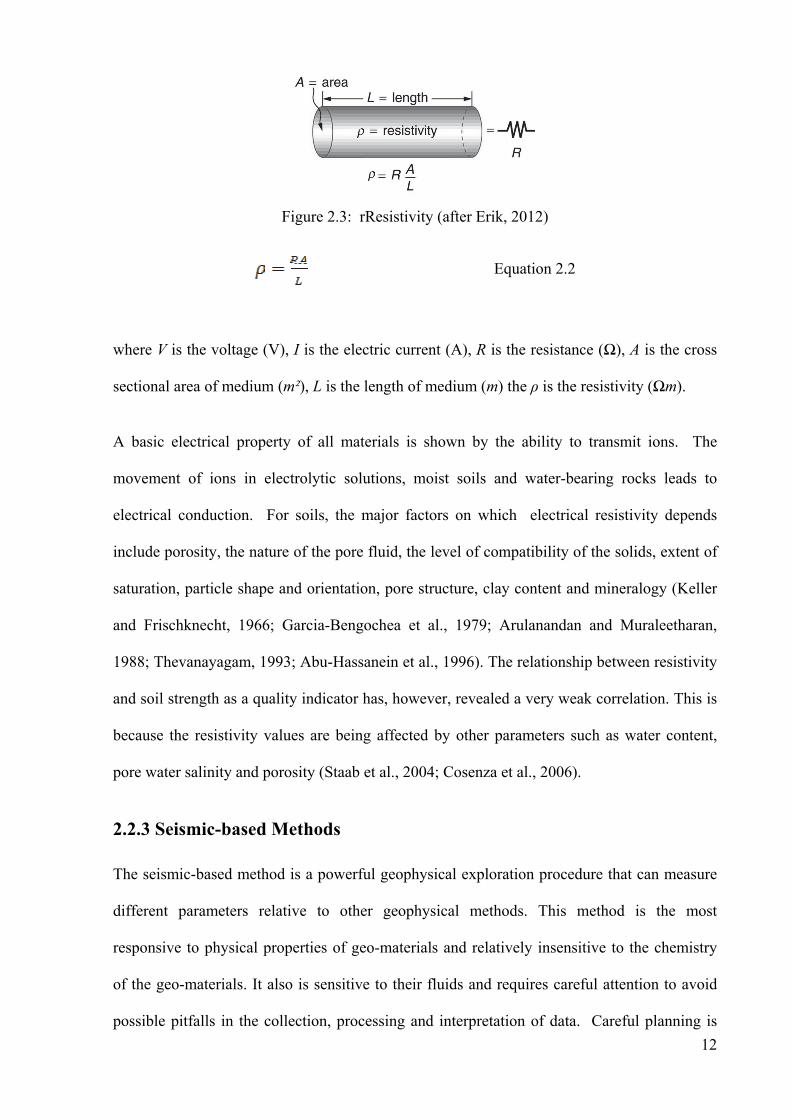
Figure 2.3: rResistivity (after Erik, 2012)
Equation 2.2
where V is the voltage (V), I is the electric current (A), R is the resistance (Ω), A is the cross
sectional area of medium (m²), L is the length of medium (m) the ρ is the resistivity (Ωm).
A basic electrical property of all materials is shown by the ability to transmit ions. The
movement of ions in electrolytic solutions, moist soils and water-bearing rocks leads to
electrical conduction. For soils, the major factors on which electrical resistivity depends
include porosity, the nature of the pore fluid, the level of compatibility of the solids, extent of
saturation, particle shape and orientation, pore structure, clay content and mineralogy (Keller
and Frischknecht, 1966; Garcia-Bengochea et al., 1979; Arulanandan and Muraleetharan,
1988; Thevanayagam, 1993; Abu-Hassanein et al., 1996). The relationship between resistivity
and soil strength as a quality indicator has, however, revealed a very weak correlation. This is
because the resistivity values are being affected by other parameters such as water content,
pore water salinity and porosity (Staab et al., 2004; Cosenza et al., 2006).
2.2.3 Seismic-based Methods
The seismic-based method is a powerful geophysical exploration procedure that can measure
different parameters relative to other geophysical methods. This method is the most
responsive to physical properties of geo-materials and relatively insensitive to the chemistry
of the geo-materials. It also is sensitive to their fluids and requires careful attention to avoid
possible pitfalls in the collection, processing and interpretation of data. Careful planning is
13
also necessary to make the method increasingly cost effective relative to test drilling and other
geophysical methods. The selection of seismic recording equipment, energy source and data-
acquisition parameters is often critical to the success of a project (Steeples and Miller, 1990).
The seismic-based techniques generally cause the ground to vibrate and produce very small
strains. Thus, the soil velocities derived from the seismic-based measurements are related to
the soil shear modulus. As such, seismic-based techniques can be used to directly derive the
geotechnical properties that relate to strain, including the maximum shear modulus (Gmax),
bulk modulus (B), Young’s modulus (E), and Poisson’s ratio (υ) (Steeples and Miller, 1990;
McDowell et al., 2002; Charles and Watts, 2002; Crice, 2005; Clayton, 2011).
In the seismic method, an elastic pulse or a more extended elastic vibration is generated at
shallow depth. The resulting motion of the ground at nearby points on the surface is detected
by small seismometers or “geophones”. The travel-time of the pulse to the geophones is
measured at various distances to obtain the velocity of transmission of the pulse in the ground.
Usually, the ground is not homogeneous in its elastic properties thus causing the velocity to
vary both laterally and in depth. In cases where the ground structure is simple, the values of
elastic wave velocity and the positions of boundaries between regions of different velocity can
be computed from the measured time intervals. Velocity boundaries usually coincide with
geological boundaries and the cross-section on which velocity interfaces are plotted. This may
be similar to the geological cross-section even though the two are not necessarily the same
(Griffiths and King, 1965).
In the fields of both engineering site investigation and hydrology, this seismic methodology
has been of considerable importance. The depth of interest ranges from approximately some
tens of metres to no more than a few hundred metres. The problems which may be solved
range from well-defined water table location or the estimation of the depth of high-velocity

14
“bedrock”, to the evaluation of the hydrological and mechanical properties including the
degree of saturation, the degree of fracturing, porosity, etc., of a concealed foundation
material aquifer (Griffiths and King, 1965).
2.3 Seismic Waves
There are different kinds of seismic waves and they all move in diverse ways. The two main
wave types are body waves and surface waves. While body waves can travel through the
earth's inner layers, surface waves on the other hand can only move along the surface of the
planet like ripples on water. Earthquakes usually radiate seismic energy as both body and
surface waves. A body wave is a combination of compression waves, which are called the P-
waves, and shear waves, which are called S-waves. A surface wave is a combination of
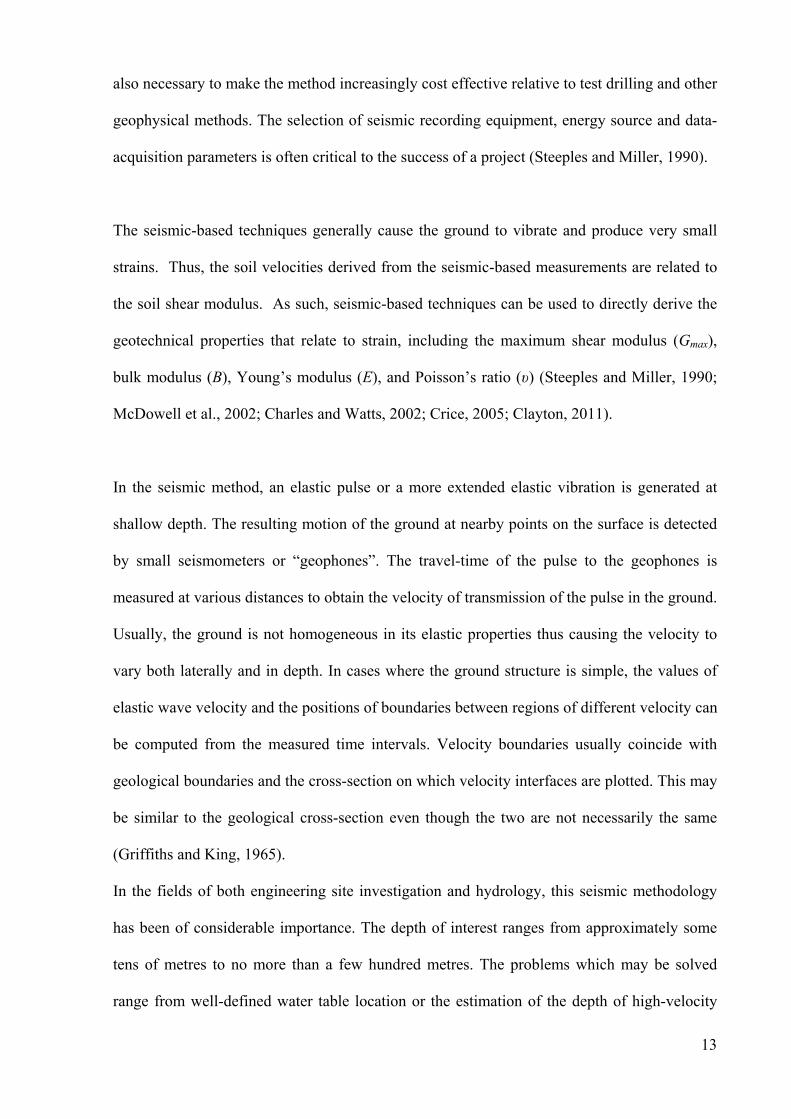
Rayleigh and Love waves, as shown in Figure 2.4. These four types of elastic seismic waves
are produced by impulses and all travel at different velocities (Michigan Technological
University, 2007).
When a sound wave travels in air, the molecules fluctuate forwards and backwards in the
direction of energy transport. Thus, this pressure or push wave travels as a series of refractions
and compressions. In a solid medium, the pressure wave has the highest velocity of any of the
possible wave motions and is then also known as the compression wave, primary wave or
simply P-wave (Milsom, 1939).
The vibration of particles at right angles to the direction of the energy flow creates an S-wave.
This is only possible in solids due to the relative low velocity. In many consolidated rocks, the
S-wave velocity is about half the P-wave’s velocity. This may depend slightly on the plane of
the vibrating particle, but such variations are usually inconsequential in small-scale surveys.
These kinds of waves are distortional stress waves that spread near to the ground surface with
15
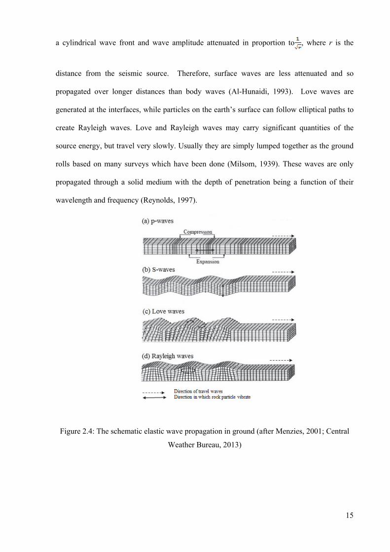
a cylindrical wave front and wave amplitude attenuated in proportion to , where r is the
distance from the seismic source. Therefore, surface waves are less attenuated and so
propagated over longer distances than body waves (Al-Hunaidi, 1993). Love waves are
generated at the interfaces, while particles on the earth’s surface can follow elliptical paths to
create Rayleigh waves. Love and Rayleigh waves may carry significant quantities of the
source energy, but travel very slowly. Usually they are simply lumped together as the ground
rolls based on many surveys which have been done (Milsom, 1939). These waves are only
propagated through a solid medium with the depth of penetration being a function of their
wavelength and frequency (Reynolds, 1997).
Figure 2.4: The schematic elastic wave propagation in ground (after Menzies, 2001; Central
Weather Bureau, 2013)
16
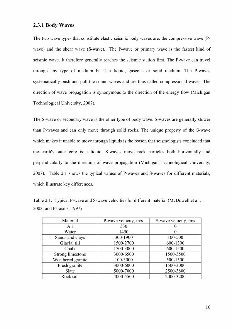
2.3.1 Body Waves
The two wave types that constitute elastic seismic body waves are: the compressive wave (P-
wave) and the shear wave (S-wave). The P-wave or primary wave is the fastest kind of
seismic wave. It therefore generally reaches the seismic station first. The P-wave can travel
through any type of medium be it a liquid, gaseous or solid medium. The P-waves
systematically push and pull the sound waves and are thus called compressional waves. The
direction of wave propagation is synonymous to the direction of the energy flow (Michigan
Technological University, 2007).
The S-wave or secondary wave is the other type of body wave. S-waves are generally slower
than P-waves and can only move through solid rocks. The unique property of the S-wave
which makes it unable to move through liquids is the reason that seismologists concluded that
the earth's outer core is a liquid. S-waves move rock particles both horizontally and
perpendicularly to the direction of wave propagation (Michigan Technological University,
2007). Table 2.1 shows the typical values of P-waves and S-waves for different materials,
which illustrate key differences.
Table 2.1: Typical P-wave and S-wave velocities for different material (McDowell et al.,
2002; and Parasnis, 1997)
Material P-wave velocity, m/s S-wave velocity, m/s Air 330 0
Water 1450 0 Sands and clays 300-1900 100-500
Glacial till 1500-2700 600-1300 Chalk 1700-3000 600-1500
Strong limestone 3000-6500 1500-3500 Weathered granite 100-3000 500-1500
Fresh granite 3000-6000 1500-3000 Slate 5000-7000 2500-3800
Rock salt 4000-5500 2000-3200

17
Refraction and reflection are the two most common types of seismic surveys that use body
waves. When a seismic wave meets an interface between two different types of rocks, some of
the energy is reflected while the residual energy is refracted at different angles. The law of
reflection is very simple and can be easily computed as being equal to the angle of incidence
(Figure 2.5a). The seismic refraction is based, fundamentally, on Snell’s Law (Equation 2.3),
which relates the angles of incidence and refraction to the seismic velocities in the two media.
sin i = V1/V2 Equation 2.3
where i is the critical incident angle (degree), V1 is the velocity of the upper layer (m/s) and V2
is the velocity of the lower layer (m/s).
Refraction will be towards the interface if V2 is greater than V1, and if sin i equals V1/V2 the
refracted ray will be parallel to the interface. In such a situation, part of the energy will return
to the surface as a head wave that leaves the interface at the original angle of incidence
(Figure 2.5 b). This is fundamentally how the refraction method works. If the incidence angle
is too large, then there will be no possibility of refraction and thus all the energy is reflected
(Milsom, 1939).
Figure 2.5: (a) Reflection from source 1 (S1) and (b) refraction from source 2 (S2) (after
Milsom, 1939).
When the seismic refraction method is used, it requires the soil layers to increase in density
with depth. Contrary to this, the reflection method requires the density contrast to reflect
18
waves back to the surface (Lankston, 1990). The travel time of the either the P-wave or S-
wave energy is recorded with the seismic refraction method. Therefore, by interpretation of
these data, the layer thicknesses and seismic velocities will be determined (McDowell et al.,
2002).
Traditionally, a small charge of dynamite is used as the common seismic source. Although
explosives are still quite commonly used to some extent, the use of impact and vibrator
sources have become popular in recent years. A simple sledge hammer provides a handy
source for small-scale surveys. The energy that is produced is useful and usually is reliant on
both the strength and skill of the operator as well as the ground conditions. Hammers can
nearly always be used in refraction work on spreads 10 to 20 m long but very seldom where
energy has to travel more than 50 m. More powerful impact sources are required for larger
surveys: for example, large weights of several hundreds of kilograms can be raised using
portable hoists and then dropped to create a larger source of impact. The use of vibration
sources is common when it involves large surveys that require extensive and complicated data
processing. Almost any type of safe explosive can be used for seismic work, but explosives
involve problems with safety, security and bureaucracy (Milsom, 1939).
There is considerable difference in the mode of generation of either a P-wave or an S-wave.
By using explosives or vertically dropping a mass into the ground, P-waves are automatically
generated. This makes the generation of P-waves easier than the generation of S-waves. S-
wave generation is more complex in that the energy needs to be induced in the ground
perpendicularly to the direction of the row of receivers. As a result, the soil particle motions
will be perpendicular to the direction of the wave propagation (Luna and Jadi, 2000). This
technique amplifies the S-wave amplitude while simultaneously decreasing the P-wave
amplitude, thus making the S-waves more easily identifiable in the seismic record (Lankston,
1990).

19
Instruments used for land seismic wave detection are called geophones, while those used in
the detection of waves under water are called hydrophones. They both convert mechanical
energy into electrical signals. Geophones are usually positioned by pushing a spike screwed to
the geophones into the ground or by using some form of adhesive pad or putty when working
on bare rock (Milsom, 1939).
By using the appropriate source for the waves and receivers, laboratory tests and field surveys
can be conducted using these two body waves. The time taken by the waves to travel from the
transmitter to the receiver is used to calculate wave velocities. The seismic waves can be
directly used to compute engineering properties. Using the P-wave and S-wave velocities, the
maximum shear modulus, Gmax, bulk modulus, B, Young’s modulus or dynamic elasticity
modulus, E, and Poisson’s ratio, υ, at varying small strains can be calculated using Equations
2.4 to 2.7 :
Equation 2.4
)21(32
υρν
−== EB p Equation 2.5
( ))1(
)1)(21(12
22
υυυρν
υρν−
+−=+= p
sE Equation 2.6
20
−
−
=
12
2
2
2
s
p
p
s
νν
νν
υ Equation 2.7
Where ρ is the bulk density of the soil (kg/m³), Vp is the P-wave velocity (m/s) and Vs is the S-
wave velocity (m/s) (Clayton et al., 1995; Menzies and Matthews, 1996; Massarsch, 2005).
The maximum shear modulus can be obtained from measurements of Vs alone by using
Equation 2.4 (Massarsch, 2005). Geo-materials have values of Poisson’s ratio in the range of
0.05 for very hard rocks and nearly 0.5 for saturated unconsolidated clays (Sheriff and
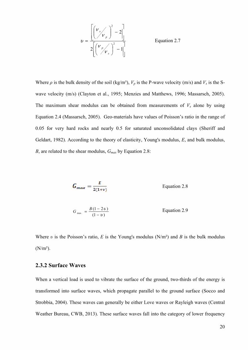
Geldart, 1982). According to the theory of elasticity, Young's modulus, E, and bulk modulus,
B, are related to the shear modulus, Gmax by Equation 2.8:
Equation 2.8
)1(
)21(max υ
υ−−= BG Equation 2.9
Where υ is the Poisson’s ratio, E is the Young's modulus (N/m²) and B is the bulk modulus
(N/m²).
2.3.2 Surface Waves
When a vertical load is used to vibrate the surface of the ground, two-thirds of the energy is
transformed into surface waves, which propagate parallel to the ground surface (Socco and
Strobbia, 2004). These waves can generally be either Love waves or Rayleigh waves (Central
Weather Bureau, CWB, 2013). These surface waves fall into the category of lower frequency
21
waves compared to body waves. They are easily differentiated on the seismogram regardless
of the fact that they arrive after body waves.
Love waves are named after the British mathematician A.E.H. Love, who worked out the
mathematical model for this kind of wave in 1911. Love waves are the fastest surface waves,
they move the ground from side-to-side and they produce entirely horizontal motion
(Michigan Technological University, 2007). The Rayleigh wave on the other hand was named
after John William Strutt Lord Rayleigh, who mathematically predicted the existence of this
kind of wave in 1885. Rayleigh waves result from the interfering P-waves and S-waves at the
ground surface (Xia et al., 2002). The way a Rayleigh wave rolls along the ground is similar
to how a wave rolls across a lake or an ocean. The fact that it rolls makes it capable of moving
the ground both horizontally and vertically perpendicularly to the wave motion.
Surface waves possess the property of dispersion and, therefore, can be used to categorize
near-surface elastic properties. This dispersive property comes about due to the fact that
different frequencies or wavelengths move at different depths (Reynolds, 1997). If a material
is homogeneous, then the surface wave velocity does not vary with frequency. However, if
the soil is heterogeneous with different densities, the surface wave velocity will fluctuate with
the frequency in areas where there is diversity in both stiffness and depth (Stokoe et al.,
1994). A graphical explanation of this phenomenon is illustrated in Figure 2.6, where
Medium 1 with thickness L overlies Medium 2. The Rayleigh wavelength (λ1) shorter than L
would propagate mainly within Medium 1, thus the phase velocity is representative of
Medium 1. However, the Rayleigh wavelength (λ2) is larger than L and this occurs when the
phase velocity is affected by the properties of both Mediums 1 and 2 (Rhazi et al., 2002). This
is a phenomenon known as dispersion, which thereby causes different frequencies and
wavelengths to travel at different velocities.

22
Figure 2.6: Rayleigh wave dispersion; Rayleigh wavelength (λ1) within Medium 1,
Rayleigh wavelength (λ2) within Medium 2 (after Rhazi et al., 2002)
The different ways of distinguishing surface waves vary according to the source and the field
receiver. Three major ways have been developed for site investigations using surface waves
and these are explained in detail in next sections. The first method makes use of a transient
vertical impact source and is known as the Spectral Analysis of Surface Waves (SASW)
method. The second uses a steady-state vibration source and is known as the Continuous
Surface-Wave (CSW) method (Sutton and Snelling, 1998). The third method uses multi-
channel receivers and either assorted active seismic sources such as sledge hammers or
ambient sources. This method is known as the Multi-channel Surface Wave (MSW) method
(Park et al., 2005).
2.3.2.1 Spectral Analysis of Surface Waves (SASW)
The Spectral Analysis of Surface Waves method was developed in the early 1980s, for
different engineering purposes. Compared to traditional borehole methods this allows for less
costly measurements while testing is performed on the ground surface. The basis of the
SASW method is the dispersive characteristic of Rayleigh waves when travelling through a
layered medium.

23
The Spectral Analysis of Surface Waves method uses a single pair of receivers that are placed
collinear with the impact point of the transient source. A series of hammer weights are
essential to create a range of frequencies – heavier weights are used to produce lower
frequency signals. To capture signals from ground motion receivers the SASW recordings use
a spectrum analyser, the signals usually being captured in the time domain and then converted
into the frequency domain. The phase difference between the signals from these spectral data
and the coherence of the cross-correlated signals at each geophone can be determined. The
coherence is a measure of the signal-to-noise ratio at a given frequency (Addo and Robertson,
1992).
SASW testing consists of obtaining and interpreting the corresponding shear wave velocity
profile through measuring the surface wave dispersion curve at the site. Surface waves are
generated by using a dynamic source wave of different wavelengths and are monitored by
multiple receivers at known offsets. Data from forward and backward profiles are averaged
together. An expanding receiver spread is used to avoid near-field effects associated with
Rayleigh waves. The geometry of the source receiver is used to minimize the body wave
signal. By using an interactive masking process, all the phase data are verified manually in
order to discard low quality data.
Figure 2.7 shows each step involved in the SASW method from data collection to data
analysis (Luke, 1999). Initially source energy is applied at the ground surface and then the
resulting ground motion is detected at the receivers and digitised at the analyser. The time
signals need to be transformed to the frequency domain and the phase difference between
receivers is determined. After that the phase data are unwrapped and the dispersion curve is
generated from the unwrapped, masked phase data at several different receiver spacings.
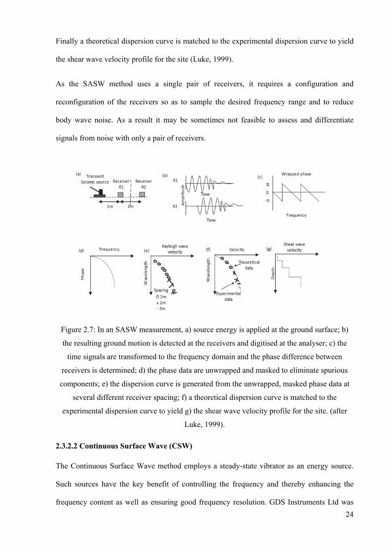
24
Finally a theoretical dispersion curve is matched to the experimental dispersion curve to yield
the shear wave velocity profile for the site (Luke, 1999).
As the SASW method uses a single pair of receivers, it requires a configuration and
reconfiguration of the receivers so as to sample the desired frequency range and to reduce
body wave noise. As a result it may be sometimes not feasible to assess and differentiate
signals from noise with only a pair of receivers.
Figure 2.7: In an SASW measurement, a) source energy is applied at the ground surface; b)
the resulting ground motion is detected at the receivers and digitised at the analyser; c) the
time signals are transformed to the frequency domain and the phase difference between
receivers is determined; d) the phase data are unwrapped and masked to eliminate spurious
components; e) the dispersion curve is generated from the unwrapped, masked phase data at
several different receiver spacing; f) a theoretical dispersion curve is matched to the
experimental dispersion curve to yield g) the shear wave velocity profile for the site. (after
Luke, 1999).
2.3.2.2 Continuous Surface Wave (CSW)
The Continuous Surface Wave method employs a steady-state vibrator as an energy source.
Such sources have the key benefit of controlling the frequency and thereby enhancing the
frequency content as well as ensuring good frequency resolution. GDS Instruments Ltd was

25
the first to utilise the Continuous Surface Wave System (CSWS; Sutton and Snelling, 1998).
This came as a huge step forward in site investigation technology. This system fundamentally
uses low natural frequency geophones to pick up surface waves that are generated by a
computer-controlled vibrator on the ground surface. This has enabled the creation of a ground
stiffness profiling system which is completely monitored by a computer. CSWS gives a
picture of the average maximum shear modulus (Gmax) with depth profile.
The seismic source uses a vibrator, which generates a number of continuous sinusoidal waves,
to produce surface wave frequencies in the range of 3Hz to 200Hz. A small electromagnetic
vibrator, weighing less than 15kg, is typically employed in order to obtain greater frequency
ranges and to facilitate mobility. [It is worth noting that such a vibrator is ineffective in giving
good quality sinusoidal waveforms when the frequencies are below 7Hz.] There is a need to
use heavier machinery to achieve lower frequencies in the range between 3Hz-50Hz. Longer
wavelengths are generated by lower frequencies and they penetrate further into the ground,
thus they can give a reasonable idea about deeper ground layers (Matthews et al., 1996).
It is possible to minimise the differences in the data by using many geophones, which allow
for a best fit line to be drawn through the phase angle-distance plot. It has been found that in
cases where two geophones are used, the results are unreliable. Therefore, in order to obtain
the best quality results, as many as 24 receivers are used as an evolution of the CSW
technique. Therefore, in order to establish the signal quality, a minimum of two sensors must
be used for the CSW test and must be arranged in a collinear fashion with the seismic source.
Figure 2.8 depicts a summary of the CSW technique. It starts with equipment preparation and
selective frequency (f1). This frequency sampling does not stop until n frequency (fn). Since
the captured data are in the time domain, they are converted to the frequency domain. As
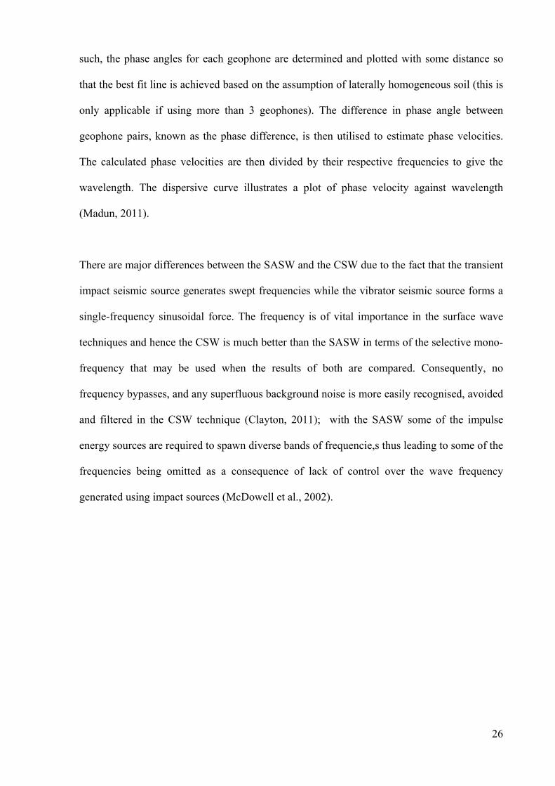
26
such, the phase angles for each geophone are determined and plotted with some distance so
that the best fit line is achieved based on the assumption of laterally homogeneous soil (this is
only applicable if using more than 3 geophones). The difference in phase angle between
geophone pairs, known as the phase difference, is then utilised to estimate phase velocities.
The calculated phase velocities are then divided by their respective frequencies to give the
wavelength. The dispersive curve illustrates a plot of phase velocity against wavelength
(Madun, 2011).
There are major differences between the SASW and the CSW due to the fact that the transient
impact seismic source generates swept frequencies while the vibrator seismic source forms a
single-frequency sinusoidal force. The frequency is of vital importance in the surface wave
techniques and hence the CSW is much better than the SASW in terms of the selective mono-
frequency that may be used when the results of both are compared. Consequently, no
frequency bypasses, and any superfluous background noise is more easily recognised, avoided
and filtered in the CSW technique (Clayton, 2011); with the SASW some of the impulse
energy sources are required to spawn diverse bands of frequencie,s thus leading to some of the
frequencies being omitted as a consequence of lack of control over the wave frequency
generated using impact sources (McDowell et al., 2002).
27
Figure 2.8: Schematic diagram showing the steps followed in the determination of the
dispersive curve using the CSW technique (after Matthews et al., 1996)
2.3.2.3 Multi-Channel Surface Waves (MASW)
One outstanding seismic method used for estimating ground stiffness or elastic state of the
soil is the Multi-channel Surface Wave (MSW) method, which was initially discovered in
Japan more than half a century ago. Initially it was called the micro-tremor survey method
(MSM). The Kansas Geological Survey in the late 1990s developed electrical equipment for
the MSW and used it for multi-channel analysis of surface waves, MASW (Park et al., 1999).
MASW operates by initially measuring the seismic surface waves obtained from various types
of seismic sources. The transmission velocities of these surface waves are then analysed to
deduce shear wave velocity variations below the surveyed area, which are related to its
geotechnical features.
28
Regular surface wave analysis approaches are based on a single transmitter-receiver pair in
contrast to the MSW, which brings in additional benefits as compared to conventional
methods. The MSW method is not affected by buried pipelines or cables, or by urban noise, to
the same extent as the seismic method that utilises body waves, because surface waves have
much bigger signals and are not constrained by the assumption inherent to seismic refraction
that the velocities increase with depth. On the other hand the use of a multiple-receiver
strategy for measuring has the advantage of shortening the time for the survey thus gives a
way for achieving lateral resolution, while the sub-surface characterisation in both the vertical
and lateral axes provides a convenient 2-D representation (Socco and Strobbia, 2004).
Generally, when the MSW method is used, all the seismic wave energy, both body and
surface waves, is recorded by the multi-channel receivers, which is the significant advantage
of MSW method.
MASW, which was presented by Park et al. (1999), allows one to efficiently identify, isolate
and filter noise from dispersed and reflected waves during data analysis just by using several
receivers and with only one shot. It therefore becomes possible for the best fit line to be drawn
on the phase angle plot. There are three main steps for the complete procedure of the MASW.
The initial step is obtaining the multi-channel field records. This is followed by the extraction
of the dispersion curves and finally inverting these dispersion curves to achieve a one- or two-
dimensional shear wave velocity and depth profile as shown in Figure 2.9.

29
When a pair of receivers is used in the SASW and CSW techniques, a one-dimensional result
of phase velocity against depth is obtained. It is of primary importance that a plot of the phase
velocity versus depth as a function of lateral distance is obtained in a lateral heterogeneous
medium. This aids the removal of all anomalies, thus rendering the MSW method more
effective than others. This method can be used to get an improved assessment of the
geotechnical features such as strength and stiffness because it provides relevant information in
the tangential dimension. This facilitates the detection of voids, fractures and soft spots
(Gordon et al., 1996).
2.4 Surface Wave Method
Data collection and signal processing are usually the two major steps used in spectral analysis.
With regard to data collection, a seismic source is generally used to generate a signal x(t), and
multiple receivers are deployed to acquire the seismic data. This is represented by y1(t)…yn(t),
where n is the index of the array of receivers. The familiar option for a seismic source is a
Figure 2.9. inverting the dispersion curves to obtain1-D or 2-D shear wave
velocity depth profiles (after Park et al., 2007 & 1999).

30
manually-controlled mass dropped to induce a broadband impulsive signal into the ground.
Another option could be the use of an electro-mechanical shaker that is generally controlled
by a digital source. The latter option makes it possible to vary and effectively adjust the
bandwidth and duration, and usually is relatively easy to implement. The receivers usually
consist of geophones for field testing, or accelerometers in laboratory-scale testing (Madun et
al., 2010).
The arrangement of the transmitter and receiver arrays is subject to the near- and far-offset
constraints (Heisey et al., 1982). These constraints are related to the signal wavelength and as
such they determine the highest and lowest frequencies that are relevant for spectral analysis.
As an empirical rule for the near-offset constraint it is recommended that the distance between
the source and the first receiver, dmin, as a function of the surface-wave wavelength, λ, is
approximated (Al-Hunaidi, 1993; Matthews et al., 1996; Park et al., 1999) using Equation
2.10:
Equation 2.10
When the receiver is far away from the seismic source, the far-offset is associated with the
attenuation of the surface waves. This constraint can be approximated by Equation 2.11:
minmax 2λ<d Equation 2.11
Furthermore, the spacing between the receivers, Δx, is given by Equation 2.12:
31
minλ≈Δx Equation 2.12
The wavelengths that pertain to both the smallest and highest frequencies are denoted by λmin
and λmax respectively.
The analysis used in such approaches assumes that the soil behaves as a layered half-space
that is laterally homogeneous and isotropic. Thus, the results represent the mean velocity of
the whole horizontal layer corresponding to the respective wavelength (Sutton and Snelling,
1998; Moxhay et al., 2001; Moxhay et al., 2008; Redgers et al., 2008; Roy, 2010).
2.5 Relationship of Seismic to Geotechnical Parameters
Seismic waves or elastic stress waves travelling through soils interact with soil particles and
interstitial fluids. So seismic wave responses are affected by the soil texture and structure, and
they are sensitive to the variations in soil properties. Propagation of seismic waves through
soils is a small-strain phenomenon that introduces a small perturbation without altering the
fabric of the soil. As a result, seismic parameters are constant fabric characteristics and can be
used to estimate and observe on-going internal changes of soil properties.
The resistance of the body to deform under applied force is termed stiffness (Clayton, 2011).
So when a body is being referred to as being stiff, it can be inferred that it is difficult to easily
deform it when a force is applied to it. The three stiffness parameters are known as Young’s
modulus, E, bulk modulus, B, and shear modulus, G.
Atkinson states that the relationship between strain and stiffness of soils is generally non-
linear and only at very small strains does the correlation between strain and stiffness behave in
a linear fashion. It is at these smaller strains that the shear stiffness reaches its maximum
value, usually referred to as G0 or Gmax (Atkinson, 2007).
32
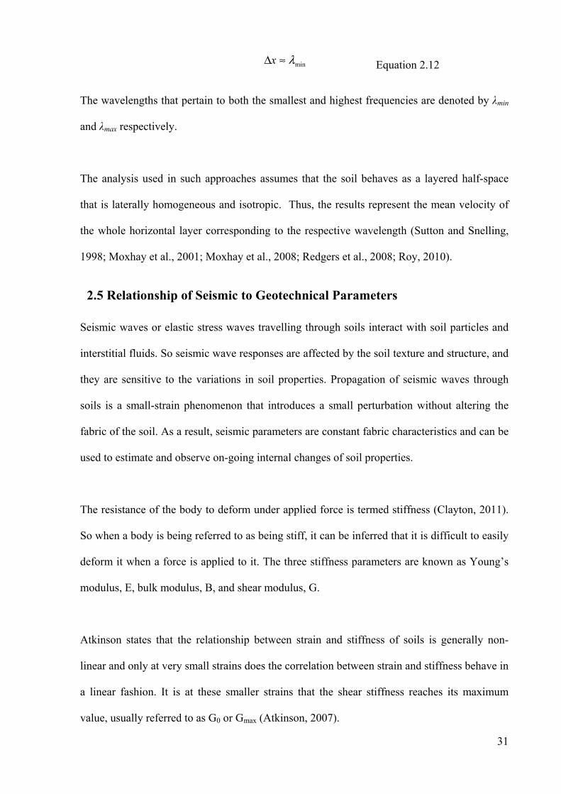
In summary the material’s maximum modulus depicts the modulus value over the linear
section of stress-strain curve and is popularly symbolized as Emax, maximum Young’s
modulus, or Gmax, the maximum shear modulus. Figure 2.10 gives a clear picture of this
relationship.
Figure 2.10: Modulus variations with strain level (after Davich et al., 2004)
Measurement of soil stiffness parameters is made by conducting stress path triaxial tests in the
laboratory, since in the conventional triaxial test it is unreliable to measure strain smaller than
0.1%. However, using the hydraulic triaxial test it is possible to measure strain smaller than
0.01%. To achieve 0.001% strain reliably, an internal strain gauge should be mounted
directly on the sample. It is very difficult to measure stiffness of soil at very small strain, i.e.
less than 0.001%, using triaxial tests by direct measurement of strains. However, the simplest
way is to measure and calculate shear modulus at very small strain using the seismic shear
wave velocity (Atkinson, 2007). Another way to obtain small strain moduli is by using bender
elements. They are usually short piezoelectric cantilever strips that have direct contact to the
specimen. Although there are several different types of bender elements, the fundamental
concept of each of the apparatuses does not change. On opposite sides of the soil specimen,
two small elements are inserted. By using the piezoelectric material to generate motion, an

33
electric pulse is sent to one of these elements which ultimately produces compression (P) or
shear (S) waves in the soil. These waves depend upon the direction of the piezoelectric
material. Figure 2.11 shows a schematic of this process. As the bender element on the
opposite side receives the wave, a time path is documented. It thus becomes possible to
calculate the Poisson’s ratio and the shear modulus of the soil being tested when both the
shear and compression waves have been identified (Davich et al., 2004).
Figure 2.11: Bender element wave generation (after Davich et al., 2004)
The soil moduli generated from both the seismic and geotechnical testing is at different strain
levels. The basic difference between both strains is that those from the seismic waves are
caused by very low range vibration of soil particles, meanwhile strains from geotechnical
testing in the triaxial test range from 0.01 to 0.001% (Matthews et al., 2000). Differences in
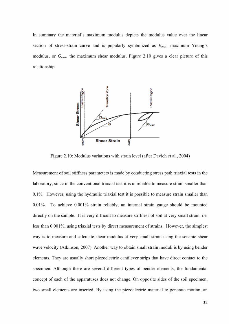
strain dimension can be prone to faulty correlations. Figure 2.12 illustrates the way in which
Atkinson (2007) abridged the relationship between the stiffness or the shear modulus and the
strain. It can be seen that as the soil stiffness or the shear modulus decreases, as the strain
increases. The three principal regions of soil stiffness are very small strains, small and large
strains. The value of the first strain region generates up to a 0.001% strain reaches the highest
approximately constant value. For the small strain region (i.e. the second or intermediate
region), the shear modulus rapidly decreases in a non-linear way with increasing strain. In the
large strain region, the soil state has reached the state boundary surface and the soil behaviour
is elasto-plastic and it is usually greater than 1 %.
34
Figure 2.12: Characteristic ranges of soil stiffness modulus
(after Atkinson, 2007).
As mentioned before there are three stiffness parameters; Young’s modulus, E, bulk modulus,
B, and shear modulus, G. Fundamental differences exist between all three types of moduli.
The key characteristic of the Young’s modulus is that it comprises both the volumetric strains
and shear distortion. The bulk modulus on the other hand is composed of strain modifications
in volume with no variations in the shape. On the other hand, the shear modulus is determined
when the strain change is due to changes in shape but no alterations in volume (Menzies and
Matthews, 1996).
Some researchers like Mattsson et al. (2005) and Chan (2006) showed that there is a close
relationship between the stiffness parameters (Young’s modulus, E, bulk modulus, B, and
shear modulus, G) determined from seismic tests and other soil parameters such as soil
strength, for example. Soil parameters such as soil strength showed a high correlation between
the maximum soil modulus (Gmax) and undrained shear strength (cu) of stabilised clay (Chan,
2006).
2.6 Experimental Relationships and Data from the Literature
Baxter and Sharma (1977), commenting that changes in Gmax or vs during shearing have been
studied for clayey soils (e.g. Rampello et. al., 1997; Teachavorasinskun and
35
Amornwithayalax, 2002; Teachavorasinskun and Akkarakun, 2004), presented the variation
of shear wave velocity, vs, during shear. In their research, drained and undrained triaxial tests
on cemented sands were performed with shear wave velocity measurements throughout the
shearing process. The results showed that shear wave velocity during shear does not depend
solely on mean normal effective stress (p′). During drained shear, vs was found to be
dependent on σ′1 and during undrained shear vs was dependent on σ′3 . During drained shear, vs
peaks before the strength of the soil is fully mobilized, and this feature of vs can be used as an
indicator of bond breakage in cemented soils. For cemented soils the vs behaviour during shear
is not well represented by a power law function of p′.
Yunmin et al. (2005) studied the correlation of shear wave velocity with liquefaction
resistance based on laboratory tests. A simplified procedure is proposed based on the
combination of in situ measurements of shear wave velocity and laboratory tests for
evaluating liquefaction resistance and other factors such as relative density. Two series of
dynamic triaxial tests were devised: (1) control of the shear wave velocity by changing the
relative density or strain history with the confining stress (100kPa) unchanged; and (2) control
the shear wave velocity by changing its confining pressure with the relative density (60%)
unchanged. Bender elements were installed on samples tested using the conventional dynamic
triaxial tests system, so that both measurements of shear wave velocity and dynamic triaxial
tests could be conducted consecutively on the same samples. The generation and receiving of
the shear wave are carried out by the bender elements, which were then used to determine the
shear-wave velocity. The sands used in these tests were obtained from two sites in China:
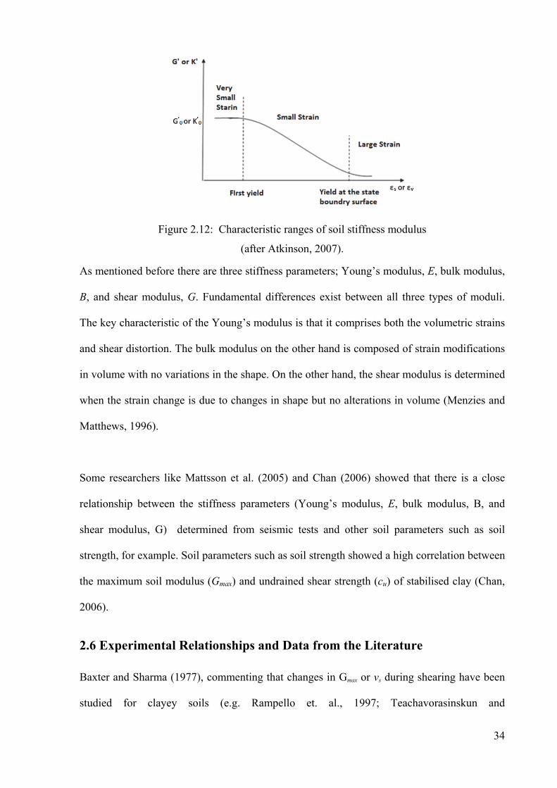
Hangzhou and Fujian. Furthermore, these authors referred to a case study by Andrus and
Stokoe (2000) about a site at Treasure Island Fire Station, in California, where the value of
shear wave velocity measured by cross-hole testing, assuming soil density of 1.76Mg/m3, was
found to be between 140-200m/s. ( see figure 2.13)

36
Figure 2.13 variation of shear wave velocity with depth (Yunmin et al. (2005))
Molnar et al. (2007) compared geophysical shear-wave velocity methods. The methods
examined included both invasive (SCPT: Seismic cone penetration tests), and non-invasive
techniques, including both active (SASW: Spectral Analysis of Surface Waves and CSWS:
Continuous Surface Wave System), and passive sources (the single-instrument microtremor
method). They concluded that sites with relatively soft soil are generally investigated with
SCPT method while for sites which are too dense for cone penetration, SASW and CSWS
methods were employed. They report a range of values for different geological horizons: for
example, based on the 21 SCPT and 4 SASW field tests, a shear-wave velocity model has
been determined by Monahan and Levson (2001) for bedrock in Greater Victoria, which
consists of igneous and metamorphic rocks (Nasmith and Buck, 1998); the bedrock is
estimated to have high shear-wave velocities of 1000-2500m/s (see also Hunter et al., 1999).
They report the average shear-wave velocity of other geological units as follows: till and over-
consolidated sediments earlier than the last glaciation, 390-550 m/s ; Colwood sand and
gravel, 270-380m/s ; Colwood delta slope, 150-230m/s; brown Victoria clay, 160-260 m/s ;
grey Victoria clay 100-160m/s ; and Holocene organic soils, 40-100m/s.
37
Uyanil (2011) studied the porosity of saturated shallow sediments from seismic compressional
and shear wave velocities. This study presents a new analytical relationship between Poisson's
ratio and shear modulus values, which were obtained from seismic velocities and porosity
values of water-saturated material computed from water content and grain densities, which
were determined by laboratory analysis of disturbed samples. The aim of the study was to
estimate the porosity of water-saturated undrained soils without obtaining samples or
disturbing the natural situation of soils, and this was achieved by using a nondestructive
seismic refraction method to determine the seismic wave velocities. The analytical
relationship between data sets indicates that when the shear modulus of water-saturated loose
soil increases, porosity decreases logarithmically. If shear modulus increases in dense or solid
saturated soils, porosity decreases linearly. This research indicates that porosity is one of
several factors affecting the propagation of seismic waves in soils; other factors are: 1.
Lithological properties of soil (grain sizes, shape, type, distribution, amount, compaction,
consolidation and binding); 2. Physical properties (porosity, permeability, density, anisotropy,
saturation degree, solid–liquid interference, pressure and temperature); and 3. Elastic
properties (shear modulus (G), bulk modulus (K), Young modulus (E), Poisson's ratio (μ) and
Lamé constant (λ)). Any change in the lithological properties of soil also affects seismic wave
velocities, e.g. the higher the compaction rate the higher the velocities of both shear waves (S-
waves) and compressional waves (P-waves). These relationships have been the
Pickett (1963) showed that the ratio of compressional (P) to shear (S) wave velocities could
serve as a lithological indicator. The velocity of seismic waves changes according to the
physical properties of soils; the seismic wave velocity in dense soil is higher than that in loose
soil (Uyanık and Ulugergerli, 2008). Increasing soil density indicates higher soil compaction.
P-wave velocity is therefore utilized in identifying lithology, porosity and pore fluids. S-wave
velocity is utilized for mineral identification, determining soil porosity and for identifying

38
fluids. Hardin and Black (1968), and Hardin and Drnevich (1972), established experimental
relationships between void ratio and shear modulus.
The development of the analytical relationship derived for this research indicates dependency
of the bulk modulus (K) on shear modulus (G) and Poisson's ratio (μ), and then the shear
modulus (G) is related to shear wave velocity (vs), density (γ) and gravitational acceleration
(g). Lastly, Poisson's ratio (μ) is related to vs and vp. In Uyanik’s (2011) study, seismic P- and
S-waves were recorded using vertical and horizontal component geophones respectively,
connected to a 12-channel analogue recorder. Geophones were firmly attached to the ground
and the first break arrival time of direct and refracted waves was obtained by digitizing and a
commercial software package, SeisOPT® (Pullammanappallil and Louie, 1993). The results
of the 2D inversion of the first arrivals for each profile were thus obtained. Geo-seismic
sections (velocity-depth profiles, see figure 2.14) were determined as variations in velocities
with respect to distance and depth. From these variations in velocities, the average seismic
compressional and shear wave velocities were obtained. These average velocities were used in
geotechnical cross-sections. The samples used for this research were classified as gravely,
sandy and clayey-silty soils. Generally, shear wave velocity was found to increase slightly
with depth in the studied sediments and water content decresase with depth (see figure 2.14).
In the gravel soils, shear wave velocity lay within the range 66–503m/s (average 260m/s),
while in sandy soils the shear velocities were within the range 105-516m/s (average 294m/s)
and in the clayey–silty soils shear wave velocity fell within the range 58-584m/s (average
264m/s). (see table 2.2)

39
Table 2.2 minimum maximum and mean values of measure shear wave velocity in gravel, sand and clay-silt (Uyanik’s (2011))
Soil type gravel Sand Clay-Silt
a b c d e f g h i j k l
Shear wave velocity
169 138 66 126 165 332 155 105 177 134 78 58 Min
503 460 441 357 507 516 428 356 584 562 437 420 Max
300 283 244 212 328 440 265 144 370 352 172 162 Ave.
Maheswari et al. (2008) studied the development of empirical correlation between shear wave
velocity and standard penetration resistance in soils of Chennai city. They indicated that
knowledge of accurate and realistic dynamic characteristics, such as shear wave velocity and
other related dynamic soil properties like shear modulus, damping ratio, etc., is an essential
requirement in the analysis of seismic wave propagation. In Chennai city, the soil formation
mainly consists of soft marine clay, stiff clay and loose sand. In their study Multichannel
Analysis of Surface Wave (MASW) tests were carried out using a seismic recorder with 24
vertical geophones, which were used to receive the wavefields generated by the active source
of a sledgehammer. In order to have a confidence on the obtained shear wave velocities from
MASW test, a seismic cross-hole test and bender element tests have also been carried out and
the results from all methods match well. Their results show that in general shear wave
Figure 2.14 distribution of shear and compresional wave velocity and water content with depth (Uyanik’s (2011))
40
velocity increased slightly with depth (0-16m) and the shear wave velocity was within the
range 150-250m/s.
Thitimakorn (2010) compared shear-wave velocity profiles of Bangkok subsoils from Multi-
Channel Analysis of Surface Wave and down-hole seismic methods.
This study compares estimates of vs derived from the traditional borehole method with those
derived from the newer MASW technique at three sites near Bangkok, Thailand, namely at
the Asian Institute of Technology (AIT), Chulalongkorn University (CU) and the Thailand
Metrological Department (TMD). The Bangkok subsoil is reasonably uniform throughout the
entire region and consists of marine and terrestrial deposits, the uppermost layer being known
as Bangkok soft clay. All the results indicate that the MASW technique was acceptably
congruent with the standard downhole seismic technique and therefore the MASW method
was considered acceptable for estimating vs of soils in and around the Bangkok area. The
results shows the average shear wave velocity was between 150-300m/s by MASW method
and 100-260m/s from the traditional borehole method at these three sites near Bangkok.
These finding are put into context by the work of Ashford et al. (1997), who reported that the
shear-wave velocity (vs) of the Bangkok soft clay layer was really low (about 60 to 100m/s),
whilst that for the underlying stiff clay layer was in the range of 150-200 m/s, increasing to
about 250 m/s for the first layer beneath that. He also stated that the low shear-wave velocity
of Bangkok clay is comparable to Mexico City clay.
Adamo et al.,(2009), have presented the theoretical basis and practical; experimental setup for
measuring the water content. The soil specimen used to perform the experiments was sandy
soil and it was contained in a reinforced wood box measuring 170cm× 90 cm ×80cm
(L×W×H). The compressional and shear waves velocities have been measured for four
different values of the saturation ( 0.6%,30%,50%, and 70%). The theoretical analysis shows

41
that by measuring the shear waves velocity it is possible to estimate the water content, and the
velocities ratio gives information about water distribution into the examined soil. The
experimental setup has produced results in a good agreement with the theoretical values. The
measured values of velocities reported, ranging from 130 to 150 m/s in case of compression
wave and from 80 to 90 m/s in case of shear wave for sandy soil specimen.
Adamo et al., (2004), also have shown that by introducing suitable simplifications and
hypotheses in the equations of elastic waves propagation of compressional waves and the
moisture content of soil can be obtained. But this approach had some limitations a good
knowledge of many parameters of the medium (e.g., porosity, density, granular composition,
etc) are required.
They also have studied the possibility of using shear waves velocities in conjunction with
compressional ones.
Madun et al., (2012), describes a methodology for performing surface wave testing in the
laboratory. In comparison with field tests, a laboratory-scale experiment offers the advantage
of allowing the process of data collection to be calibrated, and analytical studies can be
carried out as the properties of the material under test are controllable and known a priori. In
addition, a laboratory scale experiment offers insight into the interaction between the seismic
surface wave, the soil, the boundary and, hence, the constraints associated with the seismic
surface wave technique.
Two simplified models of different sizes were developed using homogeneous remoulded
Oxford Clay at different water contents and corresponding undrained shear strengths. In this
setup, two sizes of containers were constructed measuring (1): 600 mm x 300 mm x 300 mm
and (2): 1080 mm x 680 mm x 500 mm in length, width and depth respectively. The
The measured phase velocities were converted to shear wave velocities using equation and the
the maximum shear modulus, G , was calculated using equation Gmax=ρ(density)×v2(shear
containers contained Oxford Clay at different water contents of 32 % and 40 %.
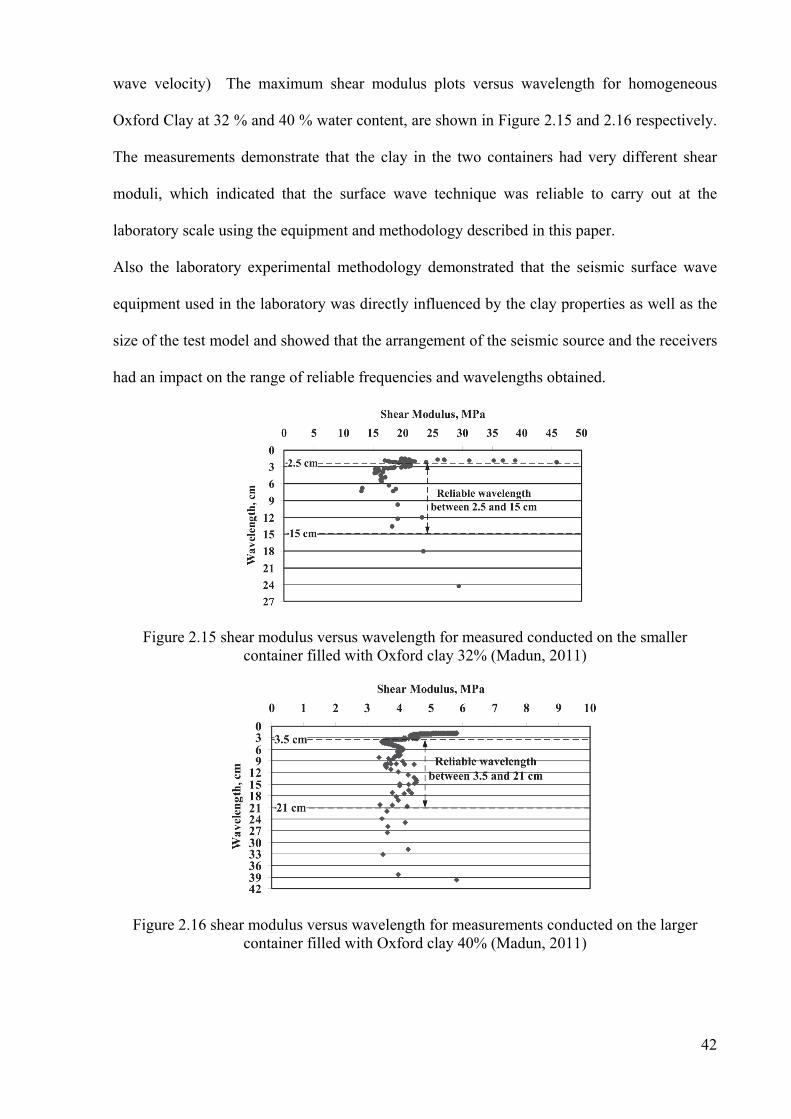
42
wave velocity) The maximum shear modulus plots versus wavelength for homogeneous
Oxford Clay at 32 % and 40 % water content, are shown in Figure 2.15 and 2.16 respectively.
The measurements demonstrate that the clay in the two containers had very different shear
moduli, which indicated that the surface wave technique was reliable to carry out at the
laboratory scale using the equipment and methodology described in this paper.
Also the laboratory experimental methodology demonstrated that the seismic surface wave
equipment used in the laboratory was directly influenced by the clay properties as well as the
size of the test model and showed that the arrangement of the seismic source and the receivers
had an impact on the range of reliable frequencies and wavelengths obtained.
Figure 2.15 shear modulus versus wavelength for measured conducted on the smaller container filled with Oxford clay 32% (Madun, 2011)
Figure 2.16 shear modulus versus wavelength for measurements conducted on the larger container filled with Oxford clay 40% (Madun, 2011)
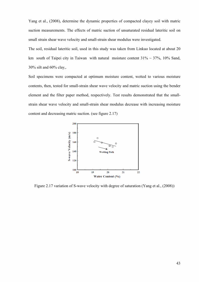
43
Yang et al., (2008), determine the dynamic properties of compacted clayey soil with matric
suction measurements. The effects of matric suction of unsaturated residual lateritic soil on
small strain shear wave velocity and small-strain shear modulus were investigated.
The soil, residual lateritic soil, used in this study was taken from Linkuo located at about 20
km south of Taipei city in Taiwan with natural moisture content 31% ~ 37%, 10% Sand,
30% silt and 60% clay,.
Soil specimens were compacted at optimum moisture content, wetted to various moisture
contents, then, tested for small-strain shear wave velocity and matric suction using the bender
element and the filter paper method, respectively. Test results demonstrated that the small-
strain shear wave velocity and small-strain shear modulus decrease with increasing moisture
content and decreasing matric suction. (see figure 2.17)
Figure 2.17 variation of S-wave velocity with degree of saturation (Yang et al., (2008))
44
2.7 Summary
This chapter summarised the advantages of seismic-based techniques compared with other
geophysical and geotechnical techniques. The seismic wave results are directly related to
active soil properties such as the maximum shear modulus, Gmax, the bulk modulus, B,
Young’s modulus, E, and Poisson’s ratio, ʋ (Charles and Watts, 2002; Crice, 2005).
Seismic-based methods have been proven to be both more versatile than other methods as
well as being more economical in terms of field operation to determine physical properties of
tested geo-materials (Matthews et al., 2000). Since the surface waves travel in the vicinity of
the ground surface, they are less attenuated and dispersive. The dispersive features pertains
uniquely to the surface wave in which case the frequency and wavelength change as a result
of the different velocities when the soils are layered. The dispersive phenomenon is used to
identify the soil properties with depth. SASW, CSW and MSW are common surface wave
techniques. Of all these techniques, MSW is preferred due to its flexibility in the signal
processing approach to extract the dispersion curve.

45
Chapter 3
INITIAL TESTING METHOD
3.1 Introduction
In this section, emphasis is placed on the development of small-scale seismic surface wave
testing in the laboratory as well as assessing the viability of the proposed method to
investigate the relationship between the geophysical and geotechnical properties of soil, so
that geotechnical soil databases can be used to inform geophysical surveying protocols and
results analysis.
The choice of which geophysics tests to use depends on the parameters to be examined
(Mitchell and Jardine, 2002). Amongst geophysical methods, the seismic method based
results empirically derive geotechnical properties such as maximum shear modulus ( )maxG ,
bulk modulus (B), Young’s modulus (E), and Poisson’s ratio ( )υ (Charles and Watts, 2002;
Crice, 2005) and the seismic-based techniques have proved particularly useful in determining
shear modulus which can be expand to calculate the shear wave velocity and find that how
soil properties influence acoustic wave transmission during the seismic surface wave testing
(Moxhay et al., 2001; Redges et al., 2008).
46
As testing in the field is difficult and complex, and this is coupled with non-homogeneity of
typical natural ground conditions, the laboratory test was established to provide a
straightforward means of creating repeatable data and the process was further simplified by
the use of homogeneous material. The outcomes from testing can be then used to develop
procedures for full seismic testing in natural soil as part of supplementary work
The selection of seismic sources was determined by the level of frequency and energy
required for the test materials and the selection of the seismic apparatus, specification and the
size of the test models has to consider the factors of time, cost and workability. The seismic
surface wave equipment for use in the laboratory seismic tests was directly related to the
material properties and the size of the test model.
The development of the small-scale model for seismic surface wave testing in the laboratory
aimed to develop the most appropriate seismic surface wave method for attaining and utilising
the data to investigate the influence of soil properties on acoustic wave transmission
To achieve this aim, it is necessary to investigate the suitability of the seismic equipment and
its system for laboratory use. The use of seismic surface wave methods in the laboratory
should have sufficient sample volume size to reduce the effect of seismic wave back-
scattering, due to the model boundary together with interference by body waves.
Kaolin Clay and Oxford Clay were used for these tests, Oxford Clay being more practically
relevant than Kaolin since Oxford Clay is representative of natural soil. This is because
Oxford Clay has various clay types and hence a mixed mineralogy. Use of Kaolin Clay,
which is a pure form of kaolinite, ensures a high degree of sample control, simplifies the
analysis and reduces variability throughout the test programme. Laboratory-scale experiments
are preferable over field tests because the data collection process occurs under far more
controlled conditions to obtain the true measure of the data that are being collected.
47
3.2 Establishing Laboratory Seismic Surface Wave Equipment
The most relevant factors that were vital for the success of the seismic surface wave tests in
the laboratory can be seen in Figure 3.1. In essence, there are two major pieces of apparatus
for the seismic test, namely the seismic source, which generates vertical ground motions using
a point source of energy, and the seismic recorder. To have more flexibility in the size of the
test model, a high frequency range for the seismic receivers was selected.
To investigate correlation between the geophysical and geotechnical properties of soil,
development of the most appropriate small-scale model for laboratory seismic surface wave
testing is necessary both in terms of obtaining and utilising the data. The effect of seismic
wave back-scattering needs to be reduced, so the laboratory seismic surface wave method
chosen should have sufficient sample volume size. This is mainly because the model is bound
to interfere with body waves which then intensify the signal-to-noise ratios.

48
This research uses two different types of soils, i.e. Kaolin and Oxford Clay. For laboratory
testing, the equipment and its systems need to be appropriate to determine change of soil
properties, and hence the suitability of the seismic source-receivers array should be
considered. A summary of the overall testing, involving a variety of materials and how they
related to one another, is shown in Figure 3.2. In this chapter the initial test methods are
discussed, while the corresponding results are presented in Chapter 4. Afterwards, the main
test methodology is discussed in Chapter 5 and the associated results presented in Chapter 6.
Figure 3.1: The seismic surface wave factors that contributed to the success of tests at the
laboratory scale.
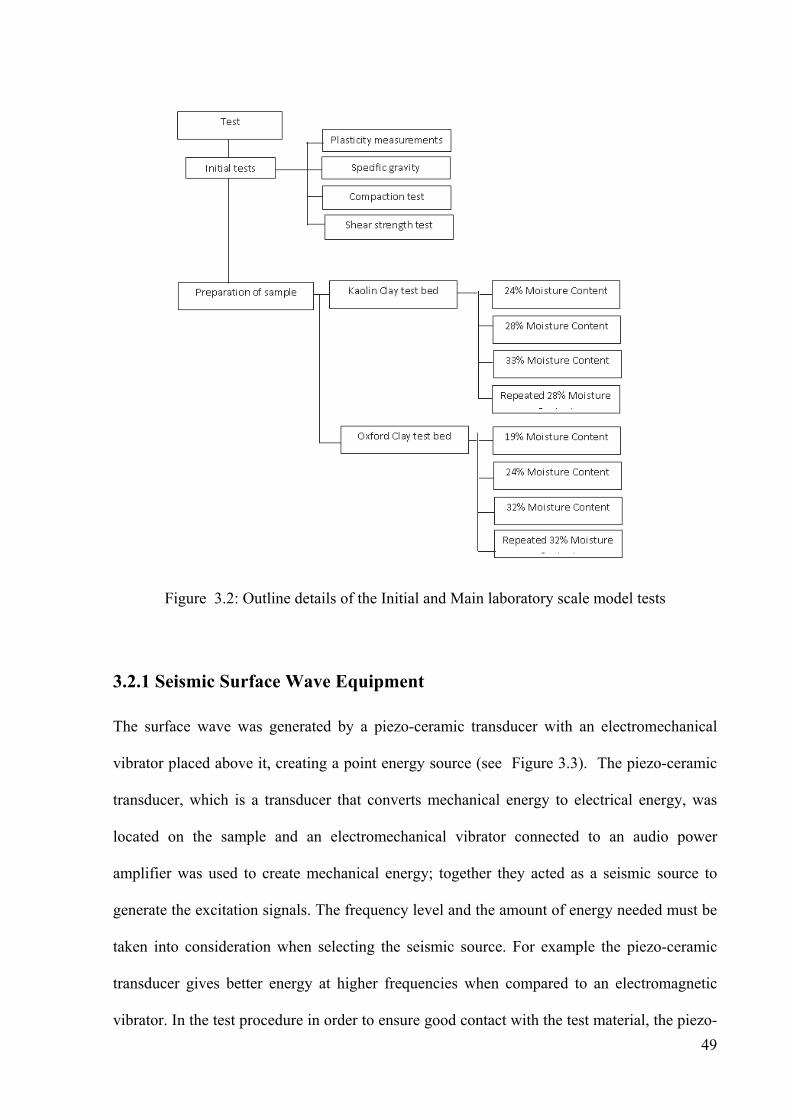
49
Figure 3.2: Outline details of the Initial and Main laboratory scale model tests
3.2.1 Seismic Surface Wave Equipment
The surface wave was generated by a piezo-ceramic transducer with an electromechanical
vibrator placed above it, creating a point energy source (see Figure 3.3). The piezo-ceramic
transducer, which is a transducer that converts mechanical energy to electrical energy, was
located on the sample and an electromechanical vibrator connected to an audio power
amplifier was used to create mechanical energy; together they acted as a seismic source to
generate the excitation signals. The frequency level and the amount of energy needed must be
taken into consideration when selecting the seismic source. For example the piezo-ceramic
transducer gives better energy at higher frequencies when compared to an electromagnetic
vibrator. In the test procedure in order to ensure good contact with the test material, the piezo-
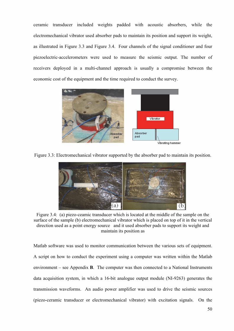
50
ceramic transducer included weights padded with acoustic absorbers, while the
electromechanical vibrator used absorber pads to maintain its position and support its weight,
as illustrated in Figure 3.3 and Figure 3.4. Four channels of the signal conditioner and four
piezoelectric-accelerometers were used to measure the seismic output. The number of
receivers deployed in a multi-channel approach is usually a compromise between the
economic cost of the equipment and the time required to conduct the survey.
Figure 3.3: Electromechanical vibrator supported by the absorber pad to maintain its position.
Figure 3.4: (a) piezo-ceamic transducer which is located at the middle of the sample on the
surface of the sample (b) electromechanical vibrator which is placed on top of it in the vertical direction used as a point energy source and it used absorber pads to support its weight and
maintain its position as
Matlab software was used to monitor communication between the various sets of equipment.
A script on how to conduct the experiment using a computer was written within the Matlab
environment – see Appendix B. The computer was then connected to a National Instruments
data acquisition system, in which a 16-bit analogue output module (NI-9263) generates the
transmission waveforms. An audio power amplifier was used to drive the seismic sources
(piezo-ceramic transducer or electromechanical vibrator) with excitation signals. On the
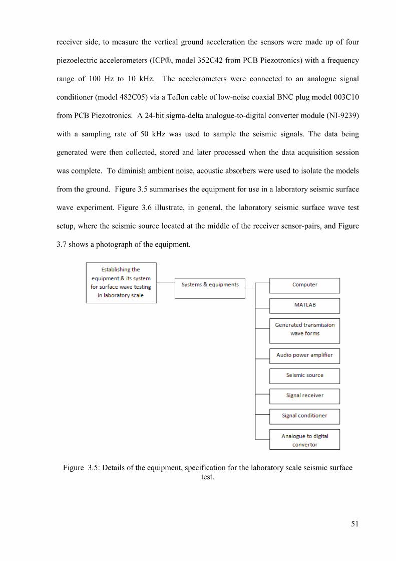
51
receiver side, to measure the vertical ground acceleration the sensors were made up of four
piezoelectric accelerometers (ICP®, model 352C42 from PCB Piezotronics) with a frequency
range of 100 Hz to 10 kHz. The accelerometers were connected to an analogue signal
conditioner (model 482C05) via a Teflon cable of low-noise coaxial BNC plug model 003C10
from PCB Piezotronics. A 24-bit sigma-delta analogue-to-digital converter module (NI-9239)
with a sampling rate of 50 kHz was used to sample the seismic signals. The data being
generated were then collected, stored and later processed when the data acquisition session
was complete. To diminish ambient noise, acoustic absorbers were used to isolate the models
from the ground. Figure 3.5 summarises the equipment for use in a laboratory seismic surface
wave experiment. Figure 3.6 illustrate, in general, the laboratory seismic surface wave test
setup, where the seismic source located at the middle of the receiver sensor-pairs, and Figure
3.7 shows a photograph of the equipment.
Figure 3.5: Details of the equipment, specification for the laboratory scale seismic surface test.

52
Figure 3.6: Laboratory setup for seismic surface wave test.
Figure 3.7: (a) Signal conditioner, (b) Signal amplifier, (c) Data acquisition system, (d) Piezo-transducer, (e) Piezo-electric accelerometer, (f) Teflon cable, (g) Electromechanical
vibrator
Rayleigh waves will be formed when the wavelength is smaller than half of the model depth
(Zerwer et al., 2000 and 2002). As the piezo-ceramic transducers are suitable for transferring
high frequency energy they are most appropriate for the clay model, which requires a higher
frequency. The excitation signal was generated by using an audio power amplifier to drive the
piezo-ceramic transducer and, as stated above, the piezo-ceramic transducer was acoustically
coupled to the surface with the use of a weight padded with acoustic absorber. In view of the
fact that the frequency range of the accelerometers is up to 10 kHz, the captured data will not
exceed 10 kHz. Figure 3.8 shows the laboratory-scale model and equipment setup on the clay
model with sensing accelerometers.
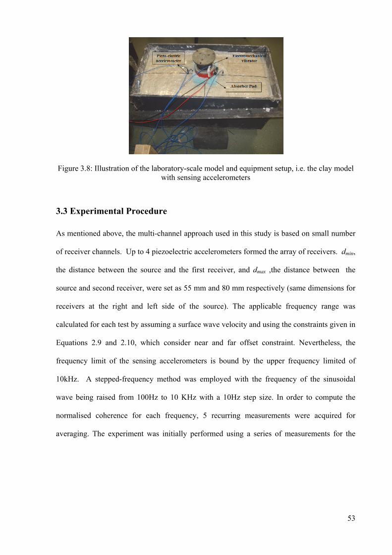
53
Figure 3.8: Illustration of the laboratory-scale model and equipment setup, i.e. the clay model with sensing accelerometers
3.3 Experimental Procedure
As mentioned above, the multi-channel approach used in this study is based on small number
of receiver channels. Up to 4 piezoelectric accelerometers formed the array of receivers. dmin,
the distance between the source and the first receiver, and dmax ,the distance between the
source and second receiver, were set as 55 mm and 80 mm respectively (same dimensions for
receivers at the right and left side of the source). The applicable frequency range was
calculated for each test by assuming a surface wave velocity and using the constraints given in
Equations 2.9 and 2.10, which consider near and far offset constraint. Nevertheless, the
frequency limit of the sensing accelerometers is bound by the upper frequency limited of
10kHz. A stepped-frequency method was employed with the frequency of the sinusoidal
wave being raised from 100Hz to 10 KHz with a 10Hz step size. In order to compute the
normalised coherence for each frequency, 5 recurring measurements were acquired for
averaging. The experiment was initially performed using a series of measurements for the
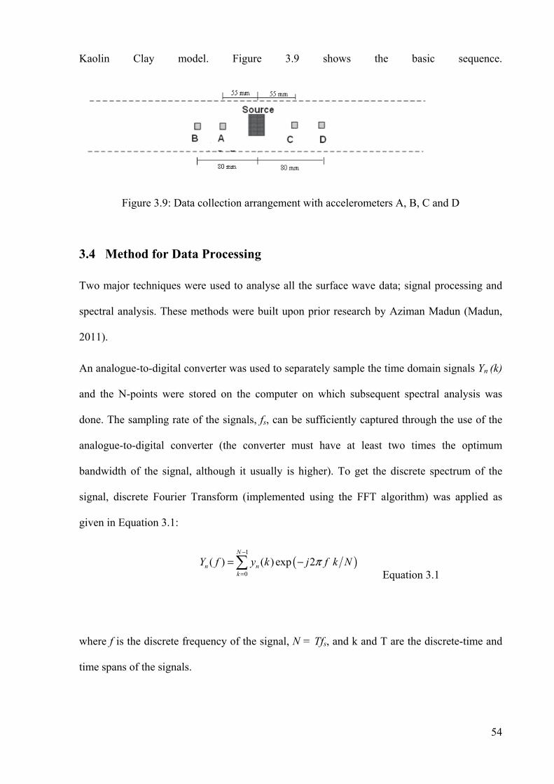
54
Kaolin Clay model. Figure 3.9 shows the basic sequence.
Figure 3.9: Data collection arrangement with accelerometers A, B, C and D
3.4 Method for Data Processing
Two major techniques were used to analyse all the surface wave data; signal processing and
spectral analysis. These methods were built upon prior research by Aziman Madun (Madun,
2011).
An analogue-to-digital converter was used to separately sample the time domain signals Yn (k)
and the N-points were stored on the computer on which subsequent spectral analysis was
done. The sampling rate of the signals, fs, can be sufficiently captured through the use of the
analogue-to-digital converter (the converter must have at least two times the optimum
bandwidth of the signal, although it usually is higher). To get the discrete spectrum of the
signal, discrete Fourier Transform (implemented using the FFT algorithm) was applied as
given in Equation 3.1:
( )
1
0
( ) ( ) exp 2N
n nk
Y f y k j f k Nπ−
=
= − Equation 3.1
where f is the discrete frequency of the signal, N = Tfs, and k and T are the discrete-time and
time spans of the signals.
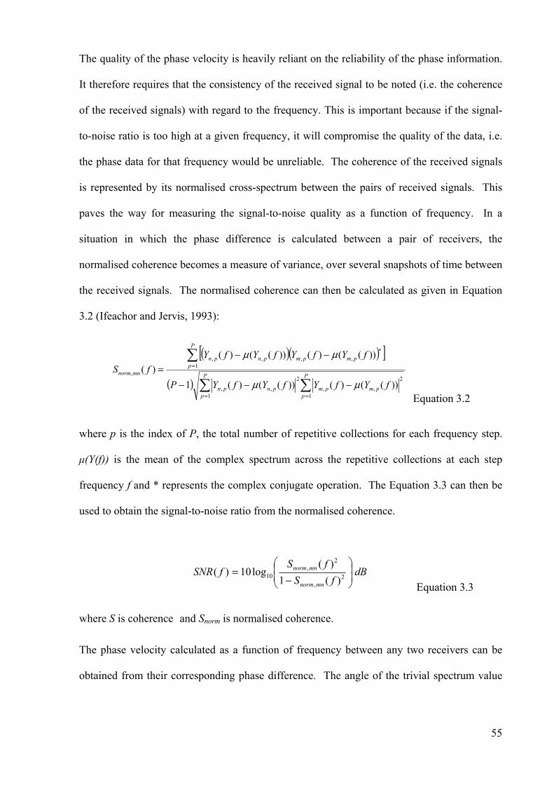
55
The quality of the phase velocity is heavily reliant on the reliability of the phase information.
It therefore requires that the consistency of the received signal to be noted (i.e. the coherence
of the received signals) with regard to the frequency. This is important because if the signal-
to-noise ratio is too high at a given frequency, it will compromise the quality of the data, i.e.
the phase data for that frequency would be unreliable. The coherence of the received signals
is represented by its normalised cross-spectrum between the pairs of received signals. This
paves the way for measuring the signal-to-noise quality as a function of frequency. In a
situation in which the phase difference is calculated between a pair of receivers, the
normalised coherence becomes a measure of variance, over several snapshots of time between
the received signals. The normalised coherence can then be calculated as given in Equation
3.2 (Ifeachor and Jervis, 1993):
( )( )[ ]
( )
= =
=
−−−
−−=
P
p
P
ppmpmpnpn
P
ppmpmpnpn
mnnorm
fYfYfYfYP
fYfYfYfYfS
1 1
2
,,
2
,,
1
*,,,,
,
))(()())(()(1
))(()())(()(
)(
μμ
μμ
Equation 3.2
where p is the index of P, the total number of repetitive collections for each frequency step.
μ(Y(f)) is the mean of the complex spectrum across the repetitive collections at each step
frequency f and * represents the complex conjugate operation. The Equation 3.3 can then be
used to obtain the signal-to-noise ratio from the normalised coherence.
dB
fSfS
fSNRmnnorm
mnnorm
−=
2,
2,
10 )(1
)(log10)(
Equation 3.3
where S is coherence and Snorm is normalised coherence.
The phase velocity calculated as a function of frequency between any two receivers can be
obtained from their corresponding phase difference. The angle of the trivial spectrum value
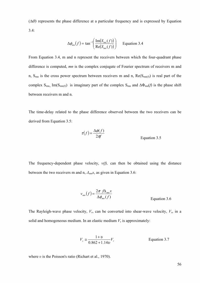
56
(Ư) represents the phase difference at a particular frequency and is expressed by Equation
3.4:
( ) ( )( )
=Δ −
)(Re
)(Imtan 1
fSfSf
mn
mnmnφ Equation 3.4
From Equation 3.4, m and n represent the receivers between which the four-quadrant phase
difference is computed, mn is the complex conjugate of Fourier spectrum of receivers m and
n, Smn is the cross power spectrum between receivers m and n, Re(Smn(f)) is real part of the
complex Smn,, Im(Smn(f)) is imaginary part of the complex Smn and ΔΦmn(f) is the phase shift
between receivers m and n.
The time-delay related to the phase difference observed between the two receivers can be
derived from Equation 3.5:
( )
fff
πφτ2
)(Δ= Equation 3.5
The frequency-dependent phase velocity, v(f), can then be obtained using the distance
between the two receivers m and n, Δmnx, as given in Equation 3.6:
( )
)(
2
fxffv
mn
mnmn φ
πΔ
Δ=
Equation 3.6
The Rayleigh-wave phase velocity, Vr, can be converted into shear-wave velocity, Vs, in a
solid and homogeneous medium. In an elastic medium Vs is approximately:
rs VVυ
υ14.1862.0
1
++≅ Equation 3.7
where υ is the Poisson's ratio (Richart et al., 1970).
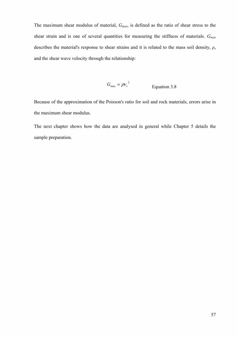
57
The maximum shear modulus of material, Gmax, is defined as the ratio of shear stress to the
shear strain and is one of several quantities for measuring the stiffness of materials. Gmax
describes the material's response to shear strains and it is related to the mass soil density, ρ,
and the shear wave velocity through the relationship:
2
max svG ρ= Equation 3.8
Because of the approximation of the Poisson's ratio for soil and rock materials, errors arise in
the maximum shear modulus.
The next chapter shows how the data are analysed in general while Chapter 5 details the
sample preparation.

59
Chapter 4
SUMMARY OF THE DESIGNED TEST PROCEDURE
4.1 Introduction
This chapter summarises the designed test procedure, while the test process and analysis of
results will be described in the subsequent chapters. The data analysis presented in this
chapter is in accordance with Madun (2010, 2011), who demonstrated the validity of the
methodology. The outcomes from the tests can be used to develop the surface wave test
method on models of natural soil for future work.
4.2 Data Processing
Each comprehensive set of measurements contains received signals from the 4 sensing
channels with the frequency range of 100 Hz to 10 kHz with a step-size of 10 Hz. The
collected data were processed after each session by using the Matlab software. Applying a
Fast Fourier Transform (FFT) to all the data, to acquire spectral representation of the received
signals, was the initial step in the process. The magnitude and angle from the complex results
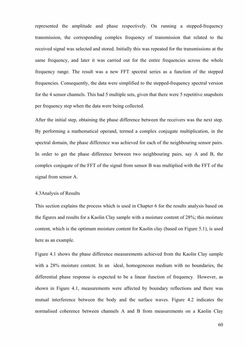
60
represented the amplitude and phase respectively. On running a stepped-frequency
transmission, the corresponding complex frequency of transmission that related to the
received signal was selected and stored. Initially this was repeated for the transmissions at the
same frequency, and later it was carried out for the entire frequencies across the whole
frequency range. The result was a new FFT spectral series as a function of the stepped
frequencies. Consequently, the data were simplified to the stepped-frequency spectral version
for the 4 sensor channels. This had 5 multiple sets, given that there were 5 repetitive snapshots
per frequency step when the data were being collected.
After the initial step, obtaining the phase difference between the receivers was the next step.
By performing a mathematical operand, termed a complex conjugate multiplication, in the
spectral domain, the phase difference was achieved for each of the neighbouring sensor pairs.
In order to get the phase difference between two neighbouring pairs, say A and B, the
complex conjugate of the FFT of the signal from sensor B was multiplied with the FFT of the
signal from sensor A.
4.3Analysis of Results
This section explains the process which is used in Chapter 6 for the results analysis based on
the figures and results for a Kaolin Clay sample with a moisture content of 28%; this moisture
content, which is the optimum moisture content for Kaolin clay (based on Figure 5.1), is used
here as an example.
Figure 4.1 shows the phase difference measurements achieved from the Kaolin Clay sample
with a 28% moisture content. In an ideal, homogeneous medium with no boundaries, the
differential phase response is expected to be a linear function of frequency. However, as
shown in Figure 4.1, measurements were affected by boundary reflections and there was
mutual interference between the body and the surface waves. Figure 4.2 indicates the
normalised coherence between channels A and B from measurements on a Kaolin Clay
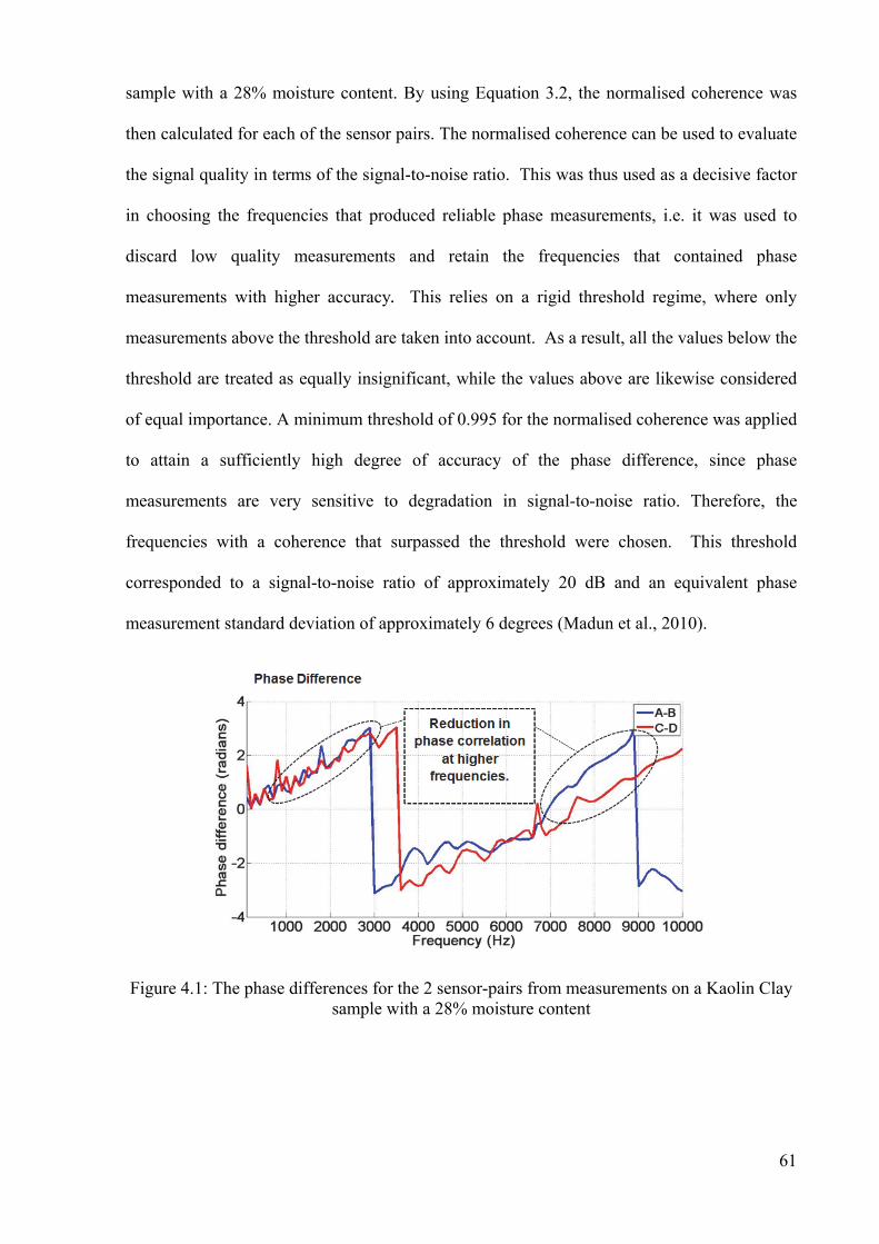
61
sample with a 28% moisture content. By using Equation 3.2, the normalised coherence was
then calculated for each of the sensor pairs. The normalised coherence can be used to evaluate
the signal quality in terms of the signal-to-noise ratio. This was thus used as a decisive factor
in choosing the frequencies that produced reliable phase measurements, i.e. it was used to
discard low quality measurements and retain the frequencies that contained phase
measurements with higher accuracy. This relies on a rigid threshold regime, where only
measurements above the threshold are taken into account. As a result, all the values below the
threshold are treated as equally insignificant, while the values above are likewise considered
of equal importance. A minimum threshold of 0.995 for the normalised coherence was applied
to attain a sufficiently high degree of accuracy of the phase difference, since phase
measurements are very sensitive to degradation in signal-to-noise ratio. Therefore, the
frequencies with a coherence that surpassed the threshold were chosen. This threshold
corresponded to a signal-to-noise ratio of approximately 20 dB and an equivalent phase
measurement standard deviation of approximately 6 degrees (Madun et al., 2010).
Figure 4.1: The phase differences for the 2 sensor-pairs from measurements on a Kaolin Clay sample with a 28% moisture content
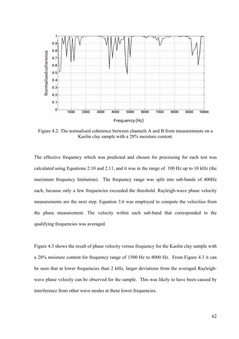
62
Figure 4.2: The normalised coherence between channels A and B from measurements on a Kaolin clay sample with a 28% moisture content.
The effective frequency which was predicted and chosen for processing for each test was
calculated using Equations 2.10 and 2.11, and it was in the range of 100 Hz up to 10 kHz (the
maximum frequency limitation). The frequency range was split into sub-bands of 400Hz
each, because only a few frequencies exceeded the threshold. Rayleigh-wave phase velocity
measurements are the next step. Equation 3.6 was employed to compute the velocities from
the phase measurement. The velocity within each sub-band that corresponded to the
qualifying frequencies was averaged.
Figure 4.3 shows the result of phase velocity versus frequency for the Kaolin clay sample with
a 28% moisture content for frequency range of 1500 Hz to 8000 Hz. From Figure 4.3 it can
be seen that at lower frequencies than 2 kHz, larger deviations from the averaged Rayleigh-
wave phase velocity can be observed for the sample. This was likely to have been caused by
interference from other wave modes at these lower frequencies.

63
Figure 4.3: Phase velocity versus frequency for the Kaolin clay sample with a 28% moisture content
The Rayleigh-wave phase velocities were converted into shear-wave velocities by a factor of
1.08, based upon the adoption of a Poisson’s ratio of 0.3 in Equation 3.7. In the situation
where more discrete samples are obtainable either through the use of a wider frequency range,
or in situations where there are more frequencies that contain precise phase measurements, the
shear-wave velocity values can be interpolated to get a smoothed dataset. The relationship
between the shear wave velocity and the moisture content of the soil will be investigated, so
this will show how soil properties such as moisture content and density influence acoustic
wave transmission. This will allow the formulation of a correlation between acoustic and
geotechnical properties.

64
Chapter 5
DETAILED PROGRAMME OF WORK
5.1 Introduction
This chapter gives a summary of the experiments conducted to measure the shear wave
velocity for the samples with different moisture content. The experimental models are
constructed based on the aim of this study, which is to assess how soil properties influence
acoustic wave transmission and how the results can be used to develop a correlation between
acoustic and geotechnical properties. The programme involved 8 tests using a plastic box
filled with Kaolin Clay or Oxford Clay, each using 4 different moisture contents.
5.2 Clay Materials Used in Test Beds
In this research, the Clay test beds were made of compacted Oxford Clay and Kaolin Clay
with different moisture contents. Kaolin Clay mixed from dry, processed powdered Clay was
used initially. This reduced the level of variation in the course of the test programme and also
ensured a high level of sample control. A single batch of Oxford Clay was obtained from the
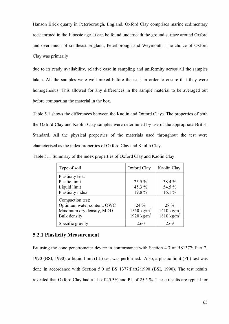
65
Hanson Brick quarry in Peterborough, England. Oxford Clay comprises marine sedimentary
rock formed in the Jurassic age. It can be found underneath the ground surface around Oxford
and over much of southeast England, Peterborough and Weymouth. The choice of Oxford
Clay was primarily
due to its ready availability, relative ease in sampling and uniformity across all the samples
taken. All the samples were well mixed before the tests in order to ensure that they were
homogeneous. This allowed for any differences in the sample material to be averaged out
before compacting the material in the box.
Table 5.1 shows the differences between the Kaolin and Oxford Clays. The properties of both
the Oxford Clay and Kaolin Clay samples were determined by use of the appropriate British
Standard. All the physical properties of the materials used throughout the test were
characterised as the index properties of Oxford Clay and Kaolin Clay.
Table 5.1: Summary of the index properties of Oxford Clay and Kaolin Clay
Type of soil Oxford Clay Kaolin Clay
Plasticity test: Plastic limit Liquid limit Plasticity index
25.5 % 45.3 % 19.8 %
38.4 % 54.5 % 16.1 %
Compaction test: Optimum water content, OWC Maximum dry density, MDD Bulk density
24 %
1550 kg/m3 1920 kg/m3
28 %
1410 kg/m3 1810 kg/m3
Specific gravity 2.60 2.69
5.2.1 Plasticity Measurement
By using the cone penetrometer device in conformance with Section 4.3 of BS1377: Part 2:
1990 (BSI, 1990), a liquid limit (LL) test was performed. Also, a plastic limit (PL) test was
done in accordance with Section 5.0 of BS 1377:Part2:1990 (BSI, 1990). The test results
revealed that Oxford Clay had a LL of 45.3% and PL of 25.5 %. These results are typical for
66
Oxford Clay as proposed by Lee (2001). In contrast, Kaolin Clay had a LL of 54.5% and PL
of 38.4%, which agrees with the standard values reported by John (2011).
5.2.2 Specific Gravity
Using the small pyknometer method in accordance with Section 8.3 of BS 1377: Part 2:1990
(BSI, 1990), specific gravity tests were carried out. The soil used for testing was oven-dried
soil which passed through a 2mm sieve. The precise specific gravity of the Oxford Clay was
2.60 and for Kaolin Clay was 2.69, which is also in line with accepted values for these soil
types.
5.2.3 Compaction Test
The Clay compaction tests were conducted based on BS 1377: Part 4.7: 1990 (BSI, 1990),
using the 2.5 kg hammer method. This technique makes use of a 2.5 kg hand compaction
hammer and a compaction mould measuring one litre. This method is often referred to as the
'Proctor' test. A dry density-moisture content relationship for Oxford Clay and Kaolin Clay is
shown in Figure 5.1. The Oxford Clay and Kaolin Clay have a highest dry density of
approximately 1550 kg/m3 and 1410 kg/m3 at optimum water contents of 24% and 28%
respectively.
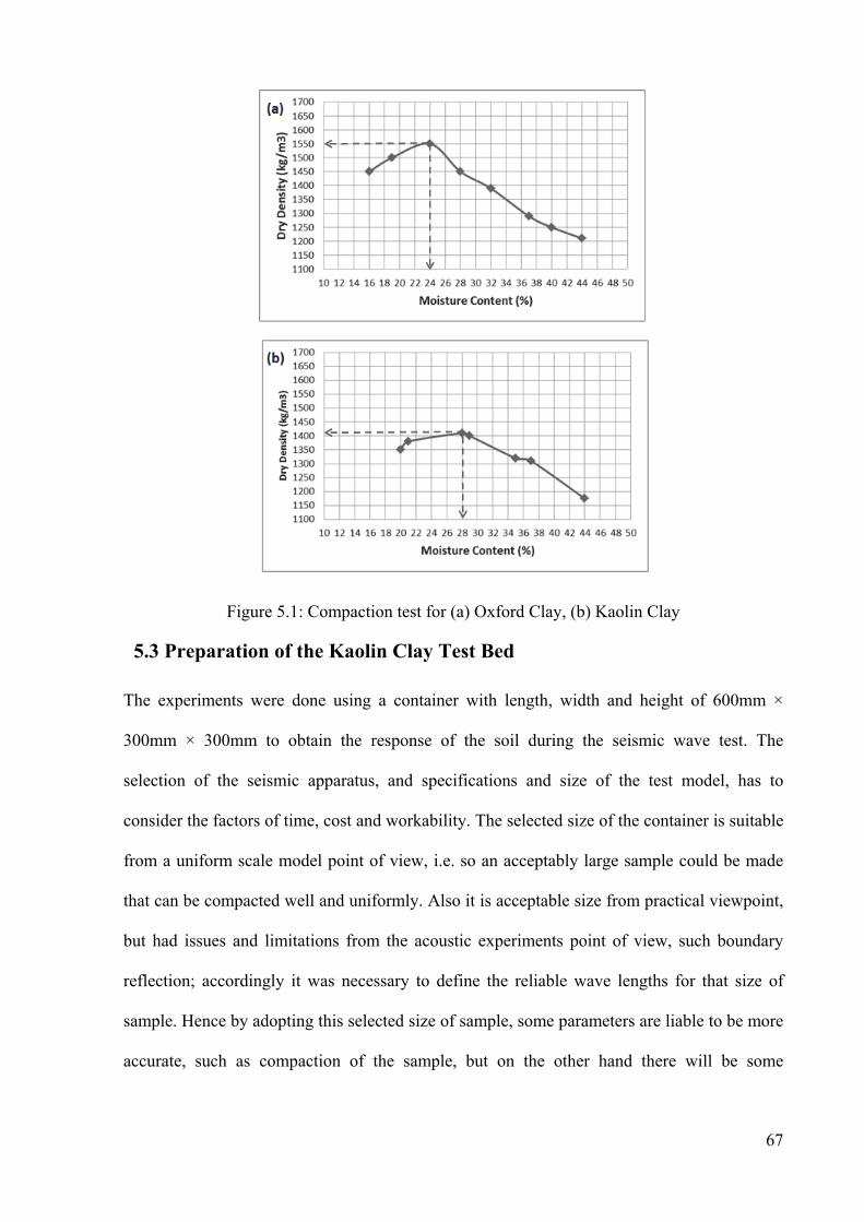
67
Figure 5.1: Compaction test for (a) Oxford Clay, (b) Kaolin Clay
5.3 Preparation of the Kaolin Clay Test Bed
The experiments were done using a container with length, width and height of 600mm ×
300mm × 300mm to obtain the response of the soil during the seismic wave test. The
selection of the seismic apparatus, and specifications and size of the test model, has to
consider the factors of time, cost and workability. The selected size of the container is suitable
from a uniform scale model point of view, i.e. so an acceptably large sample could be made
that can be compacted well and uniformly. Also it is acceptable size from practical viewpoint,
but had issues and limitations from the acoustic experiments point of view, such boundary
reflection; accordingly it was necessary to define the reliable wave lengths for that size of
sample. Hence by adopting this selected size of sample, some parameters are liable to be more
accurate, such as compaction of the sample, but on the other hand there will be some

68
limitation such as reliable wavelength, because of the boundary reflections. The chosen
dimensions were therefore considered to be an acceptable compromise.
The test results were used to understand the response of the soil due to wave transmission and
also to identify the phase velocity of the Clay. Based on the index properties of the Kaolin
Clay (Table 5.1), four different samples of dry Kaolin was repeatedly mixed with water to
achieve three different levels of moisture content: 24% (significantly below the OWC), 28%
(the OWC), 33% (significantly above the OWC), and a repeat test at 28%. The 3 different
moisture contents were considered to provide a good range of moisture content for the test
results. To prove the repeatability of the test procedure, one of these 3 moisture content (the
OWC) was chosen for repeat testing. Weights of 75kg, 76kg, 80kg and 75 kg of Kaolin were
mixed using 18.0kg, 21.3kg, 26.4kg and 21.0kg of water respectively. Each Kaolin sample
was mixed with water using a large mixer for half an hour. After pouring the mixture to
achieve successive layers of 50mm thickness into the plastic box, each layer was then
compacted using a vibrator. Every 100mm, three standard thin-walled tubes were used to
collect samples from each compacted layer to measure the density of the layer to make sure
that all parts of the sample had the same density. These tubes were knocked into the
compacted layer surface at three different points, and then the size and weight of the three
cylindrical soil samples were measured to calculate the density. The process is shown in
Figure 5.2 and the results are indicated in Table 5.2. It was not possible to refill the holes with
the same sample as the samples needed to be placed in the oven to calculate the moisture
content, needed to obtain the density. So the same mixture was used to fill the holes and
compacted by using the vibrator at the same time with the same energy; in this way the
replaced material was considered to have the same density to a good approximation. This
process continued until the final layer was constructed. In order to ensure good contact for the
next Clay filled layer, the Clay surface was grooved to avoid a plane of weakness between the
layers (i.e. stratification).

69
Figure 5.2: (a) Mixed Kaolin Clay ready to be compacted with a vibrator, (b) wooden plates used to smooth the surface of Clay layer, (c) tubes in place to retrieve samples for density
testing, and (d) final Kaolin Clay bed test
Table 5.2: Results for the density measurement for each layer during the preparation of the Kaolin Clay test bed for different moisture contents
Clay type
Moisture content %
Compounds Layers Density
(kg/m3)
Averaged density of each layer
Bulk density, kg/m³
Dry density, kg/m³
Kaolin Clay
24% Clay: 75 kg
Water: 18.0 kg
1 1365
1359 1750
1380
2 1360
3 1352
28% Clay: 76 kg
Water: 21.3 kg
1 1498
1495 2260 1410 2 1502
3 1485
33% Clay: 80 kg
Water: 26.4 kg
1 1506
1488 2110 1340 2 1480
3 1478
28% Clay: 75 kg
Water: 21.0 kg
1 1472
1446 2260 1410 2 1430
3 1438
5.4 Preparation of the Oxford Clay Test Bed
The index properties of the Oxford Clay are given in Table 5.1. Oxford Clay and water were
repeatedly mixed to obtain different moisture contents of: 19%, 24%, 32% and a repeat test at
32%, again to provide a spread significantly above and below the OWC and to provide a

70
sample to test for repeatability. Oxford Clay with weights of 79.1kg, 83.7kg, 80.0kg and
73.0kg was mixed using 15.2kg, 20.0kg, 24.0kg and 23.4kg of water respectively. For each
Oxford Clay-water mixture, a process similar to that using Kaolin Clay was carried out.
Results for the density measurement for each layer during the preparation of the Oxford Clay
Test bed are shown in Table 5.3. Figure 5.3 shows the compaction and density measurement
procedures for the Oxford Clay test bed.
Figure 5.3: (a) Compacting Oxford Clay with a vibrator, (b) wooden plates used to smooth the surface of Clay layer, (c) and (d) thin walled tubes used to collect sample to measure the
density of the Clay layer.
Table 5.3: Results for the density measurement for each layer during the preparation of the Oxford Clay Test bed for different moisture contents
Clay type
Moisture content %
Compounds Layers Density
(kg/m3)
Averaged density of each layer
Bulk density, kg/m³
Dry density, kg/m³
Oxford Clay
19% Clay: 79.1 kg
Water: 15.2 kg
1 1380
1423 1870 1500 2 1402
3 1488
24% Clay: 83.7 kg
Water: 20.0 kg
1 1602 1606 1820 1550
2 1620
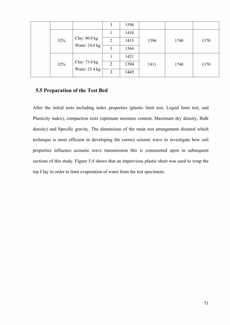
71
3 1598
32% Clay: 80.0 kg
Water: 24.0 kg
1 1410
1396 1740 1370 2 1415
3 1364
32% Clay: 73.0 kg
Water: 23.4 kg
1 1421
1411 1740 1370 2 1394
3 1445
5.5 Preparation of the Test Bed
After the initial tests including index properties (plastic limit test, Liquid limit test, and
Plasticity index), compaction tests (optimum moisture content, Maximum dry density, Bulk
density) and Specific gravity. The dimensions of the main test arrangement dictated which
technique is most efficient in developing the correct seismic wave to investigate how soil
properties influence acoustic wave transmission this is commented upon in subsequent
sections of this study. Figure 5.4 shows that an impervious plastic sheet was used to wrap the
top Clay in order to limit evaporation of water from the test specimens.
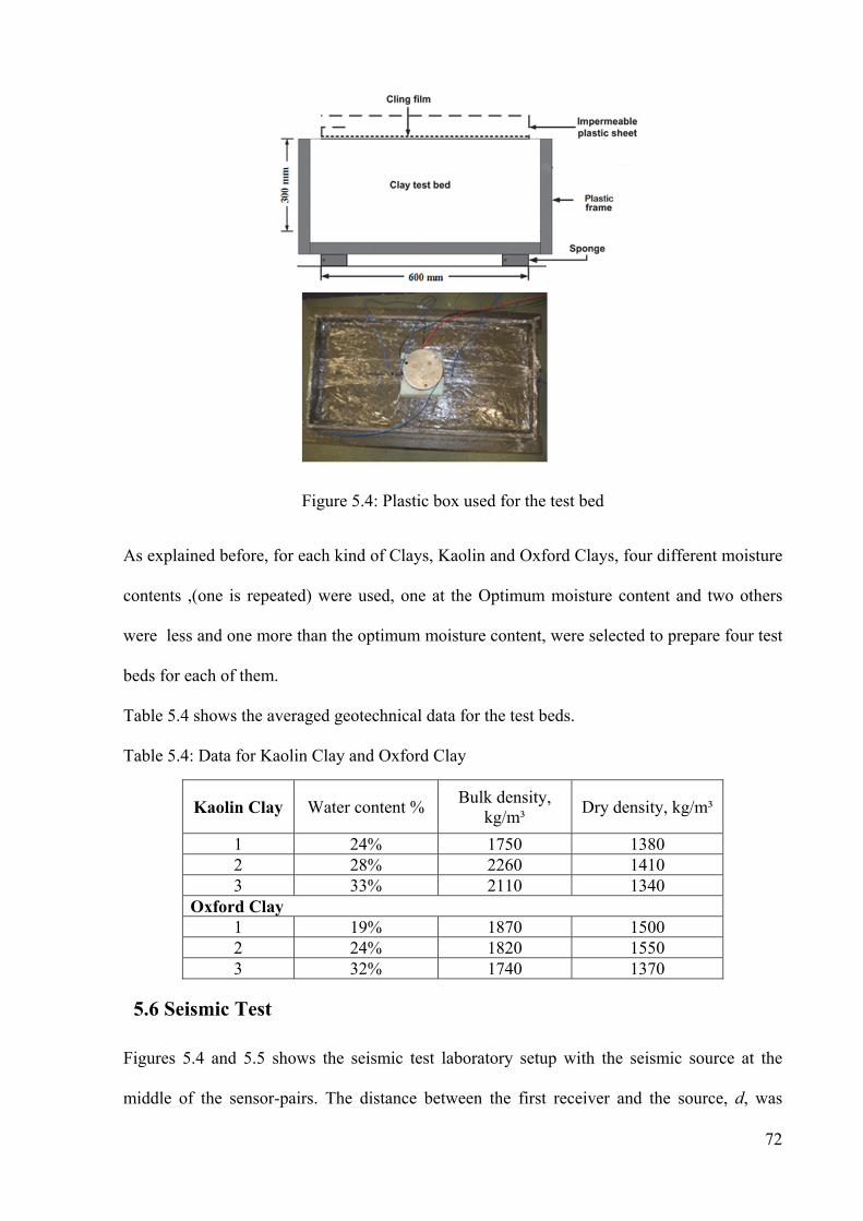
72
Figure 5.4: Plastic box used for the test bed
As explained before, for each kind of Clays, Kaolin and Oxford Clays, four different moisture
contents ,(one is repeated) were used, one at the Optimum moisture content and two others
were less and one more than the optimum moisture content, were selected to prepare four test
beds for each of them.
Table 5.4 shows the averaged geotechnical data for the test beds.
Table 5.4: Data for Kaolin Clay and Oxford Clay
Kaolin Clay Water content % Bulk density,
kg/m³ Dry density, kg/m³
1 24% 1750 1380 2 28% 2260 1410 3 33% 2110 1340
Oxford Clay 1 19% 1870 1500 2 24% 1820 1550 3 32% 1740 1370
5.6 Seismic Test
Figures 5.4 and 5.5 shows the seismic test laboratory setup with the seismic source at the
middle of the sensor-pairs. The distance between the first receiver and the source, d, was
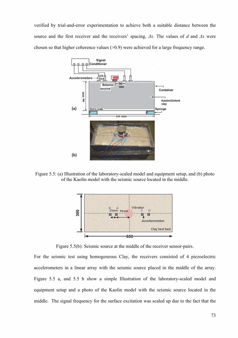
73
verified by trial-and-error experimentation to achieve both a suitable distance between the
source and the first receiver and the receivers’ spacing, Δx. The values of d and Δx were
chosen so that higher coherence values (>0.9) were achieved for a large frequency range.
Figure 5.5: (a) Illustration of the laboratory-scaled model and equipment setup, and (b) photo of the Kaolin model with the seismic source located in the middle.
Figure 5.5(b): Seismic source at the middle of the receiver sensor-pairs.
For the seismic test using homogeneous Clay, the receivers consisted of 4 piezoelectric
accelerometers in a linear array with the seismic source placed in the middle of the array.
Figure 5.5 a, and 5.5 b show a simple Illustration of the laboratory-scaled model and
equipment setup and a photo of the Kaolin model with the seismic source located in the
middle. The signal frequency for the surface excitation was scaled up due to the fact that the
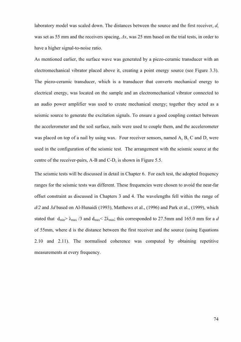
74
laboratory model was scaled down. The distances between the source and the first receiver, d,
was set as 55 mm and the receivers spacing, Δx, was 25 mm based on the trial tests, in order to
have a higher signal-to-noise ratio.
As mentioned earlier, the surface wave was generated by a piezo-ceramic transducer with an
electromechanical vibrator placed above it, creating a point energy source (see Figure 3.3).
The piezo-ceramic transducer, which is a transducer that converts mechanical energy to
electrical energy, was located on the sample and an electromechanical vibrator connected to
an audio power amplifier was used to create mechanical energy; together they acted as a
seismic source to generate the excitation signals. To ensure a good coupling contact between
the accelerometer and the soil surface, nails were used to couple them, and the accelerometer
was placed on top of a nail by using wax. Four receiver sensors, named A, B, C and D, were
used in the configuration of the seismic test. The arrangement with the seismic source at the
centre of the receiver-pairs, A-B and C-D, is shown in Figure 5.5.
The seismic tests will be discussed in detail in Chapter 6. For each test, the adopted frequency
ranges for the seismic tests was different. These frequencies were chosen to avoid the near-far
offset constraint as discussed in Chapters 3 and 4. The wavelengths fell within the range of
d/2 and 3d based on Al-Hunaidi (1993), Matthews et al., (1996) and Park et al., (1999), which
stated that dmin> λmax /3 and dmax< 2λmin; this corresponded to 27.5mm and 165.0 mm for a d
of 55mm, where d is the distance between the first receiver and the source (using Equations
2.10 and 2.11). The normalised coherence was computed by obtaining repetitive
measurements at every frequency.

76
Chapter 6
ANALYSIS
6.1 Introduction
In this chapter, the results of the experimental work are presented, analysed and discussed.
Kaolin clay and Oxford Clay were used to develop the test bed and detailed test results of
phase velocity measurements in a physical model of homogeneous Kaolin clay and Oxford
Clay have been analysed.
6.2 Kaolin clay – 28% Moisture Content
A linear array of accelerometers consisting of 4 sensors and a seismic source at the middle of
the array was used for testing of the Kaolin clay physical model. The excitation was initially
done with a frequency range of 100Hz to 10,000Hz, using a stepped-frequency approach with
a step-size of 100Hz. At each frequency step, a set of tests with a total of 5 snapshot
measurements was obtained, both for averaging and to calculate the normalised coherence.
The signal quality in terms of the signal-to-noise ratio showed a degradation when the
frequency was less than 1500Hz, when it was between 4000Hz and 5000Hz and when it
reached 9000 Hz. This is illustrated in Figure 6.1. Based on the results from Figure 6.1 and
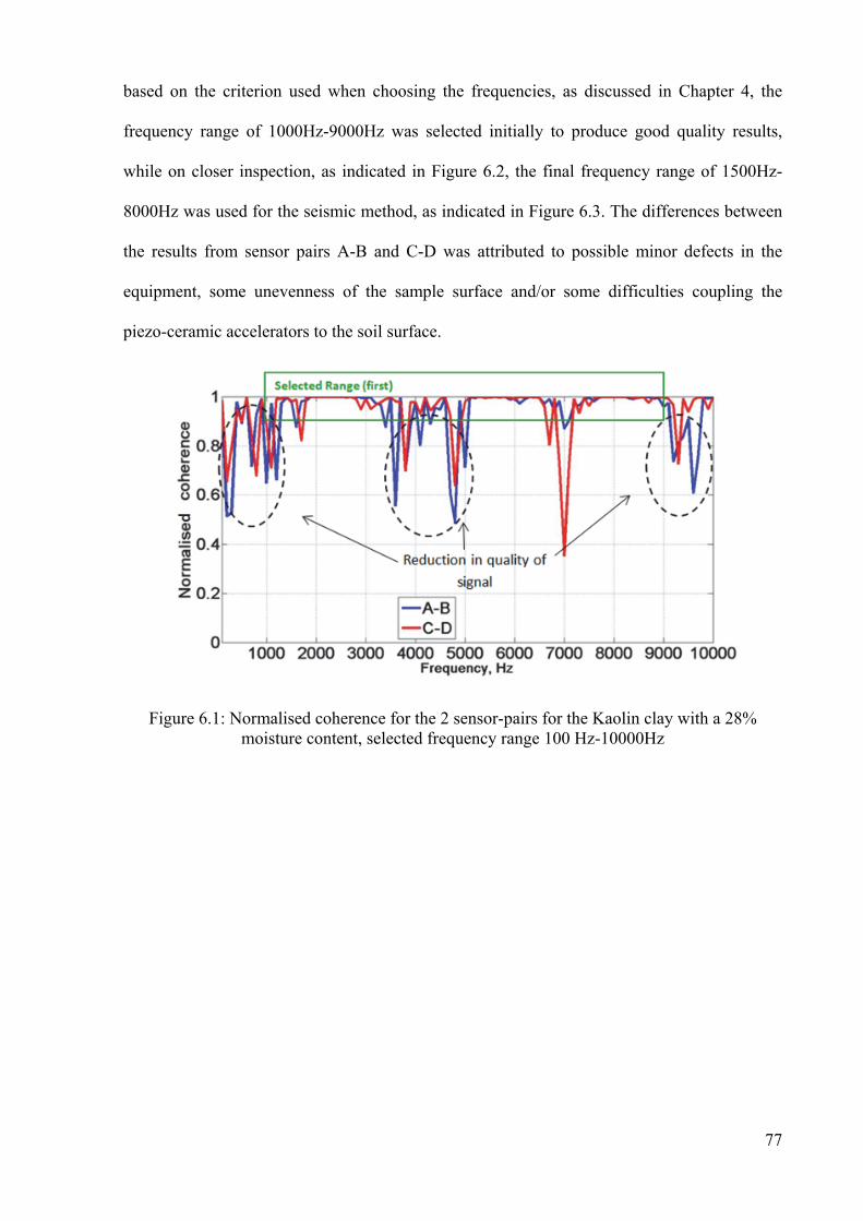
77
based on the criterion used when choosing the frequencies, as discussed in Chapter 4, the
frequency range of 1000Hz-9000Hz was selected initially to produce good quality results,
while on closer inspection, as indicated in Figure 6.2, the final frequency range of 1500Hz-
8000Hz was used for the seismic method, as indicated in Figure 6.3. The differences between
the results from sensor pairs A-B and C-D was attributed to possible minor defects in the
equipment, some unevenness of the sample surface and/or some difficulties coupling the
piezo-ceramic accelerators to the soil surface.
Figure 6.1: Normalised coherence for the 2 sensor-pairs for the Kaolin clay with a 28% moisture content, selected frequency range 100 Hz-10000Hz
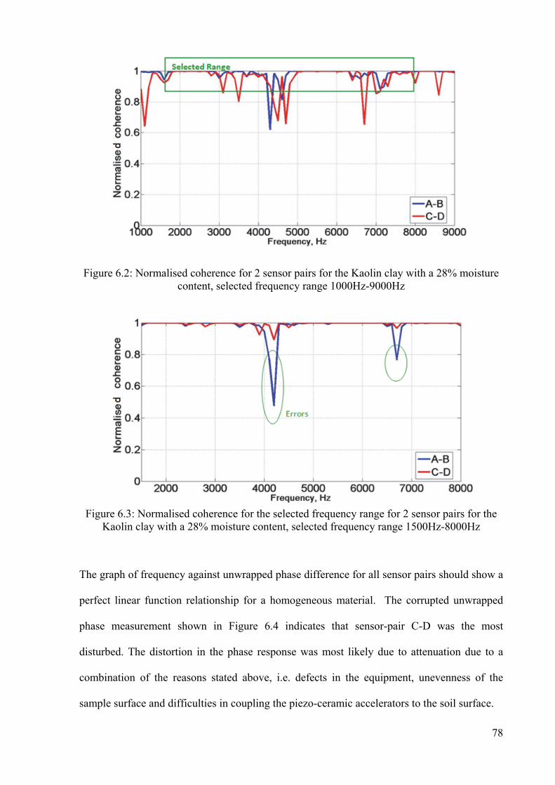
78
Figure 6.2: Normalised coherence for 2 sensor pairs for the Kaolin clay with a 28% moisture content, selected frequency range 1000Hz-9000Hz
Figure 6.3: Normalised coherence for the selected frequency range for 2 sensor pairs for the
Kaolin clay with a 28% moisture content, selected frequency range 1500Hz-8000Hz
The graph of frequency against unwrapped phase difference for all sensor pairs should show a
perfect linear function relationship for a homogeneous material. The corrupted unwrapped
phase measurement shown in Figure 6.4 indicates that sensor-pair C-D was the most
disturbed. The distortion in the phase response was most likely due to attenuation due to a
combination of the reasons stated above, i.e. defects in the equipment, unevenness of the
sample surface and difficulties in coupling the piezo-ceramic accelerators to the soil surface.

79
Figure 6.4: Unwrapped phase differences against frequency showing an almost linear function for the sensor pairs A-B and C-D for Kaolin clay with a 28% moisture content and a
frequency range of 1500 Hz-8000Hz
The phase velocity was calculated for each frequency from the phase difference and the
distance between the sensors (using Equation 3.6). The graph of the frequency versus phase
velocity is shown in Figure 6.5, which indicates that the phase velocity range for the
frequency range of 1500Hz-8000Hz is approximately 140 m/s to 250m/s for the Kaolin clay
with a 28% moisture content.

80
Figure 6.5: Phase velocity versus frequency showing the dispersive curve for Kaolin clay with a 28% moisture content and a frequency range of 1500Hz-8000Hz
The variation of the phase velocity with wavelength is shown in Figure 6.6. It shows that
signals with small wavelengths, between 4 and 6 cm, tended to attenuate quicker, the majority
of results falling between 170-230m/s approximately, than signals with larger wavelengths,
between 6 cm and 16 cm, for which there are more results of phase velocity less than 170 m/s.
The phase velocities deviation was thought not to be caused by the change of clay properties,
but by the frequencies/wavelength constraint that influences the near- and far-offset distance
of the source from the receivers, as well as some reflected waves from the boundary of the
clay container (Madun, 2011).
This plot is important to evaluate the reliability of the phase velocity data, which in an ideal
situation should be constant across a wide range of wavelengths for homogeneous clay. It is
important to verify the reliability of the data not only on the basis of coherence threshold, but
also on acceptable (i.e. approximately constant) range of phase velocity with changes in
wavelengths.
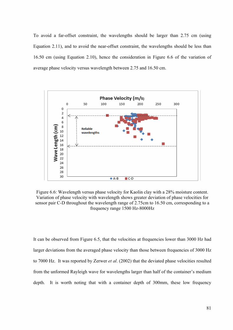
81
To avoid a far-offset constraint, the wavelengths should be larger than 2.75 cm (using
Equation 2.11), and to avoid the near-offset constraint, the wavelengths should be less than
16.50 cm (using Equation 2.10), hence the consideration in Figure 6.6 of the variation of
average phase velocity versus wavelength between 2.75 and 16.50 cm.
Figure 6.6: Wavelength versus phase velocity for Kaolin clay with a 28% moisture content. Variation of phase velocity with wavelength shows greater deviation of phase velocities for sensor pair C-D throughout the wavelength range of 2.75cm to 16.50 cm, corresponding to a
frequency range 1500 Hz-8000Hz
It can be observed from Figure 6.5, that the velocities at frequencies lower than 3000 Hz had
larger deviations from the averaged phase velocity than those between frequencies of 3000 Hz
to 7000 Hz. It was reported by Zerwer et al. (2002) that the deviated phase velocities resulted
from the unformed Rayleigh wave for wavelengths larger than half of the container’s medium
depth. It is worth noting that with a container depth of 300mm, these low frequency

82
distortions were likely to be caused by the small physical size of the clay container, in which
significant noise from the boundary and bottom reflections occurred.
The C-D sensor-pair shows larger phase velocity deviations compared with the A-B sensor
pair. This could be due to differences in the effectiveness with which these accelerometers
were coupled to the surface, while generally large deviation could be due to insufficient
energy exacerbated by interfering reflected waves from the boundary of the container. The
phase velocities across the frequencies were not totally non-dispersive, thus suggesting that
the Kaolin clay is not absolutely homogeneous due to experimental errors in the sample
preparation and compaction of the sample.
The useful frequency ranges can be based on using Equations 2.10 and 2.11, and limitation of
the maximum wavelength to half of the container depth. It is worth noting that the
expectation is that the phase velocity in soft clay is 200 m/s (McDowell et al., 2002, and
Parasnis, 1997).
6.2.1 Repeatability of the Tests - Kaolin clay
In order to test the repeatability of the experiments, a second test using Kaolin clay with a
moisture content of a 28% was carried out. For this, the test tank was emptied and a new batch
of clay was mixed, and placed and compacted in the test bed as described before. This test
was designed to demonstrate that the measurement system can give reliable results of phase
velocities and shear parameters (which are presented and discussed in Chapter 7). Figures 6.7
and 6.8 indicate the results for Kaolin clay with a 28% moisture content as a repeated test.
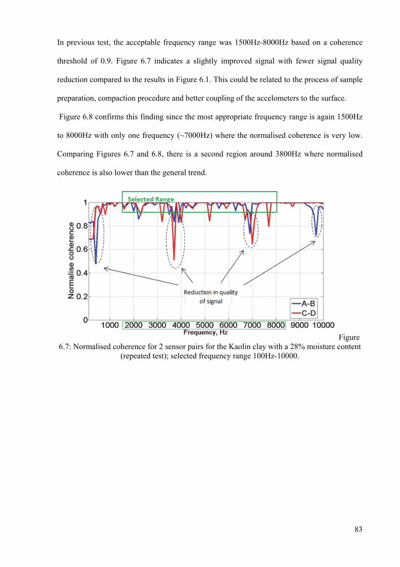
83
In previous test, the acceptable frequency range was 1500Hz-8000Hz based on a coherence
threshold of 0.9. Figure 6.7 indicates a slightly improved signal with fewer signal quality
reduction compared to the results in Figure 6.1. This could be related to the process of sample
preparation, compaction procedure and better coupling of the accelometers to the surface.
Figure 6.8 confirms this finding since the most appropriate frequency range is again 1500Hz
to 8000Hz with only one frequency (~7000Hz) where the normalised coherence is very low.
Comparing Figures 6.7 and 6.8, there is a second region around 3800Hz where normalised
coherence is also lower than the general trend.
Figure 6.7: Normalised coherence for 2 sensor pairs for the Kaolin clay with a 28% moisture content
(repeated test); selected frequency range 100Hz-10000.
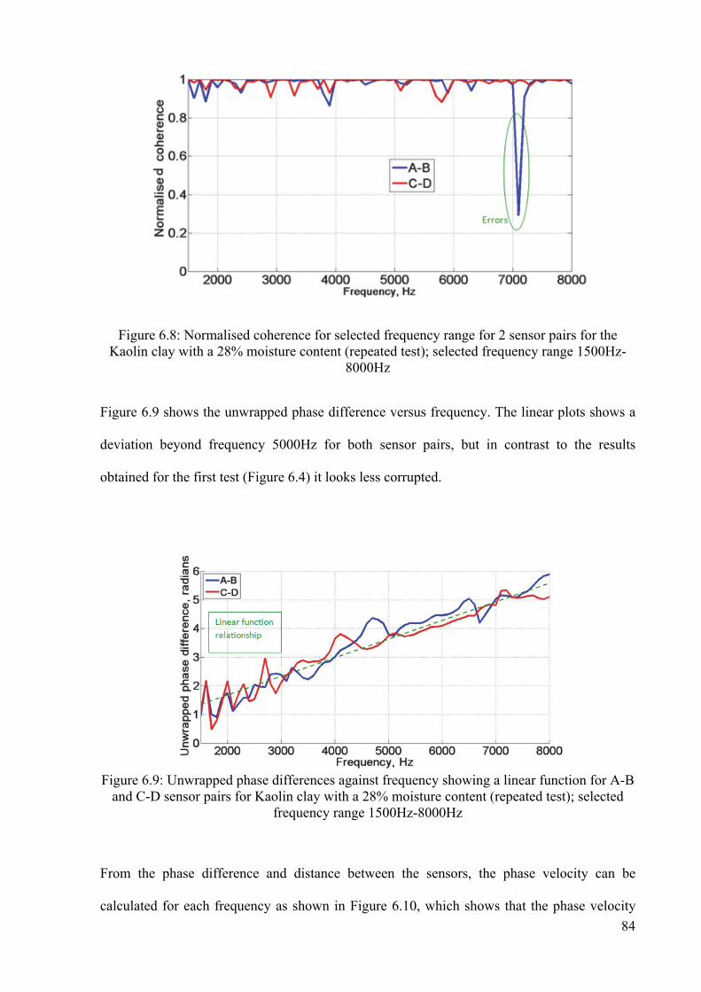
84
Figure 6.8: Normalised coherence for selected frequency range for 2 sensor pairs for the Kaolin clay with a 28% moisture content (repeated test); selected frequency range 1500Hz-
8000Hz
Figure 6.9 shows the unwrapped phase difference versus frequency. The linear plots shows a
deviation beyond frequency 5000Hz for both sensor pairs, but in contrast to the results
obtained for the first test (Figure 6.4) it looks less corrupted.
Figure 6.9: Unwrapped phase differences against frequency showing a linear function for A-B
and C-D sensor pairs for Kaolin clay with a 28% moisture content (repeated test); selected frequency range 1500Hz-8000Hz
From the phase difference and distance between the sensors, the phase velocity can be
calculated for each frequency as shown in Figure 6.10, which shows that the phase velocity

85
range for the frequency range of 1500Hz-8000Hz is approximately 120m/s to 230m/s for the
Kaolin clay with a 28% moisture content. As shown in Figure 6.11, this range of phase
velocity measurements is similar to the main test for Kaolin clay with a 28% moisture content.
Figure 6.12 shows the variation of the phase velocity with wavelength. For this test, the range
of reliable wavelength is slightly larger than for the first test. Nevertheless the differences are
small so that it can be assumed that the test is repeatable and the results reliable.
Figure 6.10: Phase velocity versus frequency showing the dispersive curve for the Kaolin clay with a 28% moisture content (repeated test); the frequency range was 1500Hz-8000Hz
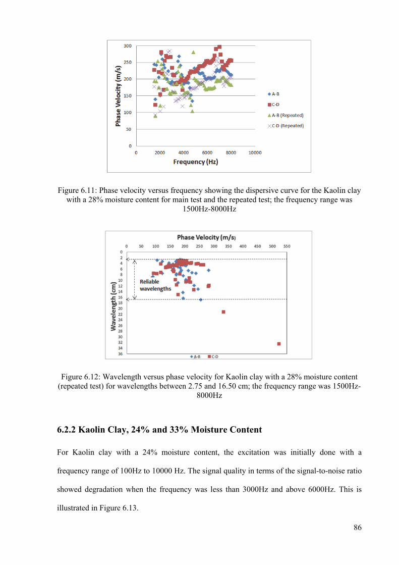
86
Figure 6.11: Phase velocity versus frequency showing the dispersive curve for the Kaolin clay with a 28% moisture content for main test and the repeated test; the frequency range was
1500Hz-8000Hz
Figure 6.12: Wavelength versus phase velocity for Kaolin clay with a 28% moisture content (repeated test) for wavelengths between 2.75 and 16.50 cm; the frequency range was 1500Hz-
8000Hz
6.2.2 Kaolin Clay, 24% and 33% Moisture Content
For Kaolin clay with a 24% moisture content, the excitation was initially done with a
frequency range of 100Hz to 10000 Hz. The signal quality in terms of the signal-to-noise ratio
showed degradation when the frequency was less than 3000Hz and above 6000Hz. This is
illustrated in Figure 6.13.
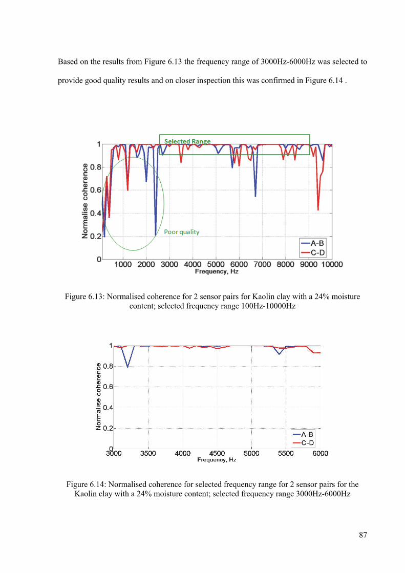
87
Based on the results from Figure 6.13 the frequency range of 3000Hz-6000Hz was selected to
provide good quality results and on closer inspection this was confirmed in Figure 6.14 .
Figure 6.13: Normalised coherence for 2 sensor pairs for Kaolin clay with a 24% moisture content; selected frequency range 100Hz-10000Hz
Figure 6.14: Normalised coherence for selected frequency range for 2 sensor pairs for the Kaolin clay with a 24% moisture content; selected frequency range 3000Hz-6000Hz

88
Figure 6.15 shows the unwrapped phase difference versus frequency. The linear plots show a
deviation beyond frequency 4000Hz and above 5000Hz for both sensor pairs.
Figure 6.15: Unwrapped phase differences show linear function for A-B and C-D sensor pairs for Kaolin clay with a 24% moisture content; the frequency range was 3000Hz-6000Hz
As explained previously the phase velocity can be calculated from the phase difference and
distance between the sensors, for each frequency. This is plotted in Figure 6.16, which shows
that the phase velocity range for the frequency range of 3000Hz-6000Hz is approximately
200m/s to 300m/s for the Kaolin clay with a 24% moisture content. This is larger than the
phase velocity range for Kaolin clay with a 28% moisture content.

89
Figure 6.16: Phase velocity versus frequency showing dispersive curve for the Kaolin clay
with a 24% moisture content; the frequency range was 3000Hz-6000Hz
Figure 6.17 shows the variation of the phase velocity with wavelength for the Kaolin clay
with a 24% moisture content.
Figure 6.17: Wavelength versus phase velocity for Kaolin clay with a 24% moisture content
for wavelengths between 2.75 and 16.50 cm; the frequency range was 3000Hz-6000Hz
For Kaolin clay with a 33% moisture content, the excitation was initially done with a
frequency range of 100Hz to 10000 Hz. The signal quality in terms of the signal-to-noise ratio
showed degradation when the frequency was less than 1000Hz and when it goes above 4000
Hz. This is illustrated in Figure 6.18.
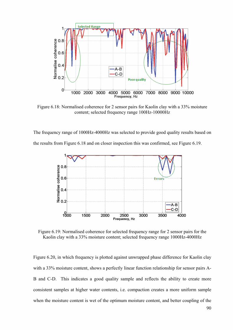
90
Figure 6.18: Normalised coherence for 2 sensor pairs for Kaolin clay with a 33% moisture content; selected frequency range 100Hz-10000Hz
The frequency range of 1000Hz-4000Hz was selected to provide good quality results based on
the results from Figure 6.18 and on closer inspection this was confirmed, see Figure 6.19.
Figure 6.19: Normalised coherence for selected frequency range for 2 sensor pairs for the Kaolin clay with a 33% moisture content; selected frequency range 1000Hz-4000Hz
Figure 6.20, in which frequency is plotted against unwrapped phase difference for Kaolin clay
with a 33% moisture content, shows a perfectly linear function relationship for sensor pairs A-
B and C-D. This indicates a good quality sample and reflects the ability to create more
consistent samples at higher water contents, i.e. compaction creates a more uniform sample
when the moisture content is wet of the optimum moisture content, and better coupling of the
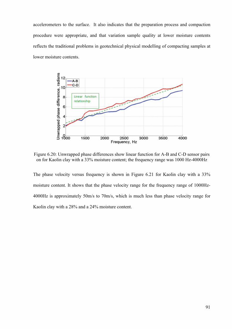
91
accelerometers to the surface. It also indicates that the preparation process and compaction
procedure were appropriate, and that variation sample quality at lower moisture contents
reflects the traditional problems in geotechnical physical modelling of compacting samples at
lower moisture contents.
Figure 6.20: Unwrapped phase differences show linear function for A-B and C-D sensor pairs on for Kaolin clay with a 33% moisture content; the frequency range was 1000 Hz-4000Hz
The phase velocity versus frequency is shown in Figure 6.21 for Kaolin clay with a 33%
moisture content. It shows that the phase velocity range for the frequency range of 1000Hz-
4000Hz is approximately 50m/s to 70m/s, which is much less than phase velocity range for
Kaolin clay with a 28% and a 24% moisture content.
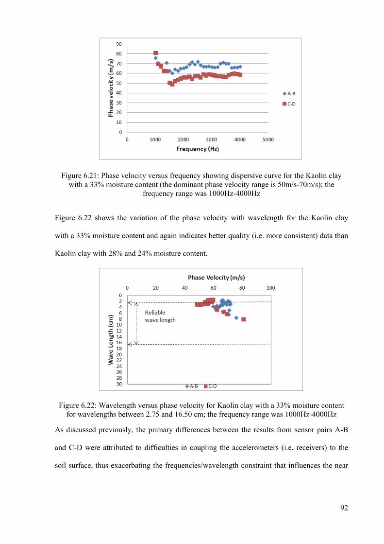
92
Figure 6.21: Phase velocity versus frequency showing dispersive curve for the Kaolin clay with a 33% moisture content (the dominant phase velocity range is 50m/s-70m/s); the
frequency range was 1000Hz-4000Hz
Figure 6.22 shows the variation of the phase velocity with wavelength for the Kaolin clay
with a 33% moisture content and again indicates better quality (i.e. more consistent) data than
Kaolin clay with 28% and 24% moisture content.
Figure 6.22: Wavelength versus phase velocity for Kaolin clay with a 33% moisture content for wavelengths between 2.75 and 16.50 cm; the frequency range was 1000Hz-4000Hz
As discussed previously, the primary differences between the results from sensor pairs A-B
and C-D were attributed to difficulties in coupling the accelerometers (i.e. receivers) to the
soil surface, thus exacerbating the frequencies/wavelength constraint that influences the near
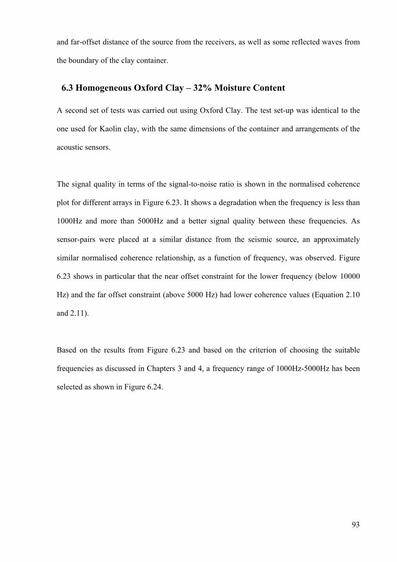
93
and far-offset distance of the source from the receivers, as well as some reflected waves from
the boundary of the clay container.
6.3 Homogeneous Oxford Clay – 32% Moisture Content
A second set of tests was carried out using Oxford Clay. The test set-up was identical to the
one used for Kaolin clay, with the same dimensions of the container and arrangements of the
acoustic sensors.
The signal quality in terms of the signal-to-noise ratio is shown in the normalised coherence
plot for different arrays in Figure 6.23. It shows a degradation when the frequency is less than
1000Hz and more than 5000Hz and a better signal quality between these frequencies. As
sensor-pairs were placed at a similar distance from the seismic source, an approximately
similar normalised coherence relationship, as a function of frequency, was observed. Figure
6.23 shows in particular that the near offset constraint for the lower frequency (below 10000
Hz) and the far offset constraint (above 5000 Hz) had lower coherence values (Equation 2.10
and 2.11).
Based on the results from Figure 6.23 and based on the criterion of choosing the suitable
frequencies as discussed in Chapters 3 and 4, a frequency range of 1000Hz-5000Hz has been
selected as shown in Figure 6.24.
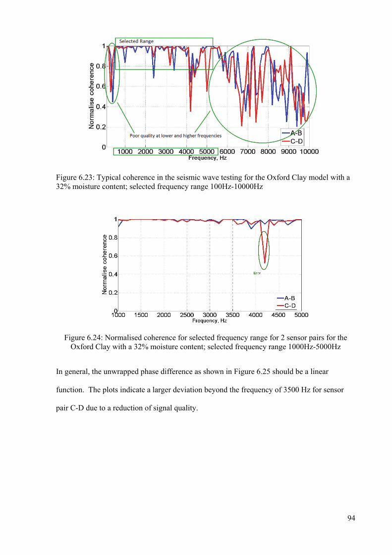
94
Figure 6.23: Typical coherence in the seismic wave testing for the Oxford Clay model with a 32% moisture content; selected frequency range 100Hz-10000Hz
Figure 6.24: Normalised coherence for selected frequency range for 2 sensor pairs for the Oxford Clay with a 32% moisture content; selected frequency range 1000Hz-5000Hz
In general, the unwrapped phase difference as shown in Figure 6.25 should be a linear
function. The plots indicate a larger deviation beyond the frequency of 3500 Hz for sensor
pair C-D due to a reduction of signal quality.

95
Figure 6.25: Unwrapped phase differences show and approximately linear function for A-B
and C-D sensor pairs for the Oxford Clay with a 32% moisture content for a frequency range of 1000Hz-5000Hz
Figure 6.26 shows a typical phase dispersion plot for one set of tests indicating that the phase
velocities are relatively consistent for frequencies between 1500Hz and 5000Hz. Uncommon
clay phase velocities were observed for frequencies below 1500Hz, which was likely caused
by the Rayleigh-waves being dominated by body waves and boundary reflections from a
longer wavelength. It indicates that the phase velocity range for the frequency range of
1500Hz-5000Hz is approximately 100m/s to 150m/s for Oxford Clay with a 32% moisture
content. Moreover based on these observations, phase velocities were reliable (i.e. close to
the mean value of phase velocity) when the data comply with the frequency or wavelength
requirement, even though the data have a low coherence threshold (0.9). It is worth to
underline that the measured values of phase wave velocities agree with typical values reported
in literature. MAdun et al., (2012), range phase wave velocity from 100 to 200 m/s.

96
Figure 6.26: Phase velocity versus frequency showing the dispersive curve for the Oxford Clay with a 32% moisture content; the frequency range was1000Hz-5000Hz
As mentioned earlier, there are two possible arrangements of seismic source and sensor-
receivers, namely seismic source at the one end of the array and seismic source at the middle
of the sensor-pairs. Based on the work of Madun (2011), in cases where the seismic source is
located at the middle of the array the source-receiver achieved higher signal-to-noise ratios
because both pairs of receivers are located closed to seismic source, there is a better
correlation of unwrapped phase difference between sensor-pairs and also observation of small
standard deviations demonstrates that this is an optimal arrangement for array deployment to
carry out the seismic surface wave test. This arrangement was therefore used in the test
programme.
In the case where the source was set in the middle of the array, the expected useful
frequencies for sensor pairs A-B and C-D were from 900Hz to 5400Hz based on calculations
using Equations 2.10 and 2.11. This is in agreement with the selected frequency range
obtained by trial and error in the first step of the test procedure.

97
Figure 6.27 is a plot of all data with no constraint on the coherence threshold. As was
mentioned before, this plot is important to evaluate the reliability of the phase velocity. To
avoid the far-offset constraint, the wavelengths should be larger than 2.75 cm (using Equation
2.11), and to avoid near-offset constraint the wavelengths should be below than 16.50 cm
(using Equation 2.10). Using these constraints the variation of average phase velocity versus
wavelength indicates a range of phase velocities between 100m/s and 150m/s.
Figure 6.27: Wavelength versus phase velocity for Oxford clay with a 32% moisture content for wavelengths of 2.75cm to 16.50 cm, corresponding to a frequency range of 1000 Hz-
5000Hz
This homogeneous soft clay is considered to have a constant phase velocity across its depth
due to its relatively uniform density profile both laterally and vertically (with depth) and the
phase velocities are therefore considered reliable. The phase velocities were converted into
shear wave velocities using Equation 3.9 (Vs(shear wave)=1.047.Vr(Rayleigh wave)) based
upon a Poisson’s ratio of 0.5 for the clay.
6.3.1 Repeatability of the tests - Oxford Clay
In order to test the repeatability of the experiments (i.e. to demonstrate that the measurement
system can give reliable results of phase velocities), a repeat test using Oxford Clay with a
moisture content of 32% was carried out using the same procedure as the first test for Oxford

98
Clay. As for the Kaolin clay repeat test, the plastic box was emptied and a new sample of clay
was mixed, and placed and compacted in the test bed. Figures 6.28 and 6.29 show the results
for Oxford Clay with a 32% moisture content as a repeated test. In the first test, the acceptable
frequency range was 1000Hz-5000Hz based on a coherence threshold of 0.9. Figure 6.28
indicates a slightly improved signal compared to the results in Figure 6.23.
Figure 6.28: Normalised coherence for 2 sensor pairs for the Oxford Clay with a 32%
moisture content (repeated test); selected frequency range 100Hz-10000Hz
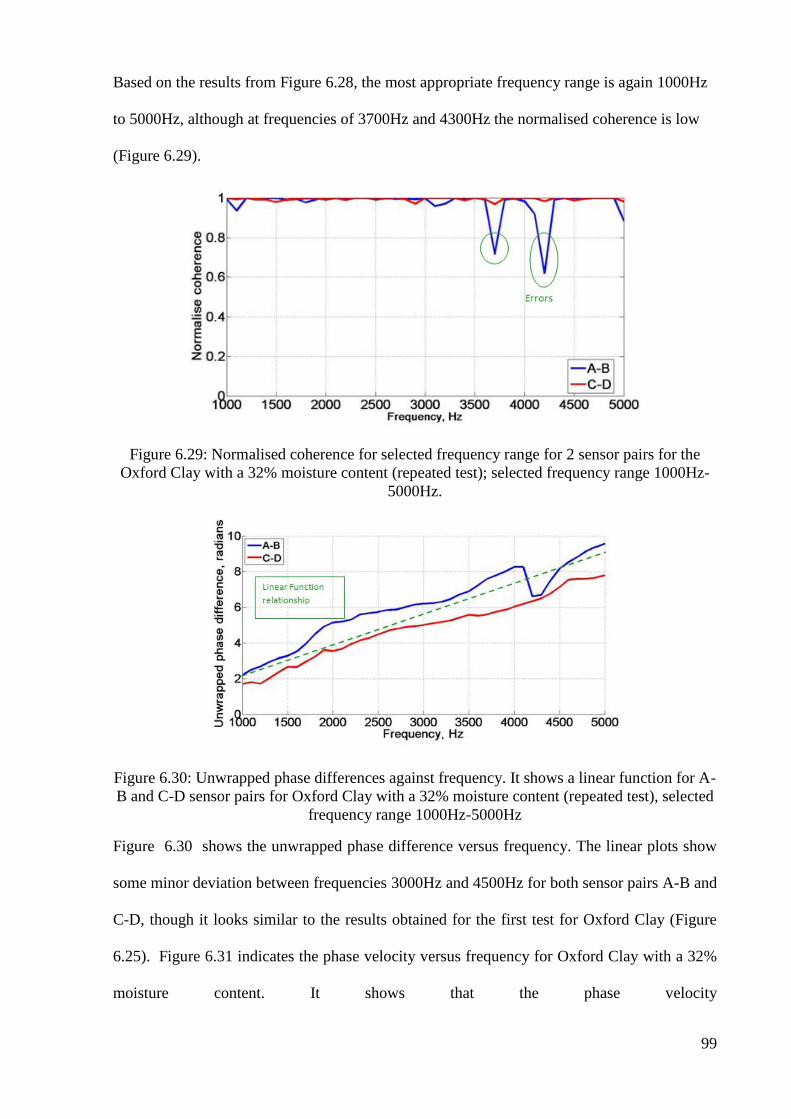
99
Based on the results from Figure 6.28, the most appropriate frequency range is again 1000Hz
to 5000Hz, although at frequencies of 3700Hz and 4300Hz the normalised coherence is low
(Figure 6.29).
Figure 6.29: Normalised coherence for selected frequency range for 2 sensor pairs for theOxford Clay with a 32% moisture content (repeated test); selected frequency range 1000Hz-
5000Hz.
Figure 6.30: Unwrapped phase differences against frequency. It shows a linear function for A-B and C-D sensor pairs for Oxford Clay with a 32% moisture content (repeated test), selected
frequency range 1000Hz-5000Hz
Figure 6.30 shows the unwrapped phase difference versus frequency. The linear plots show
some minor deviation between frequencies 3000Hz and 4500Hz for both sensor pairs A-B and
C-D, though it looks similar to the results obtained for the first test for Oxford Clay (Figure
6.25). Figure 6.31 indicates the phase velocity versus frequency for Oxford Clay with a 32%
moisture content. It shows that the phase velocity
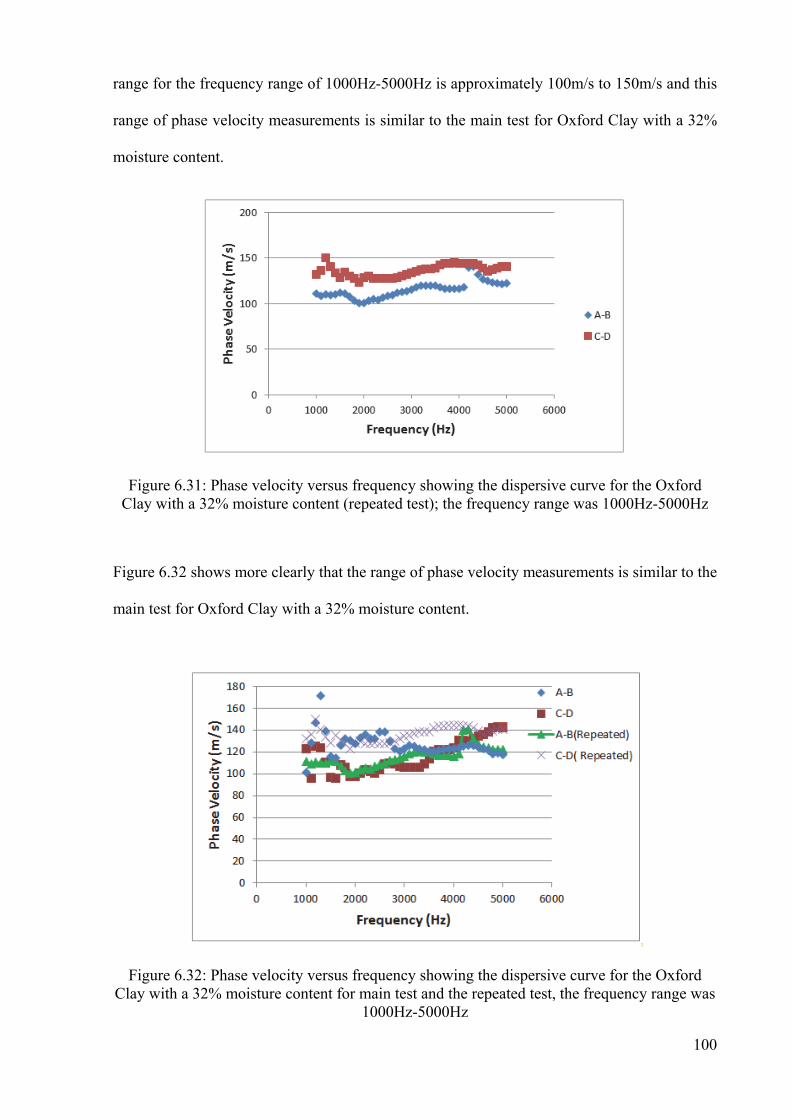
100
range for the frequency range of 1000Hz-5000Hz is approximately 100m/s to 150m/s and this
range of phase velocity measurements is similar to the main test for Oxford Clay with a 32%
moisture content.
Figure 6.31: Phase velocity versus frequency showing the dispersive curve for the Oxford Clay with a 32% moisture content (repeated test); the frequency range was 1000Hz-5000Hz
Figure 6.32 shows more clearly that the range of phase velocity measurements is similar to the
main test for Oxford Clay with a 32% moisture content.
Figure 6.32: Phase velocity versus frequency showing the dispersive curve for the Oxford Clay with a 32% moisture content for main test and the repeated test, the frequency range was
1000Hz-5000Hz
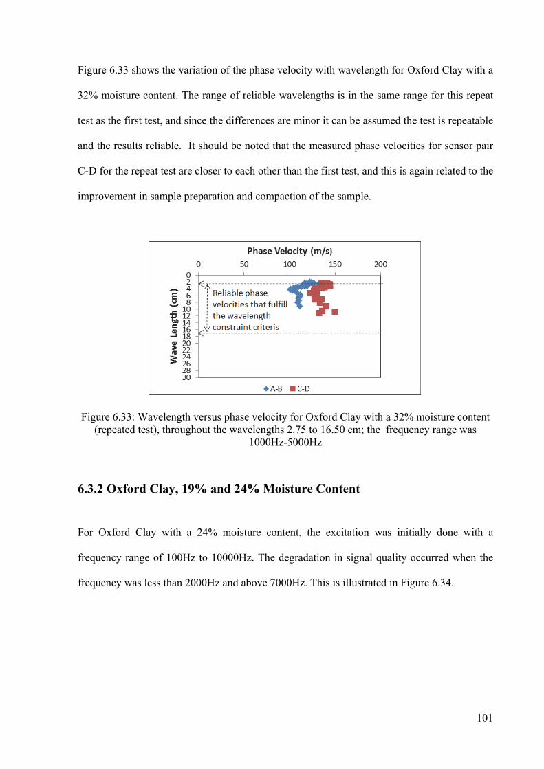
101
Figure 6.33 shows the variation of the phase velocity with wavelength for Oxford Clay with a
32% moisture content. The range of reliable wavelengths is in the same range for this repeat
test as the first test, and since the differences are minor it can be assumed the test is repeatable
and the results reliable. It should be noted that the measured phase velocities for sensor pair
C-D for the repeat test are closer to each other than the first test, and this is again related to the
improvement in sample preparation and compaction of the sample.
Figure 6.33: Wavelength versus phase velocity for Oxford Clay with a 32% moisture content (repeated test), throughout the wavelengths 2.75 to 16.50 cm; the frequency range was
1000Hz-5000Hz
6.3.2 Oxford Clay, 19% and 24% Moisture Content
For Oxford Clay with a 24% moisture content, the excitation was initially done with a
frequency range of 100Hz to 10000Hz. The degradation in signal quality occurred when the
frequency was less than 2000Hz and above 7000Hz. This is illustrated in Figure 6.34.
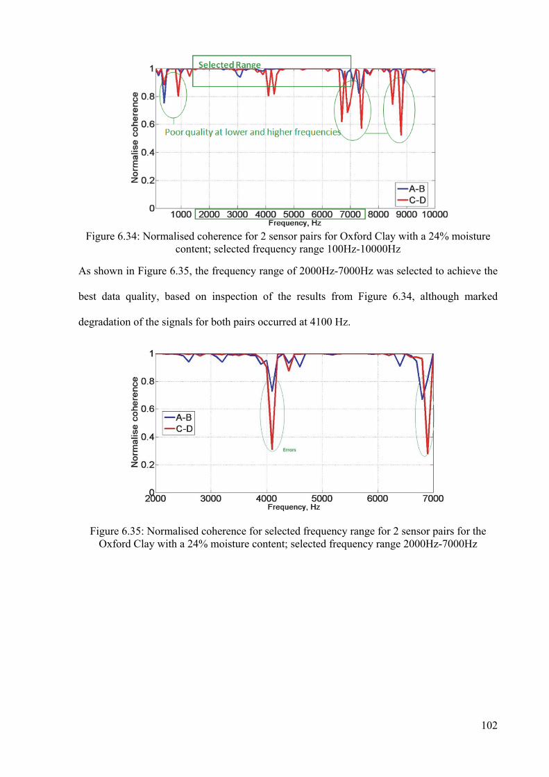
102
Figure 6.34: Normalised coherence for 2 sensor pairs for Oxford Clay with a 24% moisture
content; selected frequency range 100Hz-10000Hz
As shown in Figure 6.35, the frequency range of 2000Hz-7000Hz was selected to achieve the
best data quality, based on inspection of the results from Figure 6.34, although marked
degradation of the signals for both pairs occurred at 4100 Hz.
Figure 6.35: Normalised coherence for selected frequency range for 2 sensor pairs for the Oxford Clay with a 24% moisture content; selected frequency range 2000Hz-7000Hz
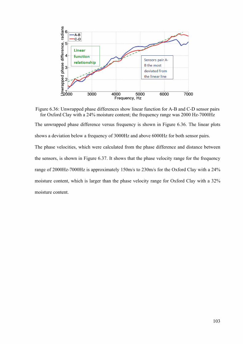
103
Figure 6.36: Unwrapped phase differences show linear function for A-B and C-D sensor pairs for Oxford Clay with a 24% moisture content; the frequency range was 2000 Hz-7000Hz
The unwrapped phase difference versus frequency is shown in Figure 6.36. The linear plots
shows a deviation below a frequency of 3000Hz and above 6000Hz for both sensor pairs.
The phase velocities, which were calculated from the phase difference and distance between
the sensors, is shown in Figure 6.37. It shows that the phase velocity range for the frequency
range of 2000Hz-7000Hz is approximately 150m/s to 230m/s for the Oxford Clay with a 24%
moisture content, which is larger than the phase velocity range for Oxford Clay with a 32%
moisture content.
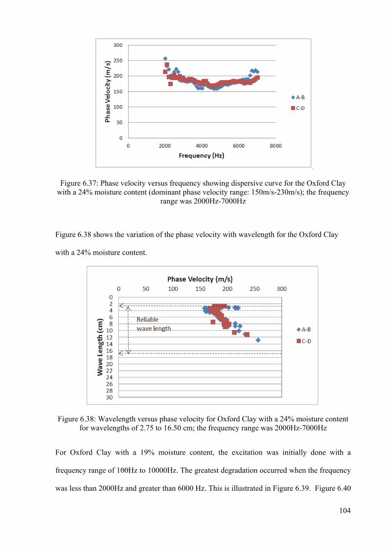
104
Figure 6.37: Phase velocity versus frequency showing dispersive curve for the Oxford Clay with a 24% moisture content (dominant phase velocity range: 150m/s-230m/s); the frequency
range was 2000Hz-7000Hz
Figure 6.38 shows the variation of the phase velocity with wavelength for the Oxford Clay
with a 24% moisture content.
Figure 6.38: Wavelength versus phase velocity for Oxford Clay with a 24% moisture content for wavelengths of 2.75 to 16.50 cm; the frequency range was 2000Hz-7000Hz
For Oxford Clay with a 19% moisture content, the excitation was initially done with a
frequency range of 100Hz to 10000Hz. The greatest degradation occurred when the frequency
was less than 2000Hz and greater than 6000 Hz. This is illustrated in Figure 6.39. Figure 6.40
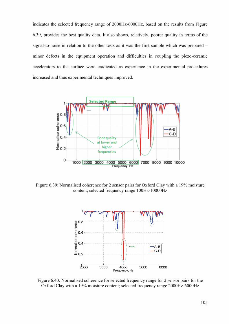
105
indicates the selected frequency range of 2000Hz-6000Hz, based on the results from Figure
6.39, provides the best quality data. It also shows, relatively, poorer quality in terms of the
signal-to-noise in relation to the other tests as it was the first sample which was prepared –
minor defects in the equipment operation and difficulties in coupling the piezo-ceramic
accelerators to the surface were eradicated as experience in the experimental procedures
increased and thus experimental techniques improved.
Figure 6.39: Normalised coherence for 2 sensor pairs for Oxford Clay with a 19% moisture
content; selected frequency range 100Hz-10000Hz
Figure 6.40: Normalised coherence for selected frequency range for 2 sensor pairs for the Oxford Clay with a 19% moisture content; selected frequency range 2000Hz-6000Hz

106
Figure 6.41 indicates frequency against unwrapped phase difference for Oxford Clay with a
19% moisture content. Although approximately linear, it shows a poorer quality relationship
for sensor pairs A-B and C-D than for wetter samples, which as mentioned relates to
difficulties in achieving uniformity in the preparation and compaction processes.
Figure 6.41: Unwrapped phase differences show linear function for A-B and C-D sensor pairs on for Oxford Clay with a 19% moisture content; the frequency range was 2000 Hz-6000Hz
The phase velocity versus frequency is shown in Figure 6.42 for Oxford Clay with a 19%
moisture content. It shows that the phase velocity range for the frequency range of 2000Hz-
6000Hz is approximately 250m/s to 320m/s, which as expected is more than the phase
velocity range for Oxford Clay with a 24% and a 32% moisture content. Figure 6.43 shows
the variation of the phase velocity with wavelength for the Oxford Clay with a 19% moisture
content. Interestingly these two figures show that the results even at this low water content
are more consistent than those for Kaolin clay at lower water contents.
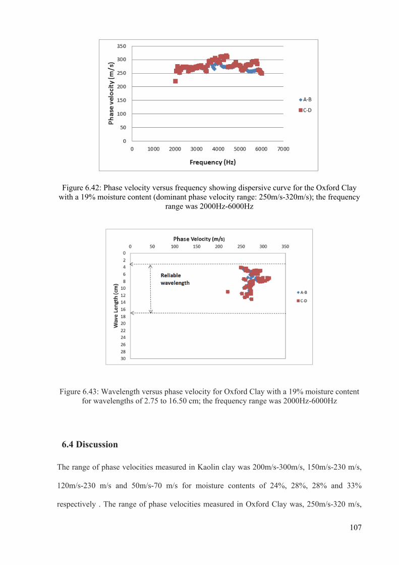
107
Figure 6.42: Phase velocity versus frequency showing dispersive curve for the Oxford Clay with a 19% moisture content (dominant phase velocity range: 250m/s-320m/s); the frequency
range was 2000Hz-6000Hz
Figure 6.43: Wavelength versus phase velocity for Oxford Clay with a 19% moisture content for wavelengths of 2.75 to 16.50 cm; the frequency range was 2000Hz-6000Hz
6.4 Discussion
The range of phase velocities measured in Kaolin clay was 200m/s-300m/s, 150m/s-230 m/s,
120m/s-230 m/s and 50m/s-70 m/s for moisture contents of 24%, 28%, 28% and 33%
respectively . The range of phase velocities measured in Oxford Clay was, 250m/s-320 m/s,
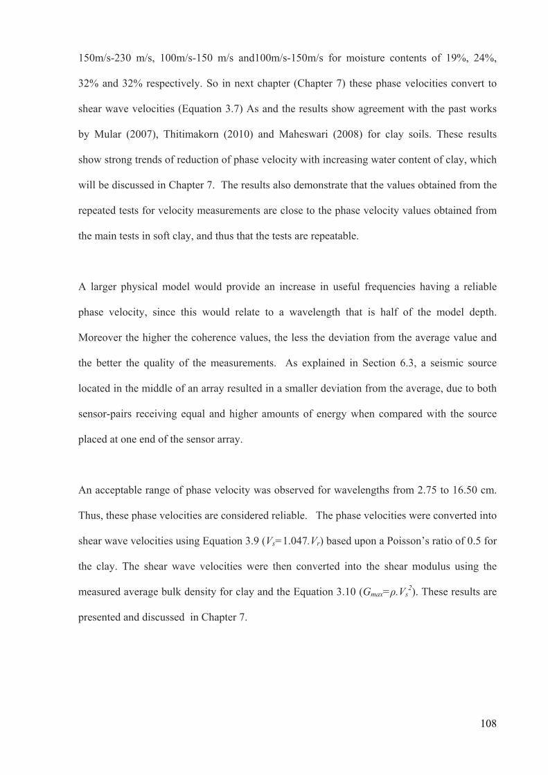
108
150m/s-230 m/s, 100m/s-150 m/s and100m/s-150m/s for moisture contents of 19%, 24%,
32% and 32% respectively. So in next chapter (Chapter 7) these phase velocities convert to
shear wave velocities (Equation 3.7) As and the results show agreement with the past works
by Mular (2007), Thitimakorn (2010) and Maheswari (2008) for clay soils. These results
show strong trends of reduction of phase velocity with increasing water content of clay, which
will be discussed in Chapter 7. The results also demonstrate that the values obtained from the
repeated tests for velocity measurements are close to the phase velocity values obtained from
the main tests in soft clay, and thus that the tests are repeatable.
A larger physical model would provide an increase in useful frequencies having a reliable
phase velocity, since this would relate to a wavelength that is half of the model depth.
Moreover the higher the coherence values, the less the deviation from the average value and
the better the quality of the measurements. As explained in Section 6.3, a seismic source
located in the middle of an array resulted in a smaller deviation from the average, due to both
sensor-pairs receiving equal and higher amounts of energy when compared with the source
placed at one end of the sensor array.
An acceptable range of phase velocity was observed for wavelengths from 2.75 to 16.50 cm.
Thus, these phase velocities are considered reliable. The phase velocities were converted into
shear wave velocities using Equation 3.9 (Vs=1.047.Vr) based upon a Poisson’s ratio of 0.5 for
the clay. The shear wave velocities were then converted into the shear modulus using the
measured average bulk density for clay and the Equation 3.10 (Gmax=ρ.Vs2). These results are
presented and discussed in Chapter 7.
109
Chapter 7
DISCUSSION
7.1 Introduction
This chapter discusses the results of the model testing for Kaolin Clay and Oxford Clay,
which aimed to develop the most appropriate seismic wave method to find the relationship
between geophysical and geotechnical properties of soil. Feasibility testing was conducted
(see Chapter 4) to establish the equipment and its system for surface wave testing at the
laboratory scale. Different materials were used in the main programme of testing in order to
achieve the aim of the study.
7.2 Equipment and System
The equipment used to create a steady state vibration source was a National Instruments (NI)
data acquisition system combined with an electromechanical vibrator and piezo-ceramic
transducer, used to produce the seismic wave energy to generate the transmission waveform,
which was amplified by the audio power amplifier. As reported in Chapter 3 the surface wave

110
was generated by a piezo-ceramic transducer with an electromechanical vibrator placed above
it, creating a point energy source (see Figure 3.3), and this was positioned in the centre of the
linear sequence of four receivers. On the output side four piezoelectric-accelerometers,
connected to a four channel signal conditioner, were used. The conversion of the seismic
wave energy to voltage was achieved using the NI analogue to digital converter module. This
equipment was connected to a personal computer and controlled from within the Matlab
environment. The outputs were stored for further processing.
The seismic surface wave system was designed to obtain a higher signal-to-noise ratio at a
selected frequency range, thus a stepped-frequency approach was preferred. Each frequency
step consisted of a few repetitive snapshots to improve the signal-to-noise ratio of the received
signal (Clayton, 2011).\The Matlab script developed for this project to run the system is
shown in Appendix B (1). Four sensors create two sensor-pairs, based on the symmetrical
arrangement of the seismic source and receivers. The stepped-frequencies data were processed
in Matlab environment as shown in Appendix B (2) and this was used to obtain phase
difference between sensor-pairs. To obtain the phase velocity for each sensor-pair and an
assessment of the quality of signal, which was represented by the coherence, further
processing of the received signal was needed as shown in Appendix B (3). A repeated test
was also introduced for improving the reliability of the calculated velocities.
7.3 Clay Model
7.3.1 Phase and Shear Wave Velocity Variations
7.3.1.1 Kaolin Clay
The initial water contents of Kaolin Clay were 24%, 28% and 33% and the associated range of
phase velocities measured was 200m/s-300m/s, 150m/s-230m/s and 50m/s-70m/s, as
discussed in Section 6.3. The experimental results of average phase velocity for Kaolin Clay
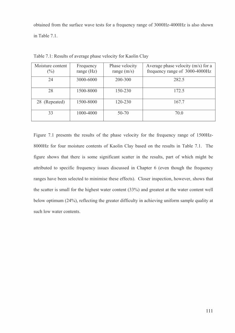
111
obtained from the surface wave tests for a frequency range of 3000Hz-4000Hz is also shown
in Table 7.1.
Table 7.1: Results of average phase velocity for Kaolin Clay
Moisture content (%)
Frequency range (Hz)
Phase velocity range (m/s)
Average phase velocity (m/s) for a frequency range of 3000-4000Hz
24 3000-6000 200-300 282.5
28 1500-8000 150-230 172.5
28 (Repeated) 1500-8000 120-230 167.7
33 1000-4000 50-70 70.0
Figure 7.1 presents the results of the phase velocity for the frequency range of 1500Hz-
8000Hz for four moisture contents of Kaolin Clay based on the results in Table 7.1. The
figure shows that there is some significant scatter in the results, part of which might be
attributed to specific frequency issues discussed in Chapter 6 (even though the frequency
ranges have been selected to minimise these effects). Closer inspection, however, shows that
the scatter is small for the highest water content (33%) and greatest at the water content well
below optimum (24%), reflecting the greater difficulty in achieving uniform sample quality at
such low water contents.

112
Figure 7.1: Results of the phase velocity versus frequency for the frequency range of 1500Hz-8000Hz for Kaolin Clay
Figure 7.2 shows the phase velocity variation for the frequency range of 3000Hz-4000Hz for
four moisture contents of Kaolin Clay based on the results from Table 7.1. The average phase
velocities are 282.5, 172.5 and 70.0m/s for moisture contents of 24%, 28% and 33%
respectively, which indicates that the phase velocity is decreasing while the moisture content
is increasing. The reason will be discussed later on this section.
Figure 7.2: Phase velocity variation for the frequency range of 3000Hz-4000Hz for Kaolin
Clay. As in mentioned before, the phase velocity can be converted to shear wave velocity
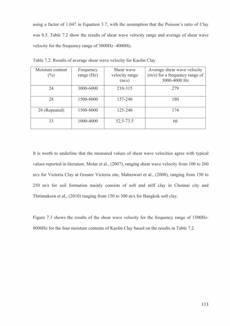
113
using a factor of 1.047 in Equation 3.7, with the assumption that the Poisson’s ratio of Clay
was 0.5. Table 7.2 show the results of shear wave velocity range and average of shear wave
velocity for the frequency range of 3000Hz -4000Hz.
Table 7.2: Results of average shear wave velocity for Kaolin Clay
Moisture content (%)
Frequency range (Hz)
Shear wave velocity range
(m/s)
Average shear wave velocity (m/s) for a frequency range of
3000-4000 Hz
24 3000-6000 210-315 279
28 1500-8000 157-240 180
28 (Repeated) 1500-8000 125-240 174
33 1000-4000 52.5-73.5 66
It is worth to underline that the measured values of shear wave velocities agree with typical
values reported in literature. Molar et al., (2007), ranging shear wave velocity from 100 to 260
m/s for Victoria Clay at Greater Victoria site, Maheswari et al., (2008), ranging from 150 to
250 m/s for soil formation mainly consists of soft and stiff clay in Chennai city and
Thitimakorn et al., (2010) ranging from 150 to 300 m/s for Bangkok soft clay.
Figure 7.3 shows the results of the shear wave velocity for the frequency range of 1500Hz-
8000Hz for the four moisture contents of Kaolin Clay based on the results in Table 7.2.
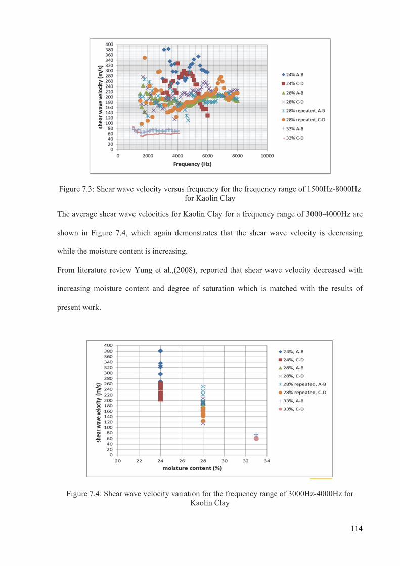
114
Figure 7.3: Shear wave velocity versus frequency for the frequency range of 1500Hz-8000Hz for Kaolin Clay
The average shear wave velocities for Kaolin Clay for a frequency range of 3000-4000Hz are
shown in Figure 7.4, which again demonstrates that the shear wave velocity is decreasing
while the moisture content is increasing.
From literature review Yung et al.,(2008), reported that shear wave velocity decreased with
increasing moisture content and degree of saturation which is matched with the results of
present work.
Figure 7.4: Shear wave velocity variation for the frequency range of 3000Hz-4000Hz for Kaolin Clay
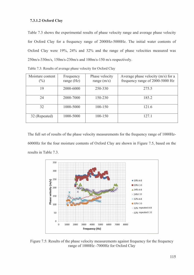
115
7.3.1.2 Oxford Clay
Table 7.3 shows the experimental results of phase velocity range and average phase velocity
for Oxford Clay for a frequency range of 2000Hz-5000Hz. The initial water contents of
Oxford Clay were 19%, 24% and 32% and the range of phase velocities measured was
250m/s-330m/s, 150m/s-230m/s and 100m/s-150 m/s respectively.
Table 7.3: Results of average phase velocity for Oxford Clay
Moisture content (%)
Frequency range (Hz)
Phase velocity range (m/s)
Average phase velocity (m/s) for a frequency range of 2000-5000 Hz
19 2000-6000 250-330 275.5
24 2000-7000 150-230 185.2
32 1000-5000 100-150 121.6
32 (Repeated) 1000-5000 100-150 127.1
The full set of results of the phase velocity measurements for the frequency range of 1000Hz-
6000Hz for the four moisture contents of Oxford Clay are shown in Figure 7.5, based on the
results in Table 7.3.
Figure 7.5: Results of the phase velocity measurements against frequency for the frequency range of 1000Hz -7000Hz for Oxford Clay
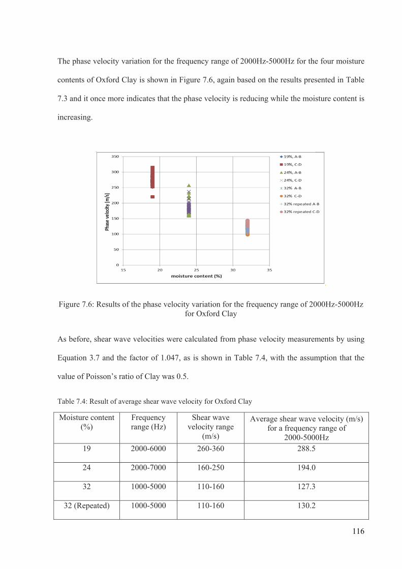
116
The phase velocity variation for the frequency range of 2000Hz-5000Hz for the four moisture
contents of Oxford Clay is shown in Figure 7.6, again based on the results presented in Table
7.3 and it once more indicates that the phase velocity is reducing while the moisture content is
increasing.
Figure 7.6: Results of the phase velocity variation for the frequency range of 2000Hz-5000Hz for Oxford Clay
As before, shear wave velocities were calculated from phase velocity measurements by using
Equation 3.7 and the factor of 1.047, as is shown in Table 7.4, with the assumption that the
value of Poisson’s ratio of Clay was 0.5.
Table 7.4: Result of average shear wave velocity for Oxford Clay
Moisture content (%)
Frequency range (Hz)
Shear wave velocity range
(m/s)
Average shear wave velocity (m/s) for a frequency range of
2000-5000Hz 19 2000-6000 260-360 288.5
24 2000-7000 160-250 194.0
32 1000-5000 110-160 127.3
32 (Repeated) 1000-5000 110-160 130.2

117
Same as Kaoli Clay table of results, the present table show a good match with the previous
works results in the literature, Mular (2007), Thitimakorn (2010) and Maheswari (2008),
which indicated range of 100 to 300 m/s for shear wave velocity for clay soils.
On the other hand Madun et al., (2012), measured shear wave velocity for Oxford clay with
32% moisture content at the same condition of sample preparation and testing method with
present work and show good agreement with measured shear velocity and shear modulus with
this work.
Figure 7.7 displays the results of the shear wave velocity for the frequency range of 1000Hz-
6000Hz for the four moisture contents of Oxford Clay based on the results in Table 7.4.
Figure 7.7: Results of shear wave velocity versus frequency for the frequency range of 1000Hz-7000Hz for Oxford Clay
The average shear wave velocities for Oxford Clay for the frequency range of 1000Hz-
6000Hz is shown in Figure 7.8, which again shows an obvious pattern of decreasing shear
wave velocity while the moisture content is increasing.

118
And same as before, from literature review Yung et al.,(2008), reported that shear wave
velocity decreased with increasing moisture content and degree of saturation which is
matched with the results of present work.
Figure 7.2 plots the relationship between phase velocity and moisture content, and Figure 7.4
the shear wave velocity versus moisture content, for a frequency range of 3000Hz-4000Hz for
Kaolin Clay. Figure 7.6 plots phase velocity against moisture content and Figure 7.8 shear
wave velocity against moisture content for the frequency range 2000Hz-5000Hz for Oxford
Clay. All these figures show phase velocity decreases with increasing moisture content of soil.
This behaviour can be attributed to influences of both the pore water in the soil and the soil
skeleton, i.e. wave propagation through saturated soils involves both the soil skeleton and
water in the void spaces. For S-wave propagation, the pore water has no resistance to shear
and thus the S-wave in soils is dependent only on the properties of the soil skeleton (Das,
1983), i.e. the ‘interconnectedness’ of the soil particles. Similar principles can be drawn from
the field of unsaturated soils, since the ability to resist shearing decrease when moisture
content in soils increases and because pore water has no capacity to resist shear then the effect
must be due to soil particle interconnectivity (the relevant phenomena being friction and
Figure 7.8: Results of the shear wave velocity for the frequency range of 2000Hz-5000Hz for Oxford Clay
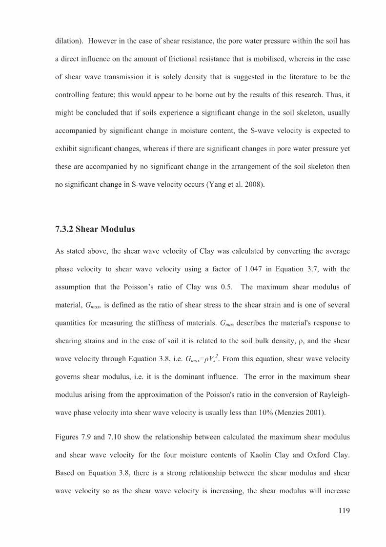
119
dilation). However in the case of shear resistance, the pore water pressure within the soil has
a direct influence on the amount of frictional resistance that is mobilised, whereas in the case
of shear wave transmission it is solely density that is suggested in the literature to be the
controlling feature; this would appear to be borne out by the results of this research. Thus, it
might be concluded that if soils experience a significant change in the soil skeleton, usually
accompanied by significant change in moisture content, the S-wave velocity is expected to
exhibit significant changes, whereas if there are significant changes in pore water pressure yet
these are accompanied by no significant change in the arrangement of the soil skeleton then
no significant change in S-wave velocity occurs (Yang et al. 2008).
7.3.2 Shear Modulus
As stated above, the shear wave velocity of Clay was calculated by converting the average
phase velocity to shear wave velocity using a factor of 1.047 in Equation 3.7, with the
assumption that the Poisson’s ratio of Clay was 0.5. The maximum shear modulus of
material, Gmax, is defined as the ratio of shear stress to the shear strain and is one of several
quantities for measuring the stiffness of materials. Gmax describes the material's response to
shearing strains and in the case of soil it is related to the soil bulk density, ρ, and the shear
wave velocity through Equation 3.8, i.e. Gmax=ρVs2. From this equation, shear wave velocity
governs shear modulus, i.e. it is the dominant influence. The error in the maximum shear
modulus arising from the approximation of the Poisson's ratio in the conversion of Rayleigh-
wave phase velocity into shear wave velocity is usually less than 10% (Menzies 2001).
Figures 7.9 and 7.10 show the relationship between calculated the maximum shear modulus
and shear wave velocity for the four moisture contents of Kaolin Clay and Oxford Clay.
Based on Equation 3.8, there is a strong relationship between the shear modulus and shear
wave velocity so as the shear wave velocity is increasing, the shear modulus will increase
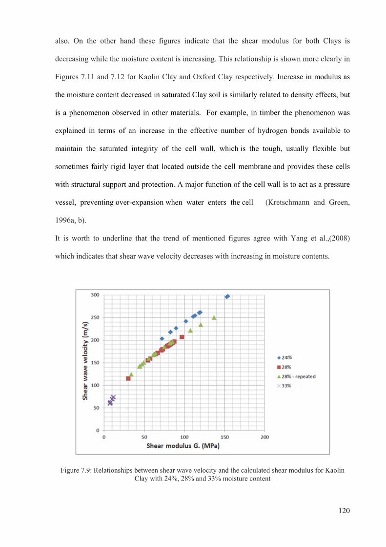
120
also. On the other hand these figures indicate that the shear modulus for both Clays is
decreasing while the moisture content is increasing. This relationship is shown more clearly in
Figures 7.11 and 7.12 for Kaolin Clay and Oxford Clay respectively. Increase in modulus as
the moisture content decreased in saturated Clay soil is similarly related to density effects, but
is a phenomenon observed in other materials. For example, in timber the phenomenon was
explained in terms of an increase in the effective number of hydrogen bonds available to
maintain the saturated integrity of the cell wall, which is the tough, usually flexible but
sometimes fairly rigid layer that located outside the cell membrane and provides these cells
with structural support and protection. A major function of the cell wall is to act as a pressure
vessel, preventing over-expansion when water enters the cell (Kretschmann and Green,
1996a, b).
It is worth to underline that the trend of mentioned figures agree with Yang et al.,(2008)
which indicates that shear wave velocity decreases with increasing in moisture contents.
Figure 7.9: Relationships between shear wave velocity and the calculated shear modulus for Kaolin Clay with 24%, 28% and 33% moisture content
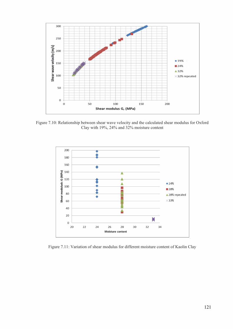
121
Figure 7.10: Relationship between shear wave velocity and the calculated shear modulus for Oxford Clay with 19%, 24% and 32% moisture content
Figure 7.11: Variation of shear modulus for different moisture content of Kaolin Clay
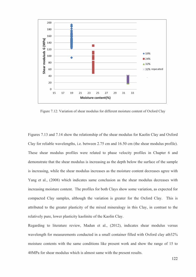
122
Figure 7.12: Variation of shear modulus for different moisture content of Oxford Clay
Figures 7.13 and 7.14 show the relationship of the shear modulus for Kaolin Clay and Oxford
Clay for reliable wavelengths, i.e. between 2.75 cm and 16.50 cm (the shear modulus profile).
These shear modulus profiles were related to phase velocity profiles in Chapter 6 and
demonstrate that the shear modulus is increasing as the depth below the surface of the sample
is increasing, while the shear modulus increases as the moisture content decreases agree with
Yang et al., (2008) which indicates same conclusion as the shear modulus decreases with
increasing moisture content. The profiles for both Clays show some variation, as expected for
compacted Clay samples, although the variation is greater for the Oxford Clay. This is
attributed to the greater plasticity of the mixed mineralogy in this Clay, in contrast to the
relatively pure, lower plasticity kaolinite of the Kaolin Clay.
Regarding to literature review, Madun et al., (2012), indicates shear modulus versus
wavelength for measurements conducted in a small container filled with Oxford clay atb32%
moisture contents with the same conditions like present work and show the range of 15 to
40MPa for shear modulus which is almost same with the present results.
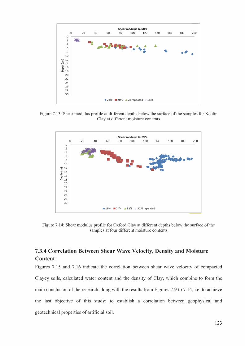
123
Figure 7.13: Shear modulus profile at different depths below the surface of the samples for Kaolin Clay at different moisture contents
Figure 7.14: Shear modulus profile for Oxford Clay at different depths below the surface of the samples at four different moisture contents
7.3.4 Correlation Between Shear Wave Velocity, Density and Moisture Content
Figures 7.15 and 7.16 indicate the correlation between shear wave velocity of compacted
Clayey soils, calculated water content and the density of Clay, which combine to form the
main conclusion of the research along with the results from Figures 7.9 to 7.14, i.e. to achieve
the last objective of this study: to establish a correlation between geophysical and
geotechnical properties of artificial soil.
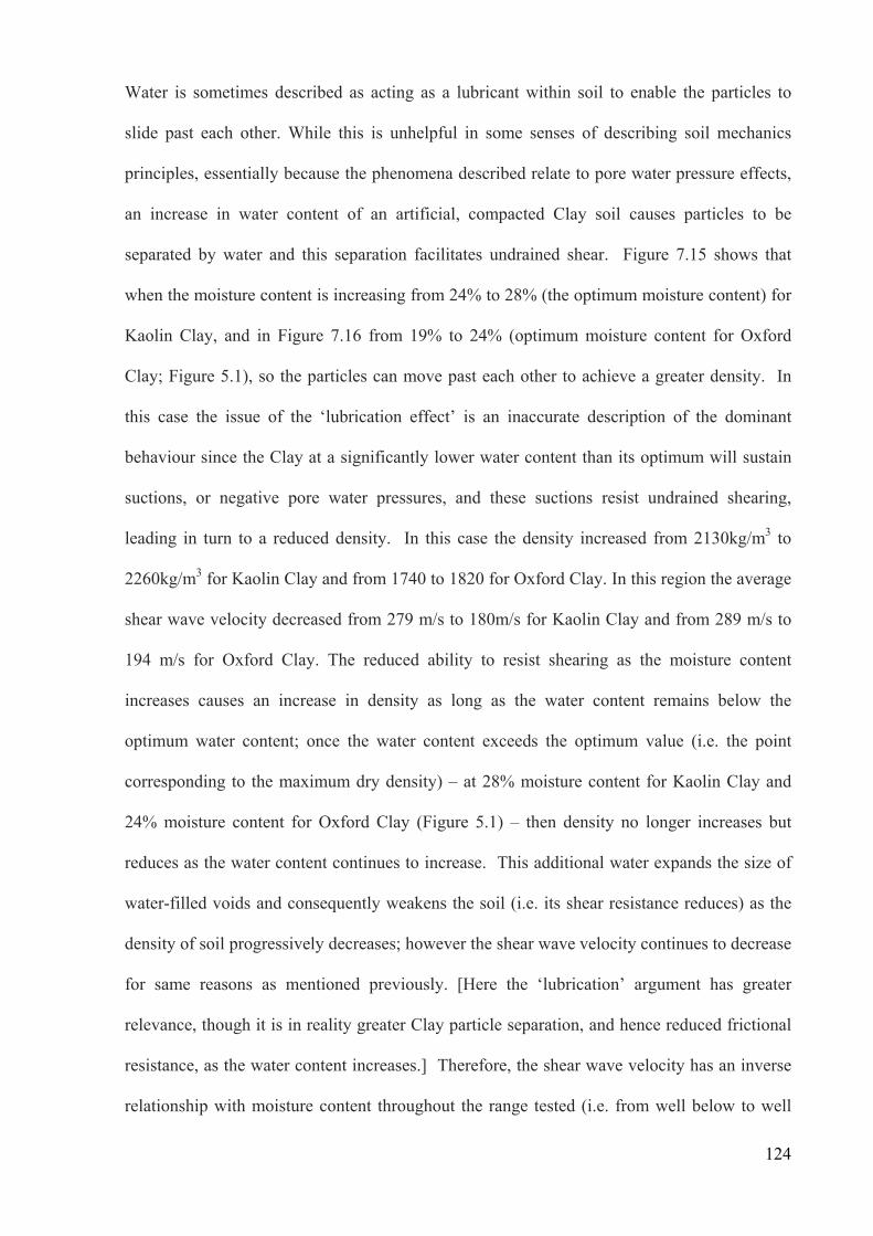
124
Water is sometimes described as acting as a lubricant within soil to enable the particles to
slide past each other. While this is unhelpful in some senses of describing soil mechanics
principles, essentially because the phenomena described relate to pore water pressure effects,
an increase in water content of an artificial, compacted Clay soil causes particles to be
separated by water and this separation facilitates undrained shear. Figure 7.15 shows that
when the moisture content is increasing from 24% to 28% (the optimum moisture content) for
Kaolin Clay, and in Figure 7.16 from 19% to 24% (optimum moisture content for Oxford
Clay; Figure 5.1), so the particles can move past each other to achieve a greater density. In
this case the issue of the ‘lubrication effect’ is an inaccurate description of the dominant
behaviour since the Clay at a significantly lower water content than its optimum will sustain
suctions, or negative pore water pressures, and these suctions resist undrained shearing,
leading in turn to a reduced density. In this case the density increased from 2130kg/m3 to
2260kg/m3 for Kaolin Clay and from 1740 to 1820 for Oxford Clay. In this region the average
shear wave velocity decreased from 279 m/s to 180m/s for Kaolin Clay and from 289 m/s to
194 m/s for Oxford Clay. The reduced ability to resist shearing as the moisture content
increases causes an increase in density as long as the water content remains below the
optimum water content; once the water content exceeds the optimum value (i.e. the point
corresponding to the maximum dry density) – at 28% moisture content for Kaolin Clay and
24% moisture content for Oxford Clay (Figure 5.1) – then density no longer increases but
reduces as the water content continues to increase. This additional water expands the size of
water-filled voids and consequently weakens the soil (i.e. its shear resistance reduces) as the
density of soil progressively decreases; however the shear wave velocity continues to decrease
for same reasons as mentioned previously. [Here the ‘lubrication’ argument has greater
relevance, though it is in reality greater Clay particle separation, and hence reduced frictional
resistance, as the water content increases.] Therefore, the shear wave velocity has an inverse
relationship with moisture content throughout the range tested (i.e. from well below to well

125
above the optimum water content), while it has an inverse relation with density before it
reaches the optimum water content (or maximum dry density) after which they exhibit a direct
relationship – which means that the shear wave velocity decreases while the density
decreases.
Figure 7.15: Variation of shear wave velocity related to moisture content and density of Kaolin Clay
In the literature it is suggested that a strong direct relationship exists between shear wave
velocity and density; (Clayton et al., 1995; Menzies and Matthews, 1996;
Massarsch, 2005), but it is contended that this is because of the limited range of water
contents over which this is observed and in natural soils at water contents below the optimum
Figure 7.16: Variation of shear wave velocity related to moisture content and density of Oxford Clay

126
water content, yet for compacted soils at water contents well above optimum the relationship
does not hold. In this research it is demonstrated that the strong relationship is in fact an
inverse relationship with water content. It is for this reason that the shape of the relationship
in Figures 7.15 and 7.16 resemble the typical shape of the standard compaction curves for
Clay soil (Figure 5.1).
127
Chapter 8
CONCLUSIONS AND RECOMMENDATIONS FOR
FURTHER RESEARCH
8.1 Introduction
In this thesis, the seismic surface wave technique has been described and relevant literature
reviewed. By way of laboratory testing, alternative test arrangements were examined and a
suitable testing programme was developed to meet the aim of developing an appropriate
seismic surface wave experimental methodology to assess how soil properties influence
seismic waves transmission and how they can be used to develop correlations between
acoustic and geotechnical properties. A test bed was established using two different types of
clay, Kaolin clay and Oxford Clay, with moisture contents varying from well above to well
below the optimum moisture contents.
It was clear from the literature review that a detailed programme of work was needed, based
in the laboratory, to assess the properties of soil in relation to surface shear wave
characteristics over this range of moisture contents. The equipment and system reliability

128
performance were established and checked, prior to the models of Kaolin clay and Oxford
Clay being tested.
Based on the results and experience gathered from the laboratory work, this chapter
summarizes the main findings and gives recommendations for future research. This work
focused on laboratory scale models, so providing essential parameter and boundary control.
From this work ways to adapt approaches for full-scale field testing, and ultimately quality
assurance testing, can be developed.
8.2 Main Outcomes
• From a laboratory point of view the selected size of the container/box was sufficiently
large to enable clay samples of a suitable quality to be made, i.e. placed and compacted well
and uniformly. Also it was acceptable from practical viewpoint, in terms of mixing and
handling the clay, but there were limitations from the acoustic experimentation point of view
so a specific frequency range for each clay type and water content had to be established to
ensure reliable results as follows. Despite careful prior consideration with regard to the size of
the container, some interference of the surface waves (these were the ones of interest in the
experiments) with body waves (near offset constraint effect) occurred. In addition,
attenuation of the surface waves (far offset constraint effect) was visible. These were
identified via the anomalies in the phase-response of the coherence plot and unwrapped phase
difference. A weaker signal quality at higher frequencies was due to a more rapid attenuation
of the shorter wavelengths as well as the presence of relatively strong boundary reflections,
thus reducing the signal quality at higher frequencies and deviation of associated phase
velocities. The sensors which were located further from the source received less energy,
which compromised signal quality under certain circumstances, and this problem was
exacerbated by the interfering reflected wave from the boundary of the container. For this
reason only reliable wavelengths, established via detailed initial analysis of the test data, were

129
considered when analyzing the results for this test model. A common problem with
geotechnical model testing, this research showed that by minimizing the size of sample some
parameters become more accurate, such as those associated with uniform compaction of the
sample, while on the other hand there will be some limitation on the range of reliable
wavelengths that can be used, e.g. because of the boundary reflections.
• The optimal arrangement of the sensor array on the test model was when the seismic
source was located at the centre of the array with the receiver pairs at either side. This
arrangement was based on the literature and previous work by Madun (2011). This
arrangement ensures that both sensor-pairs receive an equal and relatively high amount of
energy so that there is a relatively small deviation in the phase velocities. For the laboratory
seismic surface wave array set-up, the optimal distances between the source and the first
sensor (d) and sensors spacing (Δx) were 5.5cm and 2.5cm respectively. This array gave
reliable wavelengths between 2.75cm and 16.50cm, which were derived from half d and three
times d, respectively.
• During the tests it became apparent that a careful identification and selection of
suitable frequencies for each test was essential. The coherence plots gave an initial indication
of suitable frequencies, but closer inspection was required by looking at smaller frequency
bands as well as the graph of frequency against unwrapped phase difference. This indicated
frequency ranges where the confidence in the corresponding phase and ultimately shear wave
velocities is reduced.
• The data were recorded by two receiver pairs A-B and C-D. As the receiver pairs
were exactly the same distance from the seismic wave source, the signals should be identical
assuming the clay was homogenous and all other boundary conditions were identical.
However, looking at the data, and assuming that any differences were not due to experimental
130
influences such as sensor-clay coupling effects, it became apparent that there was some
variation between the two signals received indicating that, despite every effort, the clay was
not exactly homogenous with some variation throughout the container. The results were,
however, sufficiently similar to give confidence in the accuracy of the outcomes.
• The measurements of shear wave velocity and moisture content of clay soil show a
clear trend of reduction of shear wave velocity, and hence shear modulus, while the moisture
content is increasing for both clay test models over the full range of water contents tested, i.e.
from significantly wet through to significantly dry of the optimum water content.
• The measurements of shear wave velocity, moisture content and density of the clay
soils tested show that the shear wave velocity, and hence shear modulus, has an inverse
relationship with density before it reaches the optimum water content (or maximum dry
density) after which it exhibits a direct relationship, i.e. the shear wave velocity decreases
while the density decreases.
8.3 Recommendations for Future Research
• If the soil water contents and densities change with depth in a soil, as might occur with
traditionally compacted clay soils, the wavelength might not be equal to the depth. Therefore,
the relationship between the wavelength and the depth might be explored in a larger test
programme in which larger soil samples are included. However the maximum information on
the soil properties is limited to half of the model depth while the limitation arising from the
arrangement of the equipment (the distance of seismic source to the first receiver, d, and the
spacing between receivers, Δx) also needs consideration. The benefit from a larger d is the
acquisition of information from a deeper layer, yet a larger d causes a lower signal-to-noise
ratio and less information for the shallow layer.

131
• It would be beneficial to conduct seismic tests using bender elements to validate the seismic
surface wave results. [This was an original intention of this research, but repeated equipment
malfunctions precluded its use and the test programme presented herein was devised to
achieve the project’s objectives without bender elements.]
• Field measurements are ultimately required to validate the measurement technique established
in the laboratory. These might be carried out under a programme of research such as Mapping
the Underworld.
• The shear modulus profile established from the seismic test could be validated via computer
modelling.

132
REFERENCES
Abu-Hassanein, Z.S., Benson, C.H. and Blotz, L.R. (1996) Electrical resistivity of compacted clay. Journal of Geotechnical Engineering, ASCE, 122(5):397-406.
Adamo, F., Andria, G., Attivissimo, F., Giaquinto, N. (2004) An acoustic method for soil moisture measurement, IEEE Trans. Instrum. Meas. 891-898.
Adamo, F., Attivissimo, F., Fabbiano, L., Giaquinto, N. (2009) Velocity moisture relationship for sandy soil: Experimental results and data analysis 58 (2), 311-317.
Addo, K.O. and Robertson, P.K. (1992) Shear-wave velocity measurement of soils using Rayleigh waves. Canadian Geotechnical Journal, 29(4): 558-568.
Andrus, RD, Stokoe, KH. (2000). Liquefaction resistance of soils from shearwave velocity. Geotech Geoenviron Eng 2000;126(11):1015–25.
Al-Hunaidi M.O. (1993) Insight on the SASW non-destructive testing method. Canadian Geotechnical Journal, 20: 940–950.
Arulanandan, K and Muraleetharan, K (1988) Level ground soil-liquefaction analysis using in-situ properties. Journal Geotechnical Engineering ASCE, 114(7): 753-770
Asaka, Y and Abe, T. (2011) Non-destructive technique for assessing cement-treated ground. Ground Improvement, 164 (G13): 179–187.
Ashford, S.A., W. Jakrapiyanun and P. Lukkunaprasit, (1997). Amplification of earthquake ground
motions in Bangkok, Bangkok, Chulalonglongkorn University.
Atkinson, J. (2007) The mechanics of soils and foundations. 2nd edition. Oxon: Taylor and Francis.
BSI (1990) Methods of Test for Soils for Civil Engineering Purposes BS1377. London: British Standards Institution.
Cassidy, N.J. (2007) Frequency-dependent attenuation and velocity characteristics of magnetically lossy materials.In IEEE Proceedings of the 4th International Workshop on Advanced Ground Penetrating Radar, Naples, pp. 142–146.
Chan C.M. (2006) A laboratory investigation of shear wave velocity in stabilized soft soils. PhD thesis, University of Sheffield.
Christopher D.P. Baxter, P.E., M.ASCE; M.S. Ravi Sharma , Shear wave velocity of weakly cemented sand during drained and undrained triaxial compression . Civil and Environmental Engineering, The University of Rhode Island, Narraganset
Chen Yunmin C., , Han k., Ren-peng c., (2005). Correlation of shear wave velocity with liquefaction resistance based on laboratory tests. Civil Engineering Department, Institute of Geotechnical Engineering, Zhejiang University, Hangzhou Charles, J.A. and Watts, K.S. (2002) Treated ground engineering properties London: Construction Industry Research and Information Association, ClRlA C572.
133
Clayton, C.R.I. (2011) Stiffness at small strain: research and practice. Géotechnique, 61 (1): 5-37.
Clayton, C.R.I., Matthews, M.C. and Simons, N.E. (1995) Site Investigation. 2nd edition. London: Blackwell Science Ltd.
Cosenza, P., Marmet, E., Rejiba F., Cui, Y.J., Tabbagh, A. and Charlery, Y. (2006) Correlations between geotechnical and electrical data: A case study at Garchy in France. Journal of Applied Geophysics, 60 (2006): 165–178.
Crice, D. (2005) MASW: the wave of the future. Journal of Environmental and Engineering Geophysics, 10(2): 77–79.
Das, B .M. (1983) Fundamental of Soil Dynamics: Elsevier, New York.
Davich, P., Labuz, F.L., Guzina, L. And Drescher (2004)A small strain and resilient modulus testing of granular soils. Department of Transportation, University of Minnesota, August 2004.
Finck, F. (2003) Introduction of a ground penetrating radar system for investigations on concrete structures. 35 Otto-Graf-Journal Vol. 14, 2003.
Garcia-Bengochea, I., Lovell, C. and Altschaeffl (1979) Pore Distribution and permeability of silty clay. Journal of Geotechnical Engineering, ASCE, 105 (7): 839-856.
Giao P.H., Chung S.G., Kim D.Y., and Tanaka, H. (2003) Electric imaging and laboratory testing for geotechnical investigation of Pusan clay deposits. Journal of Applied Geophysics, 52 (2003): 157-175.
Gordon, M.A., Clayton, C.R.I., Thomas, T.C. and Matthews, M.C. (1996) The selection in interpretation of seismic geophysical methods for site investigation.In: Craig, C. (ed) Advances in site investigation practice. London: Thomas Telford. pp. 727-738.
Griffiths, D.H. and King, R.F. (1965) Applied geophysics for geologist and engineers. 2nd edition. Pergamon press,Oxford, UK.
Hardin, B.O., Black, W.L., (1968). Vibration modulus of normally consolidated clay. Journals of Soil Mechanics and Foundations Division ASCE 94 (SM2), 353–369. Hardin, B.O., Drnevich, V.P., (1972). Shear modulus and damping in soils. Journal of the Soil Mechanics and Foundations Division ASCE 98 (SM7), 667–692. Head, K.H. (1986) Manual of soil laboratory testing. Volume 3.. London: Pentech Press.
Heisey, J.S., Stokoe, K.H., and Meyer, A.H. (1982) Moduli of pavement systems from spectral analysis of surface waves. In Strength and deformation characteristics of pavements. Transportation Research Record 852, Washington, D.C., pp. 22–31.
shear-wave velocity structure beneath the Fraser River delta sediments – Preliminary results, Proceedings 8 th Canadian Conference on Earthquake Engineering, 101-106.
Hunter, J. A., H. A. Christian, J. B. Harris, J. R. Britton, and J. L. Luternauer, (1999). Mapping
134
Ifeachor E.C. and Jervis B.W. (1993) Digital signal processing: a practical approach. Addison: Wesley Publishing, 184-191.
University of Birmingham
Kramer, S.L. (1996)Geotechnical Earthquake Engineering. New JERSEY: Prentice-Hall International Series.
Keller, G. and Frischknecht, F. (1966) Electrical methods in geophysical prospecting. New York: Pergamon Press.
Kretschmann, D.E. and Green, D.W. (1996a)Moisture Content-Specific Gravity Relationship for Clear Southern Pine, In: Gopu, K.A. Vijaya, ed. Proceedings of the international wood engineering conference; 1996 October 28-31; New Orleans, LA. Baton Rouge, LA: Louisiana State University: Vol. 2: 536-542.
Kretschmann, D.E. and Green, D.W. (1996b). Modelling Moisture Content-Mechanical Property Relationships for Clear Southern Pine, Wood and Fiber Science, 28(3) : 320-337
Lankston, R.W. (1990) High-resolution refraction seismic data acquisition and interpretation. In Ward, S.H. (ed) Investigations in Geophysics no. 5, Volume 1: Review and Tutorial. Oklahoma: Society of Exploration Geophysicists. pp. 1-30.
Lee, L. (2001) Soil-pile interaction of bored and case in-situ piles. PhD Thesis, University of Birmingham.
Luke, B. (1999) Site investigations function better with seismic waves. IEEE Potentials, 18(1), Feb.-March 1999: 33-35.
Luna, R. and Jadi, H. (2000) Determination of dynamic soil properties using geophysical methods. In Proceedings of the First International Conference on the Application of Geophysical and NDT Methodologies to Transportation Facilities and Infrastructure, St. Louis, December 2000, pp. 1-15.
Madun, A. (2011)Seismic evaluation of vibro-stone column. PhD thesis, University of Birmingham.
Madun, A., Jefferson, I., Chapman, D.N., Culshaw, M.G., Foo K.Y. and Atkins, P.R. (2010a) Evaluation of the multi-channel surface wave analysis approach for the monitoring of multiple soil-stiffening columns. Near Surface Geophysics, 8(6): 611-621.
Madun, A., Jefferson, I., Foo, K.Y.,Chapman, D.N., Culshaw, M.G., Atikins, P.R. (2012) Laboratory scale seismic surface wave testing for the determination of soil elastic profiles, International Journal of Integrated Engeenireng, Vol. 4 No. 2 P 9-24
Massarsch K.R. (2005) Deformation properties of stabilized soil columns. In Proceedings International Conference on Deep Mixing, Stockhom, 23 - 25 May 2005.
Matthews M.C., Hope V.S. and Clayton C.R.I. (1995) The geotechnical value of ground stiffness determined using seismic methods. Geological Society, London, Engineering Geology Special
Inazaki ,T. (2006) , Relationship between S-Wave Velocities and Geotechnical Properties Of Alluvial Sediments. Public Works Research Institute, Tsukuba, JAPAN John, U.E. (2011) Chemical performance of cement stabilised contaminated clay. PhD thesis,

135
Publications, 12: 113-123.
Matthews, M.C. Hope, Y.S. and Clayton, C.R.I. (1996) The use of surface waves in the determination of ground stiffness profiles. Proceedings of the Institution of Civil Engineers Geotechnical Engineering, 119: 84-95.
Matthews, M.C., Clayton, C.R.I. and Own, Y. (2000) The use of field geophysical techniques to determine geotechnical stiffness parameters. Proceedings of the Institution of Civil Engineers Geotechnical Engineering, 143: 31-42.
Mattsson, H., Larsson, R., Holm, G., Dannewitz, N. and Eriksson, H. (2005) Down-hole technique improves quality control on dry mix columns. In Proceedings of the International Conference on Deep Mixing Best Practice and Recent Advances, Stockholm, Sweden, Vol. 1, pp. 581-592.
McDowell, P.W., Barker, R.D. and Butcher, A.P., et al. (2002) Geophysics in engineering investigations. London: Construction Industry Research and Information Association, ClRlA C562.
Menzies B.K. (2001) Near-surface site characterisation by ground stiffness profiling using surface wave geophysics. In Instrumentation in Geotechnical Engineering (eds K.R. Saxena and V.M. Sharma), H.C.Verma Commemorative Volume, 43-71. Oxford& IBH Publishing Co. Pvt. Ltd., New Delhi, Calcultta.
Menzies, B. and Matthews, M. (1996) The continuous surface-wave system: A modern technique for site investigation.In Special lecture: Indian Geotechnical Conference Madras, December 11-14th 1996.
Milsom, J. (1939) Field geophysics, The geological field guide series. 3rd edition. London,UK: John Wiley & sons Ltd. 12-13.
Moxhay, A.L., Tinsley, R.D. and Sutton J.A. (2001) Monitoring of soil stiffness during ground improvement using seismic surface waves. Ground Engineering Magazine, January: 34-37.
Moxhay, A.L., Tinsley, R.D., Redgers, J.D. and Gravell, D.C. (2008) The prediction of ground settlement from continuous surface wave data. Ground Engineering Magazine, July: 34-38.
Ohkubo, T., Terasaki, A., (1976). Physical Property and Seismic Wave Velocity of Rock. Oyo Corp. Park, C.B., Miller, R.D. and Xia, J. (2007) Multichannel Analysis Of Surface Waves (MASW)-Active And Passive Methods. The Leading Edge, January 2007, 60-64.
Park, C.B., Miller, R.D., and Xia, J. (1999) Multichannel analysis of surface waves. Geophysics,
Molnar S., Cassidy J.F.,. Monahan P.A., and Dosso S.E. (2007). Comparison Of Geophysical Shear-Wave Velocity Methods, Ninth Canadian Conference on Earthquake Engineering Ottawa, Ontario, Canada 26-29 Monahan, P. A., and V. M. Levson, (2001). Development of a shear-wave velocity model of the near surface deposits of southwestern British Columbia, Canada, 4th International Conference in Earthquake Engineering and Soil Dynamics, San Diego, California, 26-31 Monahan, P. A., and V. M. Levson,( 2000). Quaternary Geological Map of Greater Victoria. British Columbia Geological Survey, Ministry of Energy and Mines, Victoria, B.C.

136
64(3): 800-808.
Park, C.B., Miller, R.D., Ryden, N., Xia, J., and Ivanov, J., (2005) Combined use of active and passive surface waves. Journal of Engineering and Environmental Geophysics, 10 (3): 323-334.
Parasnis, D.S. (1962) Principles of applied geophysics. 5th edition. Thomas Press, New Dehli.
Pickett, G.R., (1963). Acoustic character logs and their applications in formation evaluation. Journal of Petroleum Technology 15, 650–667. Rampello. S., Viggiani, G. M. B. & Amorosi, A. (1997). Small-strain stiffness of reconstituted clay compressed along constant triaxial effective stress ratio paths. Geotechnique 47, No. 3, 475– 489. Redges, J.D., Moxhay, A.L., Ghataora, G.S. and Jefferson, I. (2008) Case histories of settlement performance comparisons on ground improvements using stiffness, seismic waves and traditional methods. In Proc. 6th International Conference on Case Histories in Geotechnical Engineering, Arlington, VA, 11-16 August 2008, Expanded Abstracts.
Reynolds, J.M. (1997) An introduction to applied and environmental geophysics. John Wiley & Sons.
Rhazi, J., Hassaim, M., Ballivy, G. and Hunaidi, O. (2002) Effects of concrete non-homogeneity on Rayleigh waves dispersion. Magazine of Concrete Research, 2002, 54, No. 3, June, 193–201.
Richart, F.E., Wood, R.D., Hall, J.R. (1970) Vibration of soils and foundations. New Jersey: Prentice-Hall.
Roy, D.R.N. (2010) Continuous surface wave testing of vibro-stonecolumn ground improvement. MSc thesis, University of Birmingham.
Sheriff, R.E. and Geldart, L.P. (1982) Exploration seismology, volume 1. Cambridge University Press.
Shibuya, S. and Tanaka, H. (1996) Estimate of elastic shear modulus in Holocene soil deposits. Soil Fdns, 36(4): 45-55.
Socco, L.V. and Strobbia, C. (2004) Surface wave method for near-surface characterization: a tutorial. Near Surface Geophysics, 2004, 165-185.
Staab, D.A., Edil, T.B. and Alumbaugh, D.L. (2004) Non-Destructive Evaluation of Cement-Mixed Soils. In Drilled Shafts, Micropiling, Deep Mixing, Remedial and Specialty Foundation Systems, Geotechnical Special Publication No. 124, ASCE. Orlando, Florida: Geo-Support 2004. pp. 838-848.
Steeples, D.W., and Miller, R.D. (1990) Seismic reflection methods applied to engineering, environmental, and groundwater problems: In Ward, S.H. (ed) Investigations in Geophysics no. 5, Volume 1: Review and Tutorial. Oklahoma: Society of Exploration Geophysicists. pp. 1-30.
Stokoe, K.H., Wright, G.W., III, Bay, J.A., and Roesset, J.M. (1994) Characterisation of geotechnical sites by SASW method. In Woods, R.D. (ed) Geophysical Characterisation of Sites. New York: Oxford Publishers.
Sutton, J.A. and Snelling, K. (1998) Assessment of ground improvement using the continuous surface wave method. In 4th meeting of the environmental and engineering geophysical society, Barcelona, 14-17th September 1998.

137
Tallavo F., Cascante G. and Pandey M. (2009) Experimental and numerical analysis of MASW tests for detection of buried timber trestles. Soil Dynamics and Earthquake Engineering, 29: 91-102.
Geotechnical Engineering ASCE, 119 (8): 1250-1275.
Thomas, A.M. (2010) Measurement of electromagnetic signal velocities in saturated fine-grained soils. PhD thesis, University of Birmingham.
Xia, J., Miller, R.D. , Park, C.B. et al (2002) Comparing shear wave velocity profiles inverted from multichannel surface wave with borehole measurements. Soil Dynamics and Earthquake Engineering, 22: 181-190.
Yang, Shu-Rong ,Lin, Horn-Da, Sheng Kung, Johson Hsiang, Liao, Jr-Ying (2008) Shear wave velocity and suction of unsaturated soil usimg bender elementary and filter paper method, Journal of GeoEngineering Vol. 3 No. 2 PP. 67-74
Yang, S.R., Lin, H.D., Kung, J.H. and Liao, J. (2008) Shear wave velocity and suction of unsaturated soil using Bender element and filter paper method. Journal of GeoEngineering, August, Vol. 3: 67-74.
Zerwer, A., Polak, M.A. and Santamarina, J.C. (2000) Wave propagation in thin Plexiglas plates: implications for Rayleigh waves. NDT&E International, 33(2000): 33-41.
Zerwer, A., Polak, M.A. and Santamarina, J.C. (2002) Effect of surface cracks on Rayleigh wave propagation: an experimental study. Journal Structural Engineering, 128(2): 240-248.
Teachavorasinskun, S. & Amornwithayalax, T. (2002). Elastic shear modulus of Bangkok clay during undrained triaxial compression. Geotechnique 52, No. 7, 537–540. Teachavorasinskun, S. & Akkarakun, T. (2004). Path of elastic shear modulus of clays. Geotechnique 54, No. 5, 331–333. Thanop Thitimakorn T.(2010). Comparison of Shear -Wave Velocity Profiles of Bangkok Subsoils from Multi-Channel Analysis of Surface Wave and Down-hole Seismic Methods. Department of Geology, Faculty of Science, Chulalongkorn University , Thailand. Thevanayagam, S. (1993) Electrical response of two-phase soil: theory and applications. Journal
Uma Maheswari R; Boominathan A. and Dodagoudar G.R (2008). Development Of Empirical Correlation Between Shear Wave Velocity And Standard Penetration Resistance In Soils Of Chennai City. The 14 th World Conference on Earthquake Engineering October 12-17, 2008, Beijing, China
Uyanık O, (2011), The porosity of saturated shallow sediments from seismic compressional and shear wave velocities,Süleyman Demirel University, Earthquake and Geotechnical Research Center, Turkey Uyanık, O., Ulugergerli, E.U., (2008). Quality control of compacted grounds using seismic velocities. Near Surface Geophysics 6 (5), 299–306. Wightman, W. (2003) Application of geophysical methods to highway related problems

138
Online Sources
Central Weather Bureau (CWB). (n.d). The main types of seismic waves. [Online]. Available at: <http://www.cwb.gov.tw/V7e/knowledge/>. [Accessed 15th January 2012.]
Cube Surveys Ltd. [Online] [Accessed 2013]
Mapping the underworld. (n.d).Mapping the Underworld. [online] Available at: <http://www.mappingtheunderworld.ac.uk/>. [Accessed 10th July 2011].
Michigan Technological University. (2007). Introduction to Seismology. [online] Available at: <http://www.geo.mtu.edu/UPSeis/waves.html> [Accessed 26th December 2011]
GeoVision. (2010). Spectral Analysis of Surface Waves (SASW). [online] Available at: <http://www.geovision.com/>. [Accessed 2nd January 2012]
PT. Mitra Intimarga. (2010). Signal Antenna-GPR system. [Online]. Available at:<http://www.ptmitra.com/index.html>. [ Accessed 20th October 2011]
PmPrestij. (n.d). Ground Penetrating Radar (GPR). [Online]. Available at: <http://pmprestij.com/Makaleler/GPR.pdf>. [Accessed 20th October 2011]
Radar Solutions International (RSI). (1996). Radar Solutions International (RSI).[online]. Available at: <http://www.radar-solutions.com/html/methods.html>. [Accessed October 2012].
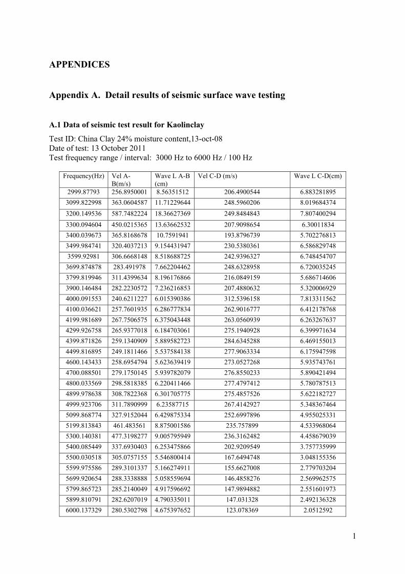
1
APPENDICES
Appendix A. Detail results of seismic surface wave testing
A.1 Data of seismic test result for Kaolinclay
Test ID: China Clay 24% moisture content,13-oct-08 Date of test: 13 October 2011 Test frequency range / interval: 3000 Hz to 6000 Hz / 100 Hz
Frequency(Hz) Vel A-B(m/s)
Wave L A-B (cm)
Vel C-D (m/s) Wave L C-D(cm)
2999.87793 256.8950001 8.56351512 206.4900544 6.883281895
3099.822998 363.0604587 11.71229644 248.5960206 8.019684374
3200.149536 587.7482224 18.36627369 249.8484843 7.807400294
3300.094604 450.0215365 13.63662532 207.9098654 6.30011834
3400.039673 365.8168678 10.7591941 193.8796739 5.702276813
3499.984741 320.4037213 9.154431947 230.5380361 6.586829748
3599.92981 306.6668148 8.518688725 242.9396327 6.748454707
3699.874878 283.491978 7.662204462 248.6328958 6.720035245
3799.819946 311.4399634 8.196176866 216.0849159 5.686714606
3900.146484 282.2230572 7.236216853 207.4880632 5.320006929
4000.091553 240.6211227 6.015390386 312.5396158 7.813311562
4100.036621 257.7601935 6.286777834 262.9016777 6.412178768
4199.981689 267.7506575 6.375043448 263.0560939 6.263267637
4299.926758 265.9377018 6.184703061 275.1940928 6.399971634
4399.871826 259.1340909 5.889582723 284.6345288 6.469155013
4499.816895 249.1811466 5.537584138 277.9063334 6.175947598
4600.143433 258.6954794 5.623639419 273.0527268 5.935743761
4700.088501 279.1750145 5.939782079 276.8550233 5.890421494
4800.033569 298.5818385 6.220411466 277.4797412 5.780787513
4899.978638 308.7822368 6.301705775 275.4857526 5.622182727
4999.923706 311.7890999 6.23587715 267.4142927 5.348367464
5099.868774 327.9152044 6.429875334 252.6997896 4.955025331
5199.813843 461.483561 8.875001586 235.757899 4.533968064
5300.140381 477.3198277 9.005795949 236.3162482 4.458679039
5400.085449 337.6930403 6.253475866 202.9209549 3.757735999
5500.030518 305.0757155 5.546800414 167.6494748 3.048155356
5599.975586 289.3101337 5.166274911 155.6627008 2.779703204
5699.920654 288.3338888 5.058559694 146.4858276 2.569962575
5799.865723 285.2140049 4.917596692 147.9894882 2.551601973
5899.810791 282.6207019 4.790335011 147.031328 2.492136328
6000.137329 280.5302798 4.675397652 123.078369 2.0512592
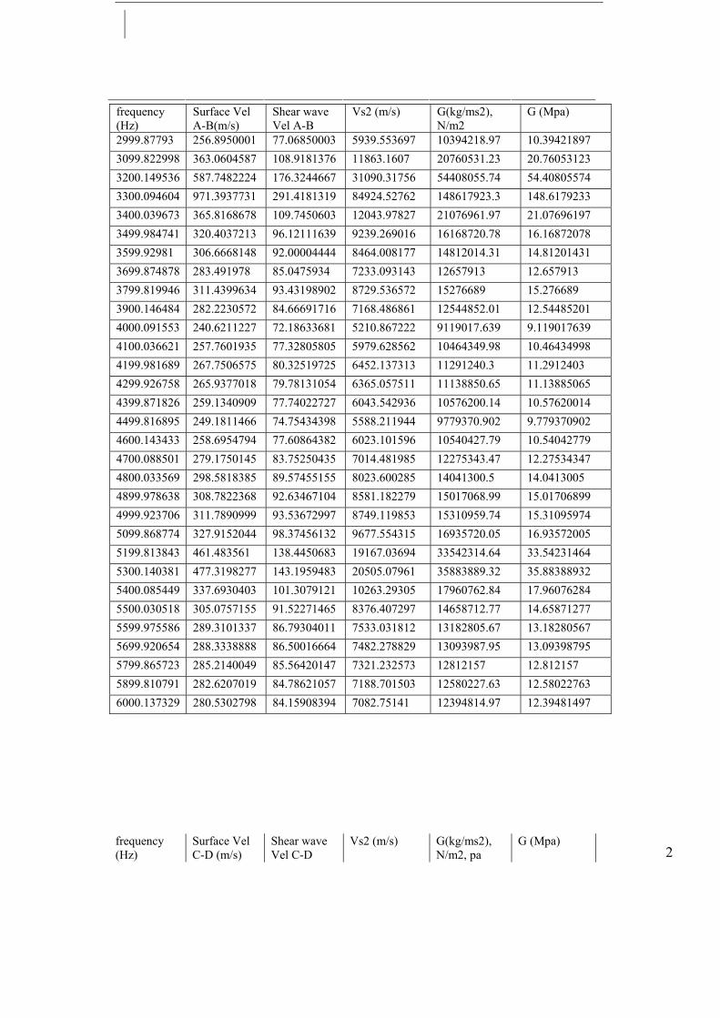
frequency (Hz)
Surface Vel A-B(m/s)
Shear wave Vel A-B
Vs2 (m/s) G(kg/ms2), N/m2
G (Mpa)
2999.87793 256.8950001 77.06850003 5939.553697 10394218.97 10.39421897
3099.822998 363.0604587 108.9181376 11863.1607 20760531.23 20.76053123
3200.149536 587.7482224 176.3244667 31090.31756 54408055.74 54.40805574
3300.094604 971.3937731 291.4181319 84924.52762 148617923.3 148.6179233
3400.039673 365.8168678 109.7450603 12043.97827 21076961.97 21.07696197
3499.984741 320.4037213 96.12111639 9239.269016 16168720.78 16.16872078
3599.92981 306.6668148 92.00004444 8464.008177 14812014.31 14.81201431
3699.874878 283.491978 85.0475934 7233.093143 12657913 12.657913
3799.819946 311.4399634 93.43198902 8729.536572 15276689 15.276689
3900.146484 282.2230572 84.66691716 7168.486861 12544852.01 12.54485201
4000.091553 240.6211227 72.18633681 5210.867222 9119017.639 9.119017639
4100.036621 257.7601935 77.32805805 5979.628562 10464349.98 10.46434998
4199.981689 267.7506575 80.32519725 6452.137313 11291240.3 11.2912403
4299.926758 265.9377018 79.78131054 6365.057511 11138850.65 11.13885065
4399.871826 259.1340909 77.74022727 6043.542936 10576200.14 10.57620014
4499.816895 249.1811466 74.75434398 5588.211944 9779370.902 9.779370902
4600.143433 258.6954794 77.60864382 6023.101596 10540427.79 10.54042779
4700.088501 279.1750145 83.75250435 7014.481985 12275343.47 12.27534347
4800.033569 298.5818385 89.57455155 8023.600285 14041300.5 14.0413005
4899.978638 308.7822368 92.63467104 8581.182279 15017068.99 15.01706899
4999.923706 311.7890999 93.53672997 8749.119853 15310959.74 15.31095974
5099.868774 327.9152044 98.37456132 9677.554315 16935720.05 16.93572005
5199.813843 461.483561 138.4450683 19167.03694 33542314.64 33.54231464
5300.140381 477.3198277 143.1959483 20505.07961 35883889.32 35.88388932
5400.085449 337.6930403 101.3079121 10263.29305 17960762.84 17.96076284
5500.030518 305.0757155 91.52271465 8376.407297 14658712.77 14.65871277
5599.975586 289.3101337 86.79304011 7533.031812 13182805.67 13.18280567
5699.920654 288.3338888 86.50016664 7482.278829 13093987.95 13.09398795
5799.865723 285.2140049 85.56420147 7321.232573 12812157 12.812157
5899.810791 282.6207019 84.78621057 7188.701503 12580227.63 12.58022763
6000.137329 280.5302798 84.15908394 7082.75141 12394814.97 12.39481497
2
frequency (Hz)
Surface Vel C-D (m/s)
Shear wave Vel C-D
Vs2 (m/s) G(kg/ms2), N/m2, pa
G (Mpa)

3
(m/s)
2999.87793 206.4900544 61.94701632 3837.432831 6715507.454 6.715507454
3099.822998 248.5960206 74.57880618 5561.998331 9733497.08 9.73349708
3200.149536 249.8484843 74.95454529 5618.18386 9831821.754 9.831821754
3300.094604 207.9098654 62.37295962 3890.386092 6808175.661 6.808175661
3400.039673 193.8796739 58.16390217 3383.039516 5920319.152 5.920319152
3499.984741 230.5380361 69.16141083 4783.300748 8370776.309 8.370776309
3599.92981 242.9396327 72.88188981 5311.769862 9295597.259 9.295597259
3699.874878 248.6328958 74.58986874 5563.648519 9736384.908 9.736384908
3799.819946 216.0849159 64.82547477 4202.342179 7354098.814 7.354098814
3900.146484 207.4880632 62.24641896 3874.616673 6780579.178 6.780579178
4000.091553 312.5396158 93.76188474 8791.29103 15384759.3 15.3847593
4100.036621 262.9016777 78.87050331 6220.556292 10885973.51 10.88597351
4199.981689 263.0560939 78.91682817 6227.865768 10898765.09 10.89876509
4299.926758 275.1940928 82.55822784 6815.860984 11927756.72 11.92775672
4399.871826 284.6345288 85.39035864 7291.513349 12760148.36 12.76014836
4499.816895 277.9063334 83.37190002 6950.873713 12164029 12.164029
4600.143433 273.0527268 81.91581804 6710.201245 11742852.18 11.74285218
4700.088501 276.8550233 83.05650699 6898.383353 12072170.87 12.07217087
4800.033569 277.4797412 83.24392236 6929.55061 12126713.57 12.12671357
4899.978638 275.4857526 82.64572578 6830.31599 11953052.98 11.95305298
4999.923706 267.4142927 80.22428781 6435.936355 11262888.62 11.26288862
5099.868774 252.6997896 75.809936 5747.14653 10057506.43 10.05750643
5199.813843 235.757899 70.7273697 5002.360825 8754131.443 8.754131443
5300.140381 236.3162482 70.89487446 5026.083225 8795645.643 8.795645643
5400.085449 202.9209549 60.87628647 3705.922254 6485363.945 6.485363945
5500.030518 167.6494748 50.29484244 2529.571176 4426749.558 4.426749558
5599.975586 155.6627008 46.69881024 2180.778878 3816363.036 3.816363036
5699.920654 146.4858276 43.94574828 1931.228792 3379650.386 3.379650386
5799.865723 147.9894882 44.39684646 1971.079976 3449389.957 3.449389957
5899.810791 147.031328 44.1093984 1945.639027 3404868.298 3.404868298
6000.137329 123.078369 36.9235107 1363.345642 2385854.874 2.385854874
Test ID: China Clay 28% moisture content, 06-sep-03 Date of test: 06 September 2011
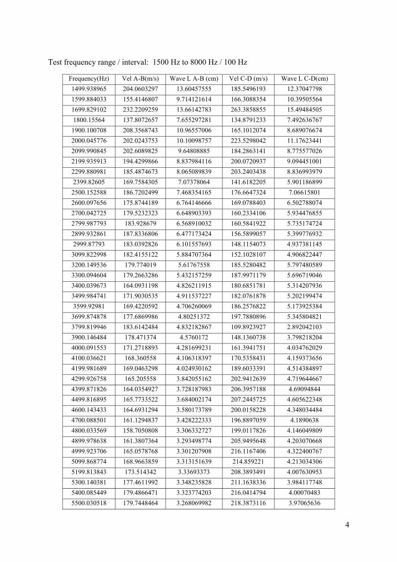
4
Test frequency range / interval: 1500 Hz to 8000 Hz / 100 Hz
Frequency(Hz) Vel A-B(m/s) Wave L A-B (cm) Vel C-D (m/s) Wave L C-D(cm)
1499.938965 204.0603297 13.60457555 185.5496193 12.37047798
1599.884033 155.4146807 9.714121614 166.3088354 10.39505564
1699.829102 232.2209259 13.66142783 263.3858855 15.49484505
1800.15564 137.8072657 7.655297281 134.8791233 7.492636767
1900.100708 208.3568743 10.96557006 165.1012074 8.689076674
2000.045776 202.0243753 10.10098757 223.5298042 11.17623441
2099.990845 202.6089825 9.64808885 184.2863141 8.775577026
2199.935913 194.4299866 8.837984116 200.0720937 9.094451001
2299.880981 185.4874673 8.065089839 203.2403438 8.836993979
2399.82605 169.7584305 7.07378064 141.6182205 5.901186899
2500.152588 186.7202499 7.468354165 176.6647324 7.06615801
2600.097656 175.8744189 6.764146666 169.0788403 6.502788074
2700.042725 179.5232323 6.648903393 160.2334106 5.934476855
2799.987793 183.928679 6.568910032 160.5841922 5.735174724
2899.932861 187.8336806 6.477173424 156.5899057 5.399776932
2999.87793 183.0392826 6.101557693 148.1154073 4.937381145
3099.822998 182.4155122 5.884707364 152.1028107 4.906822447
3200.149536 179.774019 5.61767558 185.5280482 5.797480589
3300.094604 179.2663286 5.432157259 187.9971179 5.696719046
3400.039673 164.0931198 4.826211915 180.6851781 5.314207936
3499.984741 171.9030535 4.911537227 182.0761878 5.202199474
3599.92981 169.4220592 4.706260069 186.2576822 5.173925384
3699.874878 177.6869986 4.80251372 197.7880896 5.345804821
3799.819946 183.6142484 4.832182867 109.8923927 2.892042103
3900.146484 178.471374 4.5760172 148.1360738 3.798218204
4000.091553 171.2718893 4.281699231 161.3941751 4.034762029
4100.036621 168.360558 4.106318397 170.5358431 4.159373656
4199.981689 169.0463298 4.024930162 189.6033391 4.514384897
4299.926758 165.205558 3.842055162 202.9412639 4.719644667
4399.871826 164.0354927 3.728187983 206.3957188 4.69094844
4499.816895 165.7733522 3.684002174 207.2445725 4.605622348
4600.143433 164.6931294 3.580173789 200.0158228 4.348034484
4700.088501 161.1294837 3.428222333 196.8897059 4.1890638
4800.033569 158.7050808 3.306332727 199.0117826 4.146049809
4899.978638 161.3807364 3.293498774 205.9495648 4.203070668
4999.923706 165.0578768 3.301207908 216.1167406 4.322400767
5099.868774 168.9663859 3.313151639 214.859221 4.213034306
5199.813843 173.514342 3.33693373 208.3893491 4.007630953
5300.140381 177.4611992 3.348235828 211.1638336 3.984117748
5400.085449 179.4866471 3.323774203 216.0414794 4.00070483
5500.030518 179.7448464 3.268069982 218.3873116 3.97065636
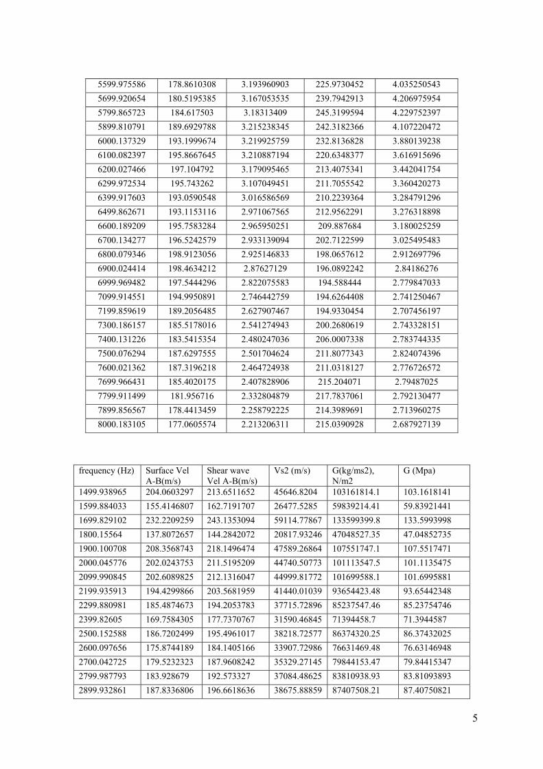
5
5599.975586 178.8610308 3.193960903 225.9730452 4.035250543
5699.920654 180.5195385 3.167053535 239.7942913 4.206975954
5799.865723 184.617503 3.18313409 245.3199594 4.229752397
5899.810791 189.6929788 3.215238345 242.3182366 4.107220472
6000.137329 193.1999674 3.219925759 232.8136828 3.880139238
6100.082397 195.8667645 3.210887194 220.6348377 3.616915696
6200.027466 197.104792 3.179095465 213.4075341 3.442041754
6299.972534 195.743262 3.107049451 211.7055542 3.360420273
6399.917603 193.0590548 3.016586569 210.2239364 3.284791296
6499.862671 193.1153116 2.971067565 212.9562291 3.276318898
6600.189209 195.7583284 2.965950251 209.887684 3.180025259
6700.134277 196.5242579 2.933139094 202.7122599 3.025495483
6800.079346 198.9123056 2.925146833 198.0657612 2.912697796
6900.024414 198.4634212 2.87627129 196.0892242 2.84186276
6999.969482 197.5444296 2.822075583 194.588444 2.779847033
7099.914551 194.9950891 2.746442759 194.6264408 2.741250467
7199.859619 189.2056485 2.627907467 194.9330454 2.707456197
7300.186157 185.5178016 2.541274943 200.2680619 2.743328151
7400.131226 183.5415354 2.480247036 206.0007338 2.783744335
7500.076294 187.6297555 2.501704624 211.8077343 2.824074396
7600.021362 187.3196218 2.464724938 211.0318127 2.776726572
7699.966431 185.4020175 2.407828906 215.204071 2.79487025
7799.911499 181.956716 2.332804879 217.7837061 2.792130477
7899.856567 178.4413459 2.258792225 214.3989691 2.713960275
8000.183105 177.0605574 2.213206311 215.0390928 2.687927139
frequency (Hz) Surface Vel A-B(m/s)
Shear wave Vel A-B(m/s)
Vs2 (m/s) G(kg/ms2), N/m2
G (Mpa)
1499.938965 204.0603297 213.6511652 45646.8204 103161814.1 103.1618141
1599.884033 155.4146807 162.7191707 26477.5285 59839214.41 59.83921441
1699.829102 232.2209259 243.1353094 59114.77867 133599399.8 133.5993998
1800.15564 137.8072657 144.2842072 20817.93246 47048527.35 47.04852735
1900.100708 208.3568743 218.1496474 47589.26864 107551747.1 107.5517471
2000.045776 202.0243753 211.5195209 44740.50773 101113547.5 101.1135475
2099.990845 202.6089825 212.1316047 44999.81772 101699588.1 101.6995881
2199.935913 194.4299866 203.5681959 41440.01039 93654423.48 93.65442348
2299.880981 185.4874673 194.2053783 37715.72896 85237547.46 85.23754746
2399.82605 169.7584305 177.7370767 31590.46845 71394458.7 71.3944587
2500.152588 186.7202499 195.4961017 38218.72577 86374320.25 86.37432025
2600.097656 175.8744189 184.1405166 33907.72986 76631469.48 76.63146948
2700.042725 179.5232323 187.9608242 35329.27145 79844153.47 79.84415347
2799.987793 183.928679 192.573327 37084.48625 83810938.93 83.81093893
2899.932861 187.8336806 196.6618636 38675.88859 87407508.21 87.40750821
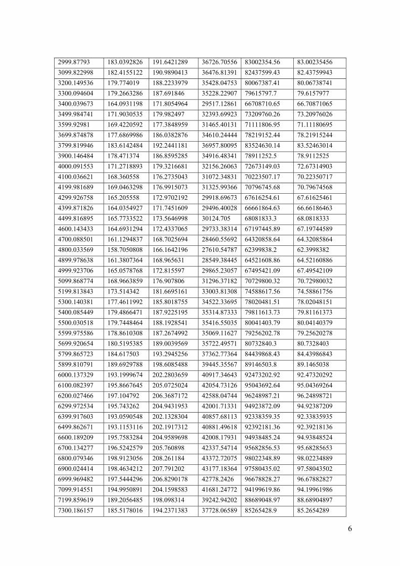
6
2999.87793 183.0392826 191.6421289 36726.70556 83002354.56 83.00235456
3099.822998 182.4155122 190.9890413 36476.81391 82437599.43 82.43759943
3200.149536 179.774019 188.2233979 35428.04753 80067387.41 80.06738741
3300.094604 179.2663286 187.691846 35228.22907 79615797.7 79.6157977
3400.039673 164.0931198 171.8054964 29517.12861 66708710.65 66.70871065
3499.984741 171.9030535 179.982497 32393.69923 73209760.26 73.20976026
3599.92981 169.4220592 177.3848959 31465.40131 71111806.95 71.11180695
3699.874878 177.6869986 186.0382876 34610.24444 78219152.44 78.21915244
3799.819946 183.6142484 192.2441181 36957.80095 83524630.14 83.52463014
3900.146484 178.471374 186.8595285 34916.48341 78911252.5 78.9112525
4000.091553 171.2718893 179.3216681 32156.26063 72673149.03 72.67314903
4100.036621 168.360558 176.2735043 31072.34831 70223507.17 70.22350717
4199.981689 169.0463298 176.9915073 31325.99366 70796745.68 70.79674568
4299.926758 165.205558 172.9702192 29918.69673 67616254.61 67.61625461
4399.871826 164.0354927 171.7451609 29496.40028 66661864.63 66.66186463
4499.816895 165.7733522 173.5646998 30124.705 68081833.3 68.0818333
4600.143433 164.6931294 172.4337065 29733.38314 67197445.89 67.19744589
4700.088501 161.1294837 168.7025694 28460.55692 64320858.64 64.32085864
4800.033569 158.7050808 166.1642196 27610.54787 62399838.2 62.3998382
4899.978638 161.3807364 168.965631 28549.38445 64521608.86 64.52160886
4999.923706 165.0578768 172.815597 29865.23057 67495421.09 67.49542109
5099.868774 168.9663859 176.907806 31296.37182 70729800.32 70.72980032
5199.813843 173.514342 181.6695161 33003.81308 74588617.56 74.58861756
5300.140381 177.4611992 185.8018755 34522.33695 78020481.51 78.02048151
5400.085449 179.4866471 187.9225195 35314.87333 79811613.73 79.81161373
5500.030518 179.7448464 188.1928541 35416.55035 80041403.79 80.04140379
5599.975586 178.8610308 187.2674992 35069.11627 79256202.78 79.25620278
5699.920654 180.5195385 189.0039569 35722.49571 80732840.3 80.7328403
5799.865723 184.617503 193.2945256 37362.77364 84439868.43 84.43986843
5899.810791 189.6929788 198.6085488 39445.35567 89146503.8 89.1465038
6000.137329 193.1999674 202.2803659 40917.34643 92473202.92 92.47320292
6100.082397 195.8667645 205.0725024 42054.73126 95043692.64 95.04369264
6200.027466 197.104792 206.3687172 42588.04744 96248987.21 96.24898721
6299.972534 195.743262 204.9431953 42001.71331 94923872.09 94.92387209
6399.917603 193.0590548 202.1328304 40857.68113 92338359.35 92.33835935
6499.862671 193.1153116 202.1917312 40881.49618 92392181.36 92.39218136
6600.189209 195.7583284 204.9589698 42008.17931 94938485.24 94.93848524
6700.134277 196.5242579 205.760898 42337.54714 95682856.53 95.68285653
6800.079346 198.9123056 208.261184 43372.72075 98022348.89 98.02234889
6900.024414 198.4634212 207.791202 43177.18364 97580435.02 97.58043502
6999.969482 197.5444296 206.8290178 42778.2426 96678828.27 96.67882827
7099.914551 194.9950891 204.1598583 41681.24772 94199619.86 94.19961986
7199.859619 189.2056485 198.098314 39242.94202 88689048.97 88.68904897
7300.186157 185.5178016 194.2371383 37728.06589 85265428.9 85.2654289
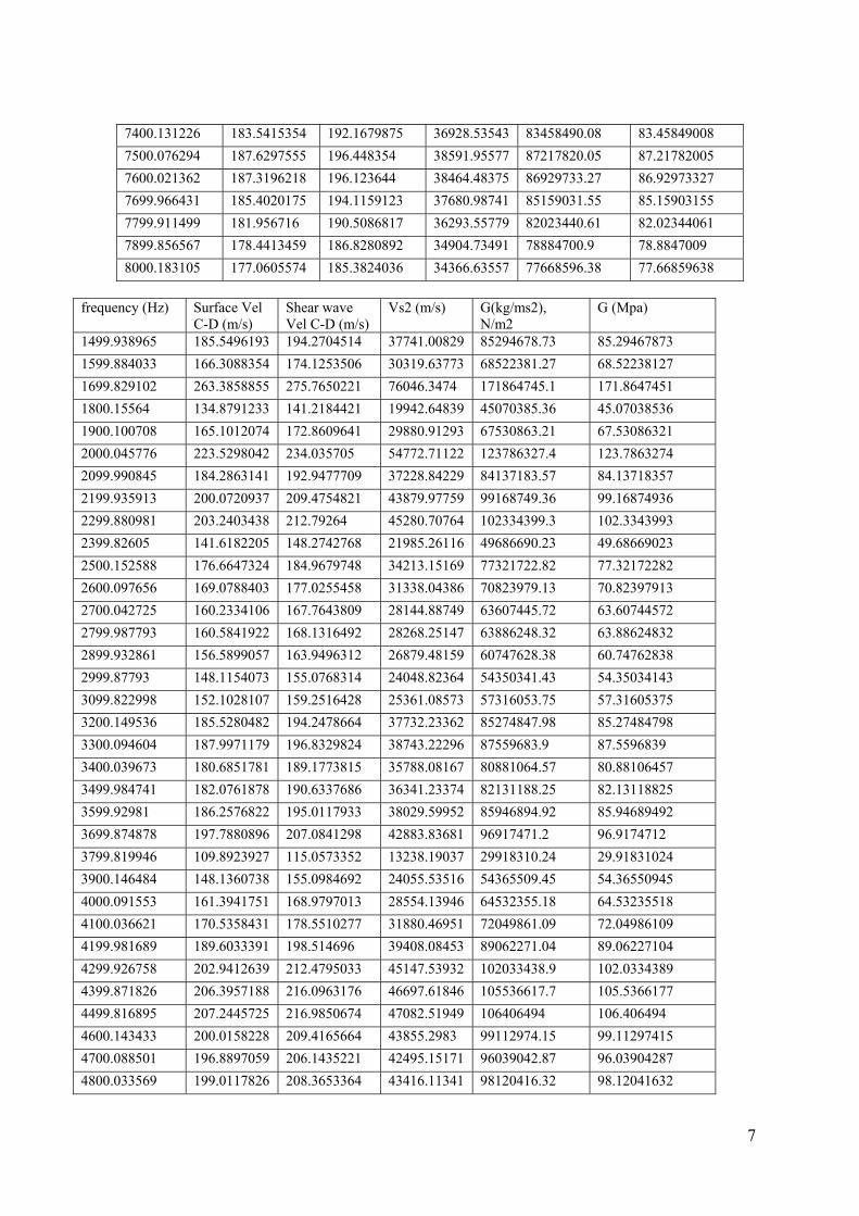
7
7400.131226 183.5415354 192.1679875 36928.53543 83458490.08 83.45849008
7500.076294 187.6297555 196.448354 38591.95577 87217820.05 87.21782005
7600.021362 187.3196218 196.123644 38464.48375 86929733.27 86.92973327
7699.966431 185.4020175 194.1159123 37680.98741 85159031.55 85.15903155
7799.911499 181.956716 190.5086817 36293.55779 82023440.61 82.02344061
7899.856567 178.4413459 186.8280892 34904.73491 78884700.9 78.8847009
8000.183105 177.0605574 185.3824036 34366.63557 77668596.38 77.66859638
frequency (Hz) Surface Vel
C-D (m/s) Shear wave Vel C-D (m/s)
Vs2 (m/s) G(kg/ms2), N/m2
G (Mpa)
1499.938965 185.5496193 194.2704514 37741.00829 85294678.73 85.29467873
1599.884033 166.3088354 174.1253506 30319.63773 68522381.27 68.52238127
1699.829102 263.3858855 275.7650221 76046.3474 171864745.1 171.8647451
1800.15564 134.8791233 141.2184421 19942.64839 45070385.36 45.07038536
1900.100708 165.1012074 172.8609641 29880.91293 67530863.21 67.53086321
2000.045776 223.5298042 234.035705 54772.71122 123786327.4 123.7863274
2099.990845 184.2863141 192.9477709 37228.84229 84137183.57 84.13718357
2199.935913 200.0720937 209.4754821 43879.97759 99168749.36 99.16874936
2299.880981 203.2403438 212.79264 45280.70764 102334399.3 102.3343993
2399.82605 141.6182205 148.2742768 21985.26116 49686690.23 49.68669023
2500.152588 176.6647324 184.9679748 34213.15169 77321722.82 77.32172282
2600.097656 169.0788403 177.0255458 31338.04386 70823979.13 70.82397913
2700.042725 160.2334106 167.7643809 28144.88749 63607445.72 63.60744572
2799.987793 160.5841922 168.1316492 28268.25147 63886248.32 63.88624832
2899.932861 156.5899057 163.9496312 26879.48159 60747628.38 60.74762838
2999.87793 148.1154073 155.0768314 24048.82364 54350341.43 54.35034143
3099.822998 152.1028107 159.2516428 25361.08573 57316053.75 57.31605375
3200.149536 185.5280482 194.2478664 37732.23362 85274847.98 85.27484798
3300.094604 187.9971179 196.8329824 38743.22296 87559683.9 87.5596839
3400.039673 180.6851781 189.1773815 35788.08167 80881064.57 80.88106457
3499.984741 182.0761878 190.6337686 36341.23374 82131188.25 82.13118825
3599.92981 186.2576822 195.0117933 38029.59952 85946894.92 85.94689492
3699.874878 197.7880896 207.0841298 42883.83681 96917471.2 96.9174712
3799.819946 109.8923927 115.0573352 13238.19037 29918310.24 29.91831024
3900.146484 148.1360738 155.0984692 24055.53516 54365509.45 54.36550945
4000.091553 161.3941751 168.9797013 28554.13946 64532355.18 64.53235518
4100.036621 170.5358431 178.5510277 31880.46951 72049861.09 72.04986109
4199.981689 189.6033391 198.514696 39408.08453 89062271.04 89.06227104
4299.926758 202.9412639 212.4795033 45147.53932 102033438.9 102.0334389
4399.871826 206.3957188 216.0963176 46697.61846 105536617.7 105.5366177
4499.816895 207.2445725 216.9850674 47082.51949 106406494 106.406494
4600.143433 200.0158228 209.4165664 43855.2983 99112974.15 99.11297415
4700.088501 196.8897059 206.1435221 42495.15171 96039042.87 96.03904287
4800.033569 199.0117826 208.3653364 43416.11341 98120416.32 98.12041632
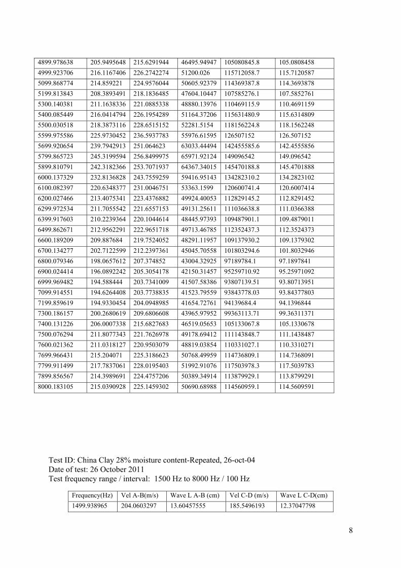
8
4899.978638 205.9495648 215.6291944 46495.94947 105080845.8 105.0808458
4999.923706 216.1167406 226.2742274 51200.026 115712058.7 115.7120587
5099.868774 214.859221 224.9576044 50605.92379 114369387.8 114.3693878
5199.813843 208.3893491 218.1836485 47604.10447 107585276.1 107.5852761
5300.140381 211.1638336 221.0885338 48880.13976 110469115.9 110.4691159
5400.085449 216.0414794 226.1954289 51164.37206 115631480.9 115.6314809
5500.030518 218.3873116 228.6515152 52281.5154 118156224.8 118.1562248
5599.975586 225.9730452 236.5937783 55976.61595 126507152 126.507152
5699.920654 239.7942913 251.064623 63033.44494 142455585.6 142.4555856
5799.865723 245.3199594 256.8499975 65971.92124 149096542 149.096542
5899.810791 242.3182366 253.7071937 64367.34015 145470188.8 145.4701888
6000.137329 232.8136828 243.7559259 59416.95143 134282310.2 134.2823102
6100.082397 220.6348377 231.0046751 53363.1599 120600741.4 120.6007414
6200.027466 213.4075341 223.4376882 49924.40053 112829145.2 112.8291452
6299.972534 211.7055542 221.6557153 49131.25611 111036638.8 111.0366388
6399.917603 210.2239364 220.1044614 48445.97393 109487901.1 109.4879011
6499.862671 212.9562291 222.9651718 49713.46785 112352437.3 112.3524373
6600.189209 209.887684 219.7524052 48291.11957 109137930.2 109.1379302
6700.134277 202.7122599 212.2397361 45045.70558 101803294.6 101.8032946
6800.079346 198.0657612 207.374852 43004.32925 97189784.1 97.1897841
6900.024414 196.0892242 205.3054178 42150.31457 95259710.92 95.25971092
6999.969482 194.588444 203.7341009 41507.58386 93807139.51 93.80713951
7099.914551 194.6264408 203.7738835 41523.79559 93843778.03 93.84377803
7199.859619 194.9330454 204.0948985 41654.72761 94139684.4 94.1396844
7300.186157 200.2680619 209.6806608 43965.97952 99363113.71 99.36311371
7400.131226 206.0007338 215.6827683 46519.05653 105133067.8 105.1330678
7500.076294 211.8077343 221.7626978 49178.69412 111143848.7 111.1438487
7600.021362 211.0318127 220.9503079 48819.03854 110331027.1 110.3310271
7699.966431 215.204071 225.3186623 50768.49959 114736809.1 114.7368091
7799.911499 217.7837061 228.0195403 51992.91076 117503978.3 117.5039783
7899.856567 214.3989691 224.4757206 50389.34914 113879929.1 113.8799291
8000.183105 215.0390928 225.1459302 50690.68988 114560959.1 114.5609591
Test ID: China Clay 28% moisture content-Repeated, 26-oct-04 Date of test: 26 October 2011 Test frequency range / interval: 1500 Hz to 8000 Hz / 100 Hz
Frequency(Hz) Vel A-B(m/s) Wave L A-B (cm) Vel C-D (m/s) Wave L C-D(cm)
1499.938965 204.0603297 13.60457555 185.5496193 12.37047798

9
1599.884033 155.4146807 9.714121614 166.3088354 10.39505564
1699.829102 232.2209259 13.66142783 263.3858855 15.49484505
1800.15564 137.8072657 7.655297281 134.8791233 7.492636767
1900.100708 208.3568743 10.96557006 165.1012074 8.689076674
2000.045776 202.0243753 10.10098757 223.5298042 11.17623441
2099.990845 202.6089825 9.64808885 184.2863141 8.775577026
2199.935913 194.4299866 8.837984116 200.0720937 9.094451001
2299.880981 185.4874673 8.065089839 203.2403438 8.836993979
2399.82605 169.7584305 7.07378064 141.6182205 5.901186899
2500.152588 186.7202499 7.468354165 176.6647324 7.06615801
2600.097656 175.8744189 6.764146666 169.0788403 6.502788074
2700.042725 179.5232323 6.648903393 160.2334106 5.934476855
2799.987793 183.928679 6.568910032 160.5841922 5.735174724
2899.932861 187.8336806 6.477173424 156.5899057 5.399776932
2999.87793 183.0392826 6.101557693 148.1154073 4.937381145
3099.822998 182.4155122 5.884707364 152.1028107 4.906822447
3200.149536 179.774019 5.61767558 185.5280482 5.797480589
3300.094604 179.2663286 5.432157259 187.9971179 5.696719046
3400.039673 164.0931198 4.826211915 180.6851781 5.314207936
3499.984741 171.9030535 4.911537227 182.0761878 5.202199474
3599.92981 169.4220592 4.706260069 186.2576822 5.173925384
3699.874878 177.6869986 4.80251372 197.7880896 5.345804821
3799.819946 183.6142484 4.832182867 109.8923927 2.892042103
3900.146484 178.471374 4.5760172 148.1360738 3.798218204
4000.091553 171.2718893 4.281699231 161.3941751 4.034762029
4100.036621 168.360558 4.106318397 170.5358431 4.159373656
4199.981689 169.0463298 4.024930162 189.6033391 4.514384897
4299.926758 165.205558 3.842055162 202.9412639 4.719644667
4399.871826 164.0354927 3.728187983 206.3957188 4.69094844
4499.816895 165.7733522 3.684002174 207.2445725 4.605622348
4600.143433 164.6931294 3.580173789 200.0158228 4.348034484
4700.088501 161.1294837 3.428222333 196.8897059 4.1890638
4800.033569 158.7050808 3.306332727 199.0117826 4.146049809
4899.978638 161.3807364 3.293498774 205.9495648 4.203070668
4999.923706 165.0578768 3.301207908 216.1167406 4.322400767
5099.868774 168.9663859 3.313151639 214.859221 4.213034306
5199.813843 173.514342 3.33693373 208.3893491 4.007630953
5300.140381 177.4611992 3.348235828 211.1638336 3.984117748
5400.085449 179.4866471 3.323774203 216.0414794 4.00070483
5500.030518 179.7448464 3.268069982 218.3873116 3.97065636
5599.975586 178.8610308 3.193960903 225.9730452 4.035250543
5699.920654 180.5195385 3.167053535 239.7942913 4.206975954
5799.865723 184.617503 3.18313409 245.3199594 4.229752397
5899.810791 189.6929788 3.215238345 242.3182366 4.107220472

10
6000.137329 193.1999674 3.219925759 232.8136828 3.880139238
6100.082397 195.8667645 3.210887194 220.6348377 3.616915696
6200.027466 197.104792 3.179095465 213.4075341 3.442041754
6299.972534 195.743262 3.107049451 211.7055542 3.360420273
6399.917603 193.0590548 3.016586569 210.2239364 3.284791296
6499.862671 193.1153116 2.971067565 212.9562291 3.276318898
6600.189209 195.7583284 2.965950251 209.887684 3.180025259
6700.134277 196.5242579 2.933139094 202.7122599 3.025495483
6800.079346 198.9123056 2.925146833 198.0657612 2.912697796
6900.024414 198.4634212 2.87627129 196.0892242 2.84186276
6999.969482 197.5444296 2.822075583 194.588444 2.779847033
7099.914551 194.9950891 2.746442759 194.6264408 2.741250467
7199.859619 189.2056485 2.627907467 194.9330454 2.707456197
7300.186157 185.5178016 2.541274943 200.2680619 2.743328151
7400.131226 183.5415354 2.480247036 206.0007338 2.783744335
7500.076294 187.6297555 2.501704624 211.8077343 2.824074396
7600.021362 187.3196218 2.464724938 211.0318127 2.776726572
7699.966431 185.4020175 2.407828906 215.204071 2.79487025
7799.911499 181.956716 2.332804879 217.7837061 2.792130477
7899.856567 178.4413459 2.258792225 214.3989691 2.713960275
8000.183105 177.0605574 2.213206311 215.0390928 2.687927139
frequency (Hz)
Surface Vel A-B (m/s)
Shear wave Vel A-B (m/s)
Vs2 (m/s) G(kg/ms2), N/m2
G (Mpa)
1499.938965 204.0603297 213.6511652 45646.8204 103161814.1 103.1618141
1599.884033 155.4146807 162.7191707 26477.5285 59839214.41 59.83921441
1699.829102 232.2209259 243.1353094 59114.77867 133599399.8 133.5993998
1800.15564 137.8072657 144.2842072 20817.93246 47048527.35 47.04852735
1900.100708 208.3568743 218.1496474 47589.26864 107551747.1 107.5517471
2000.045776 202.0243753 211.5195209 44740.50773 101113547.5 101.1135475
2099.990845 202.6089825 212.1316047 44999.81772 101699588.1 101.6995881
2199.935913 194.4299866 203.5681959 41440.01039 93654423.48 93.65442348
2299.880981 185.4874673 194.2053783 37715.72896 85237547.46 85.23754746
2399.82605 169.7584305 177.7370767 31590.46845 71394458.7 71.3944587
2500.152588 186.7202499 195.4961017 38218.72577 86374320.25 86.37432025
2600.097656 175.8744189 184.1405166 33907.72986 76631469.48 76.63146948
2700.042725 179.5232323 187.9608242 35329.27145 79844153.47 79.84415347
2799.987793 183.928679 192.573327 37084.48625 83810938.93 83.81093893
2899.932861 187.8336806 196.6618636 38675.88859 87407508.21 87.40750821
2999.87793 183.0392826 191.6421289 36726.70556 83002354.56 83.00235456
3099.822998 182.4155122 190.9890413 36476.81391 82437599.43 82.43759943
3200.149536 179.774019 188.2233979 35428.04753 80067387.41 80.06738741
3300.094604 179.2663286 187.691846 35228.22907 79615797.7 79.6157977
3400.039673 164.0931198 171.8054964 29517.12861 66708710.65 66.70871065
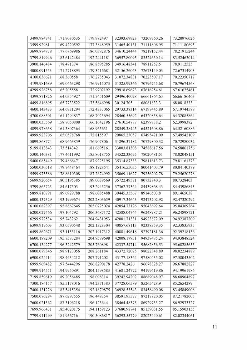
11
3499.984741 171.9030535 179.982497 32393.69923 73209760.26 73.20976026
3599.92981 169.4220592 177.3848959 31465.40131 71111806.95 71.11180695
3699.874878 177.6869986 186.0382876 34610.24444 78219152.44 78.21915244
3799.819946 183.6142484 192.2441181 36957.80095 83524630.14 83.52463014
3900.146484 178.471374 186.8595285 34916.48341 78911252.5 78.9112525
4000.091553 171.2718893 179.3216681 32156.26063 72673149.03 72.67314903
4100.036621 168.360558 176.2735043 31072.34831 70223507.17 70.22350717
4199.981689 169.0463298 176.9915073 31325.99366 70796745.68 70.79674568
4299.926758 165.205558 172.9702192 29918.69673 67616254.61 67.61625461
4399.871826 164.0354927 171.7451609 29496.40028 66661864.63 66.66186463
4499.816895 165.7733522 173.5646998 30124.705 68081833.3 68.0818333
4600.143433 164.6931294 172.4337065 29733.38314 67197445.89 67.19744589
4700.088501 161.1294837 168.7025694 28460.55692 64320858.64 64.32085864
4800.033569 158.7050808 166.1642196 27610.54787 62399838.2 62.3998382
4899.978638 161.3807364 168.965631 28549.38445 64521608.86 64.52160886
4999.923706 165.0578768 172.815597 29865.23057 67495421.09 67.49542109
5099.868774 168.9663859 176.907806 31296.37182 70729800.32 70.72980032
5199.813843 173.514342 181.6695161 33003.81308 74588617.56 74.58861756
5300.140381 177.4611992 185.8018755 34522.33695 78020481.51 78.02048151
5400.085449 179.4866471 187.9225195 35314.87333 79811613.73 79.81161373
5500.030518 179.7448464 188.1928541 35416.55035 80041403.79 80.04140379
5599.975586 178.8610308 187.2674992 35069.11627 79256202.78 79.25620278
5699.920654 180.5195385 189.0039569 35722.49571 80732840.3 80.7328403
5799.865723 184.617503 193.2945256 37362.77364 84439868.43 84.43986843
5899.810791 189.6929788 198.6085488 39445.35567 89146503.8 89.1465038
6000.137329 193.1999674 202.2803659 40917.34643 92473202.92 92.47320292
6100.082397 195.8667645 205.0725024 42054.73126 95043692.64 95.04369264
6200.027466 197.104792 206.3687172 42588.04744 96248987.21 96.24898721
6299.972534 195.743262 204.9431953 42001.71331 94923872.09 94.92387209
6399.917603 193.0590548 202.1328304 40857.68113 92338359.35 92.33835935
6499.862671 193.1153116 202.1917312 40881.49618 92392181.36 92.39218136
6600.189209 195.7583284 204.9589698 42008.17931 94938485.24 94.93848524
6700.134277 196.5242579 205.760898 42337.54714 95682856.53 95.68285653
6800.079346 198.9123056 208.261184 43372.72075 98022348.89 98.02234889
6900.024414 198.4634212 207.791202 43177.18364 97580435.02 97.58043502
6999.969482 197.5444296 206.8290178 42778.2426 96678828.27 96.67882827
7099.914551 194.9950891 204.1598583 41681.24772 94199619.86 94.19961986
7199.859619 189.2056485 198.098314 39242.94202 88689048.97 88.68904897
7300.186157 185.5178016 194.2371383 37728.06589 85265428.9 85.2654289
7400.131226 183.5415354 192.1679875 36928.53543 83458490.08 83.45849008
7500.076294 187.6297555 196.448354 38591.95577 87217820.05 87.21782005
7600.021362 187.3196218 196.123644 38464.48375 86929733.27 86.92973327
7699.966431 185.4020175 194.1159123 37680.98741 85159031.55 85.15903155
7799.911499 181.956716 190.5086817 36293.55779 82023440.61 82.02344061
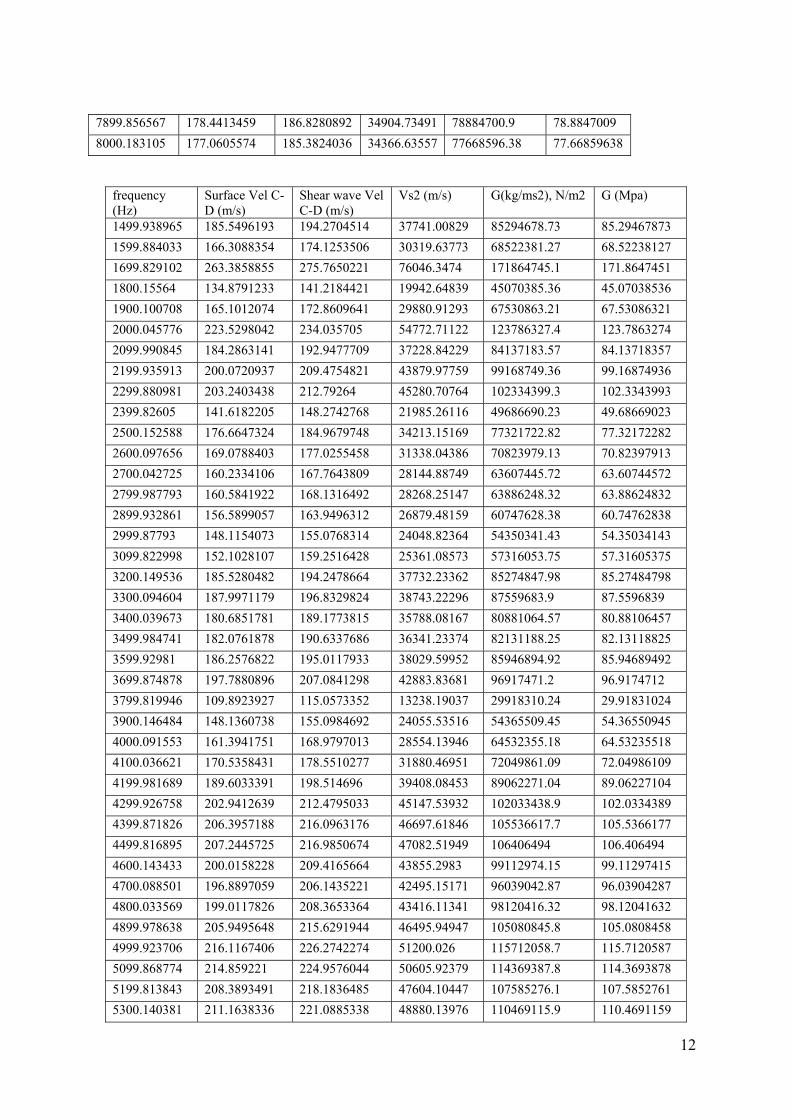
12
7899.856567 178.4413459 186.8280892 34904.73491 78884700.9 78.8847009
8000.183105 177.0605574 185.3824036 34366.63557 77668596.38 77.66859638
frequency (Hz)
Surface Vel C-D (m/s)
Shear wave Vel C-D (m/s)
Vs2 (m/s) G(kg/ms2), N/m2 G (Mpa)
1499.938965 185.5496193 194.2704514 37741.00829 85294678.73 85.29467873
1599.884033 166.3088354 174.1253506 30319.63773 68522381.27 68.52238127
1699.829102 263.3858855 275.7650221 76046.3474 171864745.1 171.8647451
1800.15564 134.8791233 141.2184421 19942.64839 45070385.36 45.07038536
1900.100708 165.1012074 172.8609641 29880.91293 67530863.21 67.53086321
2000.045776 223.5298042 234.035705 54772.71122 123786327.4 123.7863274
2099.990845 184.2863141 192.9477709 37228.84229 84137183.57 84.13718357
2199.935913 200.0720937 209.4754821 43879.97759 99168749.36 99.16874936
2299.880981 203.2403438 212.79264 45280.70764 102334399.3 102.3343993
2399.82605 141.6182205 148.2742768 21985.26116 49686690.23 49.68669023
2500.152588 176.6647324 184.9679748 34213.15169 77321722.82 77.32172282
2600.097656 169.0788403 177.0255458 31338.04386 70823979.13 70.82397913
2700.042725 160.2334106 167.7643809 28144.88749 63607445.72 63.60744572
2799.987793 160.5841922 168.1316492 28268.25147 63886248.32 63.88624832
2899.932861 156.5899057 163.9496312 26879.48159 60747628.38 60.74762838
2999.87793 148.1154073 155.0768314 24048.82364 54350341.43 54.35034143
3099.822998 152.1028107 159.2516428 25361.08573 57316053.75 57.31605375
3200.149536 185.5280482 194.2478664 37732.23362 85274847.98 85.27484798
3300.094604 187.9971179 196.8329824 38743.22296 87559683.9 87.5596839
3400.039673 180.6851781 189.1773815 35788.08167 80881064.57 80.88106457
3499.984741 182.0761878 190.6337686 36341.23374 82131188.25 82.13118825
3599.92981 186.2576822 195.0117933 38029.59952 85946894.92 85.94689492
3699.874878 197.7880896 207.0841298 42883.83681 96917471.2 96.9174712
3799.819946 109.8923927 115.0573352 13238.19037 29918310.24 29.91831024
3900.146484 148.1360738 155.0984692 24055.53516 54365509.45 54.36550945
4000.091553 161.3941751 168.9797013 28554.13946 64532355.18 64.53235518
4100.036621 170.5358431 178.5510277 31880.46951 72049861.09 72.04986109
4199.981689 189.6033391 198.514696 39408.08453 89062271.04 89.06227104
4299.926758 202.9412639 212.4795033 45147.53932 102033438.9 102.0334389
4399.871826 206.3957188 216.0963176 46697.61846 105536617.7 105.5366177
4499.816895 207.2445725 216.9850674 47082.51949 106406494 106.406494
4600.143433 200.0158228 209.4165664 43855.2983 99112974.15 99.11297415
4700.088501 196.8897059 206.1435221 42495.15171 96039042.87 96.03904287
4800.033569 199.0117826 208.3653364 43416.11341 98120416.32 98.12041632
4899.978638 205.9495648 215.6291944 46495.94947 105080845.8 105.0808458
4999.923706 216.1167406 226.2742274 51200.026 115712058.7 115.7120587
5099.868774 214.859221 224.9576044 50605.92379 114369387.8 114.3693878
5199.813843 208.3893491 218.1836485 47604.10447 107585276.1 107.5852761
5300.140381 211.1638336 221.0885338 48880.13976 110469115.9 110.4691159

13
5400.085449 216.0414794 226.1954289 51164.37206 115631480.9 115.6314809
5500.030518 218.3873116 228.6515152 52281.5154 118156224.8 118.1562248
5599.975586 225.9730452 236.5937783 55976.61595 126507152 126.507152
5699.920654 239.7942913 251.064623 63033.44494 142455585.6 142.4555856
5799.865723 245.3199594 256.8499975 65971.92124 149096542 149.096542
5899.810791 242.3182366 253.7071937 64367.34015 145470188.8 145.4701888
6000.137329 232.8136828 243.7559259 59416.95143 134282310.2 134.2823102
6100.082397 220.6348377 231.0046751 53363.1599 120600741.4 120.6007414
6200.027466 213.4075341 223.4376882 49924.40053 112829145.2 112.8291452
6299.972534 211.7055542 221.6557153 49131.25611 111036638.8 111.0366388
6399.917603 210.2239364 220.1044614 48445.97393 109487901.1 109.4879011
6499.862671 212.9562291 222.9651718 49713.46785 112352437.3 112.3524373
6600.189209 209.887684 219.7524052 48291.11957 109137930.2 109.1379302
6700.134277 202.7122599 212.2397361 45045.70558 101803294.6 101.8032946
6800.079346 198.0657612 207.374852 43004.32925 97189784.1 97.1897841
6900.024414 196.0892242 205.3054178 42150.31457 95259710.92 95.25971092
6999.969482 194.588444 203.7341009 41507.58386 93807139.51 93.80713951
7099.914551 194.6264408 203.7738835 41523.79559 93843778.03 93.84377803
7199.859619 194.9330454 204.0948985 41654.72761 94139684.4 94.1396844
7300.186157 200.2680619 209.6806608 43965.97952 99363113.71 99.36311371
7400.131226 206.0007338 215.6827683 46519.05653 105133067.8 105.1330678
7500.076294 211.8077343 221.7626978 49178.69412 111143848.7 111.1438487
7600.021362 211.0318127 220.9503079 48819.03854 110331027.1 110.3310271
7699.966431 215.204071 225.3186623 50768.49959 114736809.1 114.7368091
7799.911499 217.7837061 228.0195403 51992.91076 117503978.3 117.5039783
7899.856567 214.3989691 224.4757206 50389.34914 113879929.1 113.8799291
8000.183105 215.0390928 225.1459302 50690.68988 114560959.1 114.5609591
Test ID: China Clay 33% moisture content, 25-Agu-02 Date of test: 25 August 2011 Test frequency range / interval: 1000 Hz to 4000 Hz / 100 Hz
Frequency(Hz) Vel A-B(m/s) Wave L A-B (cm) Vel C-D (m/s) Wave L C-D(cm)
999.8321533 75.875766 7.588850363 81.0379549 8.105155913
1100.158691 70.8165959 6.436943728 69.6229592 6.328446957
1200.10376 66.447315 5.536797498 67.2536423 5.603985636
1300.048828 61.961702 4.766105757 62.5951987 4.814834439
1399.993896 70.9556478 5.068282654 62.112059 4.436594983
1499.938965 62.6387264 4.176085019 50.4430734 3.363008402
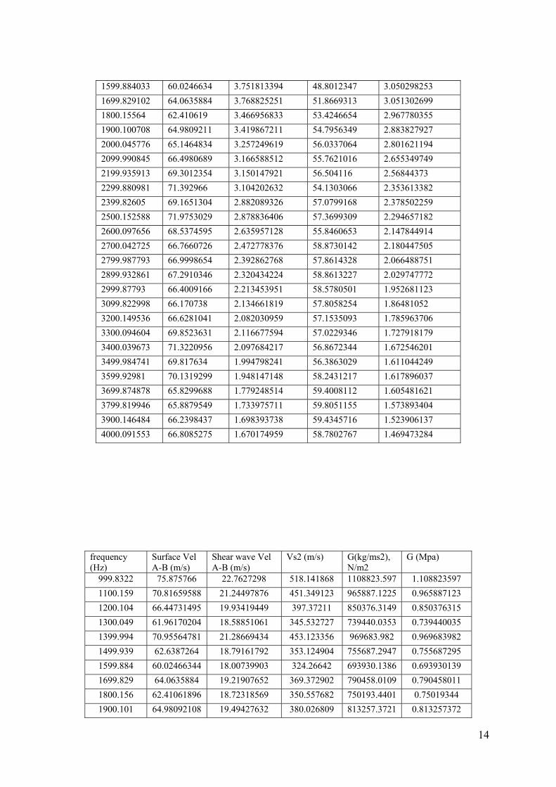
14
1599.884033 60.0246634 3.751813394 48.8012347 3.050298253
1699.829102 64.0635884 3.768825251 51.8669313 3.051302699
1800.15564 62.410619 3.466956833 53.4246654 2.967780355
1900.100708 64.9809211 3.419867211 54.7956349 2.883827927
2000.045776 65.1464834 3.257249619 56.0337064 2.801621194
2099.990845 66.4980689 3.166588512 55.7621016 2.655349749
2199.935913 69.3012354 3.150147921 56.504116 2.56844373
2299.880981 71.392966 3.104202632 54.1303066 2.353613382
2399.82605 69.1651304 2.882089326 57.0799168 2.378502259
2500.152588 71.9753029 2.878836406 57.3699309 2.294657182
2600.097656 68.5374595 2.635957128 55.8460653 2.147844914
2700.042725 66.7660726 2.472778376 58.8730142 2.180447505
2799.987793 66.9998654 2.392862768 57.8614328 2.066488751
2899.932861 67.2910346 2.320434224 58.8613227 2.029747772
2999.87793 66.4009166 2.213453951 58.5780501 1.952681123
3099.822998 66.170738 2.134661819 57.8058254 1.86481052
3200.149536 66.6281041 2.082030959 57.1535093 1.785963706
3300.094604 69.8523631 2.116677594 57.0229346 1.727918179
3400.039673 71.3220956 2.097684217 56.8672344 1.672546201
3499.984741 69.817634 1.994798241 56.3863029 1.611044249
3599.92981 70.1319299 1.948147148 58.2431217 1.617896037
3699.874878 65.8299688 1.779248514 59.4008112 1.605481621
3799.819946 65.8879549 1.733975711 59.8051155 1.573893404
3900.146484 66.2398437 1.698393738 59.4345716 1.523906137
4000.091553 66.8085275 1.670174959 58.7802767 1.469473284
frequency (Hz)
Surface Vel A-B (m/s)
Shear wave Vel A-B (m/s)
Vs2 (m/s) G(kg/ms2), N/m2
G (Mpa)
999.8322 75.875766 22.7627298 518.141868 1108823.597 1.108823597
1100.159 70.81659588 21.24497876 451.349123 965887.1225 0.965887123
1200.104 66.44731495 19.93419449 397.37211 850376.3149 0.850376315
1300.049 61.96170204 18.58851061 345.532727 739440.0353 0.739440035
1399.994 70.95564781 21.28669434 453.123356 969683.982 0.969683982
1499.939 62.6387264 18.79161792 353.124904 755687.2947 0.755687295
1599.884 60.02466344 18.00739903 324.26642 693930.1386 0.693930139
1699.829 64.0635884 19.21907652 369.372902 790458.0109 0.790458011
1800.156 62.41061896 18.72318569 350.557682 750193.4401 0.75019344
1900.101 64.98092108 19.49427632 380.026809 813257.3721 0.813257372
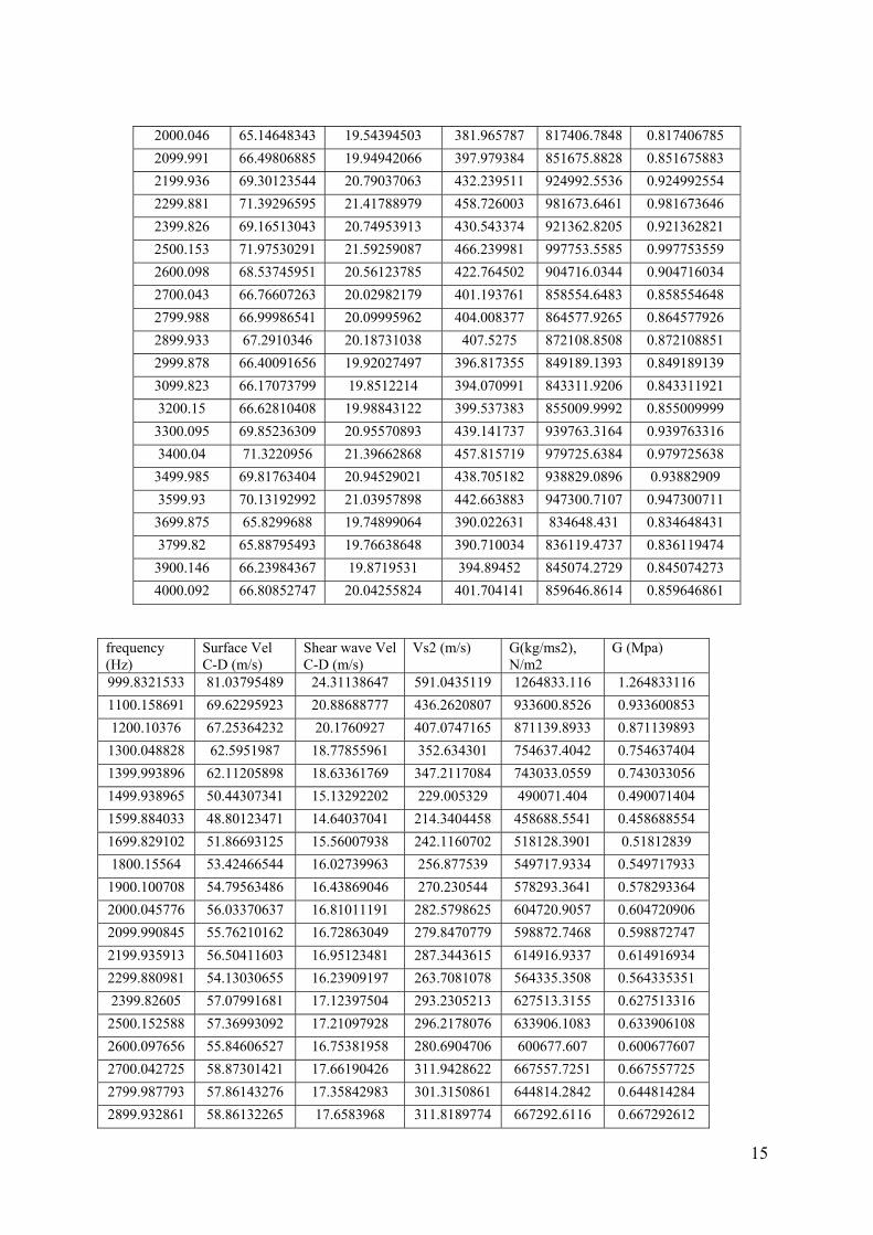
15
2000.046 65.14648343 19.54394503 381.965787 817406.7848 0.817406785
2099.991 66.49806885 19.94942066 397.979384 851675.8828 0.851675883
2199.936 69.30123544 20.79037063 432.239511 924992.5536 0.924992554
2299.881 71.39296595 21.41788979 458.726003 981673.6461 0.981673646
2399.826 69.16513043 20.74953913 430.543374 921362.8205 0.921362821
2500.153 71.97530291 21.59259087 466.239981 997753.5585 0.997753559
2600.098 68.53745951 20.56123785 422.764502 904716.0344 0.904716034
2700.043 66.76607263 20.02982179 401.193761 858554.6483 0.858554648
2799.988 66.99986541 20.09995962 404.008377 864577.9265 0.864577926
2899.933 67.2910346 20.18731038 407.5275 872108.8508 0.872108851
2999.878 66.40091656 19.92027497 396.817355 849189.1393 0.849189139
3099.823 66.17073799 19.8512214 394.070991 843311.9206 0.843311921
3200.15 66.62810408 19.98843122 399.537383 855009.9992 0.855009999
3300.095 69.85236309 20.95570893 439.141737 939763.3164 0.939763316
3400.04 71.3220956 21.39662868 457.815719 979725.6384 0.979725638
3499.985 69.81763404 20.94529021 438.705182 938829.0896 0.93882909
3599.93 70.13192992 21.03957898 442.663883 947300.7107 0.947300711
3699.875 65.8299688 19.74899064 390.022631 834648.431 0.834648431
3799.82 65.88795493 19.76638648 390.710034 836119.4737 0.836119474
3900.146 66.23984367 19.8719531 394.89452 845074.2729 0.845074273
4000.092 66.80852747 20.04255824 401.704141 859646.8614 0.859646861
frequency (Hz)
Surface Vel C-D (m/s)
Shear wave Vel C-D (m/s)
Vs2 (m/s) G(kg/ms2), N/m2
G (Mpa)
999.8321533 81.03795489 24.31138647 591.0435119 1264833.116 1.264833116
1100.158691 69.62295923 20.88688777 436.2620807 933600.8526 0.933600853
1200.10376 67.25364232 20.1760927 407.0747165 871139.8933 0.871139893
1300.048828 62.5951987 18.77855961 352.634301 754637.4042 0.754637404
1399.993896 62.11205898 18.63361769 347.2117084 743033.0559 0.743033056
1499.938965 50.44307341 15.13292202 229.005329 490071.404 0.490071404
1599.884033 48.80123471 14.64037041 214.3404458 458688.5541 0.458688554
1699.829102 51.86693125 15.56007938 242.1160702 518128.3901 0.51812839
1800.15564 53.42466544 16.02739963 256.877539 549717.9334 0.549717933
1900.100708 54.79563486 16.43869046 270.230544 578293.3641 0.578293364
2000.045776 56.03370637 16.81011191 282.5798625 604720.9057 0.604720906
2099.990845 55.76210162 16.72863049 279.8470779 598872.7468 0.598872747
2199.935913 56.50411603 16.95123481 287.3443615 614916.9337 0.614916934
2299.880981 54.13030655 16.23909197 263.7081078 564335.3508 0.564335351
2399.82605 57.07991681 17.12397504 293.2305213 627513.3155 0.627513316
2500.152588 57.36993092 17.21097928 296.2178076 633906.1083 0.633906108
2600.097656 55.84606527 16.75381958 280.6904706 600677.607 0.600677607
2700.042725 58.87301421 17.66190426 311.9428622 667557.7251 0.667557725
2799.987793 57.86143276 17.35842983 301.3150861 644814.2842 0.644814284
2899.932861 58.86132265 17.6583968 311.8189774 667292.6116 0.667292612
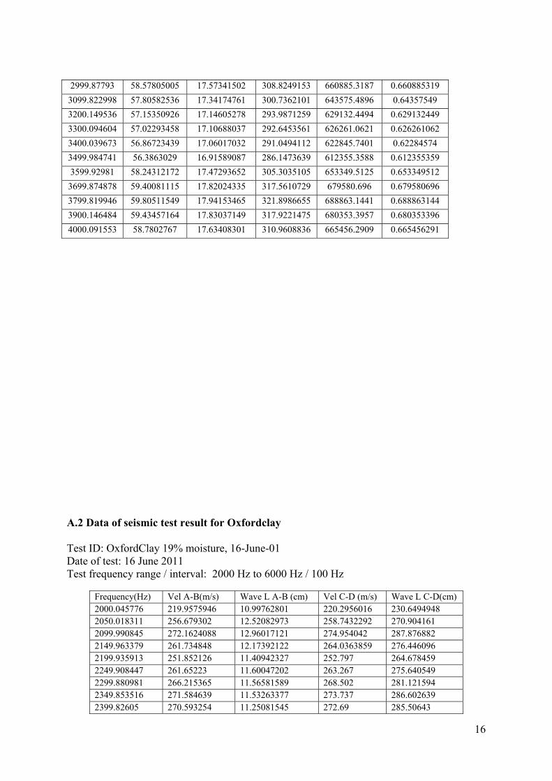
16
2999.87793 58.57805005 17.57341502 308.8249153 660885.3187 0.660885319
3099.822998 57.80582536 17.34174761 300.7362101 643575.4896 0.64357549
3200.149536 57.15350926 17.14605278 293.9871259 629132.4494 0.629132449
3300.094604 57.02293458 17.10688037 292.6453561 626261.0621 0.626261062
3400.039673 56.86723439 17.06017032 291.0494112 622845.7401 0.62284574
3499.984741 56.3863029 16.91589087 286.1473639 612355.3588 0.612355359
3599.92981 58.24312172 17.47293652 305.3035105 653349.5125 0.653349512
3699.874878 59.40081115 17.82024335 317.5610729 679580.696 0.679580696
3799.819946 59.80511549 17.94153465 321.8986655 688863.1441 0.688863144
3900.146484 59.43457164 17.83037149 317.9221475 680353.3957 0.680353396
4000.091553 58.7802767 17.63408301 310.9608836 665456.2909 0.665456291
A.2 Data of seismic test result for Oxfordclay Test ID: OxfordClay 19% moisture, 16-June-01 Date of test: 16 June 2011 Test frequency range / interval: 2000 Hz to 6000 Hz / 100 Hz
Frequency(Hz) Vel A-B(m/s) Wave L A-B (cm) Vel C-D (m/s) Wave L C-D(cm) 2000.045776 219.9575946 10.99762801 220.2956016 230.6494948 2050.018311 256.679302 12.52082973 258.7432292 270.904161 2099.990845 272.1624088 12.96017121 274.954042 287.876882 2149.963379 261.734848 12.17392122 264.0363859 276.446096 2199.935913 251.852126 11.40942327 252.797 264.678459 2249.908447 261.65223 11.60047202 263.267 275.640549 2299.880981 266.215365 11.56581589 268.502 281.121594 2349.853516 271.584639 11.53263377 273.737 286.602639 2399.82605 270.593254 11.25081545 272.69 285.50643

17
2450.180054 269.523654 10.97878499 271.643 284.410221 2500.152588 271.548563 10.83933842 273.737 286.602639 2550.125122 269.5684526 10.54850202 271.643 284.410221 2600.097656 256.548712 9.845784038 258.032 270.159504 2650.07019 259.890254 9.77332604 261.173 273.448131 2700.042725 269.521045 9.962805312 271.643 284.410221 2750.015259 268.536021 9.745400472 270.596 283.314012 2799.987793 261.008546 9.32146921 263.267 275.640549 2849.960327 265.4128027 9.29837505 267.455 280.025385 2899.932861 267.536982 9.207109708 269.549 282.217803 2949.905396 271.2536001 9.18673529 273.737 286.602639 2999.87793 267.586203 8.900362157 269.549 282.217803 3049.850464 272.101452 8.918470044 274.784 287.698848 3099.822998 274.518202 8.839214374 276.878 289.891266 3150.177002 271.0879963 8.602691209 273.737 286.602639 3200.149536 275.203698 8.593348432 277.925 290.987475 3250.12207 268.102546 8.245844131 270.596 283.314012 3300.094604 269.085479 8.15128147 271.643 284.410221 3350.067139 270.302587 8.059539968 272.69 285.50643 3400.039673 259.54893 7.617558173 261.173 273.448131 3450.012207 255.485693 7.391278195 256.985 269.063295 3499.984741 275.0719894 7.859233959 278.0003729 291.0663904 3549.957275 290.1384254 8.173011755 293.7749314 307.5823532 3599.92981 291.1145132 8.086671923 294.7968953 308.6523494 3649.902344 286.6597798 7.853902728 290.1327894 303.7690305 3699.874878 280.1200115 7.571067151 299.26359 313.053466 3749.847412 271.7956717 7.248179509 298.325471 312.006454 3799.819946 265.5276043 6.987899638 300.320145 314.124454 3850.17395 283.5519725 7.364653549 305.321475 319.3354454 3900.146484 286.4296491 7.344074133 300.201471 314.11145 3950.119019 284.26845 7.196452783 295.21493 308.865545 4000.091553 293.8042152 7.344937267 292.583 306.334401 4050.064087 297.4643534 7.344682628 288.395 301.949565 4100.036621 284.2085446 6.931853806 310.361725 324.5754 4150.009155 276.55754 6.664022407 312.980321 326.664245 4199.981689 274.0378162 6.524738355 310.0017633 324.577572 4249.954224 273.2473271 6.429418124 300.367152 314.12447 4299.926758 273.1851625 6.353251529 310.571201 324.576687 4349.899292 272.5781939 6.266310449 315.971503 329.805431 4399.871826 271.5197047 6.171082145 310.3471205 324.5775463 4449.84436 270.917851 6.088254534 273.65099 286.5125866 4499.816895 271.5768414 6.035286496 274.3409529 287.2349777 4550.170898 272.8981959 5.997537279 275.7244111 288.6834584 4600.143433 272.5261366 5.924296505 275.334865 288.2756037 4650.115967 272.6990849 5.864350197 275.5159418 288.4651911 4700.088501 275.8402863 5.868831752 278.8047798 291.9086044 4750.061035 279.8875201 5.892293131 283.0422335 296.3452185 4800.033569 283.0695939 5.897241963 290.621752 303.63463 4850.006104 283.2523021 5.840246301 280.345268 293.166456 4899.978638 280.1140002 5.716637172 280.7802549 293.16145 4949.951172 275.4860285 5.565429213 279.624105 292.113238

18
4999.923706 273.4123924 5.468331288 277.8701253 290.0196843 5049.89624 272.2456994 5.391114716 265.620514 277.4550456 5099.868774 271.5877457 5.325386941 260.32759 272.224362 5149.841309 270.7870972 5.258163911 265.378941 277.45501231 5199.813843 269.3206382 5.179428462 267.39425 279.54916401 5250.167847 266.490585 5.075848864 277.712543 290.019442 5300.140381 262.5941983 4.954476286 280.697082 293.16001 5350.112915 259.1451024 4.84373146 282.647125 295.254454 5400.085449 256.8784456 4.756932978 283.975142 296.301454 5450.057983 256.3741355 4.70406253 280.364102 293.16162 5500.030518 256.6016604 4.665458848 283.445236 296.301213 5550.003052 257.3364243 4.63668978 290.714982 303.630456 5599.975586 258.2130258 4.610966991 293.36352 306.771785 5649.94812 259.123866 4.586305228 290.02351 303.634546 5699.920654 260.5001428 4.570241564 293.201402 306.7715464 5749.893188 261.3264652 4.544892516 295.317402 308.8650134 5799.865723 261.2507241 4.504427112 285.65485 298.3951035 5849.838257 263.9378616 4.511883065 262.678219 274.3145601 5899.810791 261.7556619 4.436678924 260.634825 272.2246478 5950.164795 259.096604 4.354444169 252.541023 263.8443145 6000.137329 255.7237392 4.261964771 250.659725 261.7579301
frequency (Hz)
Surface Vel A-B (m/s)
Shear wave Vel A-B (m/s)
Vs2 (m/s) G(kg/ms2), N/m2
G (Mpa)
2000.04578 219.9575946 65.98727838 4354.320908 10102.02451 0.010102025
2050.01831 256.679302 77.0037906 5929.583767 13756.63434 0.013756634
2099.99084 272.1624088 81.64872264 6666.513909 15466.31227 0.015466312
2149.96338 261.734848 78.5204544 6165.461759 14303.87128 0.014303871
2199.93591 247.1152811 74.13458433 5495.936594 12750.5729 0.012750573
2249.90845 239.3135603 71.79406809 5154.388213 11958.18065 0.011958181
2299.88098 244.7325273 73.41975819 5390.460893 12505.86927 0.012505869
2349.85352 257.350633 77.2051899 5960.641347 13828.68793 0.013828688
2399.82605 267.9878441 80.39635323 6463.573613 14995.49078 0.014995491
2450.18005 266.5851412 79.97554236 6396.087376 14838.92271 0.014838923
2500.15259 261.6132054 78.48396162 6159.732232 14290.57878 0.014290579
2550.12512 254.596241 76.3788723 5833.732134 13534.25855 0.013534259
2600.09766 243.1379792 72.94139376 5320.446924 12343.43686 0.012343437
2650.07019 230.4873239 69.14619717 4781.196583 11092.37607 0.011092376
2700.04272 219.8703443 65.96110329 4350.867147 10094.01178 0.010094012
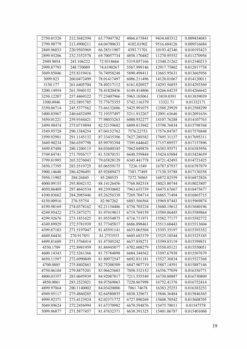
19
2750.01526 212.5682594 63.77047782 4066.673841 9434.683312 0.009434683
2799.98779 213.4900211 64.04700633 4102.01902 9516.684126 0.009516684
2849.96033 220.9503969 66.28511907 4393.71701 10193.42346 0.010193423
2899.93286 232.3352578 69.70057734 4858.170482 11270.95552 0.011270956
2949.9054 243.106222 72.9318666 5319.057166 12340.21262 0.012340213
2999.87793 248.730089 74.6190267 5567.999146 12917.75802 0.012917758
3049.85046 255.8319416 76.74958248 5890.498411 13665.95631 0.013665956
3099.823 260.0472499 78.01417497 6086.211496 14120.01067 0.014120011
3150.177 261.6405704 78.49217112 6161.020927 14293.56855 0.014293569
3200.14954 261.3940152 78.41820456 6149.414806 14266.64235 0.014266642
3250.12207 257.4469322 77.23407966 5965.103061 13839.0391 0.013839039
3300.0946 252.5891785 75.77675355 5742.116379 13321.71 0.01332171
3350.06714 245.5377562 73.66132686 5425.991075 12588.29929 0.012588299
3400.03967 240.6452499 72.19357497 5211.912267 12091.63646 0.012091636
3450.01221 259.9344421 77.98033263 6080.932277 14107.76288 0.014107763
3499.98474 275.0719894 82.52159682 6809.813942 15798.76834 0.015798768
3549.95728 290.1384254 87.04152762 7576.22753 17576.84787 0.017576848
3599.92981 291.1145132 87.33435396 7627.289382 17695.31137 0.017695311
3649.90234 286.6597798 85.99793394 7395.644642 17157.89557 0.017157896
3699.87488 280.1200115 84.03600345 7062.049876 16383.95571 0.016383956
3749.84741 271.7956717 81.53870151 6648.559844 15424.65884 0.015424659
3799.81995 265.5276043 79.65828129 6345.441778 14721.42493 0.014721425
3850.17395 283.5519725 85.06559175 7236.1549 16787.87937 0.016787879
3900.14648 286.4296491 85.92889473 7383.77495 17130.35788 0.017130358
3950.11902 284.26845 85.280535 7272.76965 16872.82559 0.016872826
4000.09155 293.8042152 88.14126456 7768.882518 18023.80744 0.018023807
4050.06409 297.4643534 89.23930602 7963.653739 18475.67667 0.018475677
4100.03662 284.2085446 85.26256338 7269.704714 16865.71494 0.016865715
4150.00916 276.55754 82.967262 6883.566564 15969.87443 0.015969874
4199.98169 274.0378162 82.21134486 6758.705224 15680.19612 0.015680196
4249.95422 273.2473271 81.97419813 6719.769159 15589.86445 0.015589864
4299.92676 273.1851625 81.95554875 6716.711971 15582.77177 0.015582772
4349.89929 272.5781939 81.77345817 6686.898461 15513.60443 0.015513604
4399.87183 271.5197047 81.45591141 6635.065504 15393.35197 0.015393352
4449.84436 270.917851 81.2753553 6605.683379 15325.18544 0.015325185
4499.81689 271.5768414 81.47305242 6637.858271 15399.83119 0.015399831
4550.1709 272.8981959 81.86945877 6702.608279 15550.05121 0.015550051
4600.14343 272.5261366 81.75784098 6684.344562 15507.67938 0.015507679
4650.11597 272.6990849 81.80972547 6692.831181 15527.36834 0.015527368
4700.0885 275.8402863 82.75208589 6847.907719 15887.14591 0.015887146
4750.06104 279.8875201 83.96625603 7050.332152 16356.77059 0.016356771
4800.03357 283.0695939 84.92087817 7211.555549 16730.80887 0.016730809
4850.0061 283.2523021 84.97569063 7220.867998 16752.41376 0.016752414
4899.97864 280.1140002 84.03420006 7061.74678 16383.25253 0.016383253
4949.95117 275.4860285 82.64580855 6830.329671 15846.36484 0.015846365
4999.92371 273.4123924 82.02371772 6727.890269 15608.70542 0.015608705
5049.89624 272.2456994 81.67370982 6670.594876 15475.78011 0.01547578
5099.86877 271.5877457 81.47632371 6638.391325 15401.06787 0.015401068
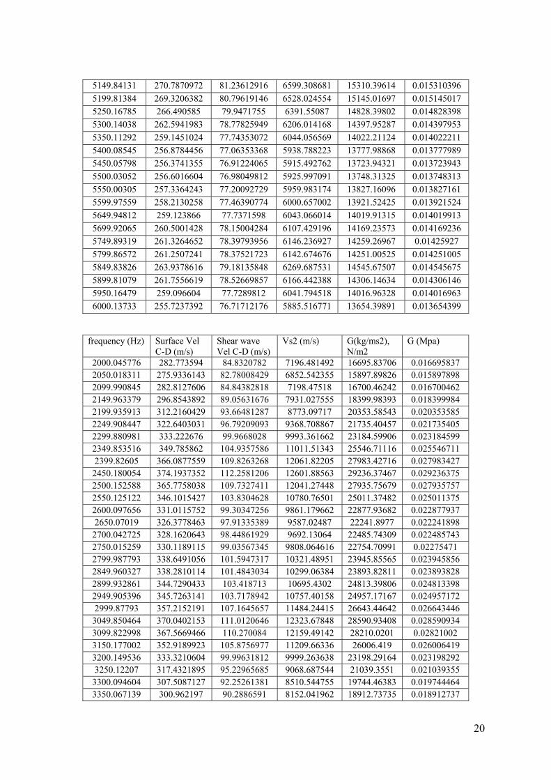
20
5149.84131 270.7870972 81.23612916 6599.308681 15310.39614 0.015310396
5199.81384 269.3206382 80.79619146 6528.024554 15145.01697 0.015145017
5250.16785 266.490585 79.9471755 6391.55087 14828.39802 0.014828398
5300.14038 262.5941983 78.77825949 6206.014168 14397.95287 0.014397953
5350.11292 259.1451024 77.74353072 6044.056569 14022.21124 0.014022211
5400.08545 256.8784456 77.06353368 5938.788223 13777.98868 0.013777989
5450.05798 256.3741355 76.91224065 5915.492762 13723.94321 0.013723943
5500.03052 256.6016604 76.98049812 5925.997091 13748.31325 0.013748313
5550.00305 257.3364243 77.20092729 5959.983174 13827.16096 0.013827161
5599.97559 258.2130258 77.46390774 6000.657002 13921.52425 0.013921524
5649.94812 259.123866 77.7371598 6043.066014 14019.91315 0.014019913
5699.92065 260.5001428 78.15004284 6107.429196 14169.23573 0.014169236
5749.89319 261.3264652 78.39793956 6146.236927 14259.26967 0.01425927
5799.86572 261.2507241 78.37521723 6142.674676 14251.00525 0.014251005
5849.83826 263.9378616 79.18135848 6269.687531 14545.67507 0.014545675
5899.81079 261.7556619 78.52669857 6166.442388 14306.14634 0.014306146
5950.16479 259.096604 77.7289812 6041.794518 14016.96328 0.014016963
6000.13733 255.7237392 76.71712176 5885.516771 13654.39891 0.013654399
frequency (Hz) Surface Vel C-D (m/s)
Shear wave Vel C-D (m/s)
Vs2 (m/s) G(kg/ms2), N/m2
G (Mpa)
2000.045776 282.773594 84.8320782 7196.481492 16695.83706 0.016695837 2050.018311 275.9336143 82.78008429 6852.542355 15897.89826 0.015897898 2099.990845 282.8127606 84.84382818 7198.47518 16700.46242 0.016700462 2149.963379 296.8543892 89.05631676 7931.027555 18399.98393 0.018399984 2199.935913 312.2160429 93.66481287 8773.09717 20353.58543 0.020353585 2249.908447 322.6403031 96.79209093 9368.708867 21735.40457 0.021735405 2299.880981 333.222676 99.9668028 9993.361662 23184.59906 0.023184599 2349.853516 349.785862 104.9357586 11011.51343 25546.71116 0.025546711 2399.82605 366.0877559 109.8263268 12061.82205 27983.42716 0.027983427
2450.180054 374.1937352 112.2581206 12601.88563 29236.37467 0.029236375 2500.152588 365.7758038 109.7327411 12041.27448 27935.75679 0.027935757 2550.125122 346.1015427 103.8304628 10780.76501 25011.37482 0.025011375 2600.097656 331.0115752 99.30347256 9861.179662 22877.93682 0.022877937 2650.07019 326.3778463 97.91335389 9587.02487 22241.8977 0.022241898
2700.042725 328.1620643 98.44861929 9692.13064 22485.74309 0.022485743 2750.015259 330.1189115 99.03567345 9808.064616 22754.70991 0.02275471 2799.987793 338.6491056 101.5947317 10321.48951 23945.85565 0.023945856 2849.960327 338.2810114 101.4843034 10299.06384 23893.82811 0.023893828 2899.932861 344.7290433 103.418713 10695.4302 24813.39806 0.024813398 2949.905396 345.7263141 103.7178942 10757.40158 24957.17167 0.024957172 2999.87793 357.2152191 107.1645657 11484.24415 26643.44642 0.026643446
3049.850464 370.0402153 111.0120646 12323.67848 28590.93408 0.028590934 3099.822998 367.5669466 110.270084 12159.49142 28210.0201 0.02821002 3150.177002 352.9189923 105.8756977 11209.66336 26006.419 0.026006419 3200.149536 333.3210604 99.99631812 9999.263638 23198.29164 0.023198292 3250.12207 317.4321895 95.22965685 9068.687544 21039.3551 0.021039355
3300.094604 307.5087127 92.25261381 8510.544755 19744.46383 0.019744464 3350.067139 300.962197 90.2886591 8152.041962 18912.73735 0.018912737
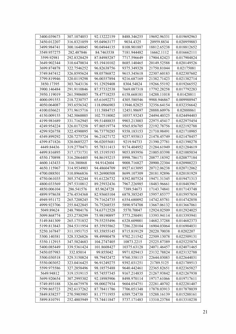
21
3400.039673 307.1074053 92.13222159 8488.346255 19692.96331 0.019692963 3450.012207 316.8321059 95.04963177 9034.4325 20959.8834 0.020959883 3499.984741 300.1648045 90.04944135 8108.901887 18812.65238 0.018812652 3549.957275 282.487846 84.7463538 7181.944482 16662.1112 0.016662111 3599.92981 292.8328429 87.84985287 7717.596649 17904.82423 0.017904824
3649.902344 310.6470034 93.19410102 8685.140465 20149.52588 0.020149526 3699.874878 322.7546252 96.82638756 9375.349328 21750.81044 0.02175081 3749.847412 326.8595624 98.05786872 9615.345618 22307.60183 0.022307602 3799.819946 320.0119298 96.00357894 9216.687169 21382.71423 0.021382714 3850.17395 303.7643136 91.12929408 8304.54824 19266.55192 0.019266552
3900.146484 291.9110846 87.57332538 7669.087318 17792.28258 0.017792283 3950.119019 261.5906085 78.47718255 6158.668181 14288.11018 0.01428811 4000.091553 218.7230757 65.61692271 4305.580546 9988.946867 0.009988947 4050.064087 393.6556342 118.0966903 13946.82825 32356.64154 0.032356642 4100.036621 371.9615716 111.5884715 12451.98697 28888.60976 0.02888861 4150.009155 342.5060005 102.7518002 10557.93243 24494.40325 0.024494403 4199.981689 331.7162945 99.51488835 9903.213003 22975.45417 0.022975454 4249.954224 326.0173258 97.80519774 9565.856705 22192.78756 0.022192788 4299.926758 322.4590095 96.73770285 9358.183153 21710.98491 0.021710985 4349.899292 320.7275724 96.21827172 9257.955813 21478.45749 0.021478457 4399.871826 320.0685227 96.02055681 9219.94733 21390.27781 0.021390278 4449.84436 319.2770471 95.78311413 9174.404952 21284.61949 0.021284619
4499.816895 317.1731731 95.15195193 9053.893956 21005.03398 0.021005034 4550.170898 316.2064405 94.86193215 8998.786171 20877.18392 0.020877184 4600.143433 316.380868 94.9142604 9008.716827 20900.22304 0.020900223 4650.115967 314.9534903 94.48604709 8927.613095 20712.06238 0.020712062 4700.088501 310.8966836 93.26900508 8699.107309 20181.92896 0.020181929 4750.061035 305.3742244 91.61226732 8392.807524 19471.31345 0.019471313 4800.033569 297.5310812 89.25932436 7967.226985 18483.96661 0.018483967 4850.006104 286.541576 85.9624728 7389.54673 17143.74841 0.017143748 4899.978638 276.4534368 82.93603104 6878.385245 15957.85377 0.015957854 4949.951172 265.7208245 79.71624735 6354.680092 14742.85781 0.014742858 4999.923706 255.8422845 76.75268535 5890.974708 13667.06132 0.013667061 5049.89624 248.7904176 74.63712528 5570.70047 12924.02509 0.012924025
5099.868774 253.2730299 75.98190897 5773.250491 13393.94114 0.013393941 5149.841309 265.1751832 79.55255496 6328.609001 14682.37288 0.014682373 5199.813843 284.5311954 85.35935862 7286.220104 16904.03064 0.016904031 5250.167847 311.1951715 93.35855145 8715.819129 20220.70038 0.0202207 5300.140381 328.3326826 98.49980478 9702.211542 22509.13078 0.022509131 5350.112915 347.5824683 104.2747405 10873.2215 25225.87389 0.025225874 5400.085449 339.5361424 101.8608427 10375.63128 24071.46457 0.024071465 5450.057983 332.85014 99.855042 9971.029413 23132.78824 0.023132788 5500.030518 329.3150824 98.79452472 9760.358115 22644.03083 0.022644031 5550.003052 323.0416425 96.91249275 9392.031251 21789.5125 0.021789513 5599.975586 327.2858496 98.18575488 9640.442461 22365.82651 0.022365827 5649.94812 319.1519115 95.74557345 9167.214835 21267.93842 0.021267938
5699.920654 307.2995302 92.18985906 8498.970114 19717.61066 0.019717611 5749.893188 326.6675978 98.00027934 9604.054751 22281.40702 0.022281407 5799.865723 292.6137262 87.78411786 7706.051348 17878.03913 0.017878039 5849.838257 270.5903985 81.17711955 6589.724738 15288.16139 0.015288161 5899.810791 252.4803949 75.74411847 5737.171483 13310.23784 0.013310238
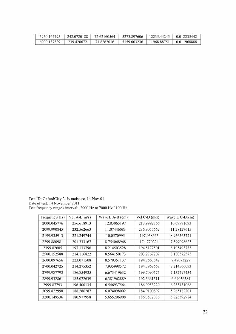
22
5950.164795 242.0720188 72.62160564 5273.897606 12235.44245 0.012235442 6000.137329 239.420672 71.8262016 5159.003236 11968.88751 0.011968888
Test ID: OxfordClay 24% moisture, 14-Nov-01 Date of test: 14 November 2011 Test frequency range / interval: 2000 Hz to 7000 Hz / 100 Hz
Frequency(Hz) Vel A-B(m/s) Wave L A-B (cm) Vel C-D (m/s) Wave L C-D(cm)
2000.045776 256.618913 12.83065197 213.9992366 10.69971693
2099.990845 232.562663 11.07446083 236.9057662 11.28127615
2199.935913 221.249744 10.0570995 197.038663 8.956563771
2299.880981 201.333167 8.754068968 174.770224 7.599098623
2399.82605 197.133796 8.214503528 194.5177501 8.105493733
2500.152588 214.116822 8.564150173 203.2767207 8.130572575
2600.097656 223.071508 8.579351137 194.7663542 7.49073227
2700.042725 214.275352 7.935998572 194.7963669 7.214566093
2799.987793 186.854935 6.673419632 199.7090575 7.132497434
2899.932861 185.072639 6.381962889 192.5661511 6.64036584
2999.87793 196.400135 6.546937564 186.9953229 6.233431068
3099.822998 188.286287 6.074098002 184.9100897 5.965182201
3200.149536 180.977958 5.655296908 186.3572836 5.823392984
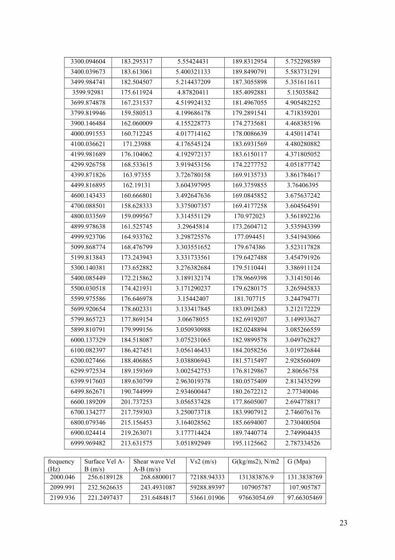
23
3300.094604 183.295317 5.55424431 189.8312954 5.752298589
3400.039673 183.613061 5.400321133 189.8490791 5.583731291
3499.984741 182.504507 5.214437209 187.3055898 5.351611611
3599.92981 175.611924 4.87820411 185.4092881 5.15035842
3699.874878 167.231537 4.519924132 181.4967055 4.905482252
3799.819946 159.580513 4.199686178 179.2891541 4.718359201
3900.146484 162.060009 4.155228773 174.2735681 4.468385196
4000.091553 160.712245 4.017714162 178.0086639 4.450114741
4100.036621 171.23988 4.176545124 183.6931569 4.480280882
4199.981689 176.104062 4.192972137 183.6150117 4.371805052
4299.926758 168.533615 3.919453156 174.2277752 4.051877742
4399.871826 163.97355 3.726780158 169.9135733 3.861784617
4499.816895 162.19131 3.604397995 169.3759855 3.76406395
4600.143433 160.666801 3.492647636 169.0845852 3.675637242
4700.088501 158.628333 3.375007357 169.4177258 3.604564591
4800.033569 159.099567 3.314551129 170.972023 3.561892236
4899.978638 161.525745 3.29645814 173.2604712 3.535943399
4999.923706 164.933762 3.298725576 177.094451 3.541943066
5099.868774 168.476799 3.303551652 179.674386 3.523117828
5199.813843 173.243943 3.331733561 179.6427488 3.454791926
5300.140381 173.652882 3.276382684 179.5110441 3.386911124
5400.085449 172.215862 3.189132174 178.9669398 3.314150146
5500.030518 174.421931 3.171290237 179.6280175 3.265945833
5599.975586 176.646978 3.15442407 181.707715 3.244794771
5699.920654 178.602331 3.133417845 183.0912683 3.212172229
5799.865723 177.869154 3.06678055 182.6919207 3.149933627
5899.810791 179.999156 3.050930988 182.0248894 3.085266559
6000.137329 184.518087 3.075231065 182.9899578 3.049762827
6100.082397 186.427451 3.056146433 184.2058256 3.019726844
6200.027466 188.406865 3.038806943 181.5715497 2.928560409
6299.972534 189.159369 3.002542753 176.8129867 2.80656758
6399.917603 189.630799 2.963019378 180.0575409 2.813435299
6499.862671 190.744999 2.934600447 180.2672212 2.77340046
6600.189209 201.737253 3.056537428 177.8605007 2.694778817
6700.134277 217.759303 3.250073718 183.9907912 2.746076176
6800.079346 215.156453 3.164028562 185.6694007 2.730400504
6900.024414 219.263071 3.177714424 189.7440774 2.749904435
6999.969482 213.631575 3.051892949 195.1125662 2.787334526
frequency (Hz)
Surface Vel A-B (m/s)
Shear wave Vel A-B (m/s)
Vs2 (m/s) G(kg/ms2), N/m2 G (Mpa)
2000.046 256.6189128 268.6800017 72188.94333 131383876.9 131.3838769
2099.991 232.5626635 243.4931087 59288.89397 107905787 107.905787
2199.936 221.2497437 231.6484817 53661.01906 97663054.69 97.66305469
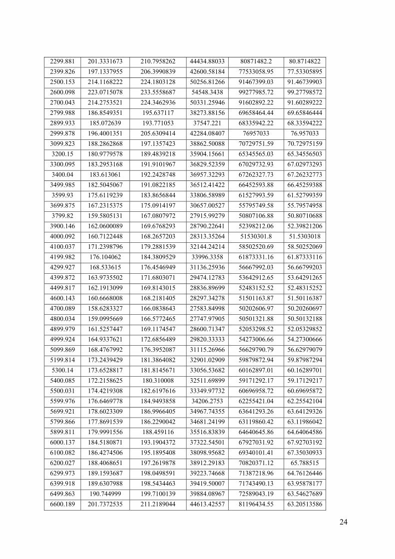
24
2299.881 201.3331673 210.7958262 44434.88033 80871482.2 80.8714822
2399.826 197.1337955 206.3990839 42600.58184 77533058.95 77.53305895
2500.153 214.1168222 224.1803128 50256.81266 91467399.03 91.46739903
2600.098 223.0715078 233.5558687 54548.3438 99277985.72 99.27798572
2700.043 214.2753521 224.3462936 50331.25946 91602892.22 91.60289222
2799.988 186.8549351 195.637117 38273.88156 69658464.44 69.65846444
2899.933 185.072639 193.771053 37547.221 68335942.22 68.33594222
2999.878 196.4001351 205.6309414 42284.08407 76957033 76.957033
3099.823 188.2862868 197.1357423 38862.50088 70729751.59 70.72975159
3200.15 180.9779578 189.4839218 35904.15661 65345565.03 65.34556503
3300.095 183.2953168 191.9101967 36829.52359 67029732.93 67.02973293
3400.04 183.613061 192.2428748 36957.32293 67262327.73 67.26232773
3499.985 182.5045067 191.0822185 36512.41422 66452593.88 66.45259388
3599.93 175.6119239 183.8656844 33806.58989 61527993.59 61.52799359
3699.875 167.2315375 175.0914197 30657.00527 55795749.58 55.79574958
3799.82 159.5805131 167.0807972 27915.99279 50807106.88 50.80710688
3900.146 162.0600089 169.6768293 28790.22641 52398212.06 52.39821206
4000.092 160.7122448 168.2657203 28313.35264 51530301.8 51.5303018
4100.037 171.2398796 179.2881539 32144.24214 58502520.69 58.50252069
4199.982 176.104062 184.3809529 33996.3358 61873331.16 61.87333116
4299.927 168.533615 176.4546949 31136.25936 56667992.03 56.66799203
4399.872 163.9735502 171.6803071 29474.12783 53642912.65 53.64291265
4499.817 162.1913099 169.8143015 28836.89699 52483152.52 52.48315252
4600.143 160.6668008 168.2181405 28297.34278 51501163.87 51.50116387
4700.089 158.6283327 166.0838643 27583.84998 50202606.97 50.20260697
4800.034 159.0995669 166.5772465 27747.97905 50501321.88 50.50132188
4899.979 161.5257447 169.1174547 28600.71347 52053298.52 52.05329852
4999.924 164.9337621 172.6856489 29820.33333 54273006.66 54.27300666
5099.869 168.4767992 176.3952087 31115.26966 56629790.79 56.62979079
5199.814 173.2439429 181.3864082 32901.02909 59879872.94 59.87987294
5300.14 173.6528817 181.8145671 33056.53682 60162897.01 60.16289701
5400.085 172.2158625 180.310008 32511.69899 59171292.17 59.17129217
5500.031 174.4219308 182.6197616 33349.97732 60696958.72 60.69695872
5599.976 176.6469778 184.9493858 34206.2753 62255421.04 62.25542104
5699.921 178.6023309 186.9966405 34967.74355 63641293.26 63.64129326
5799.866 177.8691539 186.2290042 34681.24199 63119860.42 63.11986042
5899.811 179.9991556 188.459116 35516.83839 64640645.86 64.64064586
6000.137 184.5180871 193.1904372 37322.54501 67927031.92 67.92703192
6100.082 186.4274506 195.1895408 38098.95682 69340101.41 67.35030933
6200.027 188.4068651 197.2619878 38912.29183 70820371.12 65.788515
6299.973 189.1593687 198.0498591 39223.74668 71387218.96 64.76126446
6399.918 189.6307988 198.5434463 39419.50007 71743490.13 63.95878177
6499.863 190.744999 199.7100139 39884.08967 72589043.19 63.54627689
6600.189 201.7372535 211.2189044 44613.42557 81196434.55 63.20513586

25
6700.134 217.7593032 227.9939905 51981.2597 94605892.65 62.51581237
6800.079 215.1564527 225.268806 50746.03496 92357783.62 61.61917399
6900.024 219.2630711 229.5684354 52701.66654 95917033.1 60.88786379
6999.969 213.6315751 223.6722591 50029.2795 91053288.7 60.6739467
frequency (Hz)
Surface Vel C-D (m/s)
Shear wave Vel C-D (m/s)
Vs2 (m/s) G(kg/ms2), N/m2
G (Mpa)
2000.04578 213.9992366 224.0572007 50201.6292 91366965.13 91.36696513
2099.99084 236.9057662 248.0403373 61524.0089 111973696.2 111.9736962
2199.93591 197.038663 206.2994801 42559.4755 77458245.42 77.45824542
2299.88098 174.770224 182.9844245 33483.2996 60939605.3 60.9396053
2399.82605 194.5177501 203.6600843 41477.4299 75488922.5 75.4889225
2500.15259 203.2767207 212.8307265 45296.9182 82440391.04 82.44039104
2600.09766 194.7663542 203.9203728 41583.5185 75682003.59 75.68200359
2700.04272 194.7963669 203.9517962 41596.3352 75705329.99 75.70532999
2799.98779 199.7090575 209.0953832 43720.8793 79572000.27 79.57200027
2899.93286 192.5661511 201.6167602 40649.318 73981758.75 73.98175875
2999.87793 186.9953229 195.7841031 38331.415 69763175.31 69.76317531
3099.823 184.9100897 193.600864 37481.2945 68215956.04 68.21595604
3200.14954 186.3572836 195.1160759 38070.2831 69287915.19 69.28791519
3300.0946 189.8312954 198.7533663 39502.9006 71895279.09 71.89527909
3400.03967 189.8490791 198.7719858 39510.3024 71908750.28 71.90875028
3499.98474 187.3055898 196.1089525 38458.7213 69994872.68 69.99487268
3599.92981 185.4092881 194.1235246 37683.9428 68584775.91 68.58477591
3699.87488 181.4967055 190.0270506 36110.28 65720709.56 65.72070956
3799.81995 179.2891541 187.7157443 35237.2007 64131705.2 64.1317052
3900.14648 174.2735681 182.4644258 33293.2667 60593745.39 60.59374539
4000.09155 178.0086639 186.3750711 34735.6671 63218914.14 63.21891414
4100.03662 183.6931569 192.3267353 36989.5731 67321023.03 67.32102303
4199.98169 183.6150117 192.2449172 36958.1082 67263756.91 67.26375691
4299.92676 174.2277752 182.4164807 33275.7724 60561905.8 60.5619058
4399.87183 169.9135733 177.8995113 31648.2361 57599789.73 57.59978973
4499.81689 169.3759855 177.3366569 31448.2899 57235887.55 57.23588755
4600.14343 169.0845852 177.0315607 31340.1735 57039115.74 57.03911574
4700.0885 169.4177258 177.380359 31463.7917 57264100.97 57.26410097
4800.03357 170.972023 179.0077081 32043.7596 58319642.41 58.31964241
4899.97864 173.2604712 181.4037133 32907.3072 59891299.12 59.89129912
4999.92371 177.094451 185.4178902 34379.794 62571225.1 62.5712251
5099.86877 179.674386 188.1190822 35388.7891 64407596.11 64.40759611
5199.81384 179.6427488 188.085958 35376.3276 64384916.21 64.38491621
5300.14038 179.5110441 187.9480632 35324.4745 64290543.53 64.29054353
5400.08545 178.9669398 187.378386 35110.6595 63901400.36 63.90140036
5500.03052 179.6280175 188.0705343 35370.5259 64374357.12 64.37435712
5599.97559 181.707715 190.2479776 36194.293 65873613.24 65.87361324

26
5699.92065 183.0912683 191.696558 36747.5703 66880578.01 66.88057801
5799.86572 182.6919207 191.278441 36587.442 66589144.43 66.58914443
5899.81079 182.0248894 190.5800592 36320.759 66103781.32 66.10378132
6000.13733 182.9899578 191.5904858 36706.9143 66806583.95 66.80658395
6100.0824 184.2058256 192.8634995 37196.3294 67697319.55 67.69731955
6200.02747 181.5715497 190.1054125 36140.0679 65774923.52 65.77492352
6299.97253 176.8129867 185.123197 34270.5981 62372488.52 62.37248852
6399.9176 180.0575409 188.5202454 35539.8829 64682586.9 64.6825869
6499.86267 180.2672212 188.7397806 35622.7048 64833322.69 64.83332269
6600.18921 177.8605007 186.2199442 34677.8676 63113719.1 63.1137191
6700.13428 183.9907912 192.6383584 37109.5371 67539357.54 67.53935754
6800.07935 185.6694007 194.3958626 37789.7514 68777347.52 68.77734752
6900.02441 189.7440774 198.662049 39466.6097 71829229.7 71.8292297
6999.96948 195.1125662 204.2828568 41731.4856 75951303.76 75.95130376
Test ID: OxfordClay 30% moisture, 25-July-01 Date of test: 25 July 2011 Test frequency range / interval: 1000 Hz to 5000 Hz / 100 Hz Frequency(Hz) Vel A-B(m/s) Wave L A-B (cm) Vel C-D (m/s) Wave L C-D(cm)
999.8321533 101.1292882 10.11462653 122.863074 12.28836995
1100.158691 128.2139408 11.65413152 96.0938103 8.73454085
1200.10376 146.9821178 12.24745083 125.258279 10.43728743
1300.048828 171.2272322 13.17083086 123.969344 9.535745248
1399.993896 139.0189473 9.929968102 110.860373 7.918632617
1499.938965 116.0607814 7.737700273 96.7084521 6.447492487
1599.884033 114.3019231 7.144388015 96.0449007 6.003241402
1699.829102 126.153479 7.421538958 108.505855 6.38333906
1800.15564 132.0454446 7.33522378 105.88321 5.881891962
1900.100708 130.7638093 6.881940979 97.6697643 5.140241456
2000.045776 127.4345209 6.37158021 97.5383705 4.876806904
2099.990845 133.2560669 6.345554659 100.357018 4.778926454
2199.935913 135.8262225 6.17409906 103.481563 4.703844433
2299.880981 131.8694597 5.733751474 101.845339 4.428287374
2399.82605 132.0481709 5.502405933 100.532296 4.189149289

27
2500.152588 138.2984756 5.531601404 103.480206 4.138955629
2600.097656 137.8886209 5.303209306 109.087496 4.195515352
2700.042725 129.4761766 4.795338068 110.093088 4.077457241
2799.987793 122.608828 4.378905804 108.795041 3.885554102
2899.932861 120.4895906 4.15490966 106.530306 3.673543859
2999.87793 123.128992 4.104466746 105.807936 3.52707471
3099.822998 125.8247161 4.059093573 106.136794 3.423963051
3200.149536 125.1086751 3.909463406 105.733572 3.304019738
3300.094604 123.1329975 3.73119599 105.6035 3.200014321
3400.039673 122.0737319 3.590361985 108.634537 3.195096151
3499.984741 120.7573289 3.450224439 113.543408 3.244111522
3599.92981 120.2349532 3.33992493 120.869747 3.357558444
3699.874878 121.2837171 3.278049153 121.707387 3.289500073
3799.819946 122.1982778 3.215896531 121.261302 3.1912381
3900.146484 122.4799187 3.140392782 121.79363 3.122796299
4000.091553 123.0358067 3.075824769 123.810359 3.09518814
4100.036621 123.3032152 3.007368631 130.771026 3.189508736
4199.981689 125.0934756 2.978429072 130.658745 3.110936069
4299.926758 126.0563717 2.931593463 130.009938 3.023538437
4399.871826 126.0059791 2.863855677 131.728643 2.99392001
4499.816895 124.1891808 2.759871873 134.550884 2.990141312
4600.143433 122.497712 2.662910706 136.01688 2.95679651
4700.088501 121.5443642 2.586001608 138.092142 2.938075361
4800.033569 118.1210386 2.46083776 142.316819 2.964912991
4899.978638 118.8783942 2.426100254 142.738819 2.913049828
4999.923706 117.725491 2.354545748 142.481371 2.849670909
frequency (Hz)
Surface Vel A-B (m/s)
Shear wave Vel A-B (m/s)
Vs2 (m/s) G(kg/ms2), N/m2
G (Mpa)
999.8322 101.1292882 105.8823648 11211.0752 20964710.56 20.96471056
1100.159 128.2139408 134.239996 18020.3765 33698104.1 33.6981041
1200.104 146.9821178 153.8902774 23682.2175 44285746.66 44.28574666
1300.049 130 136.11 18525.9321 34643493.03 34.64349303
1399.994 139.0189473 145.5528379 21185.6286 39617125.51 39.61712551
1499.939 116.0607814 121.5156381 14766.0503 27612514.07 27.61251407
1599.884 114.3019231 119.6741135 14321.8934 26781940.74 26.78194074
1699.829 126.153479 132.0826925 17445.8377 32623716.42 32.62371642
1800.156 132.0454446 138.2515805 19113.4995 35742244.06 35.74224406
1900.101 130.7638093 136.9097083 18744.2682 35051781.59 35.05178159
2000.046 127.4345209 133.4239434 17801.9487 33289643.99 33.28964399
2099.991 133.2560669 139.519102 19465.5798 36400634.28 36.40063428
2199.936 135.8262225 142.210055 20223.6997 37818318.51 37.81831851
2299.881 131.8694597 138.0673243 19062.586 35647035.89 35.64703589
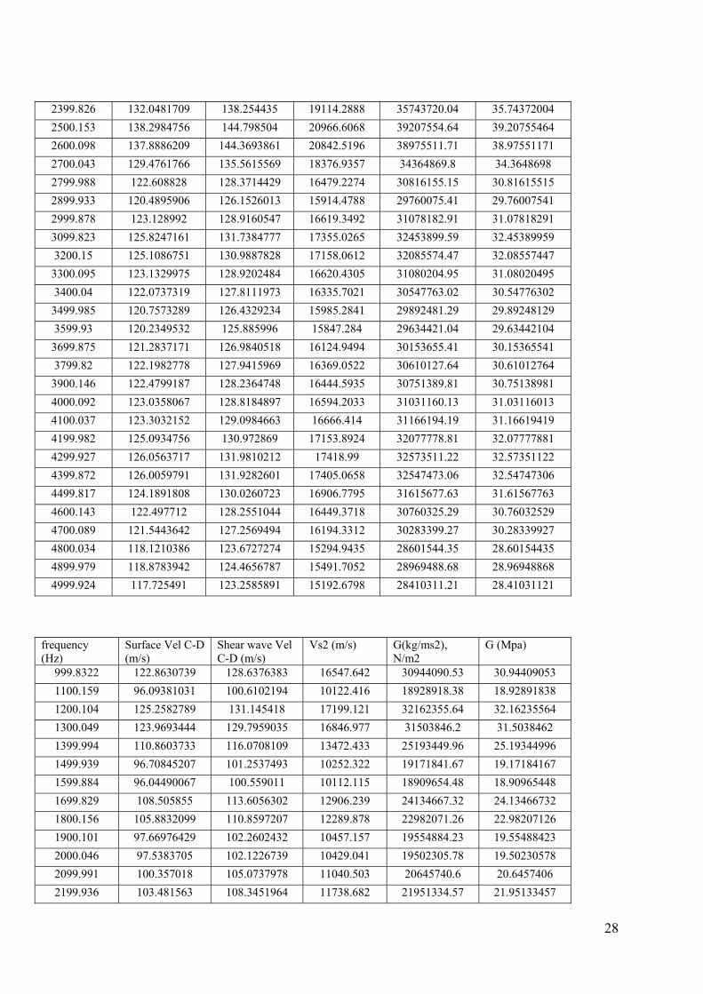
28
2399.826 132.0481709 138.254435 19114.2888 35743720.04 35.74372004
2500.153 138.2984756 144.798504 20966.6068 39207554.64 39.20755464
2600.098 137.8886209 144.3693861 20842.5196 38975511.71 38.97551171
2700.043 129.4761766 135.5615569 18376.9357 34364869.8 34.3648698
2799.988 122.608828 128.3714429 16479.2274 30816155.15 30.81615515
2899.933 120.4895906 126.1526013 15914.4788 29760075.41 29.76007541
2999.878 123.128992 128.9160547 16619.3492 31078182.91 31.07818291
3099.823 125.8247161 131.7384777 17355.0265 32453899.59 32.45389959
3200.15 125.1086751 130.9887828 17158.0612 32085574.47 32.08557447
3300.095 123.1329975 128.9202484 16620.4305 31080204.95 31.08020495
3400.04 122.0737319 127.8111973 16335.7021 30547763.02 30.54776302
3499.985 120.7573289 126.4329234 15985.2841 29892481.29 29.89248129
3599.93 120.2349532 125.885996 15847.284 29634421.04 29.63442104
3699.875 121.2837171 126.9840518 16124.9494 30153655.41 30.15365541
3799.82 122.1982778 127.9415969 16369.0522 30610127.64 30.61012764
3900.146 122.4799187 128.2364748 16444.5935 30751389.81 30.75138981
4000.092 123.0358067 128.8184897 16594.2033 31031160.13 31.03116013
4100.037 123.3032152 129.0984663 16666.414 31166194.19 31.16619419
4199.982 125.0934756 130.972869 17153.8924 32077778.81 32.07777881
4299.927 126.0563717 131.9810212 17418.99 32573511.22 32.57351122
4399.872 126.0059791 131.9282601 17405.0658 32547473.06 32.54747306
4499.817 124.1891808 130.0260723 16906.7795 31615677.63 31.61567763
4600.143 122.497712 128.2551044 16449.3718 30760325.29 30.76032529
4700.089 121.5443642 127.2569494 16194.3312 30283399.27 30.28339927
4800.034 118.1210386 123.6727274 15294.9435 28601544.35 28.60154435
4899.979 118.8783942 124.4656787 15491.7052 28969488.68 28.96948868
4999.924 117.725491 123.2585891 15192.6798 28410311.21 28.41031121
frequency (Hz)
Surface Vel C-D (m/s)
Shear wave Vel C-D (m/s)
Vs2 (m/s) G(kg/ms2), N/m2
G (Mpa)
999.8322 122.8630739 128.6376383 16547.642 30944090.53 30.94409053
1100.159 96.09381031 100.6102194 10122.416 18928918.38 18.92891838
1200.104 125.2582789 131.145418 17199.121 32162355.64 32.16235564
1300.049 123.9693444 129.7959035 16846.977 31503846.2 31.5038462
1399.994 110.8603733 116.0708109 13472.433 25193449.96 25.19344996
1499.939 96.70845207 101.2537493 10252.322 19171841.67 19.17184167
1599.884 96.04490067 100.559011 10112.115 18909654.48 18.90965448
1699.829 108.505855 113.6056302 12906.239 24134667.32 24.13466732
1800.156 105.8832099 110.8597207 12289.878 22982071.26 22.98207126
1900.101 97.66976429 102.2602432 10457.157 19554884.23 19.55488423
2000.046 97.5383705 102.1226739 10429.041 19502305.78 19.50230578
2099.991 100.357018 105.0737978 11040.503 20645740.6 20.6457406
2199.936 103.481563 108.3451964 11738.682 21951334.57 21.95133457
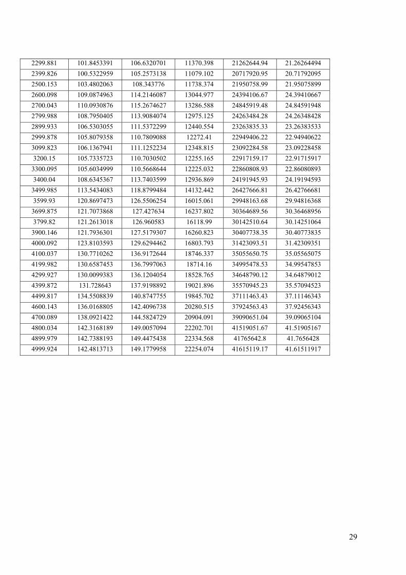
29
2299.881 101.8453391 106.6320701 11370.398 21262644.94 21.26264494
2399.826 100.5322959 105.2573138 11079.102 20717920.95 20.71792095
2500.153 103.4802063 108.343776 11738.374 21950758.99 21.95075899
2600.098 109.0874963 114.2146087 13044.977 24394106.67 24.39410667
2700.043 110.0930876 115.2674627 13286.588 24845919.48 24.84591948
2799.988 108.7950405 113.9084074 12975.125 24263484.28 24.26348428
2899.933 106.5303055 111.5372299 12440.554 23263835.33 23.26383533
2999.878 105.8079358 110.7809088 12272.41 22949406.22 22.94940622
3099.823 106.1367941 111.1252234 12348.815 23092284.58 23.09228458
3200.15 105.7335723 110.7030502 12255.165 22917159.17 22.91715917
3300.095 105.6034999 110.5668644 12225.032 22860808.93 22.86080893
3400.04 108.6345367 113.7403599 12936.869 24191945.93 24.19194593
3499.985 113.5434083 118.8799484 14132.442 26427666.81 26.42766681
3599.93 120.8697473 126.5506254 16015.061 29948163.68 29.94816368
3699.875 121.7073868 127.427634 16237.802 30364689.56 30.36468956
3799.82 121.2613018 126.960583 16118.99 30142510.64 30.14251064
3900.146 121.7936301 127.5179307 16260.823 30407738.35 30.40773835
4000.092 123.8103593 129.6294462 16803.793 31423093.51 31.42309351
4100.037 130.7710262 136.9172644 18746.337 35055650.75 35.05565075
4199.982 130.6587453 136.7997063 18714.16 34995478.53 34.99547853
4299.927 130.0099383 136.1204054 18528.765 34648790.12 34.64879012
4399.872 131.728643 137.9198892 19021.896 35570945.23 35.57094523
4499.817 134.5508839 140.8747755 19845.702 37111463.43 37.11146343
4600.143 136.0168805 142.4096738 20280.515 37924563.43 37.92456343
4700.089 138.0921422 144.5824729 20904.091 39090651.04 39.09065104
4800.034 142.3168189 149.0057094 22202.701 41519051.67 41.51905167
4899.979 142.7388193 149.4475438 22334.568 41765642.8 41.7656428
4999.924 142.4813713 149.1779958 22254.074 41615119.17 41.61511917
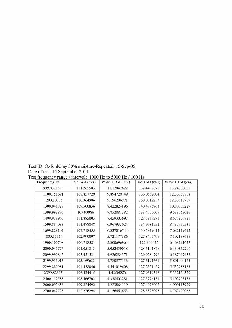
30
Test ID: OxfordClay 30% moisture-Repeated, 15-Sep-05 Date of test: 15 September 2011 Test frequency range / interval: 1000 Hz to 5000 Hz / 100 Hz
Frequency(Hz) Vel A-B(m/s) Wave L A-B (cm) Vel C-D (m/s) Wave L C-D(cm)
999.8321533 111.265583 11.12842622 132.4457678 13.24680021
1100.158691 108.857729 9.894729749 136.0532004 12.36668868
1200.10376 110.364986 9.196286971 150.0512253 12.50318767
1300.048828 109.500836 8.422824896 140.4875963 10.80633229
1399.993896 109.93986 7.852881382 133.4707005 9.533663026
1499.938965 111.885003 7.459303697 128.5938281 8.573270721
1599.884033 111.478848 6.967933024 134.9981752 8.437997531
1699.829102 107.718455 6.337016744 130.5829014 7.682119412
1800.15564 102.990097 5.721177386 127.8495496 7.102138658
1900.100708 100.718581 5.300696964 122.904055 6.468291627
2000.045776 101.051313 5.052450018 128.6101878 6.430362209
2099.990845 103.451521 4.926284371 129.9284796 6.187097432
2199.935913 105.169633 4.780577136 127.6191661 5.801040175
2299.880981 104.438046 4.541019608 127.2521429 5.532988183
2399.82605 106.434415 4.43508876 127.9619546 5.332134579
2500.152588 108.466702 4.338403281 127.5776151 5.102793153
2600.097656 109.824592 4.223864119 127.4078007 4.900115979
2700.042725 112.226294 4.156463653 128.5895095 4.762499066

31
2799.987793 113.15516 4.041273338 129.9972073 4.642777644
2899.932861 114.092235 3.934306096 132.1883266 4.558323688
2999.87793 115.897438 3.863405151 134.0347456 4.468006657
3099.822998 118.182644 3.81256105 135.4924829 4.370974828
3200.149536 119.671482 3.739559051 137.0529312 4.282703968
3300.094604 120.15673 3.641008643 138.5208514 4.197481224
3400.039673 119.444375 3.513028873 138.5522361 4.075018219
3499.984741 119.654431 3.418712922 138.6102927 3.960311344
3599.92981 118.243047 3.284593127 142.3055586 3.953009257
3699.874878 116.521326 3.149331525 143.8278475 3.887370579
3799.819946 116.56014 3.067517443 143.9090818 3.787260551
3900.146484 116.606869 2.989807431 144.6509225 3.708858708
4000.091553 115.979357 2.899417555 144.218241 3.605373506
4100.036621 117.936459 2.876473301 144.1011263 3.514630224
4199.981689 139.818968 3.329037552 143.9966023 3.428505477
4299.926758 140.805448 3.274601084 143.8878819 3.34628681
4399.871826 132.118339 3.002776995 142.1173657 3.230034222
4499.816895 126.586724 2.813152789 139.0987906 3.091210017
4600.143433 124.674977 2.710241077 135.671789 2.949294756
4700.088501 123.577719 2.629263656 137.2890032 2.920987619
4800.033569 122.288924 2.547668091 139.2373198 2.900757209
4899.978638 122.0031 2.489870036 140.3951521 2.865219677
4999.923706 122.055811 2.441153472 140.9169246 2.818381497
frequency (Hz) Surface Vel A-B (m/s)
Shear wave Vel A-B (m/s)
Vs2 (m/s)
G(kg/ms2), N/m2
G (Mpa)
999.8322 111.2656 116.4951 13571.1 23613715 23.61371
1100.159 108.8577 113.974 12990.08 22602743 22.60274
1200.104 110.365 115.5521 13352.3 23232997 23.233
1300.049 109.5008 114.6474 13144.02 22870596 22.8706
1399.994 109.9399 115.107 13249.63 23054355 23.05435
1499.939 111.885 117.1436 13722.62 23877363 23.87736
1599.884 111.4788 116.7184 13623.17 23704323 23.70432
1699.829 107.7185 112.7812 12719.6 22132111 22.13211
1800.156 102.9901 107.8306 11627.45 20231755 20.23175
1900.101 100.7186 105.4524 11120.2 19349146 19.34915
2000.046 101.0513 105.8007 11193.79 19477201 19.4772
2099.991 103.4515 108.3137 11731.87 20413448 20.41345
2199.936 105.1696 110.1126 12124.79 21097128 21.09713
2299.881 104.438 109.3466 11956.69 20804634 20.80463
2399.826 106.4344 111.4368 12418.17 21607612 21.60761
2500.153 108.4667 113.5646 12896.93 22440653 22.44065
2600.098 109.8246 114.9863 13221.86 23006037 23.00604
2700.043 112.2263 117.5009 13806.47 24023255 24.02326

32
2799.988 113.1552 118.4735 14035.96 24422569 24.42257
2899.933 114.0922 119.4546 14269.39 24828746 24.82875
2999.878 115.8974 121.3446 14724.52 25620658 25.62066
3099.823 118.1826 123.7372 15310.9 26640969 26.64097
3200.15 119.6715 125.296 15699.1 27316430 27.31643
3300.095 120.1567 125.8041 15826.67 27538407 27.53841
3400.04 119.4444 125.0583 15639.57 27212849 27.21285
3499.985 119.6544 125.2782 15694.62 27308647 27.30865
3599.93 118.243 123.8005 15326.56 26668208 26.66821
3699.875 116.5213 121.9978 14883.47 25897238 25.89724
3799.82 116.5601 122.0385 14893.39 25914494 25.91449
3900.146 116.6069 122.0874 14905.33 25935277 25.93528
4000.092 115.9794 121.4304 14745.34 25656889 25.65689
4100.037 117.9365 123.4795 15247.18 26530093 26.53009
4199.982 139.819 146.3905 21430.17 37288490 37.28849
4299.927 140.8054 147.4233 21733.63 37816517 37.81652
4399.872 132.1183 138.3279 19134.61 33294218 33.29422
4499.817 126.5867 132.5363 17565.87 30564615 30.56462
4600.143 124.675 130.5347 17039.31 29648396 29.6484
4700.089 123.5777 129.3859 16740.7 29128825 29.12882
4800.034 122.2889 128.0365 16393.35 28524422 28.52442
4899.979 122.0031 127.7372 16316.8 28391239 28.39124
4999.924 122.0558 127.7924 16330.91 28415777 28.41578
frequency (Hz) Surface Vel C-D (m/s)
Shear wave Vel C-D (m/s)
Vs2 (m/s)
G(kg/ms2), N/m2
G (Mpa)
999.8322 132.4458 138.6707 19229.57 33459449 33.45945
1100.159 136.0532 142.4477 20291.35 35306945 35.30694
1200.104 150.0512 157.1036 24681.55 42945900 42.9459
1300.049 140.4876 147.0905 21635.62 37645977 37.64598
1399.994 133.4707 139.7438 19528.34 33979305 33.9793
1499.939 128.5938 134.6377 18127.32 31541538 31.54154
1599.884 134.9982 141.3431 19977.87 34761492 34.76149
1699.829 130.5829 136.7203 18692.44 32524845 32.52485
1800.156 127.8495 133.8585 17918.09 31177481 31.17748
1900.101 122.9041 128.6805 16558.68 28812108 28.81211
2000.046 128.6102 134.6549 18131.93 31549564 31.54956
2099.991 129.9285 136.0351 18505.55 32199663 32.19966
2199.936 127.6192 133.6173 17853.57 31065219 31.06522
2299.881 127.2521 133.233 17751.03 30886793 30.88679
2399.826 127.962 133.9762 17949.61 31232327 31.23233
2500.153 127.5776 133.5738 17841.95 31044993 31.04499
2600.098 127.4078 133.396 17794.48 30962402 30.9624

33
2700.043 128.5895 134.6332 18126.1 31539419 31.53942
2799.988 129.9972 136.1071 18525.14 32233737 32.23374
2899.933 132.1883 138.4012 19154.89 33329502 33.3295
2999.878 134.0347 140.3344 19693.74 34267104 34.2671
3099.823 135.4925 141.8606 20124.44 35016523 35.01652
3200.15 137.0529 143.4944 20590.65 35827728 35.82773
3300.095 138.5209 145.0313 21034.09 36599312 36.59931
3400.04 138.5522 145.0642 21043.62 36615898 36.6159
3499.985 138.6103 145.125 21061.26 36646590 36.64659
3599.93 142.3056 148.9939 22199.19 38626587 38.62659
3699.875 143.8278 150.5878 22676.67 39457410 39.45741
3799.82 143.9091 150.6728 22702.3 39501994 39.50199
3900.146 144.6509 151.4495 22936.96 39910303 39.9103
4000.092 144.2182 150.9965 22799.94 39671900 39.6719
4100.037 144.1011 150.8739 22762.93 39607494 39.60749
4199.982 143.9966 150.7644 22729.92 39550056 39.55006
4299.927 143.8879 150.6506 22695.61 39490356 39.49036
4399.872 142.1174 148.7969 22140.51 38524491 38.52449
4499.817 139.0988 145.6364 21209.97 36905349 36.90535
4600.143 135.6718 142.0484 20177.74 35109263 35.10926
4700.089 137.289 143.7416 20661.64 35951260 35.95126
4800.034 139.2373 145.7815 21252.24 36978894 36.97889
4899.979 140.3952 146.9937 21607.15 37596450 37.59645
4999.924 140.9169 147.54 21768.06 37876420 37.87642
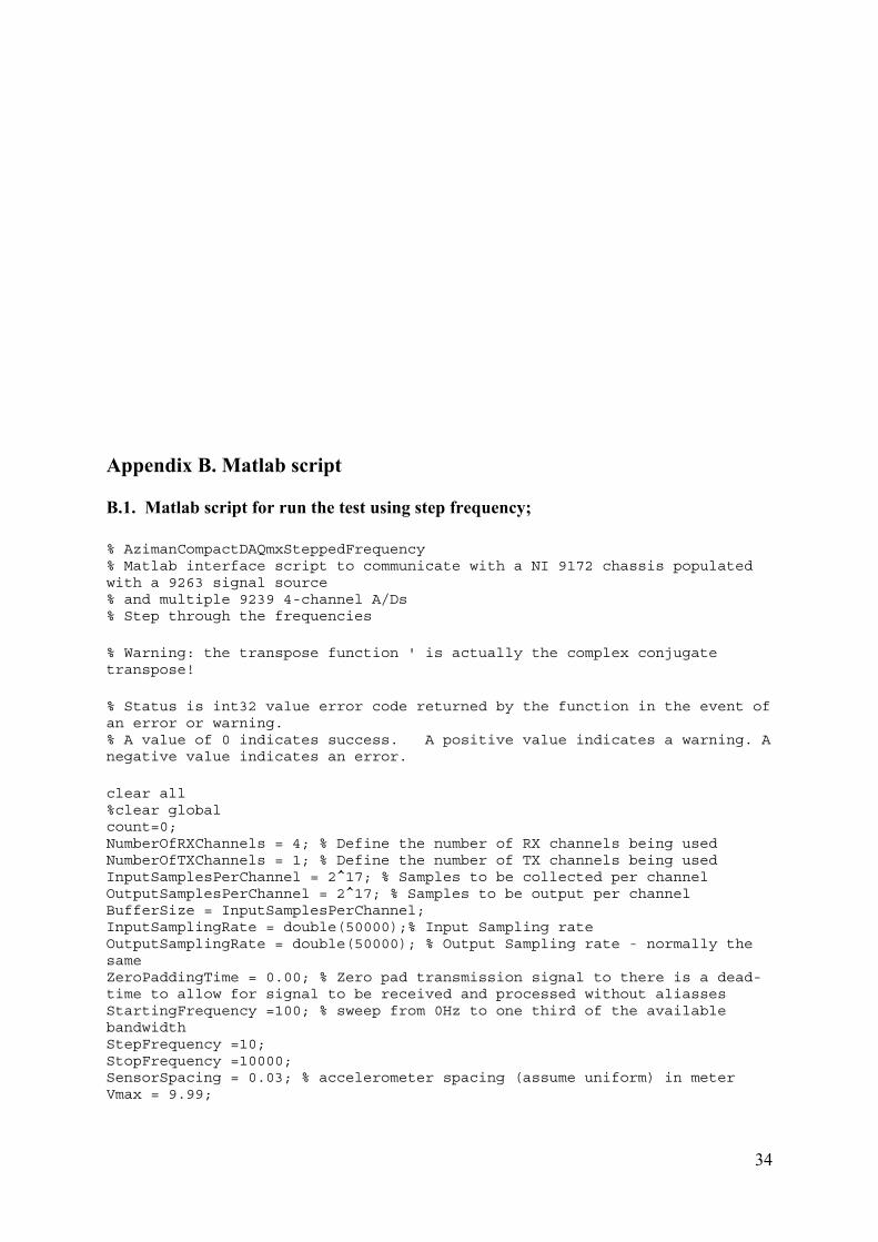
34
Appendix B. Matlab script B.1. Matlab script for run the test using step frequency; % AzimanCompactDAQmxSteppedFrequency % Matlab interface script to communicate with a NI 9172 chassis populated with a 9263 signal source % and multiple 9239 4-channel A/Ds % Step through the frequencies % Warning: the transpose function ' is actually the complex conjugate transpose! % Status is int32 value error code returned by the function in the event of an error or warning. % A value of 0 indicates success. A positive value indicates a warning. A negative value indicates an error. clear all %clear global count=0; NumberOfRXChannels = 4; % Define the number of RX channels being used NumberOfTXChannels = 1; % Define the number of TX channels being used InputSamplesPerChannel = 2^17; % Samples to be collected per channel OutputSamplesPerChannel = 2^17; % Samples to be output per channel BufferSize = InputSamplesPerChannel; InputSamplingRate = double(50000);% Input Sampling rate OutputSamplingRate = double(50000); % Output Sampling rate - normally the same ZeroPaddingTime = 0.00; % Zero pad transmission signal to there is a dead-time to allow for signal to be received and processed without aliasses StartingFrequency =100; % sweep from 0Hz to one third of the available bandwidth StepFrequency =10; StopFrequency =10000; SensorSpacing = 0.03; % accelerometer spacing (assume uniform) in meter Vmax = 9.99;

35
NumOfPhaseRotation=1; EstimatedVelocity=50; LoopThroughTest = 0; % Test delay from transmit to receive CrossSpectrumMeasurements = 1;% Collect data for velocity/phase coherence measurements NumberOfSnapshots =5; % Number of data collection operations to measure real data PassBandFraction = 0.50; % A/D converter passband as a ratio of the sampling frequency Bandwidth = OutputSamplingRate*PassBandFraction; % Bandwidth of transmission signal % Add experiment information here Comment1 = 'One current measuring channel and four accelerometer. Order from Department: REF,Chan1,Chan2...Chan4'; Comment2 = 'Chan0 measures voltage across 10 0hm resistor, Chans 1 - 4 measure voltage from accelerometers'; Comment3 = 'Add specific comments here'; % Check out valid sampling rate ValidSamplingRates = 50e3./(1:31); % Search for best fit of sampling rate [ActualInputSamplingRate ActualInputSamplingRateIndex] = min(abs(InputSamplingRate-ValidSamplingRates)); ActualInputSamplingRate = ValidSamplingRates(ActualInputSamplingRateIndex); if ActualInputSamplingRate~=InputSamplingRate, fprintf('Program input sampling rate replaced with actual sampling rate of %f Hz\n',ActualInputSamplingRate); InputSamplingRate = ActualInputSamplingRate; end [ActualOutputSamplingRate ActualOutputSamplingRateIndex] = min(abs(OutputSamplingRate-ValidSamplingRates)); ActualOutputSamplingRate = ValidSamplingRates(ActualOutputSamplingRateIndex); if ActualOutputSamplingRate~=OutputSamplingRate, fprintf('Program output sampling rate replaced with actual sampling rate of %f Hz\n',ActualOutputSamplingRate); OutputSamplingRate = ActualOutputSamplingRate; end fprintf('Observation period = %f s\n',InputSamplesPerChannel/ActualOutputSamplingRate); % Predicted input A/D channel latency PredictedInputLatency = 38.4/InputSamplingRate + 3e-6; % latency measured in seconds % Predict output D/A latency OutputLatency = [3e-6 5e-6 7.5e-6 9.5e-6]; PredictedOutputLatency = OutputLatency(NumberOfTXChannels); % Measurements imply an extra few samples of delay AdditionalDelaySamples = 2; TotalPredictedLatency = PredictedOutputLatency + PredictedInputLatency + AdditionalDelaySamples/InputSamplingRate + 1.8e-6;
36
% The IDAQmx DLL functions appear to exist in 'nicaiu.dll' if ~libisloaded('nicaiu') % checks if library is loaded %hfile = 'C:\Program Files\National Instruments\NI-DAQ\DAQmx ANSI C Dev\include\NIDAQmx.h'; %hfile = 'C:\\Program Files\\National Instruments\\NI-DAQ\\DAQmx ANSI C Dev\\include\\NIDAQmx.h'; hfile = 'NIDAQmx.h'; [notfound,warnings] = loadlibrary('nicaiu.dll', hfile, 'mfilename', 'mxproto'); % mxproto contains the function prototypes end %% required constants (see NIDAQmx.h) % Terminal Configuration DAQmx_Val_Cfg_Default = int32(-1); % Default DAQmx_Val_RSE = int32(10083); % RSE DAQmx_Val_NRSE = int32(10078); % NRSE DAQmx_Val_Diff = int32(10106); % Differential DAQmx_Val_PseudoDiff = int32(12529); % Pseudodifferential
% Units DAQmx_Val_Volts = int32(10348); % Volts DAQmx_Val_FromCustomScale = int32(10065); % From Custom Scale
% Active Edge DAQmx_Val_Rising = int32(10280); % Rising DAQmx_Val_Falling = int32(10171); % Falling
% Sample Mode DAQmx_Val_FiniteSamps = int32(10178); % Finite Samples DAQmx_Val_ContSamps = int32(10123); % Continuous Samples DAQmx_Val_HWTimedSinglePoint = int32(12522); % Hardware Timed Single Point
% Fill Mode DAQmx_Val_GroupByChannel = uint32(0); % Group by Channel DAQmx_Val_GroupByScanNumber = uint32(1); % Group by Scan Number
% Device ID DAQmx_Val_CompactDAQChassis = uint32(14658); % CompactDAQ chassis %% Try getting names of NI cards DeviceNames = libpointer('stringPtr',blanks(60)); [Status, DeviceNames] = calllib('nicaiu','DAQmxGetSysDevNames',DeviceNames,uint32(60)); %DAQmxGetSysDevNames(char *data, uInt32 bufferSize); if isempty(DeviceNames), fprintf('No NI DAQ devices found\n'); unloadlibrary 'nicaiu'; % unload library return end % There may be multiple device in a comma-separated list CommaSeparatedVariableCell = textscan(DeviceNames, '%s', 'delimiter', ','); % Convert to a list of CSV names % Process each name in-turn IndividualDeviceNameList = cell(numel(CommaSeparatedVariableCell1),1); for DeviceNameIndex = 1:numel(CommaSeparatedVariableCell1), IndividualDeviceName = char(CommaSeparatedVariableCell1(DeviceNameIndex)); fprintf('Device Name = %s ',IndividualDeviceName); ProductType = libpointer('stringPtr',blanks(60));

37
[Status,IndividualDeviceName,ProductType] = calllib('nicaiu','DAQmxGetDevProductType',IndividualDeviceName,ProductType,uint32(60)); %int32 DAQmxGetDevProductType(const char device[], char *data, uInt32 bufferSize); IndividualDeviceNameListDeviceNameIndex,1 = char(ProductType); fprintf('Product Type = %s\n',ProductType); end % Check if required chassis exists in list DeviceComparison = strcmp(IndividualDeviceNameList,'cDAQ-9172'); if sum(DeviceComparison) == 0, fprintf('cDAQ-9172 compact device chassis not found\n'); unloadlibrary 'nicaiu'; % unload library return end % Recover device name of chassis IndividualChassisName = char(CommaSeparatedVariableCell1(DeviceComparison)); % Check if required input modules exists in list DeviceComparison = strcmp(IndividualDeviceNameList,'NI 9239'); if sum(DeviceComparison) == 0, fprintf('No NI 9239 A/D modules found\n'); unloadlibrary 'nicaiu'; % unload library return end % Recover device name of A/D modules IndividualADNames = char(CommaSeparatedVariableCell1(DeviceComparison)); % Check if required output modules exists in list DeviceComparison = strcmp(IndividualDeviceNameList,'NI 9263'); if sum(DeviceComparison) == 0, fprintf('No NI 9263 D/A modules found\n'); unloadlibrary 'nicaiu'; % unload library return end % Recover device name of D/A modules IndividualDANames = char(CommaSeparatedVariableCell1(DeviceComparison)); %% Determine which input channels are available in device - there may be multiple modules for ModuleIndex = 1:size(IndividualADNames,1), PhysicalChannels = libpointer('stringPtr',blanks(200)); [Status,IndividualDeviceName,PhysicalChannels] = calllib('nicaiu','DAQmxGetDevAIPhysicalChans',IndividualADNames(ModuleIndex,:),PhysicalChannels,uint32(200)); %int32 DAQmxGetDevAIPhysicalChans(const char device[], char *data, uInt32 bufferSize); if Status ~= 0, fprintf('Error in DAQmxGetDevAIPhysicalChans. Status = %d\n',Status); return end % There may be multiple physical channels in a comma-separated list CommaSeparatedVariableCell = textscan(PhysicalChannels, '%s', 'delimiter', ','); % Convert to a list of CSV names % Convert to a full list if ModuleIndex == 1,

38
IndividualPhysicalChannelName = cell(numel(CommaSeparatedVariableCell1),size(IndividualADNames,1)); end for PhysicalChannelIndex = 1:numel(CommaSeparatedVariableCell1), IndividualPhysicalChannelNamePhysicalChannelIndex,ModuleIndex = char(CommaSeparatedVariableCell1(PhysicalChannelIndex)); end end %% Analogue Input configuration string generation % Make a single string determined by the 'NumberOfRXChannels' requested if NumberOfRXChannels > numel(IndividualPhysicalChannelName), fprintf('Request number of A/D channels exceeds the number available\n'); return end % Assume A/D modules are obtained in groups of four CompleteADModules = floor((NumberOfRXChannels-1)/4); % e.g. 0,0,0,0,1,1,1,1,2,2,2,2,3,3,3,3 PartialADChannels = mod((NumberOfRXChannels-1),4); % e.g. 1,2,3,4,1,2,3,4,1,2,3,4,1,2,3,4 if NumberOfRXChannels == 1, % single channel AIConfigString =IndividualPhysicalChannelName1,1; else % multiple channels AIConfigString = ''; if CompleteADModules >= 1, for ModulesIndex = 1:CompleteADModules, % Complete group of four channels AIConfigString = strcat(AIConfigString,cellstr([IndividualPhysicalChannelName1,ModulesIndex ':' IndividualPhysicalChannelName4,ModulesIndex]),','); end end % Add in last group if PartialADChannels == 0, AIConfigString = strcat(AIConfigString,IndividualPhysicalChannelName1,CompleteADModules+1,','); else AIConfigString = strcat(AIConfigString,cellstr([IndividualPhysicalChannelName1,CompleteADModules+1 ':' IndividualPhysicalChannelNamePartialADChannels+1,CompleteADModules+1])); end end AIConfigString = char(AIConfigString); fprintf('A/D Configuration String = %s\n',AIConfigString); %% Determine which output channels are available in device - there may be multiple modules for ModuleIndex = 1:size(IndividualDANames,1), PhysicalChannels = libpointer('stringPtr',blanks(200)); [Status,IndividualDeviceName,PhysicalChannels] = calllib('nicaiu','DAQmxGetDevAOPhysicalChans',IndividualDANames(ModuleIndex,:),PhysicalChannels,uint32(200));
39
%int32 DAQmxGetDevAIPhysicalChans(const char device[], char *data, uInt32 bufferSize); if Status ~= 0, fprintf('Error in DAQmxGetDevAOPhysicalChans. Status = %d\n',Status); return end % There may be multiple physical channels in a comma-separated list CommaSeparatedVariableCell = textscan(PhysicalChannels, '%s', 'delimiter', ','); % Convert to a list of CSV names % Convert to a full list if ModuleIndex == 1, IndividualPhysicalChannelName = cell(numel(CommaSeparatedVariableCell1),size(IndividualDANames,1)); end for PhysicalChannelIndex = 1:numel(CommaSeparatedVariableCell1), IndividualPhysicalChannelNamePhysicalChannelIndex,ModuleIndex = char(CommaSeparatedVariableCell1(PhysicalChannelIndex)); end end % Re-arrange into a single row vector IndividualPhysicalChannelName = reshape(IndividualPhysicalChannelName,[],1); %% Analogue Output configuration string generation % Make a single string determined by the 'NumberOfTXChannels' requested if NumberOfTXChannels > numel(IndividualPhysicalChannelName), fprintf('Request number of D/a channels exceeds the number available\n'); return end % Assume D/A modules are obtained in groups of four CompleteDAModules = floor((NumberOfTXChannels-1)/4); % e.g. 0,0,0,0,1,1,1,1,2,2,2,2,3,3,3,3 PartialDAChannels = mod((NumberOfTXChannels-1),4); % e.g. 1,2,3,4,1,2,3,4,1,2,3,4,1,2,3,4 if NumberOfTXChannels == 1, % single channel AOConfigString =IndividualPhysicalChannelName1,1; else % multiple channels AOConfigString = ''; if CompleteDAModules >= 1, for ModulesIndex = 1:CompleteDAModules, % Complete group of four channels AOConfigString = strcat(AOConfigString,cellstr([IndividualPhysicalChannelName1,ModulesIndex ':' IndividualPhysicalChannelName4,ModulesIndex]),','); end end % Add in last group if PartialDAChannels == 0, AOConfigString = strcat(AOConfigString,IndividualPhysicalChannelName1,CompleteDAModules+1,','); else

40
AOConfigString = strcat(AOConfigString,cellstr([IndividualPhysicalChannelName1,CompleteDAModules+1 ':' IndividualPhysicalChannelNamePartialDAChannels+1,CompleteDAModules+1])); end end AOConfigString = char(AOConfigString); fprintf('D/A Configuration String = %s\n',AOConfigString); %% Create new tasks TaskHandle1 = libpointer('uint32Ptr',0); % VOID task handle pointers TaskHandle2 = libpointer('uint32Ptr',0); InputTaskName = 'AITask'; OutputTaskName = 'AOTask'; [Status,TaskNameText,TaskHandle1] = calllib('nicaiu','DAQmxCreateTask',InputTaskName,TaskHandle1); % Create a NIDAQmx Task TaskHandle1 % int32 DAQmxCreateTask (const char taskName[], TaskHandle, *taskHandle); if Status ~= 0, fprintf('Error in DAQmxCreateTask - Input Task. Status = %d\n',Status); return end TaskHandle1Numeric = TaskHandle1; TaskHandle1 = libpointer('uint32Ptr',TaskHandle1); [Status,TaskNameText,TaskHandle2] = calllib('nicaiu','DAQmxCreateTask',OutputTaskName,TaskHandle2); % Create a NIDAQmx Task TaskHandle2 % int32 DAQmxCreateTask (const char taskName[], TaskHandle, *taskHandle); if Status ~= 0, fprintf('Error in DAQmxCreateTask - Output Task. Status = %d\n',Status); return end TaskHandle2Numeric = TaskHandle2; TaskHandle2 = libpointer('uint32Ptr',TaskHandle2); % Generate a D/A output channels and A/D input channel to be referred to % later minVal = double(-10); maxVal = double(10); % Generate a D/A output channel [Status,ChannelNameText,c,d] = calllib('nicaiu','DAQmxCreateAOVoltageChan',TaskHandle2Numeric,AOConfigString,'',minVal,maxVal,DAQmx_Val_Volts,''); % int32 DAQmxCreateAOVoltageChan (TaskHandle taskHandle, const char physicalChannel[], const char nameToAssignToChannel[], float64 minVal, float64 maxVal, int32 units, const char customScaleName[]); if Status ~= 0, fprintf('Error in DAQmxCreateAOVoltageChan. Status = %d\n',Status); return end [Status,ChannelNameText,c,d] = calllib('nicaiu','DAQmxCreateAIVoltageChan',TaskHandle1Numeric,AIConfigString,'',DAQmx_Val_Diff,minVal,maxVal,DAQmx_Val_Volts,'');
41
% int32 DAQmxCreateAIVoltageChan (TaskHandle taskHandle, const char physicalChannel[], const char nameToAssignToChannel[], % int32 terminalConfig, float64 minVal, float64 maxVal, int32 units, const char customScaleName[]); if Status ~= 0, fprintf('Error in DAQmxCreateAIVoltageChan. Status = %d\n',Status); return end %% % Set up the on-board timing with internal clock source ActiveEdge = DAQmx_Val_Rising; % Samplig edge SampleMode = DAQmx_Val_FiniteSamps; % Collect a finite number of samples %SampleMode = DAQmx_Val_ContSamps; % Collect samples continuously %SamplesToAcquire = uint64(InputSamplesPerChannel*NumberOfRXChannels); % Make buffer size large - several times expected window size SamplesToAcquire = uint64(BufferSize); [Status,ClockSource] = calllib('nicaiu','DAQmxCfgSampClkTiming',TaskHandle1Numeric,'OnboardClock',InputSamplingRate,ActiveEdge,SampleMode,SamplesToAcquire); % int32 DAQmxCfgSampClkTiming (TaskHandle taskHandle, const char source[],float64 rate, int32 ActiveEdge, int32 SampleMode, uInt64 % sampsPerChanToAcquire); if Status ~= 0, fprintf('Error in DAQmxCfgSampClkTiming for TaskHandle1 Status = %d\n',Status); Status = calllib('nicaiu','DAQmxClearTask',TaskHandle1); % Clear the task return end TerminalName = 'ai/StartTrigger'; % Define the parameters for a digital edge start trigger for output. Set the analog output to trigger off the AI start trigger. This is an internal trigger signal. [Status,a] = calllib('nicaiu','DAQmxCfgDigEdgeStartTrig',TaskHandle2Numeric,TerminalName,DAQmx_Val_Rising); % [int32] DAQmxCfgDigEdgeStartTrig (TaskHandle taskHandle, const char triggerSource[], int32 triggerEdge); if Status ~= 0, fprintf('Error in DAQmxCfgDigEdgeStartTrig. Status = %d\n',Status); Status = calllib('nicaiu','DAQmxClearTask',TaskHandle2Numeric); % Clear the task return end %% Make an LFM transmission signal ZeroPaddingPoints = round(OutputSamplingRate.*ZeroPaddingTime); % This is the number of zeros to be added after the transmission has finished ActiveTXPoints = OutputSamplesPerChannel - ZeroPaddingPoints; % This is the number of samples within the active region of the TX signal % Weight received signals with a suitable window WeightingFunction = tukeywin(ActiveTXPoints,0.005)'; % Tukey Window
42
% Make a single chirp signal for transmission % Make a complex chirp signal - zero padded TXSignal = zeros(1,OutputSamplesPerChannel); TXTimeIndex = 0:ActiveTXPoints-1; %TXSignal(1,1:ActiveTXPoints) = exp(j.*(StartingFrequency*2*pi*TXTimeIndex/OutputSamplingRate + Bandwidth*2*pi*TXTimeIndex.^2./(2*ActiveTXPoints*OutputSamplingRate))); FixedFrequency = 500; TXSignal(1,1:ActiveTXPoints) = exp(j.*(FixedFrequency*2*pi*TXTimeIndex/OutputSamplingRate)); % scale result TXSignal(1:ActiveTXPoints) = Vmax .* WeightingFunction.*TXSignal(1:ActiveTXPoints) / max(abs(TXSignal)); TXSignal('last') = 0; % Last sample should be zero % Make a one-sided spectral estimate of the complex TX signal - including zero padding DriveFFT2N = conj(fft(TXSignal,2*InputSamplesPerChannel) ./ InputSamplesPerChannel); % If the signal was generated in a complex form then convert back to a real number if ~isreal(TXSignal), % Convert back to a real signal (start at zero voltage) TXSignal = -imag(TXSignal); end % Calculate the spectrum of the transmitted signal TXSignalFFT = conj(fft(TXSignal)); % Time index for display purposes TimeIndex = (0:(OutputSamplesPerChannel-1))/OutputSamplingRate; % Frequency index for display purposes - assuming zero padded FrequencyIndex = (0:(OutputSamplesPerChannel -1)).*OutputSamplingRate./OutputSamplesPerChannel; DisplayThis = 0; if DisplayThis == 1, figure(1) plot(TimeIndex,real(TXSignal),'r') title('Transmitted waveform') xlabel('Time (s)') ylabel('Voltage (V)') figure(2) plot(FrequencyIndex,20*log10(abs(fft(TXSignal)./OutputSamplesPerChannel))); title('Spectrum of transmitted signal') xlabel('Frequency (Hz)') ylabel('Spectrum Level (dB)') xlim([0 OutputSamplingRate*PassBandFraction]) end %% % Make buffer size same as number of samples transmitted - SamplesToTx = uint64(BufferSize);
43
[Status,ClockSource] = calllib('nicaiu','DAQmxCfgSampClkTiming',TaskHandle2Numeric,'ai/SampleClock',OutputSamplingRate,ActiveEdge,SampleMode,SamplesToTx); if Status ~= 0, fprintf('Error in DAQmxCfgSampClkTiming for TaskHandle2. Status = %d\n',Status); Status = calllib('nicaiu','DAQmxClearTask',TaskHandle2Numeric); % Clear the task return end %% LoopThroughLatency = zeros(1,NumberOfRXChannels); if LoopThroughTest == 1, %% Write samples to task SamplesPerChannelWritten = libpointer('int32Ptr',0); [Status,DAQmxWriteAnalogF64Return1,DAQmxWriteAnalogF64Return2] = calllib('nicaiu','DAQmxWriteAnalogF64',TaskHandle2Numeric,int32(OutputSamplesPerChannel),int32(0),double(-1),DAQmx_Val_GroupByScanNumber,TXSignal,SamplesPerChannelWritten,[]); % int32 DAQmxWriteAnalogF64 (TaskHandle taskHandle, int32 numSampsPerChan, bool32 autoStart, float64 timeout, bool32 dataLayout, float64 writeArray[], int32 *sampsPerChanWritten, bool32 *reserved); if Status ~= 0, fprintf('Error in DAQmxWriteAnalogF64. Status = %d\n',Status); Status = calllib('nicaiu','DAQmxClearTask',TaskHandle1Numeric); %#ok<NASGU> % Clear the tasks Status = calllib('nicaiu','DAQmxClearTask',TaskHandle2Numeric); return end % Perform loop-through latency check for InputSensorIndex = 1:NumberOfRXChannels, % Scan through each input channel % Prompt user to connect desired loop through fprintf('Testing input channel %d\n',InputSensorIndex-1) UserReply = input('Connect output to desired input channel and press enter','s'); % Collect data % Start the tasks - start output before input as the input task would trigger the output task Status = calllib('nicaiu','DAQmxStartTask',TaskHandle2Numeric); % int32 DAQmxStartTask (TaskHandle taskHandle); if Status ~= 0, fprintf('Error in DAQmxStartTask. Status = %d\n',Status); Status = calllib('nicaiu','DAQmxClearTask',TaskHandle2Numeric); % Clear the task return end Status = calllib('nicaiu','DAQmxStartTask',TaskHandle1Numeric); % int32 DAQmxStartTask (TaskHandle taskHandle); if Status ~= 0, fprintf('Error in DAQmxStartTask. Status = %d\n',Status); Status = calllib('nicaiu','DAQmxClearTask',TaskHandle1Numeric); %#ok<NASGU> % Clear the tasks Status = calllib('nicaiu','DAQmxClearTask',TaskHandle2Numeric); return end %FillMode = DAQmx_Val_GroupByChannel;

44
FillMode = DAQmx_Val_GroupByScanNumber; % Interleaved samples RecoveredInputData = zeros(InputSamplesPerChannel*NumberOfRXChannels,1); Timeout = double(-1); % maximum waiting time before timeout (in secs) RecoveredInputDataPtr = libpointer('doublePtr',zeros(InputSamplesPerChannel*NumberOfRXChannels,1)); ReadPtr = libpointer('int32Ptr',0); ReservedPtr = libpointer('uint32Ptr',[]); [Status,RecoveredData,DAQmxReadAnalogF64Return1,DAQmxReadAnalogF64Return2] = calllib('nicaiu','DAQmxReadAnalogF64',TaskHandle1Numeric,int32(InputSamplesPerChannel),Timeout,FillMode,RecoveredInputDataPtr,uint32(InputSamplesPerChannel*NumberOfRXChannels),ReadPtr,ReservedPtr); % int32 DAQmxReadAnalogF64 (TaskHandle taskHandle, int32 numSampsPerChan, float64 timeout, bool32 fillMode, float64 readArray[], uInt32 arraySizeInSamps,int32 *sampsPerChanRead, bool32 *reserved); if Status ~= 0, fprintf('Error in DAQmxReadAnalogF64. Status = %d\n',Status); end % Stop the tasks Status = calllib('nicaiu','DAQmxStopTask',TaskHandle1Numeric); % int32 DAQmxStopTask(uint32) % int32 DAQmxStopTask (TaskHandle taskHandle); if Status ~= 0, fprintf('Error/warning in DAQmxStopTask. Status = %d\n',Status); end Status = calllib('nicaiu','DAQmxStopTask',TaskHandle2Numeric); if Status ~= 0, fprintf('Error/warning in DAQmxStopTask. Status = %d\n',Status); end % If more than one A/D channel is used, then the sampes should be separated RecoveredData = reshape(RecoveredData,NumberOfRXChannels,InputSamplesPerChannel); figure(3) plot(TimeIndex,RecoveredData(InputSensorIndex,:)) title('Raw Input Data') xlabel('Time (s)') ylabel('Voltage (V)') ylim([-1 1]) RecoveredDataFFT = fft(RecoveredData(InputSensorIndex,:),2*InputSamplesPerChannel); % Calculate the covariance RecoveredDataFFT(1) = 0; % Remove any DC component DisplayThis = 1; if DisplayThis == 1, figure(4)

45
PaddedFrequencyIndex = (0:(2*OutputSamplesPerChannel -1)).*OutputSamplingRate/OutputSamplesPerChannel/2; plot(PaddedFrequencyIndex,20*log10(abs(DriveFFT2N)),'r') hold on plot(PaddedFrequencyIndex,20*log10(abs(RecoveredDataFFT) ./ InputSamplesPerChannel),'k'); hold off legend('Drive Signal','Sense Signal',0) ylabel('Spectral Amplitude (dB)') xlabel('Frequency (Hz)') title('Linear Spectra of Transmit and Received Signals'); xlim([0 InputSamplingRate*PassBandFraction]); drawnow end % Calculate the correlation function CrossSpectrum = RecoveredDataFFT .* DriveFFT2N; CrossCorrelation = ifft(CrossSpectrum); [maxval LoopThroughLatency(InputSensorIndex)] = max(abs(CrossCorrelation)); % Re-order data - swap frequency portions %CrossCorrelation = [CrossCorrelation(NumberSamples+1:2*NumberSamples) ; CrossCorrelation(1:NumberSamples)]; figure(5) DisplayTimeIndex2N = (0:(2*InputSamplesPerChannel-1))/InputSamplingRate; plot(DisplayTimeIndex2N,abs(CrossCorrelation),'k') title('Cross Correlation Function') ylabel('Magnitude') xlabel('Time (s)') %xlim([0 RXSamplingFrequency/(2*NumberRXChannels)]) drawnow % select a small bit of the correlation output SegmentLength = 1000; SegmentCrossCorrelation = CrossCorrelation(1:SegmentLength); SegmentCrossCorrelation = abs(SegmentCrossCorrelation); SegmentTime = DisplayTimeIndex2N(1:SegmentLength); % Normalise correlation value SegmentCrossCorrelation = SegmentCrossCorrelation ./ max(SegmentCrossCorrelation); figure(6) plot(SegmentTime,SegmentCrossCorrelation,'k') title('Cross Correlation Function') ylabel('Magnitude') xlabel('Time (s)') % Plot the cross spectrum % First correct by the guess DisplayFrequencyIndex2N = InputSamplingRate*(0:(2*InputSamplesPerChannel-1))/(2*InputSamplesPerChannel); CompensationFunction = exp(j*2*pi*DisplayFrequencyIndex2N*TotalPredictedLatency); CompensatedCrossSpectrum = CompensationFunction .* CrossSpectrum; figure(7) plot(DisplayFrequencyIndex2N/1000,angle(CrossSpectrum),DisplayFrequencyIndex2N/1000,angle(CompensatedCrossSpectrum))
46
title('Cross Spectrum Function') ylabel('Phase (rads)') xlabel('Frequency (kHz)') figure(8) plot(DisplayFrequencyIndex2N/1000,abs(CrossSpectrum)) title('Cross Spectrum Function') ylabel('Magnitude)') xlabel('Frequency (kHz)') %xlim([0 RXSamplingFrequency/(2*NumberRXChannels)]) drawnow end % Convert sample values into time LoopThroughLatencyTime = DisplayTimeIndex2N(LoopThroughLatency); fprintf('Measured Latency = %e secs \n',LoopThroughLatencyTime); end %% Normal data collection operation if CrossSpectrumMeasurements == 1, % Prompt user to connect desired loop through UserReply = input('Connect output to desired input channel and press enter','s'); % Predict effects of D/A sampling zero-order-hold % Predicted amplitude & phase compensation value AmplitudeFunction = sinc(FrequencyIndex/OutputSamplingRate); CompensationFunction = AmplitudeFunction .* exp(j*2*pi*FrequencyIndex*TotalPredictedLatency); % Modify predicted TX spectrum TXSignalFFT = TXSignalFFT .* AmplitudeFunction; %FillMode = DAQmx_Val_GroupByChannel; FillMode = DAQmx_Val_GroupByScanNumber; % Interleaved samples %for SteppedFrequencyIndex = StartingFrequency:StepFrequency:StartingFrequency, for SteppedFrequencyIndex = StartingFrequency:StepFrequency:StopFrequency, CrossSpectrum = zeros(NumberOfRXChannels,InputSamplesPerChannel); PowerSpectrum = zeros(NumberOfRXChannels,InputSamplesPerChannel); % Generate a CW signal WeightingFunction = tukeywin(OutputSamplesPerChannel,0.005)'; % Tukey Window % Make a single CW signal for transmission TXSignal = zeros(1,OutputSamplesPerChannel); TXTimeIndex = 0:OutputSamplesPerChannel-1; TXSignal = exp(j.*(SteppedFrequencyIndex*2*pi*TXTimeIndex/OutputSamplingRate)); % scale result TXSignal = Vmax .* WeightingFunction.*TXSignal / max(abs(TXSignal)); TXSignal('last') = 0; % Last sample should be zero
47
% Make a one-sided spectral estimate of the complex TX signal - including zero padding DriveFFT2N = conj(fft(TXSignal,2*InputSamplesPerChannel) ./ InputSamplesPerChannel); % If the signal was generated in a complex form then convert back to a real number if ~isreal(TXSignal), % Convert back to a real signal (start at zero voltage) TXSignal = -imag(TXSignal); end % Calculate the spectrum of the transmitted signal TXSignalFFT = conj(fft(TXSignal)); % Time index for display purposes TimeIndex = (0:(OutputSamplesPerChannel-1))/OutputSamplingRate; % Frequency index for display purposes - assuming zero padded FrequencyIndex = (0:(OutputSamplesPerChannel -1)).*OutputSamplingRate./OutputSamplesPerChannel; DisplayThis = 1; if DisplayThis == 1, figure(1) plot(TimeIndex,real(TXSignal),'r') title('Transmitted waveform') xlabel('Time (s)') ylabel('Voltage (V)') figure(2) plot(FrequencyIndex,20*log10(abs(fft(TXSignal)./OutputSamplesPerChannel))); title('Spectrum of transmitted signal') xlabel('Frequency (Hz)') ylabel('Spectrum Level (dB)') xlim([0 OutputSamplingRate*PassBandFraction]) end % Write samples to task SamplesPerChannelWritten = libpointer('int32Ptr',0); [Status,DAQmxWriteAnalogF64Return1,DAQmxWriteAnalogF64Return2] = calllib('nicaiu','DAQmxWriteAnalogF64',TaskHandle2Numeric,int32(OutputSamplesPerChannel),int32(0),double(-1),DAQmx_Val_GroupByScanNumber,TXSignal,SamplesPerChannelWritten,[]); % int32 DAQmxWriteAnalogF64 (TaskHandle taskHandle, int32 numSampsPerChan, bool32 autoStart, float64 timeout, bool32 dataLayout, float64 writeArray[], int32 *sampsPerChanWritten, bool32 *reserved); if Status ~= 0, fprintf('Error in DAQmxWriteAnalogF64. Status = %d\n',Status); Status = calllib('nicaiu','DAQmxClearTask',TaskHandle1Numeric); %#ok<NASGU> % Clear the tasks Status = calllib('nicaiu','DAQmxClearTask',TaskHandle2Numeric); return end RecoveredInputData = zeros(InputSamplesPerChannel*NumberOfRXChannels,1); Timeout = double(-1); % maximum waiting time before timeout (in secs)
48
RecoveredInputDataPtr = libpointer('doublePtr',zeros(InputSamplesPerChannel*NumberOfRXChannels,1)); ReadPtr = libpointer('int32Ptr',0); ReservedPtr = libpointer('uint32Ptr',[]); InputSensorIndex = 1; % Process for channel one - this can be updated later for SnapShotNumber = 1:NumberOfSnapshots, fprintf('Snapshot number = %d\n',SnapShotNumber); % Start the tasks - start output before input as the input task would trigger the output task Status = calllib('nicaiu','DAQmxStartTask',TaskHandle2Numeric); % int32 DAQmxStartTask (TaskHandle taskHandle); if Status ~= 0, fprintf('Error in DAQmxStartTask. Status = %d\n',Status); Status = calllib('nicaiu','DAQmxClearTask',TaskHandle2Numeric); % Clear the task return end Status = calllib('nicaiu','DAQmxStartTask',TaskHandle1Numeric); % int32 DAQmxStartTask (TaskHandle taskHandle); if Status ~= 0, fprintf('Error in DAQmxStartTask. Status = %d\n',Status); Status = calllib('nicaiu','DAQmxClearTask',TaskHandle1Numeric); %#ok<NASGU> % Clear the tasks Status = calllib('nicaiu','DAQmxClearTask',TaskHandle2Numeric); return end % Collect the data [Status,RecoveredData,e,f] = calllib('nicaiu','DAQmxReadAnalogF64',TaskHandle1Numeric,int32(InputSamplesPerChannel),Timeout,FillMode,RecoveredInputDataPtr,uint32(InputSamplesPerChannel*NumberOfRXChannels),ReadPtr,ReservedPtr); % [int32, doublePtr, int32Ptr, uint32Ptr] DAQmxReadAnalogF64(uint32, int32, double, uint32, doublePtr, uint32, int32Ptr, uint32Ptr) % int32 DAQmxReadAnalogF64 (TaskHandle taskHandle, int32 numSampsPerChan, float64 timeout, bool32 fillMode, float64 readArray[], uInt32 arraySizeInSamps,int32 *sampsPerChanRead, bool32 *reserved); if Status ~= 0, fprintf('Error in DAQmxReadAnalogF64. Status = %d\n',Status); end % If more than one A/D channel is used, then the sampes should be separated RecoveredData = reshape(RecoveredData,NumberOfRXChannels,InputSamplesPerChannel); % Stop the tasks Status = calllib('nicaiu','DAQmxStopTask',TaskHandle1Numeric); % int32 DAQmxStopTask(uint32) % int32 DAQmxStopTask (TaskHandle taskHandle); if Status ~= 0, fprintf('Error in DAQmxStopTask. Status = %d\n',Status);

49
end Status = calllib('nicaiu','DAQmxStopTask',TaskHandle2Numeric); if Status ~= 0, fprintf('Error in DAQmxStopTask. Status = %d\n',Status); end % Save results structure to disc for later use Date = now; FileName = datestr(Date); % Replace colons for i=1:length(FileName), if (FileName(i) == ':')||(FileName(i) == ' '), FileName(i) = '-'; end end % Add extra Pre-fix FileName = strcat('Aziman-', FileName); fprintf('File name to be used = %s\n',FileName); save(FileName, 'RecoveredData','Date','TXSignalFFT','NumberOfRXChannels','InputSamplesPerChannel','InputSamplingRate','NumberOfSnapshots','SteppedFrequencyIndex','Comment1','Comment2','Comment3') DoThis = 1; if DoThis == 1, % Fourier transform - normally an fft operates on each colum on the matrix RecoveredDataFFT = fft(RecoveredData,InputSamplesPerChannel,2); % Calculate the averaged cross-spectrum CrossSpectrum = CrossSpectrum + RecoveredDataFFT.*repmat(TXSignalFFT,NumberOfRXChannels,1); % Calculate the averaged power-spectrum PowerSpectrum = PowerSpectrum + RecoveredDataFFT.*conj(RecoveredDataFFT); % Only display on single snapshot usage - takes up too much time otherwise DisplayThis = 1; if DisplayThis == 1, % Display data for channel 1 InputSensorIndex = 1; figure(3) plot(TimeIndex,RecoveredData) title('Raw Input Data') xlabel('Time (s)') ylabel('Voltage (V)') %ylim([-1 1]) legend('RX0','RX1',0) drawnow end end end DoThis = 1; if DoThis == 1, count=count+1; % Normalise by the number of snapshots CrossSpectrum = CrossSpectrum ./ NumberOfSnapshots;

50
PowerSpectrum = PowerSpectrum ./ NumberOfSnapshots; % normalise the cross-spectrum %CrossSpectrum = CrossSpectrum ./ (PowerSpectrum.*repmat(TXSignalFFT.*conj(TXSignalFFT),NumberOfRXChannels,1)).^0.5; index=round(SteppedFrequencyIndex/FrequencyIndex(2))+1; Rec1(count)=RecoveredDataFFT(1,index); Rec2(count)=RecoveredDataFFT(2,index); Rec3(count)=RecoveredDataFFT(3,index); Rec4(count)=RecoveredDataFFT(4,index); CRec1(count)=CrossSpectrum(1,index); CRec2(count)=CrossSpectrum(2,index); CRec3(count)=CrossSpectrum(3,index); CRec4(count)=CrossSpectrum(4,index); RecIndex(count)=index; phaseDiff1=abs(angle(RecoveredDataFFT(1,index))-angle(RecoveredDataFFT(2,index))); phaseDiff2=abs(angle(RecoveredDataFFT(2,index))-angle(RecoveredDataFFT(3,index))); phaseDiff3=abs(angle(RecoveredDataFFT(3,index))-angle(RecoveredDataFFT(4,index))); phaseDiff1=abs(angle(CrossSpectrum(1,index))-angle(CrossSpectrum(2,index))); phaseDiff2=abs(angle(CrossSpectrum(2,index))-angle(CrossSpectrum(3,index))); phaseDiff3=abs(angle(CrossSpectrum(3,index))-angle(CrossSpectrum(4,index))); DisplayThis = 1; % ctrl R % remove ctrl T if DisplayThis == 1, figure(21) hold on plot(SteppedFrequencyIndex,phaseDiff1,'x','color','blue'); plot(SteppedFrequencyIndex,phaseDiff2,'x','color','red'); plot(SteppedFrequencyIndex,phaseDiff3,'x','color','green'); title('PhaseDiff') xlabel('Frequency (Hz)') ylabel('Phase Diffrent (Rad') drawnow; end RotationThreshold=EstimatedVelocity/(2*SensorSpacing); NumOfPhaseRotation=floor(SteppedFrequencyIndex/RotationThreshold); if phaseDiff1>pi, phaseDiff1=((NumOfPhaseRotation+1)*2*pi)-phaseDiff1; else phaseDiff1=(NumOfPhaseRotation*2*pi)-phaseDiff1; end if phaseDiff2>pi, phaseDiff2=((NumOfPhaseRotation+1)*2*pi)-phaseDiff2; else phaseDiff2=(NumOfPhaseRotation*2*pi)-phaseDiff2;

51
end if phaseDiff3>pi, phaseDiff3=((NumOfPhaseRotation+1)*2*pi)-phaseDiff3; else phaseDiff3=(NumOfPhaseRotation*2*pi)-phaseDiff3; end phaseDiff1=abs(phaseDiff1); phaseDiff2=abs(phaseDiff2); phaseDiff3=abs(phaseDiff3); estVelocity1=2*pi*SteppedFrequencyIndex*SensorSpacing/phaseDiff1; estVelocity2=2*pi*SteppedFrequencyIndex*SensorSpacing/phaseDiff2; estVelocity3=2*pi*SteppedFrequencyIndex*SensorSpacing/phaseDiff3; RecEstVelocity1(count)=estVelocity1; RecEstVelocity2(count)=estVelocity2; RecEstVelocity3(count)=estVelocity3; disp(['Estimated velocity: ' num2str(estVelocity1)]); % plot magnitude and phase of cross-spectrum DisplayThis = 0; if DisplayThis == 1, figure(5) plot(FrequencyIndex,abs(CrossSpectrum)); title('Normalised Cross-Spectrum') xlabel('Frequency (Hz)') ylabel('Spectrum Level') xlim([0 OutputSamplingRate*PassBandFraction]) ylim([0 1.01]) figure(6) plot(FrequencyIndex,angle(CrossSpectrum)); title('Cross-Spectrum Phase') xlabel('Frequency (Hz)') ylabel('Phase (rads)') xlim([0 OutputSamplingRate*PassBandFraction]) figure(7) plot(FrequencyIndex,angle(CrossSpectrum.*repmat(CompensationFunction,NumberOfRXChannels,1))); title('Compensated Cross-Spectrum Phase') xlabel('Frequency (Hz)') ylabel('Phase (rads)') xlim([0 OutputSamplingRate*PassBandFraction]) end figure(20) hold on; if estVelocity1<500, plot(SteppedFrequencyIndex, estVelocity1,'x','color','blue'); end if estVelocity2<500, plot(SteppedFrequencyIndex, estVelocity2,'x','color','red'); end if estVelocity3<500, plot(SteppedFrequencyIndex, estVelocity3,'x','color','green');
52
end xlabel('Frequency, Hz'); ylabel('Velocity, m/s'); drawnow; end end end %% Clear the tasks Status = calllib('nicaiu','DAQmxClearTask',TaskHandle1Numeric); % int32 DAQmxClearTask(uint32) % int32 DAQmxClearTask (TaskHandle taskHandle); if Status ~= 0, fprintf('Error in DAQmxClearTask. Status = %d\n',Status); return end Status = calllib('nicaiu','DAQmxClearTask',TaskHandle2Numeric); if Status ~= 0, fprintf('Error in DAQmxClearTask. Status = %d\n',Status); return end unloadlibrary 'nicaiu'; % unload library return B(2). Matlab script for processing data captured from step frequency; % AnalyseAzimanStepFrequency % Script to analyse data collected with Aziman Soil Exp clear DisplayCompensatedPhase = 0; pingCount=1; SnapShotNumber=1; if exist('C:\Users\aziman\Documents\MATLAB\AzimanData\','file'), PathName = 'C:\Users\aziman\Documents\MATLAB\AzimanData\'; end FileNameStub = 'Aziman-15-Nov-2011'; % Load data files generated on that day FileNameList = dir([PathName FileNameStub '*.mat']); NumberOfFiles = numel(FileNameList); if NumberOfFiles == 0, disp('No files found');

53
return end disp(NumberOfFiles) for FileNameIndex = 1:NumberOfFiles, % Extract file name FileName = [PathName FileNameList(FileNameIndex).name]; % Open file if exist(FileName,'file'), fprintf('Processing file %s\n',FileName); load(FileName); else disp('File not found') return end dotPos=strfind(FileName,'.'); hh(FileNameIndex)=str2double(FileName(dotPos-8:dotPos-7)); mm(FileNameIndex)=str2double(FileName(dotPos-5:dotPos-4)); ss(FileNameIndex)=str2double(FileName(dotPos-2:dotPos-1)); % Reserve and initialise variables on the first data load if FileNameIndex == 1, NumberOfTXChannels = 1; % Define the number of TX channels being used OutputSamplesPerChannel = InputSamplesPerChannel; % Samples to be output per channel % Predicted input A/D channel latency PredictedInputLatency = 38.4/InputSamplingRate + 3e-6; % latency measured in seconds % Predict output D/A latency OutputLatency = [3e-6 5e-6 7.5e-6 9.5e-6]; PredictedOutputLatency = OutputLatency(NumberOfTXChannels); % Measurements imply an extra few samples of delay AdditionalDelaySamples = 2; TotalPredictedLatency = PredictedOutputLatency + PredictedInputLatency + AdditionalDelaySamples/InputSamplingRate + 1.8e-6; % Time index for display purposes TimeIndex = (0:(InputSamplesPerChannel-1))/InputSamplingRate; % Frequency index for display purposes - assuming zero padded FrequencyIndex = (0:(InputSamplesPerChannel -1)).*InputSamplingRate./InputSamplesPerChannel; PhaseSpectrum = zeros(NumberOfRXChannels,InputSamplesPerChannel); CrossSpectrum = zeros(NumberOfRXChannels,InputSamplesPerChannel); PowerSpectrum = zeros(NumberOfRXChannels,InputSamplesPerChannel); AvgDataFFT = zeros(NumberOfRXChannels,InputSamplesPerChannel); end % Fourier transform - normally fft operates on each column on the matrix RecoveredDataFFT = fft(RecoveredData,InputSamplesPerChannel,2); Sensor1Max(SnapShotNumber)=max(RecoveredData(1,:)); Sensor1Min(SnapShotNumber)=min(RecoveredData(1,:)); AmplitudeSensor1(SnapShotNumber)=Sensor1Max(SnapShotNumber)-Sensor1Min(SnapShotNumber);

54
Sensor2Max(SnapShotNumber)=max(RecoveredData(2,:)); Sensor2Min(SnapShotNumber)=min(RecoveredData(2,:)); AmplitudeSensor2(SnapShotNumber)=Sensor2Max(SnapShotNumber)-Sensor2Min(SnapShotNumber); Sensor3Max(SnapShotNumber)=max(RecoveredData(3,:)); Sensor3Min(SnapShotNumber)=min(RecoveredData(3,:)); AmplitudeSensor3(SnapShotNumber)=Sensor3Max(SnapShotNumber)-Sensor3Min(SnapShotNumber); Sensor4Max(SnapShotNumber)=max(RecoveredData(4,:)); Sensor4Min(SnapShotNumber)=min(RecoveredData(4,:)); AmplitudeSensor4(SnapShotNumber)=Sensor4Max(SnapShotNumber)-Sensor4Min(SnapShotNumber); RecoveredData1 = fft(RecoveredData,InputSamplesPerChannel,2); if SnapShotNumber==NumberOfSnapshots, AvgDataFFT = AvgDataFFT + RecoveredDataFFT; AvgAmplitudeSensor1=mean(AmplitudeSensor1); AvgAmplitudeSensor2=mean(AmplitudeSensor2); AvgAmplitudeSensor3=mean(AmplitudeSensor3); AvgAmplitudeSensor4=mean(AmplitudeSensor4); AmpSensor1(pingCount)=AvgAmplitudeSensor1; AmpSensor2(pingCount)=AvgAmplitudeSensor2; AmpSensor3(pingCount)=AvgAmplitudeSensor3; AmpSensor4(pingCount)=AvgAmplitudeSensor4; NormalisedWithSensor11(pingCount)=20*log10(AvgAmplitudeSensor1./AvgAmplitudeSensor1); NormalisedWithSensor12(pingCount)=20*log10(AvgAmplitudeSensor2./AvgAmplitudeSensor1); NormalisedWithSensor13(pingCount)=20*log10(AvgAmplitudeSensor3./AvgAmplitudeSensor1); NormalisedWithSensor14(pingCount)=20*log10(AvgAmplitudeSensor4./AvgAmplitudeSensor1); index=round(SteppedFrequencyIndex/FrequencyIndex(2))+1; for chanNum=1:NumberOfRXChannels, RecordDataFFT(chanNum, pingCount, SnapShotNumber)=RecoveredDataFFT(chanNum, index); end Frequency(pingCount)=FrequencyIndex(index); ResultTXSignalFFT(pingCount)=TXSignalFFT(index); for chanNum=1:NumberOfRXChannels,
55
ResultAvgDataFFT(chanNum,pingCount)=AvgDataFFT(chanNum,index); end AvgDataFFT = zeros(NumberOfRXChannels,InputSamplesPerChannel); pingCount=pingCount+1; SnapShotNumber=1; else index=round(SteppedFrequencyIndex/FrequencyIndex(2))+1; for chanNum=1:NumberOfRXChannels, RecordDataFFT(chanNum, pingCount, SnapShotNumber)=RecoveredDataFFT(chanNum, index); end SnapShotNumber=SnapShotNumber+1; AvgDataFFT = AvgDataFFT + RecoveredDataFFT; % Only display on single snapshot usage - takes up too much time otherwise DisplayThis = 0; if DisplayThis == 1, % Display data for channel 1 InputSensorIndex = 1; figure(3) plot(TimeIndex,RecoveredData) title('Raw Input Data') xlabel('Time (s)') ylabel('Voltage (V)') ylim([-1 1]) drawnow figure(4) plot(FrequencyIndex,20*log10(abs(TXSignalFFT)),'r') hold on plot(FrequencyIndex,20*log10(abs(RecoveredDataFFT)),'k'); hold off legend('Drive Signal','Sense Signals',0) ylabel('Spectral Amplitude (dB)') xlabel('Frequency (Hz)') title('Linear Spectra of Transmit and Received Signals'); xlim([0 InputSamplingRate*PassBandFraction]); drawnow end end end % AmplitudeFunction = sinc(Frequency/InputSamplingRate); CompensationFunction = exp(j*2*pi*Frequency*TotalPredictedLatency); CrossSpectrum = ResultAvgDataFFT.*repmat(ResultTXSignalFFT,NumberOfRXChannels,1); PowerSpectrum = ResultAvgDataFFT.*conj(ResultAvgDataFFT); CompCrossSpectrum = CrossSpectrum.*repmat(CompensationFunction,NumberOfRXChannels,1); phaseCross1=CrossSpectrum(1,:).*conj(CrossSpectrum(2,:)); phaseCross2=CrossSpectrum(2,:).*conj(CrossSpectrum(3,:)); phaseCross3=CrossSpectrum(3,:).*conj(CrossSpectrum(4,:)); figure(18);
56
plot(Frequency,angle(phaseCross1)); save('ProcessedData.mat','CrossSpectrum','ResultTXSignalFFT','ResultAvgDataFFT','RecordDataFFT','CompensationFunction','Frequency') B.3. Matlab script for calculated coherences and phase velocities for each sensor-pair; clear all %load ProcessedData3000_10_100004Acc1_2Bar3_4NoBarSrc_MidBar %load ProcessedData3000_10_100004Acc1_2NoBar3_4Bar %load ProcessedData3000_10_100004AccSrcFarNoBarHoriNew %load ProcessedData3000_10_100004Acc1_2NoBar3_4BarSrc_Bet2_3 %load ProcessedData3000_10_100004Acc1_2NoBar3_4BarSrcBet2_3Redo %load ProcessedData3000_10_100004acc1_2Bar3_4NoBarSrc2_3_26Nov load ProcessedData122.mat%14Jun7cm3cmSrcStart_01 %12Clay34ColSrcMid_04 %12Col34ColSrcMid_01 %23AprSplitSrc1234column03 %06Aug12Clay34ColSrcMid_01 %n % %12Col34ClaySrcMid_01 %SrcMid_02 cohThresh=0.9; minFreq=2000; maxFreq=7000; depthFreqStep=5; SensorSpacingCol=0.025; SensorSpacingClay=0.025; % LOAD SETNUM ONLY for setNum=1, phaseCross(1,:)=ResultAvgDataFFT(1,:).*conj(ResultAvgDataFFT(2,:)); phaseCross(2,:)=ResultAvgDataFFT(2,:).*conj(ResultAvgDataFFT(3,:)); phaseCross(3,:)=ResultAvgDataFFT(3,:).*conj(ResultAvgDataFFT(4,:)); phaseD(1,:)=angle(ResultAvgDataFFT(1,:))-angle(ResultAvgDataFFT(2,:)); phaseD(2,:)=angle(ResultAvgDataFFT(2,:))-angle(ResultAvgDataFFT(3,:)); phaseD(3,:)=angle(ResultAvgDataFFT(3,:))-angle(ResultAvgDataFFT(4,:)); [chanNum,freqIndexTotal,avgNum]=size(RecordDataFFT); for index=1:freqIndexTotal, myCrossCoh(1,index)=(1/(avgNum-1))*(sum((RecordDataFFT(1,index,:)-mean(RecordDataFFT(1,index,:))).*conj((RecordDataFFT(2,index,:)-mean(RecordDataFFT(2,index,:))))))/(var(RecordDataFFT(1,index,:))*var(RecordDataFFT(2,index,:)))^0.5; myCrossCoh(2,index)=(1/(avgNum-1))*(sum((RecordDataFFT(2,index,:)-mean(RecordDataFFT(2,index,:))).*conj((RecordDataFFT(3,index,:)-mean(RecordDataFFT(3,index,:))))))/(var(RecordDataFFT(2,index,:))*var(RecordDataFFT(3,index,:)))^0.5; myCrossCoh(3,index)=(1/(avgNum-1))*(sum((RecordDataFFT(3,index,:)-mean(RecordDataFFT(3,index,:))).*conj((RecordDataFFT(4,index,:)-mean(RecordDataFFT(4,index,:))))))/(var(RecordDataFFT(3,index,:))*var(RecordDataFFT(4,index,:)))^0.5; end for comp=1:3, for index=1:freqIndexTotal, if (abs(myCrossCoh(comp,index))>cohThresh), phaseCoh(comp,index)=angle(phaseCross(comp,index)); else

57
phaseCoh(comp,index)=0; end end end count=0; phaseCross1unwrap=unwrap(angle(phaseCross(1,:))); for index=1:freqIndexTotal, if (abs(myCrossCoh(1,index))>cohThresh) & (Frequency(index)>minFreq) & (Frequency(index)<maxFreq) count=count+1; phaseCoh1(count)=phaseCross1unwrap(1,index); freq1(count)=Frequency(index); end end if count>0, P1=polyfit(freq1,phaseCoh1,1); end count=0; phaseCross3unwrap=unwrap(angle(phaseCross(3,:))); for index=1:freqIndexTotal, if (abs(myCrossCoh(3,index))>cohThresh) & (Frequency(index)>minFreq) & (Frequency(index)<maxFreq) count=count+1; phaseCoh3(count)=phaseCross3unwrap(1,index); freq3(count)=Frequency(index); end end if count>0, P3=polyfit(freq3,phaseCoh3,1); end Vph(1,:)=abs(2*pi*Frequency*SensorSpacing./unwrap(angle(phaseCross(1,:)))); % Vph(2,:)=abs(2*pi*Frequency*SensorSpacing./unwrap(angle(phaseCross(2,:)))); % (off Vph(2,:) if seismic source in the middle of array) Vph(3,:)=abs(2*pi*Frequency*SensorSpacing./unwrap(angle(phaseCross(3,:)))); VphCoh12=abs(2*pi*freq1*SensorSpacing./phaseCoh1); % VphCoh23=abs(2*pi*freq2*SensorSpacing./phaseCoh2); % (off VphCoh23 if seismic source in the middle of array) VphCoh34=abs(2*pi*freq3*SensorSpacing./phaseCoh3); Vph1=transpose(Vph); Frequency1=transpose(Frequency); xlswrite('Frequency1.xls',Frequency1) xlswrite('Vph1.xls',Vph1); VphCoh12=transpose(VphCoh12); VphCoh34=transpose(VphCoh34); xlswrite('VphCoh12.xls',VphCoh12); % xlswrite('VphCoh23.xls',VphCoh23); xlswrite('VphCoh34.xls',VphCoh34); freq12=transpose(freq1); xlswrite('freq12.xls',freq12); % xlswrite('freq2.xls',freq2); freq34=transpose(freq3); xlswrite('freq34.xls',freq34);
58
% this plot for all velocity across the frequency without considered coherence drawthis=1; if drawthis==1, figure(30); plot(Frequency,abs(2*pi*Frequency*SensorSpacing./unwrap(angle(phaseCross(1,:)))),'b','linewidth',2); hold on % plot(Frequency,abs(2*pi*Frequency*SensorSpacing./unwrap(angle(phaseCross(2,:)))),'g','linewidth',2); % hold on plot(Frequency,abs(2*pi*Frequency*SensorSpacing./unwrap(angle(phaseCross(3,:)))),'m','linewidth',2); hold off legend('A-B','C-D',0) titleH=title(''); xLabelH=xlabel('Frequency, Hz'); yLabelH=ylabel('Phase Velocity, m/s'); set(xLabelH,'FontSize',18); set(xLabelH,'FontWeight','Demi'); set(yLabelH,'FontSize',18); set(yLabelH,'FontWeight','Demi'); set(titleH,'FontSize',18); set(titleH,'FontWeight','Demi'); set(gca,'XLim',[minFreq,maxFreq]); set(gca,'FontSize',18); set(gca,'FontWeight','Demi'); set(gcf,'PaperUnits','inches','PaperPosition',[0 0 7 4]) grid on end % this plot for only velocity that higher than stated coherence drawthis=1; if drawthis==1, figure(40); plot(freq1,abs(2*pi*freq1*SensorSpacing./phaseCoh1),'b','linewidth',2); hold on % plot(freq2,2*pi*freq2*SensorSpacing./abs(phaseCoh2),'g','linewidth',2); % hold on plot(freq3,abs(2*pi*freq3*SensorSpacing./phaseCoh3),'m','linewidth',2); hold off legend('A-B','C-D',0) %titleH=title('Phase velocity of clay'); xLabelH=xlabel('Frequency, Hz'); yLabelH=ylabel('Phase Velocity, m/s'); set(xLabelH,'FontSize',18); set(xLabelH,'FontWeight','Demi'); set(yLabelH,'FontSize',18); set(yLabelH,'FontWeight','Demi'); set(titleH,'FontSize',18); set(titleH,'FontWeight','Demi'); set(gca,'XLim',[minFreq,maxFreq]);
59
set(gca,'FontSize',18); set(gca,'FontWeight','Demi'); set(gcf,'PaperUnits','inches','PaperPosition',[0 0 7 4]) grid on end drawthis=1; if drawthis==1, figure(5); plot(Frequency,abs(myCrossCoh(1,:)),'b','linewidth',2); hold on % plot(Frequency,abs(myCrossCoh(2,:)),'g','linewidth',2); % hold on plot(Frequency,abs(myCrossCoh(3,:)),'m','linewidth',2); hold off legend('A-B','C-D',0) %titleH=title('Typical normalised coherence for both receiver'); xLabelH=xlabel('Frequency, Hz'); yLabelH=ylabel('Normalise coherence'); set(xLabelH,'FontSize',18); set(xLabelH,'FontWeight','Demi'); set(yLabelH,'FontSize',18); set(yLabelH,'FontWeight','Demi'); set(titleH,'FontSize',18); set(titleH,'FontWeight','Demi'); set(gca,'XLim',[minFreq,maxFreq]); set(gca,'YLim',[0,1]); set(gca,'FontSize',18); set(gca,'FontWeight','Demi'); set(gcf,'PaperUnits','inches','PaperPosition',[0 0 7 4]) grid on end drawthis=1; if drawthis==1, figure(10) hold on plot(Frequency,angle(phaseCross(1,:)),'blue','linewidth',2); % plot(Frequency,angle(phaseCross(2,:)),'green','linewidth',2); plot(Frequency,angle(phaseCross(3,:)),'red','linewidth',2); legendH=legend('A-B','C-D',1); %titleH=title('Phase difference'); xLabelH=xlabel('Frequency (Hz)'); yLabelH=ylabel('Phase difference (radians)'); set(legendH,'FontSize',14); set(legendH,'FontWeight','Demi'); set(xLabelH,'FontSize',18); set(xLabelH,'FontWeight','Demi'); set(yLabelH,'FontSize',18); set(yLabelH,'FontWeight','Demi'); set(titleH,'FontSize',18); set(titleH,'FontWeight','Demi'); set(gca,'XLim',[minFreq,maxFreq]); set(gca,'FontSize',18); set(gca,'FontWeight','Demi'); set(gcf,'PaperUnits','inches','PaperPosition',[0 0 7 4]) grid on end

60
drawthis=1; if drawthis==1, figure(12) hold on plot(Frequency,unwrap(angle(phaseCross(1,:))),'blue','linewidth',2); %plot(Frequency,unwrap(angle(phaseCross(2,:))),'green','linewidth',2); plot(Frequency,unwrap(angle(phaseCross(3,:))),'red','linewidth',2); legendH=legend('A-B','C-D',2); %titleH=title('Phase difference'); xLabelH=xlabel('Frequency, Hz'); yLabelH=ylabel('Unwrapped phase difference, radians'); set(legendH,'FontSize',14); set(legendH,'FontWeight','Demi'); set(xLabelH,'FontSize',18); set(xLabelH,'FontWeight','Demi'); set(yLabelH,'FontSize',18); set(yLabelH,'FontWeight','Demi'); set(titleH,'FontSize',18); set(titleH,'FontWeight','Demi'); set(gca,'XLim',[minFreq,maxFreq]); set(gca,'FontSize',18); set(gca,'FontWeight','Demi'); set(gcf,'PaperUnits','inches','PaperPosition',[0 0 7 4]) %print(gcf,'-dtiffnocompression',tiffFileName,'-r600'); grid on end drawthis=1; if drawthis==1, figure(15); plot(Frequency, abs(myCrossCoh(1,:)),'linewidth',2); titleH=title('Typical normalised coherence (1st set receiver)'); xLabelH=xlabel('Frequency (Hz)'); yLabelH=ylabel('Normalised coherence'); set(xLabelH,'FontSize',18); set(xLabelH,'FontWeight','Demi'); set(yLabelH,'FontSize',18); set(yLabelH,'FontWeight','Demi'); set(titleH,'FontSize',18); set(titleH,'FontWeight','Demi'); set(gca,'XLim',[minFreq,maxFreq]); set(gca,'YLim',[0,1]); set(gca,'FontSize',18); set(gca,'FontWeight','Demi'); set(gcf,'PaperUnits','inches','PaperPosition',[0 0 7 4]) grid on end % drawthis=1; % if drawthis==1, % figure(15); % plot(Frequency, abs(myCrossCoh(2,:)),'linewidth',2); % titleH=title('Typical Normalised Coherence (Set with Sand)'); % xLabelH=xlabel('Frequency (Hz)'); % yLabelH=ylabel('Normalised Coherence'); % set(xLabelH,'FontSize',18); % set(xLabelH,'FontWeight','Demi'); % set(yLabelH,'FontSize',18); % set(yLabelH,'FontWeight','Demi'); % set(titleH,'FontSize',18);
61
% set(titleH,'FontWeight','Demi'); % set(gca,'XLim',[490,1410]); % set(gca,'YLim',[0,1]); % set(gca,'FontSize',18); % set(gca,'FontWeight','Demi'); % set(gcf,'PaperUnits','inches','PaperPosition',[0 0 7 4]) % print(gcf,'-dtiffnocompression',tiffFileName,'-r600'); % grid on % end drawthis=1; if drawthis==1, figure(20); plot(Frequency, abs(myCrossCoh(3,:)),'linewidth',2); titleH=title('Typical normalised coherence (2nd set receiver)'); xLabelH=xlabel('Frequency (Hz)'); yLabelH=ylabel('Normalised coherence'); set(xLabelH,'FontSize',18); set(xLabelH,'FontWeight','Demi'); set(yLabelH,'FontSize',18); set(yLabelH,'FontWeight','Demi'); set(titleH,'FontSize',18); set(titleH,'FontWeight','Demi'); set(gca,'XLim',[minFreq,maxFreq]); set(gca,'YLim',[0,1]); set(gca,'FontSize',18); set(gca,'FontWeight','Demi'); set(gcf,'PaperUnits','inches','PaperPosition',[0 0 7 4]) %print(gcf,'-dtiffnocompression',tiffFileName,'-r600'); grid on end return
Appendix C. Bender Element
Quantification of soil properties is of primary value to geotechnical design and field work.
The classical use of triaxial compression and oedometer consolidation tests has been the
usual methods for routine estimations of soil properties such as stiffness, strength and
compressibility. In recent years, there have been many dynamic methods of measuring and
assessing soil stiffness properties, especially using shear wave velocities generated by piezo-
ceramic plate transducers known as ‘bender elements’.
The bender element test was probably the first test used rigorously to uncover the relationship
between geotechnical and geophysical properties of soil. To realize this objective, bender
element sensors were applied in the triaxial apparatus. This made it possible to apply
isotropic stress conditions on a soil specimen and then measure the shear wave velocity. The

62
shear wave was generated and received by the bender element sensors located at opposite
ends of the soil specimen. The shear wave velocity was then calculated from the tip to tip
distance between both transducers.
The principle of using the bender elements is based on the properties of piezoelectric
materials. When a voltage is applied to the combination of two piezoelectric materials, it
causes one to expand while the other contracts thus causing the entire element to bend as
shown in Figure C.1.
In the similar manner, a lateral disturbance of the bender element will create a voltage so as
to enable the bender elements to be used as both shear wave transmitter and receiver. By
measuring the time delay between sending and receiving of the shear wave, the shear wave
velocity can be determined. This defines the bender element as a two layer piezoelectric
transducer that consists of two conductive outer electrodes, two piezo-ceramic sheets and a
conductive metal shim at the centre (Kramer, 1996).
Figure C.1: Operation of a bender element (after Kramer, 1996)
Figure C.2 shows a classical arrangement for the triaxial apparatus with bender elements set
up. A personal computer generates the signal which is amplified by an amplifier and a
voltage pulse is applied to the transmitter which causes it to produce a shear wave. The shear
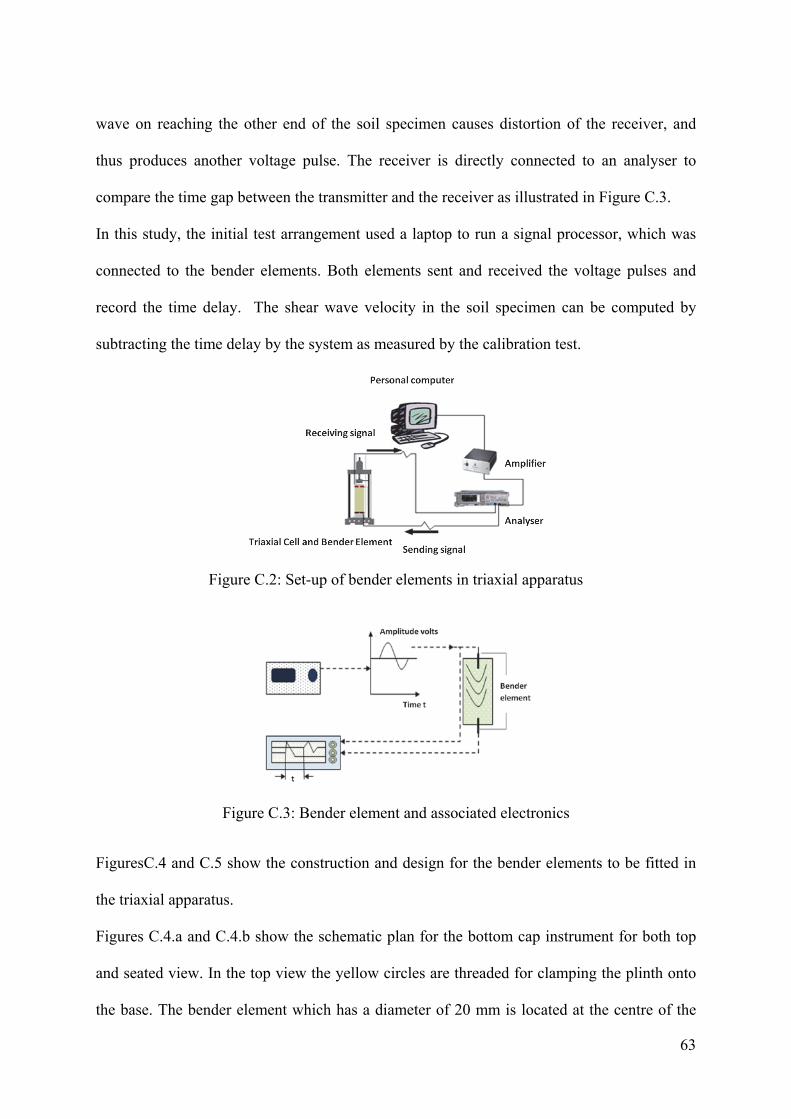
63
wave on reaching the other end of the soil specimen causes distortion of the receiver, and
thus produces another voltage pulse. The receiver is directly connected to an analyser to
compare the time gap between the transmitter and the receiver as illustrated in Figure C.3.
In this study, the initial test arrangement used a laptop to run a signal processor, which was
connected to the bender elements. Both elements sent and received the voltage pulses and
record the time delay. The shear wave velocity in the soil specimen can be computed by
subtracting the time delay by the system as measured by the calibration test.
Figure C.2: Set-up of bender elements in triaxial apparatus
Figure C.3: Bender element and associated electronics
FiguresC.4 and C.5 show the construction and design for the bender elements to be fitted in
the triaxial apparatus.
Figures C.4.a and C.4.b show the schematic plan for the bottom cap instrument for both top
and seated view. In the top view the yellow circles are threaded for clamping the plinth onto
the base. The bender element which has a diameter of 20 mm is located at the centre of the
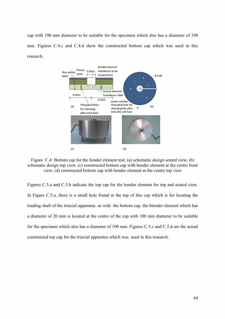
64
cap with 100 mm diameter to be suitable for the specimen which also has a diameter of 100
mm. Figures C.4.c and C.4.d show the constructed bottom cap which was used in this
research.
Figure C.4: Bottom cap for the bender element test; (a) schematic design seated view, (b) schematic design top view, (c) constructed bottom cap with bender element at the centre front
view, (d) constructed bottom cap with bender element at the centre top view
Figures C.5.a and C.5.b indicate the top cap for the bender element for top and seated view.
In Figure C.5.a, there is a small hole found at the top of this cap which is for locating the
loading shaft of the triaxial apparatus. as with the bottom cap, the blender element which has
a diameter of 20 mm is located at the centre of the cap with 100 mm diameter to be suitable
for the specimen which also has a diameter of 100 mm. Figures C.5.c and C.5.d are the actual
constructed top cap for the triaxial apparatus which was used in this research.

65
Figure C.5: Top cap for the bender element test; (a) schematic design seated view, (b) schematic design top view (c) constructed top cap with bender element at the centre front
view, (d) constructed top cap with bender element at the centre top view
The recommended methodology was the routine procedure of a drained consolidation
sequence in a triaxial cell followed by undrained shearing (Head, 1986). The only additional
process is that S-wave velocity measurements are to be taken at each stage of the test using
bender element with top cap and bottom pedestal as shown in Figures C.4 and C.5.
Bender element test was an original intention of this research, but repeated equipment
malfunctions precluded its use and the test programme presented herein was devised to
achieve the project’s objectives.]
Methods of Analysis for Acoustic Properties
The analysis of the test results for the Kaolin Clay sample under isotropic stress conditions
are outlined here. In triaxial test and the relation between them is the Poisson’s ratio in
undrained test conditions. In the analysis of bender element tests the time delay between the
transducer and receiver signals allows the calculation of the shear wave velocity , Vs, and then
the shear modulus, G (Equation 3.8). The equipment for this test was created and the

66
preliminary tests and the geotechnical properties of the Kaolin were carried out and
established respectively, but due to some difficulties with the equipment, the results were not
reliable so an alternative suitable seismic surface wave method has been considered.
Related Documents