Correlation and Dependency in Risk Management - …€¦ · Correlation and Dependency in Risk Management Paul Embrechts, Alexander McNeil & Daniel Strauman Departement Mathematik,

Correlation and Dependency in Risk Management

Paul Embrechts, Alexander McNeil & Daniel Strauman Departement Mathematik, ETH Zentrum, CH 8092 Ziirich

Tel: +41 1 632 61 62, Fax: $41 1 632 15 23 embrechts/mcneil/[email protected]

January 1999

Abstract

Modern risk management calls for an understanding of stochastic dependence going beyond simple linear correlation. This paper deals with the static (non- time-dependent) case and emphasizes the copula representation of dependence for a random vector. Linear correlation is a natural dependence measure for multivariate normally and, more generally, elliptically distributed risks but other dependence concepts like comonotonicity and rank correlation should also be un- derstood by the risk management practitioner. Using counterexamples the falsity of some commonly held views on correlation is demonstrated; in general, these fal- lacies arise from the naive assumption that dependence properties of the elliptical world also hold in the non-elliptical world. In particular, the problem of finding multivariate models which are consistent with prespecified marginal distributions and correlations is addressed. Pitfalls are highlighted and simulation algorithms avoiding these problems are constructed.

Keywords: Risk management; correlation; elliptic distributions; rank corre- lation; dependency; copula; comonotonicity; simulation; Value-at-Risk; coherent risk measures.

1 Introduction

1.1 Correlation in insurance and finance

In financial theory the notion of correlation is central. The Capital Asset Pricing Model (CAPM) and the Arbitrage Pricing Theory (APT) use correlation as a measure of dependence between different financial instruments and employ an elegant theory, which is essentially founded on an assumption of multivariate normally distributed returns, in order to arrive at an optimal portfolio selection. Although insurance has traditionally been built on the assumption of independence and the law of large numbers has governed the determination of premiums, the increasing complexity of insurance and reinsurance products has led recently to increased actuarial interest in the modelling of dependent risks; an example is the emergence of more intricate multi-line products.

-227-

The current quest for a sound methodological basis for integrated risk management also raises the issue of correlation and dependency. Although contemporary financial risk management revolves around the use of correlation to describe dependence between risks, the inclusion of non-linear derivative products invalidates many of the distributional assumptions underlying the use of correlation. In insurance these assumptions are even more problematic because of the typical skewness and heavy-tailedness of insurance claims data.

Recently, within the actuarial world, dynamic financial analysis (DFA) has been heralded as a way forward for integrated risk management of the investment and un- derwriting risks to which an insurer (or bank) is exposed. DFA is essentially a Monte Carlo or simulation-based approach to the joint modelling of risks. This necessitates model assumptions that combine information on marginal distributions together with ideas on interdependencies. The correct implementation of a DFA-based risk manage- ment system certainly requires a proper understanding of the concepts of dependency and correlation.

1.2 Correlation as a source of confusion

Correlation, as well as being a ubiquitous concept in modern insurance and finance, is also frequently a misunderstood concept. Some of the confusion may arise from the literary use of the word to cover any notion of dependency. To a mathematician corre- lation is only one particular measure of stochastic dependency among many. It is the canonical measure in the world of multivariate normal distributions, and more generally for spherical and elliptical distributions. However, empirical research in insurance and finance shows that the distributions of the real world are seldom in this class.

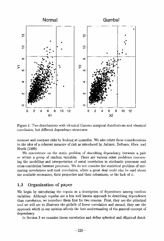
As motivation for the ideas of this paper we include Figure 1 showing 1000 reali- sations from two different bivariate probability models for (X, Y)“. In both models X and Y have identical gamma marginal distributions and an identical linear correlation of 0.7. However, it is clear that the dependence between X and Y in the two models is qualitatively quite different and, if we consider the random variables to represent in- surance losses, the second model is the more dangerous model from the point of view of an insurer, since extreme losses have a tendency to occur together. We return to this example in Example 1; for the time-being we note that the dependence in the two models cannot be distinguished on the grounds of correlation alone.

The main aim of the paper is to collect and clarify the essential ideas of depen- dence, linear correlation and rank correlation that anyone wishing to model dependent phenomena should know. In particular, we highlight a number of important fallacies concerning correlation which arise when we work with models other than the multivari- ate normal. Some of the pitfalls which await the end-user are quite subtle and perhaps counter-intuitive.

We are particularly interested in the problem of constructing multivariate distribu- tions which are consistent with given marginal distributions and correlations, since this is a question that anyone wanting to simulate dependent random vectors, perhaps with a view to DFA, is likely to encounter. We look at the existence and construction of solu- tions and the implementation of algorithms to generate random variates. Several other ideas recur throughout the paper. At several points we look at the effect of dependency structure on the Value-at-Risk or VaR under a particular probability model, i.e. we

-228-

Normal Gumbel

N

0

co

F w

d

N

0

l I l

l ,i::l’

.

0 2 4 6 8 10 12

Xl

cu.

0.

.

.

. . . .

. .*.

.

0 2 4 6 8 10 12

x2

Figure 1: Two distributions with identical Gamma marginal distributions and identical correlation, but different dependence structures

measure and compare risks by looking at quantiles. We also relate these considerations to the idea of a coherent measure of risk as introduced by Artzner, Delbaen, Eber, and Heath (1999).

We concentrate on the static problem of describing dependency between a pair or within a group of random variables. There are various other problems concern- ing the modelling and interpretation of serial correlation in stochastic processes and cross-correlation between processes. We do not consider the statistical problem of esti- mating correlations and rank correlation, where a great deal could also be said about the available estimators, their properties and their robustness, or the lack of it.

1.3 Organization of paper

We begin by introducing the copula as a description of dependence among random variables. Although copulas are a less well known approach to describing dependence than correlation, we introduce them first for two reasons. First, they are the principal tool we will use to illustrate the pitfalls of linear correlation and second, they are the approach which in our opinion affords the best understanding of the general concept of dependency.

In Section 3 we examine linear correlation and define spherical and elliptical distri-

-229-

butions, which constitute, in a sense, the natural environment of the linear correlation. Section 4 is devoted to a discussion of alternative dependence concepts and measures including comonotonicity and rank correlation. Three of the most common fallacies concerning linear correlation and dependence are presented in Section 5. In Section 6 we explain how dependent random vectors may be simulated using correct methods.

Some essential results are stated as propositions and theorems without proofs; a longer version of this paper on our web site (http: //uwu.math.ethz. ch/-mcneil) provides full details (Embrechts, McNeil, and Straumann 1999).

2 Dependence and copulas

2.1 What is a copula?

The dependence between the random variables Xi,. . . , X, is completely described by their joint distribution function

F(Xl,. . . ,xn)=PIX1~xl,... , xl 5 x,1.

The idea of separating F into a part which describes the dependence structure and parts which describe the marginal behaviour only, has led to the concept of a copula.

Suppose we transform the random vector X = (Xi,. . , X,)’ component-wise to have standard uniform (0,l) marginal distributions. For simplicity we assume to begin with that Xi,... , X, have continuous marginal distributions Fi, . . , F,,, so that this can be achieved by component-wise application of the the probability-integral transformation. The joint distribution function C of (Fi(Xi), . . , F,,(X,,))t is then called the copula of the random vector X or the multivariate distribution F. It follows that

Fh, ,xn) = Wi(Xd 5 Flh), . . . , WG) I E&n)1 (1) = Wi(xd, . . , F~(GJ).

Definition 1. A copula is the distribution function of a random vector in R” with standard uniform marginals. Alternatively a copula is any function C : [0, l]” + [0, l] which has the three properties:

1. C(Zi,... , z,) is increasing in each component zi.

2. C(1,. , l,Zi, 1,. . ,l) = 5; for all i E (1,. . . ,n}, z; E [O,l].

3. For all (ai,. , a,,), (bi,. . , b,) E [0, 1)” with ai 5 bi

i:. . . ~(-l)‘l+...+‘~~(zli,, . . . ,2”&) 2 0, i1=1 in=1

where ~jl = aj and xj2 = bj.

These two alternative definitions can be shown to be equivalent. It is easily verified that the first definition in terms of a multivariate distribution function with standard uniform marginals implies the three properties above: property 1 is clear; property 2

-230-

follows from the fact that the marginals are uniform-(0, 1); property 3 is true because the sum can be interpreted as P[ai 5 Xi 2 b,, . . ,a, 2 X, 5 b,], which is non-negative.

For any continuous multivariate distribution the representation (1) holds for a unique copula C. If Fi, . , F,, are not all continuous it can still be shown (Schweizer and Sklar 1983, Chapter 6) that the joint distribution function can always be expressed as in (l), although in this case C is no longer unique and we refer to it as a possible copula of F. The representation (1) suggests that we interpret a copula associated with (Xi,. . Xn)t as being the dependence structzlre. This makes particular sense when all the Fi are continuous and the copula is unique; in the discrete case there will be more than one way of writing the dependence structure.

2.2 Examples of copulas

For independent random variables the copula trivially takes the form

C(Xl,... ,x,)=xl...:xn.

We now consider some particular copulas for pairs of random variables (X, Y)” having continuous distributions. The Gaussian copula is *-yz) s J *-l(Y)

CpNo(x, Y) = 1

-a3 -cm 2741 - py exp 1

-(s2 - @St + 6 dsdt,

‘41 - d) >

(2)

where -1 < p < 1 and @ is the univariate standard normal distribution function. Variables with standard normal marginal distributions and this dependence structure, i.e. variables with distribution function C~(@(Z), a(y)), are standard bivariate normal variables with correlation coefficient p.

Another well-known copula is the Gumbel or logistic copula (Gumbel 1961)

Cp(x,y) = exp [ - { (- logz)“’ + (- logY)li”}~] 9

where 0 < p < 1 is a parameter which controls the amount of dependence between X and Y; p = 1 gives independence. This copula, unlike the Gaussian, is a copula which is consistent with bivariate extreme value theory and could be used to model the limiting dependence structure of component-wise maxima of bivariate random samples (Joe 1997, Galambos 1987).

Many copulas and methods to construct them can be found in the literature; see in particular Hutchinson and Lai (1990) or Joe (1997).

2.3 Invariance

An attractive and important feature of the copula representation of dependence is that the dependence structure as summarized by a copula is invariant under increasing and continuous transformations of the marginals.

Proposition 1. Zf (Xl,. . . , X,,)’ has copda C and Tl, . . , T, are increasing continuous functions, then (Tl(Xl), . , T,(X,))t also has copula C.

-231-

Remark In the case where all marginal distributions are continuous, increasing (but not necessarily continuous) transformations preserve the copula (Schweizer and Sklar 1983).

As a simple illustration of the relevance of this result, suppose we have a probability model (multivariate distribution) for dependent insurance losses of various kinds. If we decide that our interest now lies in modelling the logarithm of these losses, the copula will not change. Similarly if we change from a model of percentage returns on several financial assets to a model of logarithmic returns, the copula will not change, only the marginal distributions.

3 Linear Correlation

3.1 Correlation and its strengths

Definition 2. The linear correlation coefficient between X and Y is

coqx, Y] dXpY) = pjjqqq’

where Cov[X, Y] is the covariance between X and Y, Cov[X, Y] = E[XY) - E[X]E[Y].

The linear correlation is a measure of linear dependence. In the case of independent random variables, p(X,Y) = 0 since Cov[X,Y] = 0. In the case of perfect linear dependence, i.e. Y = aX + b a.s. or P[Y = aX + b] = 1 for a E R \ {0}, b E R, we have p(X, Y) = fl. Correlation fulfills the linearity property

P(QX + P, YY + 6) = sgn(a .7MX, Y),

when a,y E lR \ {0}, @, 6 E R. Correlation is thus invariant under positive affine transformations, i.e. strictly increasing linear transformations.

The generalisation of correlation to more than two random variables is straightfor- ward. For random vectors X = (Xi,. . . ,X,,) and Y = (Yi,. . . ,Y,) in llP we can summarise all pairwise covariances and correlations in n x n matrices Cov[X,Y] and p(X, Y). As long as the corresponding variances are finite we define

Cov[X, Y]ij := Cov[X;, yj],

p(X, Y)ij := p(X;, Yj) 1 2 i, j 5 71.

It is well known that these matrices are symmetric and positive semi-definite. Often one considers only pairwise correlations between components of a single random vector; in this case we set Y = X and consider p(X) := p(X, X) or Cov[X] := Cov[X, X].

The popularity of linear correlation can be explained in several ways. Correlation is often straightforward to calculate. For many bivariate distributions it is a simple matter to calculate second moments (variances and covariances) and hence to derive the correlation coefficient.

Moreover, correlation and covariance are easy to manipulate under linear operations. Under affine linear transformations A : R” -+ EP, z H Ax + a and B : W” -+ W”, x C) Bx + 6 for A, B E WmX”, a, b E IR”’ we have

Cov[AX + a, BY + b] = ACov[X, Y]Bt.

-232-

A special case is the following elegant relationship between variance and covariance for a random vector. For every linear combination of the components otX with cy E R”,

2[dX) = &0v[X]ck.

Thus, the variance of any linear combination is fully determined by the pairwise covari- antes between the components. This fact is commonly exploited in portfolio theory.

A third reason for the popularity of correlation is its naturalness as a measure of dependence in multivariate normal distributions and, more generally, in multivariate spherical and elliptical distributions, as will shortly be discussed. First, we mention a few disadvantages of correlation.

3.2 Shortcomings of correlation

l The variances of X and Y must be finite or the linear correlation is not defined. This is not ideal for a dependency measure and causes problems when we work with heavy-tailed distributions. For example, the covariance and the correlation between the two components of a bivariate t,-distributed random vector are not defined for v 2 2. Non-life actuaries who model losses in different business lines with infinite variance distributions must be aware of this.

. Independence of two random variables implies they are uncorrelated (linear corre- lation equal to zero) but zero correlation does not in general imply independence. A simple example where the covariance disappears despite strong dependence be- tween random variables is obtained by taking X N N(O, l), Y = X2, since the third moment of the standard normal distribution is zero. Only in the case of the rnultivatiate normal is it permissible to interpret uncorrelatedness as imply- ing independence. This implication is no longer valid when only the marginal distributions are normal and the joint distribution is non-normal.

. Linear correlation has the serious deficiency that it is not invariant under non- linear strictly increasing transformations T : R -S R. For two real-valued random variables we have in general

P(TW, W’)) # P(K 0

3.3 Spherical and elliptical distributions

The spherical distributions extend the standard multivariate normal distribution &(O, 1), i.e. the distribution of independent standard normal variables. They provide a family of symmetric distributions for uncorrelated random vectors with mean zero.

Definition 3.

A random vector X = (Xi, . . . , X,,)’ has a spherical distribution if for every orthogonal map U E R”‘” (i.e. maps satisfying UP = VU = Inrn)

ux =,j x.

-233-

The characteristic function $(t) = IE[exp(#X)] of such distributions takes a partic- ularly simple form. There exists a function 4 : lI& --t W such that $(t,) = $(t”t) = b(t;+...+t;). Tl’ f us unction is the characteristic generator of the spherical distribution and we write

If X has a density f(x) = f(~1,. . ,z,) then th’ is is equivalent to f(x) = g(xtx) = g(z: + . . . + $,) for some function g, so that the spherical distributions are best in- terpreted as those distributions whose density is constant on spheres. Some other ex- amples of densities in the spherical class are those of the multivariate t-distribution with v degrees of freedom f(x) = c(1 + x~x/v)-(“+“)‘~ and the logistic distribution j(x) = cexp(-xtx)/[l + exp(-x”x)]“, where c is a generic normalizing constant. Note that these are the distributions of uncorrelated random variables but, contrary to the normal case, not the distributions of independent random variables. In the class of spherical distributions the multivariate normal is the only distribution of independent random variables (Fang, Kotz, and Ng 1987, p. 106).

The spherical distributions admit an alternative stochastic representation. X N &(c$) if and only if

X =d R . U, (4)

where the random vector U is uniformly distributed on the unit hypersphere S,-, = {xlxtx = 1) in R” and R 2 0 is a positive random variable, independent of U (Fang, Kotz, and Ng 1987, p. 30). Spherical distributions can thus be interpreted as mixtures of uniform distributions on spheres of differing radius in R”. For example, in the case of the standard multivariate normal distribution the generating variate R N a, and in the case of the multivariate t-distribution with v degrees of freedom R’/n - F(n, v), where F denotes an F-distribution.

Elliptical distributions extend the multivariate normal N,,(p, C), i.e. the distribution with mean p and covariance matrix C. Mathematically they are the affine maps of spherical distributions in W.

Definition 4. Let T : R” -+ W”, x H Ax + p, A E IP”, ,u E W” be an affine map. X has an elliptical distribution if X = T(Y) and Y N S,,(d).

Since the characteristic function can be written as

$(t) = IE[exp(&(AY + p))] = exp(#p)d(t%),

where C := AAt, we denote the elliptical distributions

For example, nl,(p,C) = E,(p, C,$) with 4(t) = exp(-t’/2). I f Y has a density J(y) = f(yl,. . , y,,) and if A is regular (det(A) # 0 so that C is positive definite), then X = AY + p has density

g(x) = &jr) ----f((x - ,q-‘(x - P)),

-234-

and the contours of equal density are now ellipsoids. Knowledge of the distribution of X does not completely determine the elliptical

representation E,(p, C, 4); it uniquely determines p but C and 4 are only determined up to a positive constant. In particular (if second moments are finite) C can be chosen so that it is directly interpretable as the covariance matrix of X, although this is not always standard. An elliptical distribution is thus fully described by its mean, its covariance matrix and its characteristic generator.

We now consider some of the reasons why correlation and covariance are natural measures of dependence in the world of elliptical distributions. First, many of the prop- erties of the multivariate normal distribution are shared by the elliptical distributions. Linear combinations, marginal distributions and conditional distributions of elliptical random variables are also elliptical and can largely be determined by linear algebra us- ing knowledge of covariance matrix, mean and generator. This is summarized in the following properties.

l Any linear combination of an elliptically distributed random vector is also elliptical with the same characteristic generator 4. If X N E,(h, C,4) and B E IPF”, b E W”. then

BX + b - E,(Bp + b, BCBt, 4).

It is immediately clear that the components Xi,. . . ,X, are all symmetrically distributed random variables of the same type (i.e. having the same distribution up to a change of scale and location

l The marginal distributions of elliptical distributions are also elliptical with the same generator. Let X = (Xi,Xz)t N E,(C,p, 4) with X1 E llP, Xs E lP,

p + q = n. Let E[X] = (~1, ~4, ~1 E RP, ~2 E lP and C = Cl1 Cl2

( > x21 x22 . Then

X1 N Q&l> %I, $1, X2 - Eqb2, C22,4).

l We assume that C is strictly positive definite. The conditional distribution of Xi given X2 is also elliptical, although in general with a different generator $:

Xl/X2 N Epbm &1.2ri% (5)

where pi.2 = ,ui + C&Y~(X2 - pa), Cii.2 = Cii - &&~Csi. The distribution of the generating variable R corresponding to 3 is the conditional distribution

J(X - P)twx - ,4 - (X2 - P2)%2yX2 - P2) 1x2.

In the case of multivariate normality we have R =,, ,@ and &(.) = 4(.), so that the conditional distribution is of the same type as the unconditional; for general elliptical distributions this is not true.

Since the type of all marginal distributions is the same, we see that an elliptical distribution is uniquely determined by its mean, its covariance matrix and knowledge

-23%

of this type. Alternatively the dependence structure (copula) of a continuous elliptical distribution is uniquely determined by the correlation matrix and knowledge of this type. An important question is, which univariate types are possible for the marginal distribution of an elliptical distribution in R” for any n E N? Without loss of generality, it is sufficient to consider the spherical case (Fang, Katz, and Ng 1987, p. 48-51). F is the marginal distribution of a spherical distribution in R” for any n E N if and only if F is a mixture of centred normal distributions. In other words, the density f = F’ is of the form,

where G is a distribution function on [0, co) with G(0) = 0. The corresponding spherical distribution has the alternative stochastic representation

x =,j 69. z, (7)

where S N G, Z N &(O, I,,,,) and S and Z are independent. For example, the multivariate t-distribution with v degrees of freedom can be constructed by taking S N

WI/Z.

3.4 Covariance and elliptical distribution in risk management

A further important feature of the elliptical distributions is that these distributions are amenable to the standard approaches of risk management. They support both the use of Value-at-Risk (VaR) as a measure of risk and the variance-covariance (Markowitz) ap- proach to risk management and portfolio optimization. Suppose that X = (X,, . . . , X,$ represents n risks with an elliptical distribution and that we consider linear portfolios of such risks {Z = CyC1 XiXi ( X; E Iw} with distribution Fz. The use of Value-at-Risk VaR,(Z) = inf{z E Iw : F,(z) > cr} as a measure of the risk of a portfolio Z makes sense because VaR is a coherent risk measure in this world, i.e. it is positive homogeneous, translation-invariant and sub-additive (Artzner, Delbaen, Eber, and Heath 1999).

Moreover, the use of any positive homogeneous, translation-invariant measure of risk to rank risks or to determine optimal risk-minimizing portfolio weights under the condition that a certain return is attained, is equivalent to the Markowitz approach where the variance u”[Z] is used as risk measure. Alternative risk measures such as VaR, or expected shortfall, E[Z 1 Z > VaF&(Z)], g ive i d f f erent numerical values, but have no effect on the management of risk. We make this more precise in the following theorem.

Theorem 1. Suppose X N E,(p, C,4) with D”[Xi] < CO, for all i. Let P = {Z = Cr=, X,X, 1 Xi E R} be the set of all linear portfolios. Then the following are true.

1. (Subadditivity of VaR.) For any two portfolios Z1, Z, E P and 0.5 5 (Y < 1,

VuR,(Z1 + Zz) 5 VaR,(Zl) + VaRb(ZZ).

2. (Equivalence of variance and coherent risk measurement.) Let e be a real-valued risk measure on the space of real-valued random variables which depends only on the

-236-

distribution of a random variable X. Suppose this measure is positive homogeneous and translation-invariant so that it satisfies (1) e(AX) = A@(X), VA 2 0 and (2) e(X+c)= e(X)+c, t/c E R. Then for&,& E P

3. (Markowitz risk-minimizing portfolio.) Let & = {A E lP 1 x7=, A, = l,EIXtX] = T} be the set of portfolio weights giving expected return r. Then

argminx,Ee(X’X) = argminAEea2[AtX].

4 Alternative dependence concepts

4.1 Comonotonicity

For every copula the well-known FrCchet bounds apply (FrBchet 1957),

max{zl + . ~~~42,-1,O}~C(x~ ,..., z,)<min{q ,..., z,}; , \ , (8) Qh,... 4”) C.(Zl,... 3%“)

these follow from the fact that every copula is the distribution function of a random vector (VI,. . , Un)f with Ui - U(O,l). In the case n = 2 the bounds Cr and C, are themselves cop&s since, if U N U(0, l), then

C&l, x2) = B[U<q,l-Lr<Q]

Gblr x2) = W-J 5 21, u 5 %I,

so that Cc and C, are the bivariate distribution functions of the vectors (U, 1 - U)t and (U, U) t respectively.

The distribution of (U, 1 - U)t has all its mass on the diagonal between (0,l) and (l,O), whereas that of (U, V)’ has its mass on the diagonal between (0,O) and (1,l). In these cases we say that Ct and C, describe perfect positive and perfect negative dependence respectively. This is formalized in the following theorem which gives two alternative definitions of comonotonicity

Theorem 2. Let (X, Y)’ have one of the Fre’chet copulas C, OT C,, so that F(xl, x2) = max{F1(zl) +F~(zz) - 1,0} or F(zl, 22) = min{Fl(zl), &(x2)} respectively. Then there exist two monotonic functions u, v : IR -+ W and a real-valued random variable Z so that

(X, v =d (u(Z), v(Z))“,

with u increasing and u decreasing in the former case and with both increasing in the latter. The converse of this result is also true.

Definition 5. If (X, Y)” has copula C, then X and Y are said to be comonotonic; if it has copula Cl they are said to be countermonotonic.

-237-

Remark We have not assumed the continuity of Fi and Fz in this definition. If there are discontinuities then CL and C, are to be interpreted as possible but not unique copulas of (X, Y)“. In the case of continuous marginals (X, Y)” has a unique copula C and the following are equivalent definitions of countermonotonicity and comonotonicity:

C = Cc * Y = T(X) as., T decreasing

C = C, u Y = T(X) a.s., T increasing. (9)

Ideally we would like a scalar-valued measure of dependence (like correlation) to take the values +l and -1 in the cases of comonotonicity and countermonotonicity respectively. In the case of linear correlation this is not necessarily the case and the attainable values of p(X,Y) depend on the choices of Fi and F& as we later explain. We now introduce rank correlation, a correlation defined at copula level which does handle perfect dependence in the way we desire. For more discussion on the desirable properties of dependency measures see Hutchinson and Lai (1990).

4.2 Rank correlation

Definition 6. Let X and Y be random variables with distribution functions Fl and F2 and joint distribution function F. Spearman’s rank correlation is given by

PSK Y) = dFl(X), F,(Y)), (10)

where p is the usual linear correlation. Let (Xi, Yi) and (X2, YJ be two independent pairs of random variables from F, Then Kendall’s rank correlation is given by

,&(X1 Y) = P[(Xl - &p-l - yz) > 01 - iq(Xl - X2)p-l - yz) < 01. (11)

For the remainder of this section we assume that Fl and F2 are continuous distribu- tions, although some of the properties of rank correlation that we derive can be extended to the case of discrete distributions. Spearman’s rank correlation is then seen to be the correlation of the unique copula C of (X, Y)“.

Both ps and p7 can be considered to be measures of the degree of monotonic de- pendence between X and Y, whereas linear correlation measures the degree of linear dependence only. The generalisation of ps and pr to n > 2 dimensions is analogous to that of linear correlation: we write pairwise correlations in an n x n-matrix.

We collect together the important facts about ps and pr in the following theorem.

Theorem 3. Let X and Y be random variables with continuous distributions Fl and Fz, joint distribution F and copula C. The following are true:

1. If X and Y are independent then ps(X, Y) = p7(X, Y) = 0.

2. -1 5 PS(X,Y),P,(X,Y) I +1.

3. PSV, Y) = 12 S; J;{C(z, Y) - q}dn%

4. ,o,(X, Y) = 4 J; J; C(u, v)dC(u, v) - 1.

-238-

5. For T : R + R strictly monotonic,

ps(T(X), Y) = ps(x’ ‘) T increasing,

-ps(X, Y) T decreasing,

and the same invariance property holds for p7.

6. ps(X, Y) = p7(X, Y) = 1 (j C = C, _ Y = T(X) with T increasing.

7. ps(X,Y) = pT(X,Y) = -1 u C = Cr w Y = T(X) with T decreasing.

The main advantages of rank correlation over ordinary correlation are the theoret- ical ones presented in this result. Rank correlation is a correlation defined at copula level which is thus invariant (or only changes sign) under monotonic transformations. Moreover, it assigns the value 1 in the case of perfect positive dependence and the value -1 in the case of perfect negative dependence.

The main disadvantage is that rank correlations do not lend themselves to the same elegant variance-covariance manipulations that linear correlation facilitates. As far as calculation is concerned, there are csses where rank correlations are easier to calculate and cases where linear correlations are easier to calculate. If we are working, for exam- ple, with multivariate normal or t-distributions then calculation of linear correlation is easier, since first and second moments are easily determined. If we are working with a multivariate distribution which possesses a simple closed-form copula, like the Gum- be1 copula in (3), then moments may be difficult to determine and calculation of rank correlation using Theorem 3 may be easier.

5 Fallacies

In this section it suffices to consider bivariate distributions of the random vector (X, Y)“.

Fallacy 1. Marginal distributions and correlation determine the joint distribution.

This is true if we restrict our attention to the multivariate normal distribution or the elliptical distributions. For example, if we know that (X, Y)” has a bivariate normal dis- tribution, then the expectations and variances of X and Y and the correlation p(X, Y) uniquely determine the joint distribution. However, if we only know the marginal dis- tributions of X and Y and the correlation then there are many possible bivariate distri- butions for (X, Y)“. The distribution of (X, Y) t is not uniquely determined by F1, Fz and p(X, Y). We illustrate this with an example.

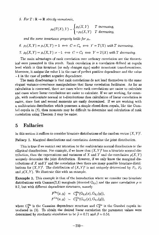
Example 1. This example is that of the Introduction where we consider two bivariate distributions with Gamma(3,l) marginals (denoted Gs,~) and the same correlation p = 0.7, but with different dependence structures, namely

FN%,y) = C,N~(G&),GS,~Y)),

FG”(~,y) = C;“@S,I(~, ‘&J(Y)),

where CT is the Gaussian dependence structure and CF” is the Gumbel copula in- troduced in (3). To obtain the desired linear correlation the parameter values were determined by stochastic simulation to be p” = 0.71 and /? = 0.54.

-239-

We are interested in the behaviour of the joint distribution of (X, Y)’ in the tail. We fix u = VaRo&X) = Va&g(Y) = G$(0.99) an consider the conditional exceedance d probability lF’[Y > u 1 X > u] under the two models. An easy empirical estimation based on Figure 1 yields

fP,h(Y > u 1 x > u] = 3/9,

@,,u[Y > u ) X > u] = 12/16.

In the Gumbel model exceedances of the threshold u in one margin tend to be accom- panied by exceedances in the other, whereas in the Gaussian dependence model joint exceedances in both margins are rare. It appears that there is less diversification of large risks in the Gumbel dependence model and this can be confirmed asymptotically.

For a bivariate distribution with continuous marginals Fl and F2 and copula C it can be verified, under the assumption that the limit exists, that

&n- !P[Y > VaR,(Y) ( X > VaR,(X)] = Jly- P[Y > F;‘(a) ) X > F;‘(Q)]

= lim Co = X E [O 11 a-11- 1 -a

1 I

where ~(CY,CE) = 1 - 2a + C(QI,(Y). I f X = 0 a bivariate model is called asymptoti- cally independent; in the case X > 0 a model is asymptotically dependent. Asymptotic dependence is a property of the copula of the bivariate distribution. It can be shown (see Sibuya (1961) or Resnick (1987, Chapter 5)) that for fi < 1 the Gaussian copula leads to asymptotic independence. For the Gumbel copula C,““(IY,(Y) = a2’ and it is easily shown that X = 2 -2p, so that the model is asymptotically dependent when /3 < 1.

It is clear from these considerations of asymptotic dependence that X + Y produces more very large outcomes under the Gumbel model than under the Gaussian model. For large enough cy we must also have VaRF(X + Y) > VaR,N”(X + Y). Analytic results are more difficult for X + Y but simulations confirm this to be the case. The Value-at- Risk of linear portfolios is not uniquely determined by the marginal distributions and correlation of the constituent risks. See Miiller and Bguerle (1998) for related work on stop-loss risk measures applied to bivariate portfolios under various dependence models

Fallacy 2. Given marginal distributions Fl and F2 for X and Y, all linear correlations between -1 and 1 can be attained through suitable specification of the joint distribution.

This statement is not true. The following theorem shows only certain correlations are possible for given marginal distributions; an example follows the theorem.

Theorem 4. Let (X, Y)” be a random vector with marginals Fl and F2 and unspecified dependence structure; assume 0 < 02[X],u2[Y] < co. Then the set of all possible correlations is a closed interval [pmin,pmu], where Pmin < 0 < pmax. The correlation p = Pmin is attained if and only ij X and Y are countermonotonic. p = pmax is attained if and only if X and Y are comonotonic. Furthermore p,,,i,, = -1 i f f X and -Y are of the same type; pmax = 1 ifl’x and Y are of the same type.

Example 2. Let X N Lognormal(0, 1) and Y N Lognormal(0, a2), o > 0. We wish to calculate Pmin and pmax for these marginals. Note that X and Y are not of the same type

-240-

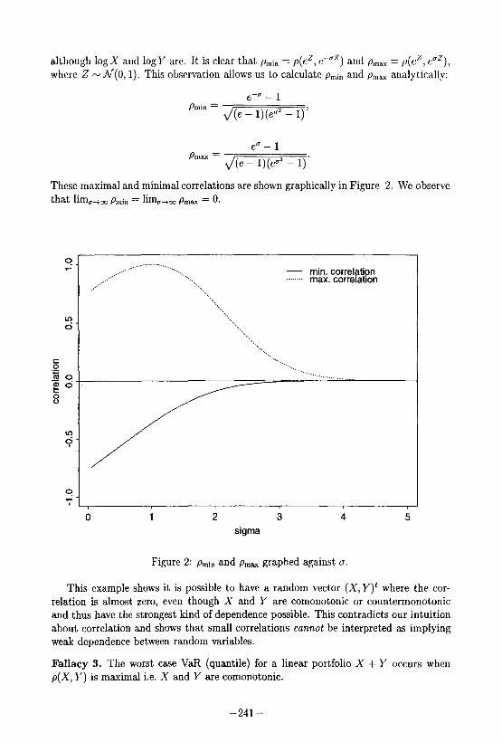
although 1ogX and logy arc. It is clear that prnin = P(eZ, PZ) and pmax = P(eZ, euz), where Z N A/(0,1). This observation allows us to calculate p,,,in and pmax analytically:

Pmin =

e-O - 1

J(e - l)(e”* - 1)’

e” - 1 P

max = J(e - l)(e”’ - 1)‘

These maximal and minimal correlations are shown graphically in Figure 2. We observe that limo.+oo Pmin = limo+, prnax = 0.

,___..-‘- ___.... --.- .__.____

Y._, - min. carrel _.,’

_,_.” ..__ ...._-. max. corre ation B tion

,/ ‘... ‘..,

x, . . . .

‘I..._ ‘...

‘.., ‘...

‘L,_ L_

0 1 2 3 4 5

sigma

Figure 2: Pmin and pmax graphed against u.

This example shows it is possible to have a random vector (X, Y)” where the cor- relation is almost zero, even though X and Y are comonotonic or countermonotonic and thus have the strongest kind of dependence possible. This contradicts our intuition about correlation and shows that small correlations cannot be interpreted as implying weak dependence between random variables.

Fallacy 3. The worst case VaR (quantile) for a linear portfolio X + Y occurs when p(X, Y) is maximal i.e. X and Y are comonotonic.

-241-

It is common to consider variance as a measure of risk in insurance and financial mathematics and, while it is true that the variance of a linear portfolio, a’[X + Y] = cr’[X] + u”[Y] + 2p(X, Y)o[X]o(Y], is maximal when the correlation is maximal, it is in general not correct to conclude that the VaR is also maximal. For elliptical distributions it is true, but generally it is false.

Suppose two random variables X and Y have distribution functions Fi and F, but that their dependence structure (copula) is unspecified. In the following theorem we give an upper bound for VaR,(X + Y).

Theorem 5.

1. For all z E R,

P[X + Y < 4 2 sup c@i(+J’z(~)) = $(z), z+y=z

and there exists a copula C~(“l such that under F(x,y) = Ce(‘)(Fl(x), F2(y) we have lP[X + Y < z] = $(.z), so that the bound is sharp.

2. Let r/~-‘(o) := inf{z ( $(z) > cry), (Y E (0, l), be the generalized inverse ojr,b. Then $‘(a) = inf “+“-1=a{F;1(4 + F,-‘(v)}.

3. The following upper bound for VaR holds:

VaR,(X + Y) 5 I/J-‘((Y).

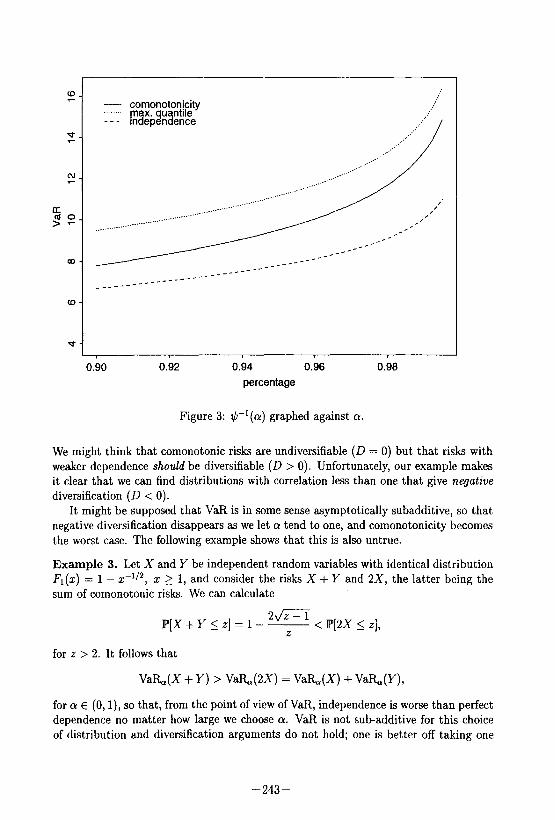
In Figure 3 the upper bound @l(o) is shown for X N Ga,i and Y N Gs,i, for various values of cr.

For comparative purposes VaR,(X + Y) is also shown for the case where X,Y are independent and the case where they are comonotonic. The latter is computed by addition of the univariate quantiles since under comonotonicity VaR,(X + Y) = VaR,(X) + VaR,(Y) (Denneberg 1994). The example shows that for a fixed QI E (0,l) the maximal value of VaR,(X + Y) is considerably larger than the value obtained in the case of comonotonicity. This is not surprising since we know that VaR is not a subadditive risk measure (Artzner, Delbaen, Eber, and Heath 1999) and there are situations where Val&(X + Y) > Va%(X) + VaR,(Y).

In a sense, the difference $-l(o) - (Va%(X) + VaRJY)) quantifies the amount by which VaR jails to be subadditive for particular marginals and a particular cr. For a coherent risk measure e, we must have that Q(X + Y) attains its maximal value in the case of comonotonicity and that this value is Q(X) + Q(Y) (Delbaen 1999). The fact that there are situations which are worse than comonotonicity as far as VaR is concerned, is another way of showing that VaR is not a coherent measure of risk.

For a particular a, the bivariate distribution which yields the largest value of VaR has a correlation (linear or rank) which is strictly less than one. This negates the commonly voiced argument that lower correlation means higher diversification. Suppose we introduce the following measure of diversification:

D = (Va%(X) + Va%(Y)) - VaR,(X + Y).

-242-

cu

a 60 >-

OD

t

- comonotonjcity ._..-.. pax. qu --- lndepen ence %

ntlle

___..____.... -.- ,’ ,’ -- __-- __--

__-- __--

_______------ ____----

__---

___---

0.90 0.92 0.94 0.96 0.98

percentage

Figure 3: $-i(o) graphed against cr.

We might think that comonotonic risks are undiversifiable (D = 0) but that risks with weaker dependence should be diversifiable (D > 0). Unfortunately, our example makes it clear that we can find distributions with correlation less than one that give negative diversification (D < 0).

It might be supposed that VaR is in some sense asymptotically subadditive, so that negative diversification disappears as we let rw tend to one, and comonotonicity becomes the worst case. The following example shows that this is also untrue.

Example 3. Let X and Y be independent random variables with identical distribution Fl(X) = 1 - x-i’s, x > 1, and consider the risks X + Y and 2X, the latter being the sum of comonotonic risks. We can calculate

2&=-l P[X + Y 5 z] = 1 - ___

2 < P[2X 2 z],

for .z > 2. It follows that

Va%(X + Y) > Va%,(2X) = VaR,JX) + Val&(Y),

for o E (0, l), so that, from the point of view of VaR, independence is worse than perfect dependence no matter how large we choose cr. VaR is not sub-additive for this choice of distribution and diversification arguments do not hold; one is better off taking one

-243-

risk and doubling it than taking two independent risks. Diversifiability of two risks is not only dependent on their dependence structure but also on the choice of marginal distribution.

6 Simulation of Random Vectors

There are various situations in practice where we might wish to simulate dependent random vectors (Xi,. . . , X,,)t, perhaps as part of a Monte Carlo or DFA procedure to calculate the risk capital required for dependent risks. It is tempting to approach the problem in the following way:

1. Estimate marginal distributions F,, . . , F,,

2. Estimate matrix of pairwise correlations pij = p(Xi, Xj), i # j

3. Combine this information in some simulation procedure

Unfortunately, the fallacies of the last section show us that the third step represents an attempt to solve an ill-posed problem. There are two main dangers. Given the marginal distributions the correlation matrix is subject to certain restrictions. For example, each pij must lie in an interval [Pmin(Fi, Fj),p,,(F;, Fj)] bounded by the minimal and maximal attainable correlations for marginals Fi and Fj. It is possible that the estimated correlations are not consistent with the estimated marginals so that no corresponding multivariate distribution for the random vector exists. In the case where a multivariate distribution exists it is not unique.

The approach described above is highly questionable, but we will nonetheless show how to construct a multivariate model satisfying the requirements, in the case where such a model exists. We will also consider how simulation can be achieved in the case where Spearman’s rank correlations are given instead of linear correlations; in this case, the correlations being given at copula level, we do not have to worry about compatibility with the marginals, but we still have the problem that solutions are not unique. Finally we will discuss simulation in the most satisfactory case when a particular copula model of the dependency structure is specified along with marginal distributions.

6.1 Given marginals and linear correlations

Suppose we are required to construct a multivariate distribution F in R” which is con- sistent with given marginals distributions Fl, , F,, and a linear correlation matrix p. We assume that p is a proper linear correlation matrix, by which we mean that it is a symmetric, positive semi-definite matrix with -1 2 pij < 1, i, j = 1,. . , n and #Q=l, i=l , . . . , n. Such a matrix will always be the linear correlation matrix of some random vector in R” but we must check it is compatible with the given marginals. Our problem is to find a multivariate distribution F so that if (Xr, . . , X,$ has distribution F the following conditions are satisfied:

XiNFi,i=l,..., n,

p(Xi,Xj)=p*j, i,j=l,..., n. 02)

-244-

In the bivariate case, provided the prespecified correlation is attainable, the construction is simple and relies on the following.

Proposition 2. Let Fl and F2 be two univariate distributions and pmin and prnaw the corresponding minimal and maximal linear correlations. Let p E [pmin, pmax]. Then the biuariate mixture distribution given by

Fhxz) = XFe(xl,~) + (1 - Wu(c,~2), (13)

where X = (prnax - P)/(P,~ - ~~4, FL(zI,Q) = max{Fl(sd + &(xz) - LO} and F,(z~,Q) = min{F~(21), F~(Q)}, has marginals Fl and Fz and linear correlation p.

Remark The mixture distribution is certainly not the unique distribution satisfying our conditions. For p 2 0 the distribution

&1,x2) = ~3’1(~,)~2(~2) + (I- W&1,~2), (14)

with A = (pmax - P)/P~~ also has marginals Fl and F2 and correlation p.

Simulation from the mixture distribution in the theorem is achieved with the following algorithm:

1. Simulate VI, U2 independently from standard uniform distribution.

2. I f U, 5 X take (Xl,X# = (F;1(U2), F;‘(l - Uz))“.

3. I f V~ > X take (X1,X# = (F;l(&), F;‘(U2))t.

Constructing a multivariate distribution in the case n 2 3 is more difficult. For the existence of a solution it is certainly necessary that pmin(Fi, Fj) 5 pij 5 pmu(Fi, Fj), i # j, so that the pairwise constraints are satisfied. In the bivariate case this is sufficient for the existence of a solution to the problem (12) but in the general case it is not sufficient as the following example shows.

Example 4. Let 4, F2 and F3 be Lognormal(0, 1) distributions. Suppose that p is such that p;j is equal to the minimum attainable correlation for a pair of Lognormal(0, 1) ran- dom variables ( M -0.368) if i # j and plj = 1 if i = j. This is both a proper correlation matrix and a correlation matrix satisfying the pairwise constraints for lognormal ran- dom variables. However, since ~12, ~13 and p23 are all minimum attainable correlations, Theorem 4 implies that X1, X2 and X3 are pairwise countermonotonic random variables. Such a situation is unfortunately impossible as is clear from the following proposition.

Proposition 3. Let X, Y and Z be random variables with joint distribulion F and continuous marginals F,, F2 and F3.

1. If (X, Y) and (Y, 2) are pairwise comonotonic then (X, Z) is also comonotonic and F(x, Y, 2) = min{Fl(x), WY), S(z)).

2. If (X, Y) is comonotonic and (Y, Z) as counter-monotonic then (X, Z) is counter- monotonic and F(z, y, z) = max{O, min{F1(z), F2(y)} + F3(2) - 1).

-245-

3. If (X, Y) and (Y, 2) are pairwise countermonotonic then (X, 2) is comonotonic and F(z, y, z) = max{O, min{Fi(z), Fa(z)} + Fs(y) - 1).

The lemma permits us now to state a result concerning existence and uniqueness of solutions to our problem (12) in the special case where random variables are either pairwise comonotonic or countermonotonic.

Theorem 6. Let FI, . . . , F,, n 1 3, be continuous distributions and let p be a (proper) correlation matrix satisfying the following conditions for all i # j, i # k and j # k:

l Pij E {Pmin(Fir Fj), Pm.xx(Fi, Fj)};

l I f Pij = Pmax(Et Fj) and pik = pmax(Fi, Fk) then pjk = pma(Fj, Fk);

l I f Pij = Pmax(Fi, F’) and pik = pmin(Fir Fk) then pjrc = pmin(Fjr Fk);

l IfPij = pmin(KtFj) and ~ik = Pmin(Fir Fk) then pjc = p,,(Fj, Fk).

Then there exists a unique distribution with marginals F,, . . , F,, and correlation matrix p. This distribution is known as an extremal distribution (Tiit 1996). In R” there are 2*-l possible extremal distributions.

Suppose, for example, that p is such that, for some 2 2 m < n, pij is maximal for 1~i,j~morm<i,j~nandminimalforI~i~m<j~nor1~j~m~i~n. In this case simulation from the unique extremal distribution is achieved by taking

(F;‘(U), F;‘(U), , F,-‘(U), F,-:,(I - U), . , F;‘(l - U))“,

where U is standard uniform. For margmals Fi, . . . ,F,,letGj,j=l,... , 2n-1, be the extremal distributions and

let pj, j = 1, . . ,2”-l, be their correlation matrices. Convex combinations

G = ‘2 XjG,, Xj 2 0, ‘5 Xj = 1, j=l j=l

also have the same marginals and a correlation matrix given by p = ci,’ Xjpj. I f we can decompose an arbitrary correlation matrix p in this way, then we can use a convex combination of extremal distributions to construct a distribution which solves the general problem (12); see Tiit (1996) for more details.

A disadvantage of the extremal distributions is that they have no density, since they place all their mass on edges in W”. However, one can think of practical examples where such distributions might still be relevant.

Example 5. Consider two portfolios of credit risks. In the first portfolio we have risks from country A, in the second risks from country B. Portfolio A has a profit-loss distribu- tion FI and portfolio B a profit-loss distribution F2. With probability p the results move in the same direction (comonotonicity); with probability (1 - p) they move in opposite directions (countermonotonicity). This situation can be modelled with the distribution

F(n, ~2) = P. min{Fl(xd,F2(x2)) + Cl- P) m={Fl’l(sd + W34 - ho).

-246-

6.2 Given marginals and Spearman’s rank correlations

This problem has been considered by Iman and Conover (1982) and their algorithm forms the basis of the @RISK computer program.

It is clear that a Spearman’s rank correlation matrix is also a proper linear corre- lation matrix (Spearman’s rank being defined as the linear correlation of ranks). It is not known to us whether a linear correlation matrix is necessarily a Spearman’s rank correlation matrix. That is, given an arbitrary symmetric, positive semi-definite matrix with unit elements on the diagonal and off-diagonal elements in the interval [-1, 11, can we necessarily find a random vector for which this is the rank correlation matrix, or alternatively a multivariate distribution for which this is the linear correlation matrix of the copula? If we estimate a rank correlation matrix from data, is it guaranteed that the estimate is itself a rank correlation matrix? A necessary condition is certainly that the estimate is a linear correlation matrix, but we do not know if this is sufficient.

I f the given matrix is a true rank correlation matrix, then the problem of the ex- istence of a multivariate distribution with prescribed marginals is solved. The choice of marginals is in fact irrelevant and imposes no extra consistency conditions on the matrix.

Iman and Conover (1982) do not attempt to find a multivariate distribution which has exactly the given rank correlation matrix p. They simulate a standard multivariate normal variate (Xi,. ,X,,)’ with linear correlation matrix p and then transform the marginals to obtain (Yi,. . . , Y,)’ = (Fr-‘(@(Xi)), . . . , F;‘(@(X,)))t. The rank correla- tion matrix of Y is identical to that of X. Now

ps(K, Yj) = ps(Xi,Xj) = i arcsin w z PC-&Y Xj) v

and, in view of the bounds (Joag-dev 1984),

5 arcsin f - p 5 0.0181, 1: x

the rank correlation matrix of Y is very close to that which we desire. In the case when the given matrix belongs to an extremal distribution (i.e. comprises only elements 1 and -1) then the error disappears entirely and we have constructed the unique solution.

This suggests a sufficient condition for p to be a Spearman’s rank correlation matrix and how, when this condition holds, we can construct a distribution which has the required marginals and exactly this rank correlation matrix. We define the matrix p by

(15)

and check whether this is a proper linear correlation matrix. I f so, then (Yr, . . , Y,)’ =

(K'(@(Xi)),... , F;‘(O(X,)))” has rank correlation matrix p, where (Xr, . ,X,,)’ is a standard multivariate normal variate with linear correlation matrix F.

In summary, a necessary condition for p to be a rank correlation matrix is that it is a linear correlation matrix and a sufficient condition is that p given by (15) is a linear correlation matrix. We are not aware at present of a necessary and sufficient condition.

A further problem with the approach described above is that we only ever construct distributions which have the copula of the multivariate normal distribution. This depen- dency structure is limited and does not permit asymptotic dependency between random variables, as we have seen.

-247-

6.3 Given marginals and copula

In the case where marginal distributions Fr, . . . , F,, and a copula C(ur, . . . , u,,) are spec- ified a unique multivariate distribution F(zl, . . . , z,) = C(Fl(z), . . . , Fn(z)) satisfying these specifications can be found. The problem of simulating from this distribution is no longer the theoretical one of whether a solution exists, hut rather the technical one of how to perform the simulation. We assume the copula is given in the form of a para- metric function which the modeller has chosen; we do not consider the problem of how copulas might be estimated from data, which is certainly more difficult than estimating linear or rank correlations.

Once we have simulated a random vector @Jr,. . , U,# from C, then the random vector (Flm'(U~), , F;'(U,,))' has distribution F. We assume that calculating the inverses of the marginal distributions presents no problem, although root finding routines may be required. The major technical difficulty lies in simulating realisations from the copula.

Where possible a transformation method can be applied; that is, we make use of multivariate distributions with the required copula for which a multivariate simulation method is already known. For example, to simulate from the bivariate Gaussian cop- ula it is trivial to simulate (.Zr,Z# from the standard bivariate normal distribution with correlation p and then to transform the marginals with the univariate distribution function so that ((a(&), a(&))” is distributed according to the desired copula. For the bivariate Gumbel copula a similar approach can be taken.

Example 6. Consider the Weibull distribution with survivor function q(z) = 1 - F,(s) = exp (-z”) for o > 0, zr 2 0. If we apply the Gumbel copula to this survivor function (not to the distribution function) we get a bivariate distribution with Weibull marginals and survivor function

F(q,z2) = B[Zl > zl,Z2 > z2] = C(F;,(zl),Fl(z2)) = exp[-(zl +z~)~].

Lee (1979) describes a method for simulating from this distribution. We take (Zr, Zz)” = (US’/“, (1 - U)S1/=)t h w ere U is standard uniform and S is a mixture of Gamma distributions with density h(s) = (1-o+os) exp(-s) for s > 0. Then (F1(Zl),Fl(Zz))” will have the Gumbel copula distribution.

Where the transformation method cannot easily be applied, another possible method involves recursive simulation using univariate conditional distributions. We consider the general case n > 2 and introduce the notation

c,(q)..., u;)=C(q ,..., Ui,l)...) l), i=2 ,..., n-l

to represent i-dimensional marginal distributions of C(ur, . . , u,). We write C1(ul) = ‘1~1 and C”(U~,. . , Us) = C(vr,. . ,u,). Suppose that (VI,. . ,U,,)t N C. The condi- tional distribution of Vi given the values of the first i - 1 components of (U,, . , U,# can be written in terms of derivatives and densities of the i-dimensional marginals

Ci(% I ulr.. . , W-1) = ~[UiIUiIU~=Ul,...,Ui-l=~i-l]

-248-

provided both numerator and denominator exist. This suggests that if we can calculate these conditional distributions we can use the algorithm:

0 Simulate a value ui from U(0, 1).

l Fori=2,.. . ,n, simulate a value 21; from Ci(U, ) q, . . , u,-1).

To simulate a value from Ci(u, ( ul,. . ,ui-i) we would in general simulate u from U(0, 1) and then calculate C,:l(u ( ‘1~1,. , ZL,-~), if necessary by numerical root finding.

7 Conclusion

In this paper we have shown some of the problems that can arise when the concept of linear correlation is used with non-elliptical multivariate distributions. In the world of el- liptical distributions correlation is a natural and elegant summary of dependence, which lends itself to algebraic manipulation and the standard approaches of risk management dating back to Markowitz. In the non-elliptical world our intuition about correlation breaks down and leads to a number of fallacies. The first aim of this paper has been to suggest that practitioners of risk management must be aware of these pitfalls and must appreciate that a deeper understanding of dependency is needed to model the risks of the real world.

The second main aim of this paper has been to address the problem of simulating dependent data with given marginal distributions. This question arises naturally when one contemplates a Monte Carlo approach to determining the risk capital required to cover dependent risks. We have shown that the ideal situation is when the multivari- ate dependency structure (in the form of a copula) is fully specified by the modeller. Failing this, it is preferable to be given a matrix of rank correlations than a matrix of linear correlation, since rank correlations are defined at a copula level, and we need not worry about their consistency with the chosen marginals. Both correlations are, however, scalar-valued dependence measures and if there is a multivariate distribution which solves the simulation problem, it will not be the unique solution. The example of the Introduction showed that two distributions with the same correlation can have qualitatively very different dependency structures and, ideally, we should consider the whole dependence structure which seems appropriate for the risks we wish to model.

Acknowledgements

The second author is Swiss Re Research Fellow at ETH Zurich and gratefully acknowl- edges the financial support of Swiss Re. The work of the third author was supported by RiskLab at ETH Zurich.

References

ARTZNER, P., F. DELBAEN, J.-M. EBER, and D. HEATH (1999): ‘Coherent measures of risk,” To appear in Mathematical Finance.

DELBAEN, F. (1999): “Coherent risk measures on general probability spaces,” Preprint ETH Zurich.

-249-

DENNEBERG, D. (1994): Non-additive Measure and Integral. Kluwer Academic Pub lishers, Dordrecht.

EMBRECHTS, P., A. MCNEIL, and D. STRAUMANN (1999): “Correlation and Depen- dency in Risk Management: Properties and Pitfalls,” Preprint ETH Zurich.

FANG, K.-T., S. KOTZ, and K.-W. NG (1987): Symmetric Multivariate and Related Distributions. Chapman & Hall, London.

FRJ?CHET, M. (1957): “Les tableaux de correlation dont les marges sont don&es,” Annales de l’llniversite’ de Lyon, Sciences Mathe’matiques et Astronomie, S&e A, 4, 13-31.

GALAMBOS, J. (1987): The Asymptotic Theory of Eztreme Order Statistics. Kreiger Publishing Co., Melbourne, FL.

GUMBEL, E. J. (1961): “Bivariate logistic distributions,” JASA, 56, 335-349.

HUTCHINSON, T. P., and C. D. LAI (1990): Continuous &variate Distributions, Emphasizing Applications. Rumsby Scientific Publishing, Adelaide.

IMAN, R. L., and W. CONOVER (1982): “A distribution-free approach to inducing rank correlation among input variables,” Communications in Statistics - Simulation and Computation, 11, 311-334.

JOAG-DEV, K. (1984): “Measures of Dependence,” in Handbook of Statistics, ed. by P. R. Krishnaiah, vol. 4, pp. 79-88. North-Holland/Elsevier, New York.

JOE, H. (1997): Multivariate Models and Dependence Concepts. Chapman & Hall, Lon- don.

LEE, L. (1979): “Multivariate distributions having Weibull properties,” Jounzal of Multivariate Analysis, 9, 267-277.

MULLER, A., and N. B~UERLE (1998): “Modelling and comparing dependencies in multivariate risk portfolios,” ASTIN, 28, 59-76.

RESNICK, S. I. (1987): Extreme Values, Regular Variation and Point Processes. Springer, New York.

SCHWEIZER, B., and A. SKLAR (1983): Probabilistic Metric Spaces. North- Holland/Elsevier, New York.

SIBUYA, M. (1961): “Bivariate extreme statistics,” Annals of Mathematical Statistics, 11, 195-210.

TIIT, E. (1996): “Mixtures of multivariate quasi-extremal distributions having given marginals,” in Distributions with Fixed Marginals and Related Topics, ed. by L. Riischendorff, B. Schweizer, and M. D. Taylor, pp. 337-357, Hayward, CA. In- stitute of Mathematical Statistics.

-250-