Correlated Optical and X-ray Variability in LMC X-2

arX

iv:a

stro

-ph/

0307

373v

1 2

1 Ju

l 200

3Mon. Not. R. Astron. Soc. 000, 1–11 (2003) Printed 16 January 2014 (MN LATEX style file v1.4)

Correlated Optical and X-ray Variability in LMC X–2

K.E. McGowan1,2⋆, P.A. Charles2,3, D. O’Donoghue4, A.P. Smale5

1Los Alamos National Laboratory, MS D436, Los Alamos, NM 87545, USA2Department of Physics, University of Oxford, Oxford OX1 3RH3Department of Physics & Astronomy, University of Southampton, Southampton S017 1BJ4South African Astronomical Observatory, PO Box 9, Observatory 7935, Cape Town, South Africa5Laboratory for High Energy Astrophysics, Code 662, NASA/Goddard Space Flight Center, Greenbelt, MD 20771, USA

16 January 2014

ABSTRACT

We have obtained high time resolution (seconds) photometry of LMC X–2 in December1997, simultaneously with the Rossi X-ray Timing Explorer (RXTE), in order to searchfor correlated X-ray and optical variability on timescales from seconds to hours. Wefind that the optical and X-ray data are correlated only when the source is in a high,active X-ray state. Our analysis shows evidence for the X-ray emission leading theoptical with a mean delay of < 20 s. The timescale for the lag can be reconciled withdisc reprocessing, driven by the higher energy X-rays, only by considering the lowerlimit for the delay. The results are compared with a similar analysis of archival dataof Sco X–1.

Key words: binaries: close - stars: individual: LMC X–2, Sco X–1 - X-rays: stars

1 INTRODUCTION

LMC X–2 is the most X-ray luminous low mass X-ray bi-nary (LMXB) known. It was first observed in early satelliteflights (Leong et al. 1971) and observations showed it tovary from LX ∼ 0.6–3 × 1038 erg s−1(Markert & Clark 1975;Johnston, Bradt & Doxsey 1979; Long, Helfand & Grabelsky1981). Using a precise X-ray location Johnston et al. (1979)LMC X–2 was optically identified as a faint, V ∼ 18.8, bluestar (Pakull 1978; Pakull & Swings 1979).

X-ray light curves from EXOSAT (Bonnet-Bidaud etal. 1989) showed that the source was most variable in thehighest energy range (3.6–11 keV), the variability decreasedwith energy and it was almost constant in the lowest en-ergy range (0.9–2.4 keV). LMC X–2 displayed flaring activ-ity which was characterized by a spectral hardening abovean energy of ∼3.6 keV.

The optical spectrum is that of a typical LMXB withweak Hα, Hβ and HeII λ4686 emission superimposed on ablue continuum. The characteristics of the optical spectrum,the relatively soft X-ray spectrum, and the high X-ray tooptical luminosity (LX/Lopt ∼ 600), imply LMC X–2 is sim-ilar to galactic LMXBs (e.g. van Paradijs 1983). The opticalspectrum lacks the Bowen blend, but this is probably due tothe lower metal abundances in the LMC (Johnston, Bradt& Doxsey 1979), which is also used to account for the excep-tionally high X-ray luminosities of the LMC X-ray binaries

⋆ email: [email protected]

(Motch & Pakull 1989). LMC X–2’s similarity to LMXBsin the Galaxy suggested a likely short orbital period (i.e.<∼ 1 d).

However, in spite of a number of studies, the periodof LMC X–2 remains uncertain. Motch et al. (1985) andBonnet-Bidaud et al. (1989) found evidence for a period of∼ 6.4 h, whereas Callanan et al. (1990) found a periodic-ity of 8.15 h, and Crampton et al. (1990) suggested a muchlonger period of ∼ 12.5 days. The only previous simultane-ous optical and X-ray coverage of LMC X–2 was very short(6 h) and showed no correlation between the two light curves(Bonnet-Bidaud et al. 1989). Here we present the results ofmuch more extensive simultaneous optical and X-ray pho-tometry of LMC X–2 from December 1997, the aim of whichwas to search for correlated X-ray and optical variability ontimescales from seconds to hours and to investigate the pre-viously claimed periodicities.

2 OBSERVATIONS AND DATA ANALYSIS

Observations of the optical counterpart of LMC X–2were performed using the UCT–CCD fast photometer(O’Donoghue 1995) at the Cassegrain focus of the 1.9 mtelescope at SAAO, Sutherland on 1997 December 4–6. TheUCT–CCD fast photometer is a Wright Camera 576 × 420coated GEC CCD, which was used half-masked so as to op-erate in frame-transfer mode. In this configuration, only halfof the chip is exposed, and at the end of the integration the

c© 2003 RAS

http://arxiv.org/abs/astro-ph/0307373v1

2 K.E. McGowan et al.

Table 1. Log of high-speed photometry observations of LMC X–2: SAAO 1.9 m.

Start Time Duration Exposure TimeJD +2450000 (hr) (s)

787.306 0.70 2787.355 1.35 2787.425 0.87 5787.510 0.95 2787.558 0.58 2788.306 0.23 2788.423 1.35 10788.490 0.57 10789.286 0.45 2789.315 0.57 2789.422 1.42 2789.489 0.53 2789.558 0.27 2

signal is read out through the masked half. In this way, it ispossible to obtain consecutive exposures of as short as 1 swith no deadtime. White light high-speed photometry runswere carried out with integration times of 2–10 s (see Table1).

As the seeing fluctuated during the observations, pointspread function (PSF) fitting was essential to obtain goodphotometry. The reductions were performed with the iraf

implementation of daophot ii (Stetson 1987). For our pur-poses only the relative brightness of a star is of importance,and so differential photometry was applied to help reducethe effects of any variations in transparency, employing 2bright local standards within our field of view. This resultedin a relative precision of ±0.04 mag per frame.

The X-ray data were obtained using the proportionalcounter array (PCA) instrument on the RXTE satellite be-tween 1997 December 2 18:52 UT and December 7 1:40UT, in an observing strategy designed to achieve the max-imum amount of simultaneous coverage with the opti-cal photometry. Data from all proportional counter unit(PCU) layers and detectors were included in the creationof X-ray light curves in the 2–10 keV energy range. Wechose a time resolution of 1 s, rather than the standard16 s, for cross-correlation purposes. Background subtractionwas performed utilising standard models generated by theRXTE/PCA team. Further information about the X-ray ob-servations can be found in Smale & Kuulkers (2000).

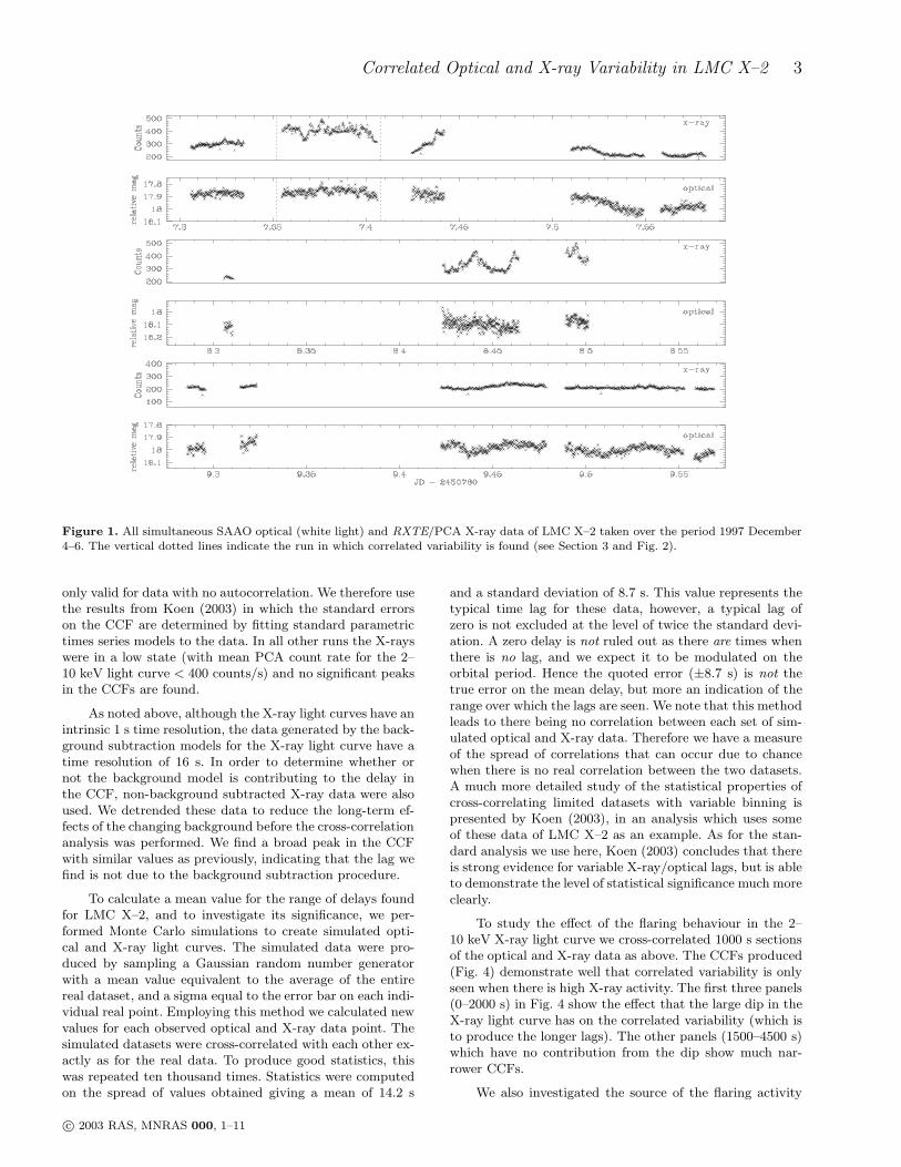
Optical data simultaneous with the RXTE data wereobtained covering 6.6 h, 4.68 h, and 6.8 h respectively on thethree optical observing nights (see Fig. 1). The timing of theX-ray data was measured in Julian Date (Terrestrial Time)[JD(TT)]. The optical timing was measured in JD(UT) andhad to be corrected for the accumulated leap seconds to

produce timings in JD(TT) (see XTE Time Tutorial†).Although the UCT–CCD running in frame transfer

mode can take exposures as fast as 1 s, we found that thecomputer used to store the images had a limit on how fast itcould transfer the data. Hence, the effective exposure timefor the shortest observations is 2.019 s.

† http://legacy.gsfc.nasa.gov/docs/xte/abc/time tutorial.html

The X-ray data has a time resolution of 1 s, the opticaldata 2–10 s. Visual examination of the light curves showsthat the variability in both is on timescales of greater thanmany tens of seconds. Hence we found this variability to bedisplayed most clearly when both X-ray and optical datawere binned into 16 s intervals (Fig. 2). However, to quanti-tatively study the correlation between the two, and to searchfor any delays between the two wavebands, we binned theX-ray light curve onto the corresponding optical light curvetime bins i.e. 2, 5 or 10 s (see Table 1).

3 LMC X–2 TEMPORAL ANALYSIS

LMC X–2 exhibits clear night-to-night variations of severaltenths of a magnitude, fine structure within each night isalso evident (Fig. 1). The intervals of optical photometryare too short to allow detection of the previously quotedorbital periods of 8.15 h and 12.5 d. Furthermore, a periodsearch on the dataset failed to reveal any consistent shorterterm periodicities in the data.

In order to investigate the correlation between theoptical and X-ray data, to determine whether a delay ispresent and to quantify this delay we performed (i) a cross-correlation analysis, and (ii) modelling of the optical lightcurve by convolving the X-ray light curve with a Gaussiantransfer function.

3.1 Cross-correlation

We performed the cross-correlations of each run of opticaland X-ray data by employing a modified version of the In-terpolation Correlation Function, ICF (Gaskell & Peterson1987; Hynes et al. 1998). As our optical and X-ray dataare binned onto the same time resolution, and we edited thelengths of the two time series to be the same, interpolation isnot required. The cross-correlation technique that results iseffectively a Discrete Correlation Function, DCF, similar tothat of Edelson & Krolik (1988). We also implemented codebased on standard cross-correlation function (CCF) routineswhich are again similar to a DCF; both the ICF and CCFmethods agree well.

Concerns have been raised in the literature (see Koen1994) about the validity of cross-correlation as a means tofinding lags within wavebands for a source due to the effectsof the auto-correlation function in the individual time-serieson the CCFs produced. This can lead to the peak in theCCF being shifted from its true value.

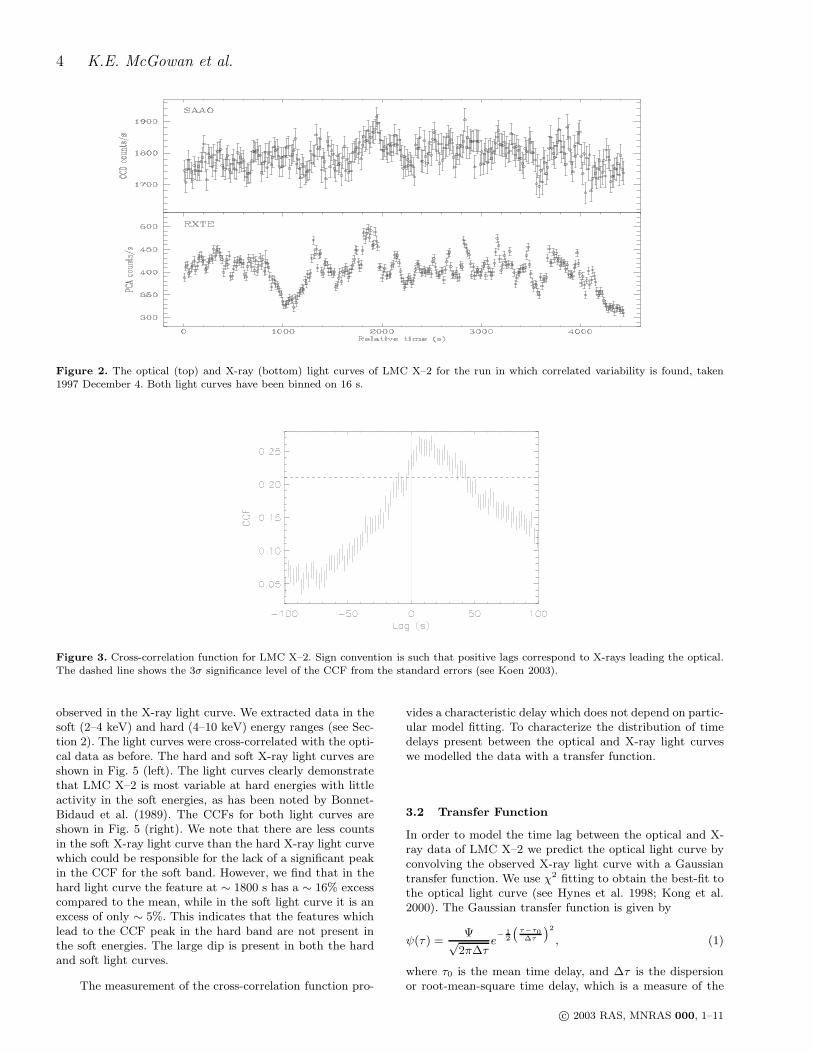
For the one simultaneous run (JD 2450787.355 –2450787.406) where LMC X–2 is seen to be in a bright, ac-tive X-ray state (i.e. flares are present and the mean PCAcount rate in the 2–10 keV light curve is 400 counts/s) abroad peaked CCF is produced. For this run the resultingtime bins are of 2.019 s. The position of the CCF peak in-dicates there is a non-zero delay of order ∼ 20 s betweenthe two datasets. The sign convention of the CCF impliesthat the optical lags the X-rays (Fig. 3). This is expected ifthe delay is attributed to the X-rays heating some part ofthe binary system which in turn produces optical emission.The standard deviation for the CCF for uncorrelated datais given by σn = 1/(n − 2)1/2, where n is the number ofobserved points (Gaskell & Peterson 1987). However, this is

c© 2003 RAS, MNRAS 000, 1–11

Correlated Optical and X-ray Variability in LMC X–2 3

Figure 1. All simultaneous SAAO optical (white light) and RXTE/PCA X-ray data of LMC X–2 taken over the period 1997 December4–6. The vertical dotted lines indicate the run in which correlated variability is found (see Section 3 and Fig. 2).

only valid for data with no autocorrelation. We therefore usethe results from Koen (2003) in which the standard errorson the CCF are determined by fitting standard parametrictimes series models to the data. In all other runs the X-rayswere in a low state (with mean PCA count rate for the 2–10 keV light curve < 400 counts/s) and no significant peaksin the CCFs are found.

As noted above, although the X-ray light curves have anintrinsic 1 s time resolution, the data generated by the back-ground subtraction models for the X-ray light curve have atime resolution of 16 s. In order to determine whether ornot the background model is contributing to the delay inthe CCF, non-background subtracted X-ray data were alsoused. We detrended these data to reduce the long-term ef-fects of the changing background before the cross-correlationanalysis was performed. We find a broad peak in the CCFwith similar values as previously, indicating that the lag wefind is not due to the background subtraction procedure.

To calculate a mean value for the range of delays foundfor LMC X–2, and to investigate its significance, we per-formed Monte Carlo simulations to create simulated opti-cal and X-ray light curves. The simulated data were pro-duced by sampling a Gaussian random number generatorwith a mean value equivalent to the average of the entirereal dataset, and a sigma equal to the error bar on each indi-vidual real point. Employing this method we calculated newvalues for each observed optical and X-ray data point. Thesimulated datasets were cross-correlated with each other ex-actly as for the real data. To produce good statistics, thiswas repeated ten thousand times. Statistics were computedon the spread of values obtained giving a mean of 14.2 s

and a standard deviation of 8.7 s. This value represents thetypical time lag for these data, however, a typical lag ofzero is not excluded at the level of twice the standard devi-ation. A zero delay is not ruled out as there are times whenthere is no lag, and we expect it to be modulated on theorbital period. Hence the quoted error (±8.7 s) is not thetrue error on the mean delay, but more an indication of therange over which the lags are seen. We note that this methodleads to there being no correlation between each set of sim-ulated optical and X-ray data. Therefore we have a measureof the spread of correlations that can occur due to chancewhen there is no real correlation between the two datasets.A much more detailed study of the statistical properties ofcross-correlating limited datasets with variable binning ispresented by Koen (2003), in an analysis which uses someof these data of LMC X–2 as an example. As for the stan-dard analysis we use here, Koen (2003) concludes that thereis strong evidence for variable X-ray/optical lags, but is ableto demonstrate the level of statistical significance much moreclearly.

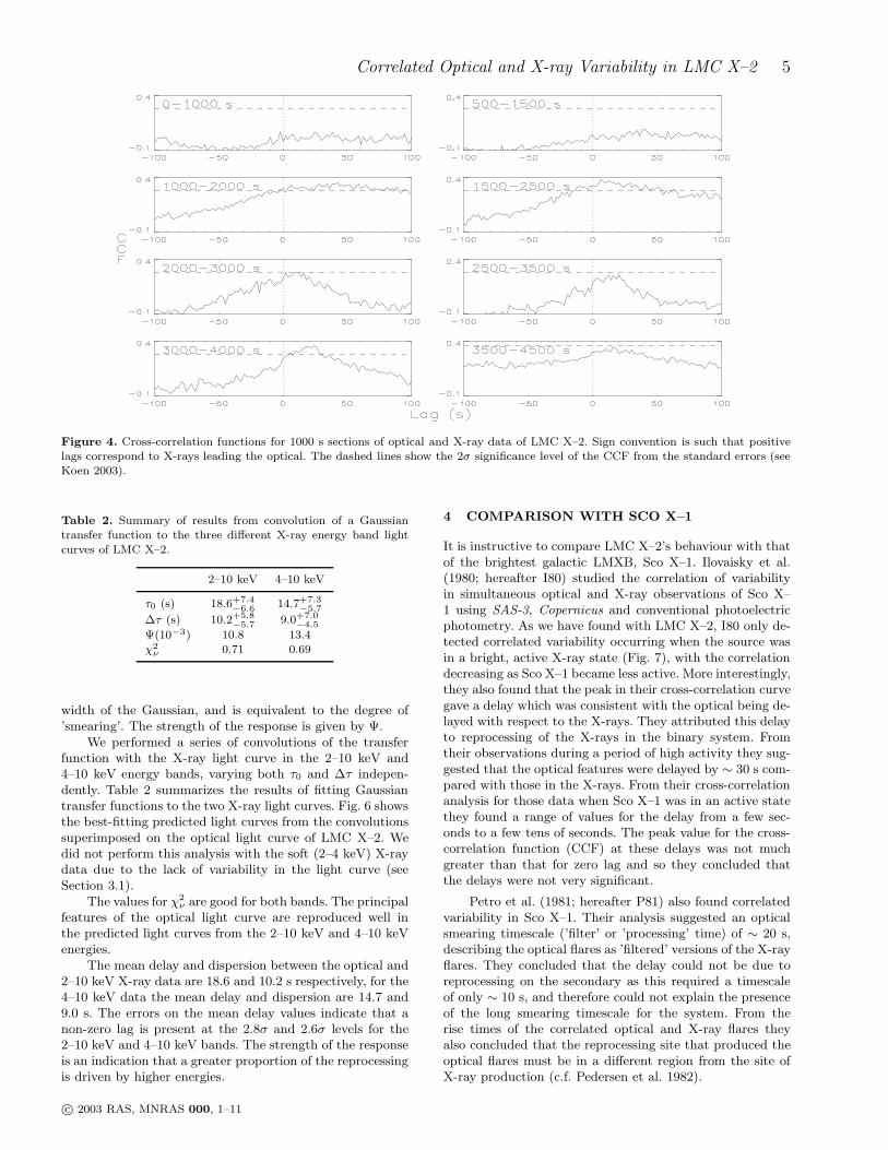
To study the effect of the flaring behaviour in the 2–10 keV X-ray light curve we cross-correlated 1000 s sectionsof the optical and X-ray data as above. The CCFs produced(Fig. 4) demonstrate well that correlated variability is onlyseen when there is high X-ray activity. The first three panels(0–2000 s) in Fig. 4 show the effect that the large dip in theX-ray light curve has on the correlated variability (which isto produce the longer lags). The other panels (1500–4500 s)which have no contribution from the dip show much nar-rower CCFs.

We also investigated the source of the flaring activity

c© 2003 RAS, MNRAS 000, 1–11


Figure 2. The optical (top) and X-ray (bottom) light curves of LMC X–2 for the run in which correlated variability is found, taken1997 December 4. Both light curves have been binned on 16 s.

Figure 3. Cross-correlation function for LMC X–2. Sign convention is such that positive lags correspond to X-rays leading the optical.The dashed line shows the 3σ significance level of the CCF from the standard errors (see Koen 2003).

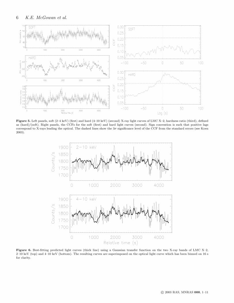
observed in the X-ray light curve. We extracted data in thesoft (2–4 keV) and hard (4–10 keV) energy ranges (see Sec-tion 2). The light curves were cross-correlated with the opti-cal data as before. The hard and soft X-ray light curves areshown in Fig. 5 (left). The light curves clearly demonstratethat LMC X–2 is most variable at hard energies with littleactivity in the soft energies, as has been noted by Bonnet-Bidaud et al. (1989). The CCFs for both light curves areshown in Fig. 5 (right). We note that there are less countsin the soft X-ray light curve than the hard X-ray light curvewhich could be responsible for the lack of a significant peakin the CCF for the soft band. However, we find that in thehard light curve the feature at ∼ 1800 s has a ∼ 16% excesscompared to the mean, while in the soft light curve it is anexcess of only ∼ 5%. This indicates that the features whichlead to the CCF peak in the hard band are not present inthe soft energies. The large dip is present in both the hardand soft light curves.

The measurement of the cross-correlation function pro-

vides a characteristic delay which does not depend on partic-ular model fitting. To characterize the distribution of timedelays present between the optical and X-ray light curveswe modelled the data with a transfer function.

3.2 Transfer Function

In order to model the time lag between the optical and X-ray data of LMC X–2 we predict the optical light curve byconvolving the observed X-ray light curve with a Gaussiantransfer function. We use χ2 fitting to obtain the best-fit tothe optical light curve (see Hynes et al. 1998; Kong et al.2000). The Gaussian transfer function is given by

ψ(τ ) =Ψ√

2π∆τe− 1

2

(

τ−τ0

∆τ

)

2

, (1)

where τ0 is the mean time delay, and ∆τ is the dispersionor root-mean-square time delay, which is a measure of the

c© 2003 RAS, MNRAS 000, 1–11


Figure 4. Cross-correlation functions for 1000 s sections of optical and X-ray data of LMC X–2. Sign convention is such that positivelags correspond to X-rays leading the optical. The dashed lines show the 2σ significance level of the CCF from the standard errors (seeKoen 2003).

Table 2. Summary of results from convolution of a Gaussiantransfer function to the three different X-ray energy band light

curves of LMC X–2.

2–10 keV 4–10 keV

τ0 (s) 18.6+7.4−6.6 14.7+7.3

−5.7

∆τ (s) 10.2+5.8−5.7 9.0+7.0

−4.5

Ψ(10−3) 10.8 13.4χ2

ν 0.71 0.69

width of the Gaussian, and is equivalent to the degree of’smearing’. The strength of the response is given by Ψ.

We performed a series of convolutions of the transferfunction with the X-ray light curve in the 2–10 keV and4–10 keV energy bands, varying both τ0 and ∆τ indepen-dently. Table 2 summarizes the results of fitting Gaussiantransfer functions to the two X-ray light curves. Fig. 6 showsthe best-fitting predicted light curves from the convolutionssuperimposed on the optical light curve of LMC X–2. Wedid not perform this analysis with the soft (2–4 keV) X-raydata due to the lack of variability in the light curve (seeSection 3.1).

The values for χ2ν are good for both bands. The principal

features of the optical light curve are reproduced well inthe predicted light curves from the 2–10 keV and 4–10 keVenergies.

The mean delay and dispersion between the optical and2–10 keV X-ray data are 18.6 and 10.2 s respectively, for the4–10 keV data the mean delay and dispersion are 14.7 and9.0 s. The errors on the mean delay values indicate that anon-zero lag is present at the 2.8σ and 2.6σ levels for the2–10 keV and 4–10 keV bands. The strength of the responseis an indication that a greater proportion of the reprocessingis driven by higher energies.

4 COMPARISON WITH SCO X–1

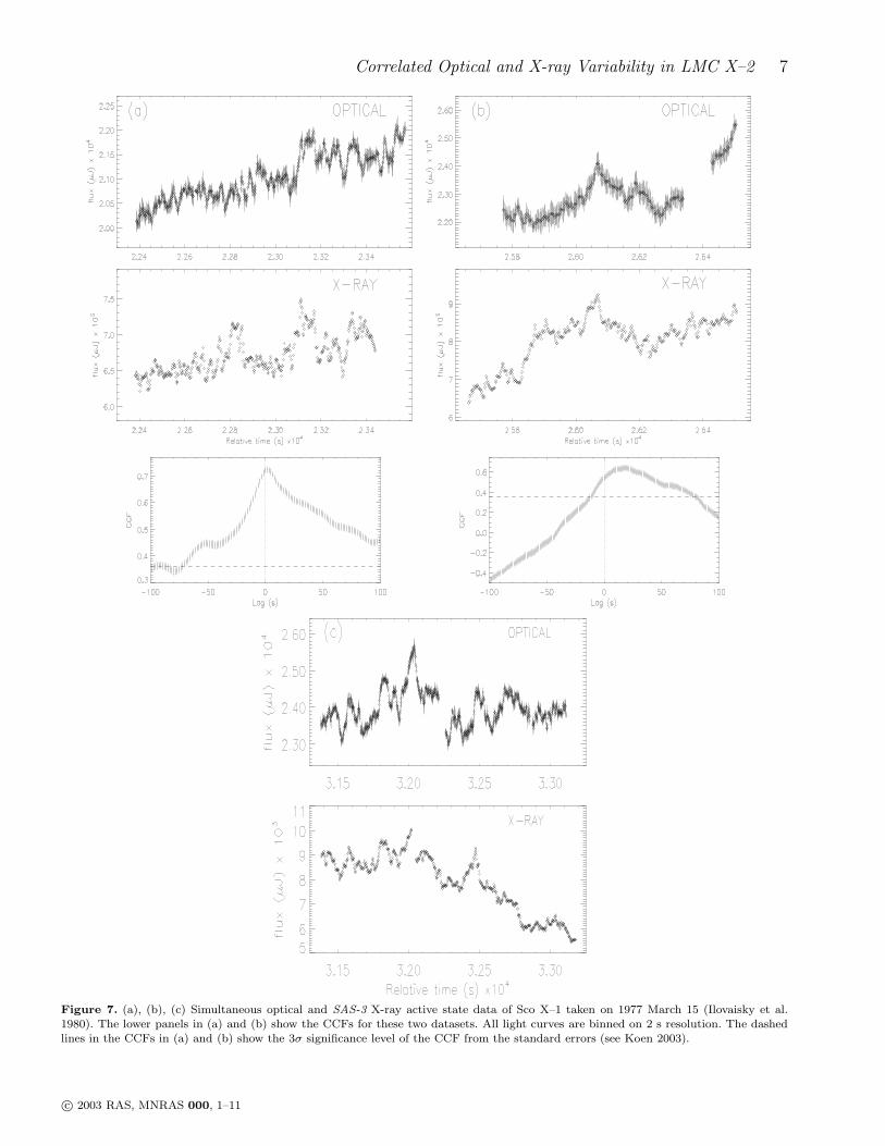
It is instructive to compare LMC X–2’s behaviour with thatof the brightest galactic LMXB, Sco X–1. Ilovaisky et al.(1980; hereafter I80) studied the correlation of variabilityin simultaneous optical and X-ray observations of Sco X–1 using SAS-3, Copernicus and conventional photoelectricphotometry. As we have found with LMC X–2, I80 only de-tected correlated variability occurring when the source wasin a bright, active X-ray state (Fig. 7), with the correlationdecreasing as Sco X–1 became less active. More interestingly,they also found that the peak in their cross-correlation curvegave a delay which was consistent with the optical being de-layed with respect to the X-rays. They attributed this delayto reprocessing of the X-rays in the binary system. Fromtheir observations during a period of high activity they sug-gested that the optical features were delayed by ∼ 30 s com-pared with those in the X-rays. From their cross-correlationanalysis for those data when Sco X–1 was in an active statethey found a range of values for the delay from a few sec-onds to a few tens of seconds. The peak value for the cross-correlation function (CCF) at these delays was not muchgreater than that for zero lag and so they concluded thatthe delays were not very significant.

Petro et al. (1981; hereafter P81) also found correlatedvariability in Sco X–1. Their analysis suggested an opticalsmearing timescale (’filter’ or ’processing’ time) of ∼ 20 s,describing the optical flares as ’filtered’ versions of the X-rayflares. They concluded that the delay could not be due toreprocessing on the secondary as this required a timescaleof only ∼ 10 s, and therefore could not explain the presenceof the long smearing timescale for the system. From therise times of the correlated optical and X-ray flares theyalso concluded that the reprocessing site that produced theoptical flares must be in a different region from the site ofX-ray production (c.f. Pedersen et al. 1982).

c© 2003 RAS, MNRAS 000, 1–11


Figure 5. Left panels, soft (2–4 keV) (first) and hard (4–10 keV) (second) X-ray light curves of LMC X–2, hardness ratio (third), definedas (hard)/(soft). Right panels, the CCFs for the soft (first) and hard light curves (second). Sign convention is such that positive lagscorrespond to X-rays leading the optical. The dashed lines show the 3σ significance level of the CCF from the standard errors (see Koen2003).

Figure 6. Best-fitting predicted light curves (thick line) using a Gaussian transfer function on the two X-ray bands of LMC X–2,2–10 keV (top) and 4–10 keV (bottom). The resulting curves are superimposed on the optical light curve which has been binned on 16 sfor clarity.

c© 2003 RAS, MNRAS 000, 1–11


Figure 7. (a), (b), (c) Simultaneous optical and SAS-3 X-ray active state data of Sco X–1 taken on 1977 March 15 (Ilovaisky et al.1980). The lower panels in (a) and (b) show the CCFs for these two datasets. All light curves are binned on 2 s resolution. The dashedlines in the CCFs in (a) and (b) show the 3σ significance level of the CCF from the standard errors (see Koen 2003).

c© 2003 RAS, MNRAS 000, 1–11


Following our analysis above of LMC X–2, we decidedto investigate such previous X-ray/optical observations ofLMXB’s in greater detail.

4.1 Cross-correlation

We digitized the active state optical and X-ray data ofSco X–1 from I80, converting the data to µJy. We then per-formed cross-correlations of the simultaneous data as havebeen done for LMC X–2 (Fig. 7). We find that the delays forthe first two sets of data are ∼ 1.7±0.9 s and 17.6±5.4 s. Thesignificance of both CCF peaks is > 4σ. The results indicatethat a lag of zero is not ruled out at the 2σ level for the firstset of data, for the second set there is > 3σ confidence of anon-zero lag. For the third set of data no significant delay isfound, but note the decline in the X-rays compared to theconstant optical. The lack of a delay for the second half ofthe data demonstrates again that the X-rays must be in anactive state (i.e. with flaring) to show correlated variabilitywith the optical data.

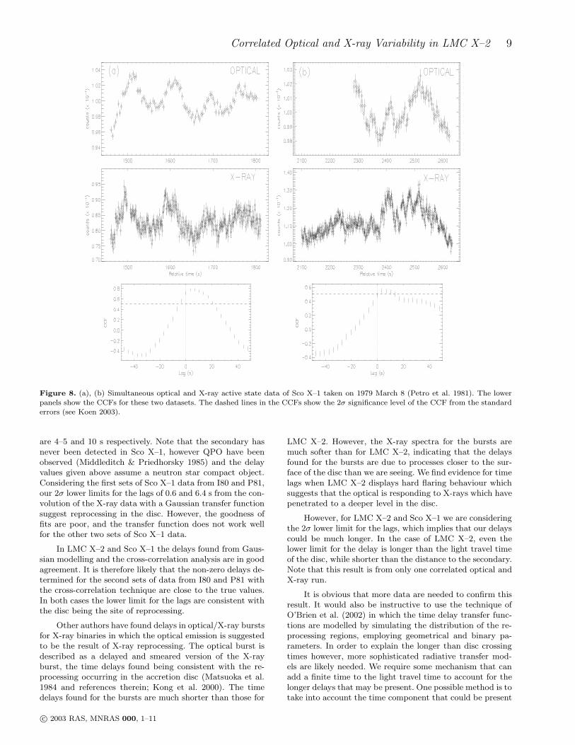
We cross-correlated the two simultaneous active statedatasets from P81, finding delays of 5.9±2.5 s and 5.7±2.8 s(Fig. 8). There is evidence for a non-zero lag in both datasetsat the > 2σ level.

As in LMC X–2, Sco X–1 exhibits an increase in cor-relation between the optical and the X-rays as the sourcebecomes more active. I80 suggested that this could be dueto either one or two regions of optical emission. In the caseof one optical emitting zone, they suggested that the opti-cal reprocessing region is illuminated by the X-ray sourceat all times, but ’something’ is required to damp out theX-ray variability between the compact object and the ob-server when the source is in a non-active state, or perhapsthe optical “region” cannot then see the X-rays. For the caseof two emitting regions, they suggest that the uncorrelatedemission (∼ 25% less energetic in the X-rays than duringcorrelated emission) could be due to optical emission fromthe disc itself, while the correlated emission could be due toX-ray heating of different parts of the system and would bedirectly related to the X-ray emission.

The lags determined from the cross-correlation analysisagain represent the characteristic delay present between theoptical and X-ray light curves. In order to model the timedelay we have also convolved the X-ray light curves of Sco X–1 from I80 and P81 with a Gaussian transfer function, as hasbeen done for LMC X–2 (see Section 3.2).

4.2 Transfer Function

A series of convolutions of the transfer function with eachof the X-ray light curves were performed on the first twodatasets from I80 (Fig 7 (a) and (b)), and both sets of datafrom P81 (Fig 8 (a) and (b)). Again both τ0 and ∆τ werevaried independently. The results of fitting the Gaussiantransfer functions to the Sco X–1 X-ray data are summa-rized in Table 3. The values of χ2

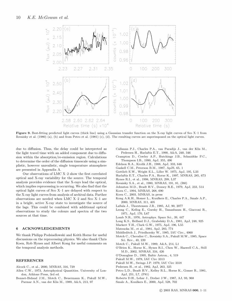
ν indicate that the fits arenot good. The best-fitting predicted light curves from theconvolutions superimposed on the optical light curves areshown in Fig 9.

The predicted light curves reproduce the optical datamarginally for the first set of I80 data and the first set of

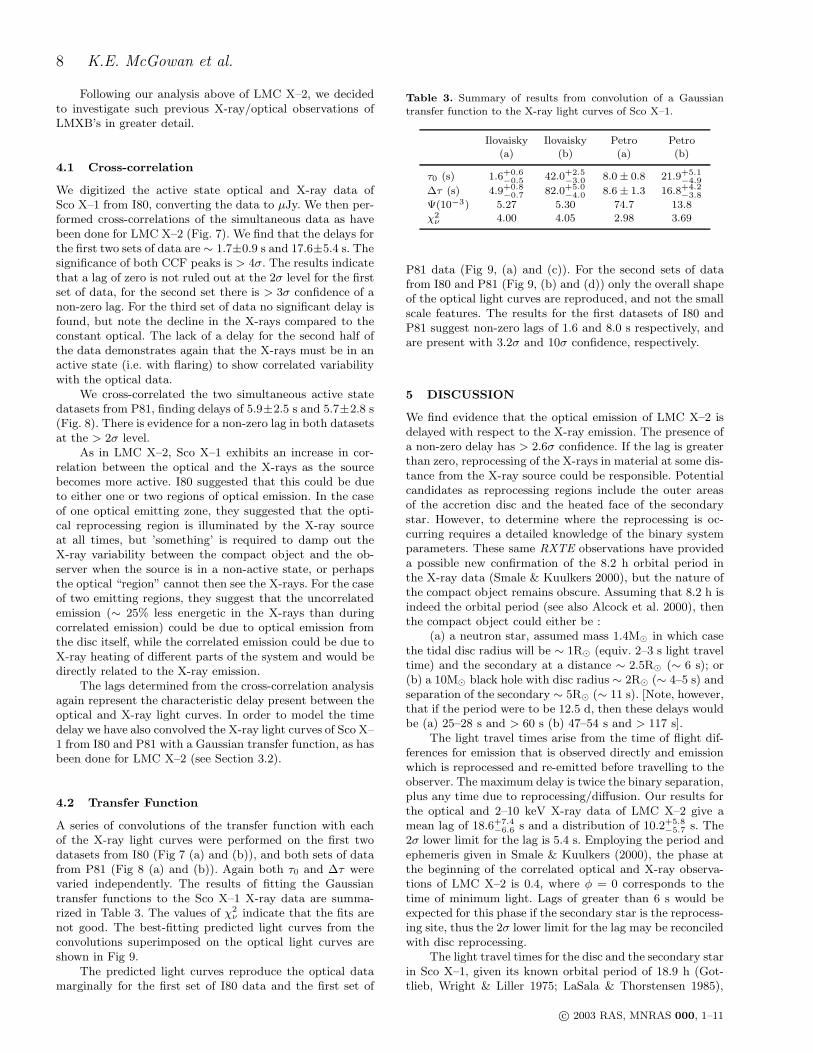
Table 3. Summary of results from convolution of a Gaussiantransfer function to the X-ray light curves of Sco X–1.

Ilovaisky Ilovaisky Petro Petro(a) (b) (a) (b)

τ0 (s) 1.6+0.6−0.5 42.0+2.5

−3.0 8.0 ± 0.8 21.9+5.1−4.9

∆τ (s) 4.9+0.8−0.7 82.0+5.0

−4.0 8.6 ± 1.3 16.8+4.2−3.8

Ψ(10−3) 5.27 5.30 74.7 13.8

χ2ν 4.00 4.05 2.98 3.69

P81 data (Fig 9, (a) and (c)). For the second sets of datafrom I80 and P81 (Fig 9, (b) and (d)) only the overall shapeof the optical light curves are reproduced, and not the smallscale features. The results for the first datasets of I80 andP81 suggest non-zero lags of 1.6 and 8.0 s respectively, andare present with 3.2σ and 10σ confidence, respectively.

5 DISCUSSION

We find evidence that the optical emission of LMC X–2 isdelayed with respect to the X-ray emission. The presence ofa non-zero delay has > 2.6σ confidence. If the lag is greaterthan zero, reprocessing of the X-rays in material at some dis-tance from the X-ray source could be responsible. Potentialcandidates as reprocessing regions include the outer areasof the accretion disc and the heated face of the secondarystar. However, to determine where the reprocessing is oc-curring requires a detailed knowledge of the binary systemparameters. These same RXTE observations have provideda possible new confirmation of the 8.2 h orbital period inthe X-ray data (Smale & Kuulkers 2000), but the nature ofthe compact object remains obscure. Assuming that 8.2 h isindeed the orbital period (see also Alcock et al. 2000), thenthe compact object could either be :

(a) a neutron star, assumed mass 1.4M⊙ in which casethe tidal disc radius will be ∼ 1R⊙ (equiv. 2–3 s light traveltime) and the secondary at a distance ∼ 2.5R⊙ (∼ 6 s); or(b) a 10M⊙ black hole with disc radius ∼ 2R⊙ (∼ 4–5 s) andseparation of the secondary ∼ 5R⊙ (∼ 11 s). [Note, however,that if the period were to be 12.5 d, then these delays wouldbe (a) 25–28 s and > 60 s (b) 47–54 s and > 117 s].

The light travel times arise from the time of flight dif-ferences for emission that is observed directly and emissionwhich is reprocessed and re-emitted before travelling to theobserver. The maximum delay is twice the binary separation,plus any time due to reprocessing/diffusion. Our results forthe optical and 2–10 keV X-ray data of LMC X–2 give amean lag of 18.6+7.4

−6.6 s and a distribution of 10.2+5.8−5.7 s. The

2σ lower limit for the lag is 5.4 s. Employing the period andephemeris given in Smale & Kuulkers (2000), the phase atthe beginning of the correlated optical and X-ray observa-tions of LMC X–2 is 0.4, where φ = 0 corresponds to thetime of minimum light. Lags of greater than 6 s would beexpected for this phase if the secondary star is the reprocess-ing site, thus the 2σ lower limit for the lag may be reconciledwith disc reprocessing.

The light travel times for the disc and the secondary starin Sco X–1, given its known orbital period of 18.9 h (Got-tlieb, Wright & Liller 1975; LaSala & Thorstensen 1985),

c© 2003 RAS, MNRAS 000, 1–11


Figure 8. (a), (b) Simultaneous optical and X-ray active state data of Sco X–1 taken on 1979 March 8 (Petro et al. 1981). The lowerpanels show the CCFs for these two datasets. The dashed lines in the CCFs show the 2σ significance level of the CCF from the standarderrors (see Koen 2003).

are 4–5 and 10 s respectively. Note that the secondary hasnever been detected in Sco X–1, however QPO have beenobserved (Middleditch & Priedhorsky 1985) and the delayvalues given above assume a neutron star compact object.Considering the first sets of Sco X–1 data from I80 and P81,our 2σ lower limits for the lags of 0.6 and 6.4 s from the con-volution of the X-ray data with a Gaussian transfer functionsuggest reprocessing in the disc. However, the goodness offits are poor, and the transfer function does not work wellfor the other two sets of Sco X–1 data.

In LMC X–2 and Sco X–1 the delays found from Gaus-sian modelling and the cross-correlation analysis are in goodagreement. It is therefore likely that the non-zero delays de-termined for the second sets of data from I80 and P81 withthe cross-correlation technique are close to the true values.In both cases the lower limit for the lags are consistent withthe disc being the site of reprocessing.

Other authors have found delays in optical/X-ray burstsfor X-ray binaries in which the optical emission is suggestedto be the result of X-ray reprocessing. The optical burst isdescribed as a delayed and smeared version of the X-rayburst, the time delays found being consistent with the re-processing occurring in the accretion disc (Matsuoka et al.1984 and references therein; Kong et al. 2000). The timedelays found for the bursts are much shorter than those for

LMC X–2. However, the X-ray spectra for the bursts aremuch softer than for LMC X–2, indicating that the delaysfound for the bursts are due to processes closer to the sur-face of the disc than we are seeing. We find evidence for timelags when LMC X–2 displays hard flaring behaviour whichsuggests that the optical is responding to X-rays which havepenetrated to a deeper level in the disc.

However, for LMC X–2 and Sco X–1 we are consideringthe 2σ lower limit for the lags, which implies that our delayscould be much longer. In the case of LMC X–2, even thelower limit for the delay is longer than the light travel timeof the disc, while shorter than the distance to the secondary.Note that this result is from only one correlated optical andX-ray run.

It is obvious that more data are needed to confirm thisresult. It would also be instructive to use the technique ofO’Brien et al. (2002) in which the time delay transfer func-tions are modelled by simulating the distribution of the re-processing regions, employing geometrical and binary pa-rameters. In order to explain the longer than disc crossingtimes however, more sophisticated radiative transfer mod-els are likely needed. We require some mechanism that canadd a finite time to the light travel time to account for thelonger delays that may be present. One possible method is totake into account the time component that could be present

c© 2003 RAS, MNRAS 000, 1–11


Figure 9. Best-fitting predicted light curves (thick line) using a Gaussian transfer function on the X-ray light curves of Sco X–1 fromIlovaisky et al. (1980) (a), (b) and from Petro et al. (1981) (c), (d). The resulting curves are superimposed on the optical light curves.

due to diffusion. Thus, the delay could be interpreted asthe light travel time with an added component due to diffu-sion within the absorption/re-emission region. Calculationsto determine the order of the diffusion timescale using a sim-plistic, however unrealistic, single temperature atmosphereare presented in Appendix A.

Our observations of LMC X–2 show the first correlatedoptical and X-ray variability for the source. The temporalanalysis provides evidence that the X-rays lead the optical,which implies reprocessing is occurring. We also find that theoptical light curves of Sco X–1 are delayed with respect tothe X-ray light curves from analysis of archival data. Furtherobservations are needed when LMC X–2 and Sco X–1 arein a bright, active X-ray state to investigate the source ofthe lags. This could be combined with additional opticalobservations to study the colours and spectra of the twosources at that time.

6 ACKNOWLEDGEMENTS

We thank Philipp Podsiadlowski and Keith Horne for usefuldiscussions on the reprocessing physics. We also thank ChrisKoen, Rob Hynes and Albert Kong for useful comments onthe temporal analysis methods.

REFERENCES

Alcock C., et al., 2000, MNRAS, 316, 729Allen C.W., 1973, Astrophysical Quantities. University of Lon-

don, Athlone Press, 3rd ed.Bonnet-Bidaud J.M., Motch C., Beuermann K., Pakull M.W.,

Parmar A.N., van der Klis M., 1989, A&A, 213, 97

Callanan P.J., Charles P.A., van Paradijs J., van der Klis M.,Pedersen H., Harlaftis E.T., 1990, A&A, 240, 346

Crampton D., Cowley A.P., Hutchings J.B., Schmidtke P.C.,Thompson I.B., 1990, ApJ, 355, 496

Edelson R.A., Krolik J.H., 1988, ApJ, 333, 646Gaskell C.M., Peterson B.M., 1987, ApJS, 65, 1

Gottlieb E.W., Wright E.L., Liller W. 1975, ApJ, 195, L33Harlaftis E.T., Charles P.A., Horne K., 1997, MNRAS, 285, 673Hynes R.I., et al., 1998, MNRAS, 299, L37

Ilovaisky S.A., et al., 1980, MNRAS, 191, 81, (I80)Johnston M.D., Bradt H.V., Doxsey R.E., 1979, ApJ, 233, 514

Koen C., 1994, MNRAS, 268, 690Koen C., 2003, MNRAS, in pressKong A.K.H., Homer L., Kuulkers E., Charles P.A., Smale A.P.,

2000, MNRAS, 311, 405

LaSala J., Thorstensen J.R., 1985, AJ, 90, 2077Leong C., Kellog E., Gursky H., Tananbaum H., Giacconi R.,

1971, ApJ, 170, L67

Lomb N.R., 1976, Astrophys. Space Sci., 39, 447Long K.S., Helfand D.J., Grabelsky D.A., 1981, ApJ, 248, 925Markert T.H., Clark G.W., 1975, ApJ, 196, L55

Matsuoka M., et al., 1984, ApJ, 283, 774Middleditch J., Priedhorsky W., 1985, IAU Circ., 4060Motch C., Chevalier C., Ilovaisky S.A., Pakull M.W., 1985, Space

Sci. Rev., 40, 239

Motch C., Pakull M.W., 1989, A&A, 214, L1O’Brien K., Horne K., Hynes R.I., Chen W., Haswell C.A., Still

M.D., 2002, MNRAS, 334, 426

O’Donoghue D., 1995, Baltic Astron., 4, 519Pakull M.W., 1978, IAU Circ 3313Pakull M.W., Swings J.P. 1979, IAU Circ 3318

Pedersen H., et al., 1982, ApJ, 263, 325Petro L.D., Bradt H.V., Kelley R.L., Horne K., Gomer R., 1981,

ApJ, 251, L7, (P81)Roberts D.H., Lehar J., Dreher J.W., 1987, AJ, 93, 968

Smale A., Kuulkers E., 2000, ApJ, 528, 702

c© 2003 RAS, MNRAS 000, 1–11


Stetson P.B., 1987, PASP, 99, 191

van Paradijs J., 1983, in Accretion-Driven Stellar X-ray Sources,ed. Lewin, van den Heuvel, 189, Cambridge University Press,Cambridge

Webbink R.F., Rappaport S., Savonije G.J., 1983, ApJ, 270, 678White N.E., 1989, Astron. Ast. Rev., 1, 85

APPENDIX A: DIFFUSION TIMESCALE

CALCULATIONS

Using a simple model for the secondary star or the ’atmo-sphere’ of the disc, we can estimate the duration of the diffu-sion timescale, the time it takes for the X-ray photons to beabsorbed and the energy deposited there to be re-emittedin the optical. This timescale is heavily dependent on thedensity and opacity of the star/disc.

Assume the X-rays penetrate to a depth d in the pho-tosphere where κx is X-ray opacity (κx = 0.2(1 +X) ∼ 0.34cm2g−1) and ρ is density, then

d ∼ 1

κxρ(A1)

The number of scatterings is then ∼ (dκ◦ρ)2 where κ◦ is

the optical opacity, and the time between each scattering is∼ 1/(κ◦ρc). Combining these with Eq. A1 we can define thediffusion timescale as

tdiff =(

κ◦

κx

)2

· 1

κ◦ρc(A2)

From the equations for the optical depth and pressure of thephotosphere, assuming that κ◦ is constant in depth d, andthat the gravity g remains roughly constant over d, then wecan derive an expression for κ◦ (assuming an ideal gas)

κ◦

g=

2

3

kµH mH

ρTeff

(A3)

Replacing g in Eq. A3 with GM/R2 and rearranging to getan expression for κ◦ρ we can substitute this into Eq. A2 togive

tdiff =(

κ◦

κx

)2

·

[

3

2· kTeff

µH mH

GMR

· Rc

]

(A4)

By calculating the irradiating flux (Fx) we can derive theirradiation temperature Tx, given by

Tx =(

fFx

2σ

)1/4

(A5)

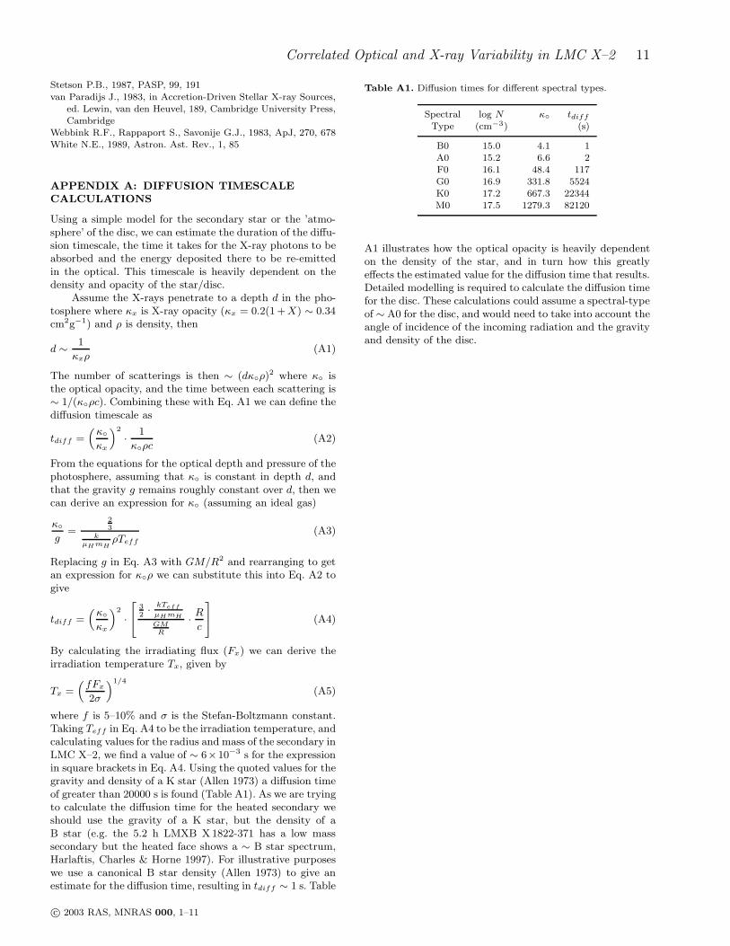
where f is 5–10% and σ is the Stefan-Boltzmann constant.Taking Teff in Eq. A4 to be the irradiation temperature, andcalculating values for the radius and mass of the secondary inLMC X–2, we find a value of ∼ 6×10−3 s for the expressionin square brackets in Eq. A4. Using the quoted values for thegravity and density of a K star (Allen 1973) a diffusion timeof greater than 20000 s is found (Table A1). As we are tryingto calculate the diffusion time for the heated secondary weshould use the gravity of a K star, but the density of aB star (e.g. the 5.2 h LMXB X1822-371 has a low masssecondary but the heated face shows a ∼ B star spectrum,Harlaftis, Charles & Horne 1997). For illustrative purposeswe use a canonical B star density (Allen 1973) to give anestimate for the diffusion time, resulting in tdiff ∼ 1 s. Table

Table A1. Diffusion times for different spectral types.

Spectral log N κ◦ tdiff

Type (cm−3) (s)

B0 15.0 4.1 1A0 15.2 6.6 2F0 16.1 48.4 117G0 16.9 331.8 5524K0 17.2 667.3 22344M0 17.5 1279.3 82120

A1 illustrates how the optical opacity is heavily dependenton the density of the star, and in turn how this greatlyeffects the estimated value for the diffusion time that results.Detailed modelling is required to calculate the diffusion timefor the disc. These calculations could assume a spectral-typeof ∼ A0 for the disc, and would need to take into account theangle of incidence of the incoming radiation and the gravityand density of the disc.

c© 2003 RAS, MNRAS 000, 1–11

Correlated Optical and X-ray Variability in LMC X-2

Documents