Correlated Equilibria in Voter Turnout Games

Correlated Equilibria in Voter Turnout Games

Kirill Pogorelskiy∗

Job Market Paper

December 15, 2014

Abstract

Communication is fundamental to elections. This paper extends canonical voter turnout models

to include any form of communication, and characterizes the resulting set of correlated equilibria. In

contrast to previous research, high-turnout equilibria exist in large electorates and uncertain environ-

ments. This difference arises because communication can be used to coordinate behavior in such a way

that voters find it incentive compatible to always follow their signals past the communication stage.

The equilibria have expected turnout of at least twice the size of the minority for a wide range of

positive voting costs, and show intuitive comparative statics on turnout: it varies with the relative

sizes of different groups, and decreases with the cost of voting. This research provides a general micro

foundation for group-based theories of voter mobilization, or voting driven by communication on a

network.

Keywords: turnout paradox, rational voting, correlated equilibrium, group-based voter mobiliza-

tion, pre-play communication

JEL codes: C72, D72

1 Introduction

What drives voter turnout is a fundamental question in political economy. Canonical models, which

rely on voters rationally and independently deciding whether to turn out based on how likely they are

to be pivotal to the election outcomes, provide unsatisfactory explanations (Downs (1957), Riker and

Ordeshook (1968), Palfrey and Rosenthal (1985), Myerson (2000)). In particular, these models fail to

rationalize the high turnout rates observed in very large elections. Intuitively, as the electorate grows

large, the probability that any individual voter is pivotal goes to zero, so with voting incurring a cost, very

few people should turn out. This flaw has led many scholars to seek alternative, behavioral explanations

(Feddersen and Sandroni (2006), Bendor et al. (2011), Ali and Lin (2013)).

∗Division of the Humanities and Social Sciences, MC 228-77, California Institute of Technology, Pasadena, CA 91125.Email: [email protected]. Web: hss.caltech.edu/kbp

First draft: February 2013. I am indebted to Tom Palfrey for guidance and encouragement. I thank Marina Agranov,R. Michael Alvarez, Kim Border, Laurent Bouton, Federico Echenique, Matt Elliott, Alexander Hirsch, John Ledyard,Priscilla Man, Francesco Nava, Salvatore Nunnari, Yuval Salant, Erik Snowberg, and Leeat Yariv for insightful commentsand discussions. I thank Erik Snowberg for helping me improve my writing style. I thank Jean-Laurent Rosenthal and theaudience of the pro-seminar at Caltech, Leslie Johns and participants of the UCLA workshop, conference participants at the2014 meetings of the Midwest Political Science Association, Society for Social Choice and Welfare, North American SummerMeeting of the Econometric Society, the American Political Science Association, and seminar participants at Princeton,Texas A&M, and UC San Diego.

1

http://hss.caltech.edu/kbp

This paper re-examines these results in the presence of communication, broadly defined – between

candidates, media, and voters – and shows that this can support high turnout in large elections while

maintaining the assumption that voters’ incentives are purely instrumental. The key difference is that

communication allows for strategies such that equilibrium behavior is still optimal for each individual

voter, but such that voters’ turnout decisions are now correlated, rather than independent as in the

standard game-theoretic analysis. That is, communication allows us to examine correlated equilibria

(Aumann, 1974, 1987). These equilibria are behaviorally more realistic than Nash since they do not

require voters to know for sure the strategies of every other voter, and so can apply to electorates with

less than fully informed voters, like the U.S. (Bartels, 1996).

As suggested above, the forms of communication allowed in the model are extremely general. The

only necessary condition is that the communication can result in some amount of correlation in voters’

decisions. As such, the model provides a very rich space in which communication can be from a few

senders to many receivers – as it would be with the media or parties communicating with voters – or

between a very large number of senders and receivers. In this sense, the model can provide a micro-

foundation for group-based voter mobilization: as mobilization efforts induce correlation in decisions,

they provide a mechanism for turnout that does not rely on group-based utilities or coercion (Uhlaner

(1989), Schram and van Winden (1991), Cox (1999)). Moreover, as correlation could be induced by any

signal – even signals like weather, which would not be thought of as having political content – the model

incorporates mechanisms that would not play any role in standard rational choice explanations.1

The intuition underlying the highest-turnout correlated equilibrium is straightforward. To see this,

suppose there are two parties, A and B, who compete in an election decided by majority rule. Citizens

(potential voters) are not indifferent between the parties, so there are nA citizens that support party A and

nB < nA citizens that support party B. Each citizen decides to vote based only on the tradeoff between

her potential effect on the election outcome and the cost of voting. A voter will only affect the outcome

when pivotal, that is, when her vote would change the election from her least favored party winning to

a tie, or from a tie to her most favored party winning. As in standard models, in any equilibrium, the

probability that a voter is pivotal, multiplied by the benefit she gets from changing the outcome of the

election, must be greater than or equal to the cost of voting. Thus turnout is highest when the election

results in a tie, either directly or in expectation.

Without communication, citizens will make turnout decisions independently. The largest tie would

require all of minority citizens (nB citizens), and the exact same number of majority citizens (nB out

of nA citizens) to participate. In such a case, every recruited citizen would be pivotal with the same

probability, and so, as long as it is high enough, would have incentives to turn out as required by this

strategy. But the remaining nA − nB majority citizens would deviate by also turning out, so this is not

an equilibrium. In fact, except for few very special cases, there are no equilibria where all citizens use

deterministic (i.e., pure) strategies.

With communication, however, turnout decisions can be correlated. The party supported by the

minority of the citizens signals all of its supporters to vote. The party with the majority support uses a

more complicated communication protocol.2 In some fraction of elections, p, the majority party creates a

1See Gomez, Hansford, and Krause (2007) who demonstrate not only that the bad weather on the election day decreasesturnout, but also that it affects Democrats and Republicans differently.

2I thank the anonymous referee for suggesting the idea of this example.

2

pivotal situation by sending a signal to vote to nB of its supporters and no signal to the rest of majority

citizens. In the remaining fraction of elections, the majority party sends to all of its supporters a signal

to vote with probability nBnA

, and no signal with probability 1− nBnA

. Therefore, each minority citizen will

be pivotal with probability p. As long as p is high enough, all minority citizens will find it in their interest

to turn out and vote. On the other hand, the majority citizens, based on the signal from their party, will

not know for sure whether or not they are in the pivotal situation. For the value of p corresponding to

the correlated equilibrium, majority citizens will also find it in their interest to follow the signal of their

party, and to avoid the cost of voting by abstaining if they receive no signal. It is easy to see that in

this correlated equilibrium the expected turnout will be quite high: twice the size of the minority. If the

minority is large enough, voter turnout could thus be close to 100%.

The upper bound on turnout of twice the size of the minority, highlighted in the example above,

is sometimes closely approached by the actual elections. To take a recent high profile elections, the

2014 referendum on Scottish independence gathered 1,617,989 votes in favor of independence.3 Internet,

telephone, and face-to-face opinion polls, averaged over the last two months before the referendum day

indicated that about 42.07% of Scots supported independence, which translates into about 1,802,023

citizens.4 Assuming that polls more or less perfectly revealed the majority and minority supports, this

means that nearly 90% of minority citizens turned out, which is close to the full minority turnout in the

example. Moreover, the total turnout was 3,619,915 citizens, which is almost exactly twice the size of

the minority (up to a third decimal point).

The remainder of the paper is organized as follows. Subsection 1.1 provides a literature overview.

Section 2 describes the basic model, which assumes complete information and homogenous voting costs.

Subsections 2.1.1 and 2.1.2 present and discuss the main results for this case. Subsection 2.1.3 presents

efficiency analysis for the basic model. Section 3 extends the basic model to the case of heterogeneous

voting costs and shows that the main results continue to hold. Section 4 explores the effects of private

information about voting costs and relative party sizes. Section 5 discusses how our results extend the

related findings in the existing literature. Section 6 concludes.

1.1 Related Literature

Our paper directly relates to two strands of the voluminous literature on formal models of turnout. One

is the pivotal voter model, in particular, Palfrey and Rosenthal (1983, 1985). The other is group-based

models that build upon the pivotal voter analysis, e.g. Morton (1991). Our model combines these

approaches, and so contributes to the literatures on the turnout paradox and voter mobilization.

The turnout paradox, that is, the unsupportable rational choice prediction of turnout rate close

to zero in large elections, was first formulated by Downs (1957) in the context of a decision theoretic

voting model, which was extended later by Tullock (1967) and Riker and Ordeshook (1968). It would

be impossible to mention here all the relevant papers that have been published on the topic since those

early studies, so we have to restrict ourselves to the most closely related works. We refer the reader to

Feddersen (2004) and Geys (2006) for very well-written recent literature surveys. See also Palfrey (2013)

for a recent survey of laboratory experiments in political economy, including experiments testing different

3Source: www.bbc.com/news/events/scotland-decides/results4Source: whatscotlandthinks.org/questions/should-scotland-be-an-independent-country-1

3

http://www.bbc.com/news/events/scotland-decides/results

http://whatscotlandthinks.org/questions/should-scotland-be-an-independent-country-1

theories of turnout (Ibid., Section 4).

The pivotal voter model of Palfrey and Rosenthal (1983) argues that voters’ decisions to turn out are

strategic, so the probability of being pivotal must be determined endogenously in equilibrium. Under

complete information and common voting cost, Palfrey and Rosenthal (1983) found several classes of

high-turnout Nash equilibria. Under incomplete information about voting costs, though, Palfrey and

Rosenthal (1985) showed that non-zero turnout rate in large elections is not sustainable in the (quasi-

symmetric) Bayesian Nash equilibrium: only voters with non-positive voting costs will vote in the limit

as the majority and minority groups get large. Myerson (1998, 2000) introduced a very general approach

to the analysis of large games with population uncertainty. However his “independent actions property”

assumption, which results in the number of players being a Poisson random variable, does not allow

correlation between players’ strategies. Barelli and Duggan (2013) prove existence of a pure strategy

Bayesian Nash equilibrium in games with correlated types and interdependent payoffs. Their Example

2.4, an application of their main purification theorem, is a more general version of the costly voting game

under incomplete information than the one we consider in Section 4. Unlike them, we study the strategic

form correlated equilibria of this game that differ from Bayesian Nash equilibria with correlated types,

and focus on characterizing the bounds on expected turnout rather than equilibrium existence.

Although the pivotal voter model prediction about expected turnout fails under incomplete informa-

tion, the comparative static predictions are largely supported in laboratory experiments: see, e.g. Levine

and Palfrey (2007) and Grosser and Schram (2010). More recent work falling within this approach fo-

cused on welfare effects associated with turnout, comparison of mandatory and voluntary voting rules,

and the effect of polls (e.g. Borgers (2004), Goeree and Grosser (2007), Diermeier and Van Mieghem

(2008), Krasa and Polborn (2009), Taylor and Yildirim (2010)). Campbell (1999) finds that decisive

minorities (i.e., those with lower voting costs or with greater expected benefits) are more likely to win in

a quasi-symmetric equilibrium, even if their expected share in the electorate is small. His main point of

departure from Palfrey and Rosenthal (1985) is introducing correlation between voter types (i.e., party

preference) and voting cost. In this respect, he extends Ledyard (1984) who assumed that types and

costs are distributed independently.

Kalandrakis (2007, 2009) looks at general turnout games with complete information and heteroge-

neous costs, and shows that almost all Nash equilibria of these games are regular and robust to small

amounts of incomplete information. These findings can be compared to our results in Sections 3 and 4.

Another closely related paper is Myatt (2012), who investigates how adding aggregate uncertainty about

candidates’ popularity could be used to solve the turnout paradox. His main result can be viewed as

adding a modicum of correlation in an asymptotic approximation of the high-turnout quasi-symmetric

Nash equilibrium characterized in Palfrey and Rosenthal (1985) to rule out zero equilibrium turnout as

the electorate grows large. Similarly to those equilibria, it requires the common voting cost to be high

enough, and predicts a tie in the equilibrium. Myatt (2012, Proposition 2) shows that the same logic can

be applied to mixed-pure Nash equilibria, but characterizes the expected turnout only for a special case

of the candidates’ popularity density. Our results allow for correlation directly in the solution concept.

There are other prominent approaches to modeling voter behavior that aim at solving the turnout

paradox (e.g., ethical voter models of Feddersen and Sandroni (2006), and Coate and Conlin (2004); see

also the recent extensions by Evren (2012) and Ali and Lin (2013); or adaptive learning models, e.g.,

4

Bendor et al. (2011); or models based on uncertainty about candidates, e.g. Sanders (2001), or the quality

of voters’ private signals, e.g. McMurray (2013)). While these and similar models highlight a number of

important aspects of voting in mass elections, by the very same way of being tied to the voting context,

they are a bit limited in scope. Our approach in this paper is kind of the opposite: we deliberately

abstract from the context as much as possible to show that even in this stark setting the high turnout

equilibria can be supported.5

Unlike the pivotal voter model, where the individual voter is a central unit of analysis, group-based

models operate at the level of groups of voters. An early example is Becker (1983), who models competi-

tion among pressure groups for political influence non-strategically as independent utility maximization

by each group subject to a joint budget constraint. Uhlaner (1989) emphasizes the role of groups in voting

decisions, but does not characterize the equilibrium of the model. Morton (1991) shows that with fixed

candidates’ positions, positive turnout can be obtained in equilibrium with two groups, but in the general

equilibrium framework, where candidates’ positions can shift, the paradox prevails. Schram (1991) and

Schram and van Winden (1991) develop a model with two groups and opinion leaders in each group, who

produce social pressure on others to turn out. The individual voters are modeled as consumers of social

pressure. It is shown that it is optimal for the producers of social pressure to do it, however, to explain

why consumers of social pressure would find it optimal to follow the leaders, a civic duty argument is

used. Shachar and Nalebuff (1999) develop a model of a pivotal leader, and structurally estimate it using

voting data for U.S. presidential elections. See Rosenstone and Hansen (1993), Cox (1999), and references

therein for an overview of empirical findings related to party mobilization models.

Overall, group-based models get around the turnout paradox by assuming the existence of a small

number of group leaders who control voter mobilization decisions by allocating resources or by means of

social pressure. The exogenous mapping from mobilization efforts to voter turnout is assumed. The micro

foundation for the control mechanism as well as the origins of group leaders are not usually modeled. In

our case, both of these mechanisms arise naturally as coordination mechanisms in the form of pre-play

communication among voters. Communication in turn induces correlation among the voters’ strategies

that can lead to surprisingly high turnout.

There is growing field and laboratory experimental evidence that communication among voters, and

between political activists and voters, taken in a wide variety of forms (e.g., public opinion polls, get-out-

the-vote campaigns, and so forth) critically influences turnout rates. A book-length treatment of field

experiments studying effects of get-out-the-vote campaigns on turnout is Gerber and Green (2008), and

one of influential earlier papers is Gerber and Green (2000). Gerber et al (2011) show that effects of TV

advertising may be strong but short-lived. See also Lassen (2005) on a related topic of voter information

affecting turnout.6 Recently, DellaVigna et al (2014) emphasize the social pressure aspect of turnout,

also studied in Gerber, Green, and Larimer (2008), while Barber and Imai (2014) show that even the

neighborhood composition itself may matter for turnout. A recent work by Sinclair (2012) emphasizes

the role of networks in political behavior, arguing that networks not only provide information, but also

5One way to compare turnout theories that make similar predictions is to try to recover concealed parameter values ofdifferent models from the same data set and see if the results are comparable and plausible. Using the lab experiment datafrom Levine and Palfrey (2007), Merlo and Palfrey (2013) find less support for the ethical voter model of Coate and Conlin(2004), compared to other turnout models.

6McMurray (2012) notes that models that avoid the turnout paradox by introducing consumption benefits, at the sametime nullify the empirical relation between voter information and turnout.

5

directly influence citizens’ actions. See also Rolfe (2012). This approach is complementary to our work:

while we do not explicitly model social connections among voters in this paper, one can easily imagine

how such network links could serve as channels of pre-play communication.

Laboratory experiments include, e.g., Grosser and Schram (2006), who study the effects of commu-

nication in the form of neighborhood information exchange between an early voter (sender) and a late

voter (receiver) from the same neighborhood. Grosser and Schram (2010), and Agranov et al. (2013)

study the effects of polls. Goeree and Yariv (2011) investigate communication effects in the jury context

and find that communication has a large effect on observed outcomes.

The effects of communication on turnout may be also indirect. For example, Ortoleva and Snow-

berg (2014) find, inter alia, that voter overconfidence, even conditional on ideology, increases turnout.

Communication among voters might be a possible way that overconfidence builds up in the first place.

2 The Model

The set of voters is denoted N , with |N | = n ≥ 3. There are two candidates, A and B. The decision

making rule is simple majority with ties broken randomly. Each player i ∈ N has type7 ti ∈ {A,B}representing her political preference: if ti = A then i prefers candidate A to candidate B, if ti = B then

the preference is reversed. Denote by NA, with |NA| = nA, the group of voters who prefer candidate

A, and NB, with |NB| = nB, the group preferring candidate B. Throughout the paper we assume that

nA > nB, and will refer to NA and NB as majority and minority, respectively. Thus in the usual parlance,

candidate A is the favorite, while candidate B is the underdog.

Each voter has two pure actions: to vote for the preferred candidate (action 1) or abstain (action

0).8 Thus i’s action space is Si = {0, 1}. The set of voting profiles is S = S1 × · · · × Sn, i.e. S =

{(si)i∈N |si ∈ {0, 1}}. Voting is costly, and utility of voting net of voting cost is normalized to 1 if the

preferred candidate wins, 1/2, if there is a tie, and 0 otherwise. Instead of explicitly modelling candidates

as players of this game, we use a representation with a centralized mediator giving out recommendations

to voters, who either maximizes or minimizes total expected turnout. As will be clear from Proposition

1, our main result, this does not matter for the empirically relevant case of the large minority with

nB > 12nA. In Pogorelskiy (2014) we analyze the general case where this representation matters.

2.1 Complete Information and Homogeneous Voting Costs

In this section we assume that NA and NB are commonly known. Furthermore, assume that the partici-

pation cost is the same for all voters and fixed at c ∈ (0, 1/2).9 In a more general case with heterogeneous

costs, considered in Section 3, we discuss how one could allow some voters, e.g., those who view voting

as a social duty, to have negative voting costs. In the case of a negative common cost, however, letting

c < 0 results in a trivial equilibrium with everybody voting, so for the rest of this section we only consider

non-negative values of c.

7We do not explicitly include i’s private voting cost in her type for convenience reasons and always refer to i’s votingcosts separately.

8Voting for a less preferred candidate is always dominated, and can be dispensed with.9If c ≥ 1

2(c ≤ 0), the problem is trivial, with abstaining (voting) being everyone’s dominant strategy.

6

Definition 1. A correlated equilibrium is a probability distribution10 µ ∈ ∆(S) such that for all i ∈ N ,

for all si ∈ {0, 1}, and all s′i ∈ {0, 1}∑s−i∈S−i

µ(si, s−i)(Ui(si, s−i)− Ui(s′i, s−i)

)≥ 0 (1)

where Ui(si, s−i) is the utility of voter i at a strategy profile (si, s−i).

To get some intuition for this definition, assume for a moment that all joint strategy profiles have

a strictly positive probability, and divide both sides of (1) by Prob(si) =∑

s−i∈S−iµ(si, s−i). Since

Prob(s−i|si) = µ(si, s−i)/Prob(si), correlated equilibrium can be interpreted as a probability distribution

over joint strategy profiles where at every profile player i’s choice is a weak best response under the

posterior distribution conditional on that choice. Conditioning is used here to obtain the others’ posteriors

about player i’s choice, which must be correct in equilibrium. Notice also that Nash equilibrium is a special

case of correlated equilibrium, where µ is the product of n independent probability distributions, each one

over the corresponding player’s action space. Thus Nash equilibrium rules out any correlation between

players’ actions.

Call (1) voter i’s incentive compatibility (IC) constraints. Since each player has only two (pure)

strategies, we only need to consider those inequalities in (1) where s′i 6= si; thus for each of n players we

will only need two inequalities making it 2n inequalities in total (plus the feasibility constraints on µ).

Denote D(NA, NB, c) the set of solutions to such a system. Formally,

D(NA, NB, c) = {µ ∈ ∆(S)| for all i ∈ N, (1) holds} (2)

Clearly, D(NA, NB, c) is a convex compact set, and since any Nash equilibrium is a correlated equi-

librium, D(NA, NB, c) is also non-empty. It will be convenient to explicitly rewrite (2) as the set of

distributions µ ∈ ∆(S) such that ∀i ∈ N the following two inequalities hold∑s−i∈S−i

µ(0, s−i) (Ui(0, s−i)− Ui(1, s−i)) ≥ 0 (3)

∑s−i∈S−i

µ(1, s−i) (Ui(1, s−i)− Ui(0, s−i)) ≥ 0 (4)

Substituting the expression for the voter’s utility with normalized benefit minus voting cost, conditions

(3)-(4) reduce to

c∑

s−i∈V iD

µ(0, s−i) +

(c− 1

2

) ∑s−i∈V i

P

µ(0, s−i) ≥ 0 (5)

−c∑

s−i∈V iD

µ(1, s−i) +

(1

2− c) ∑s−i∈V i

P

µ(1, s−i) ≥ 0 (6)

10Aumann (1987) calls this object a correlated equilibrium distribution; this distinction is immaterial.

7

where for any i ∈ Nj , j ∈ {A,B}

V iP =

(sk)k∈N\{i}|∑

k∈Nj\{i}

sk =∑k∈N−j

sk or∑

k∈Nj\{i}

sk =∑k∈N−j

sk − 1

(7)

V iD =

(sk)k∈N\{i}|∑

k∈Nj\{i}

sk >∑k∈N−j

sk or∑

k∈Nj\{i}

sk <∑k∈N−j

sk − 1

(8)

are the sets of profiles where player i is pivotal, and not pivotal, respectively. In the latter case, we call

player i a dummy, hence the subscript.

Conditions (5)-(6) have a simple interpretation. They say that in any correlated equilibrium, unlike

in the Nash equilibrium, for each player there are two best response conditions: one, (6), is conditional

on voting, and the other, (5), conditional on abstaining. These conditions are equivalent to the following

two restrictions:

c ≥ 1

2Prob(i is pivotal | i abstains)

c ≤ 1

2Prob(i is pivotal | i votes)

Thus, a correlated equilibrium in this game is given by a probability distribution over joint voting profiles

where at every profile each player finds it incentive compatible to follow her prescribed choice conditional

on this profile realization.

Out of many possible correlated equilibria, we focus on the boundaries of the set: we study the

equilibria that maximize (max-turnout) and minimize (min-turnout) expected turnout. Formally, a max-

turnout equilibrium solves the following linear programming problem:

maximize f(µ) =∑s∈S

(µ(s)

∑i∈N

si

)(9)

s.t. µ ∈ D(NA, NB, c)

for 0 < c < 1/2. Correspondingly, a min-turnout equilibrium solves

minimize f(µ) s.t. µ ∈ D(NA, NB, c) (10)

A potential difficulty in deriving the analytical solution to these problems lies in the 2n incentive compat-

ibility constraints (5)-(6) that must be simultaneously satisfied. Fortunately, it is possible to overcome

this problem. The simplification comes from the observation that for all correlated equilibria that max-

imize or minimize turnout, there exists a “group-symmetric” probability distribution that delivers the

same expected turnout.

Let µ(zi, a, b) denote the probability of any joint profile where player i plays strategy zi, and, among

the other n− 1 players, a players turn out in group NA and b players turn out in group NB. Define a set

8

of group-symmetric probability distributions as follows.

M = {µ ∈ D(NA, NB, c)|

∀i ∈ NA,∀a ∈ {1, . . . , nA − 1}, ∀b ∈ {0, . . . , nB} : µ(0i, a, b) = µ(1i, a− 1, b)

∀k ∈ NB,∀b ∈ {1, . . . , nB − 1}, ∀a ∈ {0, . . . , nA} : µ(0k, a, b) = µ(1k, a, b− 1)}

In words, the distributions in M place the same probability on all such profiles that have the same

number of players turning out from either side, and differ only by the identity of those who turn out and

those who abstain. Thus the identity of the voter does not matter as long as the total number of this

voter’s group votes is the same, given the fixed number of votes on the other side.

Lemma 1. For any distribution µ∗ ∈ D(NA, NB, c) that solves problem (9) or (10), there exists an

equivalent group-symmetric probability distribution σ∗ that also delivers a solution to the same problem.

Formally, f(σ∗) = f(µ∗) and σ∗ ∈M.

Proof. See A.1.

Lemma 1 allows a substantial simplification of the problem without any loss of generality, reducing

2n inequalities down to just four: two for a member of group NA and two more for a member of group

NB; and reducing the number of variables (unknown profile probabilities) from the original 2n profiles

down to (nA + 1)(nB + 1), which is the maximal number of profiles with different probabilities under

group-symmetric distributions.

Before describing the general characterization of solutions to (9) and (10), we walk through the

simplest possible example with 3 voters, which serves to illustrate both Lemma 1 and the main results

of the paper.

Example 1. Suppose N = {1, 2, 3}. Let NA = {1, 2} and NB = {3}. There are eight possible voting

profiles: from (0, 0, 0) with no one voting to (1, 1, 1) with full turnout. Denote (si, sj , sk) a strategy profile

where i, j ∈ NA and k ∈ NB. Then for each i ∈ NA,

Ui(si, s−i) =

1− sic if (si, sj , sk) ∈ {(0, 1, 0), (1, 0, 0), (1, 1, 0), (1, 1, 1)}12 − sic if (si, sj , sk) ∈ {(0, 0, 0), (0, 1, 1), (1, 0, 1)}

0 if (si, sj , sk) = (0, 0, 1)

Similarly, for k ∈ NB,

Uk(sk, s−k) =

1− c if (si, sj , sk) = (0, 0, 1)

12 − skc if (si, sj , sk) ∈ {(0, 0, 0), (0, 1, 1), (1, 0, 1)}

−skc if (si, sj , sk) ∈ {(0, 1, 0), (1, 0, 0), (1, 1, 0), (1, 1, 1)}

Denote µsisjsk = µ(si, sj , sk) to simplify notation. Now conditions (5)-(6) reduce to the following system

9

of linear inequalities, where we also add the standard probability requirements:

cµ010 +

(c− 1

2

)(µ000 + µ001 + µ011) ≥ 0 (11)

−cµ110 +

(1

2− c)

(µ100 + µ101 + µ111) ≥ 0 (12)

cµ100 +

(c− 1

2

)(µ000 + µ001 + µ101) ≥ 0 (13)

−cµ110 +

(1

2− c)

(µ010 + µ011 + µ111) ≥ 0 (14)

cµ110 +

(c− 1

2

)(µ000 + µ010 + µ100) ≥ 0 (15)

−cµ111 +

(1

2− c)

(µ001 + µ011 + µ101) ≥ 0 (16)

∀s ∈ {0, 1}3 µs ≥ 0 (17)∑s∈{0,1}3

µs = 1 (18)

The solutions have the following properties.11 In any correlated equilibrium the constraints can be

rewritten as

12 − cc

(µ000 + µ010 + µ100) ≤ µ110 ≤12 − cc

(µ111 + min {µ100 + µ101, µ010 + µ011}) (19)

µ010 ≥12 − cc

(µ000 + µ001 + µ011) (20)

µ100 ≥12 − cc

(µ000 + µ001 + µ101) (21)

µ111 ≤12 − cc

(µ001 + µ011 + µ101) (22)∑s∈{0,1}3

µs = 1 (23)

µ000, µ001, µ010, µ011, µ100, µ101, µ111 ∈ [0, 1), µ110 ∈ (0, 1) (24)

This system has many solutions, and µ000 < 1 implies that all have positive expected turnout. Notice

that in (20)-(22) the probabilities of profiles with more votes are bounded from above by the probabilities

of profiles with less votes, while in (19) it is the other way round. These relations are important for the

extreme correlated equilibria, because they determine the constraints that bind at an optimum.

We next identify the max-turnout equilibria that solve the following linear program:

maximize∑

s∈{0,1}3(si + sj + sk)µsisjsk s.t. µ ∈ D(2, 1, c) (25)

A solution to (25) always exists since D(2, 1, c) 6= ∅. We will denote such a solution µ∗. Since the

objective function does not depend on µ000 ≥ 0, (23) implies that µ∗000 = 0. Using this fact and (23), we

11Recall that we restricted c to lie in (0,0.5). It is easy now to see why. If c > 0.5, the unique correlated equilibriumhas µ000 = 1, i.e., no one votes. This follows because once c > 1

2, inequalities (12), (14), and (16) can only hold if

µ100 = µ101 = µ110 = µ111 = 0, µ010 = µ011 = 0, and µ001 = 0, which implies µ000 = 1. If c = 0.5, any probabilitydistribution with µ110 = 0 and µ111 = 0 is a correlated equilibrium: inequalities (12), (14), and (16) can only hold ifµ110 = µ111 = 0, while all remaining inequalities are trivially satisfied. If c = 0, then any probability distribution withµ000 = µ001 = µ011 = µ101 = µ010 = µ100 = 0 is a correlated equilibrium; thus it is any mixture between µ111 and µ110.

10

can rewrite the objective in (25) as∑s∈{0,1}3

(si + sj + sk)µsisjsk = 1 + (µ011 + µ101 + µ110) + 2µ111 (26)

We next show that at µ∗ the value of the objective function is 2 for any 0 < c < 0.5. Lemma 1 implies

that without loss of generality we can let µ010 = µ100 and µ011 = µ101. Hence (20) and (21) reduce to

the same constraint, and (19)-(23) imply12

µ010 ≤ µ111 + µ011

µ010 ≥12 − cc

(µ001 + µ011)

µ111 ≤12 − cc

(µ001 + 2µ011)∑s∈{0,1}3

µs = 1

where the first inequality follows from (19) with µ∗000 = 0. This implies

µ111 ≤ 2µ010 −12 − cc

µ001

Then in (26) the right hand side is at most 1+(µ011 +µ101 +µ110 +µ010 +µ100 +µ111)−12−cc µ001 = 2− µ001

2c .

Now we can see that to achieve the upper bound of two, it is necessary to put µ∗001 = 0. Thus we let

µ∗000 = µ∗001 = 0, and put µ∗111 = 2µ∗010. Then constraints (19)-(23) reduce to

12 − cc

2µ∗010 ≤ µ∗110 ≤12 − cc

(3µ∗010 + µ∗011) (27)

µ∗010 ≥12 − cc

µ∗011 (28)

2µ∗010 ≤12 − cc

2µ∗011 (29)∑s∈{0,1}3

µ∗s = 1 (30)

From the last two inequalities it follows that µ∗011 = µ∗101 = c12−cµ

∗010. Re-arranging,

12 − cc

2µ∗010 ≤ µ∗110 ≤12 − cc

(3 +

c12 − c

)µ∗010 (31)

µ∗011 =c

12 − c

µ∗010 (32)

2µ∗011 + µ∗110 + 4µ∗010 = 1 (33)

Replacing µ∗110 = 1 − 1−c1/2−c2µ

∗010 from (33) and re-arranging, we obtain the following system, which, if

12For the sake of brevity, we omit the non-negativity constraints on µ.

11

holds, delivers the value of two to the objective function:

µ∗000 = µ∗001 = 0

µ∗111 = 2µ∗010

µ∗011 =c

12 − c

µ∗010

µ∗110 = 1− 21− c12 − c

µ∗010

12 − cc

2µ∗010 ≤ 1− 21− c12 − c

µ∗010 ≤12 − cc

(3 +

c12 − c

)µ∗010

This system has at least one solution for all c ∈ (0, 0.5). In particular, we can put

µ∗000 = µ∗001 = 0

µ∗010 = µ∗100 = c(1− 2c)

µ∗111 = 2c(1− 2c)

µ∗011 = µ∗101 = 2c2

µ∗110 = 4c2 − 4c+ 1

It can be easily verified that for this distribution, all original constraints hold, and the value of the

objective function is two. Hence for any cost 0 < c < 0.5, we can find a correlated equilibrium with

expected turnout being exactly two out of three voters, i.e. twice the size of the minority. We will see

shortly that this is a general property of the max-turnout correlated equilibria.

2.1.1 Max-turnout equilibria

Let us now turn to the general case. Recall that we want to solve the following problem for 0 < c < 1/2:

maximize f(µ) =∑

s∈{0,1}n

(µ(s)

∑i∈N

si

)(34)

s.t. µ ∈ D(NA, NB, c)

Let f∗ ≡ f(µ∗) be the value of the objective at the optimum in (34). Our first main result is the

analytic solution to the max-turnout problem for all costs in the specified range.

Proposition 1. Suppose 0 < c < 0.5, nA, nB ≥ 1, and nA > nB. Then the following13 holds:

(i) if nB ≥ d12nAe, then f∗ = 2nB;

(ii) if nB < d12nAe, then

f∗ = 2nB +(nA − 2nB) (1− 2c)

1 + 2c(

nA(nA−1)nA+nB(nA−1) − 1

) = 2nB + φ(c),

where it is easy to notice that φ(c) ∈ (0, nA − 2nB) and is decreasing in c. Alternatively, f∗ can be

13In terms of notation, dxe stands for the smallest integer not less than x.

12

expressed as

f∗ = nA ×2cnB(nA − 1) + nB(nA − 1) + nA(1− 2c)

2c(nA − nB)(nA − 1) + nB(nA − 1) + nA(1− 2c)= nA × ξ(c)

where it is straightforward to see that ξ(c) is decreasing in c, and

a) ξ(c) ∈ (0, 1) for all 0 < c < 12 ;

b) ξ(c)→ 2nBnA

as c→ 12 , so f∗ → 2nB;

c) ξ(c)→ 1 as c→ 0, so f∗ → nA.

Remark 1. The proof of Proposition 1 is in Appendix A.2. Lemma 1 is fundamental in proving this

result, allowing to establish the optimum and characterize the max-turnout equilibrium support under

a group-symmetric distribution (see Corollary 1 below). The intuition for the result is as follows. To

maximize turnout, the largest probability mass must be placed on the voting profile where everyone votes.

However, since nA > nB, the voting players from NB are not pivotal at this profile, so for those players

constraint (6) binds at the optimum. This implies that constraint (5) for abstaining players in NA binds

at the optimum, because from (6) for players in NB binding, the probability of the largest profile can be

expressed via the probabilities of profiles where the voting players from NB are pivotal, and those are

precisely the profiles where abstaining players from NA are pivotal. The key difference between case (i)

and case (ii) only concerns the behavior of constraint (5) for players in NB and constraint (6) for players

in NA. Using these binding constraints and the total probability constraint allows us to get a constructive

characterization of the optimum.

Proposition 1 shows that all max-turnout correlated equilibria exhibit a substantial turnout of at least

2nB for all common costs in the range where neither voting nor abstention is a dominant strategy, and

for groups of different sizes. Max-turnout equilibria have a very natural interpretation: when the group

sizes are so different that the minority have a priori low chances of winning even when the majority group

votes at random (i.e., nB < d12nAe), the cost of voting matters and the maximal expected turnout is

decreasing in cost. When the group size difference is not that large, the maximal expected turnout equals

twice the size of the minority and does not depend on cost, as if voting was costless.

In addition to the maximal expected turnout, we also characterize the support of the optimal group-

symmetric distributions. Using Lemma 1, we can, without loss of generality, describe the profiles in the

support as (a, b) where a (b) is the total number of voters from NA (NB, respectively) who turn out at

this profile.

Corollary 1. A correlated equilibrium with maximal expected turnout can be implemented via a group-

symmetric distribution with the following support S ⊂ S:

(i) if nB ≥ dnA+12 e, then

S ={

(a, nB) ∈ Z2|a ∈ {0, . . . , nB − 2} ∪ {nB, . . . , nA}}

;


S ={

(a+ 1, a) ∈ Z2|a ∈ {0, . . . , nB}}∪ {(nB, nB)} ∪ {(nA, 0)}

13

Proof. See A.2.

In words, when nB > d12nAe, the equilibrium support consists of everyone in the minority voting

except at the profile (nB − 1, nB), and the majority mixing between all profiles. When nB < d12nAe, the

support consists only of the profiles where the minority has exactly one vote less than the majority, the

largest tied profile, and a single extreme profile with the full turnout by the majority and full abstention

by the minority, (nA, 0).

Group-symmetric distributions allow to characterize the correlated equilibria with maximal expected

turnout without loss of generality, but this characterization is not unique: it is possible that an asym-

metric probability distribution also delivers a solution to the max-turnout problem. However, the group-

symmetric distribution has an attractive implementation property: all voters in a group are treated

equally. Namely, one way to think about a group-symmetric correlated equilibrium is to imagine a medi-

ator selecting a profile with a given total number of votes on each side according to the group-symmetric

equilibrium distribution, µ∗, and then randomly recruiting the required number of voters on each side ac-

cording to the selected profile, giving a recommendation to vote to those selected, and a recommendation

to abstain to the rest. Thus the group-symmetric max-turnout equilibria involve interim randomization

on the part of the mediator.

Remark 2. Based on the profiles that have positive probability in equilibrium, it is instructive to compare

the correlated equilibria identified in case (i) with the mixed-pure Nash equilibria of Palfrey and Rosenthal

(1983): indeed, according to Corollary 1, just like in those equilibria, voters in NB should vote for sure,

and voters in NA should mix. The similarity ends here, however. First, the max turnout mixed-pure

Nash equilibria have expected turnout increasing in the cost. Second, in the mixed-pure equilibria of

Palfrey and Rosenthal, all voters of the mixing group vote with the same probability q ∈ (0, 1). Hence

the probability of a profile (a, nB) is(nAa

)qa(1 − q)nA−a. In the correlated equilibria from case (i), the

probability of the same profile is(nAa

)µa,nB , where µ delivers a maximum to the objective in (34). For

the two probability distributions to coincide, it requires µa,nB = qa(1 − q)nA−a for all a ∈ [0, nA]. But

since(nAnB

)µnB ,nB = 2c (see Corollary 2 below) and µnB−1,nB = 0, there is no q ∈ (0, 1) that would satisfy

this condition.

Remark 3. If one restricts the equilibrium support in case (i) to the following three profiles: full turnout,

largest tie, and any single profile of the form (a, nB) for a ∈ {0, . . . , nB − 2}, the group-symmetric max-

turnout equilibrium is unique. This follows from equations (70) and (72) in A.2. Our example in the

introduction is a special case of this restricted equilibrium support with a = 0.

In view of Corollary 1, we can compute the probability that the election results in a tie, denoted

πnB ,nB , since (nB, nB) is the only tied profile in the support of the equilibrium distribution. It is also

interesting to see how the probability of the tie changes with the size of the electorate. There are several

ways to model the limiting case when the electorate grows large. We present here the results for the

simplest case, which is keeping the ratio nBnA

= α fixed at some α ∈ (0, 1] as nB, nA →∞.

Corollary 2. (i) if nB ≥ dnA+12 e, then

πnB ,nB = 2c

14


πnB ,nB =2c

1 +(

12c − 1

) (1

nA−1 + nBnA

)(iii) for any fixed c, as nA, nB → ∞ with nB

nA= α ∈ (0, 1), for α ∈ (0, 0.5) we have πnB ,nB →

2c1+α( 1

2c−1)

, and for α ∈ (0.5, 1), πnB ,nB → 2c.

Proof. See equations (71) and (93) in A.2.

Corollary 2 shows that the probability of the tied outcome only depends on the cost and the relative

size of the competing groups, and is increasing in the cost. There is one caveat: the tie probability

is derived under the assumption of a group-symmetric probability distribution. For an asymmetric

probability distribution that also delivers a solution to the max-turnout problem, Corollary 2 holds as

long as the equilibrium support stays the same.

Another important proprety concerns the probability that the majority wins. Given Corollaries 1 and

2, it is not surprising that there are again two cases for the max-turnout equilibria:

Corollary 3. The probability the majority wins in a correlated equilibrium with maximal expected turnout,

πm, is restricted as follows.

(i) if nB ≥ dnA+12 e, then

1− c ≥ πm >1

2


πm = 1− c

1 +(

12c − 1

) (1

nA−1 + nBnA

)Proof. See A.3.

Corollary 3 shows that the probability that majority wins is decreasing in the cost for a small minority

(case (ii)). As c→ 0.5, πm → 0.5 from above. Furthermore, for all costs the majority wins with probability

at least 0.5. In case (i), when nB ≥ dnA+12 e, the upper bound on this probability is decreasing in the

cost, but the situation is a bit more complicated, since πm is non-monotone in the cost for a fixed pair of

groups sizes nA and nB. The reason is the non-monotone behavior of the binomial coefficients as well as

the sensitivity of the linear program to the changes in the constraint coefficients. The total probability

mass fluctuates along the profiles of the form (a, nB) for a ∈ {0, . . . , nB − 2} ∪ {nB, . . . , nA} depending

on the cost, and so does the probability of the majority winning.

Our next proposition shows that as the size of the electorate grows large, the max-turnout correlated

equilibria remain divided into the same two categories: the cost-independent case with the maximal

expected turnout being twice the size of the minority, and the cost-dependent case, where the maximal

expected turnout includes an additional term.

Proposition 2. Fix c ∈ (0, 0.5) and let nA, nB →∞ with nBnA

= α ∈ (0, 1].

(i) If α ≥ 0.5, then

limnA,nB→∞

f∗

n=

2α

1 + α

15

(ii) If α < 0.5, then

limnA,nB→∞

f∗

n=

2α

1 + α+

(1− 2α)(1− 2c)

(1 + α)(1− 2c(1− 1

α

))

Proof. See A.4.

2.1.2 Min-turnout equilibria

Concluding the section on the basic model, let us briefly address the lower bound on the expected turnout.

This case is different in that now we are looking for a solution that minimizes the linear objective function

subject to the same constraints (5)-(6).

Denote the minimal expected turnout in this problem by

f∗ ≡ f(µ∗) = minµ∈D(NA,NB ,c)

∑s∈{0,1}n

(µ(s)

∑i∈N

si

)(35)

Proposition 3. Suppose 0 < c < 0.5, and nA, nB ≥ 1. Then f∗ = 2− ψ(c), where ψ(c) ∈ (0, 2).

Proof. See A.5.

As Proposition 3 shows, the lower turnout bound is not very interesting. For all cases, the minimal

expected turnout is between 0 and 2, depending on the cost, and the exact formula for ψ(c) is complicated,

since, unlike the maximum case, the equilibrium distribution support also depends on the cost, as shown

in the Appendix. On the other hand, the result is intuitive: the minimum turnout case is total cost-

minimizing, so to remove the individual incentives to turn out it is sufficient to have the equilibrium

distribution place all the probability mass onto the uncontested profiles where either side wins for sure.

Such profiles need no more than two agents voting.14

2.1.3 Correlated Equilibria and Efficiency

In this section we rely on the results we have obtained in the basic model to draw some general implications

about the effects of correlated strategies on welfare.

Firstly, we note that since the set of expected correlated equilibrium payoffs is convex, there is always

an equilibrium with the total expected turnout between the minimum and the maximum.

Proposition 4. For any 0 < c < 0.5 and t ∈ [f∗(c), f∗(c)], there exists a correlated equilibrium with the

total expected turnout equal to t.

Proof. See A.6.

Next, we ask which correlated equilibria are socially optimal. That is, we are looking for equilibria

that maximize expected social welfare, understood as a sum of all individuals’ expected utilities. Given

14There is an exception to this rule when the voting cost is approaching zero, but even if profiles with total turnout largerthan 2 have positive probabilities in equilibrium, their effect on the objective is completely compensated by the profiles withturnout between 0 and 2. See A.5 for details.

16

a correlated equilibrium µ, after some simple algebra, the expected welfare can be formally written as

follows.

W (µ) = (nA − nB) Pr(Majority wins) + nB − cT (µ) (36)

where T (µ) is the total expected turnout under µ. The expression in (36) nicely demonstrates the relation

between total expected turnout and welfare: increasing total turnout reduces welfare if the probability

that majority wins is kept constant, but it may increase welfare if the increased turnout leads to a higher

probability that majority wins.

Given our results on max turnout equilibria in Section 2.1.1, we can easily establish some welfare

properties of such equilibria.

Proposition 5. Suppose 0 < c < 0.5 and nA > nB. Denote W ∗ the expected welfare at a max turnout

equilibrium.

(i) if nB ≥ dnA+12 e, then W ∗ = (nA − nB) Pr(Majority wins) + nB(1 − 2c); and nA+nB

2 − 2cnB <

W ∗ ≤ nA − c(nA + nB);


W ∗ = nA(1− c)(

1 +2cnB(nA − 1)

2c(nA − nB)(nA − 1) + nB(nA − 1) + nA(1− 2c)

)(iii) In both cases, W ∗ is decreasing in the voting cost

Correlated equilibria that maximize total welfare obviously have lower expected turnout than the

max-turnout equilibria. A welfare maximizing correlated equilibrium would require the probability that

majority wins as large as possible (ideally, equal to 1) and turnout as low as possible (ideally, 0). In this

case the maximum welfare equals nA. However, there is a tradeoff between the probability majority wins

and the expected turnout: majority cannot win for sure in any correlated equilibrium.

Lemma 2. For any 0 < c < 12 , there does not exist a correlated equilibrium with majority winning for

sure.

Proof. See A.7.

Remark 4. It is interesting to note that if voting costs are different in different groups, it is possible to

have a correlated equilibrium with majority winning for sure. In particular, if there are two group costs,

cA and cB, then for cA < cB both IC constraints for voters in NA and non-voters in NB can be satisfied.

The welfare-maximizing equilibria in such case have the probability majority wins equal to one, and all

probability mass on the profiles with one and two voters from NA and zero voters from NB.

When looking for a welfare-maximizing correlated equilibrium, Lemma 2 implies that the probability

majority wins enters (36) non-trivially and must be traded off with the total expected turnout. Similarly

to Lemma 1, there is no loss of generality involved from considering only group-symmetric probabil-

ity distributions. We can now establish the equilibrium support for welfare-maximizing equilibria, and

17

characterize the optimum. Formally, the problem is now

maximize W (µ) s.t. µ ∈ D(NA, NB, c) (37)

Proposition 6. Assume nA > 2.

i) There is a unique cutoff cost c∗ such that for any 0 < c < c∗ the maximal expected welfare

implementable in a correlated equilibrium is

W (µ∗, c) = nA − c+

[c− nA+nB+2nB( 1

2−c)

2 − ( 12−c)

2(1+nB)

c

](c+ 1

2(nB+1))( 1

2−c)

c2+ nB

2c + 1

and the corresponding equilibrium support profiles are (a+ 1, a), a ∈ [0, nB], (nB, nB), and (2, 0).

ii) for c > c∗ such that Condition A (see below) holds, the maximal expected welfare implementable in

a correlated equilibrium is

W (µ∗, c) = nA − c+

[c(1 + nB) + nB [nB − nA − 1]− ( 1

2−c)2(1+nB)

c

]nB−(c+ 1

2 )12−c

+(c+ 1

2 (nB+1))( 12−c)

c2

and the corresponding equilibrium support profiles are (a+ 1, a), a ∈ [0, nB], (0, 1), and (2, 0).

iii) for c > c∗ such that Condition A does not hold, the maximal expected welfare implementable in a

correlated equilibrium is

W (µ∗, c) = nA − c+( 1

2 − c) [nB(nB − nA)− c(nB − 1)]

nB −(c+ 1

2

)and the corresponding equilibrium support profiles are (0, 1), (1, 0), and (2, 0).

Proof. See A.8

Remark 5. The unique cutoff cost c∗ is determined by equation (113) in the proof. Condition A in

the statement of Proposition 6 is the following cubic inequality in the voting cost:

c3(nA +

nB − 5

2

)+c2

2((nA − nB)(nB − 1) + 3− nB)

− c

4

(nB + 1

2+ (nA − nB)(2nB + 1)

)+

(nA − nB)(nB + 1)

8> 0

This inequality is equivalent to having W (µ∗, c) > W (µ∗, c).

Proposition 6 characterizes welfare-optimal equilibria and shows that those are generally different

from either min- or max-turnout equilibria, although the expected turnout in welfare-maximizing case is

close to the minimal expected turnout.

18

3 Complete Information and Heterogeneous Voting Costs

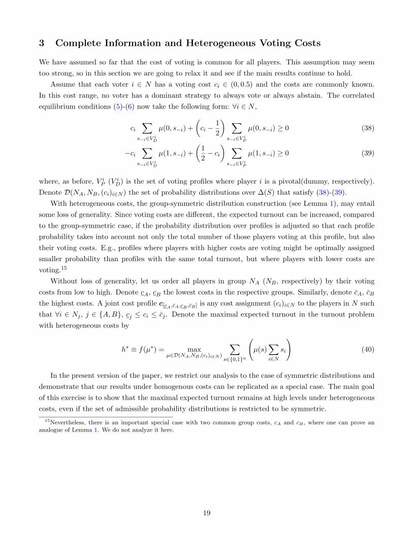
We have assumed so far that the cost of voting is common for all players. This assumption may seem

too strong, so in this section we are going to relax it and see if the main results continue to hold.

Assume that each voter i ∈ N has a voting cost ci ∈ (0, 0.5) and the costs are commonly known.

In this cost range, no voter has a dominant strategy to always vote or always abstain. The correlated

equilibrium conditions (5)-(6) now take the following form: ∀i ∈ N ,

ci∑

s−i∈V iD

µ(0, s−i) +

(ci −

1

2

) ∑s−i∈V i

P

µ(0, s−i) ≥ 0 (38)

−ci∑

s−i∈V iD

µ(1, s−i) +

(1

2− ci

) ∑s−i∈V i

P

µ(1, s−i) ≥ 0 (39)

where, as before, V iP (V i

D) is the set of voting profiles where player i is a pivotal(dummy, respectively).

Denote D(NA, NB, (ci)i∈N ) the set of probability distributions over ∆(S) that satisfy (38)-(39).

With heterogeneous costs, the group-symmetric distribution construction (see Lemma 1), may entail

some loss of generality. Since voting costs are different, the expected turnout can be increased, compared

to the group-symmetric case, if the probability distribution over profiles is adjusted so that each profile

probability takes into account not only the total number of those players voting at this profile, but also

their voting costs. E.g., profiles where players with higher costs are voting might be optimally assigned

smaller probability than profiles with the same total turnout, but where players with lower costs are

voting.15

Without loss of generality, let us order all players in group NA (NB, respectively) by their voting

costs from low to high. Denote cA, cB the lowest costs in the respective groups. Similarly, denote cA, cB

the highest costs. A joint cost profile c[cA,cA,cB ,cB ] is any cost assignment (ci)i∈N to the players in N such

that ∀i ∈ Nj , j ∈ {A,B}, cj ≤ ci ≤ cj . Denote the maximal expected turnout in the turnout problem

with heterogeneous costs by

h∗ ≡ f(µ∗) = maxµ∈D(NA,NB ,(ci)i∈N )

∑s∈{0,1}n

(µ(s)

∑i∈N

si

)(40)

In the present version of the paper, we restrict our analysis to the case of symmetric distributions and

demonstrate that our results under homogenous costs can be replicated as a special case. The main goal

of this exercise is to show that the maximal expected turnout remains at high levels under heterogeneous

costs, even if the set of admissible probability distributions is restricted to be symmetric.

15Nevertheless, there is an important special case with two common group costs, cA and cB , where one can prove ananalogue of Lemma 1. We do not analyze it here.

19

3.1 Symmetric distributions

In this subsection, we require the probability distributions to be group-symmetric. Analogously to Lemma

1, define

MH := {µ ∈ D(NA, NB, (ci)i∈N )|

∀i ∈ NA, ∀b ∈ {0, . . . , nB},∀a ∈ {1, . . . , nA − 1} : µ(0i, a, b) = µ(1i, a− 1, b)

∀k ∈ NB, ∀b ∈ {1, . . . , nB − 1},∀a ∈ {0, . . . , nA} : µ(0k, a, b) = µ(1k, a, b− 1)}

In words, MH is the set of group-symmetric probability distributions over joint profiles which are also

correlated equilibria for complete information and heterogeneous costs. Denote the maximal expected

turnout in the turnout problem with heterogeneous costs and group-symmetric distributions by

h∗ := maxµ∈MH

∑s∈{0,1}n

(µ(s)

∑i∈N

si

)(41)

Clearly, h∗ ≥ h∗. We will now show that an analogue of Proposition 1 holds under the condition

cA = cB.

Proposition 7. Suppose 0 < ci < 0.5 for all i ∈ N . Require µ ∈ MH . Then the following expressions

for h∗ provide the optimal value to the objective in the max turnout problem with heterogeneous costs and

group-symmetric distributions if and only if cA = cB = c and

(i) nB > d12nAe, with h∗ = 2nB;

(ii) nB < d12nAe, with

h∗ = nA ×2cAnB(nA − 1) + nB(nA − 1) + nA(1− 2c)

2cA[nA − nB](nA − 1) + nB(nA − 1) + nA(1− 2c)

= nA × ξ(c, cA)

where it is straightforward to notice that ξ(c, cA) is decreasing in both c and cA, and

a) ξ(c, cA) ∈ (0, 1) for all 0 < c ≤ cA < 12 ;

b) ξ(c, ·)→ 2nBnA

as c→ 12 , so h∗ → 2nB;

c) ξ(·, cA)→ 1 as cA → 0, so h∗ → nA.

Furthermore, 2nB < h∗ < nA.

Proof. See A.9.

Proposition 7 is our second main result. It shows that the maximal expected turnout under correlated

equilibria and group-symmetric distributions behaves similarly to the case of a single voting cost, and

essentially depends on two things: the relative sizes of the groups and the bounds of the support of the

cost distribution. The intuition for the result is similar to Proposition 1. Maximizing turnout implies

that constraint (39) for players in NB binds at the optimum. This in turn implies that constraint (38)

for players in NA binds at the optimum. Now the binding constraint (39) for players in NB crucially

depends on cB, because once it holds for the voters with the highest costs in group NB, it automatically

holds for voters in NB with lower costs. On the other hand, the binding constraint (38) for players in

20

NA crucially depends on cA, because once it holds for the voters with the lowest costs in group NA, it

automatically holds for voters in NA with higher costs. The effects of the two constraints cancel each

other out if and only if cA = cB. Once this condition holds, the key difference between case (i) and case

(ii) under symmetric distributions only concerns the behavior of constraint (38) for players in NB and

constraint (39) for players in NA, just like in Proposition 1.

In the proof of Proposition 7 we show that when cA = cB, the equilibrium distribution support is

the same as in Proposition 1, so Corollary 1 holds without change. For the sake of completeness let us

also provide here the expressions for the probability of the largest tie, πnB ,nB . The only change from

Corollary 2 concerns the case of small minority.

Corollary 4. Suppose nA > nB ≥ 1, 0 < ci < 0.5 for all i ∈ N , and cA = cB = c. Assuming symmetric

distributions,

(i) if nB > d12nAe then

πnB ,nB = 2c


πnB ,nB =2

1c

[1 + 1

2cA(nA−1) + nBnA

(1

2cA− 1)]− 1

cA(nA−1)

Proof. See equations (130) and (151) in the proof of Proposition 7 in A.9.

Notice that if c = cA, the expression for case (ii) coincides with its analogue in Corollary 2.

What happens when cA 6= cB? In A.9 we show that if cB < cA, then the maximal expected turnout

exceeds the value of h∗ for both cases of Proposition 7 and for any admissible combination of the other

cost thresholds. At first sight this might look counterintuitive: cB < cA implies that the majority

group find it costlier to vote than the minority group, so they should vote less. However, the higher

voting cost of the majority group also implies that it will be easier to satisfy their IC constraints for

abstention, as well as the minority group IC constraints for voting. Thus in the group-symmetric max

turnout correlated equilibrium, the competitive profiles with higher total turnout will be assigned higher

probabilities, producing higher expected turnout. As cB → 12 , cB → cA, so the maximal expected

turnout converges to h∗ from above. Similarly, when cB > cA, the maximal expected turnout is lower

than the value of h∗ for both cases of Proposition 7. Nevertheless, as min{cA, cB} → 12 , cA → cB, so

the maximal expected turnout converges to h∗ from below. Therefore, the result of Proposition 7 is, in

a sense, a limiting case when the lowest cost threshold increases towards 12 and symmetric distributions

are assumed.

One can also imagine the case where some voters have costs greater than 12 or less than 0. These cases

are not very interesting from the analysis point of view: if voter i has a dominant strategy to abstain due

to ci >12 (violating constraint (39) for any probability distribution that places a positive probability on

profiles with i voting), her presence in the list of players does not affect at all the outcome of the election,

so we can redefine N ≡ N \ {i}. A more elaborate way to handle this problem requires the use of an

asymmetric probability distribution, which would distinguish i from the other players in her group and

assign probability zero to all profiles with i voting. We do not fully analyze this case, but we conjecture

21

that allowing for high-cost voters will not substantially change our results.

If voter i has a dominant strategy to vote due to ci < 0, then simply removing this voter results

in a loss of generality. The case of negative costs requires some special handling, but it is tractable in

our framework. First of all, without additional assumptions about the distribution of such costs across

groups, one can nevertheless argue that, under the veil of ignorance, voters with negative costs are just

as likely to belong to either of the groups, so we would expect their votes to cancel each other out.

Notwithstanding this argument, we would like to consider the case of negative costs for some voters for

the following reasons. First, it suggests a turnout model that incorporates some additional factors, like

citizen duty, which may be important for some voters. Second, we need to consider the negative costs

to be able to directly compare our results with Palfrey and Rosenthal (1985), who in their Assumption

2 explicitly include them. It is important to understand whether we get a high turnout equilibria due

to our solution concept being the correlated equilibrium, or due to a different assumption about the cost

support.

Let L ⊂ N be the set of voters with (strictly) negative costs. We restrict the set of admissible joint

distributions to those that place probability zero on voters in L receiving a recommendation to abstain

and probability one on voters in L receiving a recommendation to vote. With this modification, we can

simply replace the actual group sizes, nA and nB with their modified versions, nA and nB, which take

into account the voters from L so that nA = nA −LA and nB = nB −LB. This is as if the actual group

sizes are shifted by a constant. It is clear that our results hold for the modified game.

4 Incomplete Information

Incomplete information in the voter turnout game was introduced by Ledyard (1981), and further explored

in Palfrey and Rosenthal (1985). Under incomplete information, (Palfrey and Rosenthal (1985, Theorem

2)) established that in the quasi-symmetric Bayesian Nash equilibrium only voters with non-positive

voting costs will vote in the limit as nA, nB get large. There are several ways to introduce the incomplete

information into the basic model, but not all of them are suitable for the analysis of high-turnout correlated

equilibria. In this section we consider the simplest version.

In general, player i’s type is a pair (ti, ci) of her political type (candidate preference) and the corre-

sponding cost of voting. The political type directly affects the utilities of all voters, but the voting cost

type only affects the utility of a specific player. In this section we assume, for simplicity, that voters’ po-

litical types are common knowledge.16 We use t to denote the fixed commonly known joint political type

where each voter i has political type ti. The costs of voting are stochastic: each voter i ∈ N , draws her

private cost of voting, ci, from a commonly known discrete17 distribution Fti with support {cti , . . . , cti},where 0 < cti ≤

12 and 0 < cti < 1. The assumption about the support range helps rule out uninteresting

equilibria, e.g. those with everyone voting for sure, or those with everyone abstaining for sure. We assume

ci is distributed independently of all other voters’ costs c−i (and types t−i). Distributions FA and FB

16This assumption is in line with Palfrey and Rosenthal (1985) and can be relaxed. We impose it primarily for presentationconvenience.

17Typically it is assumed in the literature that the cost distributions are absolutely continuous. We do not make thisassumption to avoid dealing with measurability issues in the definition of a strategic form correlated equilibrium below. SeeCotter (1991) for a detailed discussion of these issues.

22

determine the set of admissible joint cost profiles, characterized by the tuple of respective cost bounds

(cA, cA, cB, cB) as

C(cA,cA,cB ,cB) ≡ {(ci)i∈N |cti ≤ ci ≤ cti} (42)

We write C−i(cA,cA,cB ,cB) to refer to the set of admissible cost profiles for players other than i. Denote π(c)

the probability of a joint cost profile c = ((ci)i∈N ) ∈ C(cA,cA,cB ,cB). Let Ci denote the random variable

that determines player i’s voting cost. The independently distributed costs then imply that

π(c) ≡

∏{i∈N :ti=A}

FA(ci)

∏{i∈N :ti=B}

FB(ci)

Since the political types are fixed by assumption, we omit the respective component in the definition

of players’ strategies and for each i ∈ N define a pure strategy si : {cti , . . . , cti} → {0, 1A, 1B} as a

function that maps voter i’s cost into an action (abstain, vote for candidate A, or vote for candidate B,

respectively). We assume that voters never vote for the candidate of the opposite political type, so we

abuse notation and merge 1A and 1B into 1 meaning the act of voting for the “correct” candidate. The

set of all pure strategies for player i ∈ N is a finite set Si = {0, 1}{cti ,...,cti}, i.e. the set of all functions

from cost types into actions. Let S ≡ ×i∈NSi be the set of all joint strategies.

The utility of player i from a joint strategy s(c) ≡ (sj(cj)j∈N ) when player i’s voting cost is ci (and

the joint political type is t) takes the following form:

ui(s(c)|ci) =

1− si(ci)ci if∑

{j∈N |tj=ti}sj(cj) >

∑{j∈N |tj 6=ti}

sj(cj)

12 − si(ci)ci if

∑{j∈N |tj=ti}

sj(cj) =∑

{j∈N |tj 6=ti}sj(cj)

−si(ci)ci if∑

{j∈N |tj=ti}sj(cj) <

∑{j∈N |tj 6=ti}

sj(cj)

Let us now discuss the solution concept. There are quite a few alternative definitions of the correlated

equilibrium in games with incomplete information (see in particular Forges (1993, 2006, 2009), Section

8.4 of Bergemann and Morris (2013) and Milchtaich (2013)), which are often far from being equivalent.

The sets of expected payoffs corresponding to specific definitions are (sometimes) partially ordered by

inclusion. We use the strategic form incomplete information correlated equilibrium, as defined in Forges

(1993, 2006). This is the strongest definition in the sense that it results in the smallest set of expected

payoffs compared, for example, to the communication equilibrium (Myerson (1986), Forges (1986)). Hence

if we can obtain a substantial turnout in the strategic form correlated equilibrium, then we can also obtain

it in any of the more general definitions of the correlated equilibrium under incomplete information.

A Strategic Form Incomplete Information Correlated Equilibrium(SFIICE) is a probability distribu-

tion q ∈ ∆(S) that selects a pure strategy profile s = (si)i∈N with probability q(s), such that when

recommended si and knowing her type, no player has an incentive to deviate, given that other players

follow their recommendations. Formally, q ∈ ∆(S) is a SFIICE if for all i ∈ N , all ci ∈ {cti , . . . , cti}, all

23

ai ∈ {0, 1}, and any si ∈ Si such that si(ci) = ai, we have

∑{c−i∈C−i

(cA,cA,cB,cB)

}π(c)∑a−i

∑{s−i(c−i)=a−i}

q(si, s−i)

[ui(ai, a−i)− ui(a′i, a−i)] ≥ 0

for all a′i ∈ {0, 1}.It will be convenient to explicitly rewrite these conditions as the set of distributions q ∈ ∆(S) such

that for all i ∈ N , all ci ∈ {cti , . . . , cti}, and all si ∈ Si such that si(ci) = 0 we have

∑c−i

π(c)

ci ∑a−i∈V i

D


q(si, s−i|si(ci) = 0)

+

(ci −

1

2

) ∑a−i∈V i

P



≥ 0 (43)

and for all si ∈ Si such that si(ci) = 1 we have

∑c−i

π(c)

−ci ∑a−i∈V i

D



+

(1

2− ci

) ∑a−i∈V i

P



≥ 0 (44)

where, as before, V iP and V i

D are the set of joint action profiles such that player i is pivotal and dummy, re-

spectively, and the summation over the others’ costs is understood to be over cost profiles in C−i(cA,cA,cB ,cB).

The induced probability distribution over action profiles at every cost profile c ∈ C(cA,cA,cB ,cB) is given by

ν(a|c) ≡∑

{s∈S|∀i∈N :si(ci)=ai}

q(s) (45)

The max turnout problem under incomplete information now takes the following form:

g∗ ≡ maxq∈D(NA,NB ,FA,FB)

∑{c∈C(cA,cA,cB,cB)}

π(c)

∑a∈{0,1}n

ν(a|c)

(∑i∈N

ai

) (46)

Full characterization of the solution to this problem is not our goal in this section. Rather, we just

want to show a possibility result, that correlated equilibria with substantial turnout can survive in the

incomplete information case. The next proposition delivers the desired result.

Proposition 8. Suppose nA, nB ≥ 1 and nA > nB. Let FA, FB be any discrete distributions over players’

voting costs, {cA, . . . , cA}, and {cB, . . . , cB}, respectively, such that cB ≤ cA ∈ (0, 0.5), 0 < cA < 0.5, and

0 < cB < 0.5. Then g∗ ≥ h∗, where h∗ is defined in (41).

Proof. See A.10.

24

It is straightforward to see that this result holds for large electorates as well.18

Concluding this section, we consider another extension of the basic model, which has incomplete infor-

mation about the relative party sizes. We will assume that N, |N | = n is known, but there is uncertainty

about nA and nB, captured by a commonly known probability distribution PN ∈ ∆({1, . . . , n− 1}), with

PN (m) = Prob(nA = m) for m ∈ {1, . . . , n− 1}.19 Obviously, Prob(nB = m) = Prob(nA = n−m). For

simplicity, we will maintain the assumption of the common voting cost c ∈ (0, 0.5). The next proposition

shows that the high-turnout correlated equilibria remain a benchmark case in this setting.

Proposition 9. Suppose nA is distributed with distribution function PN , defined above, and 0 < c < 0.5.

Then the maximal expected turnout supported in SFIICE is at least EPN(f∗), with expectation taken with

respect to PN and f∗(m) defined in Proposition 1 for each m ∈ {1, . . . , n− 1}.

Proof. See A.11.

5 Discussion

Since Nash equilibria are also correlated equilibria, it is important to understand what exactly the analysis

of correlated equilibria adds to the existing results in the literature.

Under complete information and common voting cost, our paper extends Palfrey and Rosenthal (1983),

who characterized two classes of the Nash equilibria that exhibit substantial turnout and survive when the

electorate becomes large.20 Palfrey and Rosenthal call those mixed-pure strategy equilibria and symmetric

totally-mixed strategy equilibria, respectively. The former equilibria require all voters in one group mixing

between voting and abstention with some common probability, whereas voters in the other group are

further divided into two subgroups such that all voters in one subgroup vote for sure, and all voters in

the other subgroup abstain for sure. The latter equilibria require voters in each group mixing with the

same group-specific probability. Both of these equilibrium classes have a counter-intuitive property: the

expected turnout is increasing in cost. Furthermore, symmetric totally-mixed equilibria only exist when

the cost is large enough and both groups have the same size. This unfortunate dependence on both

groups having exactly the same size translates directly into the incomplete information case, and, in a

sense, is the primary reason why no high-turnout equilibria survive even slightest uncertainty in Palfrey

and Rosenthal (1985) when the electorate size gets large. The corresponding result in this paper (see

Proposition 1) has neither of these shortcomings.

Under heterogeneous voting costs, we can compare our Proposition 7 with Taylor and Yildirim (2010,

Proposition 2). They find that under incomplete information, in large electorates the limit expected

turnout and the probability of winning are completely determined by the lowest voting costs in each group.

In contrast, the max turnout correlated equilibrium puts a joint restriction both on the lowest voting

cost in one group and the highest voting cost in the other. This is the effect of two opposing incentive

compatibility constraints. In a quasi-symmetric Bayesian Nash equilibrium in cutpoint strategies, which

18In particular, we mean the case where the ratio between group sizes remains fixed as their sizes increase to ∞, withfixed cost supports.

19We assume that for any split into two groups, there is always at least one person supporting the other candidate.20This latter criterion is important: Palfrey and Rosenthal (1983) identify many other equilibria that have nice properties,

but do not survive in large electorates.

25

is typically considered in the literature, the two constraints for each group merge into one at the critical

cost. Another related result is Kalandrakis (2007), who proves that under complete information and

heterogeneous costs almost all Nash equilibria are regular, and there exists at least one monotone Nash

equilibrium, where players with higher costs participate with weakly lower probabilities. In our group-

symmetric max-turnout correlated equilibria a similar logic allows to restrict attention to the lowest and

highest costs in each group.

Under incomplete information, we extend Palfrey and Rosenthal (1985). Their high-turnout equilibria

do not survive even slightest uncertainty when the electorate size gets large. In contrast, our high-

turnout correlated equilibria persist (see Propositions 8 and 9). This result can be also compared with

Kalandrakis (2009), who basically shows that high turnout Nash equilibria of the complete information

game with a common positive cost can persist under incomplete information. Assuming that densities of

the private voting cost, private benefit, or both, converge to a point mass that corresponds to a complete

information turnout game with a positive common voting cost, Kalandrakis (2009, Thm 4) permits

introducing incomplete information with respect to individual voting cost, the size of each candidate’s

support, or both. The crucial difference from Palfrey and Rosenthal (1985)’s negative result on high-

turnout equilibria under incomplete information is that Kalandrakis holds the size of the electorate fixed,

and varies the uncertainty level, while Palfrey and Rosenthal hold the uncertainty level fixed and vary

the total size of the electorate. A natural restriction on Kalandrakis’ results comes from the fact that

the Nash equilibria of the complete information game can be approximated by Bayesian equilibria only

for sufficiently small perturbations. Thus while Kalandrakis (2009) established regularity of the class of

asymmetric Nash equilibria which was typically dismissed in the literature due to lack of tractability, he

does not resolve the turnout paradox. Our results, in a sense, provide a link between those two papers.

We show in Proposition 8 that group-symmetric max-turnout correlated equilibria can be preserved under

incomplete information about voting costs, while correlation allows to maintain high-turnout for large

electorates, as long as cost supports are fixed. In Proposition 9 we also show that group-symmetric

max-turnout correlated equilibria can be preserved under incomplete information about relative party

sizes.

One potential criticism of our model concerns the idea of maximizing the expected total turnout

without separate considerations for turnout in each group of supporters. It is not clear a priori whether

the our model can be consistent with the models of the group-based ethical voter approach (e.g., Shachar

and Nalebuff (1999), Feddersen and Sandroni (2006), Coate and Conlin (2004)), if we assume that both

groups independently maximize the turnout among their own members. It is easy to see, however, that

our results in Proposition 1 show that when the minority is large, the same level of maximal expected

total turnout can be achieved when groups maximize their members’ turnout independently. We relegate

more general analysis to a companion paper (Pogorelskiy (2014)), which explicitly addresses coordination

among groups in a new equilibrium concept.

6 Concluding remarks

This is the first paper to introduce and characterize the set of correlated equilibria in the voter turnout

games. The solution concept of the correlated equilibrium, developed by Aumann (1974, 1987), allows us

26

to explicitly take into account the possibilities of pre-play communication between voters. Communication

expands the set of equilibrium outcomes in turnout games thereby providing a micro foundation for group-

based mobilization, as well as a solution to the turnout paradox that does not require ad hoc assumptions

about voters’ utility.

We analyzed the correlated equilibrium turnout in three main settings, varying the information struc-

ture (complete and incomplete) and the assumptions on agents’ voting costs (homogenous and heteroge-

neous).

Under complete information and homogenous voting cost, we fully characterized the turnout bounds

in terms of the correlated equilibria that maximize and minimize the expected turnout. These bounds

provide a theoretical constraint on the levels of turnout that can be achieved if there are no restrictions

on pre-play communication, and also characterize the range of expected turnout implementable in a

correlated equilibrium. The set of correlated equilibria includes all equilibria arising under any of the

more restricted communication protocols, e.g. voter communication in networks.

We found that there are two classes of the max turnout correlated equilibria, determined by the

relative sizes of the two competing groups. If the minority is at least half the size of the majority, the

resulting expected turnout is twice the size of the minority and does not depend on the cost. If the

minority is less than half the size of the majority, the resulting expected turnout is a decreasing function

of the voting cost that starts at the size of the majority for low costs and goes down to twice the size of

the minority for high costs. We also characterized the equilibrium distribution support and several key

election statistics (probabilities of a tie and of the majority winning). In contrast to the high-turnout

Nash equilibria, the high-turnout correlated equilibria possess intuitive properties. For example, the

majority group is more likely to win for all costs, and the tie probability is increasing in the cost. We also

characterize the correlated equilibria that maximize social welfare. Those are generally different from the

minimal turnout equilibria, but exhibit a similar range of expected turnout.

We then showed that the high-turnout equilibria under complete information and homogenous voting

cost have analogues under heterogenous costs, which also remain feasible correlated equilibria under

incomplete information about voting costs. Furthermore, the high-turnout equilibria can be constructed

under incomplete information about relative party sizes.

Our results emphasize the important role of communication in turnout games. A natural question

remains: why is the correlated equilibrium a reasonable solution concept? How, exactly, the correlated

equilibria we describe in this paper can be implemented? The answer to the first question is given

by Aumann (1987) and Hart and Mas-Colell (2000). Correlated equilibrium can be interpreted as an

“expression of Bayesian rationality”: if it is common knowledge that every player maximizes expected

utility given her (subjective) beliefs about the state of the world, the resulting strategy choices form

a correlated equilibrium. Furthermore, correlated equilibrium can be obtained as a result of a simple

dynamic procedure driven by players’ regret over past period observations.

The answer to the second question typically invokes describing a direct mechanism where an impartial

mediator, such as a leader, gives recommendations to players. However it is important to realize that

a correlated equilibrium can be also implemented without the mediator, as a Nash (or even sequential)

equilibrium of the expanded game with simple communication.21 Laboratory experiments are a useful tool

21See Forges (1990), Gerardi (2004), and Gerardi and Myerson (2007).

27

for understanding the effects of unmediated communication on turnout in a controlled setting. Elsewhere

(Palfrey and Pogorelskiy, 2014) we show that these effects are nuanced: with a low voting cost, party-

restricted communication increases turnout, while public communication decreases turnout; while with a

high voting cost, public communication increases turnout. From a theoretical perspective, establishing a

realistic communication scheme that is “minimally necessary” for implementing high-turnout correlated

equilibria remains a promising extension that we leave for future research.

References

Agranov, M, Goeree, J, Romero, J and Yariv, L 2013, ‘What Makes Voters Turn Out: The Effects of

Polls and Beliefs’. Mimeo, Caltech.

Ali, S N, and Lin, C 2013, ‘Why People Vote: Ethical Motives and Social Incentives’, AEJ: Microeco-

nomics, 5(2):73–98.

Aumann R 1974, ‘Subjectivity and Correlation in Randomized Strategies’, Journal of Mathematical

Economics, vol. 1, pp. 67–96.

Aumann R 1987, ‘Correlated Equilibrium as an Expression of Bayesian Rationality’, Econometrica,

vol. 55, pp. 1–18.

Barber, M and Imai, K 2014, ‘Estimating neighborhood effects on turnout from geocoded voter registra-

tion records’. Mimeo, Princeton.

Barelli, P and Duggan, J 2013,‘Purification of Bayes Nash equilibrium with correlated types and inter-

dependent payoffs’. Mimeo, University of Rochester.

Bartels, L M 1996, ‘Uninformed votes: information effects in presidential elections’, American Journal of

Political Science, vol. 40, no. 1, pp.194–230.

Becker, G S 1983,‘A theory of competition among pressure groups for political influence’, Quarterly

Journal of Economics, 98:371–400.

Bendor, J, Diermeier, D, Siegel, D, and Ting, M, ‘A Behavioral Theory of Elections’, Princeton University

Press, 2011.

Bergemann, D and Morris, S 2013, ‘Bayes Correlated Equilibrium and the Comparison of Information

Structures’. Mimeo, Yale University.

Bond, RM, Fariss, CJ, Jones, JJ, Kramer, ADI, Marlow, C, Settle, JE, and Fowler, J H, 2012, ‘A

61-million-person experiment in social influence and political mobilization’, Nature, 489: 295-298.

Borgers, T 2004, ‘Costly voting’, American Economic Revivew, vol. 94, no. 1, pp. 57-66.

Campbell, J 1999, ‘Large electorates and decisive minorities’, Journal of Political Economy, vol. 107,

no. 6, pp. 1199-1217.

28

Cavaliere, A 2001, ‘Coordination and provision of discrete public goods by correlated equilibria’, Journal

of Public Economic Theory, vol. 3, no. 3, pp. 235–255.

Coate, S and Conlin, M 2004, ‘A Group Rule-Utilitarian Approach to Voter Turnout: Theory and

Evidence’, American Economic Review, vol. 94, no. 5, pp. 1476–1504.

Cotter, K 1991, ‘Correlated equilibrium in games with type-dependent strategies’, Journal of Economic

Theory, vol. 54, pp. 48–68.

Cox, G W 1999, ‘Electoral Rules and the Calculus of Mobilization’, Legislative Studies Quarterly, vol. 24,

no. 3, pp. 387–419

DellaVigna, S, List, JA, Malmendier, U, and Rao, G 2014, ‘Voting to Tell Others’, NBER Working paper

no. 19832

Diermeier, D and Van Mieghem, J A 2008, ‘Coordination and turnout in large elections’, Mathematical

and Computer Modelling, vol. 48, pp. 1478–1496.

Downs, A. ‘An Economic Theory of Democracy’, Harper and Row: New York, 1957.

Evren, O 2012, ‘Altruism and Voting: A Large-Turnout Result That Does not Rely on Civic Duty or

Cooperative Behavior’, Journal of Economic Theory, 147(6):2124–2157.

Feddersen, T 2004 ‘Rational choice theory and the paradox of not voting’, Journal of Economic Perspec-

tives, vol. 18, no. 1, pp. 99-112.

Feddersen, T J and Sandroni, A 2006 ‘A Theory of Participation in Elections’, American Economic

Review, vol. 94, no. 4, pp. 1271–1282

Forges, F 1986, ‘An Approach to Communication Equilibria’, Econometrica, vol. 54, no. 6, pp. 1375–1385.

Forges, F 1990, ‘Universal mechanisms’, Econometrica, vol. 58, pp. 1341–1364.

Forges, F 1993, ‘Five legitimate definitions of correlated equilibrium in games with incomplete informa-

tion’, Theory and Decision, vol. 35, pp. 277–310.

Forges, F 2006, ‘Correlated equilibrium in games with incomplete information revisited’, Theory and

Decision, vol. 61, pp. 329–344.

Forges, F. ‘Correlated equilibria and communication in games’, In: R A Meyers (ed.) ‘Encyclopedia of

Complexity and Systems Science’, Springer: Berlin, 2009.

Gerardi, D 2004, ‘Unmediated communication in games with complete and incomplete information’,

Journal of Economic Theory, 114: 104-131.

Gerardi, D, and Myerson, R B 2007, ‘Sequential equilibria in Bayesian games with communication’,

Games and Economic Behavior, 60: 104-134.

Gerber, A S, and Green, D P 2000, ‘The Effects of Canvassing, Telephone Calls, and Direct Mail on

Voter Turnout: A Field Experiment’, American Political Science Review, vol. 94, no. 3, pp. 653-63.

29

Gerber, A S, and Green, D P. ‘Get Out the Vote: How to Increase Voter Turnout’. Brookings Institution

Press, 2008.

Gerber, A S, Green, D P, and Larimer, C W 2008, ‘Social pressure and voter turnout: evidence from a

large-scale field experiment’, American Political Science Review, vol. 102, no. 1, pp. 33-48.

Gerber, A S, Gimpel, J G, Green, D P, and Shaw, D R, 2011, ‘How Large and Long-lasting Are the Per-

suasive Effects of Televised Campaign Ads? Results from a Randomized Field Experiment’, American

Political Science Review, vol. 105, no. 1, pp. 135-150.

Geys, B 2006 ‘”Rational” Theories of Voter Turnout: A Review’, Political Studies Review, 4(1), 16-35.

Goeree, J K and Grosser, J 2007, ‘Welfare reducing polls’, Economic Theory, vol. 31, pp. 51-68.

Goeree, J K and Yariv, L 2011, ‘An Experimental Study of Collective Deliberation’, Econometrica, vol. 79,

no. 3, pp. 893-921.

Gomez, B, Hansford, T G, and Krause, G A 2007, ‘The Republicans Should Pray for Rain: Weather,

Turnout, and Voting in U.S. Presidential Elections’, Journal of Politics, vol. 69, pp. 649-663.

Grosser, J K and Schram, A 2006, ‘Neighborhood Information Exchange and Voter Participation: An

Experimental Study’, American Political Science Review, vol. 100, no. 2, pp. 235–48.

Grosser, J and Schram, A 2010, ‘Public Opinion Polls, Voter Turnout, and Welfare: An Experimental

Study’, American Journal of Political Science, vol. 54, no. 3, pp. 700-717.

Hart, S and Mas-Colell A 2000, ‘A Simple Adaptive Procedure Leading to Correlated Equilibrium’,

Econometrica, vol. 68, no. 5, pp. 1127-1150.

Kalandrakis, T 2007, ‘On participation games with complete information’, International Journal of Game

Theory, 35: 337–352.

Kalandrakis, T 2009, ‘Robust rational turnout’, Economic Theory, vol. 41, no. 2, pp. 317–343.

Krasa, S, Polborn, M 2009, ‘Is mandatory voting better than voluntary voting?’, Games and Economic

Behavior, vol. 66, no. 1, pp. 275-291.

Lassen, D D 2005, ‘The Effect of Information on Voter Turnout: Evidence from a Natural Field Experi-

ment’, American Journal of Political Science, vol. 49, no. 1, pp. 103-18.

Ledyard, J, ‘The paradox of voting and candidate competition: a general equilibrium analysis’. In: G

Horwich and J Quirk (eds.) ‘Essays in contemporary fields of economics’. West Lafayette, Ind.: Purdue

University Press, 1981.

Ledyard, J 1984 ‘The pure theory of large two-candidate elections’, Public Choice, vol. 44, no. 1, pp. 7-41.

Levine, D and Palfrey, T R 2007, ‘The paradox of voter participation? A laboratory study’, American

Political Science Review, vol. 101, no. 1, pp. 143–158.

30

McMurray, J 2012, ‘The paradox of information and voter turnout’, Mimeo, Brigham Young University.

McMurray, J 2013, ‘Aggregating information by voting: the wisdom of the experts versus the wisdom of

the masses’, Review of Economic Studies, vol. 80, pp. 277–312.

Merlo, A and Palfrey, T R 2013, ‘External validation of voter turnout models by concealed parameter

recovery’, Social Science Working Paper 1370, California Institute of Technology.

Milchtaich, I 2013, ‘Implementability of Correlated and Communication Equilibrium Outcomes in In-

complete Information Games’, International Journal of Game Theory, pp.1–68. DOI: 10.1007/s00182-

013-0381-y

Morton, R 1991, ‘Groups in Rational Turnout Models’, American Journal of Political Science, vol. 35,

no. 3, pp. 758–776.

Myatt D P 2012, ‘A Rational Choice Theory of Voter Turnout’. Mimeo, London Business School.

Myerson, R B 1982, ‘Optimal coordination mechanisms in generalized principal-agent problems’, Journal

of Mathematical Economics, vol. 10, pp. 67–81.

Myerson, R B 1986, ‘Multistage Games with Communication’, Econometrica, vol. 54, no. 2, pp. 323–358.

Myerson, R B 1991, ‘Game theory: analysis of conflict’. Cambridge, MA: Harvard University Press.

Myerson, R B 1998, ‘Population uncertainty and Poisson games’, International Journal of Game Theory,

vol. 27, pp. 375–392.

Myerson, R B 2000, ‘Large Poisson Games’, Journal of Economic Theory, vol. 94, pp. 7–45.

Ortoleva, P, and Snowberg, E, 2014,‘Overconfidence in Political Behavior’, American Economic Review,

forthcoming.

Palfrey, T R 2013 ‘Experiments in Political Economy’, In: J Kagel and A Roth (eds.) Handbook of

Experimental Economics, Vol. 2, forthcoming.

Palfrey, T R and Pogorelskiy, K 2014, ‘Voter Turnout Games with Communication: An Experimental

Study’, Mimeo, Caltech.

Palfrey, T R and Rosenthal, H 1983 ‘A strategic calculus of voting’, Public Choice, vol. 41, pp. 7–53.

Palfrey, T R and Rosenthal, H 1984 ‘Participation and the provision of discrete public goods: A strategic

analysis’, Journal of Public Economics, vol. 24, pp. 171-193

Palfrey, T R and Rosenthal, H 1985 ‘Voter Participation and Strategic Uncertainty’, American Political

Science Review, vol. 79, pp. 62–78.

Pogorelskiy, K 2014, ‘Subcorrelated and Subcommunication Equilibria’, Mimeo, Caltech.

Riker, W and Ordeshook, P 1968 ‘A Theory of the Calculus of Voting’, American Political Science Review,

vol. 62, pp. 25–42.

31

http://dx.doi.org/10.1007/s00182-013-0381-y

http://dx.doi.org/10.1007/s00182-013-0381-y

Rolfe, M. Voter Turnout: A Social Theory of Political Participation. Cambridge University Press, 2012.

Rosenstone, S J, and Hansen J M. Mobilization, Participation, and Democracy in America. New York:

Macmillan, 1993.

Sanders, M S 2001, ‘Uncertainty and Turnout’, Political Analysis, 9:1, 45–57.

Schram, A, ‘Voter Behavior in Economics Perspective’. Springer Verlag: Heidelberg, 1991.

Schram, A, and Sonnemans, J 1996, ‘Why people vote: Experimental evidence’,Journal of Economic

Psychology, vol. 17, no. 4, pp. 417–442.

Sinclair, B 2012. The Social Citizen: Peer Networks and Political Behavior. University of Chicago Press.

Schram, A, and van Winden, F 1991, ‘Why people vote: Free riding and the production and consumption

of social pressure’, Journal of Economic Psychology, vol. 12, pp. 575–620.

Shachar, R and Nalebuff, B 1999, ‘Follow the Leader: Theory and Evidence on Political Participation’,

American Economic Review, vol. 89, no. 3, pp. 525–547.

Taylor, C R and Yildirim, H 2010 ‘A unified analysis of rational voting with private values and group-

specific costs’, Games and Economic Behavior, no. 70, pp. 457–71.

Tullock, G. Toward a Mathematics of Politics. Ann Arbor: University of Michigan Press, 1967.

Uhlaner, C J 1989, ‘Rational Turnout: The Neglected Role of Groups’, American Journal of Political

Science, vol. 33, no. 2, pp. 390–422.

32

Appendix

A Proofs

A.1 Proof of Lemma 1

Proof. Fix any i ∈ NA and consider two voting profiles: x1 := (0i, a, b) and x2 := (1i, a − 1, b) such

that the total number of votes in group NA is a, the total number of votes in group NB is b, and in

the first profile voter i abstains, while in the second profile i turns out to vote and somebody else from

NA abstains. We will construct the equivalent symmetric distribution iteratively. At step 1, we let

σ∗1(s) = µ∗(s) for all profiles s 6= x1, x2. The objective in either (9) or (10) does not depend on voters’

identities, only on the total number of votes in each profile. Since the total number of votes at either x1

or x2 is the same and equals a+ b, it does not matter for the objective how σ∗1 distributes the probability

mass among x1 and x2 compared to µ∗ as long as µ∗(x1) + µ∗(x2) = σ∗1(x1) + σ∗1(x2). Hence we can let

σ∗1(x1) = σ∗1(x2) = 12(µ∗(x1) + µ∗(x2)). Clearly, this argument holds for any a ∈ {1, . . . , nA − 1}, any

b ∈ {0, . . . , nB}, and any i ∈ NA, and a similar argument holds for any k ∈ NB and profiles (0k, a, b) and

(1k, a, b − 1), respectively. We can now iteratively construct σ∗, where at each step t ≥ 2 we define xt1and xt2 by one of the remaining combinations of (a, b, i), and let σ∗t (s) = σ∗t−1(s) for all profiles s 6= xt1, x

t2.

Once we have considered all combinations, we obtain σ∗, for which by construction f(σ∗) = f(µ∗) and

σ∗ ∈ M. It remains to show that all IC constraints are satisfied at σ∗. To see this, let’s roll back to σ∗1and show that the IC constraints are satisfied at each iteration. Notice that the sets V i

D and V iP in (8)

and (7) do not depend on other voters’ identities, but only on the total number of votes on each side

of the profile, hence x1 ∈ V iP if and only if x2 ∈ V `

P for any ` ∈ NA, ` 6= i such that ` votes at x1 and

abstains at x2 (since a ∈ {1, . . . , nA− 1}, there must exist at least one such player). Similarly, x2 ∈ V iP if

and only if x1 ∈ V `P for any such `. These relations hold for all (x1, x2) with a ∈ {1, . . . , nA− 1}, and any

b ∈ {0, . . . , nB}. By assumption, IC constraints (5)-(6) hold for all i ∈ N under µ∗. Since the voting cost

is the same for everyone in NA, and µ∗ is optimal, the corresponding IC constraints must be of the same

kind (slack or binding) for both i and ` under µ∗, and, moreover, they must put the same restriction on

the total probability that i is pivotal at x1 as they put on the total probability that ` is pivotal at x2, i.e.∑s−i∈V i

P|s−i|=a+b

µ∗(0i, 1`, s−i∪`) =∑

s−`∈V `P

|s−`|=a+b

µ∗(0`, 1i, s−i∪`)

and ∑s−i∈V i

P|s−i|=a−1+b

µ∗(1i, 0`, s−i∪`) =∑

s−`∈V `P

|s−`|=a−1+b

µ∗(1`, 0i, s−i∪`)

But then redistributing this probability mass symmetrically under σ∗ does not violate the IC for i ∈ NA,

a ∈ {1, . . . , nA − 1}, and any b ∈ {0, . . . , nB}. Similarly, we can prove that this redistribution does not

violate the IC for k ∈ NB and b ∈ {1, . . . , nB − 1}, a ∈ {0, . . . , nA}.

33

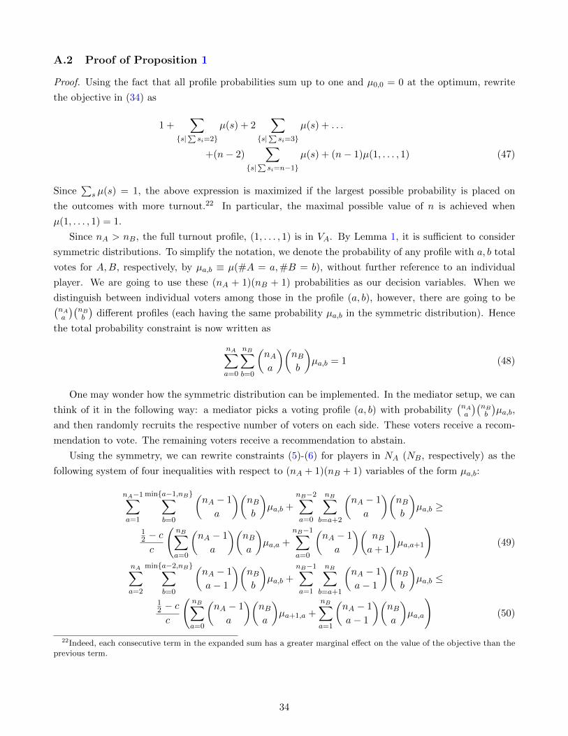
A.2 Proof of Proposition 1

Proof. Using the fact that all profile probabilities sum up to one and µ0,0 = 0 at the optimum, rewrite

the objective in (34) as

1 +∑

{s|∑si=2}

µ(s) + 2∑

{s|∑si=3}

µ(s) + . . .

+(n− 2)∑

{s|∑si=n−1}

µ(s) + (n− 1)µ(1, . . . , 1) (47)

Since∑

s µ(s) = 1, the above expression is maximized if the largest possible probability is placed on

the outcomes with more turnout.22 In particular, the maximal possible value of n is achieved when

µ(1, . . . , 1) = 1.

Since nA > nB, the full turnout profile, (1, . . . , 1) is in VA. By Lemma 1, it is sufficient to consider

symmetric distributions. To simplify the notation, we denote the probability of any profile with a, b total

votes for A,B, respectively, by µa,b ≡ µ(#A = a,#B = b), without further reference to an individual

player. We are going to use these (nA + 1)(nB + 1) probabilities as our decision variables. When we

distinguish between individual voters among those in the profile (a, b), however, there are going to be(nAa

)(nBb

)different profiles (each having the same probability µa,b in the symmetric distribution). Hence

the total probability constraint is now written as

nA∑a=0

nB∑b=0

(nAa

)(nBb

)µa,b = 1 (48)

One may wonder how the symmetric distribution can be implemented. In the mediator setup, we can

think of it in the following way: a mediator picks a voting profile (a, b) with probability(nAa

)(nBb

)µa,b,

and then randomly recruits the respective number of voters on each side. These voters receive a recom-

mendation to vote. The remaining voters receive a recommendation to abstain.

Using the symmetry, we can rewrite constraints (5)-(6) for players in NA (NB, respectively) as the

following system of four inequalities with respect to (nA + 1)(nB + 1) variables of the form µa,b:

nA−1∑a=1

min{a−1,nB}∑b=0

(nA − 1

a

)(nBb

)µa,b +

nB−2∑a=0

nB∑b=a+2

(nA − 1

a

)(nBb

)µa,b ≥

12 − cc

(nB∑a=0

(nA − 1

a

)(nBa

)µa,a +

nB−1∑a=0

(nA − 1

a

)(nBa+ 1

)µa,a+1

)(49)

nA∑a=2

min{a−2,nB}∑b=0

(nA − 1

a− 1

)(nBb

)µa,b +

nB−1∑a=1

nB∑b=a+1

(nA − 1

a− 1

)(nBb

)µa,b ≤

12 − cc

(nB∑a=0

(nA − 1

a

)(nBa

)µa+1,a +

nB∑a=1

(nA − 1

a− 1

)(nBa

)µa,a

)(50)

22Indeed, each consecutive term in the expanded sum has a greater marginal effect on the value of the objective than theprevious term.

34

and

nA∑a=2

min{a−2,nB−1}∑b=0

(nAa

)(nB − 1

b

)µa,b +

nB−2∑a=0

nB−1∑b=a+1

(nAa

)(nB − 1

b

)µa,b ≥

12 − cc

(nB−1∑a=0

(nAa

)(nB − 1

a

)µa,a +

nB−1∑a=0

(nAa+ 1

)(nB − 1

a

)µa+1,a

)(51)

nA∑a=2

min{a−1,nB}∑b=1

(nAa

)(nB − 1

b− 1

)µa,b +

nB−2∑a=0

nB∑b=a+2

(nAa

)(nB − 1

b− 1

)µa,b ≤

12 − cc

(nB−1∑a=0

(nAa

)(nB − 1

a

)µa,a+1 +

nB∑a=1

(nAa

)(nB − 1

a− 1

)µa,a

)(52)

We will refer to the first and the third inequality above as the odd incentive compatibility (IC) constraints,

and to the second and the fourth inequality as the even IC constraints, distinguished by the group.

Since we assumed nA > nB, at the largest turnout profile µ(1, . . . , 1) ≡ µnA,nB voters from NB (as

well as voters from NA, if nA > nB + 1) are dummies. This implies that the even IC constraint for

NB is always binding at the optimum. As for the even IC constraint for NA, we can show that for

nA > nB ≥ d12nAe it is always slack. To see this, notice that the even IC for NA requires

µnA,nB≤

12 − cc

(nB−1∑a=0

(nA − 1

a

)(nBa

)µa+1,a +

nB∑a=1

(nA − 1

a− 1

)(nBa

)µa,a

)

−

[nB−1∑b=1

(nBb

)µnA,b +

nB∑a=3

a−2∑b=1

(nA − 1

a− 1

)(nBb

)µa,b

+

nA−1∑a=nB+2

nB∑b=1

(nA − 1

a− 1

)(nBb

)µa,b +

nB−2∑a=1

nB∑b=a+2

(nA − 1

a− 1

)(nBb

)µa,b

]

−nB−1∑a=1

(nA − 1

a− 1

)(nBa+ 1

)µa,a+1 −

nB∑b=1

(nA − 1

nB

)(nBb

)µnB+1,b −

nB∑a=2

(nA − 1

a− 1

)µa,0

+1

2c

(nA − 1

nB

)µnB+1,nB

−nA∑

a=nB+1

(nA − 1

a− 1

)µa,0 (53)

The binding even IC for NB requires

µnA,nB=

12 − cc

(nB−1∑a=0

(nAa

)(nB − 1

a

)µa,a+1 +

nB∑a=1

(nAa

)(nB − 1

a− 1

)µa,a

)

−

[nB−1∑b=1

(nB − 1

b− 1

)µnA,b +

nB∑a=3

a−2∑b=1

(nAa

)(nB − 1

b− 1

)µa,b

+

nA−1∑a=nB+2

nB∑b=1

(nAa

)(nB − 1

b− 1

)µa,b +

nB−2∑a=1

nB∑b=a+2

(nAa

)(nB − 1

b− 1

)µa,b

]

−nB−1∑a=1

(nAa+ 1

)(nB − 1

a− 1

)µa+1,a −

nB∑b=1

(nA

nB + 1

)(nB − 1

b− 1

)µnB+1,b

−nB∑b=2

(nB − 1

b− 1

)µ0,b (54)

Comparing the right hand sides of these two expressions, we see that in every single term of (53),

35

except for the two terms on the last line, the total profile turnout matches exactly the total profile turnout

in the corresponding term of (54). There are three possibilities. If the RHS of (54) is strictly less than

the RHS of (53), the even IC for NA is slack, so we are done. The RHS of (54) cannot be strictly

greater, since then the even IC for NA does not hold at all, and so we are not at the optimum of the

constrained maximization program. The critical case is when the two RHS are the same; but this holds

at the optimum if and only if the sum of the last two terms of (53) is zero (otherwise, since the profiles in

the last two terms of (53) are not matched in (54), and so are not restricted by (54), the RHS of (53) in

the optimum can be increased without increasing the RHS of (54), which is optimal when nB ≥ d12nAe).

As long as nB ≥ d12nAe, we have 2nB ≥ nA and 2nB + 1 > nA, so

1

2c

(nA − 1

nB

)µnB+1,nB −

nA∑a=nB+1

(nA − 1

a− 1

)µa,0 > 0

That is, the sum of the two terms on the last line of (53) is strictly positive at the optimum. This follows,

since the total turnout of the first term, 2nB + 1, exceeds the total turnout of the largest term in the

above sum, which is nA, achieved at µnA,0. Therefore, the RHS of (54) is strictly less at the optimum

than the RHS of (53) and so the even IC for NA is slack, given that the even IC for NB is binding. Now,

if nB < d12nAe, then 2nB + 1 ≤ nA, so it is easy to see that the even IC constraints for both groups are

binding at the optimum.

As for the odd IC constraints, we can show that the situation is the opposite: the odd IC for NA is

always binding at the optimum, while the odd IC for NB only binds when nB > d12nAe (for even nA)

or nB ≥ d12nAe (for odd nA). To see this, notice that in the binding constraint (54) all profiles such

that a non-voter from NA is a dummy have the negative sign, so we want to reduce them as much as

possible in the optimum. The only subset of profiles where a non-voter from NA is a dummy which is

not directly restricted by (54) has the form∑nA−1

a=1

(nA−1a−1

)µa,0. But these profiles are restricted by (53).

If the latter is binding, the restriction is trivial. Suppose not, then if we reduced all directly restricted by

(54) probabilities to their lower limit of zero and the odd IC for NA still was not binding, then constraint

(53) (slack by assumption) would imply that µnA,nB < 0. Therefore, the odd IC for NA must bind at the

optimum.

Let us now turn to the odd IC constraint for NB. The odd IC for NA is binding as we just demon-

strated, so we can rewrite (49) and (51), respectively, as

nA−1∑a=nB+1

(nA − 1

a

)µa,nB

−12 − cc

(nA − 1

nB

)µnB ,nB

+

(nA − 1

nB

)(nB

nB − 1

)µnB ,nB−1 +

nB−2∑a=0

(nA − 1

a

)µa,nB

+

nB−2∑a=0

(nA − 1

a+ 1

)(nBa

)µa+1,a +

nB+1∑a=2

a−2∑b=0

(nA − 1

a

)(nBb

)µa,b

+

nA−1∑a=nB+2

nB−1∑b=0

(nA − 1

a

)(nBb

)µa,b +

nB−3∑a=0

nB−1∑b=a+2

(nA − 1

a

)(nBb

)µa,b =

12 − cc

(nB−1∑a=0

(nA − 1

a

)(nBa

)µa,a +

nB−1∑a=0

(nA − 1

a

)(nBa+ 1

)µa,a+1

)(55)

36

and

nB−1∑b=0

(nB − 1

b

)µnA,b

+

nB−2∑a=0

(nAa

)(nB − 1

a+ 1

)µa,a+1 +

nB+1∑a=2

a−2∑b=0

(nAa

)(nB − 1

b

)µa,b

+

nA−1∑a=nB+2

nB−1∑b=0

(nAa

)(nB − 1

b

)µa,b +

nB−3∑a=0

nB−1∑b=a+2

(nAa

)(nB − 1

b

)µa,b ≥

12 − cc

(nB−1∑a=0

(nAa

)(nB − 1

a

)µa,a +

nB−1∑a=0

(nAa+ 1

)(nB − 1

a

)µa+1,a

)(56)

Comparing these two expressions, we see that, except for the terms on the first two lines of (55) and

those on the first line of (56), in every remaining profile of (55) the total turnout matches exactly the

total turnout in the corresponding term of (56).

Suppose nB < d12nAe, then 2nB < nA. We want to show that at the optimum

nB−1∑b=0

(nB − 1

b

)µnA,b +

1

2c

(nA − 1

nB

)µnB ,nB >

nA−1∑a=nB+1

(nA − 1

a

)µa,nB +

(nA − 1

nB

)µnB ,nB

+

(nA − 1

nB

)(nB

nB − 1

)µnB ,nB−1 +

nB−2∑a=0

(nA − 1

a

)µa,nB (57)

The case of nA − 1 < nB + 1 is not possible, since then nA = nB + 1, but 2nB < nA implies nB < 1.

So nA − 1 ≥ nB + 1, then nA ≥ nB + 2. Notice that on the RHS of (57) (at profiles with probability

µa,nB in the first sum) the total turnout in each profile equals nB + nA − k, where k ≥ 1, matching the

corresponding turnout in each profile on the LHS of (57) (at profiles with probability µnA,b) as long as

nA−k ≥ nB +1 (since a ≥ nB +1 in the first sum). Once nA−k = nB +1, there are no more profiles left

in the first sum of the RHS of (57), but there remain profiles with probability µnA,b in the corresponding

sum on the LHS of (57) as long as 0 ≤ nB − k ≤ nB − 1, since we have 0 ≤ b ≤ nB − 1. Writing the

largest possible k∗ = nA − nB − 1, we see that since nA ≥ nB + 2 by assumption, we indeed have k∗ ≥ 1.

Therefore, the LHS of (57) contains the profiles with larger turnout that are unmatched by the profiles

on the RHS of (57): at the very least, the corresponding probabilities are µnA,0 and µnA,1. So at the

optimum (57) holds; hence, the odd IC for NB is slack.

Now if nA is even, we can extend this result to the case where nB = d12nAe, since then 2nB = nA, so

even though µnA,1 becomes matched by the first probability in the sum on the RHS, µnB+1,nB , we still

have µnA,0 unmatched on the LHS. However, if nA is odd, then nB = d12nAe implies 2nB = nA + 1, so

µnA,0 becomes matched by µnB ,nB−1, and hence the odd IC for NB is binding at the optimum.

Finally, if nB > d12nAe, then 2nB ≥ nA + 1, so all profiles on the LHS of (57) are matched by the

corresponding profiles on the RHS, so the odd IC for NB is binding.

Table 1 summarizes our findings on binding and slack constraints in the maximization problem. To

finish the proof, we need to consider three cases, corresponding to the columns of Table 1.

37

Table 1: IC constraints at the optimum (max-turnout equilibria)

nB < d 12nAe nB = d 1

2nAe nB > d 12nAe

Odd IC for NA (49) always bindsEven IC for NA (50) binds slack slackOdd IC for NB (51) slack slack for even nA; binds

binds for odd nAEven IC for NB (52) always binds

Note: nA > nB, 0 < c < 12

First, suppose nB > d12nAe. Then the odd IC constraint for NA binding implies

nB+1∑a=1

a−1∑b=0

(nA − 1

a

)(nBb

)µa,b +

nA−1∑a=nB+2

nB∑b=0

(nA − 1

a

)(nBb

)µa,b

+

nB−2∑a=0

nB∑b=a+2

(nA − 1

a

)(nBb

)µa,b −

12 − cc

(nB∑a=0

(nA − 1

a

)(nBa

)µa,a

+

nB−1∑a=0

(nA − 1

a

)(nBa+ 1

)µa,a+1

)= 0, (58)

the odd IC constraint for NB binding implies

nB+1∑a=2

a−2∑b=0

(nAa

)(nB − 1

b

)µa,b +

nA∑a=nB+2

nB−1∑b=0

(nAa

)(nB − 1

b

)µa,b

+

nB−2∑a=0

nB−1∑b=a+1

(nAa

)(nB − 1

b

)µa,b −

12 − cc

(nB−1∑a=0

(nAa

)(nB − 1

a

)µa,a

+

nB−1∑a=0

(nAa+ 1

)(nB − 1

a

)µa+1,a

)= 0, (59)

and the even IC constraint for NB binding implies

µnA,nB=

12 − cc

(nB−1∑a=0

(nAa

)(nB − 1

a

)µa,a+1 +

nB∑a=1

(nAa

)(nB − 1

a− 1

)µa,a

)

−

[nB−1∑b=1

(nB − 1

b− 1

)µnA,b +

nB∑a=2

a−1∑b=1

(nAa

)(nB − 1

b− 1

)µa,b

+

nA−1∑a=nB+1

nB∑b=1

(nAa

)(nB − 1

b− 1

)µa,b +

nB−2∑a=0

nB∑b=a+2

(nAa

)(nB − 1

b− 1

)µa,b

](60)

At the optimum, µnA,nB must be as large as possible. This implies that the terms in the first parentheses

must be as large as possible, and in particular, the last term in the second sum,(nAnB

)µnB ,nB , since it has

38

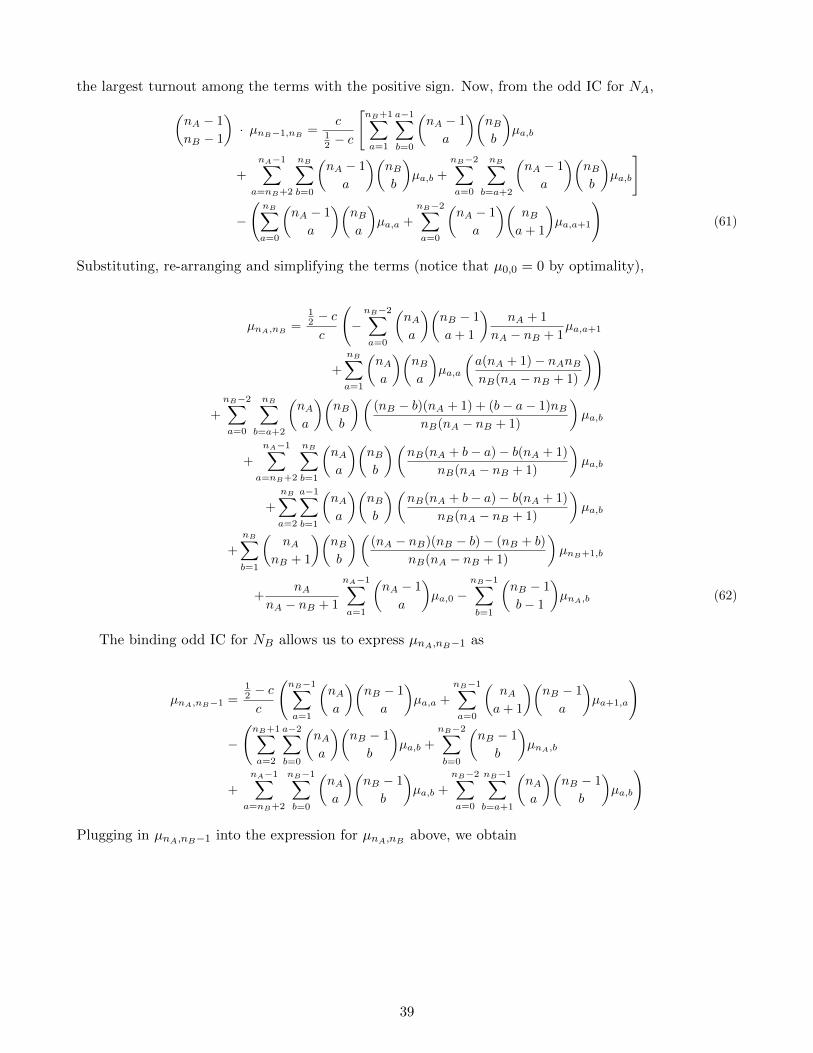
the largest turnout among the terms with the positive sign. Now, from the odd IC for NA,(nA − 1

nB − 1

)· µnB−1,nB

=c

12 − c

[nB+1∑a=1

a−1∑b=0

(nA − 1

a

)(nBb

)µa,b

+

nA−1∑a=nB+2

nB∑b=0

(nA − 1

a

)(nBb

)µa,b +

nB−2∑a=0

nB∑b=a+2

(nA − 1

a

)(nBb

)µa,b

]

−

(nB∑a=0

(nA − 1

a

)(nBa

)µa,a +

nB−2∑a=0

(nA − 1

a

)(nBa+ 1

)µa,a+1

)(61)

Substituting, re-arranging and simplifying the terms (notice that µ0,0 = 0 by optimality),

µnA,nB=

12 − cc

(−

nB−2∑a=0

(nAa

)(nB − 1

a+ 1

)nA + 1

nA − nB + 1µa,a+1

+

nB∑a=1

(nAa

)(nBa

)µa,a

(a(nA + 1)− nAnBnB(nA − nB + 1)

))

+

nB−2∑a=0

nB∑b=a+2

(nAa

)(nBb

)((nB − b)(nA + 1) + (b− a− 1)nB

nB(nA − nB + 1)

)µa,b

+

nA−1∑a=nB+2

nB∑b=1

(nAa

)(nBb

)(nB(nA + b− a)− b(nA + 1)

nB(nA − nB + 1)

)µa,b

+

nB∑a=2

a−1∑b=1

(nAa

)(nBb

)(nB(nA + b− a)− b(nA + 1)

nB(nA − nB + 1)

)µa,b

+

nB∑b=1

(nA

nB + 1

)(nBb

)((nA − nB)(nB − b)− (nB + b)

nB(nA − nB + 1)

)µnB+1,b

+nA

nA − nB + 1

nA−1∑a=1

(nA − 1

a

)µa,0 −

nB−1∑b=1

(nB − 1

b− 1

)µnA,b (62)

The binding odd IC for NB allows us to express µnA,nB−1 as

µnA,nB−1 =12 − cc

(nB−1∑a=1

(nAa

)(nB − 1

a

)µa,a +

nB−1∑a=0

(nAa+ 1

)(nB − 1

a

)µa+1,a

)

−

(nB+1∑a=2

a−2∑b=0

(nAa

)(nB − 1

b

)µa,b +

nB−2∑b=0

(nB − 1

b

)µnA,b

+

nA−1∑a=nB+2

nB−1∑b=0

(nAa

)(nB − 1

b

)µa,b +

nB−2∑a=0

nB−1∑b=a+1

(nAa

)(nB − 1

b

)µa,b

)

Plugging in µnA,nB−1 into the expression for µnA,nB above, we obtain

39

µnA,nB=

12 − cc

1

nA − nB + 1

(nAnB

)µnB ,nB

+

nA−1∑a=nB+1

(nAa

)(nB − a− 1

nA − nB + 1

)µa,nB

+12 − cc

nB−1∑a=1

(nAa

)(nBa

)((a− nB)(2nA − nB + 1) + a

nB(nA − nB + 1)

)µa,a

+(nA + 1)(2− 1

2c )− nBnA − nB + 1

nB−2∑a=0

(nAa

)(nB − 1

a+ 1

)µa,a+1

+

nB−1∑a=1

(nAa+ 1

)(nBa

)(− 12−cc (nB − a)(nA − nB + 1) + nA(nB − a)− (nB + a)

nB(nA − nB + 1)

)µa+1,a

+

(c(nA − 1)−

(12 − c

)(nA − nB + 1)

c(nA − nB + 1)

)nAµ1,0 +

nB−2∑a=0

(nAa

)(nB − a− 1

nA − nB + 1

)µa,nB

+

nB−3∑a=0

nB−1∑b=a+2

(nAa

)(nBb

)((nB − b)(2nA − nB + 1) + (b− a− 1)nB

nB(nA − nB + 1)

)µa,b

+

nA−1∑a=nB+2

nB−1∑b=1

(nAa

)(nBb

)((nB − b)(2nA − nB + 1) + (b− a− 1)nB

nB(nA − nB + 1)

)µa,b

+

nB∑a=3

a−2∑b=1

(nAa

)(nBb

)((nB − b)(2nA − nB + 1) + (b− a− 1)nB

nB(nA − nB + 1)

)µa,b

+

nA−1∑a=2

(nAa

)2nA − nB + 1− anA − nB + 1

µa,0 +

nB−2∑b=0

(nBb

)(nB − 2b

nB

)µnA,b

+

nB−1∑b=1

(nA

nB + 1

)(nBb

)((nB − b)(2nA − 2nB + 1)− (nB + b)

nB(nA − nB + 1)

)µnB+1,b (63)

It is important to determine the signs of all the terms in the above expression. It is easy to see

that the first term (the largest tied profile) is positive, the next one negative. The terms with µa,a, a ∈{1, . . . , nB − 1}, are negative, as well as the terms with µa,a+1, a ∈ {0, . . . , nB − 2}.23 The terms with

µa+1,a, a ∈ {1, . . . , nB − 1}, are negative too.24 The term with µ1,0 can be positive depending on the

cost (but has the lowest possible total turnout). The remaining terms on the same line are positive.

All terms on the next three lines (terms with µa,b for a ∈ {0, . . . , nB − 3}, b ∈ {a + 2, . . . , nB − 1};a ∈ {nB + 2, . . . , nA − 1}, b ∈ {1, . . . , nB − 1}; and a ∈ {3, . . . , nB}, b ∈ {1, . . . , a − 2}) are positive.25

The terms with µa,0, a ∈ {2, . . . , nA − 1} are all positive. The last term on the same line (with µnA,b) is

positive for b ∈ [0, bnB2 c] and negative for b ∈ [bnB

2 c+ 1, nB − 2]. The terms on the last line (terms with

µnB+1,b, b ∈ {1, . . . , nB − 1}) are all positive, since even for b = nB − 1, the numerator is positive.

23To see this, note that for 0 < c < 0.25 we have 2−1/2c negative, which is sufficient. When 0.25 < c < 0.5, the difference2− 1/2c is positive, but since nB < nA + 1,

(nA + 1)

(2− 1

2c

)− nB < nB

(2− 1

2c

)− nB = nB

(1− 1

2c

)< 0.

24This follows, since the numerator of the expression in the parentheses multiplied by µa+1,a can be rewritten as(1− 1

2c

)(nB − a)(nA − nB + 1)− (nA + 1)(nB − a− 1) < 0.

25The case when b ≥ a+ 2 is obvious. The next one (a ∈ {nB + 2, . . . , nA− 1}, b ∈ {1, . . . , nB − 1}) follows from observing

40

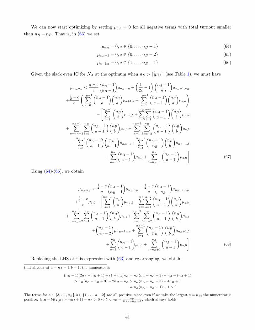
We can now start optimizing by setting µa,b = 0 for all negative terms with total turnout smaller

than nB + nB. That is, in (63) we set

µa,a = 0, a ∈ {0, . . . , nB − 1} (64)

µa,a+1 = 0, a ∈ {0, . . . , nB − 2} (65)

µa+1,a = 0, a ∈ {1, . . . , nB − 1} (66)

Given the slack even IC for NA at the optimum when nB > d12nAe (see Table 1), we must have

µnA,nB<

12 − cc

(nA − 1

nB − 1

)µnB ,nB

+

(1

2c− 1

)(nA − 1

nB

)µnB+1,nB

+12 − cc

(nB−1∑a=0

(nA − 1

a

)(nBa

)µa+1,a +

nB−1∑a=1

(nA − 1

a− 1

)(nBa

)µa,a

)

−

[nB−1∑b=1

(nBb

)µnA,b +

nB∑a=3

a−2∑b=1

(nA − 1

a− 1

)(nBb

)µa,b

+

nA−1∑a=nB+2

nB∑b=1

(nA − 1

a− 1

)(nBb

)µa,b +

nB−2∑a=1

nB∑b=a+2

(nA − 1

a− 1

)(nBb

)µa,b

+

nB−1∑a=1

(nA − 1

a− 1

)(nBa+ 1

)µa,a+1 +

nB−1∑b=1

(nA − 1

nB

)(nBb

)µnB+1,b

+

nB∑a=2

(nA − 1

a− 1

)µa,0 +

nA∑a=nB+1

(nA − 1

a− 1

)µa,0

](67)

Using (64)-(66), we obtain

µnA,nB<

12 − cc

(nA − 1

nB − 1

)µnB ,nB

+12 − cc

(nA − 1

nB

)µnB+1,nB

+12 − cc

µ1,0 −

[nB−1∑b=1

(nBb

)µnA,b +

nB∑a=3

a−2∑b=1

(nA − 1

a− 1

)(nBb

)µa,b

+

nA−1∑a=nB+2

nB∑b=1

(nA − 1

a− 1

)(nBb

)µa,b +

nB−2∑a=1

nB∑b=a+2

(nA − 1

a− 1

)(nBb

)µa,b

+

(nA − 1

nB − 2

)µnB−1,nB

+

nB−1∑b=1

(nA − 1

nB

)(nBb

)µnB+1,b

+

nB∑a=2

(nA − 1

a− 1

)µa,0 +

nA∑a=nB+1

(nA − 1

a− 1

)µa,0

](68)

Replacing the LHS of this expression with (63) and re-arranging, we obtain

that already at a = nA − 1, b = 1, the numerator is

(nB − 1)(2nA − nB + 1) + (1− nA)nB = nB(nA − nB + 3)− nA − (nA + 1)

> nB(nA − nB + 3)− 2nB − nA > nB(nA − nB + 3)− 4nB + 1

= nB(nA − nB − 1) + 1 > 0.

The terms for a ∈ {3, . . . , nB}, b ∈ {1, . . . , a− 2} are all positive, since even if we take the largest a = nB , the numerator ispositive: (nB − b)(2(nA − nB) + 1)− nB > 0⇔ b < nB − nB

2(nA−nB)+1, which always holds.

41

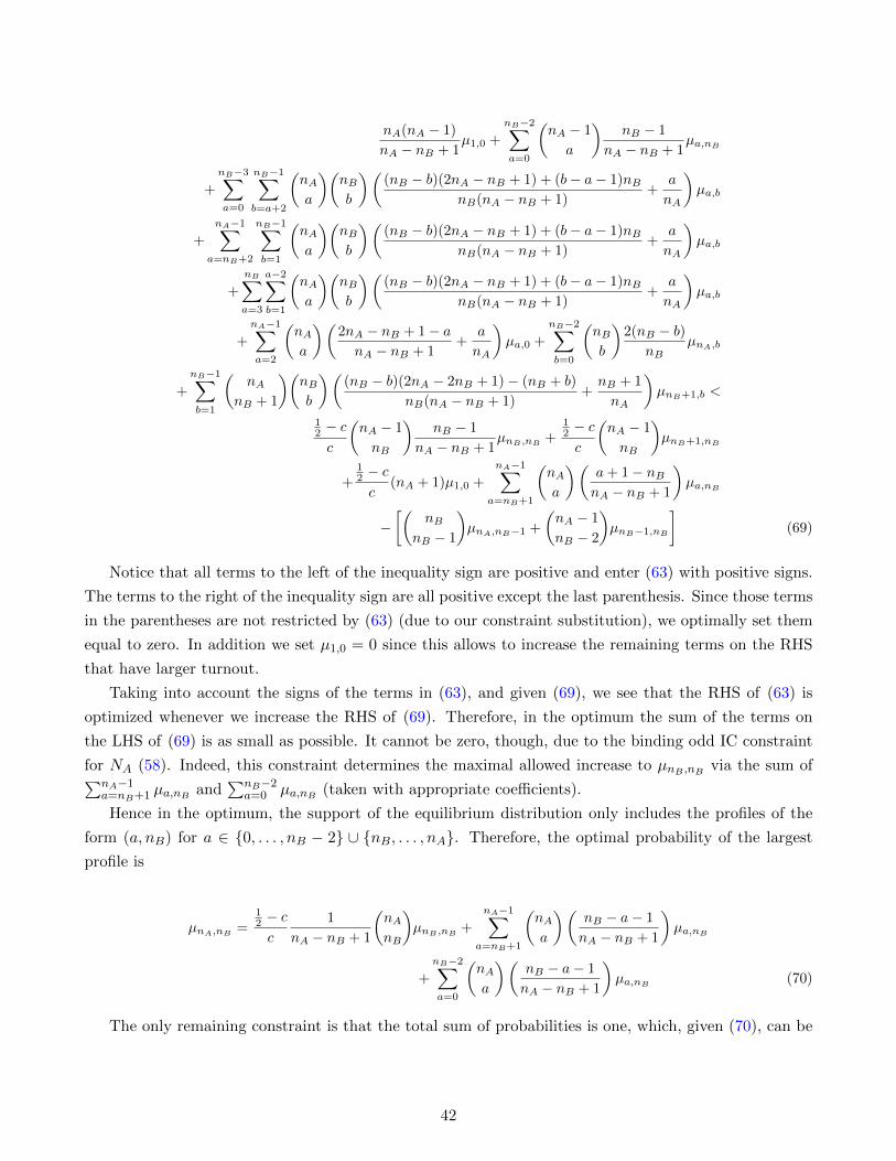
nA(nA − 1)

nA − nB + 1µ1,0 +

nB−2∑a=0

(nA − 1

a

)nB − 1

nA − nB + 1µa,nB

+

nB−3∑a=0

nB−1∑b=a+2

(nAa

)(nBb

)((nB − b)(2nA − nB + 1) + (b− a− 1)nB

nB(nA − nB + 1)+

a

nA

)µa,b

+

nA−1∑a=nB+2

nB−1∑b=1

(nAa

)(nBb

)((nB − b)(2nA − nB + 1) + (b− a− 1)nB

nB(nA − nB + 1)+

a

nA

)µa,b

+

nB∑a=3

a−2∑b=1

(nAa

)(nBb

)((nB − b)(2nA − nB + 1) + (b− a− 1)nB

nB(nA − nB + 1)+

a

nA

)µa,b

+

nA−1∑a=2

(nAa

)(2nA − nB + 1− anA − nB + 1

+a

nA

)µa,0 +

nB−2∑b=0

(nBb

)2(nB − b)

nBµnA,b

+

nB−1∑b=1

(nA

nB + 1

)(nBb

)((nB − b)(2nA − 2nB + 1)− (nB + b)

nB(nA − nB + 1)+nB + 1

nA

)µnB+1,b <

12 − cc

(nA − 1

nB

)nB − 1

nA − nB + 1µnB ,nB

+12 − cc

(nA − 1

nB

)µnB+1,nB

+12 − cc

(nA + 1)µ1,0 +

nA−1∑a=nB+1

(nAa

)(a+ 1− nBnA − nB + 1

)µa,nB

−[(

nBnB − 1

)µnA,nB−1 +

(nA − 1

nB − 2

)µnB−1,nB

](69)

Notice that all terms to the left of the inequality sign are positive and enter (63) with positive signs.

The terms to the right of the inequality sign are all positive except the last parenthesis. Since those terms

in the parentheses are not restricted by (63) (due to our constraint substitution), we optimally set them

equal to zero. In addition we set µ1,0 = 0 since this allows to increase the remaining terms on the RHS

that have larger turnout.

Taking into account the signs of the terms in (63), and given (69), we see that the RHS of (63) is

optimized whenever we increase the RHS of (69). Therefore, in the optimum the sum of the terms on

the LHS of (69) is as small as possible. It cannot be zero, though, due to the binding odd IC constraint

for NA (58). Indeed, this constraint determines the maximal allowed increase to µnB ,nB via the sum of∑nA−1a=nB+1 µa,nB and

∑nB−2a=0 µa,nB (taken with appropriate coefficients).

Hence in the optimum, the support of the equilibrium distribution only includes the profiles of the

form (a, nB) for a ∈ {0, . . . , nB − 2} ∪ {nB, . . . , nA}. Therefore, the optimal probability of the largest

profile is

µnA,nB=

12 − cc

1

nA − nB + 1

(nAnB

)µnB ,nB

+

nA−1∑a=nB+1

(nAa

)(nB − a− 1

nA − nB + 1

)µa,nB

+

nB−2∑a=0

(nAa

)(nB − a− 1

nA − nB + 1

)µa,nB

(70)

The only remaining constraint is that the total sum of probabilities is one, which, given (70), can be

42

written as

nB−2∑a=0

(nAa

)µa,nB

+

nA−1∑a=nB

(nAa

)µa,nB

+12 − cc

1

nA − nB + 1

(nAnB

)µnB ,nB

+

nA−1∑a=nB+1

(nAa

)(nB − a− 1

nA − nB + 1

)µa,nB

+

nB−2∑a=0

(nAa

)(nB − a− 1

nA − nB + 1

)µa,nB

= 1

Rewriting,

nAnA − nB + 1

(nB−2∑a=0

(nA − 1

a

)µa,nB

+

nA−1∑a=nB+1

(nA − 1

a

)µa,nB

)

+12c + nA − nBnA − nB + 1

(nAnB

)µnB ,nB

= 1

Using the binding odd IC constraint for NA, (58), we obtain

nA−1∑a=nB+1

(nA − 1

a

)µa,nB

+

nB−2∑a=0

(nA − 1

a

)µa,nB

−12 − cc

(nA − 1

nB

)µnB ,nB

= 0

Substituting into the previous expression, we obtain

µnB ,nB=

2c(nA

nB

) (71)

Hence

nA−1∑a=nB+1

(nA − 1

a

)µa,nB

+

nB−2∑a=0

(nA − 1

a

)µa,nB

=(1− 2c)(nA − nB)

nA(72)

Plugging-in these expressions into the objective function and simplifying, we rewrite (47) as

43

f∗ = 1 +

nB−2∑a=0

(nB + a− 1)

(nAa

)µa,nB

+

nA−1∑a=nB+1

(nB + a− 1)

(nAa

)µa,nB

+(nB + nB − 1)

(nAnB

)µnB ,nB

+ (nA + nB − 1)µnA,nB

= 1 +

nB−2∑a=0

(nB + a− 1)

(nAa

)µa,nB

+

nA−1∑a=nB+1

(nB + a− 1)

(nAa

)µa,nB

+(nB + nB − 1)2c+nA + nB − 1

nA − nB + 1

[1− 2c+

nA−1∑a=nB+1

(nAa

)(nB − a− 1)µa,nB

+

nB−2∑a=0

(nAa

)(nB − a− 1)µa,nB

]

= 1 + (2nB − 1)2c+(1− 2c)(nA + nB − 1)

nA − nB + 1+

2(nB − 1)nAnA − nB + 1

[nB−2∑a=0

(nA − 1

a

)µa,nB

+

nA−1∑a=nB+1

(nA − 1

a

)µa,nB

]

= 4cnB + (1− 2c)

[1 +

nA + nB − 1

nA − nB + 1+

2(nB − 1)nA(nA − nB)

(nA − nB + 1)nA

]= 4cnB + 2(1− 2c)nB

nA − nB + 1

nA − nB + 1= 2nB

So, the maximal expected turnout is twice the size of the minority.

This completes the proof of case (i), with the exception of the knife-edge case of nB = d12nAe. We

address this case after finishing the proof of case (ii).

Now suppose nB < d12nAe. Then 2nB < nA. Due to the odd IC for NA and even IC for NB binding,

we can express the probability of the largest profile as

µnA,nB=

12 − cc

(−

nB−2∑a=0

(nAa

)(nB − 1

a+ 1

)nA + 1


+

nB∑a=1

(nAa

)(nBa

)µa,a


))

+

nB−2∑a=0

nB∑b=a+2

(nAa

)(nBb

)((nB − b)(nA + 1) + (b− a− 1)nB

nB(nA − nB + 1)

)µa,b

+

nA−1∑a=nB+2

nB∑b=1

(nAa

)(nBb

)(nB(nA + b− a)− b(nA + 1)

nB(nA − nB + 1)

)µa,b

+

nB∑a=2

a−1∑b=1

(nAa

)(nBb

)(nB(nA + b− a)− b(nA + 1)

nB(nA − nB + 1)

)µa,b

+

nB∑b=1

(nA

nB + 1

)(nBb

)((nA − nB)(nB − b)− (nB + b)

nB(nA − nB + 1)

)µnB+1,b

+nA

nA − nB + 1

nA−1∑a=1

(nA − 1

a

)µa,0 −

nB−1∑b=1

(nB − 1

b− 1

)µnA,b (73)

44

On the other hand, the even IC for NA binding implies

µnA,nB=

12 − cc

(nB∑a=0

(nA − 1

a

)(nBa

)µa+1,a +

nB∑a=1

(nA − 1

a− 1

)(nBa

)µa,a

)

−

[nB−1∑b=1

(nBb

)µnA,b +

nB∑a=3

a−2∑b=1

(nA − 1

a− 1

)(nBb

)µa,b

+

nA−1∑a=nB+2

nB∑b=1

(nA − 1

a− 1

)(nBb

)µa,b +

nB−2∑a=1

nB∑b=a+2

(nA − 1

a− 1

)(nBb

)µa,b

]

−nB−1∑a=1

(nA − 1

a− 1

)(nBa+ 1

)µa,a+1 −

nB−1∑b=1

(nA − 1

nB

)(nBb

)µnB+1,b

−nA∑a=2

(nA − 1

a− 1

)µa,0 (74)

Comparing these two expressions and taking into account that the odd IC for NB is slack, we see that

at the optimum,

µa,a+1 = 0, a ∈ {0, . . . , nB − 1} (75)

µa,a = 0, a ∈ {0, . . . , nB − 1} (76)

µnB+1,b = 0, b ∈ {1, . . . , nB − 1} (77)

µa,b = 0, a ∈ {nB + 2, . . . , nA − 1}, b ∈ {0, . . . , nB} (78)

µa,b = 0, a ∈ {3, . . . , nB + 1}, b ∈ {1, . . . , a− 2} (79)

µa,b = 0, a ∈ {0, . . . , nB − 2}, b ∈ {a+ 2, . . . , nB} (80)

Given (75)-(80), we can rewrite (74) as

µnA,nB=

12 − cc

nB∑a=0

(nA − 1

a

)(nBa

)µa+1,a +

12 − cc

(nA − 1

nB − 1

)µnB ,nB

−nB−1∑b=1

(nBb

)µnA,b −

nB+1∑a=2

(nA − 1

a− 1

)µa,0 − µnA,0 (81)

We also rewrite (73) as

µnA,nB=

nB∑a=0

(nAa+ 1

)(nBa

)nB(nA − 1)− a(nA + 1)

nB(nA − nB + 1)µa+1,a −

nB−1∑b=1

(nB − 1

b− 1

)µnA,b

+

(12 − c

)nA

cnB(nA − nB + 1)

(nA − 1

nB − 1

)µnB ,nB

+nA

nA − nB + 1

nB+1∑a=2

(nA − 1

a

)µa,0 (82)

Now (81) and (82) imply that in the optimum

µnA,b = 0, b ∈ {1, . . . , nB − 1} (83)

45

In addition, the slack odd IC for NB, given (75)-(80), takes the form

µnA,0 +

nB+1∑a=2

(nAa

)µa,0 >

12 − cc

nB−1∑a=0

(nAa+ 1

)(nB − 1

a

)µa+1,a (84)

Together with 2nB ≤ nA − 1, this implies that at the optimum µa,0 = 0, a ∈ [2, nB + 1], and hence

the support of the distribution includes only the profiles of the form (a+ 1, a), a ∈ [0, nB], (nB, nB) and

(nA, 0). In particular, µnA,nB = 0, since from (84) and (81), µnA,0 offsets µnB+1,nB and µnB ,nB (from the

maximization point of view, the profiles with higher turnout must receive larger probability weights).

Hence we can rewrite (81) as

µnA,nB= 0 =

12 − cc

(nB∑a=0

(nA − 1

a

)(nBa

)µa+1,a +

(nA − 1

nB − 1

)µnB ,nB

)− µnA,0 (85)

The probability constraint now can be written as

nB∑a=0

(nAa+ 1

)(nBa

)µa+1,a +

(nAnB

)µnB ,nB

+12 − cc

(nB∑a=0

(nA − 1

a

)(nBa

)µa+1,a +

(nA − 1

nB − 1

)µnB ,nB

)= 1

Simplifying,

nB∑a=0

(nAa+ 1

)(nBa

)(nA + (a+ 1)( 1

2c − 1)

nA

)µa+1,a

+

(nA − 1

nB − 1

)(nAnB

+1

2c− 1

)µnB ,nB

= 1 (86)

From (82),

0 =

(nAnB

) 12c − 1


+

nB∑a=0

(nAa+ 1

)(nBa

)(nB(nA − 1)− a(nA + 1)

nB(nA − nB + 1)

)µa+1,a (87)

Thus

µnB ,nB= −

nB∑a=0

(nAa+ 1

)(nBa

)(nB(nA − 1)− a(nA + 1)

nB( 12c − 1)

(nA

nB

) )µa+1,a (88)

Now we can rewrite (86) as

nB∑a=0

(nAa+ 1

)(nBa

)µa+1,a

[nA + (a+ 1)( 1

2c − 1)

nA

−(nAnB

+1

2c− 1

)(nB(nA − 1)− a(nA + 1)

nA( 12c − 1)

)]= 1 (89)

46

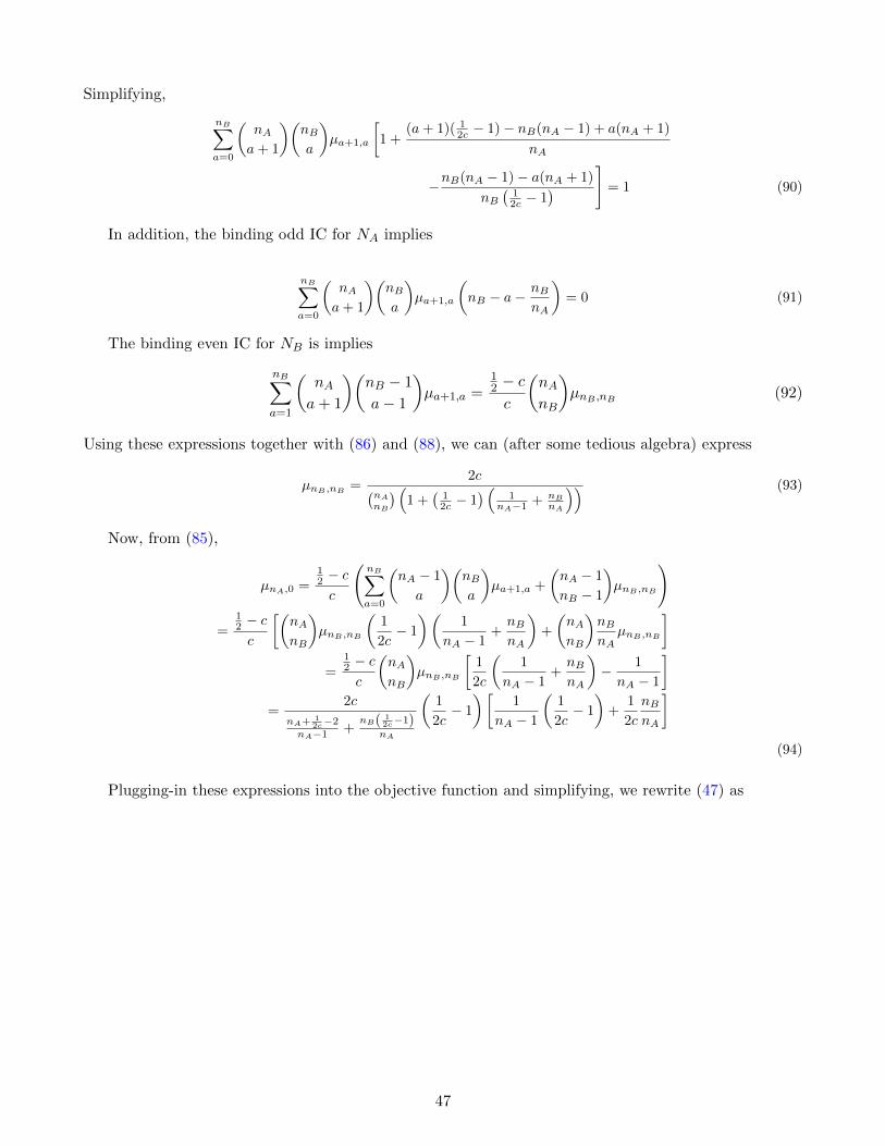
Simplifying,

nB∑a=0

(nAa+ 1

)(nBa

)µa+1,a

[1 +

(a+ 1)( 12c − 1)− nB(nA − 1) + a(nA + 1)

nA

−nB(nA − 1)− a(nA + 1)

nB(

12c − 1

) ]= 1 (90)

In addition, the binding odd IC for NA implies

nB∑a=0

(nAa+ 1

)(nBa

)µa+1,a

(nB − a−

nBnA

)= 0 (91)

The binding even IC for NB is implies

nB∑a=1

(nAa+ 1

)(nB − 1

a− 1

)µa+1,a =

12 − cc

(nAnB

)µnB ,nB (92)

Using these expressions together with (86) and (88), we can (after some tedious algebra) express

µnB ,nB=

2c(nA

nB

) (1 +

(12c − 1

) (1

nA−1 + nB

nA

)) (93)

Now, from (85),

µnA,0 =12 − cc

(nB∑a=0

(nA − 1

a

)(nBa

)µa+1,a +

(nA − 1

nB − 1

)µnB ,nB

)

=12 − cc

[(nAnB

)µnB ,nB

(1

2c− 1

)(1

nA − 1+nBnA

)+

(nAnB

)nBnA

µnB ,nB

]=

12 − cc

(nAnB

)µnB ,nB

[1

2c

(1

nA − 1+nBnA

)− 1

nA − 1

]=

2c

nA+ 12c−2

nA−1 +nB( 1

2c−1)nA

(1

2c− 1

)[1

nA − 1

(1

2c− 1

)+

1

2c

nBnA

](94)

Plugging-in these expressions into the objective function and simplifying, we rewrite (47) as

47

f∗ = 1 +

nB∑a=0

2a

(nAa+ 1

)(nBa

)µa+1,a + (2nB − 1)

(nAnB

)µnB ,nB

+ (nA − 1)µnA,0

= 1 +

nB∑a=0

2a

(nAa+ 1

)(nBa

)µa+1,a

−(2nB − 1)

(nAnB

) nB∑a=0

(nAa+ 1

)(nBa

)(nB(nA − 1)− a(nA + 1)

nB( 12c − 1)

(nA

nB

) )µa+1,a

+(nA − 1)12 − cc

(nB∑a=0

(nA − 1

a

)(nBa

)µa+1,a

−(nA − 1

nB − 1

) nB∑a=0

(nAa+ 1

)(nBa

) (nB(nA − 1)− a(nA + 1)

nB( 12c − 1)

(nA

nB

) )µa+1,a

)

= 1 +

nB∑a=0

(nAa+ 1

)(nBa

)µa+1,a

[2a− (2nB − 1)

nB(nA − 1)− a(nA + 1)

nB( 12c − 1)

+(nA − 2nB + 2nB − 1)(a+ 1)( 1

2c − 1)

nA− (nA − 2nB + 2nB − 1)

nB(nA − 1)− a(nA + 1)

nA

]= 1 +

nB∑a=0

(nAa+ 1

)(nBa

)µa+1,a

[2a− (2nB − 1)

nB(nA − 1)− a(nA + 1)

nB( 12c − 1)

+(2nB − 1)(a+ 1)( 1

2c − 1)

nA− (2nB − 1)

nB(nA − 1)− a(nA + 1)

nA

+(nA − 2nB)(a+ 1)( 1

2c − 1)

nA− (nA − 2nB)

nB(nA − 1)− a(nA + 1)

nA

]= 1 + 2nB − 1 +

nB∑a=0

(nAa+ 1

)(nBa

)µa+1,a

[2a− 2nB + 1

+(nA − 2nB)(a+ 1)( 1

2c − 1)− nB(nA − 1) + a(nA + 1)

nA

]= 2nB +

nA − 2nB2cnA

(1 + nB −

nBnA

) nB∑a=0

(nAa+ 1

)(nBa

)µa+1,a

= 2nB +nA − 2nB

2cnA

(1 + nB −

nBnA

)(1− µnA,0 −

(nAnB

)µnB ,nB

)= 2nB +

nA − 2nB2cnA

(1 + nB −

nBnA

)

×

nA+ 12c−2

nA−1 +nB( 1

2c−1)nA

− 2c(

12c − 1

) [1

nA−1

(12c − 1

)+ 1

2cnB

nA

]− 2c

nA+ 12c−2

nA−1 +nB( 1

2c−1)nA

= 2nB +

(nA − 2nB)(1− 2c)

1 + 2c(

nA(nA−1)nA+nB(nA−1) − 1

)= 2nB + φ(c)

= nA ×2cnB(nA − 1) + nB(nA − 1) + nA(1− 2c)

2c(nA − nB)(nA − 1) + nB(nA − 1) + nA(1− 2c)

= nA × ξ(c)

This completes the proof of case (ii).

Finally, there remains the knife-edge case of nB = d12nAe. When nA is odd, the odd IC for NB is

binding, so the proof of case (i) given above works just the same, giving the maximal expected turnout

48

of 2nB. When nA is even, the odd IC for NB is slack, so the proof of case (ii) directly applies. The

value of the objective function at the optimum has φ(c) = 0. However, in contrast to case (ii), the

support of the symmetric distribution is different and in fact, may include all profiles except the tied

ones with turnout less than nB, and the profiles of the form (a, a+ 1), a ∈ [0, nB − 1]. There is no simple

analytic expression available for the equilibrium support, so we verified our conclusions for this case using

computer simulations.

A.3 Proof of Corollary 3

Proof. Case (ii). In this case, the only profile in the support where the majority can lose is (nB, nB), so

πm = 1− 1

2

(nAnB

)µnB ,nB = 1− c

1 +(

12c − 1

) (1

nA−1 + nBnA

)Case (i). Since in the equilibrium distribution support all the profiles where the majority wins are of the

form (a, nB) for a ∈ [nB + 1, nA] plus the largest tied profile, it is easy to see that

πm =1

2

(nAnB

)µnB ,nB +

nA−1∑a=nB+1

(nAa

)µa,nB + µnA,nB (95)

The first term above equals c from (71), but we do not have enough constraints to identify the remaining

terms in the sum individually. The rest of the proof the bounds on these terms producing the result in

the statement.

As Table 1 shows, at the optimum there are three binding constraints plus the total sum of probabilities

constraint. It turns out that the first binding constraint, (58), becomes equation (72), which we repeat

here for convenience:

nB−2∑a=0

(nA − 1

a

)µa,nB +

nA−1∑a=nB+1

(nA − 1

a

)µa,nB = (1− 2c)

(1− nB

nA

)(96)

The second binding constraint, (59), becomes an identity as it does not contain any profiles from the

equilibrium support. The third binding constraint, (60), reduces to the total probability constraint.

Namely,

nB−2∑a=0

(nAa

)µa,nB +

(nAnB

)µnB ,nB +

nA∑a=nB+1

(nAa

)µa,nB = 1 (97)

From (71), 12

(nAnB

)µnB ,nB = c. Hence from the total probability constraint, 1 − πm − c ≥ 0 and the

first inequality in the statement follows.

The two binding constraints we are left with, (96) and (97), are not enough to determine πm even

knowing µnB ,nB . Nevertheless, from (96) and (97) we can express

µnA,nB =nBnA

(1− 2c)−nB−2∑a=0

a

nA

(nAa

)µa,nB −

nA−1∑a=nB+1

a

nA

(nAa

)µa,nB

49

Note that at the optimum µnA,nB > 0. We want to show that πm > 0.5 for all c ∈ (0, 0.5). Suppose by

way of contradiction that πm ≤ 0.5 for some cost c in this range. Then from (95)

µnA,nB+

nA−1∑a=nB+1

(nAa

)µa,nB

≤ 1

2(1− 2c)

Correspondingly, from (97)

nB−2∑a=0

(nAa

)µa,nB

≥ 1

2(1− 2c)

This implies that the total probability mass is greater on the lower turnout profiles than on the higher

turnout ones. Denote T the expected turnout at the optimal probability distribution. From Proposition

1, T = 2nB. Then

2nB =

nB−2∑a=0

(a+ nB)

(nAa

)µa,nB + 2c · 2nB +

nA∑a=nB+1

(a+ nB)

(nAa

)µa,nB

= (1− 2c)

(1

2+ ε

)µL + 2c · 2nB + (1− 2c)

(1

2− ε)µH ,

where µL is the mean expected turnout at the lower turnout profiles, µL ∈ (0, 2nB − 2); µH is the mean

expected turnout at the higher turnout profiles, µH ∈ (2nB + 1, nA + nB), and ε ∈ [0, 0.5) is such that

πm = 12 − ε. But then

2nB = (1− 2c)

[(1

2+ ε

)(µL + µH)− 2εµH

]+ 2c · 2nB < 2nB,

since due to 2nB > nA and turnout maximization,(

12 + ε

)(µL + µH) − 2εµH < 2nB. Contradiction, so

πm > 12 .


Proof. The results follow by taking the limits of the expressions for the maximal expected turnout ob-

tained in Proposition 1, divided by n ≡ nA + nB. To make sure the proof of Proposition 1 works in the

first place, notice that the incentive compatibility constraints (49)-(52) are well-behaved for all n and

bounded.


Proof. The minimum case is different, because the smallest (and so potentially optimal) profile (0, 0) ∈VT for all nA, nB ≥ 1. Nevertheless, the symmetric distribution construction derived in the proof of

Proposition 1 can be applied here just as well. Notice first that µ0,0 ≥ 0 at the optimum. Using the latter

50

and the fact that all profile probabilities sum up to one, rewrite the objective in (35) as

1− µ0,0 +∑

{s|∑si=2}

µ(s) + 2∑

{s|∑si=3}

µ(s) + . . .

+(n− 2)∑

{s|∑si=n−1}

µ(s) + (n− 1)µnA,nB (98)

To minimize this expression, we want to increase µ0,0 as much as possible and set all remaining

probabilities to their lowest possible level. Notice that profiles (0, 1) and (1, 0) are not directly present

in (98), and profiles with total turnout of exactly two have the same (absolute) marginal effect on the

objective as µ0,0.

The odd ICs for NA and NB, (49) and (51), respectively, restrict µ0,0 from above26, and the exact

bound depends on the ratio12−cc . This ratio approaches zero when the cost increases towards 0.5, so for

large enough cost, minimization requires placing the largest probability mass onto (0, 0) at the expense

of other voting profiles (in particular, with total turnout of three or more), and so the minimal expected

turnout approaches zero. The opposite happens when the cost is close to 0, because then12−cc → ∞,

and hence (49) and (51) both require their right hand sides being close to zero. Since nA ≥ nB, this

is achieved by setting µa,a = 0 for a ∈ {0, . . . , nB − 1}. The probability of the largest tied profile,

µnB ,nB , can be positive at the optimum for c close to zero, because12−cc

(nA−1nB−1

)µnB ,nB restricts µ2,0 from

above in the even IC for NA, (50), and12−cc

(nAnB

)µnB ,nB restricts µ0,2 from above in the even IC for NB,

(52), whereas for nA = nB, µnB ,nB is not at all restricted by the odd IC constraints (see ft.26), and for

nA > nB, µnB ,nB is only restricted by the odd IC for NA. But in all cases, the value of the objective does

not exceed 2: it is always optimal to shift the largest possible probability mass onto the profiles with

total turnout between 0 to 2, so even when c is close to 0, the (possible) presence of non-zero terms with

turnout exceeding 2 is compensated by their small equilibrium probabilities. The analytic expression

for the missing cost-dependent part of the expected turnout, ψ(c), can be now straightforwardly, though

rather tediously (due to the equilibrium distribution support depending on the cost) derived using the

same approach we applied in the proof of Proposition 1. For c close to 0, all IC constraints are binding,

while for c close to 0.5, all but the even IC for NB bind.


Proof. Any t ∈ [f∗(c), f∗(c)] can be written as a linear combination of f∗(c) and f∗(c): t = λf∗(c) + (1−

λ)f∗(c) for some λ ∈ [0, 1]. Since f∗(c), f∗(c) are expected turnouts in a min-turnout and max-turnout

correlated equilibria, and the set of CE payoffs is convex, t is also an expected turnout in some correlated

equilibrium given by probability distribution λµ∗ + (1− λ)µ∗.

A.7 Proof of Lemma 2

Proof. By way of contradiction, suppose there is a correlated equilibrium with majority winning for sure.

Then a profile (0, 0) is not in equilibrium support. The only way the IC constraint for voters in NB can

26If nA = nB , the right hand sides of the ICs for NA in (49) and (51) must be a bit adjusted to have the indices in thefirst summation go up to nB − 1 instead of nB .

51

be satisfied with a positive voting cost is to restrict the total probability mass to only those profiles where

no one from NB ever votes.27 This leaves admissible only profiles with voters from NA voting. Denote

ν(1i, a− 1, b) the equilibrium probability of a joint profile where i ∈ NA votes and there are a− 1 other

players from NA voting and b players from NB voting.28 The IC constraint for voter i from NA (see (6))

takes the following form:nA∑a=2

ν(1i, a− 1, 0) ≤12 − cc

ν(1i, 0, 0)

At the same time, the IC constraint for any non-voter from NB (see (5)) can be written as

nA∑a=2

∑i∈NA

ν(1i, a− 1, 0) ≥12 − cc

∑i∈NA

ν(1i, 0, 0)

Clearly, both constraints cannot be satisfied simultaneously. Hence there is no correlated equilibrium

with majority winning for sure.


Proof. Welfare maximizing correlated equilibria have Pr(Majority wins) as large as possible and expected

turnout as small as possible, so profiles of the form (a+ 1, a), a ∈ [0, nB] must be in the support. The IC

for non-voters in NB is now binding at the optimum and implies(nA2

)µ2,0 +

(nB − 1

1

)µ0,1 =

12 − cc

[nB−1∑a=0

(nAa

)(nB − 1

a

)µa,a +

nB−1∑a=0

(nAa+ 1

)(nB − 1

a

)µa+1,a

], (99)

hence the equilibrium profiles must also include either (2, 0), or (0, 1), or both. Note though that at (0, 1)

majority loses, so including this profile decreases the probability that majority wins as well as expected

welfare. It is also important that in (99) the probability of tied profiles restricts the probability mass

distributed among the welfare-optimal profiles (a+ 1, a), a ∈ [0, nB − 1], so there can be at most one tied

profile in the equilibrium: (nB, nB).

The odd IC constraint for NA implies

nB∑a=0

(nA − 1

a+ 1

)(nBa

)µa+1,a +

(nA − 1

2

)µ2,0 ≥

12 − cc

[(nA − 1

nB

)µnB ,nB

+

(nB1

)µ0,1

]

This constraint is always slack at the optimum since it does not restrict the total probability of the

welfare-maximizing profiles on the left hand side.

The even IC constraint for NA implies(nA − 1

1

)µ2,0 ≤

12 − cc

(nB∑a=0

(nA − 1

a

)(nBa

)µa+1,a +

(nA − 1

nB − 1

)µnB ,nB

)(100)

27Strictly speaking, in this case the conditional probability that a voting player from NB is pivotal is not well-defined, sothe corresponding IC constraint is vacuously satisfied.

28This is a shorthand notation, which should be understood as a sum of probabilities of all joint profiles where i is votingand all remaining players behave as described.

52

and is binding at the optimum due to (99). Finally, the even IC constraint for NB implies

nB∑a=1

(nAa+ 1

)(nB − 1

a− 1

)µa+1,a ≤

12 − cc

(µ0,1 +

(nAnB

)µnB ,nB

)(101)

This constraint can be satisfied if either (0, 1) or (nB, nB) are in the support29, in which case the constraint

is binding as long as some of the profiles (a + 1, a), a ∈ [1, nB] are in the support. If neither (0, 1) nor

(nB, nB) is in the support, the constraint requires all profiles (a+1, a), a ∈ [1, nB] not to be in the support

as well.

Rewriting (99), we obtain

(nA2

)µ2,0 +

(nB − 1

1

)µ0,1 =

12 − cc

nB−1∑a=0

(nAa+ 1

)(nB − 1

a

)µa+1,a (102)

From (100),

(nA − 1)µ2,0 =12 − cc

(nB∑a=0

(nA − 1

a

)(nBa

)µa+1,a +

(nA − 1

nB − 1

)µnB ,nB

)(103)

so we can rewrite (102) as

12 − cc

[nB−1∑a=0

[(nAa+ 1

)(nB − 1

a

)−

(nA

2

)nA − 1

(nA − 1

a

)(nBa

)]µa+1,a

]=

12 − cc

(nA

2

)nA − 1

((nA − 1

nB

)µnB+1,nB

+

(nA − 1

nB − 1

)µnB ,nB

)+ (nB − 1)µ0,1

or

12 − c

2cnAµ1,0 +

12 − c

2c

nB∑a=1

(nAa+ 1

)(nBa

)(1− a

(1 +

2

nB

))µa+1,a =

12 − cc

(nAnB

)nB2µnB ,nB

+ (nB − 1)µ0,1 (104)

Notice that all terms in the sum on the first line are negative if profiles (a + 1, a), a ∈ [1, nB] are in the

support.

The total probability constraint takes the following form:

nB∑a=0

(nAa+ 1

)(nBa

)µa+1,a +

(nA2

)µ2,0 +

(nB1

)µ0,1 +

(nAnB

)µnB ,nB

= 1

Plugging in the expression for µ2,0 from (103), we obtain

nB∑a=0

(nAa+ 1

)(nBa

)µa+1,a

[1 +

( 12 − c)(a+ 1)

2c

]+

(nAnB

)µnB ,nB

[nB( 1

2 − c)2c

+ 1

]+ nBµ0,1 = 1 (105)

Using the total probability constraint, the total welfare minus the fixed nB term can be written as

29It is not optimal to include both profiles in the support, because then there is simultaneously a decrease in the probabilitymajority wins and an increase in the expected turnout.

53

follows

W − nB = (nA − nB)

[1− 1

2

(nAnB

)µnB ,nB

− nBµ0,1

]−c

[nB∑a=0

(2a+ 1)

(nAa+ 1

)(nBa

)µa+1,a + 2

(nA2

)µ2,0 + 2nB

(nAnB

)µnB ,nB

+ nBµ0,1

]

Suppose all profiles (a+ 1, a), a ∈ [1, nB] are in the support, then IC constraint (101) is binding:

nB∑a=0

a

(nAa+ 1

)(nBa

)µa+1,a =

12 − cc

(nBµ0,1 + nB

(nAnB

)µnB ,nB

)(106)

Thus we can rewrite the above expression for welfare as

W − nB = (nA − nB)

[1− 1

2

(nAnB

)µnB ,nB

− nBµ0,1

]−c[

2( 12 − c)c

(nBµ0,1 + nB

(nAnB

)µnB ,nB

)+ 1 +

(nA2

)µ2,0 + (2nB − 1)

(nAnB

)µnB ,nB

]Simplifying, this equals

= nA − nB − c+

(nAnB

)µnB ,nB

[c− nA + nB

2

]+ nBµ0,1 [2c+ nB − nA − 1]− c

(nA2

)µ2,0

Plugging in the expression for µ2,0, we obtain

nA − nB − c+

(nAnB

)µnB ,nB

[c− nA + nB

2−nB( 1

2 − c)2

]+ nBµ0,1 [2c+ nB − nA − 1]

−12 − c

2

(nB∑a=0

(nAa+ 1

)(nBa

)(a+ 1)µa+1,a

)

After tedious algebraic manipulations with the binding IC constraints, we can express the sum of all

(a+ 1, a) profile probabilities as follows.

12 − c

2c

nB∑a=0

(nAa+ 1

)(nBa

)µa+1,a = µ0,1

[nB − 1 +

( 12 − cc

)2

(1 +nB2

)

]

+

(nAnB

)µnB ,nB

[( 12 − cc

)2

(1 +nB2

) +nB( 1

2 − c)2c

]

Using this expression together with (106) to substitute the respective terms in the formula for welfare,

we obtain

W = nA − c+

(nAnB

)µnB ,nB

[c− nA + nB

2−nB( 1

2 − c)2

]+ nBµ0,1 [2c+ nB − nA − 1]

−c

[µ0,1

[nB − 1 +

( 12 − cc

)2

(1 +nB2

)

]+

(nAnB

)µnB ,nB

[( 12 − cc

)2

(1 +nB2

) +nB( 1

2 − c)2c

]]

−12 − c

2

12 − cc

(nBµ0,1 + nB

(nAnB

)µnB ,nB

)

54

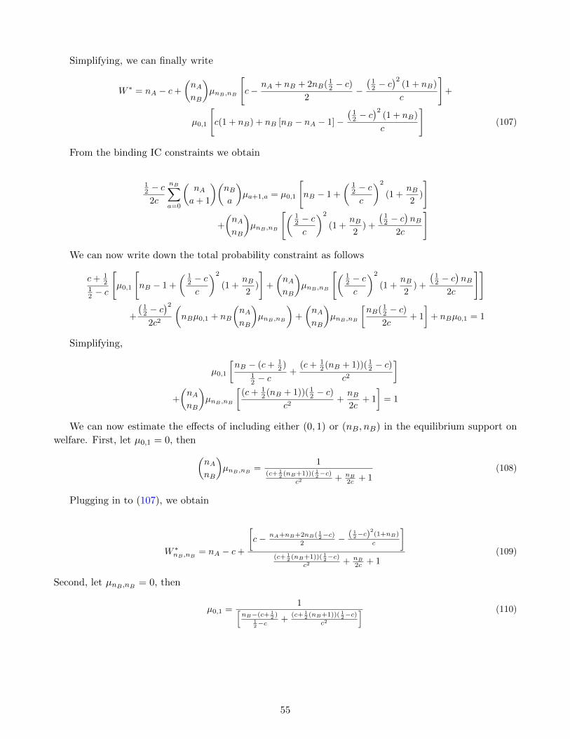
Simplifying, we can finally write

W ∗ = nA − c+

(nAnB

)µnB ,nB

[c−

nA + nB + 2nB( 12 − c)

2−(

12 − c

)2(1 + nB)

c

]+

µ0,1

[c(1 + nB) + nB [nB − nA − 1]−

(12 − c

)2(1 + nB)

c

](107)

From the binding IC constraints we obtain

12 − c

2c

nB∑a=0

(nAa+ 1

)(nBa

)µa+1,a = µ0,1

[nB − 1 +

( 12 − cc

)2

(1 +nB2

)

]

+

(nAnB

)µnB ,nB

[( 12 − cc

)2

(1 +nB2

) +

(12 − c

)nB

2c

]

We can now write down the total probability constraint as follows

c+ 12

12 − c

[µ0,1

[nB − 1 +

( 12 − cc

)2

(1 +nB2

)

]+

(nAnB

)µnB ,nB

[( 12 − cc

)2

(1 +nB2

) +

(12 − c

)nB

2c

]]

+

(12 − c

)22c2

(nBµ0,1 + nB

(nAnB

)µnB ,nB

)+

(nAnB

)µnB ,nB

[nB( 1

2 − c)2c

+ 1

]+ nBµ0,1 = 1

Simplifying,

µ0,1

[nB − (c+ 1

2 )12 − c

+(c+ 1

2 (nB + 1))( 12 − c)

c2

]+

(nAnB

)µnB ,nB

[(c+ 1

2 (nB + 1))( 12 − c)

c2+nB2c

+ 1

]= 1

We can now estimate the effects of including either (0, 1) or (nB, nB) in the equilibrium support on

welfare. First, let µ0,1 = 0, then(nAnB

)µnB ,nB

=1

(c+ 12 (nB+1))( 1

2−c)c2 + nB

2c + 1(108)

Plugging in to (107), we obtain

W ∗nB ,nB= nA − c+

[c− nA+nB+2nB( 1

2−c)2 − ( 1

2−c)2(1+nB)

c

](c+ 1

2 (nB+1))( 12−c)

c2 + nB

2c + 1(109)

Second, let µnB ,nB = 0, then

µ0,1 =1[

nB−(c+ 12 )

12−c

+(c+ 1

2 (nB+1))( 12−c)

c2

] (110)

55

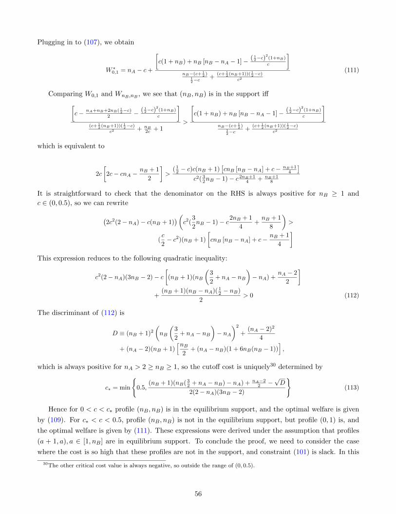
Plugging in to (107), we obtain

W ∗0,1 = nA − c+

[c(1 + nB) + nB [nB − nA − 1]− ( 1

2−c)2(1+nB)

c

]nB−(c+ 1

2 )12−c

+(c+ 1

2 (nB+1))( 12−c)

c2

(111)

Comparing W0,1 and WnB ,nB , we see that (nB, nB) is in the support iff[c− nA+nB+2nB( 1

2−c)2 − ( 1

2−c)2(1+nB)

c

](c+ 1

2 (nB+1))( 12−c)

c2 + nB

2c + 1>

[c(1 + nB) + nB [nB − nA − 1]− ( 1

2−c)2(1+nB)

c

]nB−(c+ 1

2 )12−c

+(c+ 1

2 (nB+1))( 12−c)

c2

which is equivalent to

2c

[2c− cnA −

nB + 1

2

]>

( 12 − c)c(nB + 1)

[cnB [nB − nA] + c− nB+1

4

]c2( 3

2nB − 1)− c 2nB+14 + nB+1

8

It is straightforward to check that the denominator on the RHS is always positive for nB ≥ 1 and

c ∈ (0, 0.5), so we can rewrite

(2c2(2− nA)− c(nB + 1)

)(c2(

3

2nB − 1)− c2nB + 1

4+nB + 1

8

)>

(c

2− c2)(nB + 1)

[cnB [nB − nA] + c− nB + 1

4

]This expression reduces to the following quadratic inequality:

c2(2− nA)(3nB − 2)− c[(nB + 1)(nB

(3

2+ nA − nB

)− nA) +

nA − 2

2

]+

(nB + 1)(nB − nA)( 12 − nB)

2> 0 (112)

The discriminant of (112) is

D ≡ (nB + 1)2

(nB

(3

2+ nA − nB

)− nA

)2

+(nA − 2)2

4

+ (nA − 2)(nB + 1)[nB

2+ (nA − nB)(1 + 6nB(nB − 1))

],

which is always positive for nA > 2 ≥ nB ≥ 1, so the cutoff cost is uniquely30 determined by

c∗ = min

{0.5,

(nB + 1)(nB( 32 + nA − nB)− nA) + nA−2

2 −√D

2(2− nA)(3nB − 2)

}(113)

Hence for 0 < c < c∗ profile (nB, nB) is in the equilibrium support, and the optimal welfare is given

by (109). For c∗ < c < 0.5, profile (nB, nB) is not in the equilibrium support, but profile (0, 1) is, and

the optimal welfare is given by (111). These expressions were derived under the assumption that profiles

(a + 1, a), a ∈ [1, nB] are in equilibrium support. To conclude the proof, we need to consider the case

where the cost is so high that these profiles are not in the support, and constraint (101) is slack. In this

30The other critical cost value is always negative, so outside the range of (0, 0.5).

56

case, of course, (nB, nB) is not in the equilibrium support.

Suppose that profiles (a+ 1, a), a ∈ {1, . . . , nB} are not in the equilibrium support. Then from (104),

12 − cc

µ1,0 =2(nB − 1)

nAµ0,1

Using the total probability constraint, we can now write(nA1

)µ1,0 +

(nA2

)µ2,0 +

(nB1

)µ0,1 = 1

or

µ0,1

[2(nB − 1)

12−cc

+ 2nB − 1

]= 1

So we obtain

µ0,1 =12 − c

nB −(

12 + c

)µ1,0 =

2c(nB − 1)

nA[nB −

(12 + c

)]µ2,0 =

(12 − c

)(nB − 1)(

nA

2

) [nB −

(12 + c

)]and the optimal welfare is

W ∗ =nB(nB − c)( 1

2 − c) + 2c(nB − 1)(nA − c) + (nA − 2c)(

12 − c

)(nB − 1)

nB −(

12 + c

) (114)

We can now compare W ∗ with W ∗0,1 to obtain the condition on the cost for which (a+1, a), a ∈ [1, nB]

are not in the support: this is so iff

nA − c+

( 12 − c)c

2

[c(1 + nB) + nB [nB − nA − 1]− ( 1

2−c)2(1+nB)

c

]c2(nB − (c+ 1

2 )) + (c+ 12 (nB + 1))( 1

2 − c)2<

nB(nB − c)( 12 − c) + 2c(nB − 1)(nA − c) + (nA − 2c)

(12 − c

)(nB − 1)

nB −(

12 + c

)which is equivalent to the following cubic inequality:

c3(nA +

nB − 5

2

)+c2

2((nA − nB)(nB − 1) + 3− nB)

− c4

(nB + 1

2+ (nA − nB)(2nB + 1)

)+

(nA − nB)(nB + 1)

8< 0


Proof. The proof closely follows the proof of Proposition 1. Assume that the optimal correlated equilib-

rium distribution is symmetric, as defined there. Although the voting costs are heterogenous, it is easy

57

to see that once constraints (38) hold for the players with the lowest cost in each group, and constraints

(39) hold for the players with the highest cost, the incentive compatibility constraints for all players will

hold automatically.

Using symmetry, we obtain the following system of four inequalities with respect to (nA + 1)(nB + 1)

variables of the form µa,b:

nA−1∑a=1

min{a−1,nB}∑b=0

(nA − 1

a

)(nBb

)µa,b +

nB−2∑a=0

nB∑b=a+2

(nA − 1

a

)(nBb

)µa,b ≥

12 − cAcA

(nB∑a=0

(nA − 1

a

)(nBa

)µa,a +

nB−1∑a=0

(nA − 1

a

)(nBa+ 1

)µa,a+1

)(115)

nA∑a=2

min{a−2,nB}∑b=0

(nA − 1

a− 1

)(nBb

)µa,b +

nB−1∑a=1

nB∑b=a+1

(nA − 1

a− 1

)(nBb

)µa,b ≤

12 − cAcA

(nB∑a=0

(nA − 1

a

)(nBa

)µa+1,a +

nB∑a=1

(nA − 1

a− 1

)(nBa

)µa,a

)(116)

and

nA∑a=2

min{a−2,nB−1}∑b=0

(nAa

)(nB − 1

b

)µa,b +

nB−2∑a=0

nB−1∑b=a+1

(nAa

)(nB − 1

b

)µa,b ≥

12 − cBcB

(nB−1∑a=0

(nAa

)(nB − 1

a

)µa,a +

nB−1∑a=0

(nAa+ 1

)(nB − 1

a

)µa+1,a

)(117)

nA∑a=2

min{a−1,nB}∑b=1

(nAa

)(nB − 1

b− 1

)µa,b +

nB−2∑a=0

nB∑b=a+2

(nAa

)(nB − 1

b− 1

)µa,b ≤

12 − cBcB

(nB−1∑a=0

(nAa

)(nB − 1

a

)µa,a+1 +

nB∑a=1

(nAa

)(nB − 1

a− 1

)µa,a

)(118)

We will refer to the first and the third inequality above as the odd incentive compatibility (IC) constraints,

and to the second and the fourth inequality as the even IC constraints, distinguished by the group.

Since nA > nB, at the largest turnout profile µnA,nB all voters from NB (as well as voters from NA,

if nA > nB + 1) are dummies. Hence the even IC constraint for NB is always binding at the optimum.

58

The even IC constraint for NA requires

µnA,nB≤

12 − cAcA

(nB−1∑a=0

(nA − 1

a

)(nBa

)µa+1,a +

nB∑a=1

(nA − 1

a− 1

)(nBa

)µa,a

)

−

[nB−1∑b=1

(nBb

)µnA,b +

nB∑a=3

a−2∑b=1

(nA − 1

a− 1

)(nBb

)µa,b

+

nA−1∑a=nB+2

nB∑b=1

(nA − 1

a− 1

)(nBb

)µa,b +

nB−2∑a=1

nB∑b=a+2

(nA − 1

a− 1

)(nBb

)µa,b

]

−nB−1∑a=1

(nA − 1

a− 1

)(nBa+ 1

)µa,a+1 −

nB∑b=1

(nA − 1

nB

)(nBb

)µnB+1,b −

nB∑a=2

(nA − 1

a− 1

)µa,0

+1

2cA

(nA − 1

nB

)µnB+1,nB

−nA∑

a=nB+1

(nA − 1

a− 1

)µa,0 (119)

The binding even IC for NB requires

µnA,nB=

12 − cBcB

(nB−1∑a=0

(nAa

)(nB − 1

a

)µa,a+1 +

nB∑a=1

(nAa

)(nB − 1

a− 1

)µa,a

)

−

[nB−1∑b=1

(nB − 1

b− 1

)µnA,b +

nB∑a=3

a−2∑b=1

(nAa

)(nB − 1

b− 1

)µa,b

+

nA−1∑a=nB+2

nB∑b=1

(nAa

)(nB − 1

b− 1

)µa,b +

nB−2∑a=1

nB∑b=a+2

(nAa

)(nB − 1

b− 1

)µa,b

]

−nB−1∑a=1

(nAa+ 1

)(nB − 1

a− 1

)µa+1,a −

nB∑b=1

(nA

nB + 1

)(nB − 1

b− 1

)µnB+1,b

−nB∑b=2

(nB − 1

b− 1

)µ0,b (120)

These expressions immediately imply that the odd IC for NA is always binding at the optimum. To

see this, notice that in the binding constraint (120) all profiles relevant for the odd IC for NA, i.e. those

where a non-voter from NA is a dummy, have the negative sign and so must be reduced as much as

possible at the optimum. The only subset of profiles where a non-voter from NA is a dummy that is not

directly restricted by (120) has the form∑nA−1

a=1

(nA−1a−1

)µa,0. But these profiles are restricted by (119). If

the latter is binding, the restriction is trivial. Suppose not, then if we reduced all directly restricted by

(120) probabilities to their lower limit of zero and the odd IC for NA was still not binding, then constraint

(119) (slack by assumption) would imply that µnA,nB < 0. Therefore, the odd IC for NA must bind at

59

the optimum, so we can write it as

nA−1∑a=nB+1

(nA − 1

a

)µa,nB

−12 − cAcA

(nA − 1

nB

)µnB ,nB

+

(nA − 1

nB

)(nB

nB − 1

)µnB ,nB−1 +

nB−2∑a=0

(nA − 1

a

)µa,nB

+

nB−2∑a=0

(nA − 1

a+ 1

)(nBa

)µa+1,a +

nB+1∑a=2

a−2∑b=0

(nA − 1

a

)(nBb

)µa,b

+

nA−1∑a=nB+2

nB−1∑b=0

(nA − 1

a

)(nBb

)µa,b +

nB−3∑a=0

nB−1∑b=a+2

(nA − 1

a

)(nBb

)µa,b =

12 − cAcA

(nB−1∑a=0

(nA − 1

a

)(nBa

)µa,a +

nB−1∑a=0

(nA − 1

a

)(nBa+ 1

)µa,a+1

)(121)

Thus for all cost thresholds the even IC for NB and the odd IC for NA are binding. Proceeding

exactly as in the proof of Proposition 1, we can express µnA,nB from (120) (the binding even IC for NB)

and then substitute the term(nA−1nB−1

)µnB−1,nB using (121) (the binding odd IC for NA). The resulting

expressions are the modified versions of (60), (61), and (62), respectively:

µnA,nB=

12 − cBcB

(nB−1∑a=0

(nAa

)(nB − 1

a

)µa,a+1 +

nB∑a=1

(nAa

)(nB − 1

a− 1

)µa,a

)

−

[nB−1∑b=1

(nB − 1

b− 1

)µnA,b +

nB∑a=2

a−1∑b=1

(nAa

)(nB − 1

b− 1

)µa,b

+

nA−1∑a=nB+1

nB∑b=1

(nAa

)(nB − 1

b− 1

)µa,b +

nB−2∑a=0

nB∑b=a+2

(nAa

)(nB − 1

b− 1

)µa,b

], (122)

(nA − 1

nB − 1

)· µnB−1,nB

=cA

12 − cA

[nB+1∑a=1

a−1∑b=0

(nA − 1

a

)(nBb

)µa,b

+

nA−1∑a=nB+2

nB∑b=0

(nA − 1

a

)(nBb

)µa,b +

nB−2∑a=0

nB∑b=a+2

(nA − 1

a

)(nBb

)µa,b

]

−

(nB∑a=0

(nA − 1

a

)(nBa

)µa,a +

nB−2∑a=0

(nA − 1

a

)(nBa+ 1

)µa,a+1

), (123)

60

and

µnA,nB=

12 − cBcB

(−

nB−2∑a=0

(nAa

)(nB − 1

a+ 1

)nA + 1


+

nB∑a=1

(nAa

)(nBa

)a(nA + 1)− nBnAnB(nA − nB + 1)

µa,a

)

−

[nB−1∑b=1

(nB − 1

b− 1

)µnA,b +

nB∑a=2

a−1∑b=1

(nAa

)(nB − 1

b− 1

)µa,b

+

nA−1∑a=nB+1

nB∑b=1

(nAa

)(nB − 1

b− 1

)µa,b +

nB−2∑a=0

nB∑b=a+2

(nAa

)(nB − 1

b− 1

)µa,b

]

+12 − cBcB

cA(12 − cA

) nAnA − nB + 1

[nB+1∑a=1

a−1∑b=0

(nA − 1

a

)(nBb

)µa,b

+

nA−1∑a=nB+2

nB∑b=0

(nA − 1

a

)(nBb

)µa,b +

nB−2∑a=0

nB∑b=a+2

(nA − 1

a

)(nBb

)µa,b

](124)

The key difference between (124) and (62) is that in (124), all terms in the last square brackets have

an additional multiplier12−cBcB

cA( 1

2−cA)

. The equivalence between (124) and (62) holds if and only if this

multiplier equals 1, that is, if and only if cA = cB. If these cost thresholds are different, the equilibrium

probability of the largest profile, as well as other profiles in the equilibrium support, will be different than

in either of the cases considered in Proposition 1, and therefore, the corresponding maximal expected

turnout will be different from f∗, the maximal expected turnout in Proposition 1. How much different

depends on the relation between cA and cB. Suppose that cA < cB. Then a simple contradiction argument

implies12 − cBcB

cA(12 − cA

) < 1 (125)

In this case, maximization implies placing a smaller probability mass on the largest turnout profile than in

Proposition 1.31 Therefore, the expected turnout is lower than in Proposition 1 for all costs satisfying this

condition. It is easy to show that if cA > cB, the opposite inequality holds in (125) and the equilibrium

distribution places a larger mass on µnA,nB , so the expected turnout is higher than in Proposition 1.

We will now show that if cA = cB, the equilibrium distribution support does not change, and the

maximal expected turnout corresponds to f∗ from Proposition 1.32

The remaining IC constraints, the even IC for NA and the odd IC for NB, generally exhibit more

complicated bind/slack properties. Unlike the homogenous cost case, their behavior at the optimum

depends on the relations between the cost thresholds. We claim, however, that if cA = cB = c, the IC

constraints exhibit the same behavior as in Proposition 1: for nB > d12nAe the even IC for NA is slack

for all admissible values of c and the remaining cost thresholds, cA and cB, and the odd IC for NB is

binding. For nB < d12nAe the even IC for NA is binding, and the odd IC for NB is slack.

Let nB > d12nAe. Comparing (120) and (119), we see that the RHS of (120) cannot be strictly greater

than the RHS of (119), since if this was the case, the even IC for NA would not hold at all at the optimum

31Note that this is true even if µnA,nB = 0 at the optimum, because in this case decreasing the RHS of (124) meanssmaller probability of the next largest profile in the equilibrium support.

32This is exactly so for case (i), where the expected turnout does not depend on the cost. For case(ii), which is costdependent, we will show that the expected turnout exhibits the same cost-dependent dynamics as in Proposition 1.

61

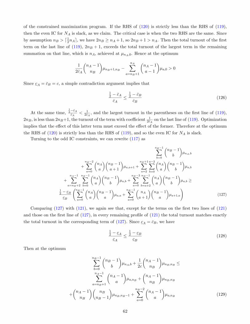
of the constrained maximization program. If the RHS of (120) is strictly less than the RHS of (119),

then the even IC for NA is slack, as we claim. The critical case is when the two RHS are the same. Since

by assumption nB > d12nAe, we have 2nB ≥ nA + 1, so 2nB + 1 > nA. Then the total turnout of the first

term on the last line of (119), 2nB + 1, exceeds the total turnout of the largest term in the remaining

summation on that line, which is nA, achieved at µnA,0. Hence at the optimum

1

2cA

(nA − 1

nB

)µnB+1,nB −

nA∑a=nB+1

(nA − 1

a− 1

)µa,0 > 0

Since cA = cB = c, a simple contradiction argument implies that

12 − cAcA

≤12 − cBcB

(126)

At the same time,12−cAcA

< 12cA

, and the largest turnout in the parentheses on the first line of (119),

2nB, is less than 2nB+1, the turnout of the term with coefficient 12cA

on the last line of (119). Optimization

implies that the effect of this latter term must exceed the effect of the former. Therefore at the optimum

the RHS of (120) is strictly less than the RHS of (119), and so the even IC for NA is slack.

Turning to the odd IC constraints, we can rewrite (117) as

nB−1∑b=0

(nB − 1

b

)µnA,b

+

nB−2∑a=0

(nAa

)(nB − 1

a+ 1

)µa,a+1 +

nB+1∑a=2

a−2∑b=0

(nAa

)(nB − 1

b

)µa,b

+

nA−1∑a=nB+2

nB−1∑b=0

(nAa

)(nB − 1

b

)µa,b +

nB−3∑a=0

nB−1∑b=a+2

(nAa

)(nB − 1

b

)µa,b ≥

12 − cBcB

(nB−1∑a=0

(nAa

)(nB − 1

a

)µa,a +

nB−1∑a=0

(nAa+ 1

)(nB − 1

a

)µa+1,a

)(127)

Comparing (127) with (121), we again see that, except for the terms on the first two lines of (121)

and those on the first line of (127), in every remaining profile of (121) the total turnout matches exactly

the total turnout in the corresponding term of (127). Since cA = cB, we have

12 − cAcA

≤12 − cBcB

(128)

Then at the optimum

nB−1∑b=0

(nB − 1

b

)µnA,b +

1

2c

(nA − 1

nB

)µnB ,nB ≤

nA−1∑a=nB+1

(nA − 1

a

)µa,nB +

(nA − 1

nB

)µnB ,nB

+

(nA − 1

nB

)(nB

nB − 1

)µnB ,nB−1 +

nB−2∑a=0

(nA − 1

a

)µa,nB (129)

62

This follows, since nB > d12nAe, so 2nB ≥ nA+ 1 and all profiles on the LHS of (129) are matched by the

corresponding profiles on the RHS. Together with (128), this implies that the odd IC for NB is binding.

We can now proceed exactly as in the proof of Proposition 1. One can even show that the expression

for the probability of the largest tie remains the same:

µnB ,nB=

2c(nA

nB

) , (130)

where c = cA = cB. Substituting the expressions for the probabilities of the largest profiles into the

objective function, we obtain h∗ = 2nB. This completes the proof of case (i).

Now suppose nB < d12nAe, then 2nB < nA. Analogously to case (ii) of Proposition 1, we have the

even IC for NA binding and the odd IC for NB slack at the optimum, if cA = cB = c. Due to the odd IC

for NA and the even IC for NB binding33, we can express the probability of the largest profile as

µnA,nB=

12 − cc

(−

nB−2∑a=0

(nAa

)(nB − 1

a+ 1

)nA + 1


+

nB∑a=1

(nAa

)(nBa

)µa,a


))

+

nB−2∑a=0

nB∑b=a+2

(nAa

)(nBb

)((nB − b)(nA + 1) + (b− a− 1)nB

nB(nA − nB + 1)

)µa,b

+

nA−1∑a=nB+2

nB∑b=1

(nAa

)(nBb

)(nB(nA + b− a)− b(nA + 1)

nB(nA − nB + 1)

)µa,b

+

nB∑a=2

a−1∑b=1

(nAa

)(nBb

)(nB(nA + b− a)− b(nA + 1)

nB(nA − nB + 1)

)µa,b

+

nB∑b=1

(nA

nB + 1

)(nBb

)((nA − nB)(nB − b)− (nB + b)

nB(nA − nB + 1)

)µnB+1,b

+nA

nA − nB + 1

nA−1∑a=1

(nA − 1

a

)µa,0 −

nB−1∑b=1

(nB − 1

b− 1

)µnA,b (131)

On the other hand, the even IC for NA binding implies

µnA,nB=

12 − cAcA

(nB∑a=0

(nA − 1

a

)(nBa

)µa+1,a +

nB∑a=1

(nA − 1

a− 1

)(nBa

)µa,a

)

−

[nB−1∑b=1

(nBb

)µnA,b +

nB∑a=3

a−2∑b=1

(nA − 1

a− 1

)(nBb

)µa,b

+

nA−1∑a=nB+2

nB∑b=1

(nA − 1

a− 1

)(nBb

)µa,b +

nB−2∑a=1

nB∑b=a+2

(nA − 1

a− 1

)(nBb

)µa,b

]

−nB−1∑a=1

(nA − 1

a− 1

)(nBa+ 1

)µa,a+1 −

nB−1∑b=1

(nA − 1

nB

)(nBb

)µnB+1,b

−nA∑a=2

(nA − 1

a− 1

)µa,0 (132)

33These constraints bind for case (i) just as well.

63

Comparing (132) with (131), taking into account that cA ≥ c and the odd IC for NB is slack, we see

that at the optimum, just like in case (ii) of Proposition 1,

µa,a+1 = 0, a ∈ {0, . . . , nB − 1} (133)

µa,a = 0, a ∈ {0, . . . , nB − 1} (134)

µnB+1,b = 0, b ∈ {1, . . . , nB − 1} (135)

µa,b = 0, a ∈ {nB + 2, . . . , nA − 1}, b ∈ {0, . . . , nB} (136)

µa,b = 0, a ∈ {3, . . . , nB + 1}, b ∈ {1, . . . , a− 2} (137)

µa,b = 0, a ∈ {0, . . . , nB − 2}, b ∈ {a+ 2, . . . , nB} (138)

Given (133)-(138), we can rewrite (132) as

µnA,nB=

12 − cAcA

nB∑a=0

(nA − 1

a

)(nBa

)µa+1,a +

12 − cAcA

(nA − 1

nB − 1

)µnB ,nB

−nB−1∑b=1

(nBb

)µnA,b −

nB+1∑a=2

(nA − 1

a− 1

)µa,0 − µnA,0 (139)

We also rewrite (131) as

µnA,nB=

nB∑a=0

(nAa+ 1

)(nBa

)nB(nA − 1)− a(nA + 1)

nB(nA − nB + 1)µa+1,a

−nB−1∑b=1

(nB − 1

b− 1

)µnA,b +

(12 − c

)nA

cnB(nA − nB + 1)

(nA − 1

nB − 1

)µnB ,nB

+nA

nA − nB + 1

nB+1∑a=2

(nA − 1

a

)µa,0 (140)

Now (139) and (140) imply that at the optimum

µnA,b = 0, b ∈ {1, . . . , nB − 1} (141)

In addition, the slack odd IC for NB, given (133)-(138), takes the form

µnA,0 +

nB+1∑a=2

(nAa

)µa,0 >

12 − cBcB

nB−1∑a=0

(nAa+ 1

)(nB − 1

a

)µa+1,a (142)

Together with 2nB ≤ nA−1, this implies that at the optimum µa,0 = 0, a ∈ {2, . . . , nB+1}, and hence

the support of the distribution includes only the profiles of the form (a+ 1, a), a ∈ {0, . . . , nB}, (nB, nB)

and (nA, 0). In particular, µnA,nB = 0, since from (142) and (139), µnA,0 offsets µnB+1,nB and µnB ,nB

(from the maximization point of view, the profiles with higher turnout must receive larger probability

weights).

Hence we can rewrite (139) as

µnA,nB= 0 =

12 − cAcA

(nB∑a=0

(nA − 1

a

)(nBa

)µa+1,a +

(nA − 1

nB − 1

)µnB ,nB

)− µnA,0 (143)

64

The probability constraint can now be written as

nB∑a=0

(nAa+ 1

)(nBa

)µa+1,a +

(nAnB

)µnB ,nB

+12 − cAcA

(nB∑a=0

(nA − 1

a

)(nBa

)µa+1,a +

(nA − 1

nB − 1

)µnB ,nB

)= 1

Simplifying,

nB∑a=0

(nAa+ 1

)(nBa

)(nA + (a+ 1)( 1

2cA− 1)

nA

)µa+1,a +

(nA − 1

nB − 1

)(nAnB

+1

2cA− 1

)µnB ,nB

= 1 (144)

From (140),

0 =

(nAnB

) 12c − 1


+

nB∑a=0

(nAa+ 1

)(nBa

)(nB(nA − 1)− a(nA + 1)

nB(nA − nB + 1)

)µa+1,a (145)

Thus

µnB ,nB= −

nB∑a=0

(nAa+ 1

)(nBa

)(nB(nA − 1)− a(nA + 1)

nB( 12c − 1)

(nA

nB

) )µa+1,a (146)

Now we can rewrite (144) as

nB∑a=0

(nAa+ 1

)(nBa

)µa+1,a

[nA + (a+ 1)( 1

2cA− 1)

nA

−(nAnB

+1

2cA− 1

)(nB(nA − 1)− a(nA + 1)

nA( 12c − 1)

)]= 1 (147)

Simplifying,

nB∑a=0

(nAa+ 1

)(nBa

)µa+1,a

[1 +

(a+ 1)( 12cA− 1)

nA

− [nB(nA − 1)− a(nA + 1)][2cA(nA − nB) + nB ]

nAnB cA(

1c − 2

) ]= 1 (148)

In addition, the binding odd IC for NA implies

nB∑a=0

(nAa+ 1

)(nBa

)µa+1,a

(nB − a−

nBnA

)= 0 (149)

The binding even IC for NB is implies

nB∑a=1

(nAa+ 1

)(nB − 1

a− 1

)µa+1,a =

12 − cc

(nAnB

)µnB ,nB (150)

Using these expressions together with (144) and (146), we can (after some algebra) express

µnB ,nB=

2(nA

nB

) (1c

[1 + 1

2cA(nA−1) + nB

nA

(1

2cA− 1)]− 1

cA(nA−1)

) (151)

It is interesting to compare this expression with its analogue (93) in the proof of Proposition 1. Notice

65

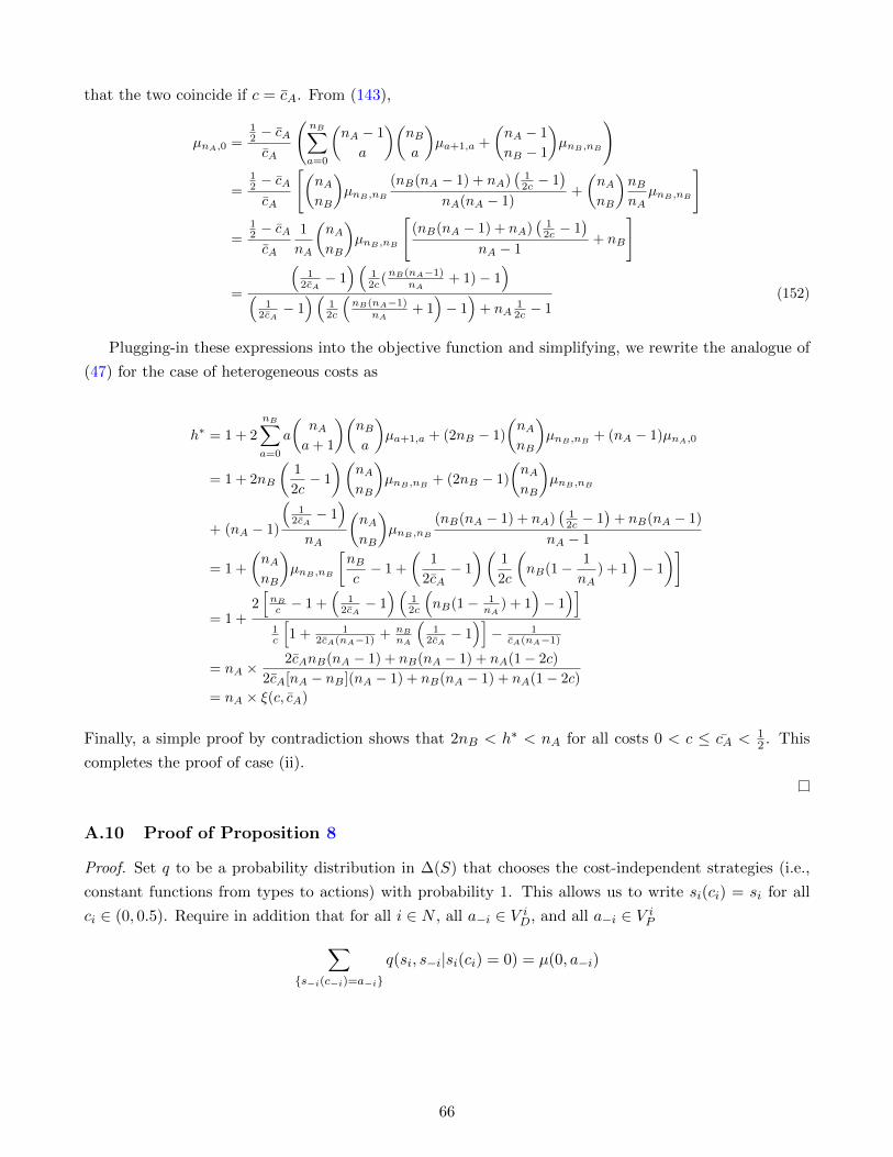
that the two coincide if c = cA. From (143),

µnA,0 =12 − cAcA

(nB∑a=0

(nA − 1

a

)(nBa

)µa+1,a +

(nA − 1

nB − 1

)µnB ,nB

)

=12 − cAcA

[(nAnB

)µnB ,nB

(nB(nA − 1) + nA)(

12c − 1

)nA(nA − 1)

+

(nAnB

)nBnA

µnB ,nB

]

=12 − cAcA

1

nA

(nAnB

)µnB ,nB

[(nB(nA − 1) + nA)

(12c − 1

)nA − 1

+ nB

]

=

(1

2cA− 1)(

12c (nB(nA−1)

nA+ 1)− 1

)(

12cA− 1)(

12c

(nB(nA−1)

nA+ 1)− 1)

+ nA12c − 1

(152)

Plugging-in these expressions into the objective function and simplifying, we rewrite the analogue of

(47) for the case of heterogeneous costs as

h∗ = 1 + 2

nB∑a=0

a

(nAa+ 1

)(nBa

)µa+1,a + (2nB − 1)

(nAnB

)µnB ,nB

+ (nA − 1)µnA,0

= 1 + 2nB

(1

2c− 1

)(nAnB

)µnB ,nB

+ (2nB − 1)

(nAnB

)µnB ,nB

+ (nA − 1)

(1

2cA− 1)

nA

(nAnB

)µnB ,nB

(nB(nA − 1) + nA)(

12c − 1

)+ nB(nA − 1)

nA − 1

= 1 +

(nAnB

)µnB ,nB

[nBc− 1 +

(1

2cA− 1

)(1

2c

(nB(1− 1

nA) + 1

)− 1

)]

= 1 +2[nB

c − 1 +(

12cA− 1)(

12c

(nB(1− 1

nA) + 1

)− 1)]

1c

[1 + 1

2cA(nA−1) + nB

nA

(1

2cA− 1)]− 1

cA(nA−1)

= nA ×2cAnB(nA − 1) + nB(nA − 1) + nA(1− 2c)

2cA[nA − nB ](nA − 1) + nB(nA − 1) + nA(1− 2c)

= nA × ξ(c, cA)

Finally, a simple proof by contradiction shows that 2nB < h∗ < nA for all costs 0 < c ≤ cA < 12 . This

completes the proof of case (ii).


Proof. Set q to be a probability distribution in ∆(S) that chooses the cost-independent strategies (i.e.,

constant functions from types to actions) with probability 1. This allows us to write si(ci) = si for all

ci ∈ (0, 0.5). Require in addition that for all i ∈ N , all a−i ∈ V iD, and all a−i ∈ V i

P∑{s−i(c−i)=a−i}

q(si, s−i|si(ci) = 0) = µ(0, a−i)

66

and ∑{s−i(c−i)=a−i}

q(si, s−i|si(ci) = 1) = µ(1, a−i),

where µ(a) ∈ ∆(S) is the probability distribution over joint action profiles that delivers the solution to

the max turnout problem under complete information with heterogeneous costs defined by C(cA,cA,cB ,cB)

(see Proposition 7). Notice that for cost-independent strategies, the summations on the LHS of the above

expressions are taken over a single strategy. Then for every player i, q selects the constant-zero strategy

si(ci) = 0 ∀ci ∈ (0, 0.5) with probability∑

a−iµ(0, a−i), and the constant-one strategy si(ci) = 1 ∀ci ∈

(0, 0.5) with the complementary probability. Suppose first that cB = cA. Then Proposition 7 holds

at any cost profile c ∈ C(cA,cA,cB ,cB) with the same equilibrium distribution over actions, µ(a) ∈ ∆(S),

because this distribution is completely determined by the cost bounds (cA, cA, cB, cB) and the sizes of the

groups, nA and nB. Therefore, none of the incentive compatibility constraints (38)-(39) is violated at an

arbitrary c ∈ C(cA,cA,cB ,cB). Hence this is true for all admissible c, and both constraints (43)-(44) hold

as well. Therefore, we can guarantee the expected turnout at least as large as h∗. If cB < cA, then, as

discussed in the proof of Proposition 7, the maximum expected turnout exceeds h∗, so again, for any fixed

cost profile c ∈ C(cA,cA,cB ,cB) we can satisfy conditions (38)-(39) with the same equilibrium distribution

µ(a) ∈ ∆(S).


Proof. We start by redefining a SFIICE in the setting with uncertain party sizes. A pure strategy

si : {A,B} × {1, . . . , n− 1} → {0, 1} maps the pair of voter’s type and the realized total size of group A

(note that it may turn out to be a minority group) into a binary action, where 0 stands for abstaining and

1 for voting for the “correct” candidate (thus, we abuse notation and merge together two different pure

actions). Voter types have a common component m, the size of group A, and a private component ti, their

own preference. The set of all pure strategies for player i ∈ N is a finite set Si = {0, 1}{A,B}×{1,...,n−1},

i.e. the set of all functions from type-size pairs into actions. Let S ≡ ×i∈NSi be the set of all joint

strategies. q ∈ ∆(S) is a SFIICE if for all i ∈ N , all (ti,m) ∈ {A,B}× {1, . . . , n− 1}, all ai ∈ {0, 1}, and

any si ∈ Si such that si(ti,m) = ai, we have

n−1∑m=1

PN (m)

∑{t−i|

∑nk=1(1{tk=A})=m}

∑a−i

∑{s−i(t−i,m)=a−i}

q(si, s−i)

[ui(ai, a−i)− ui(a′i, a−i)]

≥ 0 (153)

for all a′i ∈ {0, 1}. Observe that for each realized pair of party sizes, (nA, nB) = (m,n − m) we can

construct a high-turnout correlated equilibrium using Proposition 1, which would have the terms in

the curly brackets in (153) non-negative. Thus, it is sufficient to pick q such that it maps each m ∈{1, . . . , n−1} to a high-turnout correlated equilibrium distribution corresponding to a partition (m,n−m).

Then the entire sum in the incentive compatibility constraints (153) is also non-negative, so all IC

constraints are satisfied, and q is a SFIICE. Since at each m the expected total turnout in this construction

is defined by f∗(m) from Proposition 1, the expected turnout that can be achieved in a SFIICE with

uncertain party sizes is at least EPN(f∗).

67

Correlated Equilibria in Voter Turnout Games

Documents