Correction of Shallow Water Electromagnetic Data for Noise ...

Correction of Shallow Water Electromagnetic Data

for Noise Induced by Instrument Motion

Pamela Lezaeta, Alan D. Chave and Rob L. Evans

Woods Hole Oceanographic Institution, Woods Hole, MA 02543, USA

(December 13, 2004)

Short title: Correction of Electromagnetic Motion Noise

ABSTRACT

An unexpected noise source was found in magnetic and sometimes electric eld

data recorded on the bottom of lakes in the Archean Slave craton (NW Canada) dur-

ing warm seasons. The noise is due to instrument motion and in some instances direct

induction by wind-driven surface gravity waves when the lakes are not ice covered.

The noise can be reduced or eliminated by pre-ltering the data with an adaptive

correlation noise cancelling lter using instrument tilt records, prior to estimation

of magnetotelluric (MT) response functions. Similar eects are to be expected in

other shallow water environments, and the adaptive correlation canceller is a suit-

able method to pre-process MT data to reduce motional noise in the magnetic eld.

This underscores the importance of ancillary tilt measurements in shallow water MT

surveys. In coastal or lake bottom surveys, special eorts to reduce hydrodynamic

eects on the instrument should also be pursued.

INTRODUCTION

During the years 1998-2000, two magnetotelluric (MT) surveys were conducted

on the Archean Slave craton in eighteen lakes over nineteen deployments using con-

tinental shelf electromagnetic instrumentation designed for use at depths lower than

1

1000 m (Pettit et al., 1994). The instruments were deployed from oat airplanes dur-

ing the ice-free summer months and retrieved in the subsequent summer. The rst

sequence of lakes was surveyed for eleven months, at which point the instruments were

retrieved and transferred to a second series of lakes for another year. The measure-

ments were aimed at determining the regional-scale three-dimensional (3-D) electrical

structure of the craton (Jones et al., 2003). During the rst month of each survey, the

data were recorded at a high sample rate (1.75 s) for imaging crustal features. The

instruments then switched automatically to a lower sample rate (28 s) for the remain-

der of the deployment to obtain long period MT data, permitting deep penetration

into the lithospheric mantle and below. Each instrument was programmed to record

the time variations of the two orthogonal horizontal electric elds across a 3 m span

using Ag-AgCl electrodes, and the three-component magnetic eld variations were

measured using a suspended magnet sensor (Filloux, 1987). The horizontal plane

tilt variations of the cylindrically shaped magnetometer pressure case were also mea-

sured with microradian resolution. Figure 1 shows a picture of an instrument being

deployed. Instrument installation depths ranged from 7 to 50 m, with 15-20 m being a

typical value. Time series of tilt and magnetic eld were stable in wintertime except

for normal geomagnetic variations, while they displayed strongly disturbed intervals

from late spring through summer and into early fall. The disturbance was particularly

noticeable in the high sample rate data, where short period tilt variability correlated

strongly with the magnetic eld (and sometimes the electric eld) uctuations. Such

noise was somewhat unexpected, as the lakes were expected to be calm with weak

water currents in comparison to the continental shelves.

This paper focuses on the analysis of nonstationary instrument motion that af-

fected the magnetic (and sometimes the electric) eld data, and on the development

of a time-domain mitigation technique for the correlated noise using an adaptive

correlation cancellation lter prior to estimation of frequency-domain MT response

functions. We also propose a physical explanation for the cause of the instrument

2

motion and suggest a possible means to minimize the problem.

DATA SET

Figure 2 shows the location of the lake bottom sites. In the rst survey, from Au-

gust 1998 to August 1999, ten sites were recorded, and nine more sites were occupied

in the second year, from September 1999 to August 2000.

The electric and magnetic channels were edited to correct for obvious instrument ef-

fects (such as infrequent data spikes and regular magnetic eld calibration pulses) and

high pass ltered to remove long term drift using a fourth order Butterworth lter

having a 24,000 s cuto period run forward and backward across the data to elimi-

nate possible phase shifts. Due to inevitable and uncontrollable electrode drift, the

two electric channels occasionally were out of range even with gain ranging applied,

producing some data gaps in one or both components. The magnetic time series were

continuous. Figure 3 shows examples of magnetic and electric time variations from

Newbigging Lake (site newBig in Fig. 2) for a 10 h window at the high (1.75 s) sam-

ple rate. During the rst six hours, the data have a higher frequency character than

during subsequent hours, particularly for the magnetic eld. The magnetic eld and

tilt variations approximately covary during the rst six hours of the window (Fig.4).

Many sites displayed similar correlations in the high sample rate time series during

the summer months.

TILT NOISE CORRELATION WITH FIELD COMPONENTS

The corresponding components of tilt and magnetic eld vary coherently when

the high frequency disturbance is present. This disturbance was generally at least

twice as large for the component (Y) across the magnetometer cylinder compared

to the along-cylinder (X) component. Although not truly periodic, the variations

have a dominant period of about 4.5 sec which becomes clear for short time windows

3

(Fig.5). The electric eld (E) is usually not correlated with the disturbed tilt except

in extreme cases. Figure 6 shows an example for the Y component from Newbigging

Lake, while the Ex eld seems unaected by the tilt motion (Fig.6; top). The electric

eld perturbation when present lasted from a few minutes to as long as several hours,

also with a period of ∼4.5 s.

It is well known that mechanical motion of a magnetometer in Earth's magnetic eld

will generate an apparent magnetic eld (e.g., Bastani and Pedersen, 1997), and hence

correlated noise, but this should not aect the electric eld unless vxB is comparable

to the ambient eld (Eq.6) and there is local induction in the surrounding medium,

as occurs in the highly conductive ocean for a variety of water disturbances. Further

discussion is presented in a later section.

Power spectra for the magnetic eld and tilt computed from perturbed and quiet

time segments (Fig.7) show that tilt motion systematically aected the magnetic eld

at periods below 1000 s, with peak amplitudes centered below 10 s (Fig.7), consistent

with the time series plots. During disturbed times, the high frequency magnetic eld

noise oor rises by up to four decades in power, consistent with the change for tilt.

The tilt motion also systematically aected the vertical magnetic eld component

by around one to two decades in power, while it was not signicant in the power

spectrum of the electric eld components for the majority of the sites.

NOISE REMOVAL WITH AN ADAPTIVE CORRELATION

CANCELLATION FILTER

The tilt-induced noise is highly variable in time, and hence removal using

frequency-domain transfer function methods implicitly dependent on the stationarity

assumption are of little use. Time-domain data adaptive ltering methods have been

developed that are applicable to non-stationary situations, of which the most useful in

4

the present context is the adaptive correlation canceller (Widrow and Stearns, 1994).

The adaptive correlation canceller incorporates time-variable lter coecients which

change in an optimal sense to remove unknown interference contained in a primary

signal, using a noise reference in which the primary signal is weak or nonexistent

(Fig.8). In the present case, the primary, contaminated signal is a component of the

magnetic (or sometimes, electric) eld and the reference (noise) signals are the two

horizontal components of tilt. Each adaptive lter is a linear transversal (nite im-

pulse response) lter whose coecients are updated at each time step using the least

mean square (LMS) algorithm.

Let the primary signal be given by:

S = So + no , (1)

where no represents the noise in S that is correlated in an unknown manner with the

corrupted signals or reference noise Ref1 and Ref2 (i.e., the two tilt components).

The signal free of such noise is thus given by So.

At the discrete time m, let the predicted noise y(m) be the sum of the outputs of the

adaptive lters, let the adaptive lter coecients be W1(m) and W2(m), and let the

reference signals be Ref1(m) and Ref2(m) (Fig.8). Then, the output of the adaptive

lter at time m is

y(m) = W1(m) · Ref1(m) + W2(m) · Ref2(m) = W(m) ·Ref(m) (2)

Using the LMS algorithm, at time step m+1, the lter (W in equation 2) is given by:

W(m + 1) = W(m) +µ · err(m) ·Ref(m)t

α +∑N

i=1 Ref(m− i)2 (3)

with t representing the transpose of Ref and N the lter length. The coecient µ

(equation 3) is the adaption step size of the time domain lter and α is a damping

factor, both of which are found iteratively by minimizing the sum of squared dier-

ences between the input data and the predicted noise (err2(m); equation 4) over the

5

time space of input data m (m=1,..,Nd; number of data). The output signal at the

discrete time m is the dierence between the primary input signal X_in delayed by

a given time (N/2) and the lter output signal y(m):

err(m) = X_in(m− N/2)− y(m) , (4)

where N/2 is a delay time introduced to "grow" the coecients toward the center

of the lter (W; equation 3), so that if timing between the input primary signal

X_in(m) and the reference noise (Ref) is not aligned, the correlator W will be able

to nd the correct value (within the interval ±N/2 of the lter length N). The starting

set of adaptive lters W(m) (i.e., for m=1,..,N) are initialized to zero at a rst step

(each step is over the time space Nd of input data), so that for further steps, W will

start from the previous result, computing the following W(m) as in equation 3 to get

the output err(m) (equation 4) from the sum of predicted noise (eq.2) over the lter

length (N):

y(m) =∑N

i=1(W(m− i)Ref(m− i)) (5)

When the variance of err (Nd∑

m=1

err(m)2

Nd−1) has changed minimally from the previous step,

then the nal err(m) is considered to be the clean output X_out(m) (ideally So;

equation 1) at the discrete time m. Because of the large dynamic range of the time

series, better performance is typically achieved by rst prewhitening each time series

using a robust autoregressive (AR) lter (Chave and Thomson, 2004).

The application of the noise canceller to the Slave lakes data gave, in general,

satisfactory results. Figure 9 shows segments of noise-cancelled magnetic eld signals

along with the original (prewhitened) disturbed time series from Lake Tete d'Ours

from the rst year survey. Tilt amplitudes (also prewhitened with the AR lter) for

this site varied by up to 200 microradians in the time interval selected (from 13th

to 15th of August). The electric eld within this interval was not aected by tilt,

suggesting purely mechanical (non-inductive) noise on the magnetic channels.

6

The noise canceller did not always fully succeed on magnetic time series having

extreme disturbance levels, which usually occurred when the electric eld channels

were also aected by tilt. Figure 10 shows such magnetic and electric time series

from Aylmer Lake. This site was the shallowest deployment of the survey at 6 m,

and both tilt components have similar amplitudes of up to 250 microradians. The

adaptive correlation lter achieved only a partial reduction in the peak time series

amplitude, thus reecting limited cancellation of the tilt-induced noise. Electric and

magnetic eld power spectra of noise-cancelled peak segments demonstrate this, with

values one to two orders of magnitude above the spectrum from a quiet segment (not

shown).

After noise cancellation, the MT and magnetic transfer functions were estimated

using the bounded inuence remote reference algorithm of Chave & Thomson (2004).

This algorithm eliminates highly disturbed segments automatically provided there is

minimal correlation between the corresponding electric (E) and magnetic (B) eld

components. Low correlation occurred when the B eld was aected by tilt, therefore

MT impedances (the ratio of E to B eld) estimated from time-series after applying

the noise-canceller showed generally small improvements over the estimates without

application of the lter, with the only notable dierences at the shortest periods

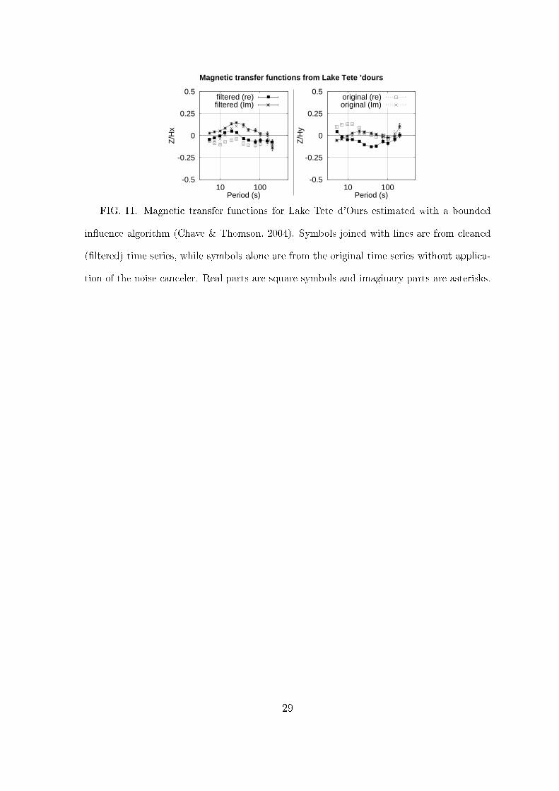
(<20 s; not shown). Figure 11 shows the magnetic transfer responses (the ratio of

vertical- to horizontal-component of the B eld) for Lake Tete d'Ours estimated from

the original and the cleaned time series, showing dierences between both curves

even at periods over 10 s. In addition, the use of two stage processing with a clean

remote reference site to remove correlated noise from the input (magnetic eld) time

series prior to estimation of the transfer functions (Chave and Thomson, 2004) was

needed to further reduce the bias at the shortest periods, and for matching the curves

obtained between the responses from the high and low sampling rate data in the

period range of 100 s to 1000 s.

7

TILT AND WIND CORRELATION: EFFECT OF WIND WAVES

The Canadian Meteorological Service maintains four weather stations located in

the western sector of the MT array where most of the sites from the rst year survey

are located. While the correlation scale of wind is typically a few meters, and hence

a statistical correlation of the wind from a distant station with local tilt is not likely,

correlation of intervals of high wind with large tilt variations does suggest a causative

relation. Further, such a relation is suggested by the occurrence of disturbed tilt

intervals during the warm months when the lakes are not frozen, and hence subject

to the generation of wind waves.

We analyzed the summer and early fall months of August, 1998 and Septem-

ber, 1999, respectively, which are the times when the high sampling rate data from

the two year-long surveys were recorded. During August 1998, the average wind di-

rection at each weather station when the wind speed was over 15 km/h is spatially

homogeneous and points from the SSW, with mean values ranging from 23 to 27 km/h.

In September 1999, the wind direction was more to the north (i.e., a southerly wind)

with average wind speed very similar to that from August of the previous year.

Highly disturbed tilt events consistently coincide with high wind. This indicates

that the wind is a driving force (direct or indirect) for water movements at the bottom

of the lakes where the MT instruments are located. The highly disturbed segments

with the largest tilt amplitude occurred when wind speeds were extremely high (usu-

ally with values exceeding 30 km/h), even for sites set beyond 20 m depth. Usually

a time delay of a few hours is observed between peak wind and peak tilt. Peak

winds (up to 55 km/h) typically last for about 3 h, followed by a calmer interval

of a few hours before high winds recur. However, tilt continues to be consistently

disturbed despite the sequence of low and high wind speeds, usually lasting for up

to two to three days (see data from Lake Tete d'Ours in Figure 12). Intuitively,

instrument motion and/or local induction by wind-driven surface gravity waves are

8

the most likely mechanisms for the observed tilt disturbance. Proving this would re-

quire data and models which are not readily available, notably wind data distributed

around each lake, depth information about the lakes, and measurements of the elec-

trical conductivity of lake water. It would also require a sophisticated model of the

mechanical response of the lake bottom instruments to water motion over a range

of spatial scales and frequencies. None of these are available, and hence recourse

to simple bounds on the water motion produced by wind-induced waves and on the

response of a cylindrical body to wave motion will be made.

Gravity wave response to wind forcing occurs over a continuum of frequencies,

depending strongly on the fetch and water depth and on the wind growth. Wave

prediction models are available for coastal areas which can be restricted in depth and

laterally based on nite water depth linear theory (Automated Coastal Engineering

System ACES 7B; http://www.veritechinc.com/navigate.htm), though these are only

approximately applicable to the more tightly bounded geometry of the Slave lakes.

Assuming wind speeds between 25 and 37 km/hr lasting for three hours or longer

(Fig.12), estimates of wave periods and wave amplitudes were obtained from this

algorithm for combinations of input variables. The dominant variables were fetch

(from 2 to 30 km) and lake depth (10 to 50 m), and of secondary importance the

dierential temperature between the air and water interface (a few degrees). Wave

periods between 1-2 s and amplitudes of 0.2-0.4 m for the smallest lakes (fetch <7 km)

and around 3-5 s period and 0.4-0.6 m amplitude for the largest Slave lakes (fetch of

10-20 km) were obtained.

Wave angular frequency (ω) and wavenumber (k) for surface gravity waves are

related through the nite water depth dispersion relation: w2 = g k tanh(kd), where

g is the acceleration of gravity and d is the water depth. At a wave period of 4.5 s and

a water depth of 20 m, the wavenumber is 0.19887, so that the wavelength is 31.6 m.

The deep water approximation is obtained when kd > π, so that w2 ∼ gk, implying

that deep water theory is appropriate for the lakes, assuming maximum wave periods

9

of about 5 s if wind growth is the dominant force for surface gravity wave generation

during high wind events. At a short wave period of 1 s (more likely at the smaller

lakes) and water depth of 10 m, the wavelength is 2 m and hence the deep water

approximation becomes even more valid. At longer wave periods, deep water theory

does not apply.

The deep water motion (orbital velocity v) from surface gravity waves decays

exponentially with depth (z) according to v = ω A e−kz, where A is the surface wave

amplitude. Assuming a wave period of 3 s at an amplitude of 0.6 m, the horizontal

water particle displacement is 1.2x10−8 cm/s on a lake bed of 50 m depth (the deepest

instrument deployment), 0.0074 cm/s at 20 m depth (the general instrument depth),

and 4 cm/s at 6 m depth (the shallowest deployment). Hence surface gravity wave

induced instrument motion may well account for the tilt oscillations.

Further insight can be obtained from the observation that the tilt motion is typ-

ically 3-4 times larger across the magnetometer cylinder (Y-axis) compared to along

the cylinder (X-axis). This is consistent with the higher force needed to lift the larger

cross-sectional area along X than is needed for lifting (or rotating in this case) along

its cylinder diameter (Y). Karman vortex shedding of the magnetometer cylinder can

be estimated from the nondimensional Strouhal number S, which is typically 0.22

in laminar ows (e.g., Newman, 1997). S is the product of vortex frequency and

cylinder diameter divided by water velocity. At a dominant period of 4.5 s and for a

cylinder diameter of 23 cm, the water velocity would have to be 23 cm/s to produce

S ∼ 0.22. This is much higher than the velocities estimated for surface gravity waves,

and also higher than any other likely disturbance. For example, internal waves for

typical stratied lakes have estimated velocities between 1 and 10 cm/s at the lake

bed (Nepf, pers. comm., 2003). Unless the instrument is excited in one of the modes

of its natural resonance frequency by the water mass passing by the cylinder, vortex

shedding does not appear to be an explanation for the observed tilt.

Finally, we note that there are two sites which never displayed large summer-time

10

tilt variations: Duncan and Kuuvik. The former is located close to Yellowknife where

the wind speed was lower than at northern locations. Further, its fetch is negligible

under the direction of strong wind measured at that time, suggesting that surface

wave generation is weak. An explanation for the behavior of the very small Lake

Kuuvik is lacking.

MOTIONAL ELECTRIC FIELD FROM SURFACE GRAVITY WAVES

We have shown in a previous section that some sites displayed electric as well as

magnetic eld variations correlated with tilt (Fig.10), hence suggesting electromag-

netic induction by water motion.

The electric eld amplitude induced by a moving medium (water in this case) is

given by Ohm's law:

E′ = E + v ×B (6)

(e.g., Larsen, 1971), where E′ is the electric eld in a reference frame moving at

velocity v, E is the E eld in a xed reference frame, and B is the steady geomagnetic

eld. This provides the basic principle for estimation of motion-induced electric

and magnetic elds within the ocean and lakes. The equation for the electric and

magnetic elds induced by a plane progressive gravity wave in a at-bottomed water

body of uniform depth has been estimated by diverse authors (e.g., Weaver, 1965;

Larsen, 1971). Assuming the thickness of the conductive water layer, sedimentary

cover, and the lithosphere to be small compared to the wavelength of the incident eld,

and a negligible conductivity for the air and the lithosphere (underlain by a conductive

mantle), Larsen (1971) derived the motional electric eld induced by surface gravity

waves. Assuming the Slave lakes may be approximated by a model with a uniform

water depth and an innite lateral extent like the ocean, the motional horizontal

electric and vertical magnetic elds can be estimated by using the formula derived by

11

Larsen (1971; Eqs.17 and 23). If we consider fresh water conductivity to range from

0.1 to 0.01 Ω−1m−1, subject to wind waves of period up to 5 s and wave amplitude up

to 0.8 m, with uniform water depth ranging from 7 to 10 m, the horizontal electric eld

reaches a magnitude of around 0.2 mV/km and the vertical magnetic eld amplitude

is up to 0.01 nT. These estimates cannot explain the eect of electric eld noise

observed in the instruments deployed at 6 m depth in the large Aylmer Lake and

at 10 m depth in the small Newbigging Lake, where the dierences between a calm

and a disturbed E eld were on the order of 10-15 mV/km for Aylmer Lake and

∼8 mV/km for Newbigging. This suggests that the approach of a at bottom for

the Slave lakes is not appropriate and/or the water motion in these lake beds is not

caused solely by surface gravity waves from wind driven forces. Considering wave

periods beyond 5 s would cause the breakdown of Larsen's (or Weaver) equations,

as these are based on intermediate and deep water wave theory, which are limited

by the depth of the deployment (10 m) in this case. Considering E eld amplitudes

generated directly from the instrument motion, a simple calculation shows that the

electrodes must move at improbably high speeds (|v|) of around 20 cm/s for vxB

(Eq.6) to be comparable to the E eld disturbance observed. Such a speed is similar

to the laminar ow velocity estimated from vortex shedding of the magnetometer.

Is that a mere coincidence or is it because the instrument oscillated at some natural

resonance frequency mode by the water motion? To answer this question will require

data not available at present.

SUMMARY AND DISCUSSION

We have shown, from magnetotelluric (MT) surveys performed on the bottom of

lakes of the Slave craton (NW Canada), that magnetic eld data were disturbed by

instrument motion that also registered in measurements of tilt. In some cases the

electric eld may also have been aected by electromagnetic induction generated by

12

water motion.

The disturbances in the time series were highly correlated with tilt with a relatively

consistent dominant period of around 4 s, regardless of the depth and size of the lakes

where the instruments were deployed. The magnetic and sometimes electric eld

channels can be pre-treated with an adaptive correlation cancellation lter using the

two components of tilt as a reference signal. The method satisfactorily reduces the

noise in the electromagnetic data under most circumstances. Exception are seen

for some sites where the electric eld noise was not negligible and hence there is

correlated noise in the electric and magnetic channels. In this case, information on

rotation of the instrument about the local vertical may be needed for an optimal noise

cancellation. In addition, a two stage bounded inuence processing algorithm with a

clean remote reference site was generally required for processing of the ltered time

series to obtain stable MT responses.

In order to reduce the instrument motion, it would be desirable to install the

magnetometer in a solid package with a geometry that minimizes vortex shedding and

thereby limits the oscillatory forces on it. In general, this means placing instruments

close to the bottom with a minimum of buoyancy and the center of buoyancy located

close to the center of mass of the anchor. In addition, a spherical case with small

dimples like a golf ball can help reduce vorticity, although at the cost of increased

drag force. Reduction of drag force upon the instrument can be achieved using a

stier and heavier base (a rigid tripod of ∼25 kg was used in this survey). These

considerations are of particular importance in coastal regions where sea bed currents

are expected to be strong, for which tilt-induced electromagnetic elds from the water

movement could be signicant.

13

ACKNOWLEDGEMENT

We would like to thank the Canadian Meteorological Service for providing the wind

data, and Alan G Jones, Xavier Garcia, Jessica Spratt, Helmut Moeller, Jonathan

Ware and John Bailey for their assistance in eld work and in the data analysis. The

advice given by Heidi Nepf (MIT) and Mark Grosenbaugh (WHOI) were valuable

for gaining insight into the possible physical explanations for the instrument mo-

tion. Thanks also to Todd Gregory for useful suggestions to improve the manuscript.

Commentaries given by the reviewers helped to improve the clarity of the manuscript,

especially the review by L. Pedersen.

This project was funded by NSF grant EAR-9725556 and EAR-0087699. P.L. ac-

knowledges the Fundacion Andes for a postdoctoral grant.

REFERENCES

Bastani, M., and L.B. Pedersen, The reliability of aeroplane attitude determination

using the main geomagnetic eld with application to tensor VLF data analysis,

Geophysical Prospecting, 45, 831-841, 1997.

Chave, A.D., and D.J. Thomson, Bounded inuence estimation of magnetotelluric

response functions, Geophys. J. Int., 157, 988-1006, 2004.

Jones, A.G., P. Lezaeta, I.J. Ferguson, A.D. Chave b, R.L. Evans, X. Garcia &

J. Pratt, The electrical structure of the Slave craton, Lithos, 71, 505-527, 2003.

Larsen, J.C., The electromagnetic eld of long and intermediate water waves, J. Mar.

Res., 29, 28-45, 1971.

Newman, J.N., Marine Hydrodynamics, The MIT Press., Cambridge, Massachussets,

pp.402, 1997.

14

Petitt, R.A., Jr., Chave, A.D., Filloux, J.H., and Moeller, H.H., Electromagnetic eld

instrument for the continental shelf: Sea Technology, 35, 10-13, 1994.

Weaver, J.T., Magnetic variations associated with ocean waves and swell, J. Geophys.

Res., 70, N.8, 1921-1929, 1965.

Widrow, B. and Stearns, S.D., Adaptive Signal Processing, Prentice-Hall, Inc., En-

glewoods Cli, New Jersey, 1985.

15

FIG. 1. A seaoor instrument used in the lake bottom surveys on the Slave craton being

deployed from a twin Otter oatplane. Arrows indicate the parts of the instrument; the

electrodes (at the ends of the two orthogonal light plastic pipes) are above the magnetometer

and tilt sensor inside a horizontal cylindrical aluminum pressure case. Tilt is the angular

deection of the two horizontal principal coordinates of the cylinder, and are rotated by 45Æ

from the horizontal electrode pipes. The tripod anchor for the instrument is underwater.

19

FIG. 2. Location of MT stations deployed on the bottom of lakes in the Slave craton

(NW Canada). Black dots and triangles are sites from the rst and second year surveys,

respectively. YK : Weather station Yellowknife. Inset above shows a regional map of Canada.

20

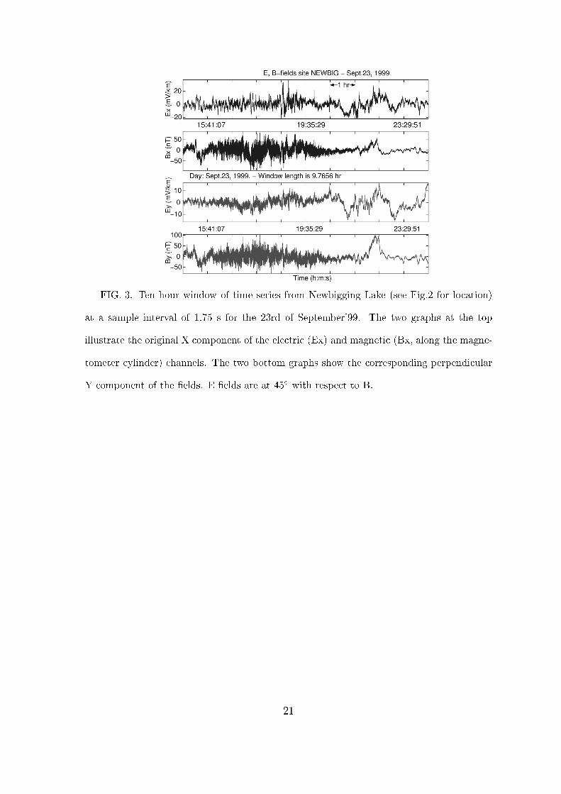
FIG. 3. Ten hour window of time series from Newbigging Lake (see Fig.2 for location)

at a sample interval of 1.75 s for the 23rd of September'99. The two graphs at the top

illustrate the original X component of the electric (Ex) and magnetic (Bx, along the magne-

tometer cylinder) channels. The two bottom graphs show the corresponding perpendicular

Y component of the elds. E elds are at 45Æ with respect to B.

21

FIG. 4. Ten hour window of magnetic eld and tilt variations from Newbigging Lake

(see Fig.2 for location) at a sample interval of 1.75 s for the 23rd of September'99. The four

traces from top to bottom illustrate the horizontal X component of the magnetic eld (Bx)

and tilt (Tilt-x) and the Y component By and Tilt-y, respectively. Tilt is in microradians.

The horizontal components are as for Figure 3.

22

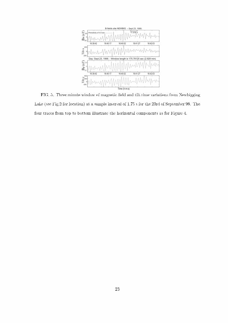
FIG. 5. Three minute window of magnetic eld and tilt time variations from Newbigging

Lake (see Fig.2 for location) at a sample interval of 1.75 s for the 23rd of September'99. The

four traces from top to bottom illustrate the horizontal components as for Figure 4.

23

FIG. 6. Three minute window of the electric eld (in the measurement coordinate sys-

tem) and tilt time variations from Newbigging Lake (see Fig.2 for location) at a sample

interval of 1.75 s for the 23rd of September'99. The four traces from top to bottom illus-

trate the horizontal components as for Figure 4.

24

FIG. 7. Power spectra as a function of period for the magnetic elds components Bx and

By (left) and the tilt components X and Y (right) for Lake Tete d'Ours. The two curves

in each plot correspond to the power spectrum from highly disturbed (dists; 11-12 Aug'98)

and relatively quiet tilt time segments (7-10 Aug'98).

25

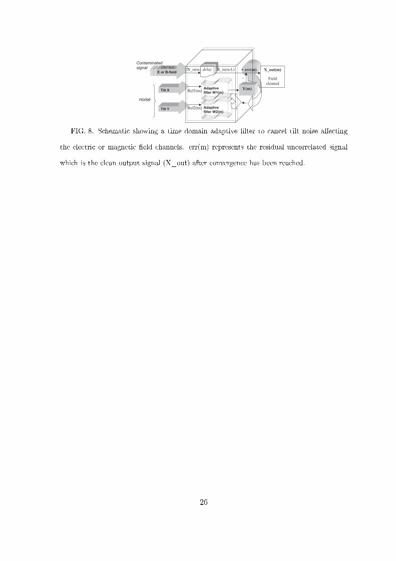
FIG. 8. Schematic showing a time domain adaptive lter to cancel tilt noise aecting

the electric or magnetic eld channels. err(m) represents the residual uncorrelated signal

which is the clean output signal (X_out) after convergence has been reached.

26

FIG. 9. Prewhitened time series of original (dark curve) and noise-cancelled horizontal

components (in gray) for Lake Tete d'Ours in the measurement coordinate system. Curves

from top and bottom are the magnetic Bx and By components at 106Æ and 196Æ from

geographic north, respectively. The time window is during summer between the 13th and

15th of August, 1998.

27

FIG. 10. Prewhitened time series of original (dark curve) and noise-cancelled horizontal

components (in gray) for Aylmer Lake in the measurement coordinate system. Graphs from

top and bottom are both the electric (Ex) and the magnetic (By) components at 185Æ and

230Æ from geographic north, respectively. The time window is during fall between the 19th

and 26th of September, 1999.

28

-0.5

-0.25

0

0.25

0.5

10 100

Z/H

x

Period (s)

filtered (re)filtered (Im)

-0.5

-0.25

0

0.25

0.5

10 100

Z/H

y

Period (s)

original (re)original (Im)

Magnetic transfer functions from Lake Tete ’dours

FIG. 11. Magnetic transfer functions for Lake Tete d'Ours estimated with a bounded

inuence algorithm (Chave & Thomson, 2004). Symbols joined with lines are from cleaned

(ltered) time series, while symbols alone are from the original time series without applica-

tion of the noise canceler. Real parts are square symbols and imaginary parts are asterisks.

29

FIG. 12. Top: Hourly wind speeds at Yellowknife during August'98 and bottom the

two components of prewhitened tilt (microradians) from Lake Tete d'Ours recorded during

that same month. Ovals denote correlation between wind peaks and highly disturbed tilt.

Location of the sites are shown in Figure 2.

30