Corporate Default with Chinese Characteristics Jing Ai & , Warren Bailey*, Haoyu Gao $ , Xiaoguang Yang, and Lin Zhao # 19th April 2017 Abstract We study lending, default, and default resolution with seven million loans by seventeen commercial banks to corporations across China from 2007 to 2013. Politically-connected borrowers are more likely to default, particularly with an underdeveloped headquarters region or government-controlled lender. With bankruptcy law improvements or fiscal stimulus, these borrowers are relatively more likely to default and resolve default quickly. Once listed on a stock market, they are relatively more likely to borrow more and resolve default slowly. However, evidence of relationship banking and improvements in some lending outcomes after listing suggest the gradual emergence of a modern capital market. Keywords: bank loans, relationship banking, corporate default, government bailout, China, politically-connected firms, state-owned enterprises JEL Classifications: G21, G28, G33, G38 * Corresponding author: Johnson Graduate School of Management, Cornell University, 387 Sage Hall, Ithaca, NY 14853, USA, [email protected]. & Shidler College of Business, University of Hawai'i at Manoa, 2404 Maile Way Honolulu, HI 96822, USA, [email protected]. $ Chinese Academy of Finance and Development, Central University of Finance and Economics, No. 39, Xueyuan South Road, Beijing, China, 100081, [email protected] # Academy of Mathematics and Systems Science, Chinese Academy of Sciences, Beijing, 100190, PRC, [email protected], and [email protected]. We thank the Chinese Bank Regulatory Commission for access to its unique database of loan defaults and other information without which this study would not be possible. We thank participants at Moody’s Corporation and Shanghai Advanced Institute of Finance “The First Annual Credit Market Research Conference in China” (2014), the Chinese International Conference of Finance (Chengdu, 2014), Colorado State University, Chinese University of Hong Kong, Hong Kong Polytechnic University, Nanyang Business School, Bank for International Settlements (Hong Kong), Columbia University’s Fourth Symposium on Emerging Financial Markets: China and Beyond, May 2015, Xiamen University, University of Hong Kong, University of Western Ontario, and Michael King, Hong Zhang, and Murillo Campello in particular for comments, helpful discussions, or other assistance. © 2014, 2015, 2016, 2017, Jing Ai, Warren Bailey, Haoyu Ga, Xiaoguang Yang, and Lin Zhao

Welcome message from author
This document is posted to help you gain knowledge. Please leave a comment to let me know what you think about it! Share it to your friends and learn new things together.
Transcript
Corporate Default with Chinese Characteristics
Jing Ai&, Warren Bailey*, Haoyu Gao$, Xiaoguang Yang, and Lin Zhao#
19th April 2017
Abstract
We study lending, default, and default resolution with seven million loans by seventeen commercial banks to corporations across China from 2007 to 2013. Politically-connected borrowers are more likely to default, particularly with an underdeveloped headquarters region or government-controlled lender. With bankruptcy law improvements or fiscal stimulus, these borrowers are relatively more likely to default and resolve default quickly. Once listed on a stock market, they are relatively more likely to borrow more and resolve default slowly. However, evidence of relationship banking and improvements in some lending outcomes after listing suggest the gradual emergence of a modern capital market.
Keywords: bank loans, relationship banking, corporate default, government bailout, China, politically-connected firms, state-owned enterprises
JEL Classifications: G21, G28, G33, G38
* Corresponding author: Johnson Graduate School of Management, Cornell University, 387 SageHall, Ithaca, NY 14853, USA, [email protected]. & Shidler College of Business, University of Hawai'i at Manoa, 2404 Maile Way Honolulu, HI 96822, USA, [email protected]. $ Chinese Academy of Finance and Development, Central University of Finance and Economics, No. 39, Xueyuan South Road, Beijing, China, 100081, [email protected] # Academy of Mathematics and Systems Science, Chinese Academy of Sciences, Beijing, 100190, PRC, [email protected], and [email protected]. We thank the Chinese Bank Regulatory Commission for access to its unique database of loan defaults and other information without which this study would not be possible. We thank participants at Moody’s Corporation and Shanghai Advanced Institute of Finance “The First Annual Credit Market Research Conference in China” (2014), the Chinese International Conference of Finance (Chengdu, 2014), Colorado State University, Chinese University of Hong Kong, Hong Kong Polytechnic University, Nanyang Business School, Bank for International Settlements (Hong Kong), Columbia University’s Fourth Symposium on Emerging Financial Markets: China and Beyond, May 2015, Xiamen University, University of Hong Kong, University of Western Ontario, and Michael King, Hong Zhang, and Murillo Campello in particular for comments, helpful discussions, or other assistance.
© 2014, 2015, 2016, 2017, Jing Ai, Warren Bailey, Haoyu Ga, Xiaoguang Yang, and Lin Zhao
1
1. Introduction
Creative destruction is a key feature of a modern, market-oriented economy. Ideally,
markets for goods and services, labor, talent, and capital punish failure and reward success,
thereby offering better products to consumers, better inputs to companies, and appropriate
rewards to investors. Limited liability corporations, leverage, and the possibility of distress,
default, and bankruptcy contribute to this process. Formal and informal mechanisms to resolve
default are intended to obtain money to meet obligations to creditors, keep a fundamentally
healthy business operating, or, if necessary, liquidate the assets of a firm that cannot be
reorganized profitably. The threat of distress gives managers and shareholders incentives to use
the firm’s assets optimally, thereby reducing the potential for default.
We study corporate borrowing, default, and the resolution of default in China, a novel,
important, but rarely-studied setting with which to examine the workings of a financial system.
We uncover generic lessons about banking and corporate finance from the laws, regulations,
institutions, and practices arising from China’s recent history of very rapid political and
economic change. Along with high economic growth, China continues to experience the
development of modern financial institutions, improvements to the laws and regulations that
govern economic activity, repeated reforms to state-owned enterprises and the banking system,
and looming problems signaled by recent bond defaults. A significant amount of variability in
the quality of institutions and economic growth across provinces makes China particularly
interesting, as does the presence of both state-directed and more commercially-oriented lenders.
“The China Model” or “The Beijing Consensus” is a subject of great interest to policy-makers
and academics in both developing and developed countries given China’s recent high growth and
the contrast to typical Western political and economic systems.
We focus on what happens when a corporate borrower in China becomes distressed and
misses a payment on a bank loan. There is very little empirical evidence or even descriptive
writing on corporate distress in China. In a survey of the efficiency of the formal bankruptcy
process across 88 countries, Djankov, Hart, McLiesh, and Shleifer (2008) report only limited
information on the foreclosure process in China, and do not report any information on
reorganization or liquidation, perhaps because of the uncertainty and lack of precedents as
2
China’s legal system evolves away from that appropriate to a centrally-planned economy.1
Private resolution of corporate default seems sensible given the state of the legal system in China.
As described below, the resolution of corporate default in China is largely conducted out of court.
While the literature on corporate default confirms the value of informal approaches, other aspects
of Chinese capital markets and political economy can dilute or even reverse the benefits of
private reorganization. In a study of European companies, Borisova and Megginson (2011) find
that government-owned firms enjoy reduced ex ante borrowing costs, suggesting either implicit
or explicit government guarantees. For China in particular, Bailey, Huang, and Yang (2011)
find evidence consistent with the use of loans from the largely state-controlled banking sector to
support weak firms. There is also limited evidence that some dimensions of banking in China
reflect relationships between banks and borrowers and among firms.2
In the financial systems of many developing countries like China and more than a few
developed countries, banks are not merely one component of the capital market but are the
central or exclusive institutions. Bank lending is the traditional channel for Chinese firms to
obtain external financing although some small and medium sized firms also rely on informal
financing (Allen, Qian, and Qian, 2005) and continues to predominate.3 Relationships have
traditionally been a key component of Chinese business culture. In addition to the privately
formed relationships between the banks and the borrowing firms through repeated or long-term
business transactions (Boot, 2000), political connections serve as a special type of relationship
and can influence credit decisions and the default rate of granted loans. As China's economy has
grown and evolved, banks have come under great political pressure to meet competing goals of
supporting social stability while transforming themselves into modern financial institutions
(Dobson and Kashyap, 2006). Furthermore, the Chinese government has encouraged forming
business groups to further economic development, perhaps due to their successful use in 1 Fan, Huang, and Zhu (2013) infer distress from z-scores and information in annual reports for listed Chinese companies. They find that the quality of local government institutions and extent of private ownership relate to successful recovery. 2 Using a proprietary database from a single credit guarantee firm in China, Dybvig, Shan, and Tang (2012) distinguish the risk assessments and collateral-related motivations of lenders versus third-party guarantors. Using a proprietary database from a single Chinese state-owned bank, Chang, Liao, Yu, and Ni (2014) find that “soft” (relationship) information has high predictability for loan default. Using detailed loan records from a Chinese state-owned bank, Qian, Strahan, and Yang (2015) study the effect of delegating loan decisions from committees to individual loan officers. Ru (2015) studies the impact of loans from one of China’s policy banks, China Development Bank, on SOE borrowers, competing firms, and complementary firms. 3 Banks’ share of new credit is about sixty percent. See “Dark and Stormy”, The Economist 7th May 2016.
3
neighboring Japan and Korea. The size, importance, rapid evolution, and unique characteristics
of the Chinese economy warrant a comprehensive look at associations between loan defaults,
banking practices, relationships among banks, firms, and business groups, and government
intervention.
While China’s capital market remains centered on bank debt rather than public bond
issues, defaults on corporate bonds are growing as the Chinese economy matures and raise
questions about the process of default and its resolution. Recent credit events involving Chinese
corporate bonds have received much attention. Suntech Power Holdings, once the world’s largest
producer of solar panels, defaulted on over half a billion dollars in bonds due to be repaid in
March 2013. Court actions were launched in the US where the bonds and common stock of the
firm trade. The default also breached terms of other debt including bank loans from China
Development Bank. The first default on a local bond issue occurred a year later when another
solar technology firm, Shanghai Chaori Solar Energy Science and Technology Company,
announced it could not meet interest payments of RMB 89.8 million on a billion RMB bond
issue floated in China in 2012. More recently, the financial markets have become concerned
about the ability of a property developer, Kaisa Group Holdings, to service its bond and bank
debts.4
We contribute to understanding the role of political influences, relationship banking, and
other features of China’s evolving financial system in explaining lending, loan defaults, and their
resolution. In particular, we look at how political connections that imply potential government
bailout and borrower-bank relationships are associated with credit decisions, defaults, and the
resolution of default for a data set of all bank loans over RMB 50 million from the 17 largest
Chinese commercial banks from January 2007 to June 2013. A summary of our findings is as
follows. Unsurprisingly, borrowers from government-designated strategic industries or owned by
the state default more frequently and typically perform poorly after default. Furthermore, loans
4 See http://www.nytimes.com/2015/02/17/business/international/troubled-chinese-property-developer-says-total-debt-exceeds-10-billion.html?_r=0. An informal count from online news sources indicates over 25 defaults on corporate bonds since 2014, most recently Sichuan Coal Industry Group in June 2016. See also “China’s Zombie Companies Stay Alive Despite Defaults”, The Wall Street Journal 12th July 2016 at http://www.wsj.com/articles/chinas-zombie-companies-stay-alive-despite-defaults-1468303515.
4
from Big Five state owned banks and poor regional development aggravate these effects.
Attempts to reform or stimulate the economy do not always improve lending outcomes for
politically-connected borrowers. Stock exchange listing does not restrain the borrowing binges of
politically-connected firms. However, there is also significant evidence of benefits from what we
can think of as “inside debt” or “relationship banking”. This is observed in spite of potential soft
budget and hold-up problems associated with relationship banking and the incomplete
development of China’s financial system. Differences in default and resolution for listed versus
private borrowers are significant and raise questions about the functioning of China’s stock
markets, though it also appears that some dimensions of the lending process are improved by
stock market listing for some types of borrowers. Many of these findings echo the predictions of
a simple model that we present below.
The balance of this paper is organized as follows. Section 2 surveys the literature on
corporate default. Section 3 describes the unique features of Chinese banking environment.
Section 4 presents a model and organizes its implications into testable hypotheses. Section 5
describes the data set and the econometric methods we employ. Section 6 presents empirical
evidence. Section 7 is a summary and conclusion.
2. Some background on corporate default
When a corporation cannot meet its obligations, a variety of mechanisms can be invoked
to resolve corporate default. Private out-of-court reorganization involves negotiating with
creditors and other stakeholders to change the terms of the contracts governing the firm’s
obligations. More formal bankruptcy involves the legal system and can feature court-directed
reorganization such as Chapter 11 in the US or outright liquidation as in Chapter 7. Academic
research on the resolution of corporate default suggests that private reorganization is less costly
than formal bankruptcy. For example, Gilson, John, and Lang (1990), Hoshi, Kashyap, and
Sharfstein (1990), Franks and Torous (1994), and Favara, Schroth, and Valta (2012) present
evidence suggesting that private reorganization is less costly than formal bankruptcy, which is
avoided unless the structure of debts is relatively complicated (Asquith, Gertner, and Scharfstein,
1994; Brunner and Krahnen, 2008). Furthermore, formal bankruptcy can fail to revive a
distressed firm or can lead to a sequence of failures if pre-default management is not removed
5
(Hotchkiss, 1995; Hotchkiss and Mooradian, 1997) or if the firm’s assets continue to be
employed in value-destroying activities (Weiss and Wruck, 1998).
However, the substance of the reorganization process can be more critical than its degree
of formality. Gilson (1997) documents how formal bankruptcy can more aggressively reduce
leverage and give the distressed firm a stronger fresh start. Furthermore, the workings of
corporate finance and the implications for the incidence and resolution of default can be strongly
influenced by the non-commercial objectives of governments and regulators who regulate or in
some cases even own and control financial institutions. In some economies, for example,
politically connected firms can have better access to bank loans (Cull and Xu, 2005). Using a
sample of 450 politically connected firms from 35 countries, Faccio, Masulis, and McConnell
(2006) examine the channel through which political connections help borrowing firms obtain
credit and the impact on firm performance. They find that banks factor potential government
bailout into their lending decisions. Government support can also compromise firm performance.
For example, Faccio, Masulis, and McConnell (2006) also find that the performance of
politically connected firms is inferior to their non-connected counterparts following a
government bailout. Ayyagari, Demirguc-Kunt, and Maksimovic (2010) find that Chinese firms
that obtain banks loans with government help do not grow faster than firms that obtain loans
without government help. Duchin and Sosyura (2012, 2014) find associations between several
dimensions of political ties, US government support from the TARP program, holdings of riskier
assets, and inferior stock market performance of financial institutions.
The workings of corporate finance, default, and the resolution of default can also depend
on relationships between borrowers and lenders. Banks match savings to the funding needs of
investors, and intermediate the maturity preferences of these borrowers and lenders (Diamond
and Dybvig, 1983; Rajan, 1996). Information asymmetries and agency problems that can deter
investment (Myers and Majluf, 1984) can be addressed by the economies of scale, experience,
and access to information that banks enjoy. The bank loan contract can be thought of as “inside
debt” that can address a variety of problems that public bond issues and other debt cannot (Fama,
1985; Rajan, 1992). Thus, a close and enduring bank-borrower relationship can improve credit
availability, increase banks' willingness to renegotiate, and enhance the inter-temporal smoothing
of loan terms (Boot, 2000). These benefits do not come without potential costs. First, the soft
6
budget constraint problem can arise when the borrowing firm becomes distressed. Knowing that
banks have incentives to support the firm to recoup the original loan, distressed firms face
perverse incentives to take inefficient risks or exert insufficient effort (Dewatripont and Maskin,
1995). Second, relationship banking limits competition and creates barriers for market entry,
leading to a “holdup” problem. As the relationship progresses, banks become better informed
about borrowing firms and thus gain greater opportunities through long term dealings to shift
more default risk onto firms (Sharpe 1990; Rajan 1992). Moreover, ex post rent extraction by
banks can distort entrepreneurial incentives ex ante and lead to a suboptimal choice of
investment projects (Berglof and Von Thadden, 1994).
There is a clear connection between political influences on banking and the workings of
relationship banking. In particular, it is interesting and important to understand how relationship
banking adapts to different conditions and stresses. For example, the value-enhancing features of
relationship banking have been shown to survive a systemic financial crisis (Bodenhorn, 2003;
Puri, Rocholl, and Steffen, 2011; Bolton, Freixas, Gambacorta, and Mistrulli, 2016).5 In the
context of our work, we can observe whether classic features of relationship banking emerge as a
financial system evolves away from central planning in which political influences dominate.
3. The Chinese banking environment
As summarized above, there is a well-developed theoretical and empirical literature on
banking and the effect of political influences and lender-borrower relationships. In this section,
we summarize some of the unique features of the Chinese banking system. This motivates
studying China for parallels and contrasts between its large and growing banking system and the
environment in more developed economies.
3.1 Debt priority and the bankruptcy system
Bank debt is generally thought of as senior to debt of other creditors, and secured debt
has the highest priority among all debt contracts. However, China's 1986 bankruptcy law ranked
employee claims (such as wages and salaries, social insurance fees, and penalties for cancelling
5 For example, Bolton, Freixas, Gambacorta, and Mistrulli (2013) study bank lending in Italy before and after the Lehman Brothers collapse. In return for a higher spread, relationship banks were more likely to continue lending and their borrowers were less likely to default.
7
labor contracts) above secured claims, giving banks little confidence in recovering loans in case
of bankruptcy. The new bankruptcy law of 2007 clearly gives secured claims priority over
employee, tax, and general claims.6 This new law also incorporated many other concepts from
bankruptcy laws in developed economics, such as the U.S. Bankruptcy Code and the U. K.
Insolvency Act. These concepts include, for example, automatic stay, appointment of a
bankruptcy administrator, and fraudulent conveyance and preference remedies. While these
improvements move the Chinese bankruptcy system closer to those in developed economies,
many legal concepts in the new law need further clarification and still remain untested.
Meanwhile, banks still face a number of challenges when trying to enforce their rights.
One such challenge is the interest of all levels of government in sustaining social stability. As we
detail below, default rarely leads to formal legal action or liquidation but is typically resolved
with restructuring or cash infusion. Another challenge is that the new law does not include
sufficiently detailed implementation clauses and not enough time has passed to accumulate
precedents (Ang, Cheng, and Wu, 2014). Finally, claims for collateral can be tied up in the
courts for a long time, and the court expenses and legal fees that banks incur are high. If
bankruptcy enforcement remains weak, Chinese corporate borrowers face little liquidation threat
and have greater bargaining power than corporate borrowers in developed economies.
3.2 Banking reform
China’s banking system has undergone major reforms during the past three decades.7
The first round of reform focused on moving commercial lending from the central bank to
state-owned banks supporting a specific facet of economic development. The second round of
reform worked to transition the state-owned banks toward operating as profit maximizing
businesses. An important step was disposing of the large accumulation of non-performing loans
by establishing state-owned asset management companies. In the third round of reform, five
state-owned banks were formally identified, and they are listed on Chinese or foreign stock
exchanges. Furthermore, other types of banks have increased, including joint stock commercial
6 See Chapter 10 of the 2007 law. Article 109 states “the right owners with secured rights against the specific property of the bankrupt person have the preemptive rights for repayment with such specific property.” See http://www.kirkland.com/siteFiles/kirkexp/publications/2272/Document1/Chinas_New_Enterprise_Bankruptcy_Law.pdf and http://www.iflr.com/Article/3458451/2015-Insolvency-and-Cor for details and discussion. 7 For a summary of early developments, see Okazaki (2007).
8
banks, city commercial banks, rural commercial banks, other smaller credit unions, and
subsidiaries of a limited number of foreign banks.
A few notable events have also contributed to the reform of China’s banking system.
First, banking was one of the key areas negotiated for China’s WTO accession, implying
increased competition and heightened scrutiny. Second, initial public offerings of shares of the
state-owned commercial banks improve transparency and disclosure for those banks. Third, the
quality of regulation and supervision improved with the establishment of the Chinese Banking
Regulatory Commission (CBRC) in 2003, the central bank’s involvement with the Bank for
International Settlements, and commitment to the Basel Accords.8 Fourth, three policy banks
have been established to conduct lending for political goals, which, in theory, frees the
state-owned commercial banks from excessive political pressures (Okazaki, 2007). While these
reforms are still ongoing, many observers believe they have made significant progress, resulting
in a more competitive and diversified banking system (Okazaki, 2007; International Monetary
Fund, 2012).9
3.3 Reform of state-owned enterprises
State-owned enterprises (SOEs) remain a large and important component of China’s
economy and are some of the largest customers of China’s banking industry. They span many
industries sectors including those considered “strategically important” (defense, electricity,
petroleum, telecommunications, coal, aviation, and shipping), the so-called “pillar” industries
(electronics, machinery, information technology, automobiles, steel, nonferrous metals,
chemicals, and construction), and other retail and service industries.10 SOEs account for a large
fraction of China’s economic output and employment, and play an important role in many
political initiatives. Their role in China’s economic growth has lessened and they suffer many
stubborn problems such as high leverage, low operating efficiency, and poor corporate
8 See, for example, International Monetary Fund (2012). 9 Figure 1 summarizes the size and market shares of the four types of banks in our sample. While the state-owned banks continue to grow and remain dominant, their market share has consistently decreased recently, relative to joint stock banks and other banks. 10 See the “Guidelines on Restructuring of Industry Sectors (2005)” published by the National Development and Reform Commission of China, Li, Rongrong, 2006. “Interview with the Xinhua News Agency Regarding the Reorganization of SOEs” Available at http://www.gov.cn/jrzg/2006-12/18/content_472256.htm, and further discussion in Appendix L of Huang, Li, Ma, and Xu (2017).
9
governance (Leutert, 2016). SOEs also appear to enjoy special treatment from the banking
system (Li, Yue, and Zhao, 2009; Bailey, Huang, and Yang, 2011) and, as we shall see below,
state ownership features prominently among the characteristics associated with default.
During the past several decades, China’s SOEs have undergone several rounds of reform.
Reforms focus on increasing SOE productivity and competitiveness, improving performance,
increasing the autonomy of the board and management, improving corporate governance, and
implementing better managerial incentives. Recent initiatives include encouraging mixed
state-private ownership, redeploying capital from non-strategic industries, and gradually phasing
out SOE dominance in those industries.11 While China’s SOEs are never intended to be fully
free of political influences, recent reforms attempt to redefine the government-enterprise
relationship. For example, the State-owned Assets Supervision and Administration
Commission (SASAC) is now limited largely to monitoring central government owned SOEs,
rather than administering them.12
4. A model and testable hypotheses
We begin with a simple two-period model that organizes many of our ideas. Figure 2
illustrates the process of an explicit default in China on which we base our model. We then
present an array of testable propositions.
4.1 A model of managerial effort, government bailout, and lender behavior
Our model addresses three related questions concerning how political connections affect
loan decisions, loan defaults, and default resolution:
(A1) Is a bank more likely to grant a loan to a politically-connected firm, knowing
its potential to receive a government bailout?
11 See, for example, http://www.financierworldwide.com/chinas-soe-reform/ and Leutert (2016). 12 Many of these SOEs have been consolidated as part of the reform process. SASAC administered 189 nonfinancial SOEs at its establishment in 2003, but 83 firms have disappeared in the succeeding thirteen years. Most were merged into existing SOEs, while a handful were combined to create new conglomerates or returned to direct government control.

10
(A2) If the firm defaults on an initial loan, do the political connections of the firm
affect the bank’s decision to grant a subsequent loan?
A similar set of questions, which we will not list but will refer to as (B1) and (B2), substitutes
bank-firm relationships for political connections.
The first assumption of the model specifies the investment opportunities that are available
to the borrowing firm. The borrowing firm operates over two periods delineated by three points
in time, and can choose to invest in one project in each of the two periods. At time 0, the firm
can choose to invest in a project that returns at time 1 if it succeeds or zero otherwise. At
time 1, the firm can start a second period project that returns at time 2 if it succeeds or zero
otherwise.
The first period project is financed with a bank loan, with the amount normalized to 1.
The funding of the second period project depends on the outcome of the first period project. If
the first period project succeeds, the firm can fund the second period project entirely with
internal funds and no new bank loan is required. However, if the first period project fails, then
the firm needs a new bank loan to start the second period project. The amount of borrowing
required to initiate the second period project is .13 Assume the interest rate for both the first
period and second period loans is fixed exogenously at ( ) and cannot be renegotiated.14
For both projects, the probability of success depends on the effort level chosen by the firm’s
manager. We assume that, with high managerial effort, a project succeeds with certainty while
with low effort a project fails with certainty.
Suppose the firm decides to undertake the first period project at time 0. Upon obtaining
the loan needed to initiate the project, the firm’s manager intends to work with high effort but
immediately encounters either a private benefit shock (with probability q) or no private benefit
shock (with probability 1 - q). This probability q that the borrower’s manager receives the private
13 The first period return, R1, is in excess of the required investment of 1 and the second period return, R2, is in excess of the required investment of X. Furthermore, if the first period project is successful, it can both pay off the first period loan and fund the second period project so that R1 is greater than X+1. 14 In 2004, the government removed the upper bound on commercial loan interest rates for most banks. Regulation of the lower bound was completely removed on 20th July 2013. Commercial loan rates have been fairly stable during our sample period. Qian, Strahan, and Yang (2015) study loans from a single state bank from 2000 to 2006. They find that average loan rates are eight to ten times their standard deviation.
1R
2R
X
1r
11
benefit shock is known to the bank, though whether or not the shock occurs is known only to the
borrower’s manager. In the absence of any oversight or intervention by the bank, the manager
will select low effort if the private benefit shock is received.
In each of the two time periods, the bank can choose to monitor the borrowing firm with
intensity ∈ 0,1 . If the bank selects monitoring intensity of zero, the borrowing firm’s
manager is free to select low effort if the private benefit shock is received. If the bank selects
monitoring intensity of one, the borrowing firm’s manager is compelled to select high effort with
perfect certainty. If monitoring intensity is greater than zero but less than one, there is a chance,
1 , that the manager can get away with low effort if the private benefit shock occurs and a
chance, , that the manager will be compelled to offer high effort. Monitoring comes at a cost,
, , to the bank, which satisfies , 0 and , 0. The cost function is
convex in m and captures the institutional reality that it is increasingly costly for the bank to
monitor the firm with higher intensity. Furthermore, the form of the cost function ensures that
the cost of monitoring the borrower perfectly is infinite.
Default occurs if, at the end of the first period, the first period project fails so that the first
period loan cannot be repaid and the government does not provide the bailout. If the first period
project fails, we assume that the firm can still repay both the initial loan and an additional second
period loan if the bank agrees to a second round of financing and the second project succeeds,
that is, . Therefore, the bank can either liquidate the borrower immediately at time
1 or finance the second period project. If the bank chooses to liquidate the firm, it receives γ
(0 γ 1), which is the salvage value of the first period project. Alternatively, if the bank
lends for the second period project, it will get repayment of both loans if the second period
project succeeds. The bank’s decision to liquidate or continue with the borrower will be
determined endogenously by the model and is affected by the outcome of the first project
because the bank can infer whether high or low effort was applied by the manager.
A borrowing firm can either be politically connected or not. If the borrower is politically
connected and the second period project also fails, the firm approaches bankruptcy but the
government assists the firm in repaying the loans with probability . For simplicity, we assume
that the political bailout happens at every period with equal probability. If the firm is not
politically connected, is zero because the government will not bail it out. Note that we
12
assume no direct political influence on the loan decision as the bank approves a loan only if it is
expected to be profitable. Additionally, a borrowing firm can either have an enduring bank
relationship or not. If the borrower has such a relationship with the lending bank, the bank has
accumulated soft information about the borrower and thus has a lower monitoring cost. Let
measure the depth of the relationship. We assume , 0 and , 0 to
capture that a closer relationship reduces both the total cost and the marginal cost of monitoring.
First, what will the bank do if the first period loan is not repaid when due at time 1? At
time 0, the bank knows that the firm’s manager will encounter, with probability , a private
shock resulting in them selecting low effort. If the first period project fails at time 1, the bank
either liquidates the firm or finances the second period project. If the bank chooses to finance
the second project, the bank can choose to monitor the firm with intensity . With
probability , the borrowing firm’s manager will make high effort and the second period
project will succeed. With probability 1 the manager makes low effort and the
project fails but is bailed out. With probability 1 1 , the manager makes low
effort, the project fails, but the project is not bailed out. Therefore, the bank has probability
1 of receiving (both loans are paid because the second period project
succeeds or is bailed out) and probability 1 1 of receiving 0. Therefore, the
expected profit from financing the second period project is:
∗ ,∈ ,
1 1
1 1 1 , . 1
The first-order condition for the optimal monitoring intensity ∗ is:
∗ , 1 1 1 . (2)
That is, the marginal cost of monitoring equals the marginal benefit of monitoring at the
optimum. By implicit differentiation, we have:
(1 )r X
13
∗ 1 1∗,
0 3a
∗ ∗ ,∗ ,
0 3b
∗
1 ∗ 1 1 0 3c
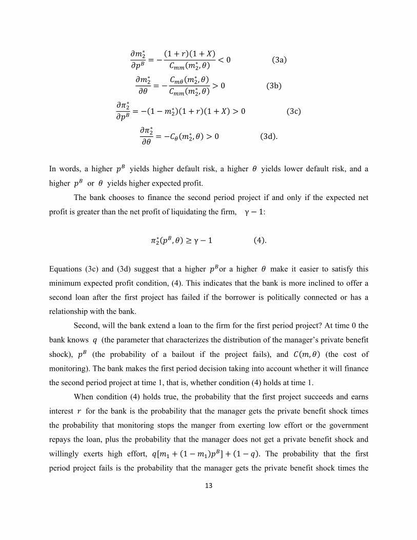
∗∗ , 0 3d .
In words, a higher yields higher default risk, a higher yields lower default risk, and a
higher or yields higher expected profit.
The bank chooses to finance the second period project if and only if the expected net
profit is greater than the net profit of liquidating the firm, γ 1:
∗ , γ 1 4 .
Equations (3c) and (3d) suggest that a higher or a higher make it easier to satisfy this
minimum expected profit condition, (4). This indicates that the bank is more inclined to offer a
second loan after the first project has failed if the borrower is politically connected or has a
relationship with the bank.
Second, will the bank extend a loan to the firm for the first period project? At time 0 the
bank knows (the parameter that characterizes the distribution of the manager’s private benefit
shock), (the probability of a bailout if the project fails), and , (the cost of
monitoring). The bank makes the first period decision taking into account whether it will finance
the second period project at time 1, that is, whether condition (4) holds at time 1.
When condition (4) holds true, the probability that the first project succeeds and earns
interest for the bank is the probability that the manager gets the private benefit shock times
the probability that monitoring stops the manger from exerting low effort or the government
repays the loan, plus the probability that the manager does not get a private benefit shock and
willingly exerts high effort, 1 1 . The probability that the first
period project fails is the probability that the manager gets the private benefit shock times the
14
probability that monitoring does not stop the manager from exerting low effort times the
probability that the government gives up bailout, with probability 1 1 .
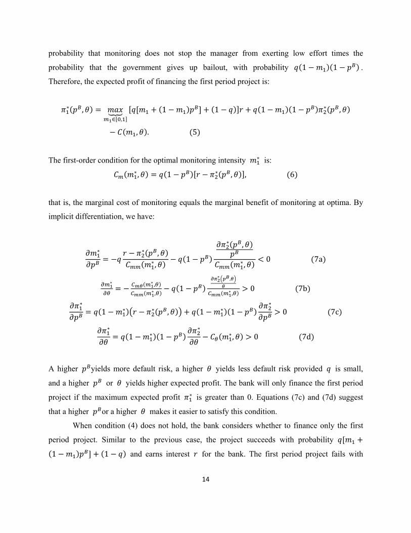
Therefore, the expected profit of financing the first period project is:
∗ ,∈ ,
1 1 1 1 ∗ ,
, . 5
The first-order condition for the optimal monitoring intensity ∗ is:
∗, 1 ∗ , , 6
that is, the marginal cost of monitoring equals the marginal benefit of monitoring at optima. By
implicit differentiation, we have:
∗ ∗ ,∗,
1
∗ ,
∗,0 7a
∗ ∗ ,∗ ,
1
∗ ,
∗ ,0 7b
∗
1 ∗ ∗ , 1 ∗ 1∗
0 7c
∗
1 ∗ 1∗
∗, 0 7d
A higher yields more default risk, a higher yields less default risk provided is small,
and a higher or yields higher expected profit. The bank will only finance the first period
project if the maximum expected profit ∗ is greater than 0. Equations (7c) and (7d) suggest
that a higher or a higher makes it easier to satisfy this condition.
When condition (4) does not hold, the bank considers whether to finance only the first
period project. Similar to the previous case, the project succeeds with probability
1 1 and earns interest for the bank. The first period project fails with
15
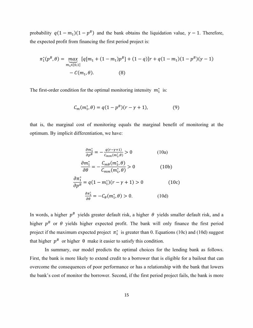
probability 1 1 and the bank obtains the liquidation value, 1. Therefore,
the expected profit from financing the first period project is:
∗ ,∈ ,
1 1 1 1 1
, . 8
The first-order condition for the optimal monitoring intensity ∗ is:
∗, 1 1 , 9
that is, the marginal cost of monitoring equals the marginal benefit of monitoring at the
optimum. By implicit differentiation, we have:
∗
∗ ,0 (10a)
∗ ∗,∗,
0 10b
∗
1 ∗ 1 0 10c
∗∗, 0. (10d)
In words, a higher yields greater default risk, a higher yields smaller default risk, and a
higher or yields higher expected profit. The bank will only finance the first period
project if the maximum expected project ∗ is greater than 0. Equations (10c) and (10d) suggest
that higher or higher θ make it easier to satisfy this condition.
In summary, our model predicts the optimal choices for the lending bank as follows.
First, the bank is more likely to extend credit to a borrower that is eligible for a bailout that can
overcome the consequences of poor performance or has a relationship with the bank that lowers
the bank’s cost of monitor the borrower. Second, if the first period project fails, the bank is more

16
likely to extend subsequent credit to a borrower eligible for government bail-out or having an
enduring relationship with the bank.15
4.2 Testable hypotheses and their relationship to the model
In our model, pB reflects the possibility that the government can intervene to rescue a
firm if it defaults on a loan, θ encapsulates the idea that monitoring and the banker-borrower
relationship can ease the lending process, and q reflects potential benefits to the manager of the
borrowing firm if a low level of managerial effort is elected. These forces affect the success of
the project and the bank’s decisions regarding initial and subsequent financing. We develop
testable hypotheses that relate to, and extend, these concepts. We also relate the testable
hypotheses to specific facets of China’s process of reform and development of the economy and
the banking system in particular.
We begin with predictions about the likelihood of getting bank loans and the likelihood
of default:
H1a: The likelihood of obtaining a bank loan increases if the borrower is politically
connected.
H1b: The likelihood of default increases if the borrower is politically connected.
In the model, a higher probability of a bailout reduces both the expected cost of borrower
default to the bank and the incentive of the bank to monitor. With less monitoring, the
borrower, in turn, is more likely to exert low effort and more likely to default. As a
consequence, a politically connected borrower is more likely to both obtain loans and
default on those loans.
H1c: The likelihood of obtaining a loan increases with the extent of the
relationship between borrower and bank. 15 These optimal choices for the lender and borrower match the empirical findings of Faccio, Masulis, and
McConnell (2006).

17
H1d: The likelihood of default decreases with the extent of the relationship
between borrower and bank.
In the discussion of the model, we note that a relationship between bank and borrower
should reduce the cost, θ, of monitoring the borrower. A lower cost of monitoring enables
a higher level of optimal monitoring and makes it more likely that the manager will exert
high effort and the project will succeed rather than failing and rendering the firm unable
to repay the loan. As a consequence, a borrower with a relationship with a lender is more
likely to obtain loans and less likely to default on those loans.
The model has clear implications for the likelihood that second-period financing
is obtained in the event of default on first-period financing:
H2: Following a default, the likelihood of subsequently obtaining credit increases
if the borrower is politically connected and increases with the extent of the
borrower - bank relationship.
H2 follows directly from the comparative statics of conditions (2) and (4) with respect to
the probability of a bailout, PB, and the cost of monitoring, θ, with our added assumption
that the cost of monitoring declines with the significance of the relationship between
bank and borrower.
Next, we offer predictions about the process of default resolution that go beyond
the model:
H3a: Following a default, resolution time decreases if the borrower is politically
connected, the borrower - bank relationship is extensive, or the lender is
politically influenced given the speed with which informal resolution can be
conducted.

18
H3b: Following a default, resolution time increases if the borrower is politically
connected, the borrower - bank relationship is extensive, or the lender is
politically influenced because informal resolution mechanisms are less efficient,
standardized, and predictable.
The idea behind H3a and H3b mirrors what we described above in our review of the
bankruptcy literature, that private organization can be less costly than a formal legal
process unless the debt structure is complicated (Gilson, John, and Lang, 1990; Asquith,
Gertner, and Scharfstein, 1994; Brunner and Krahnen, 2008). Under H3a, the
government or bank with a relationship with a borrower has an interest in the survival of
a borrower and expedites the process of default resolution. The government can enforce
its will with moral suasion or arm twisting. The lending bank can have easier access to
information and resources to speed the process of restructuring a loan to a borrower with
which there is a significant borrower-bank relationship. However, as in H3b, informal
mechanisms can be inefficient if the defaulting firm is large and complicated.
We also predict how the extent of economic development and reform or the
participation of a politically connected lender can affect the probability of default and the
likelihood of receiving subsequent financing afterwards:
H4: Borrowers from more developed regions receive fewer new loans or loans
subsequent to default because lenders are less prone to propping, and these
borrowers have lower odds of default due to more efficient monitoring.
Furthermore, a borrower’s political connections or relationship with a lender are
less valuable in such regions.
As the process of economic reform and development advances, government intervention is
reduced, competition among firms becomes more intense, the regulatory and legal system
becomes more efficient, and the gathering and processing of information is less costly.
Therefore, the need for a bailout is lower while the effectiveness of monitoring in discouraging
default is higher. Note that H4 offers no prediction about resolution time: higher quality
19
institutions can contribute to the quality of the default resolution process or they can be less
efficient than informal negotiation. We predict contrasting effects for borrowing from a Big
Five bank:
H5: Borrowing from a Big Five bank increases the likelihood of receiving new
loans, defaulting, and receiving subsequent financing, and decreases the default
resolution time, particularly for borrowers that are politically connected or have
an extensive relationship with a Big Five bank.
Big Five banks are more likely to function on non-commercial principles that advance political
goals. This reduces the efficiency of the banking system.
5. Database description and econometric specifications
5.1 The sample of bank loans
Our data on banks loans is provided by China’s bank supervising body, the China
Banking Regulatory Commission (CBRC). The CBRC database covers all commercial loans to
borrowers that hold at least one credit line of RMB 50 million or greater from at least one of the
largest 19 Chinese banks for the period from January 2007 to June 2013.16 The assets of these
banks account for over 80% of the market share of all commercial loans. They lend to
borrowers in 20 broad industrial sectors and 95 specific industries. After excluding loans from
the two development banks, excluding loans to financial services firms, and aggregating loans
between the same borrower and lender originating in the same month, our sample consists of
1,886,795 borrower-bank-months of new lending activity.17 From this data, we derive four
16 Our sample includes the Big Five very large state-owned commercial banks (Agricultural Bank of China, Industrial and Commercial Bank of China, Bank of China, People's Construction Bank of China, Bank of Com-munications) and twelve joint equity banks (China Citic Bank, China Everbright Bank, Huaxia Bank, China Guangfa Bank, Ping An Bank, China Merchants Bank, Shanghai Pudong Development Bank, Industrial Bank, China Minsheng Banking Corporation, Evergrowing Bank, China Zheshang Bank, and Bohai Bank). The CRBC database also includes loans from the two fully government owned development banks, China Development Bank and Export-Import Bank, but we exclude these loans because they are advanced explicitly for non-commercial policy-related purposes. 17 The raw database contains 7,179,136 loans and we end up with 1,886,795 borrower-bank-months. Less than two percent of the decline results from excluding loans from the two development banks and loans to financial
20
outcome variables that are the focus of our study. New Loans equals the amount of new
financing by borrower-bank-month. Default Occurrence is a dummy variable equal to one if
any of the outstanding loans between a particular borrower-bank pair are in default (that is, at
least three months overdue) during the month. Resolution Time is the longest number of months,
across all loans that are due in a particular borrower-bank-month, between the time a loan
defaults and the time the default is resolved. Subsequent Loan Availability after Default is a
dummy variable equal to one if a firm obtains a new loan from the same bank within three
months after defaulting on a loan from that bank that is due that month.
5.2 Borrower characteristics
Table A1 in the Appendix describes our proxies for political connections and
bank-borrower relationships, other loan and borrower characteristics obtained from the WIND
and CSMAR databases, and the four outcome variables just described above.18 We construct
proxy variables to indicate if a firm is politically connected as follows. The strategic industry
dummy equals one if the firm is in an industry that is considered strategically important by the
central government and zero otherwise. These industries (including mining, real estate, media
and culture, power, gas, and water, transportation and storage, banking, finance and insurance,
metals and non-metals, petrochemicals, and rubber) are typically supported, protected, and
monitored extensively by the central government.19 For firms listed on the Shanghai or
Shenzhen stock exchange, we also compute the SOE dummy equal to one if the firm is owned by
a government entity as indicated by the WIND database. Paralleling our proxies for political
connections, we create a measure of the extent of the relationship between a particular
institutions. Thus, aggregating loans between the same borrower-bank pair and occurring in the same month (Khwaja and Mian, 2008) explains the decline in observations from individual loans to borrower-bank-months. 18 Our loan dataset does not include loan interest rates but we used CSMAR for rates on bank loans to our sample of listed companies from the 17 commercial banks during our sample period. The average loan rate, 7.19%, is almost triple their standard deviation, 2.39%. 19 See discussion above, and www.chinadaily.com.cn/china/2006-12/19/content_762056.htm for an early official mention of strategic industries.
21
borrower-bank pair. Frequency equals the number of loans for each borrower-bank pair from the
start of our data to the current month.20
Other characteristics include firm size as measured with the book value of assets, firm
leverage, recent non-performing loan ratio of the firm, the number of lenders from which the
firm has obtained loans, 21 the size (measured as the book value of group assets) and
non-performing loan ratio of the group of firms which includes this borrower,22 and a dummy
variable to indicate a non-zero “risk signal” on at least one of five dimensions that bank
managers assess borrowers on, a dummy variable to indicate if a particular loan is granted by one
of the five big banks.23 Because development is uneven across China’s provinces (Jiang, Lee,
and Yue, 2010), we include the widely-cited regional development index of Fan, Wang, and
Zhang (2001). The index characterizes five aspects of economic development and financial
market reform for each province: the relationship between market and government, the
development of the non-state-owned economy, the development of product markets, the
development of markets for factors of production, and the development of market intermediaries
and the legal environment. Existing studies find that firms located in provinces with a higher
index value feature less government intervention, easier access to financial intermediaries, and
better intellectual property protection (Chen, Firth, and Xu, 2009). We also collect the annual
GDP growth rate of each province.
20 Frequency reflects the evolution of the depth of the relationship between a particular borrower-bank pair. Early research (Petersen and Rajan, 1994; Berger and Udell, 1995) uses the duration of the relationship but this measure is strongly correlated with borrower age and does not gauge the intensity of the relationship. 21 See Detragiache, Garella, and Guiso (2000) for theory and tests that highlight the significance of the number of banking relationships per borrower. In particular, Rodano, Serrano-Velarde, and Tarantino (2016) note how this variable can proxy for the difficulty of creditor negotiation and coordination regarding a distressed borrower. 22 CBRC indicates the primary group affiliation of each borrower in the loan database. Business groups can facilitate greater use of internal factor markets (Stein, 1997) and risk reduction through diversification and coinsurance (Khanna and Yafeh, 2007). Given limited contract enforcement, weak rule of law, corruption, and an inefficient judicial system, intragroup relationships are common and can be efficient (La Porta, Lopez-de-Silanes, and Shleifer, 1999; Chang, Khanna, and Palepu, 1999; Claessens, Djankov, and Lang, 2000). At the same time, deviations of voting rights from cash flow rights can enable controlling shareholders to gain effective control of a firm. As described or documented by Stulz (1988), Shleifer and Vishny (1997), Claessens, Djankov, Fan, and Lang (2002), and La Porta, Lopez-de-Silanes, Sheifer, and Vishny (2002), the resulting managerial entrenchment can affect corporate policies and firm value, and exacerbate agency problems (La Porta, Lopez-de-Silanes, and Shleifer, 1999; Claessens, Djankov, and Lang, 2000). 23 Qian, Strahan, and Yang (2015) find that lender risk assessments are better able to predict default after banking reforms in 2002 and 2003.
22
5.3 Econometric specifications
Our empirical approach centers on a set of regressions for each of the four outcome
variables. OLS regression models are used to explain New Loans and Resolution Time, while
binomial logistic regression models are used to explain Default Occurrence and Subsequent Loan
Availability after Default.
The OLS regression specification for New Loans and Resolution Time is:
Yi,j,t = β1X i,j,t + β2’Z i,j,t + ε i,j,t (11)
Yi,j,t is either the natural log of New Loans for the borrower i from bank j in month t or
Resolution Time equal to the longest number of months, across all loans of borrower i from bank
j that are due in month t, between the time a loan is default and the time the default is resolved.
Xi,j,t contains proxies for the borrower’s political connections and relationship with the lending
bank. In the sample of all borrowers, the Strategic Industry dummy measures the borrower’s
political connections. For the sample of listed borrowers, both the Strategic Industry dummy and
the SOE dummy measure political connections. In both samples, the Frequency variable
measures the relationship between the borrower and the lending bank. Zi,j,t contains firm and
group characteristics, market and macroeconomic conditions, year and industry fixed effects, and
a constant. β1 and β2 are slope coefficients and ε is the error term. Robust standard errors are
clustered at the firm level to account for heteroscedasticity across firms and serial correlations.
To explain Default Occurrence and Subsequent Loan Availability after Default, we use a
binomial logistic regression model:
P{Yi,j,t = 1} = F{β1’X i,j,t, β2’Zi,j,t, , ε i,j,t} (12)
In the Default Occurrence regression model, Yi,j,t is the Default Occurrence dummy equal to one
if any of the loans of borrower i from bank j in month t are in default. P{ Yi,j,t = 1} is the
probability that a default occurs. In the Subsequent Loans regression model, Yi,j,t is a dummy
variable equal to one if borrower i obtains a new loan from bank j within three months after
23
defaulting on a loan from bank j that is due in month t. P{ Yi,j,t = 1} is the probability that a
subsequent loan is obtained. F{·} is the logistic distribution function. As described previously,
Xi,j,t contains proxies for the borrower’s political connections and relationship with the lending
bank while Zi,j,t contains control variables, β1 and β2 are slope coefficients, ε is the error term,
and robust standard errors are clustered at the firm level.
We also estimate versions of specifications (11) and (12) that include interactive terms to
capture combinations of political connections, firm-bank relationships, and institutional factors
such as the Regional Development index and the lending bank’s status as one of the Big Five
state-owned banks. Another set of related regressions implements an identification strategy based
on difference-in-difference regressions and three exogenous events. At points in the presentation
of empirical results, we also include simple descriptive statistics on banks, lending, default, and
default resolution. Finally, we present some robustness tests of the significance of political
connections and the impact of stock market listing on the workings of default and its resolution.
6. Empirical results
6.1 Overview of banks, lending, and corporate default
Table 1 compares key characteristics of the Big Five banks and the twelve other
commercial banks in our sample. The scale of the Big Five is immediately evident as they
average over ten times as many employees and almost 20 times as many branches as other banks.
Annual book return on assets is, on average, about 20 basis points higher for Big Five banks, and
their fraction of income from non-interest sources, 19.893%, is three percent more than the
16.743% earned by other banks. Capital adequacy as a fraction of risk-weighted assets is
higher by 100 basis points or more for Big Five banks versus other banks, provisioning against
losses is higher, and Big Five banks enjoy higher economies of scale as measured by the ratio of
cost to income. However, the Big Five banks are substantially less liquid than the other sample
banks that enjoy a ratio of liquid assets to short-term liabilities, 27.914%, that is, on average, ten
percent higher. Furthermore, the fraction of non-performing loans for Big Five banks, 2.252%, is
more than double that of other banks.
Figure 3 plots indicators of economic development, the presence of politically influenced
firms, and the intensity of banking relationships across China’s provinces. Substantial variation
24
in characteristics across the provinces is evident. Panel A depicts differences in regional
development (an index of economic conditions and institutional quality) across provinces. As
can be seen, the coastal provinces close to Shanghai and Guangdong are the most developed
while the western provinces such as Xizang (Tibet) and Qinghai are least developed. Panel B
plots the proportion of total industrial assets owned by state owned enterprises (SOE) averaged
from 2007 to 2013. SOEs are predominant in the less developed western, central, and southwest
regions. Similarly, Panel C plots the proportion of industrial firms in strategic industries
averaged from 2007 to 2013. Strategic industries are more common in northern and southwestern
provinces. Panel D plots how dependent a borrower is on a particular lender averaged across
borrower-lender pairs from 2007 to 2013. Panel E plots how frequently a borrower borrows
from a particular lender averaged across borrower-lender pairs from 2007 to 2013.
Table 2 reports descriptive statistics for our outcome variables and borrower
characteristics across borrower-bank-months grouped by political connections and whether they
are listed on the stock market. A summary of the table’s key findings is as follows. The presence
of politically connected firms in the sample of borrowers is extensive. Close to 30% of
borrower-bank-months represent Strategic Industry borrowers. Over half of
borrower-bank-months for Listed Borrower are SOEs, and about 70% of listed Strategic Industry
borrower-bank-months represent SOE borrowers. Politically connected borrowers get larger
amounts of New Loans but they are larger firms (Assets), and the resulting amount of leverage is
only slightly higher for Strategic Industry or SOE borrowers relative to other borrowers. Among
All Borrowers, for example, the median New Loan amount is RMB 40 million for Strategic
Industry borrower-bank-months versus RMB 20 million for others. Median Assets is RMB 1.289
billion for Strategic Industry borrower-bank-months versus RMB 0.599 billion for others.
Politically connected borrowers have higher odds of Default Occurrence, odds of Subsequent
Loans, Risk Signal, and Group Assets. They have lower ROA and tend to be located in less
developed provinces. Listed borrower-bank-months, for example, have average odds of Default
Occurrence of 0.019 for SOE borrower-bank-months but only 0.012 for others. Across All
Borrowers, Strategic Industry borrower-bank-months have average odds of Subsequent Loans of
0.525 while others have odds of 0.475. Listed borrower-bank-months have larger New Loans,
Assets, number of Lenders, and Group Assets relative to All Borrowers. For example, median
25
Assets is RMB 0.713 billion for All Borrowers and RMB 3.654 billion for Listed Borrowers.
Listed borrowers borrow more frequently but are less dependent on a particular lender, which is
consistent with more information, alternative sources of financing, and confidence instilled by
being granted permission to list. Politically connected firms borrow more frequently and have a
lower dependence on a particular lender, which is consistent with government support which is
outlined in our model.24
Table 3 summarizes default occurrence across different types of borrowers. The first
group of rows partitions borrowers into those from strategic industries and others. Default
occurrence for strategic industry borrowers, 2.1%, is statistically significantly greater than the
rate, 1.7%, for non-strategic industry borrowers. However, this difference is not observed when
examining borrowers in provinces with below median regional development. Borrowers are
more likely to default on loans from Big Five lenders. The rate of default occurrence for
non-strategic firms borrowing from non Big Five banks, 0.8%, is particularly low. The next set
of rows compares default occurrence for high versus low Frequency borrowers. Low frequency
borrowers are statistically significantly more likely to default than other borrowers. Similarly, the
odds of default are greater for borrower-bank-months that score relatively low on Dependency.
Patterns for strategic versus non-strategic listed borrowers are similar to that for all borrowers,
though the general level of default occurrence is lower for listed firms. Default occurrence is
higher for politically-connected borrowers, particularly SOEs from below median developed
provinces or that borrow from a Big Five lender.
6.2 Explaining lending activity, default, and its aftermath
In this section, we use regression analysis to understand the behavior of our four outcome
variables, New Loans, Default Occurrence, Resolution Time, and Subsequent Loan Availability.
Each regression table includes a second panel that summarizes results using interactive terms
that relate Regional Development and Big Five Lender to other characteristics. Observations are
borrower-bank-months. Slope coefficients for the Strategic Industry and SOE dummies measure
whether political connections are correlated with the outcome variable. Slope coefficients on
24 Table A2 in the Appendix provides more detailed summary statistics broken down by the four outcome variables and by all borrowers versus listed borrowers.
26
Frequency and Dependence test whether the intensity of the borrower-bank relationship is
correlated with the outcome variable.
Table 4 presents OLS regressions to explain the natural log of New Loans, the amount of
new lending. Our model predicts political connections (H1a) or a relationship with a lender
(H1c) increase the likelihood that a borrower receives loans. Panel A presents basic
specifications. The Strategic Industry dummy variable has a positive and strongly statistically
significant slope coefficient across the four specifications that include it. Given that New
Loans is used in natural log form and is scaled by the natural log of assets among the explanatory
variables, slope coefficients have a straightforward interpretation. In Model 1 for All
Borrowers, for example, the slope of 0.179 indicates that the geometric mean of new loans as a
fraction of assets is 19.6% (e0.179 - 1) higher for a borrower from a strategic industry than for
other borrowers. The coefficient is of similar scale for both All Borrowers and Listed Borrowers,
though less statistically significant for the latter group. In contrast, the SOE dummy variable,
which is available only for Listed Borrowers, appears to be subsumed by the Strategic Industry
dummy.
Among the two variables that define the relationship between a particular borrower and
lender, the slopes on Frequency are strongly significantly negative, perhaps because some firms
receive a large number of relatively small loans. The slope coefficients on Dependency are
strongly significantly positive in all specifications that include this variable. For example, the
slope on Dependency in Model 3 for All Borrowers indicates that a one percentage point
increase in Dependency (loans from this particular bank as a fraction of all loans from all banks)
is associated with a 0.418% more New Loans for this borrower-bank-month.
Among the other findings in Panel A, the slope coefficients on the Big Five Lender
dummy suggest that these lenders offer larger amounts of loans in most cases (H5). Strongly
positive slopes that are less than one for the log of Assets suggest that, absent other conditions,
larger firms get smaller loans. The significantly positive slope coefficient estimates for
Nonperforming Loans in all specifications are particularly interesting. Troubled borrowers
appear to get more loans, not less, which suggests propping or bailouts. For example, the slope
coefficient of 0.108 in Model 1 for All Borrowers indicates that a one percentage point increase
in the percentage of Nonperforming Loans on a borrower’s balance sheet is associated with

27
0.11% more New Loans as a fraction of the borrower’s assets. In contrast, slope coefficients on
Group NPL are negative for All Borrowers and insignificant for Listed Borrowers. Strongly
negative slopes on the Regional Development index and GDP Growth of the borrower’s home
province suggest that lending is more extensive in less developed, slow-growing regions of the
country. Finally, the regression r-squared coefficients are large, specifically, 30% or more across
the specifications in Panel A.
Panel B summarizes specifications that seek to detect interactions among the explanatory
variables. There are a number of statistically significant interactions. For All Borrowers, a high
level of Regional Development dampens the positive association of New Loans with Strategic
Industry or Dependency (H4). The positive correlation of Strategic Industry dummy with New
Loans is larger when a loan is obtained from a Big Five Lender. While more frequent
borrowing is associated with reduced monthly new loan amount on average, this effect is
weakened if the loans are from a Big Five Lender, for both All Borrowers and Listed Borrowers.
On balance, the results for New Loans in Table 4 show strong evidence of political
effects at work. Firms from strategic industries and firms that borrow from Big Five banks get
more loans as a fraction of assets. Borrowers that are troubled, as indicated by nonperforming
loans, are supported with additional new loans. There is also evidence of relationship banking in
that dependence on a particular lender for a large fraction of outstanding loans is associated with
receiving more new loans. These political and relationship effects are particularly pronounced if
the borrower is located in a region which is relatively underdeveloped or slow-growing or if the
lender is a Big Five bank.
Table 5 presents logit regressions to explain the Default Occurrence dummy variable.
Our model predicts that political connections increase the likelihood that a borrower defaults
(H1b) while a relationship with a lender decrease the likelihood that a borrower defaults (H1d).
In Panel A, strongly significant positive slope coefficients on the Strategic Industry dummy are
consistent with H1b which predicts that the likelihood of default increases with the borrower’s
political connections. For example, the estimated slope of 0.113 in Model 1 for All Borrowers
implies that the odds of default are almost 12% greater for borrowers from a strategic industry.
The slope coefficients on the relationship variables, Frequency and Dependency, test H1d which
predicts that a more intense bank-borrower relationship reduces the likelihood of default. This
28
prediction is strongly confirmed with statistically significantly negative slopes on relationship
variables in almost all cases across all specifications. For example, the estimated slope of -0.118
on Dependency in Model 3 for All Borrowers indicates that a one percentage point increase in
Dependency is associated with a 0.12% decrease in the odds of default.
Among the other findings, the uniformly significantly positive slopes on the Big Five
Lender dummy are consistent with an increased risk of default when the lender is politically
connected (H5). For example, the estimated slope coefficient of 0.696 in Model 1 for All
Borrowers indicates that a loan from a Big Five lender has double the odds of default relative to
other loans. Uniformly significant negative slopes on the Regional Development index indicate
that the odds of default are greater for borrowers headquartered in relatively underdeveloped
provinces (H4). This is also the case for the regional GDP growth indicator for All Borrowers
specifications. Strongly positive slopes on Nonperforming Loans and Risk Signal, and strongly
negative slopes on ROA for Listed Borrowers, confirm that weak borrowers are more likely to
default.
Panel B measures the significance of interactive terms that combine political connections
or borrower-bank relationship with the Regional Development index or the Big Five Lender
dummy variable. Significant or marginally significant negative slopes on interactions of personal
political connections and regional development indicate that the increased likelihood of default
associated with borrower political connections is tempered in more developed regions (H4).
Interestingly, some significantly positive slopes on interactions of relationship proxies and
Regional Development indicate that the default-reducing value (H1d) of borrower-bank
relationships weakens in more developed regions. While this contradicts H4, it can indicate
less value from the borrower-bank relationship given less information asymmetry in more
developed regions. Significant or marginally significant positive slopes on interactive terms of
borrower political connections and Big Five Lender dummy indicate that default is particularly
likely for politically-connected firms borrowing from one of the politically-influenced Big Five
banks (H5). Finally, significantly positive slopes on interactive terms of relationship proxies and
Big Five Lender dummy indicate that the default-reducing value of a borrower-bank relationship
is weakened if the lender is a Big Five bank (H5).
29
In summary, the findings of Table 5 concerning Default Occurrence largely support our
basic themes. The political connections of borrowers are associated with a greater propensity to
default, and this is magnified by borrowing from a politically-influenced Big Five bank or
location in a relatively underdeveloped province. The extent of the borrower-bank relationship
contributes to reducing the likelihood of default, though this weakens if the lender is a Big Five
bank or the borrower is located in a highly developed province. Thus, the political connections of
borrowers and lenders seem to detract from the health of China’s banking system while
relationships between borrowers and lenders can enhance the system.
Table 6 presents OLS regressions to explain the natural log of default Resolution Time by
borrower-bank-month. We offer predictions, (H3a) and (H3b), about the impact of political
connections or a relationship with a lender for the resolution time of default. In Panel A, across
the political connections variables, there is only statistically marginal evidence that default
resolution time is reduced slightly for listed SOE firms (H3a). As an example, In Model 2 for
Listed Borrowers, resolution time is typically 17.2% shorter for SOE borrowers. Among the
borrower-bank relationship proxies, slope coefficients of about -0.1 on the natural log of
Frequency for All Borrowers imply that a 1% increase in Frequency is associated with about a
0.1% decrease in resolution time. There is stronger evidence that borrowing from a Big Five
lender results in a statistically significantly greater resolution time, which is consistent with H3b.
Furthermore, if nonperforming loans increase by one percentage point, resolution time increases
by about 0.25%, though not for listed firms. The effect is even larger for increases in the
borrower’s group NPL and is also found for the borrower’s Risk Signal. A higher level of
Regional Development is associated with longer resolution time, perhaps because more time is
required to satisfy more organized and formal procedures for resolving default or sort out
complex borrowers common from these better-developed regions. Finally, it is more time
consuming to resolve default for less profitable firms. For example, a one percentage point
increase in ROA is associated with a decrease in resolution time of more than 2% for listed
borrowers.
Panel B presents results of regressions that include interactive terms. There is only one
statistically significant interactive coefficient in the panel, and it indicates that resolution time
increases further if the defaulting borrower is located in a highly developed region and borrows
30
frequently from a particular bank. This suggests more complex borrowers, more time-consuming
formal default resolution procedures, or less benefit to privileged information in the more
developed regions.
Table 7 presents logit regressions to explain the Subsequent Loan Availability dummy
variable. In Panel A, there is much evidence that the odds of obtaining a new loan after default
are heightened if the borrower has political connections or a relationship with a particular lender
(H2). In Model 4 for All Borrowers, for example, the odds of obtaining subsequent financing are
almost 12% higher (e0.111 – 1) for borrowers from a strategic industry, increase by about 0.534%
for a 1% increase in Frequency, and increase by 0.957% for a one percentage point increase in
Dependency. The odds of receiving loans after default rise considerably if the lender is a Big
Five bank (H5) or, ironically, if the borrower has a relatively high level of nonperforming loans.
Most of these effects are more prominent for All Borrowers than for Listed Borrowers in
particular. Finally, based on ROA, relatively profitable firms have higher odds of subsequent
loans after default.
Paralleling the case for Resolution Time in Table 6, there are only a few significant
coefficients among the interactive variables in Panel B of Table 7. For All Borrowers, the odds
of receiving subsequent financing are lowered if the borrower is from a strategic industry and
located in a more developed region (H4), if there are frequent loans between the borrower and
bank and the borrower is located in a more developed region (H4), or if the borrower is highly
dependent on a Big Five lender (inconsistent with H5). The odds are greater if the borrower is
from a strategic industry and is seeking subsequent financing with a Big Five lender (H5). For
Listed Borrowers, the odds are lower if dependency is high and the borrower is located in a
relatively developed area (H4). Collectively, these findings suggest that regional development
plays a positive role in reducing propping from either government connections or a relationship
with the lender, while the combination of politically-connected borrower and lender exacerbates
propping.
6.3. Difference-in-difference analysis to further identification
Thus far, we have presented descriptive statistics and regression estimates that
characterize our novel and comprehensive data on bank loan defaults by Chinese corporations.
31
The facts we have presented are interesting and in many cases can be interpreted as supporting
the testable predictions we have advanced. In particular, we find that the political connections of
borrowers and lenders, borrower-bank relationships, and degree of development and economic
growth in the borrower’s province have significant associations with the process of lending and
default. Our next step is to design additional tests to more thoroughly identify the forces we
believe to be at work in the process of lending, default, and its aftermath among Chinese
corporate bank borrowers.
An increasingly common approach in the empirical corporate finance literature involves
difference-in-difference regressions centered on an exogenous event that has implications for the
predictions of our testable hypotheses, and, in particular, a differential predicted impact on
politically-connected or relationship borrowers versus other borrowers. We identify three such
events during our sample period.
First, China’s central government announced the new Enterprise Bankruptcy Law on 27th
August 2006 to be in effect on 1st June 2007. The law more clearly defines what happens if
default leads to bankruptcy, gives more power to creditors, and, in particular, reduces protection
for employee benefits. Given a relatively more well-defined process for resolving financial
distress, borrowers work harder to avoid default, creditors enjoy quicker resolution, and creditors
are less likely to prop up borrowers with more loans after default. The impact on resolution
time is ambiguous: as indicated by the US bankruptcy literature described above, informal
negotiations can sometimes be more efficient than taking a case to court.25 However, the
experience of politically-connected firms under the new law can differ if they continue to enjoy
special treatment.
Second, we predict that the Sichuan earthquake of 12th May 2008 affected the
creditworthiness and extent of government support of borrowers located in Sichuan province.
This event is a natural exogenous shock that we use to examine borrower vulnerability and
government bias towards politically-connected firms. Given the economic impact of the
earthquake, all corporate borrowers in Sichuan are more likely to default, and
25 Bankruptcy reform can also have broader benefits such as more lending, investment, and output. See Qian, Strahan, and Yang (2015), Ponticelli and Alencar (2016), Rodano, Serrano-Velarde, and Tarantino (2016), and Gormley, Gupta, and Jha (2016) for examples of institutional quality that differs across regions within one country, and Demirgüç-Kunt and Maksimovic (1998) for an overview of the benefits of a more efficient legal system.
32
politically-connected borrowers can be particularly vulnerable (H1b) given their inherent
weakness. However, politically-connected borrowers obtain more new loans relative to other
Sichuan firms (H1c) and firms in other provinces. Furthermore, politically-connected Sichuan
firms experience relatively quick resolution of default given government support (H3a) and
enjoy higher odds of getting subsequent loans (H2).
Third, China announced a massive RMB 4 trillion fiscal stimulus featuring increased
government spending on infrastructure, health, education, and tax decreases on 9th November
2008. We predict that, under the stimulus program, new credit is even more liberally allocated
to politically connected borrowers (H1a), thereby increasing the odds that they default (H1b).
Furthermore, politically connected borrowers enjoy additional privileges including faster
resolution of default (H3a) and greater odds of getting subsequent loans after default (H2) when
the economy is under pressure and, therefore, being supported by the government.26
Table 8 summarizes difference-in-difference regressions that detect responses to the
stimulus, earthquake, and new bankruptcy law events. The key coefficient in each of the three
sets of regressions is the slope on the interactive terms that isolates the treatment group and its
borrowing and default behavior in the period immediately after the event.
Panel A studies the entire sample of listed and private borrowers, with political
connection determined by whether or not a firm is from a strategic industry. The first set of
regressions centers on the new bankruptcy law of June 2007. The significantly positive slope on
Event x Strategic dummy for default occurrence and the marginally negative slope for default
resolution time indicate that, after the announcement of the new bankruptcy law, the odds of
default are higher (H1b) and default resolution time is lower (H3a) for politically-connected
firms. In contrast, the slopes on the event dummy term indicate that all borrowers experience
lower odds of default and lengthier default resolution under the new bankruptcy law which
suggests that informal negotiations can be more efficient than more formal procedures.
Therefore, these findings highlight the privileged experience of politically connected firms under
the new law: they continue to display poor performance while enjoying quick re-negotiation after
default.
26 If rollovers and informal activities (that occur before maturity) increase for privileged firms during an economic downturn, this will bias our findings downwards.

33
The second set of regressions centers on the Sichuan earthquake of May 2008. The key
variable is the triple difference-in-difference interactive, Event x Strategic dummy x Sichuan
headquarters dummy, because it isolates the precise group of firms and time period for which we
predict a different response to the event. Across the four regressions, the sole statistically
significant slope coefficient on default occurrence indicates relatively greater odds of default for
Sichuan-based strategic industry firms after the earthquake (H1b). Note that the number of listed
Sichuan-based firms is small,27 and this can weaken the significance of the estimates.
The third set of regressions centers on the fiscal stimulus announced in November 2008.28
The estimated slopes on the Event x Strategic dummy variable across the four regressions
indicate that, after the announcement of the fiscal stimulus, politically-connected firms display
worse behavior: their odds of defaulting increase (H1b). At the same time, they experience
relatively indulgent treatment: they borrow more (H1a), experience faster default resolution
(H3), and enjoy greater odds of receiving subsequent loans (H2). The slope coefficient on the
Event dummy in the default occurrence regression is particularly notable. It is strongly
significantly negative, indicating that borrowers typically default less after the stimulus event, in
contrast to the positive slope for politically-connected Sichuan firms.
Thus, across all the results in Panel A, politically connected firms are significantly
different from other borrowers. They perform relatively poorly yet enjoy advantages in
borrowing and resolving default. We also note that the parallel trends tests are almost entirely
insignificant, except for a marginally significant coefficient in the New Loans regression for the
earthquake event. This is consistent with the idea that the difference-in-difference findings are
not driven by trends in control versus treated borrower characteristics.
In Panel B, the sample is confined to listed firms only. We classify firms with political
connections in two ways, membership of a strategic industry or state ownership (SOE). The
27 The New Loans sample is the largest among our four outcome variables and has 1,886,795 total observations, 53,957 with Sichuan dummy equal to one, and 8102 observations with Sichuan x Strategic Event equal to one. New Loans for listed firms only has 86161 total observations, 2681 with Sichuan dummy equal to one, and 337 with Sichuan x Strategic x Event equal to one. Sample sizes are even smaller for the other three outcome variables as they include only borrower-bank-months associated with default.
28 There is overlap between the earthquake and fiscal stimulus event windows but the addition of the Sichuan headquarters dummy allows us to distinguish the earthquake effect.
34
first set of regressions centers on the new bankruptcy law of June 2007. The estimated slope
coefficients on the Event x Strategic Industry dummy variable suggest no significant differences
in lending, default, and resolution conditions for listed politically connected firms after the
announcement of the new bankruptcy law. There is marginal evidence from the Event x SOE
dummy that listed SOE borrowers get more new loans and have greater odds of getting
subsequent loans under the new bankruptcy law, which is consistent with continued indulgent
treatment in spite of the reforming spirit of the new law.
The second set of regressions centers on the Sichuan earthquake of May 2008. The key
variable is the triple difference-in-difference interactive, Event x SOE dummy x Sichuan
headquarters dummy. The estimated slope coefficients indicate that listed strategic industry firms
headquartered in Sichuan experience significantly less new loans, marginally longer resolution
time, and lower odds of receiving subsequent loans. Somewhat similar but weaker effects are
observed for SOE borrowers. Thus, politically connected listed borrowers experience less
indulgent conditions than other borrowers after the earthquake event, which contradicts H4.
The third set of regressions centers on the fiscal stimulus announced in November 2008. The
results for SOE borrowers are broadly similar to those for all politically connected borrowers in
Panel A.
6.4 Stock market listing and lending outcomes
Throughout the presentation of our findings on the four borrowing outcome variables, we
have noted differences between unlisted and public borrowers. Companies must be approved for
trading on an organized market. Furthermore, listing on a stock market imposes disclosure
requirements and the scrutiny of investors and regulators. In the context of our model, stock
market listing can shift down the cost of monitoring function, , and, thus, affect
borrowing outcomes. This effect should vary with the extent of the borrower-bank relationship,
θ, and potential political influences, .
In this section, we examine the impact of stock market listing with a matched estimator
comparison of the four outcome variables across listed and unlisted borrowers categorized by
political connections and borrower-bank relationships. Because listing is not exogenous, we
35
address selection effects as follows (Lemmon and Roberts, 2010).29 First, we create a dummy
variable for each borrower-month equal to one if the firm is trading on a Chinese stock exchange
in that month and zero otherwise. This becomes the dependent variable in a probit regression
with independent variables similar to the basic outcome regression specifications (Tables 4
through 7) but excluding the relationship (Frequency, Dependency) and political influence
(Strategic Industry, SOE) indicators.30 Second, we match each listed borrower-month with a
non-listed borrower from the same month. To check the fit of the matching, we examine the
slope and pseudo r-squared coefficients from a second probit regression using the listed
borrower-months and their matches. Third, we compute average differences of each outcome
variable, comparing listed borrowers to unlisted borrowers, and for subsets based on the political
influence and relationship indicators.
Additional details of our propensity score matching process are as follows. First, we
perform propensity score matching four times, once for each of the four outcome variable
samples. This is necessary given differences in sample sizes and problems that can arise after
loan is granted. For example, suppose a listed borrower-month is matched to an unlisted
borrower-month in the New Loans sample. This pair will not work for computing averages of
Default Occurrence if default was not resolved within our sample period for both borrowers. It
will not work for computing Resolution Time or Subsequent Loans unless both firms defaulted.
Thus, we conduct matching for each of the four outcome variables separately using the
respective regression sample.
Second, for each treated and control borrower-month observation in each of the four
matched samples, we return to the original regression sample and identify borrower-bank-month
observations for the same borrower and month. There is more than one borrower-bank-month
observation associated with each borrower-month if the firm borrowed from more than one
lender that month. For each outcome, we compute the average difference across listed and
29 Official documents indicate size, public float, record of positive earnings, and lack of accounting and legal problems affect the likelihood of approval for listing (http://english.sse.com.cn/laws/framework/c/3978488.pdf). However, there is no precise formula and listing decisions likely reflect political considerations as well (Aharony, Lee and, Wong, 2000). Thus, we cannot apply a Heckit procedure since we cannot apportion explanatory variables between the treatment probit and the outcome regressions. We cannot employ a regression discontinuity approach because we cannot observe the criteria or the threshold. Recent evidence (Allen, Qian, Shan, Zhu, 2017) suggests that unlisted Chinese firms perform better than those selected for A share listing. 30 We do not match on political influence or relationship proxies because we will measure differences across subsets of firms created from these measures.
36
unlisted borrowers and the average difference-in-difference across listed and unlisted borrowers
characterized by political connections or bank-borrower relationships. Third, we implement
propensity score matching with nearest neighbor set to one and a caliper of 0.01.31 To check the
robustness of our findings, the appendix presents a variety of other estimates based on different
values for nearest neighbor and caliper.
Table 9 presents the results on stock market listing and lending outcomes in two panels.
The effectiveness of our propensity score matching scheme for the New Loans sample is evident
in Panel A. The pseudo r-squared goes from 26.4% for the pre-match probit to 0.4% for the
post-match probit. This indicates that the matching process purges almost all of the differences in
characteristics of the treated borrower-months and their matched controls. While some of the
differences in covariate values between treated and matched observations remain statistically
significant, their economic significance is often low. For example, after matching, average
leverage is 0.535 for treated observations and 0.543 for control observations. The probits for the
Default Occurrence, Resolution Time, and Subsequent Loan samples show low pre-match
pseudo r-squared, even lower post-match pseudo r-squared, and fewer statistically significant
differences in covariates across treated and control observations. Thus, among borrowers that
have defaulted, there are few substantial differences between listed and unlisted firms for the
characteristics we can measure. However, conclusions about Resolution Time and Subsequent
Loans are limited by the small sample sizes that emerge from the matching process.
Panel B examines the associations between listing and the four outcome variables. Across
all borrowers, listed firms take on significantly less New Loans (on average, RMB 159,000 less)
and enjoy marginally significantly quicker Resolution Time (on average, 0.21 fewer months) if
they default. This is consistent with listed borrowers enjoying alternatives to bank financing
and quicker resolution when problems arise. Differences in Default Occurrence and Subsequent
Loans do not differ significantly across listed and unlisted borrowers. In contrast, strategic
industry borrowers take on significantly more New Loans (on average, RMB 11.43 million
more) and experience longer Resolution Time (on average, 6.024 months more) if they default.
31 The caliper is a maximum distance restriction on potential controls selected to match a treated observation. A smaller caliper excludes poorer matches at the potential cost of fewer observations. See Lins, Volpin, and Wagner (2013) for a discussion and application. Table A6 in the Appendix describes robustness tests based on differing values for the caliper and nearest neighbor parameters. Findings are invariant to changes in these parameters.
37
When compared to the averages for all borrowers, the net average effects for strategic industry
borrowers are RMB 11.589 million (11.430 + 0.159) more New Loans and 6.234 months
(6.024+0.210) months quicker Resolution Time after listing. The increased Resolution Time can
be a plus if it represents fewer rapid but opaque bailouts and under-the-table workouts.
Furthermore, there is marginally significant evidence that these borrowers default less frequently
and are less likely to receive Subsequent Loans if they are listed. Thus, there is evidence that
borrowing binges by politically connected firms continue after listing but other aspects of their
lending process improve.
Across the two relationship proxies, New Loans increases (on average, by RMB 4.797
million relative to all borrowers) for High Frequency borrowers but declines (on average, by
RMB 2.428 million relative to all borrowers) for High Dependency borrowers. Put another way,
borrowers with a diversity of banking relationships borrow even more once listed while
borrowers more dependent on particular bank obtain less New Loans from that particular lender
after listing. This suggests that borrowers are less dependent on a primary lender once listed on a
stock market, thereby reducing the hold-up problem. There is marginally significant evidence
that high relationship borrowers are relatively more likely to default after listing. This suggests
that the value of relationship banking in dealing with financial distress declines as it is replaced
by stock market listing. Finally, there is strongly significant evidence of quicker (on average, by
almost 5 months relative to all borrowers) resolution of default for High Frequency borrowers
that are listed, and marginally significant evidence of greater ease in obtaining Subsequent
Loans. On balance, the results presented in Table 9 suggest that stock market listing is associated
with improvements in some dimensions of lending outcomes.
6.5 Robustness tests
To check our findings, we present several robustness tests. They are intended to check the
delinquency period used to define default, the proxies for political influences, and the proxies,
Frequency and Dependency, for borrower-bank relationships.
6.5.1 The delinquency window and the default dummy
38
Table 10 assesses the sensitivity of our default outcome measures to the length of the
delinquency period that is used to define the default occurrence dummy. Default occurs if the
borrower is at least three, six, or twelve months overdue on at least one loan from this bank for
the current borrower-bank-month observation. Across All Borrowers, average Default
Occurrence declines from 1.8% to 0.6% as the definition of default is extended from three
months overdue to twelve months overdue, as is expected because most troubled loans do not
stay in default for many months. The increased default risk of Strategic Industry borrowers or
low relationship borrowers remains significantly greater than that of other borrowers regardless
of delinquency horizon. Across All Borrowers, Resolution Time rises from 7.73 to 10.15
months as the default horizon increases from three to twelve months. Difference in Resolution
Time for Strategic Industry or High Frequency versus other borrowers is not strongly affected by
the default horizon. The odds of receiving Subsequent Loans, and differences in those odds
across borrower types, change only slightly as the default horizon is increased from three months
to one year. Thus, it seems that changing the default window does not radically alter patterns in
outcome variables across types of borrowers.
6.5.2 Alternative definitions of borrower political connections
Table 11 examines alternative proxies for borrower political connections.32 Panel A
studies the All Borrowers sample while Panel B is listed borrowers only.
The extent of government control or influence over a particular Chinese firm can go far
beyond explicit government ownership (Milhaupt and Zheng, 2015). Therefore, we test several
additional proxies for political connections. Provincial Capital dummy equals one if the firm is
headquartered in a provincial capital. Provincial capitals, the economic and political center of a
province, can subject a borrower to greater political influences or can offer an institutional
environment that is better than other locations in the province. Development Bank dummy equals
one if the borrower has ever obtained a loan from China Development Bank or Export-Import
Bank of China during or prior to the current month. These institutions are intended to explicitly
32 Additional specifications split the state-owned dummy into central government versus local government controlled, but the results are almost entirely insignificant. See Huang, Li, Ma, and Xu (2017) for discussion of potential differences due to the level of government that controls an enterprise.

39
serve non-commercial development goals as directed by the government. Personal Political
Connection is a dummy variable equal to one if the borrower’s top management has strong ties to
the Communist party or the Peoples Liberation Army as of the beginning of the calendar year.
These firms can enjoy a different relationship with some lenders than other borrowers. Note that
the information needed to construct this variable is only available for listed firms. Turnover
Event is a dummy variable equal to one if borrower’s headquarters province has changed
governor or party secretary within the calendar year or previous calendar year (Piotroski and
Zhang, 2014). An impending change in political leadership can affect the process of
borrowing, default, and default resolution by changing expectations of the provincial
government’s goals and incentives, the effectiveness of local institutions, and the political
connections of particular firms.
A summary of Panel A’s findings for All Borrowers is as follows. For New Loans, slope
coefficients for Provincial Capital and Development Bank are significantly positive and of
similar scale. This is consistent with H1a and the results of the Table 4 regressions to explain
New Loans. The slope coefficient on Turnover Event is significantly negative as is the
coefficient for Turnover Event x Strategic Industry. This is consistent with outgoing or incoming
political leaders restraining careless lending, particularly to borrowers in strategic industries.33
This is not consistent with borrowers rushing to exploit their political connections and obtain
more loans prior to the change in leadership. For the odds of Default Occurrence, the slope on
Turnover Event x Strategic Industry is marginally significantly positive, which is consistent with
H1b and some of the results in Table 5. The slope coefficient on Provincial Capital is
significantly negative. Though this suggests political influence related to physical location in an
administrative center, the sign is opposite to the prediction of H1b. For Resolution Time, there is
only one significant result, a negative slope coefficient on Provincial Capital. This is consistent
with H3a, that is, expedited default resolution for politically connected borrowers, and parallels
what is reported in Table 6. For the odds of a Subsequent Loan, slopes are marginally
significantly positive on Strategic Industry and Development Bank, which is consistent with
33 A broadly related phenomenon is the finding of Piotroski and Zhang (2014) that Chinese IPO activity accelerates prior to a change in provincial political leadership, either to enhance the outgoing leadership’s perceived capital market development or monetize political connections before they vanish.

40
H1a, H5, and the results reported in Table 7. The slope coefficients on Turnover Event x
Strategic Industry in the New Loans and Subsequent Loans regressions suggest that political
leaders seek a smooth transition by restricting default-prone new loans but encouraging
subsequent loans to stave off further defaults or even bankruptcies.
A summary of Panel B’s findings for Listed Borrowers is as follows. The results for New
Loans to Listed Borrowers are similar to those for All Borrowers in Panel A and confirm H1a.
Slope coefficients for Provincial Capital and Personal Political Connection are marginally
significantly positive. The slope coefficient on Turnover Event x SOE is significantly negative,
and, as above, can represent political pressure on outgoing and incoming leaders to control risks
in the banking system. The results for the odds of Default Occurrence for Listed Borrowers echo
the findings for All Borrowers in Panel A. Slopes on Turnover Event x Strategic Industry and
Turnover Event x SOE are significantly or marginally significantly positive. The slope on
Provincial Capital is significantly negative. For Resolution Time, there are no significant slope
coefficients. For the odds of a Subsequent Loan, the slope is significantly positive on Personal
Political Connection, which is consistent with H1a. The slope coefficient on Provincial Capital is
marginally significantly negative, which echoes H4. The slope coefficients on Turnover Event
x Strategic Industry and Turnover Event x SOE are marginally significantly positive, echoing
what is reported for All Borrowers in Panel A.
6.5.3 Checking the robustness of the relationship proxies Frequency and Dependency
A novel dimension of our findings is the apparent significance of relationship banking to
China’s financial system. However, there is the obvious concern that our proxies, Frequency
and Dependency, are in some way endogenous or masking some underlying factor other than
relationship banking (Bharath, Dahiya, Saunders, and Srinivasan, 2011). To address this
concern, we parallel the procedure outlined previously to study the impact of stock market
listing. The dependent variable for these probit regressions equals one if the particular
borrower-bank-month scores high on borrower-bank relationship (that is, in the top quartile), else
equals zero if the observation scores low (that is, in the bottom quartile). The two middle
quartiles are excluded from these computations. The results of the propensity score matching
allow us to pair each high relationship borrower-bank-month with a low relationship
41
borrower-bank from the same month. As we did for the listing effect, we check the fit of the
matching with a second post-match probit regression using the high relationship
borrower-bank-months and their matches. We compute average differences of each outcome
variable, comparing high and low relationship borrower-bank-months. As before, we perform
propensity score matching four times, once for each of the four outcome variable samples.
Furthermore, we have two proxies for relationship, Frequency and Dependency, so we run the
entire procedure twice, that is, once for each of these two proxies. Finally, we implement
propensity score matching with nearest neighbor set to one and a caliper of 0.01.
The results of this test are reported in Table A5 in the Appendix. For Frequency (Panels
A and B), significance of the slope and adjusted pseudo r-squared coefficients is reduced sharply
when comparing pre-matching and post-matching probits for each of the four outcome variable
samples, indicating a successful matching process. The average mean differences in the outcome
variables between the treated borrower-bank-month observations and the matched control
observations suggest effects of bank-borrower relationships that are similar to those of the main
regression results in Tables 4 to 7. On average, the amount of new loans to high frequency
borrowers is RMB 0.466 million less than to low frequency borrowers. Compared to low
frequency borrowers, the likelihood of default occurrence by high frequency borrowers is 0.1
percentage point lower, the default resolution time is 1.304 months shorter, and the likelihood of
obtaining subsequent loans after default is 40.3 percentage points higher. For Dependency
(Panels C and D), there is much less of a decline in pre-matching versus post-matching pseudo
r-squared, thus indicating a less successful match. Compared to low dependency borrowers, high
dependency borrowers borrow RMB 1.010 million more in new loans, the likelihood of default
occurrence is 0.7 percentage point lower, the default resolution time is 0.09 months shorter, and
the likelihood of obtaining subsequent loans is 6.2 percentage points higher. These results,
particularly for Frequency, suggest that an enduring borrower-bank relationship is typically
associated with more positive loan outcomes and favorable default resolution.34
34 Additional robustness tests add bank × year fixed effects to control for unobservable bank characteristics (while omitting the Big Five dummy) or borrower × year fixed effects to control for unobservable borrower characteristics. They serve to further check the apparent strength of our bank-borrower relationship proxies. Results (presented in Tables A3 and A4) largely confirm those in Tables 4 through 7.
42
7. Summary and conclusions
Our raw database of over seven million loans represents virtually all significant loans
from the largest 17 Chinese commercial banks to corporate borrowers across China from January
2007 to June 2013. A number of dimensions of our empirical findings suggest that Chinese
banking sometimes contradicts classic notions of insider debt and the relative efficiency of
private renegotiation of default. We confirm some prior beliefs: borrowers from
government-designated strategic industries or owned by the state default more frequently and
typically perform poorly after default. Big Five state owned banks and poor regional
development aggravate these effects, while some dimensions of the default outcomes of
politically-connected borrowers worsen after bankruptcy law improvements or fiscal stimulus.
However, we find significant evidence of beneficial relationship banking, in spite of
potential “soft budget” and “hold-up” problems and the incomplete development of China’s
financial system. Furthermore, stock market listing seems to improve some facets of lending
outcomes depending on the type of borrower. Thus, the reform and development of China’s
financial system is proceeding on some dimensions but continuing old practices in others, and
the pace of these changes varies across different parts of the country.
Though the Chinese government has vowed to bring discipline to China’s borrowers and
lenders, China’s first corporate default on a domestic bond, by Chaori Solar in 2014, led to a
bailout of the firm’s creditors and continued partial operation by the borrower.35 Furthermore,
Sichuan Coal Industry Group, a large firm in a weak industry, overcame a seemingly
catastrophic bond default within several weeks with help from the provincial government and
banks.36 At an October 2016 meeting of Communist Party officials, President Xi Jinping stated:
“Party leadership and building the role of the party are the root and soul for state-owned
enterprises. The party’s leadership in state-owned enterprises is a major political principle, and
that principle must be insisted on.”37 On the other hand, in September 2016, an unlisted
company owned by a provincial government, Guangxi Nonferrous Metals, was unable to
overcome default and was declared bankrupt by a court. Therefore, the tension between political
goals and economic reform continue to affect the workings of the occurrence and resolution of
35 “Chinese Debt: A Moral Deficit“, The Economist, 18th October 2014. 36 See http://www.shanghaidaily.com/business/energy/Sichuan-coal-firm-pays-bond-fully/shdaily.shtml. 37 See http://www.nytimes.com/2016/10/14/world/asia/china-soe-state-owned-enterprises.html?_r=0.
43
corporate defaults in China. Other looming issues related to resolving credit problems involve
everything from non-bank financial products to municipal debt,38 in addition to many problems
among corporate borrowers. The Chinese case illustrates the contradictions that arise in a
financial system that is evolving away from central planning. Improvements in the process of
lending, default, and default resolution are evident, yet weak performance and state support for
politically connected borrowers persist.
38 See Gao, Ru, and Tang (2016) for evidence on the size of this looming problem.
44
References
Aharony, J., C. J. Lee and Wong, T. J., 2000, Financial packaging of IPO firms in China, Journal of
Accounting Research 38, 103 - 126.
Allen, F., J. Qian, and M. Qian, 2005, Law, Finance and Economic Growth in China, Journal of
Financial Economics 77, 57–116.
Allen, Franklin, Qian, Jun, Shan, Susan Chenyu, and Zhu, Lei, 2017, Dissecting the Long-Term
Performance of the Chinese Stock Market (6th January). Available at SSRN:
https://ssrn.com/abstract=2880021 or http://dx.doi.org/10.2139/ssrn.2880021
Ang, James, Cheng, Yingmei, and Wu, Chaopeng, 2014, Does Enforcement of Intellectual Property
Rights Matter? Evidence from Financing and Investment Choices in the High Tech Industry, The
Review of Economics and Statistics 96, 332 – 348.
Asquith, Paul, Robert Gertner, and David Scharfstein, 1994, Anatomy of financial distress: An
examination of junk-bond issuers, Quarterly Journal of Economics 109, 625 - 658.
Ayyagari, M., A. Demirguc-Kunt, V. Maksimovic, 2010, Formal versus Informal Finance: Evidence
from China, Review of Financial Studies, 23, 3048 - 3097.
Bailey, W , Huang, V., and Yang, Z., 2011, Bank loans with Chinese characteristics: Some evidence on
inside debt in a state controlled banking system, Journal of Financial and Quantitative Analysis
46, 1795 – 1830.
Berger, Allen N. and Gregory F. Udell, 1995, Relationship Lending and Lines of Credit in Small Firm
Finance, Journal of Business 68, 351 - 381.
Berger, A., and G. Udell, 2006, A more complete conceptual framework for SM finance, Journal of
Banking and Finance 30, 2945 – 2966.
Berglof, E. and L. Von Thadden, 1994, Short-Term versus Long-Term Interests: A Model of Capital
Structure with Multiple Investors, Quarterly Journal of Economics 109, 1055 – 1084.
Bertrand, M., P. Mehta, and S. Mullainathan, 2002, Ferreting out tunneling: An application to Indian
business groups, Quarterly Journal of Economics 117, 121 – 148.
Bharath, Sreedhar T., Dahiya, Sandeep, Saunders, Anthony, and Srinivasan, Anand, 2011, Lending
Relationships and Loan Contract Terms, Review of Financial Studies 24, 1141 - 1203.
Bodenhorn, Howard, 2003, Short-Term Loans and Long-Term Relationships: Relationship Lending in
Early America, Journal of Money, Credit and Banking 35, 485 - 505.
Bolton, Patrick, Freixas, Xavier, Gambacorta, Leonardo, and Mistrulli, Paolo Emilio, 2016, Relationship
and Transaction Lending in a Crisis, Review of Financial Studies 29, 2643 - 2676.
45
Boot, A., 2000, Relationship banking: What do we know? Journal of Financial Intermediation 9, 7 - 25.
Boot, A., and A. V. Thakor, 2000, Can relationship banking survive competition? Journal of Finance 55,
679 – 813.
Borisova, Ginka and William L. Megginson, 2011, Does Government Ownership Affect the Cost of
Debt? Evidence from Privatization, Review of Financial Studies, 24, 2693-2737.
Brunner, Antje and Jan Pieter Krahnen, 2008, Multiple Lenders and Corporate Distress: Evidence on
Debt Restructuring, The Review of Economics Studies, 75, 415 -m442.
Chang, C., G. Liao, X. Yu, and Z. Ni, 2014, Information from Relationship Lending: Evidence from
Loan Defaults in China, Journal of Money, Credit, and Banking 46, 1225 - 1257.
Chang, J., T. Khanna, and K. Palepu, 1999, Transparency in emerging markets: The extent and accuracy
of analyst activity, working paper, The Wharton School and Harvard Business School.
Chen G. M., M. Firth, and L. P. Xu, 2009, Does the Type of Ownership Control Matter? Evidence from
China’s Listed Companies, Journal of Banking and Finance, 33, 171-181.
Chen, Y. L , M. Liu, and J. Su, 2013, Greasing the wheels of bank lending: Evidence from private firms
in China, Journal of Banking and Finance, forthcoming.
Claessens, S., S. Djankov, and L. H. P. Lang, 2000, The separation of ownership and control in East
Asian corporations, Journal of Financial Economics 58, 81 - 112.
Claessens, S., S. Djankov, J. P. H. Fan, and L. H. P. Lang, 2002, Disentangling the incentive and
entrenchment effects of large shareholdings, Journal of Finance 57, 2741 – 2771.
Cull, Robert, and Xu, Lixin Colin, 2005, Institutions, ownership, and finance: the determinants of profit
reinvestment among Chinese firms, Journal of Financial Economics 77, 117 – 146.
Demirgüç-Kunt, Asli, and Maksimovic, Vojislav, 1998, Law, Finance, and Firm Growth, Journal of
Finance 53, 1540 – 6261.
Detragiache, E., Garella, P. and Guiso, L., 2000, Multiple versus Single Banking Relationships: Theory
and Evidence, Journal of Finance 55, 1133–1161.
Dewatripont, M., and E. Maskin, 1995, Credit and efficiency in centralized and decentralized
economies, Review of Economic Studies 62, 541 – 555.
Diamond, D., 1991, Monitoring and reputation: the choice between bank loans and privately placed
debt, Journal of Political Economy 99, 689 – 721.
Diamond, D. W., and P. H. Dybvig, 1983, Bank Runs, Deposit Insurance, and Liquidity, Journal of
Political Economy 91, 401 – 419.
46
Djankov, Simeon, Oliver Hart, Carlee McLiesh, and Andrei Shleifer, 2008, Debt Enforcement around
the World, Journal of Political Economy, 116, 1105 - 1149.
Dobson, W., and A. K. Kashyap, 2006, The Contradiction in China's Gradualist Reforms, Working
Paper, University of Chicago.
Duchin, Ran, and Sosyura, Denis, 2012, The Politics of Government Investment, Journal of Financial
Economics 106, 24 – 48.
Duchin, Ran, and Sosyura, Denis, 2014, Safer Ratios, Riskier Portfolios: Banks’ Response to
Government Aid, Journal of Financial Economics 113, 1 – 28.
Dybvig, P.H., S. C. Shan, and T. Tang, 2012, Outsourcing Bank Loan Screening: Evidence from Third
Party Credit Guarantees, working paper.
Everett, C. R., 2010, Group membership, relationship banking and loan default risk: the case of online
social lending, Working paper, Purdue University.
Facio, M., R. Masulis, and J. J. McConnell, 2006, Political connections and corporate bailouts, Journal
of Finance 61, 2597 – 2635.
Fama, E. F., 1985, What’s Different about Banks?, Journal of Monetary Economics 15, 29 –39.
Fan G, X. L. Wang and L. W. Zhang, 2001, NERI INDEX of Marketization of China’s Provinces 2001
Report, Journal of National School of Administration 3, 17 - 27 (in Chinese).
Fan, Joseph P.H., Huang, Jun, and Zhu, Ning, 2013, Institutions, ownership structures, and distress
resolution in China, Journal of Corporate Finance 23, 71 – 87.
Favara, Giovanni, Enrique Schroth, and Philip Valta, 2012, Strategic Default and Equity Risk Across
Countries, Journal of Finance, 67, 2051-2095.
Franks, Julian R., and Walter N. Torous, 1994, A comparison of financial re-contracting in distressed
exchanges and Chapter 11 reorganizations, Journal of Financial Economics 35, 349 - 370.
Gao, Haoyu, Ru, Hong, and Tang, Dragon Yongjun, 2016, Subnational Debt of China: The
Politics-Finance Nexus, unpublished University of Hong Kong working paper.
Gilson, Stuart C., 1997, Transactions costs and capital structure choice: Evidence from financially
distressed firms, Journal of Finance 52, 161 - 196.
Gilson, Stuart C., Kose John, and Larry HP Lang, 1990, Troubled debt restructurings: An empirical
study of private reorganization of firms in default, Journal of Financial Economics 27, 315 - 353.
Gopalan, R., V. Nanda, and A. Seru, 2007, Affiliated firms and financial support: Evidence from Indian
business groups, Journal of Financial Economics 86, 759 – 795.
47
Gormley, Todd, Gupta, Nandini, and Jha, Anand, 2016, Quiet Life No More? Corporate Bankruptcy and
Bank Competition, Journal of Financial and Quantitative Analysis, forthcoming.
Gross, D., and N. S. Souleles, 2002, An empirical analysis of personal bankruptcy and delinquency,
Review of Financial Studies 15, 319 – 347.
Hoshi, Takeo, Anil Kashyap, and David Sharfstein, 1990, The Role of Banks in Reducing the Costs of
Financial Distress in Japan, Journal of Financial Economics, 27, 67 - 88.
Hotchkiss, Edith S., 1995, Postbankruptcy performance and management turnover, Journal of Finance
50, 3 - 21.
Hotchkiss, Edith S., and Robert M. Mooradian, 1997, Vulture investors and the market for control of
distressed firms, Journal of Financial Economics 43, 401 - 432.
Huang, Zhangkai, Li, Lixing, Ma, Guangrong, and Xu, Lixin Colin, 2017, Hayek, Local Information,
and Commanding Heights: Decentralizing State-Owned Enterprises in China, American
Economic Review, forthcoming.
International Monetary Fund, 2012, People’s Republic of China: Detailed Assessment Report: Basel
Core Principles for Effective Banking Supervision, IMF Country Report No. 12/78 (April).
Jiang, G., C. M. C. Lee, and H. Yue, 2010, Tunneling through Intercorporate Loans: The China
Experience, Journal of Financial Economics, 98, 1 – 20.
Jiménez, G., Ongena, S., Peydró, J.-L. and Saurina, J., 2014, Hazardous Times for Monetary Policy:
What Do Twenty-Three Million Bank Loans Say About the Effects of Monetary Policy on Credit
Risk-Taking?. Econometrica 82, 463 – 505.
John, Kose, Larry HP Lang, and Jeffry Netter, 1992, The voluntary restructuring of large firms in
response to performance decline." The Journal of Finance 47, 891 - 917.
Khanna, T., and W. J. Rivkin, 2001 Estimating the performance effects of business groups in emerging
markets, Strategic Management Journal 22, 45 – 74.
Khanna, T., and Y. Yafeh, 2007, Business groups in emerging markets: paragons or parasites?, Journal
of Economic Literature 45, 331 – 372.
Khwaja, Asim Ijaz, and Mian, Atif, 2008, Tracing the Impact of Bank Liquidity Shocks: Evidence from
an Emerging Market, American Economic Review 98, 1413 - 1442.
La Porta, R., F. Lopez de Silanes, and A. Shleifer, 1999, Corporate ownership around the world, Journal
of Finance 54, 471 – 517.
La Porta, R., F. Lopez de Silanes, A. Shleifer, and R. Vishny, 2002, Investor protection and corporate
valuation, Journal of Finance 57, 1147 – 1170.
48
Laeven, L. and R. Levine, 2007, Is There a Diversification Discount in Financial Conglomerates?
Journal of Financial Economics, 85, 3311 - 3367.
Lemmon, M. and Roberts, M.R., 2010, The Response of Corporate Financing and Investment to
Changes in the Supply of Credit, Journal of Financial and Quantitative Analysis 45, 555 – 587.
Leutert, Wendy, 2016, Challenges Ahead in China’s Reform of State-Owned Enterprises, Asia Policy
21, 83 – 99.
Li, Kai, Yue, Heng, and Zhao, Longkai, 2009, Ownership, institutions, and capital structure: Evidence
from China, Journal of Comparative Economics 37, 471 – 490.
Lins, Karl V., Volpin, Paolo, and Wagner, Hannes F., 2013, Does Family Control Matter? International
Evidence from the 2008--2009 Financial Crisis, Review of Financial Studies 26(10), 2583 -
2619.
Liu, Q., and Z. Lu, 2007, Corporate governance and earnings management in the Chinese listed
companies: A tunneling perspective, Journal of Corporate Finance 13, 881 – 906.
Liu, X., and R. Zheng, 2005. Company performance, capital structure and external credit guarantee,
Financial Research 4, 155 - 164 (in Chinese).
Luo, D., and Q. Tang, 2007, Government control, firm - bank relationship and corporate guarantee:
Empirical evidence from Chinese public firms, Financial Research 3, 151 – 161 (in Chinese).
Ma, Y., and G. Feng, 2005, An exploration on corporate guarantee of Chinese public firms, Securities
Market Herald 5 (in Chinese).
Milhaupt, Curtis J. and Zheng, Wentong, 2015, Beyond Ownership: State Capitalism and the Chinese
Firm, Georgetown Law Journal 103, 665 - 722.
Myers, S. C., and N. S. Majluf, 1984, Corporate Financing and Investment Decisions When Firms Have
Information That Investors Do Not Have, Journal of Financial Economics, 13, 187 – 221.
Okazaki, Kumiko, 2007, Banking system reform in China: the challenge of moving toward a
market-oriented economy, Occasional Paper, Santa Monica: the RAND Corporation.
Peng, W., K. C. Wei, and Z. Yang, 2011, Tunneling or propping: Evidence from connected transactions
in China, Journal of Corporate Finance 17, 306 – 325.
Petersen, M., and R. Rajan, 1994, The Benefits of Lending Relationships: Evidence from Small
Business Data, Journal of Finance 49, 3 – 37.
Petersen, M., and R. Rajan, 1995, The effect of credit market competition on lending relationships,
Quarterly Journal of Economics 110, 406 – 443.
49
Piotroski, Joseph D., and Zhang, Tianyu, 2014, Politicians and the IPO decision: The impact of
impending political promotions on IPO activity in China, Journal of Financial Economics 111,
111 - 136.
Ponticelli, Jacopo, and Alencar, Leonardo S., 2016, Court Enforcement, Bank Loans and Firm
Investment: Evidence from a Bankruptcy Reform in Brazil, Quarterly Journal of Economics,
forthcoming.
Puri, M., J. Rocholl, and S. Steffen, 2011, Global Retail Lending in the Aftermath of the US Financial
Crisis: Distinguishing between Demand and Supply Effects, Journal of Financial Economics
100, 556 - 578.
Qian, Jun, Strahan, Philip E., and Yang, Zhishu, 2015, The Impact of Incentives and Communication
Costs on Information Production: Evidence from Bank Lending, Journal of Finance 70, 1457 -
1494.
Rajan, R. G., 1992, Insiders and Outsiders: The Choice between Informed and Arm’s Length Debt,
Journal of Finance 47, 1367 – 1400.
Rajan, R. G., 1996, Why Banks Have a Future: Toward a New Theory of Commercial Banking, Journal
of Applied Corporate Finance 9, 114 – 128.
Rajan, R. G., H. Servaes, and L. Zingales, 2000, The cost of diversity: The diversification discount and
inefficient investment, Journal of Finance 55, 35 - 80.
Rodano, Giacomo, Serrano-Velarde, Nicolas, and Tarantino, Emanuele, 2016, Bankruptcy law and bank
financing, Journal of Financial Economics 120, 363 – 382.
Ru, Hong, 2015, Government Credit, a Double-Edged Sword: Evidence from the China Development
Bank, unpublished MIT working paper (January).
Scharfstein, D. S. and J. C. Stein, 2000, The dark side of internal capital markets: Divisional
rent-seeking and inefficient investment, Journal of Finance 55, 2537 - 2564.
Sharpe, S., 1990, Asymmetric information, bank lending and implicit contracts: A stylized model of
customer relationships, Journal of Finance 45, 1069-1087.
Shleifer, A. and R. Vishny, 1997, A survey of corporate governance, Journal of Finance 52, 737 - 783.
Stein, J., 1997, Internal Capital Markets and the Competition for Corporate Resources, Journal of
Finance 52, 111 - 133.
Stein, J., 2002, Information Production and Capital Allocation: Decentralized Versus Hierarchical
Firms, Journal of Finance 57, 1891 - 1921.
50
Stein, J., 2003. Agency, information and corporate investment. In: Constantinides, G., Harris, M., Stulz,
R. (Eds.), Handbook of the Economics of Finance. Elsevier, 111 - 165.
Stulz, R. M., 1988. Managerial control of voting rights: financing policies and the market for corporate
control. Journal of Financial Economics 20, 25 - 54.
Wang, Q., T. J. Wong and L. Xia, 2008, State ownership, the institutional environment, and auditor
choice: evidence from China. Journal of Accounting and Economics 46, 112 - 134.
Weiss, Lawrence A., and Karen H. Wruck, 1998, Information problems, conflicts of interest, and asset
stripping: Chapter 11's failure in the case of Eastern Airlines, Journal of Financial Economics 48,
55 - 97.
Wruck, Karen Hopper, 1990, Financial distress, reorganization, and organizational efficiency, Journal of
Financial Economics 27, 419 - 444.
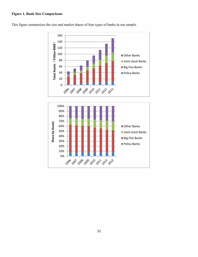
51
Figure 1. Bank Size Comparisons
This figure summarizes the size and market shares of four types of banks in our sample.
0
20
40
60
80
100
120
140
160
Total A
ssets(Trillion RMB)
Other Banks
Joint‐stock Banks
Big Five Banks
Policy Banks
0%
10%
20%
30%
40%
50%
60%
70%
80%
90%
100%
Share by Assets
Other Banks
Joint‐stock Banks
Big Five Banks
Policy Banks
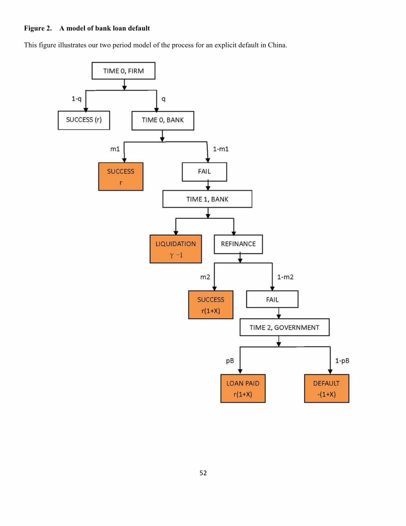
52
Figure 2. A model of bank loan default This figure illustrates our two period model of the process for an explicit default in China.
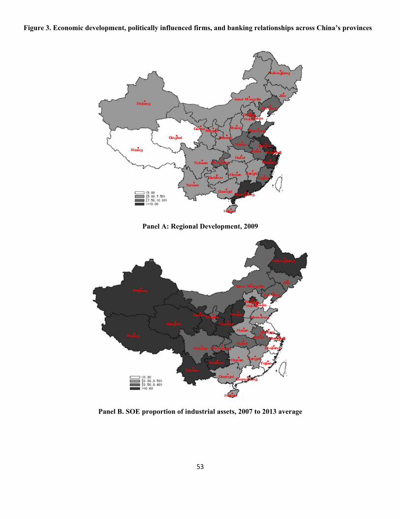
53
Figure 3. Economic development, politically influenced firms, and banking relationships across China’s provinces
Panel A: Regional Development, 2009
Panel B. SOE proportion of industrial assets, 2007 to 2013 average
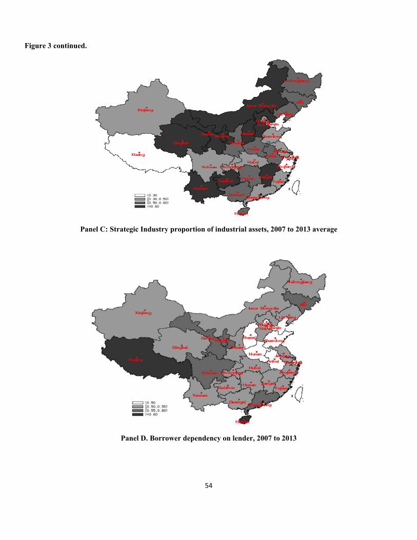
54
Figure 3 continued.
Panel C: Strategic Industry proportion of industrial assets, 2007 to 2013 average
Panel D. Borrower dependency on lender, 2007 to 2013
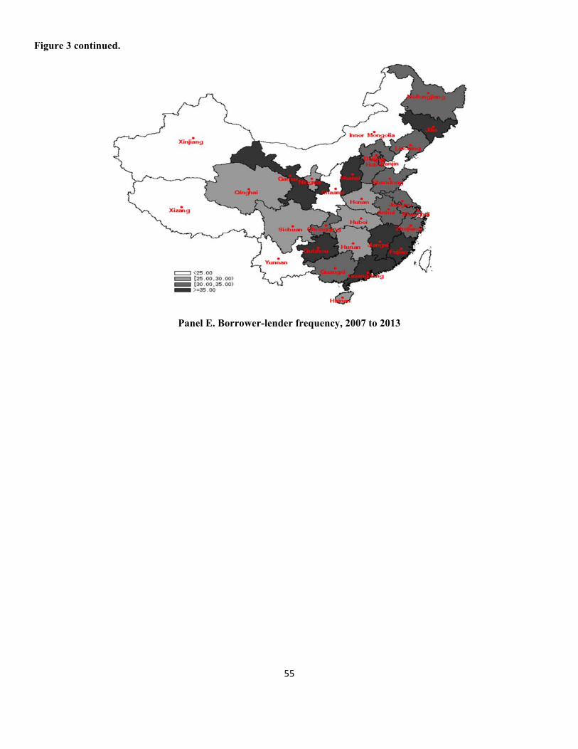
55
Figure 3 continued.
Panel E. Borrower-lender frequency, 2007 to 2013
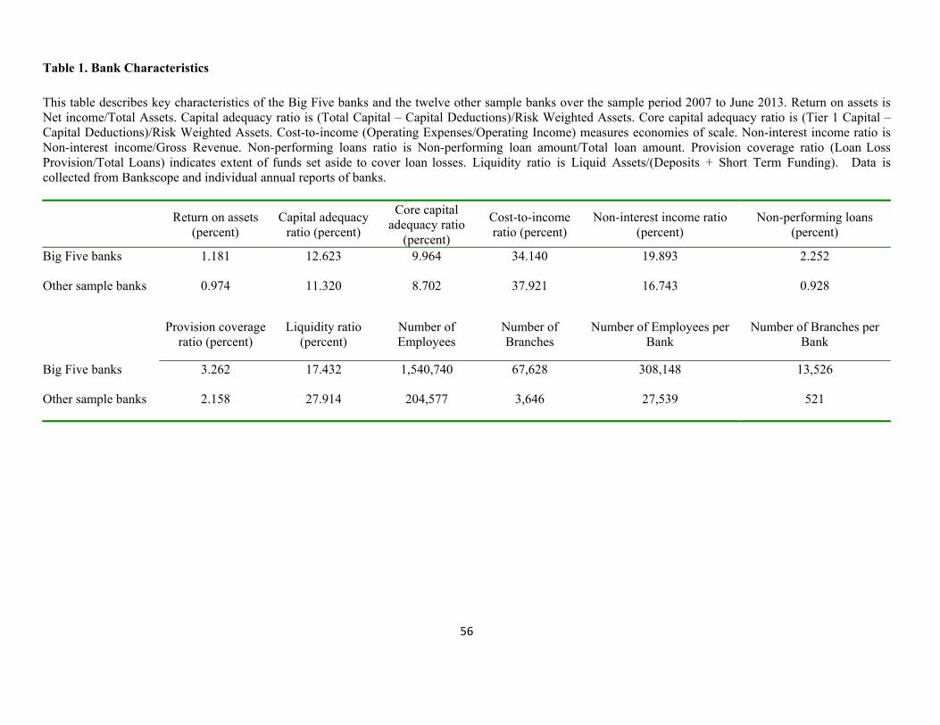
56
Table 1. Bank Characteristics This table describes key characteristics of the Big Five banks and the twelve other sample banks over the sample period 2007 to June 2013. Return on assets is Net income/Total Assets. Capital adequacy ratio is (Total Capital – Capital Deductions)/Risk Weighted Assets. Core capital adequacy ratio is (Tier 1 Capital –Capital Deductions)/Risk Weighted Assets. Cost-to-income (Operating Expenses/Operating Income) measures economies of scale. Non-interest income ratio is Non-interest income/Gross Revenue. Non-performing loans ratio is Non-performing loan amount/Total loan amount. Provision coverage ratio (Loan Loss Provision/Total Loans) indicates extent of funds set aside to cover loan losses. Liquidity ratio is Liquid Assets/(Deposits + Short Term Funding). Data is collected from Bankscope and individual annual reports of banks.
Return on assets (percent)
Capital adequacy ratio (percent)
Core capital adequacy ratio
(percent)
Cost-to-income ratio (percent)
Non-interest income ratio (percent)
Non-performing loans (percent)
Big Five banks 1.181 12.623 9.964 34.140 19.893 2.252
Other sample banks 0.974 11.320 8.702 37.921 16.743 0.928
Provision coverage
ratio (percent) Liquidity ratio
(percent) Number of Employees
Number of Branches
Number of Employees per Bank
Number of Branches per Bank
Big Five banks 3.262 17.432 1,540,740 67,628 308,148 13,526
Other sample banks 2.158 27.914 204,577 3,646 27,539 521
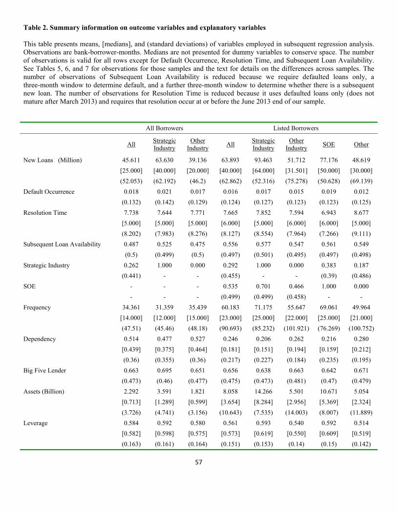
57
Table 2. Summary information on outcome variables and explanatory variables This table presents means, [medians], and (standard deviations) of variables employed in subsequent regression analysis. Observations are bank-borrower-months. Medians are not presented for dummy variables to conserve space. The number of observations is valid for all rows except for Default Occurrence, Resolution Time, and Subsequent Loan Availability. See Tables 5, 6, and 7 for observations for those samples and the text for details on the differences across samples. The number of observations of Subsequent Loan Availability is reduced because we require defaulted loans only, a three-month window to determine default, and a further three-month window to determine whether there is a subsequent new loan. The number of observations for Resolution Time is reduced because it uses defaulted loans only (does not mature after March 2013) and requires that resolution occur at or before the June 2013 end of our sample.
All Borrowers Listed Borrowers
All Strategic Industry
Other Industry
All Strategic Industry
Other Industry
SOE Other
New Loans (Million) 45.611 63.630 39.136 63.893 93.463 51.712 77.176 48.619
[25.000] [40.000] [20.000] [40.000] [64.000] [31.501] [50.000] [30.000]
(52.053) (62.192) (46.2) (62.862) (52.316) (75.278) (50.628) (69.139)
Default Occurrence 0.018 0.021 0.017 0.016 0.017 0.015 0.019 0.012
(0.132) (0.142) (0.129) (0.124) (0.127) (0.123) (0.123) (0.125)
Resolution Time 7.738 7.644 7.771 7.665 7.852 7.594 6.943 8.677
[5.000] [5.000] [5.000] [6.000] [5.000] [6.000] [6.000] [5.000]
(8.202) (7.983) (8.276) (8.127) (8.554) (7.964) (7.266) (9.111)
Subsequent Loan Availability 0.487 0.525 0.475 0.556 0.577 0.547 0.561 0.549
(0.5) (0.499) (0.5) (0.497) (0.501) (0.495) (0.497) (0.498)
Strategic Industry 0.262 1.000 0.000 0.292 1.000 0.000 0.383 0.187
(0.441) - - (0.455) - - (0.39) (0.486)
SOE - - - 0.535 0.701 0.466 1.000 0.000
- - - (0.499) (0.499) (0.458) - -
Frequency 34.361 31.359 35.439 60.183 71.175 55.647 69.061 49.964
[14.000] [12.000] [15.000] [23.000] [25.000] [22.000] [25.000] [21.000]
(47.51) (45.46) (48.18) (90.693) (85.232) (101.921) (76.269) (100.752)
Dependency 0.514 0.477 0.527 0.246 0.206 0.262 0.216 0.280
[0.439] [0.375] [0.464] [0.181] [0.151] [0.194] [0.159] [0.212]
(0.36) (0.355) (0.36) (0.217) (0.227) (0.184) (0.235) (0.195)
Big Five Lender 0.663 0.695 0.651 0.656 0.638 0.663 0.642 0.671
(0.473) (0.46) (0.477) (0.475) (0.473) (0.481) (0.47) (0.479)
Assets (Billion) 2.292 3.591 1.821 8.058 14.266 5.501 10.671 5.054
[0.713] [1.289] [0.599] [3.654] [8.284] [2.956] [5.369] [2.324]
(3.726) (4.741) (3.156) (10.643) (7.535) (14.003) (8.007) (11.889)
Leverage 0.584 0.592 0.580 0.561 0.593 0.540 0.592 0.514
[0.582] [0.598] [0.575] [0.573] [0.619] [0.550] [0.609] [0.519]
(0.163) (0.161) (0.164) (0.151) (0.153) (0.14) (0.15) (0.142)
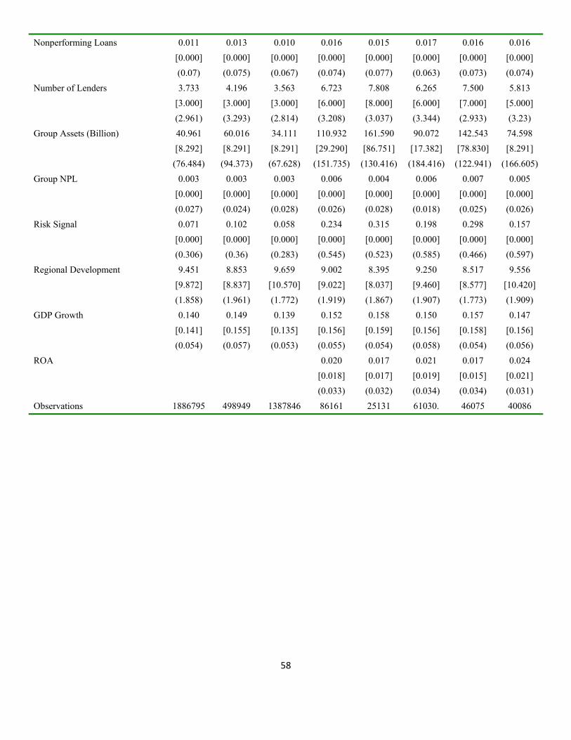
58
Nonperforming Loans 0.011 0.013 0.010 0.016 0.015 0.017 0.016 0.016
[0.000] [0.000] [0.000] [0.000] [0.000] [0.000] [0.000] [0.000]
(0.07) (0.075) (0.067) (0.074) (0.077) (0.063) (0.073) (0.074)
Number of Lenders 3.733 4.196 3.563 6.723 7.808 6.265 7.500 5.813
[3.000] [3.000] [3.000] [6.000] [8.000] [6.000] [7.000] [5.000]
(2.961) (3.293) (2.814) (3.208) (3.037) (3.344) (2.933) (3.23)
Group Assets (Billion) 40.961 60.016 34.111 110.932 161.590 90.072 142.543 74.598
[8.292] [8.291] [8.291] [29.290] [86.751] [17.382] [78.830] [8.291]
(76.484) (94.373) (67.628) (151.735) (130.416) (184.416) (122.941) (166.605)
Group NPL 0.003 0.003 0.003 0.006 0.004 0.006 0.007 0.005
[0.000] [0.000] [0.000] [0.000] [0.000] [0.000] [0.000] [0.000]
(0.027) (0.024) (0.028) (0.026) (0.028) (0.018) (0.025) (0.026)
Risk Signal 0.071 0.102 0.058 0.234 0.315 0.198 0.298 0.157
[0.000] [0.000] [0.000] [0.000] [0.000] [0.000] [0.000] [0.000]
(0.306) (0.36) (0.283) (0.545) (0.523) (0.585) (0.466) (0.597)
Regional Development 9.451 8.853 9.659 9.002 8.395 9.250 8.517 9.556
[9.872] [8.837] [10.570] [9.022] [8.037] [9.460] [8.577] [10.420]
(1.858) (1.961) (1.772) (1.919) (1.867) (1.907) (1.773) (1.909)
GDP Growth 0.140 0.149 0.139 0.152 0.158 0.150 0.157 0.147
[0.141] [0.155] [0.135] [0.156] [0.159] [0.156] [0.158] [0.156]
(0.054) (0.057) (0.053) (0.055) (0.054) (0.058) (0.054) (0.056)
ROA 0.020 0.017 0.021 0.017 0.024
[0.018] [0.017] [0.019] [0.015] [0.021]
(0.033) (0.032) (0.034) (0.034) (0.031)
Observations 1886795 498949 1387846 86161 25131 61030. 46075 40086
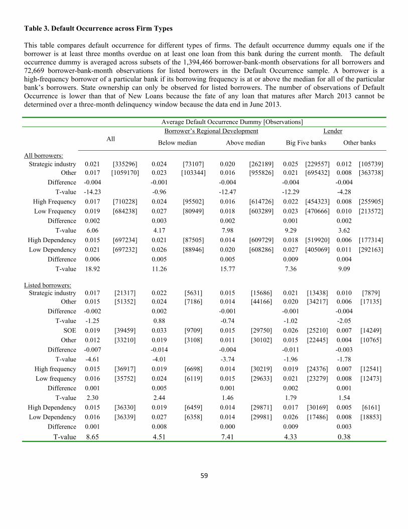
59
Table 3. Default Occurrence across Firm Types This table compares default occurrence for different types of firms. The default occurrence dummy equals one if the borrower is at least three months overdue on at least one loan from this bank during the current month. The default occurrence dummy is averaged across subsets of the 1,394,466 borrower-bank-month observations for all borrowers and 72,669 borrower-bank-month observations for listed borrowers in the Default Occurrence sample. A borrower is a high-frequency borrower of a particular bank if its borrowing frequency is at or above the median for all of the particular bank’s borrowers. State ownership can only be observed for listed borrowers. The number of observations of Default Occurrence is lower than that of New Loans because the fate of any loan that matures after March 2013 cannot be determined over a three-month delinquency window because the data end in June 2013. Average Default Occurrence Dummy [Observations]
All Borrower’s Regional Development Lender
Below median Above median Big Five banks Other banks
All borrowers: Strategic industry 0.021 [335296] 0.024 [73107] 0.020 [262189] 0.025 [229557] 0.012 [105739]
Other 0.017 [1059170] 0.023 [103344] 0.016 [955826] 0.021 [695432] 0.008 [363738]
Difference -0.004 -0.001 -0.004 -0.004 -0.004
T-value -14.23 -0.96 -12.47 -12.29 -4.28
High Frequency 0.017 [710228] 0.024 [95502] 0.016 [614726] 0.022 [454323] 0.008 [255905]
Low Frequency 0.019 [684238] 0.027 [80949] 0.018 [603289] 0.023 [470666] 0.010 [213572]
Difference 0.002 0.003 0.002 0.001 0.002
T-value 6.06 4.17 7.98 9.29 3.62
High Dependency 0.015 [697234] 0.021 [87505] 0.014 [609729] 0.018 [519920] 0.006 [177314]
Low Dependency 0.021 [697232] 0.026 [88946] 0.020 [608286] 0.027 [405069] 0.011 [292163]
Difference 0.006 0.005 0.005 0.009 0.004
T-value 18.92 11.26 15.77 7.36 9.09 Listed borrowers:
Strategic industry 0.017 [21317] 0.022 [5631] 0.015 [15686] 0.021 [13438] 0.010 [7879] Other 0.015 [51352] 0.024 [7186] 0.014 [44166] 0.020 [34217] 0.006 [17135]
Difference -0.002 0.002 -0.001 -0.001 -0.004
T-value -1.25 0.88 -0.74 -1.02 -2.05
SOE 0.019 [39459] 0.033 [9709] 0.015 [29750] 0.026 [25210] 0.007 [14249]
Other 0.012 [33210] 0.019 [3108] 0.011 [30102] 0.015 [22445] 0.004 [10765]
Difference -0.007 -0.014 -0.004 -0.011 -0.003
T-value -4.61 -4.01 -3.74 -1.96 -1.78
High frequency 0.015 [36917] 0.019 [6698] 0.014 [30219] 0.019 [24376] 0.007 [12541]
Low frequency 0.016 [35752] 0.024 [6119] 0.015 [29633] 0.021 [23279] 0.008 [12473]
Difference 0.001 0.005 0.001 0.002 0.001
T-value 2.30 2.44 1.46 1.79 1.54
High Dependency 0.015 [36330] 0.019 [6459] 0.014 [29871] 0.017 [30169] 0.005 [6161]
Low Dependency 0.016 [36339] 0.027 [6358] 0.014 [29981] 0.026 [17486] 0.008 [18853]
Difference 0.001 0.008 0.000 0.009 0.003
T-value 8.65 4.51 7.41 4.33 0.38
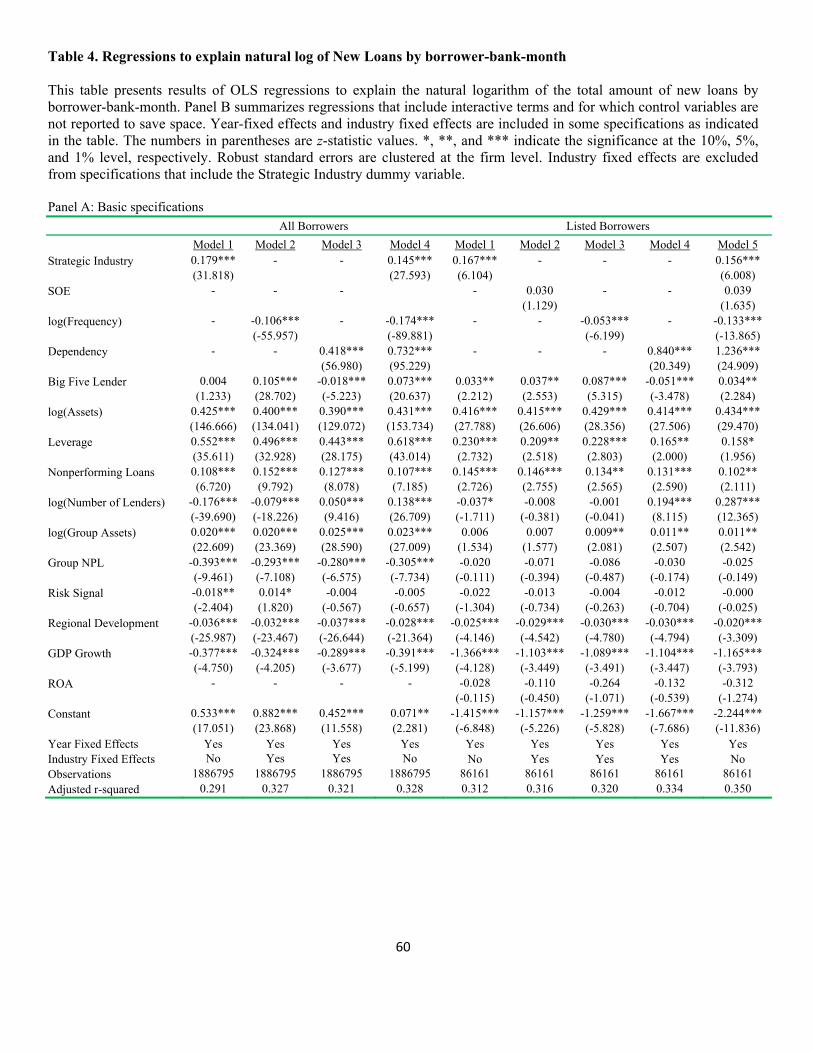
60
Table 4. Regressions to explain natural log of New Loans by borrower-bank-month This table presents results of OLS regressions to explain the natural logarithm of the total amount of new loans by borrower-bank-month. Panel B summarizes regressions that include interactive terms and for which control variables are not reported to save space. Year-fixed effects and industry fixed effects are included in some specifications as indicated in the table. The numbers in parentheses are z-statistic values. *, **, and *** indicate the significance at the 10%, 5%, and 1% level, respectively. Robust standard errors are clustered at the firm level. Industry fixed effects are excluded from specifications that include the Strategic Industry dummy variable. Panel A: Basic specifications
All Borrowers Listed Borrowers
Model 1 Model 2 Model 3 Model 4 Model 1 Model 2 Model 3 Model 4 Model 5 Strategic Industry 0.179*** - - 0.145*** 0.167*** - - - 0.156*** (31.818) (27.593) (6.104) (6.008) SOE - - - - 0.030 - - 0.039 (1.129) (1.635) log(Frequency) - -0.106*** - -0.174*** - - -0.053*** - -0.133*** (-55.957) (-89.881) (-6.199) (-13.865) Dependency - - 0.418*** 0.732*** - - - 0.840*** 1.236*** (56.980) (95.229) (20.349) (24.909) Big Five Lender 0.004 0.105*** -0.018*** 0.073*** 0.033** 0.037** 0.087*** -0.051*** 0.034** (1.233) (28.702) (-5.223) (20.637) (2.212) (2.553) (5.315) (-3.478) (2.284) log(Assets) 0.425*** 0.400*** 0.390*** 0.431*** 0.416*** 0.415*** 0.429*** 0.414*** 0.434*** (146.666) (134.041) (129.072) (153.734) (27.788) (26.606) (28.356) (27.506) (29.470) Leverage 0.552*** 0.496*** 0.443*** 0.618*** 0.230*** 0.209** 0.228*** 0.165** 0.158* (35.611) (32.928) (28.175) (43.014) (2.732) (2.518) (2.803) (2.000) (1.956) Nonperforming Loans 0.108*** 0.152*** 0.127*** 0.107*** 0.145*** 0.146*** 0.134** 0.131*** 0.102** (6.720) (9.792) (8.078) (7.185) (2.726) (2.755) (2.565) (2.590) (2.111) log(Number of Lenders) -0.176*** -0.079*** 0.050*** 0.138*** -0.037* -0.008 -0.001 0.194*** 0.287*** (-39.690) (-18.226) (9.416) (26.709) (-1.711) (-0.381) (-0.041) (8.115) (12.365) log(Group Assets) 0.020*** 0.020*** 0.025*** 0.023*** 0.006 0.007 0.009** 0.011** 0.011** (22.609) (23.369) (28.590) (27.009) (1.534) (1.577) (2.081) (2.507) (2.542) Group NPL -0.393*** -0.293*** -0.280*** -0.305*** -0.020 -0.071 -0.086 -0.030 -0.025 (-9.461) (-7.108) (-6.575) (-7.734) (-0.111) (-0.394) (-0.487) (-0.174) (-0.149) Risk Signal -0.018** 0.014* -0.004 -0.005 -0.022 -0.013 -0.004 -0.012 -0.000 (-2.404) (1.820) (-0.567) (-0.657) (-1.304) (-0.734) (-0.263) (-0.704) (-0.025) Regional Development -0.036*** -0.032*** -0.037*** -0.028*** -0.025*** -0.029*** -0.030*** -0.030*** -0.020*** (-25.987) (-23.467) (-26.644) (-21.364) (-4.146) (-4.542) (-4.780) (-4.794) (-3.309) GDP Growth -0.377*** -0.324*** -0.289*** -0.391*** -1.366*** -1.103*** -1.089*** -1.104*** -1.165*** (-4.750) (-4.205) (-3.677) (-5.199) (-4.128) (-3.449) (-3.491) (-3.447) (-3.793) ROA - - - - -0.028 -0.110 -0.264 -0.132 -0.312 (-0.115) (-0.450) (-1.071) (-0.539) (-1.274) Constant 0.533*** 0.882*** 0.452*** 0.071** -1.415*** -1.157*** -1.259*** -1.667*** -2.244*** (17.051) (23.868) (11.558) (2.281) (-6.848) (-5.226) (-5.828) (-7.686) (-11.836) Year Fixed Effects Yes Yes Yes Yes Yes Yes Yes Yes Yes Industry Fixed Effects No Yes Yes No No Yes Yes Yes No Observations 1886795 1886795 1886795 1886795 86161 86161 86161 86161 86161 Adjusted r-squared 0.291 0.327 0.321 0.328 0.312 0.316 0.320 0.334 0.350
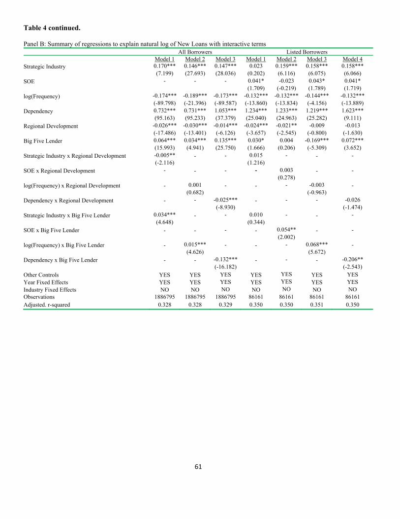
61
Table 4 continued. Panel B: Summary of regressions to explain natural log of New Loans with interactive terms
All Borrowers Listed Borrowers Model 1 Model 2 Model 3 Model 1 Model 2 Model 3 Model 4 Strategic Industry 0.170*** 0.146*** 0.147*** 0.023 0.159*** 0.158*** 0.158*** (7.199) (27.693) (28.036) (0.202) (6.116) (6.075) (6.066) SOE - - - 0.041* -0.023 0.043* 0.041* (1.709) (-0.219) (1.789) (1.719) log(Frequency) -0.174*** -0.189*** -0.173*** -0.132*** -0.132*** -0.144*** -0.132*** (-89.798) (-21.396) (-89.587) (-13.860) (-13.834) (-4.156) (-13.889) Dependency 0.732*** 0.731*** 1.053*** 1.234*** 1.233*** 1.219*** 1.623*** (95.163) (95.233) (37.379) (25.040) (24.963) (25.282) (9.111) Regional Development -0.026*** -0.030*** -0.014*** -0.024*** -0.021** -0.009 -0.013 (-17.486) (-13.401) (-6.126) (-3.657) (-2.545) (-0.800) (-1.630) Big Five Lender 0.064*** 0.034*** 0.135*** 0.030* 0.004 -0.169*** 0.072*** (15.993) (4.941) (25.750) (1.666) (0.206) (-5.309) (3.652) Strategic Industry x Regional Development -0.005** - - 0.015 - - - (-2.116) (1.216) SOE x Regional Development - - - - 0.003 - - (0.278) log(Frequency) x Regional Development - 0.001 - - - -0.003 - (0.682) (-0.963) Dependency x Regional Development - - -0.025*** - - - -0.026 (-8.930) (-1.474) Strategic Industry x Big Five Lender 0.034*** - - 0.010 - - - (4.648) (0.344) SOE x Big Five Lender - - - - 0.054** - - (2.002) log(Frequency) x Big Five Lender - 0.015*** - - - 0.068*** - (4.626) (5.672) Dependency x Big Five Lender - - -0.132*** - - - -0.206** (-16.182) (-2.543) Other Controls YES YES YES YES YES YES YES Year Fixed Effects YES YES YES YES YES YES YES Industry Fixed Effects NO NO NO NO NO NO NO Observations 1886795 1886795 1886795 86161 86161 86161 86161 Adjusted. r-squared 0.328 0.328 0.329 0.350 0.350 0.351 0.350
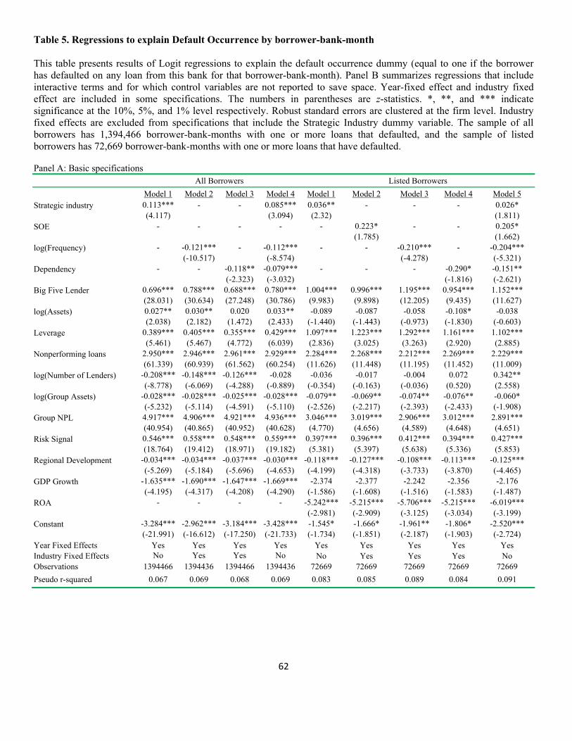
62
Table 5. Regressions to explain Default Occurrence by borrower-bank-month This table presents results of Logit regressions to explain the default occurrence dummy (equal to one if the borrower has defaulted on any loan from this bank for that borrower-bank-month). Panel B summarizes regressions that include interactive terms and for which control variables are not reported to save space. Year-fixed effect and industry fixed effect are included in some specifications. The numbers in parentheses are z-statistics. *, **, and *** indicate significance at the 10%, 5%, and 1% level respectively. Robust standard errors are clustered at the firm level. Industry fixed effects are excluded from specifications that include the Strategic Industry dummy variable. The sample of all borrowers has 1,394,466 borrower-bank-months with one or more loans that defaulted, and the sample of listed borrowers has 72,669 borrower-bank-months with one or more loans that have defaulted. Panel A: Basic specifications All Borrowers Listed Borrowers
Model 1 Model 2 Model 3 Model 4 Model 1 Model 2 Model 3 Model 4 Model 5 Strategic industry 0.113*** - - 0.085*** 0.036** - - - 0.026* (4.117) (3.094) (2.32) (1.811) SOE - - - - - 0.223* - - 0.205* (1.785) (1.662) log(Frequency) - -0.121*** - -0.112*** - - -0.210*** - -0.204*** (-10.517) (-8.574) (-4.278) (-5.321) Dependency - - -0.118** -0.079*** - - - -0.290* -0.151** (-2.323) (-3.032) (-1.816) (-2.621) Big Five Lender 0.696*** 0.788*** 0.688*** 0.780*** 1.004*** 0.996*** 1.195*** 0.954*** 1.152*** (28.031) (30.634) (27.248) (30.786) (9.983) (9.898) (12.205) (9.435) (11.627) log(Assets) 0.027** 0.030** 0.020 0.033** -0.089 -0.087 -0.058 -0.108* -0.038 (2.038) (2.182) (1.472) (2.433) (-1.440) (-1.443) (-0.973) (-1.830) (-0.603) Leverage 0.389*** 0.405*** 0.355*** 0.429*** 1.097*** 1.223*** 1.292*** 1.161*** 1.102*** (5.461) (5.467) (4.772) (6.039) (2.836) (3.025) (3.263) (2.920) (2.885) Nonperforming loans 2.950*** 2.946*** 2.961*** 2.929*** 2.284*** 2.268*** 2.212*** 2.269*** 2.229*** (61.339) (60.939) (61.562) (60.254) (11.626) (11.448) (11.195) (11.452) (11.009) log(Number of Lenders) -0.208*** -0.148*** -0.126*** -0.028 -0.036 -0.017 -0.004 0.072 0.342** (-8.778) (-6.069) (-4.288) (-0.889) (-0.354) (-0.163) (-0.036) (0.520) (2.558) log(Group Assets) -0.028*** -0.028*** -0.025*** -0.028*** -0.079** -0.069** -0.074** -0.076** -0.060* (-5.232) (-5.114) (-4.591) (-5.110) (-2.526) (-2.217) (-2.393) (-2.433) (-1.908) Group NPL 4.917*** 4.906*** 4.921*** 4.936*** 3.046*** 3.019*** 2.906*** 3.012*** 2.891*** (40.954) (40.865) (40.952) (40.628) (4.770) (4.656) (4.589) (4.648) (4.651) Risk Signal 0.546*** 0.558*** 0.548*** 0.559*** 0.397*** 0.396*** 0.412*** 0.394*** 0.427*** (18.764) (19.412) (18.971) (19.182) (5.381) (5.397) (5.638) (5.336) (5.853) Regional Development -0.034*** -0.034*** -0.037*** -0.030*** -0.118*** -0.127*** -0.108*** -0.113*** -0.125*** (-5.269) (-5.184) (-5.696) (-4.653) (-4.199) (-4.318) (-3.733) (-3.870) (-4.465) GDP Growth -1.635*** -1.690*** -1.647*** -1.669*** -2.374 -2.377 -2.242 -2.356 -2.176 (-4.195) (-4.317) (-4.208) (-4.290) (-1.586) (-1.608) (-1.516) (-1.583) (-1.487) ROA - - - - -5.242*** -5.215*** -5.706*** -5.215*** -6.019*** (-2.981) (-2.909) (-3.125) (-3.034) (-3.199) Constant -3.284*** -2.962*** -3.184*** -3.428*** -1.545* -1.666* -1.961** -1.806* -2.520*** (-21.991) (-16.612) (-17.250) (-21.733) (-1.734) (-1.851) (-2.187) (-1.903) (-2.724) Year Fixed Effects Yes Yes Yes Yes Yes Yes Yes Yes Yes Industry Fixed Effects No Yes Yes No No Yes Yes Yes No Observations 1394466 1394436 1394466 1394436 72669 72669 72669 72669 72669
Pseudo r-squared 0.067 0.069 0.068 0.069 0.083 0.085 0.089 0.084 0.091

63
Table 5 continued. Panel B: Summary of regressions to explain default occurrence with interactive terms All Borrowers Listed Borrowers
Model 1 Model 2 Model 3 Model 1 Model 2 Model 3 Model 4 Strategic industry 0.130 0.087*** 0.092*** 0.005* 0.076* 0.083* 0.078* (0.242) (3.172) (3.377) (1.697) (1.761) (1.723) (1.771) SOE - - - 0.210* 0.305* 0.192* 0.199* (1.664) (1.672) (1.669) (1.658) log(Frequency) -0.110*** -0.238*** -0.117*** -0.240*** -0.239*** -0.551*** -0.238*** (-8.525) (-9.222) (-8.364) (-4.623) (-4.547) (-3.411) (-4.591) Dependency -0.074*** -0.070*** -1.041*** -0.153*** -0.158*** -0.146*** -0.612*** (-3.032) (-3.010) (-3.564) (-2.687) (-2.698) (-2.788) (-2.639) Regional Development -0.032*** -0.043*** 0.022* -0.124*** -0.135*** -0.277*** -0.110*** (-4.175) (-3.034) (1.787) (-3.740) (-3.027) (-3.988) (-2.812) Big Five Lender 0.777*** 0.527*** 0.874*** 1.197*** 1.092*** 0.622** 1.118*** (27.308) (9.387) (23.016) (9.575) (7.978) (2.131) (8.072) Strategic industry x Regional Development -0.005** - - -0.003** - - - (-2.363) (-2.049) SOE x Regional Development - - - - -0.017* - - (-1.904) log(Frequency) x Regional Development - 0.005 - - - 0.050** - (0.820) (2.049) Dependency x Regional Development - - 0.089*** - - - 0.050 (5.590) (0.674) Strategic industry x Big Five Lender 0.013* - - 0.077* - - - (1.681) (1.888) SOE x Big Five Lender - - - - 0.074** - - (2.374) log(Frequency) x Big Five Lender - 0.108*** - - - 0.206 - (4.259) (1.634) Dependency x Big Five Lender - - 0.191*** - - - 0.087 (3.015) (0.146) Other Controls YES YES YES YES YES YES YES Year Fixed Effects YES YES YES YES YES YES YES Industry Fixed Effects NO NO NO NO NO NO NO Observations 1394466 1394466 1394466 72669 72669 72669 72669
Pseudo r-squared 0.069 0.069 0.069 0.083 0.083 0.085 0.083
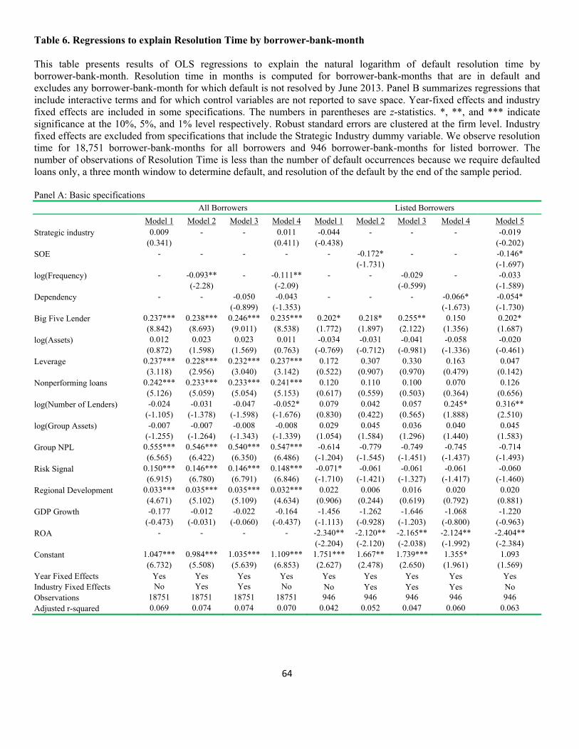
64
Table 6. Regressions to explain Resolution Time by borrower-bank-month This table presents results of OLS regressions to explain the natural logarithm of default resolution time by borrower-bank-month. Resolution time in months is computed for borrower-bank-months that are in default and excludes any borrower-bank-month for which default is not resolved by June 2013. Panel B summarizes regressions that include interactive terms and for which control variables are not reported to save space. Year-fixed effects and industry fixed effects are included in some specifications. The numbers in parentheses are z-statistics. *, **, and *** indicate significance at the 10%, 5%, and 1% level respectively. Robust standard errors are clustered at the firm level. Industry fixed effects are excluded from specifications that include the Strategic Industry dummy variable. We observe resolution time for 18,751 borrower-bank-months for all borrowers and 946 borrower-bank-months for listed borrower. The number of observations of Resolution Time is less than the number of default occurrences because we require defaulted loans only, a three month window to determine default, and resolution of the default by the end of the sample period. Panel A: Basic specifications All Borrowers Listed Borrowers
Model 1 Model 2 Model 3 Model 4 Model 1 Model 2 Model 3 Model 4 Model 5 Strategic industry 0.009 - - 0.011 -0.044 - - - -0.019 (0.341) (0.411) (-0.438) (-0.202) SOE - - - - - -0.172* - - -0.146* (-1.731) (-1.697) log(Frequency) - -0.093** - -0.111** - - -0.029 - -0.033 (-2.28) (-2.09) (-0.599) (-1.589) Dependency - - -0.050 -0.043 - - - -0.066* -0.054* (-0.899) (-1.353) (-1.673) (-1.730) Big Five Lender 0.237*** 0.238*** 0.246*** 0.235*** 0.202* 0.218* 0.255** 0.150 0.202* (8.842) (8.693) (9.011) (8.538) (1.772) (1.897) (2.122) (1.356) (1.687) log(Assets) 0.012 0.023 0.023 0.011 -0.034 -0.031 -0.041 -0.058 -0.020 (0.872) (1.598) (1.569) (0.763) (-0.769) (-0.712) (-0.981) (-1.336) (-0.461) Leverage 0.237*** 0.228*** 0.232*** 0.237*** 0.172 0.307 0.330 0.163 0.047 (3.118) (2.956) (3.040) (3.142) (0.522) (0.907) (0.970) (0.479) (0.142) Nonperforming loans 0.242*** 0.233*** 0.233*** 0.241*** 0.120 0.110 0.100 0.070 0.126 (5.126) (5.059) (5.054) (5.153) (0.617) (0.559) (0.503) (0.364) (0.656) log(Number of Lenders) -0.024 -0.031 -0.047 -0.052* 0.079 0.042 0.057 0.245* 0.316** (-1.105) (-1.378) (-1.598) (-1.676) (0.830) (0.422) (0.565) (1.888) (2.510) log(Group Assets) -0.007 -0.007 -0.008 -0.008 0.029 0.045 0.036 0.040 0.045 (-1.255) (-1.264) (-1.343) (-1.339) (1.054) (1.584) (1.296) (1.440) (1.583) Group NPL 0.555*** 0.546*** 0.540*** 0.547*** -0.614 -0.779 -0.749 -0.745 -0.714 (6.565) (6.422) (6.350) (6.486) (-1.204) (-1.545) (-1.451) (-1.437) (-1.493) Risk Signal 0.150*** 0.146*** 0.146*** 0.148*** -0.071* -0.061 -0.061 -0.061 -0.060 (6.915) (6.780) (6.791) (6.846) (-1.710) (-1.421) (-1.327) (-1.417) (-1.460) Regional Development 0.033*** 0.035*** 0.035*** 0.032*** 0.022 0.006 0.016 0.020 0.020 (4.671) (5.102) (5.109) (4.634) (0.906) (0.244) (0.619) (0.792) (0.881) GDP Growth -0.177 -0.012 -0.022 -0.164 -1.456 -1.262 -1.646 -1.068 -1.220 (-0.473) (-0.031) (-0.060) (-0.437) (-1.113) (-0.928) (-1.203) (-0.800) (-0.963) ROA - - - - -2.340** -2.120** -2.165** -2.124** -2.404** (-2.204) (-2.120) (-2.038) (-1.992) (-2.384) Constant 1.047*** 0.984*** 1.035*** 1.109*** 1.751*** 1.667** 1.739*** 1.355* 1.093 (6.732) (5.508) (5.639) (6.853) (2.627) (2.478) (2.650) (1.961) (1.569) Year Fixed Effects Yes Yes Yes Yes Yes Yes Yes Yes Yes Industry Fixed Effects No Yes Yes No No Yes Yes Yes No Observations 18751 18751 18751 18751 946 946 946 946 946 Adjusted r-squared 0.069 0.074 0.074 0.070 0.042 0.052 0.047 0.060 0.063
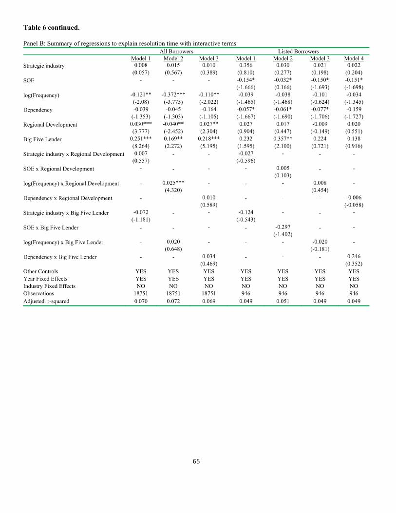
65
Table 6 continued. Panel B: Summary of regressions to explain resolution time with interactive terms All Borrowers Listed Borrowers Model 1 Model 2 Model 3 Model 1 Model 2 Model 3 Model 4 Strategic industry 0.008 0.015 0.010 0.356 0.030 0.021 0.022 (0.057) (0.567) (0.389) (0.810) (0.277) (0.198) (0.204) SOE - - - -0.154* -0.032* -0.150* -0.151* (-1.666) (0.166) (-1.693) (-1.698) log(Frequency) -0.121** -0.372*** -0.110** -0.039 -0.038 -0.101 -0.034 (-2.08) (-3.775) (-2.022) (-1.465) (-1.468) (-0.624) (-1.345) Dependency -0.039 -0.045 -0.164 -0.057* -0.061* -0.077* -0.159 (-1.353) (-1.303) (-1.105) (-1.667) (-1.690) (-1.706) (-1.727) Regional Development 0.030*** -0.040** 0.027** 0.027 0.017 -0.009 0.020 (3.777) (-2.452) (2.304) (0.904) (0.447) (-0.149) (0.551) Big Five Lender 0.251*** 0.169** 0.218*** 0.232 0.357** 0.224 0.138 (8.264) (2.272) (5.195) (1.595) (2.100) (0.721) (0.916) Strategic industry x Regional Development 0.007 - - -0.027 - - - (0.557) (-0.596) SOE x Regional Development - - - - 0.005 - - (0.103) log(Frequency) x Regional Development - 0.025*** - - - 0.008 - (4.320) (0.454) Dependency x Regional Development - - 0.010 - - - -0.006 (0.589) (-0.058) Strategic industry x Big Five Lender -0.072 - - -0.124 - - - (-1.181) (-0.543) SOE x Big Five Lender - - - - -0.297 - - (-1.402) log(Frequency) x Big Five Lender - 0.020 - - - -0.020 - (0.648) (-0.181) Dependency x Big Five Lender - - 0.034 - - - 0.246 (0.469) (0.352) Other Controls YES YES YES YES YES YES YES Year Fixed Effects YES YES YES YES YES YES YES Industry Fixed Effects NO NO NO NO NO NO NO Observations 18751 18751 18751 946 946 946 946 Adjusted. r-squared 0.070 0.072 0.069 0.049 0.051 0.049 0.049
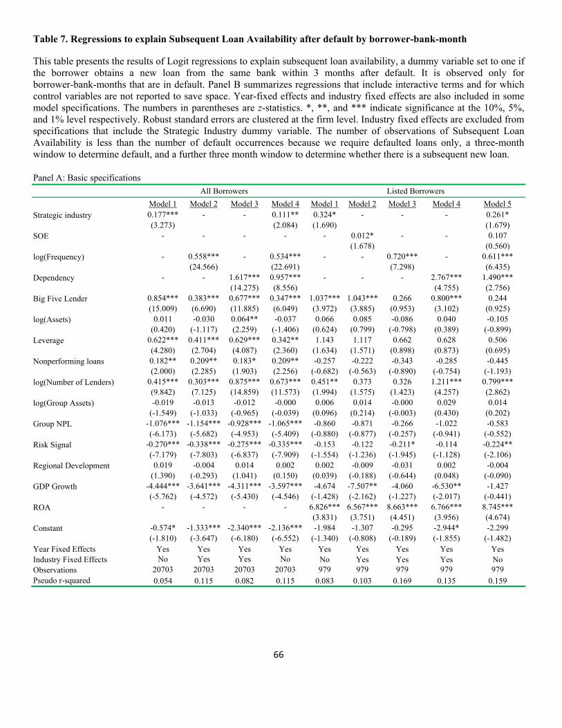
66
Table 7. Regressions to explain Subsequent Loan Availability after default by borrower-bank-month This table presents the results of Logit regressions to explain subsequent loan availability, a dummy variable set to one if the borrower obtains a new loan from the same bank within 3 months after default. It is observed only for borrower-bank-months that are in default. Panel B summarizes regressions that include interactive terms and for which control variables are not reported to save space. Year-fixed effects and industry fixed effects are also included in some model specifications. The numbers in parentheses are z-statistics. *, **, and *** indicate significance at the 10%, 5%, and 1% level respectively. Robust standard errors are clustered at the firm level. Industry fixed effects are excluded from specifications that include the Strategic Industry dummy variable. The number of observations of Subsequent Loan Availability is less than the number of default occurrences because we require defaulted loans only, a three-month window to determine default, and a further three month window to determine whether there is a subsequent new loan. Panel A: Basic specifications
All Borrowers Listed Borrowers
Model 1 Model 2 Model 3 Model 4 Model 1 Model 2 Model 3 Model 4 Model 5 Strategic industry 0.177*** - - 0.111** 0.324* - - - 0.261* (3.273) (2.084) (1.690) (1.679) SOE - - - - - 0.012* - - 0.107 (1.678) (0.560) log(Frequency) - 0.558*** - 0.534*** - - 0.720*** - 0.611*** (24.566) (22.691) (7.298) (6.435) Dependency - - 1.617*** 0.957*** - - - 2.767*** 1.490*** (14.275) (8.556) (4.755) (2.756) Big Five Lender 0.854*** 0.383*** 0.677*** 0.347*** 1.037*** 1.043*** 0.266 0.800*** 0.244 (15.009) (6.690) (11.885) (6.049) (3.972) (3.885) (0.953) (3.102) (0.925) log(Assets) 0.011 -0.030 0.064** -0.037 0.066 0.085 -0.086 0.040 -0.105 (0.420) (-1.117) (2.259) (-1.406) (0.624) (0.799) (-0.798) (0.389) (-0.899) Leverage 0.622*** 0.411*** 0.629*** 0.342** 1.143 1.117 0.662 0.628 0.506 (4.280) (2.704) (4.087) (2.360) (1.634) (1.571) (0.898) (0.873) (0.695) Nonperforming loans 0.182** 0.209** 0.183* 0.209** -0.257 -0.222 -0.343 -0.285 -0.445 (2.000) (2.285) (1.903) (2.256) (-0.682) (-0.563) (-0.890) (-0.754) (-1.193) log(Number of Lenders) 0.415*** 0.303*** 0.875*** 0.673*** 0.451** 0.373 0.326 1.211*** 0.799*** (9.842) (7.125) (14.859) (11.573) (1.994) (1.575) (1.423) (4.257) (2.862) log(Group Assets) -0.019 -0.013 -0.012 -0.000 0.006 0.014 -0.000 0.029 0.014 (-1.549) (-1.033) (-0.965) (-0.039) (0.096) (0.214) (-0.003) (0.430) (0.202) Group NPL -1.076*** -1.154*** -0.928*** -1.065*** -0.860 -0.871 -0.266 -1.022 -0.583 (-6.173) (-5.682) (-4.953) (-5.409) (-0.880) (-0.877) (-0.257) (-0.941) (-0.552) Risk Signal -0.270*** -0.338*** -0.275*** -0.335*** -0.153 -0.122 -0.211* -0.114 -0.224** (-7.179) (-7.803) (-6.837) (-7.909) (-1.554) (-1.236) (-1.945) (-1.128) (-2.106) Regional Development 0.019 -0.004 0.014 0.002 0.002 -0.009 -0.031 0.002 -0.004 (1.390) (-0.293) (1.041) (0.150) (0.039) (-0.188) (-0.644) (0.048) (-0.090) GDP Growth -4.444*** -3.641*** -4.311*** -3.597*** -4.674 -7.507** -4.060 -6.530** -1.427 (-5.762) (-4.572) (-5.430) (-4.546) (-1.428) (-2.162) (-1.227) (-2.017) (-0.441) ROA - - - - 6.826*** 6.567*** 8.663*** 6.766*** 8.745*** (3.831) (3.751) (4.451) (3.956) (4.674) Constant -0.574* -1.333*** -2.340*** -2.136*** -1.984 -1.307 -0.295 -2.944* -2.299 (-1.810) (-3.647) (-6.180) (-6.552) (-1.340) (-0.808) (-0.189) (-1.855) (-1.482) Year Fixed Effects Yes Yes Yes Yes Yes Yes Yes Yes Yes Industry Fixed Effects No Yes Yes No No Yes Yes Yes No Observations 20703 20703 20703 20703 979 979 979 979 979 Pseudo r-squared 0.054 0.115 0.082 0.115 0.083 0.103 0.169 0.135 0.159
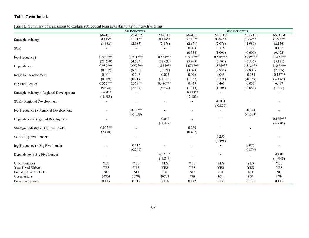
67
Table 7 continued. Panel B: Summary of regressions to explain subsequent loan availability with interactive terms All Borrowers Listed Borrowers Model 1 Model 2 Model 3 Model 1 Model 2 Model 3 Model 4 Strategic industry 0.118* 0.111** 0.116** 2.215** 0.294** 0.258** 0.296** (1.662) (2.085) (2.176) (2.671) (2.076) (1.989) (2.156) SOE - - - 0.068 0.716 0.121 0.132 (0.334) (1.005) (0.601) (0.653) log(Frequency) 0.534*** 0.571*** 0.534*** 0.531*** 0.536*** 0.909*** 0.505*** (22.698) (4.580) (22.693) (5.493) (5.501) (6.535) (5.121) Dependency 0.957*** 0.957*** 1.154*** 1.671*** 1.565*** 1.512*** 3.858*** (8.562) (8.551) (8.579) (3.073) (2.930) (2.803) (2.668) Regional Development 0.001 0.007 -0.025 0.076 0.049 -0.134 -0.157** (0.089) (0.219) (-1.172) (1.337) (0.728) (-0.953) (-2.069) Big Five Lender 0.352*** 0.379** 0.480*** 0.439 0.460 0.050 0.487 (5.498) (2.400) (5.532) (1.318) (1.108) (0.082) (1.446) Strategic industry x Regional Development -0.002* - - -0.233** - - - (-1.885) (-2.423) SOE x Regional Development - - - - -0.084 - - (-0.870) log(Frequency) x Regional Development - -0.002** - - - -0.044 - (-2.159) (-1.009) Dependency x Regional Development - - -0.047 - - - -0.185*** (-1.487) (-2.605) Strategic industry x Big Five Lender 0.022** - - 0.260 - - - (2.170) (0.487) SOE x Big Five Lender - - - - 0.253 - - (0.496) log(Frequency) x Big Five Lender -- 0.012 - - - 0.075 - (0.203) (0.374) Dependency x Big Five Lender - - -0.273* - - - -1.009 (-1.847) (-0.940) Other Controls YES YES YES YES YES YES YES Year Fixed Effects YES YES YES YES YES YES YES Industry Fixed Effects NO NO NO NO NO NO NO Observations 20703 20703 20703 979 979 979 979 Pseudo r-squared 0.115 0.115 0.116 0.142 0.137 0.137 0.145
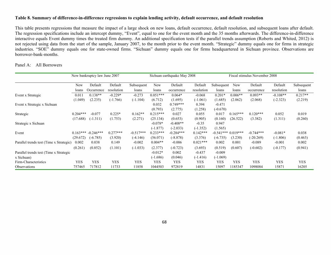
68
Table 8. Summary of difference-in-difference regressions to explain lending activity, default occurrence, and default resolution
This table presents regressions that measure the impact of a large shock on new loans, default occurrence, default resolution, and subsequent loans after default. The regression specifications include an intercept dummy, “Event”, equal to one for the event month and the 35 months afterwards. The difference-in-difference interactive equals Event dummy times the treated firm dummy. An additional specification tests if the parallel trends assumption (Roberts and Whited, 2012) is not rejected using data from the start of the sample, January 2007, to the month prior to the event month. “Strategic” dummy equals one for firms in strategic industries. “SOE” dummy equals one for state-owned firms. “Sichuan” dummy equals one for firms headquartered in Sichuan province. Observations are borrower-bank-months.
Panel A: All Borrowers
New bankruptcy law June 2007 Sichuan earthquake May 2008 Fiscal stimulus November 2008
New loans
Default Occurrence
Default resolution
Subsequent loans
New loans
Default occurrence
Default resolution
Subsequentloans
New loans
Default occurrence
Default resolution
Subsequent loans
Event x Strategic 0.011 0.138** -0.229* -0.273 0.051*** 0.064* -0.068 0.201* 0.006** 0.093** -0.108** 0.217** (1.049) (2.235) (-1.766) (-1.104) (6.712) (1.695) (-1.061) (1.685) (2.062) (2.068) (-2.323) (2.219) Event x Strategic x Sichuan 0.032 0.749*** 0.394 -0.471 (0.793) (2.775) (1.258) (-0.670) Strategic 0.204*** -0.077 0.225* 0.162** 0.215*** 0.027 0.055 0.017 0.165*** 0.120*** 0.052 0.019 (17.688) (-1.311) (1.753) (2.271) (25.134) (0.653) (0.905) (0.160) (26.522) (3.382) (1.311) (0.260) Strategic x Sichuan -0.078* -0.408** -0.35 0.947 (-1.877) (-2.033) (-1.352) (1.565) Event 0.163*** -0.246*** 0.277*** -0.517*** 0.233*** -0.284*** 0.142*** -0.541*** 0.019*** -0.744*** -0.081* 0.038 (29.672) (-6.785) (3.920) (-4.146) (56.071) (-8.878) (3.376) (-6.735) (3.230) (-20.269) (-1.806) (0.463) Parallel trends test (Time x Strategic) 0.002 0.038 0.149 -0.002 0.004** -0.006 0.021*** 0.002 0.001 -0.089 -0.001 0.002
(0.261) (0.852) (1.101) (-1.033) (2.377) (-0.723) (3.693) (0.519) (0.607) (-0.602) (-0.177) (0.941) Parallel trends test (Time x Strategic x Sichuan)
-0.012* 0.002 -0.437 -0.009 (-1.686) (0.046) (-1.416) (-1.069)
Firm-Characteristics YES YES YES YES YES YES YES YES YES YES YES YES Observations 757465 717812 11733 11858 1044503 972819 14831 15097 1185347 1098084 15871 16205
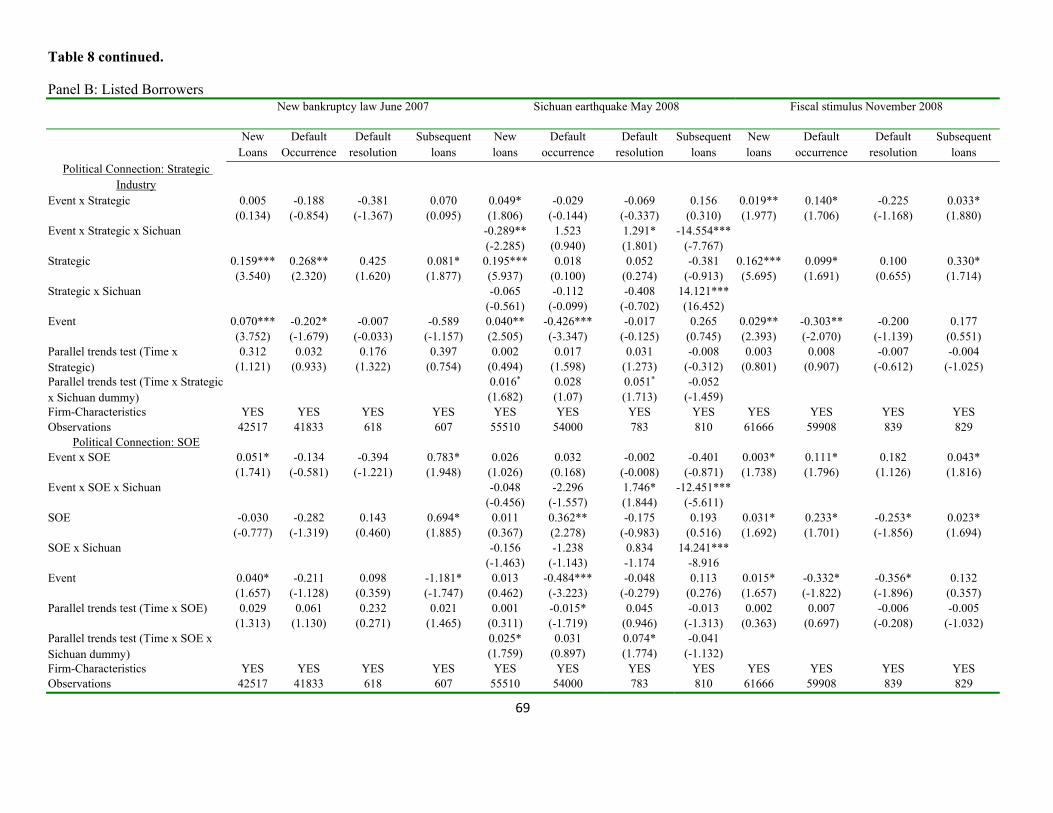
69
Table 8 continued.
Panel B: Listed Borrowers New bankruptcy law June 2007 Sichuan earthquake May 2008 Fiscal stimulus November 2008
New Loans
Default Occurrence
Default resolution
Subsequent loans
New loans
Default occurrence
Default resolution
Subsequentloans
New loans
Default occurrence
Default resolution
Subsequent loans
Political Connection: Strategic Industry
Event x Strategic 0.005 -0.188 -0.381 0.070 0.049* -0.029 -0.069 0.156 0.019** 0.140* -0.225 0.033* (0.134) (-0.854) (-1.367) (0.095) (1.806) (-0.144) (-0.337) (0.310) (1.977) (1.706) (-1.168) (1.880) Event x Strategic x Sichuan -0.289** 1.523 1.291* -14.554*** (-2.285) (0.940) (1.801) (-7.767) Strategic 0.159*** 0.268** 0.425 0.081* 0.195*** 0.018 0.052 -0.381 0.162*** 0.099* 0.100 0.330* (3.540) (2.320) (1.620) (1.877) (5.937) (0.100) (0.274) (-0.913) (5.695) (1.691) (0.655) (1.714) Strategic x Sichuan -0.065 -0.112 -0.408 14.121*** (-0.561) (-0.099) (-0.702) (16.452) Event 0.070*** -0.202* -0.007 -0.589 0.040** -0.426*** -0.017 0.265 0.029** -0.303** -0.200 0.177 (3.752) (-1.679) (-0.033) (-1.157) (2.505) (-3.347) (-0.125) (0.745) (2.393) (-2.070) (-1.139) (0.551) Parallel trends test (Time x Strategic)
0.312 0.032 0.176 0.397 0.002 0.017 0.031 -0.008 0.003 0.008 -0.007 -0.004 (1.121) (0.933) (1.322) (0.754) (0.494) (1.598) (1.273) (-0.312) (0.801) (0.907) (-0.612) (-1.025)
Parallel trends test (Time x Strategic x Sichuan dummy)
0.016* 0.028 0.051* -0.052 (1.682) (1.07) (1.713) (-1.459)
Firm-Characteristics YES YES YES YES YES YES YES YES YES YES YES YES Observations 42517 41833 618 607 55510 54000 783 810 61666 59908 839 829
Political Connection: SOE Event x SOE 0.051* -0.134 -0.394 0.783* 0.026 0.032 -0.002 -0.401 0.003* 0.111* 0.182 0.043* (1.741) (-0.581) (-1.221) (1.948) (1.026) (0.168) (-0.008) (-0.871) (1.738) (1.796) (1.126) (1.816) Event x SOE x Sichuan -0.048 -2.296 1.746* -12.451*** (-0.456) (-1.557) (1.844) (-5.611) SOE -0.030 -0.282 0.143 0.694* 0.011 0.362** -0.175 0.193 0.031* 0.233* -0.253* 0.023* (-0.777) (-1.319) (0.460) (1.885) (0.367) (2.278) (-0.983) (0.516) (1.692) (1.701) (-1.856) (1.694) SOE x Sichuan -0.156 -1.238 0.834 14.241*** (-1.463) (-1.143) -1.174 -8.916 Event 0.040* -0.211 0.098 -1.181* 0.013 -0.484*** -0.048 0.113 0.015* -0.332* -0.356* 0.132 (1.657) (-1.128) (0.359) (-1.747) (0.462) (-3.223) (-0.279) (0.276) (1.657) (-1.822) (-1.896) (0.357) Parallel trends test (Time x SOE) 0.029 0.061 0.232 0.021 0.001 -0.015* 0.045 -0.013 0.002 0.007 -0.006 -0.005 (1.313) (1.130) (0.271) (1.465) (0.311) (-1.719) (0.946) (-1.313) (0.363) (0.697) (-0.208) (-1.032) Parallel trends test (Time x SOE x Sichuan dummy)
0.025* 0.031 0.074* -0.041 (1.759) (0.897) (1.774) (-1.132)
Firm-Characteristics YES YES YES YES YES YES YES YES YES YES YES YES Observations 42517 41833 618 607 55510 54000 783 810 61666 59908 839 829
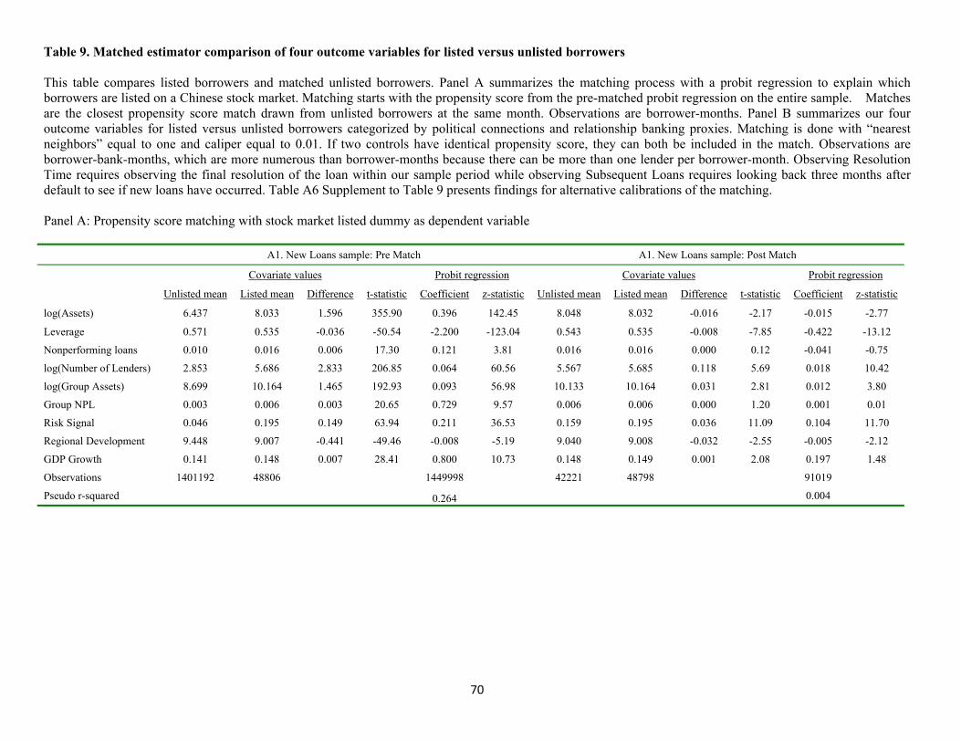
70
Table 9. Matched estimator comparison of four outcome variables for listed versus unlisted borrowers This table compares listed borrowers and matched unlisted borrowers. Panel A summarizes the matching process with a probit regression to explain which borrowers are listed on a Chinese stock market. Matching starts with the propensity score from the pre-matched probit regression on the entire sample. Matches are the closest propensity score match drawn from unlisted borrowers at the same month. Observations are borrower-months. Panel B summarizes our four outcome variables for listed versus unlisted borrowers categorized by political connections and relationship banking proxies. Matching is done with “nearest neighbors” equal to one and caliper equal to 0.01. If two controls have identical propensity score, they can both be included in the match. Observations are borrower-bank-months, which are more numerous than borrower-months because there can be more than one lender per borrower-month. Observing Resolution Time requires observing the final resolution of the loan within our sample period while observing Subsequent Loans requires looking back three months after default to see if new loans have occurred. Table A6 Supplement to Table 9 presents findings for alternative calibrations of the matching. Panel A: Propensity score matching with stock market listed dummy as dependent variable A1. New Loans sample: Pre Match A1. New Loans sample: Post Match
Covariate values Probit regression Covariate values Probit regression
Unlisted mean Listed mean Difference t-statistic Coefficient z-statistic Unlisted mean Listed mean Difference t-statistic Coefficient z-statistic
log(Assets) 6.437 8.033 1.596 355.90 0.396 142.45 8.048 8.032 -0.016 -2.17 -0.015 -2.77
Leverage 0.571 0.535 -0.036 -50.54 -2.200 -123.04 0.543 0.535 -0.008 -7.85 -0.422 -13.12
Nonperforming loans 0.010 0.016 0.006 17.30 0.121 3.81 0.016 0.016 0.000 0.12 -0.041 -0.75
log(Number of Lenders) 2.853 5.686 2.833 206.85 0.064 60.56 5.567 5.685 0.118 5.69 0.018 10.42
log(Group Assets) 8.699 10.164 1.465 192.93 0.093 56.98 10.133 10.164 0.031 2.81 0.012 3.80
Group NPL 0.003 0.006 0.003 20.65 0.729 9.57 0.006 0.006 0.000 1.20 0.001 0.01
Risk Signal 0.046 0.195 0.149 63.94 0.211 36.53 0.159 0.195 0.036 11.09 0.104 11.70
Regional Development 9.448 9.007 -0.441 -49.46 -0.008 -5.19 9.040 9.008 -0.032 -2.55 -0.005 -2.12
GDP Growth 0.141 0.148 0.007 28.41 0.800 10.73 0.148 0.149 0.001 2.08 0.197 1.48
Observations 1401192 48806 1449998 42221 48798 91019
Pseudo r-squared 0.264 0.004
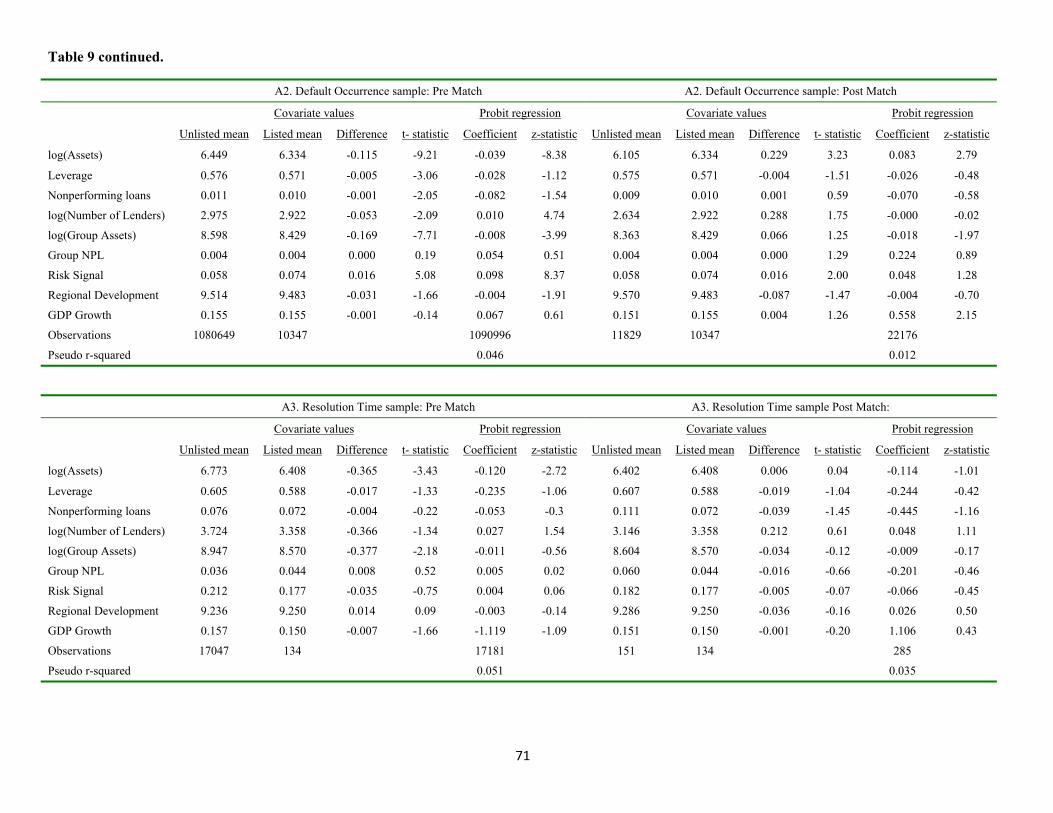
71
Table 9 continued.
A2. Default Occurrence sample: Pre Match A2. Default Occurrence sample: Post Match
Covariate values Probit regression Covariate values Probit regression
Unlisted mean Listed mean Difference t- statistic Coefficient z-statistic Unlisted mean Listed mean Difference t- statistic Coefficient z-statistic
log(Assets) 6.449 6.334 -0.115 -9.21 -0.039 -8.38 6.105 6.334 0.229 3.23 0.083 2.79
Leverage 0.576 0.571 -0.005 -3.06 -0.028 -1.12 0.575 0.571 -0.004 -1.51 -0.026 -0.48
Nonperforming loans 0.011 0.010 -0.001 -2.05 -0.082 -1.54 0.009 0.010 0.001 0.59 -0.070 -0.58
log(Number of Lenders) 2.975 2.922 -0.053 -2.09 0.010 4.74 2.634 2.922 0.288 1.75 -0.000 -0.02
log(Group Assets) 8.598 8.429 -0.169 -7.71 -0.008 -3.99 8.363 8.429 0.066 1.25 -0.018 -1.97
Group NPL 0.004 0.004 0.000 0.19 0.054 0.51 0.004 0.004 0.000 1.29 0.224 0.89
Risk Signal 0.058 0.074 0.016 5.08 0.098 8.37 0.058 0.074 0.016 2.00 0.048 1.28
Regional Development 9.514 9.483 -0.031 -1.66 -0.004 -1.91 9.570 9.483 -0.087 -1.47 -0.004 -0.70
GDP Growth 0.155 0.155 -0.001 -0.14 0.067 0.61 0.151 0.155 0.004 1.26 0.558 2.15
Observations 1080649 10347 1090996 11829 10347 22176
Pseudo r-squared 0.046 0.012
A3. Resolution Time sample: Pre Match A3. Resolution Time sample Post Match:
Covariate values Probit regression Covariate values Probit regression
Unlisted mean Listed mean Difference t- statistic Coefficient z-statistic Unlisted mean Listed mean Difference t- statistic Coefficient z-statistic
log(Assets) 6.773 6.408 -0.365 -3.43 -0.120 -2.72 6.402 6.408 0.006 0.04 -0.114 -1.01
Leverage 0.605 0.588 -0.017 -1.33 -0.235 -1.06 0.607 0.588 -0.019 -1.04 -0.244 -0.42
Nonperforming loans 0.076 0.072 -0.004 -0.22 -0.053 -0.3 0.111 0.072 -0.039 -1.45 -0.445 -1.16
log(Number of Lenders) 3.724 3.358 -0.366 -1.34 0.027 1.54 3.146 3.358 0.212 0.61 0.048 1.11
log(Group Assets) 8.947 8.570 -0.377 -2.18 -0.011 -0.56 8.604 8.570 -0.034 -0.12 -0.009 -0.17
Group NPL 0.036 0.044 0.008 0.52 0.005 0.02 0.060 0.044 -0.016 -0.66 -0.201 -0.46
Risk Signal 0.212 0.177 -0.035 -0.75 0.004 0.06 0.182 0.177 -0.005 -0.07 -0.066 -0.45
Regional Development 9.236 9.250 0.014 0.09 -0.003 -0.14 9.286 9.250 -0.036 -0.16 0.026 0.50
GDP Growth 0.157 0.150 -0.007 -1.66 -1.119 -1.09 0.151 0.150 -0.001 -0.20 1.106 0.43
Observations 17047 134 17181 151 134 285
Pseudo r-squared 0.051 0.035
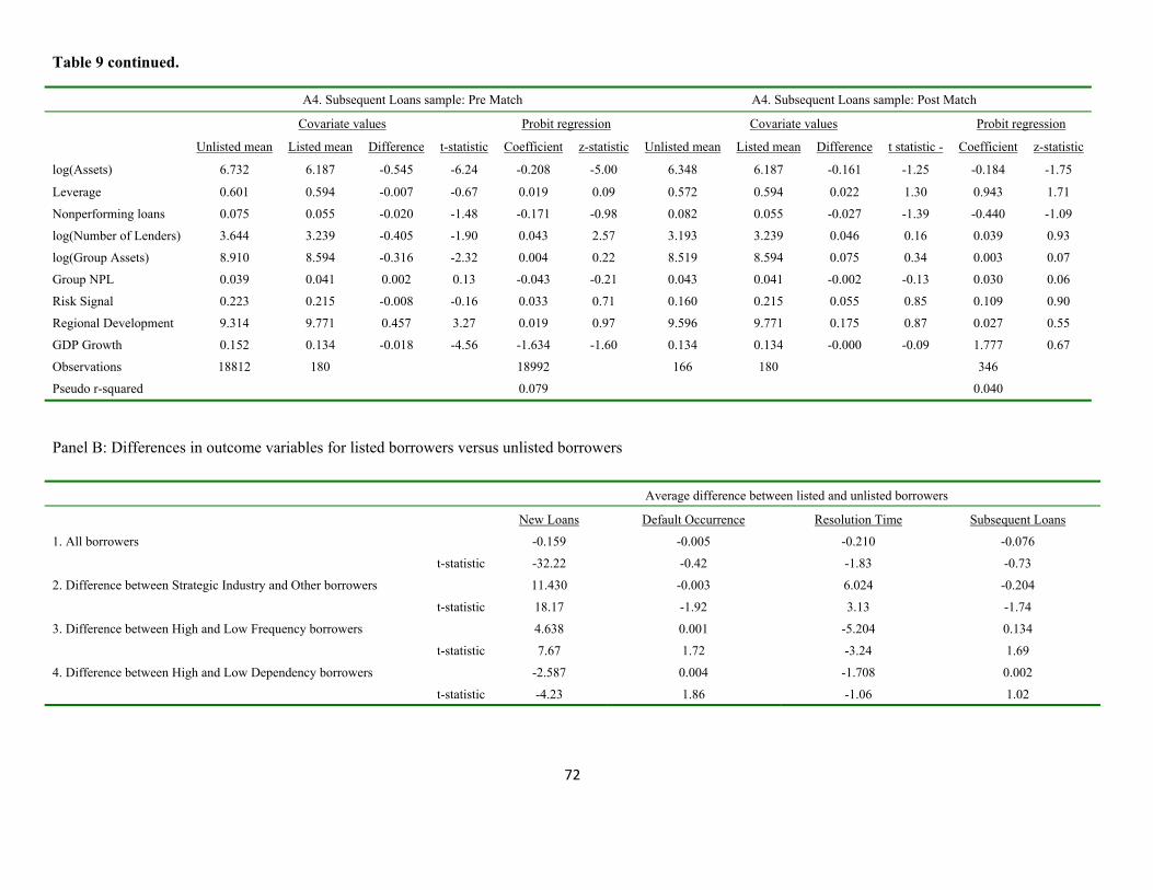
72
Table 9 continued.
A4. Subsequent Loans sample: Pre Match A4. Subsequent Loans sample: Post Match
Covariate values Probit regression Covariate values Probit regression
Unlisted mean Listed mean Difference t-statistic Coefficient z-statistic Unlisted mean Listed mean Difference t statistic - Coefficient z-statistic
log(Assets) 6.732 6.187 -0.545 -6.24 -0.208 -5.00 6.348 6.187 -0.161 -1.25 -0.184 -1.75
Leverage 0.601 0.594 -0.007 -0.67 0.019 0.09 0.572 0.594 0.022 1.30 0.943 1.71
Nonperforming loans 0.075 0.055 -0.020 -1.48 -0.171 -0.98 0.082 0.055 -0.027 -1.39 -0.440 -1.09
log(Number of Lenders) 3.644 3.239 -0.405 -1.90 0.043 2.57 3.193 3.239 0.046 0.16 0.039 0.93
log(Group Assets) 8.910 8.594 -0.316 -2.32 0.004 0.22 8.519 8.594 0.075 0.34 0.003 0.07
Group NPL 0.039 0.041 0.002 0.13 -0.043 -0.21 0.043 0.041 -0.002 -0.13 0.030 0.06
Risk Signal 0.223 0.215 -0.008 -0.16 0.033 0.71 0.160 0.215 0.055 0.85 0.109 0.90
Regional Development 9.314 9.771 0.457 3.27 0.019 0.97 9.596 9.771 0.175 0.87 0.027 0.55
GDP Growth 0.152 0.134 -0.018 -4.56 -1.634 -1.60 0.134 0.134 -0.000 -0.09 1.777 0.67
Observations 18812 180 18992 166 180 346
Pseudo r-squared 0.079 0.040
Panel B: Differences in outcome variables for listed borrowers versus unlisted borrowers
Average difference between listed and unlisted borrowers
New Loans Default Occurrence Resolution Time Subsequent Loans
1. All borrowers -0.159 -0.005 -0.210 -0.076
t-statistic -32.22 -0.42 -1.83 -0.73
2. Difference between Strategic Industry and Other borrowers 11.430 -0.003 6.024 -0.204
t-statistic 18.17 -1.92 3.13 -1.74
3. Difference between High and Low Frequency borrowers 4.638 0.001 -5.204 0.134
t-statistic 7.67 1.72 -3.24 1.69
4. Difference between High and Low Dependency borrowers -2.587 0.004 -1.708 0.002
t-statistic -4.23 1.86 -1.06 1.02
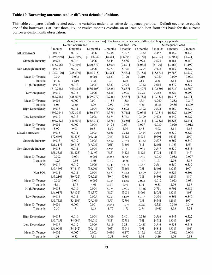
73
Table 10. Borrowing outcomes under different default definitions This table compares default-related outcome variables under alternative delinquency periods. Default occurrence equals one if the borrower is at least three, six, or twelve months overdue on at least one loan from this bank for the current borrower-bank-month observation.
Mean [number of observations] of outcome variables under different delinquency periods Default occurrence Resolution Time Subsequent Loans
3 months 6 months 12 months 3 months 6 months 12 months 3 months 6 months 12 months All Borrowers 0.018 0.012 0.006 7.738 8.727 10.152 0.487 0.459 0.433
[1,394,466] [1,297,999] [1,116,087] [18,751] [11,304] [4,185] [20,703] [13,052] [4,931] Strategic Industry 0.021 0.014 0.006 7.644 8.586 9.992 0.525 0.481 0.450
[335,296] [312,469] [270,872] [4,800] [2,871] [1,033] [5,120] [3,164] [1,192] Non-Strategic Industry 0.017 0.012 0.006 7.771 8.775 10.204 0.475 0.452 0.427
[1,059,170] [985,530] [845,215] [13,951] [8,433] [3,152] [15,583] [9,888] [3,739] Mean Difference -0.004 -0.002 -0.001 0.127 0.190 0.210 -0.050 -0.029 -0.023
T-statistic -14.23 -11.10 -3.86 1.01 1.03 0.62 -2.35 -3.64 -1.02 High Frequency 0.017 0.013 0.005 8.323 9.494 10.712 0.615 0.579 0.537
[710,228] [669,392] [586,108] [9,525] [5,837] [2,427] [10,550] [6,834] [2,860] Low Frequency 0.019 0.015 0.006 7.135 7.908 9.378 0.355 0.327 0.290
[684,238] [628,607] [529,979] [9,226] [5,467] [1,758] [10,153] [6,218] [2,071] Mean Difference 0.002 0.002 0.001 -1.188 -1.586 -1.334 -0.260 -0.252 -0.247
T-statistic 6.06 2.30 1.99 -9.97 -10.45 -4.35 -38.85 -29.86 -18.09 High Dependency 0.017 0.011 0.004 7.800 8.692 10.102 0.502 0.469 0.439
[697,234] [652,398] [550,176] [9,375] [5,718] [2,034] [10,351] [6,529] [2,490] Low Dependency 0.019 0.013 0.008 7.674 8.763 10.199 0.472 0.449 0.427
[697,232] [645,601] [565,911] [9,376] [5,586] [2,151] [10,352] [6,523] [2,441] Mean Difference 0.002 0.002 0.004 -0.126 0.071 0.097 -0.030 -0.020 -0.012
T-statistic 8.92 9.03 10.81 -1.57 1.09 1.45 -4.02 -3.11 -2.58 Listed Borrowers 0.016 0.011 0.005 7.665 7.312 10.414 0.556 0.539 0.520
[72,669] [68,338] [60,426] [946] [582] [193] [979] [612] [200] Strategic Industry 0.017 0.012 0.005 7.852 7.764 11.752 0.577 0.562 0.540
[21,317] [20,115] [17,933] [261] [160] [51] [276] [173] [53] Non-Strategic Industry 0.015 0.011 0.004 7.594 7.141 9.933 0.547 0.530 0.513
[51,352] [48,223] [42,493] [685] [422] [142] [703] [439] [147] Mean Difference -0.002 -0.001 -0.001 -0.258 -0.623 -1.819 -0.030 -0.032 -0.027
T-statistic -1.25 -0.98 -1.68 -0.42 -0.76 -1.07 -1.91 -2.06 -3.17 SOE 0.019 0.012 0.006 6.943 6.504 9.387 0.561 0.550 0.537
[39,459] [37,416] [33,705] [552] [326] [95] [540] [322] [90] Non SOE 0.014 0.011 0.004 8.677 8.342 11.409 0.549 0.527 0.506
[33,210] [30,922] [26,721] [394] [256] [98] [439] [290] [110] Mean Difference -0.005 -0.001 -0.002 1.734 1.838 2.022 -0.012 -0.023 -0.031
T-statistic -4.61 -1.77 -4.01 3.27 2.49 1.34 -0.38 -2.06 -1.37 High Frequency 0.015 0.010 0.004 8.074 7.923 12.336 0.711 0.701 0.689
[36,917] [35,132] [31,377] [487] [303] [100] [505] [321] [103] Low Frequency 0.016 0.011 0.005 7.231 6.649 8.347 0.390 0.361 0.340
[35,752] [33,206] [29,049] [459] [279] [93] [474] [291] [97] Mean Difference 0.001 0.000 0.001 -0.843 -1.274 -3.989 -0.321 -0.340 -0.349
T-statistic 2.30 1.71 1.63 -1.77 -1.75 -2.74 -10.65 -8.93 -5.24
High Dependency 0.015 0.010 0.004 7.709 7.401 10.336 0.566 0.545 0.522 [35,765] [34,096] [30,015] [481] [278] [94] [498] [301] [99]
Low Dependency 0.017 0.012 0.006 7.619 7.231 10.488 0.546 0.533 0.518 [36,904] [34,242] [30,411] [465] [304] [99] [481] [311] [101]
Mean Difference 0.002 0.002 0.002 -0.090 -0.170 0.152 -0.020 -0.012 -0.004 T-statistic 4.38 6.32 7.11 -0.53 -0.92 1.08 -3.19 -1.76 -0.83
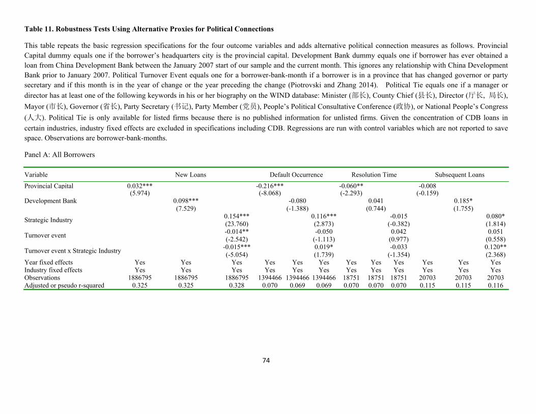
74
Table 11. Robustness Tests Using Alternative Proxies for Political Connections
This table repeats the basic regression specifications for the four outcome variables and adds alternative political connection measures as follows. Provincial Capital dummy equals one if the borrower’s headquarters city is the provincial capital. Development Bank dummy equals one if borrower has ever obtained a loan from China Development Bank between the January 2007 start of our sample and the current month. This ignores any relationship with China Development Bank prior to January 2007. Political Turnover Event equals one for a borrower-bank-month if a borrower is in a province that has changed governor or party secretary and if this month is in the year of change or the year preceding the change (Piotrovski and Zhang 2014). Political Tie equals one if a manager or
director has at least one of the following keywords in his or her biography on the WIND database: Minister (部长), County Chief (县长), Director (厅长, 局长),
Mayor (市长), Governor (省长), Party Secretary (书记), Party Member (党员), People’s Political Consultative Conference (政协), or National People’s Congress
(人大). Political Tie is only available for listed firms because there is no published information for unlisted firms. Given the concentration of CDB loans in
certain industries, industry fixed effects are excluded in specifications including CDB. Regressions are run with control variables which are not reported to save space. Observations are borrower-bank-months.
Panel A: All Borrowers
Variable New Loans Default Occurrence Resolution Time Subsequent Loans
Provincial Capital 0.032*** -0.216*** -0.060** -0.008 (5.974) (-8.068) (-2.293) (-0.159)Development Bank 0.098*** -0.080 0.041 0.185* (7.529) (-1.388) (0.744) (1.755)
Strategic Industry 0.154*** 0.116*** -0.015 0.080* (23.760) (2.873) (-0.382) (1.814)
Turnover event -0.014** -0.050 0.042 0.051 (-2.542) (-1.113) (0.977) (0.558)
Turnover event x Strategic Industry -0.015*** 0.019* -0.033 0.120** (-5.054) (1.739) (-1.354) (2.368)
Year fixed effects Yes Yes Yes Yes Yes Yes Yes Yes Yes Yes Yes Yes Industry fixed effects Yes Yes Yes Yes Yes Yes Yes Yes Yes Yes Yes Yes Observations 1886795 1886795 1886795 1394466 1394466 1394466 18751 18751 18751 20703 20703 20703 Adjusted or pseudo r-squared 0.325 0.325 0.328 0.070 0.069 0.069 0.070 0.070 0.070 0.115 0.115 0.116
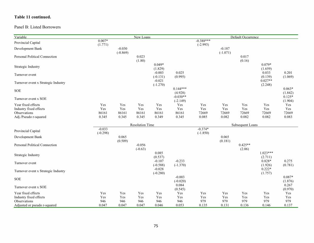
75
Table 11 continued.
Panel B: Listed Borrowers
Variable New Loans Default Occurrence
Provincial Capital 0.007* -0.388***(1.771) (-2.993)
Development Bank -0.030 -0.187(-0.869) (-1.071)
Personal Political Connection 0.023 0.017(1.80) (0.16)
Strategic Industry 0.049* 0.079*(1.829) (1.659)
Turnover event -0.003 0.025 0.033 0.201(-0.131) (0.995) (0.139) (1.069)
Turnover event x Strategic Industry -0.021 0.027**(-1.270) (2.248)
SOE 0.144*** 0.063*(4.928) (1.842)
Turnover event x SOE -0.030** 0.125*(-2.149) (1.904)
Year fixed effects Yes Yes Yes Yes Yes Yes Yes Yes Yes YesIndustry fixed effects Yes Yes Yes Yes Yes Yes Yes Yes Yes YesObservations 86161 86161 86161 86161 86161 72669 72669 72669 72669 72669Adj./Pseudo r-squared 0.345 0.345 0.345 0.349 0.345 0.085 0.082 0.082 0.082 0.083
Resolution Time Subsequent Loans
Provincial Capital -0.033 -0.374*(-0.298) (-1.850)
Development Bank 0.065 0.065(0.509) (0.181)
Personal Political Connection -0.056 0.425**(-0.63) (2.06)
Strategic Industry 0.085 1.023***(0.537) (2.711)
Turnover event -0.107 -0.233 0.828* 0.275(-0.588) (-1.370) (1.926) (0.781)
Turnover event x Strategic Industry -0.028 0.222*(-0.280) (1.757)
SOE -0.003 0.087*(-0.020) (1.876)
Turnover event x SOE 0.084 0.267(0.545) (0.970)
Year fixed effects Yes Yes Yes Yes Yes Yes Yes Yes Yes YesIndustry fixed effects Yes Yes Yes Yes Yes Yes Yes Yes Yes YesObservations 946 946 946 946 946 979 979 979 979 979Adjusted or pseudo r-squared 0.047 0.047 0.047 0.046 0.053 0.135 0.131 0.136 0.146 0.137

76
Table A1. Variable Definitions
Currency amounts are quoted in Chinese yuan, indicated by RMB. During the period we study, the exchange rate rose from about eight yuan per US dollar to about six per US dollar.
New Loans (Million RMB)
The total amount of newly extended loans to a firm by a bank in a month.
Default Occurrence A dummy variable equal to 1 if at least one loan extended by a particular bank to a firm in a month is in default and 0 otherwise. We define default as three months delinquent or going bankrupt.
Resolution Time The longest resolution time for defaulted loans of a given bank-borrower pair that matures in the given month.
Subsequent Loan Availability after Default
A dummy variable equal to 1 if a firm obtains a new loan from the same bank within 3 months after defaulting on a loan from this bank in the given month.
Assets (Billion RMB)
Total assets of the firm.
Leverage The ratio of liabilities to assets.
Nonperforming loans
The ratio of non-performing loans to all loans obtained by the firm from the bank cumulated to the current month.
Number of Lenders The total number of distinct banks that the firm has ever borrowed from measured from the start of the sample period to the current month. It varies across borrowers and months but not across borrower-banks holding month constant.
Group Assets (Billion RMB)
The total book value of assets of all group members. It is set to zero for firms that are not members of a group.
Group NPL The ratio of nonperforming loans to total loans for all group members except this firm from all banks as of the current month. It is set to zero for firms that are not members of a group.
Risk Signal The number of “risk” signals as assessed by loan managers. The five types of risks are: bad corporate governance, complex corporate structure and network of relationships with other firms, excessive product and geographic diversification, highly volatile cash flows, and high leverage.
Strategic Industry
A dummy variable equal to 1 if the borrower is associated with a so-called strategic industry (sectors of interest to the government such as mining, real estate, media and culture, power, gas, and water, transportation and storage, banking, finance and insurance, metals and non-metals, petrochemicals, and rubber). For listed borrowers, this is determined directly from the two-digit industry code which is available yearly. For unlisted borrowers, loans are tagged by industry and we tag the firm with the industry tag associated with the highest total amount of its loans within a given year.
Frequency The number of times that a firm has obtained loans from this bank from the start of the sample period to the current month.
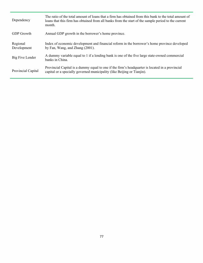
77
Dependency The ratio of the total amount of loans that a firm has obtained from this bank to the total amount of loans that this firm has obtained from all banks from the start of the sample period to the current month.
GDP Growth Annual GDP growth in the borrower’s home province.
Regional Development
Index of economic development and financial reform in the borrower’s home province developed by Fan, Wang, and Zhang (2001).
Big Five Lender A dummy variable equal to 1 if a lending bank is one of the five large state-owned commercial banks in China.
Provincial Capital Provincial Capital is a dummy equal to one if the firm’s headquarter is located in a provincial capital or a specially governed municipality (like Beijing or Tianjin).
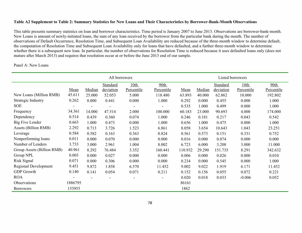
78
Table A2 Supplement to Table 2: Summary Statistics for New Loans and Their Characteristics by Borrower-Bank-Month Observations This table presents summary statistics on loan and borrower characteristics. Time period is January 2007 to June 2013. Observations are borrower-bank-month. New Loans is amount of newly-initiated loans, the sum of any loan received by the borrower from the particular bank during the month. The number of observations of Default Occurrence, Resolution Time, and Subsequent Loan Availability are reduced because of the three-month window to determine default, the computation of Resolution Time and Subsequent Loan Availability only for loans that have defaulted, and a further three-month window to determine whether there is a subsequent new loan. In particular, the number of observations for Resolution Time is reduced because it uses defaulted loans only (does not mature after March 2013) and requires that resolution occur at or before the June 2013 end of our sample. Panel A: New Loans
All borrowers Listed borrowers
Mean MedianStandard deviation
10th Percentile
90th Percentile Mean Median
Standard deviation
10th Percentile
90th Percentile
New Loans (Million RMB) 45.611 25.000 52.053 5.000 118.480 63.893 40.000 62.862 10.000 192.802 Strategic Industry 0.262 0.000 0.441 0.000 1.000 0.292 0.000 0.455 0.000 1.000 SOE - - - - - 0.535 1.000 0.499 0.000 1.000 Frequency 34.361 14.000 47.514 2.000 100.000 60.183 23.000 90.693 4.000 174.000 Dependency 0.514 0.439 0.360 0.074 1.000 0.246 0.181 0.217 0.043 0.542 Big Five Lender 0.663 1.000 0.473 0.000 1.000 0.656 1.000 0.475 0.000 1.000 Assets (Billion RMB) 2.292 0.713 3.726 1.523 6.861 8.058 3.654 10.643 1.043 23.251 Leverage 0.584 0.582 0.163 0.363 0.824 0.561 0.573 0.151 0.331 0.752 Nonperforming loans 0.011 0.000 0.070 0.000 0.000 0.016 0.000 0.074 0.000 0.000 Number of Lenders 3.733 3.000 2.961 1.004 8.002 6.723 6.000 3.208 3.000 11.000 Group Assets (Billion RMB) 40.961 8.292 76.484 3.352 160.441 110.932 29.290 151.735 8.291 342.632 Group NPL 0.003 0.000 0.027 0.000 0.000 0.006 0.000 0.026 0.000 0.010 Risk Signal 0.071 0.000 0.306 0.000 0.000 0.234 0.000 0.545 0.000 1.000 Regional Development 9.451 9.872 1.858 6.570 11.452 9.002 9.022 1.919 6.171 11.452 GDP Growth 0.140 0.141 0.054 0.071 0.211 0.152 0.156 0.055 0.072 0.221 ROA - - - - - 0.020 0.018 0.033 -0.006 0.052 Observations 1886795 86161 Borrowers 153955 1862
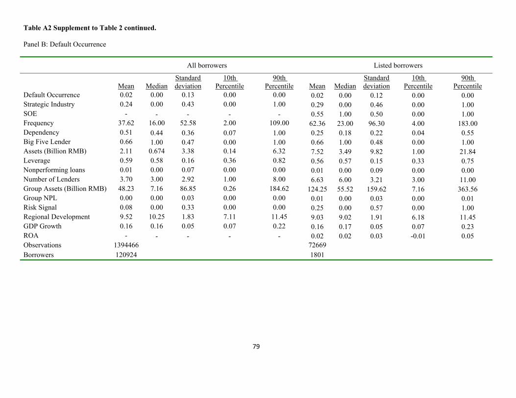
79
Table A2 Supplement to Table 2 continued. Panel B: Default Occurrence
All borrowers Listed borrowers
Mean MedianStandard deviation
10th Percentile
90th Percentile Mean Median
Standard deviation
10th Percentile
90th Percentile
Default Occurrence 0.02 0.00 0.13 0.00 0.00 0.02 0.00 0.12 0.00 0.00 Strategic Industry 0.24 0.00 0.43 0.00 1.00 0.29 0.00 0.46 0.00 1.00 SOE - - - - - 0.55 1.00 0.50 0.00 1.00 Frequency 37.62 16.00 52.58 2.00 109.00 62.36 23.00 96.30 4.00 183.00 Dependency 0.51 0.44 0.36 0.07 1.00 0.25 0.18 0.22 0.04 0.55 Big Five Lender 0.66 1.00 0.47 0.00 1.00 0.66 1.00 0.48 0.00 1.00 Assets (Billion RMB) 2.11 0.674 3.38 0.14 6.32 7.52 3.49 9.82 1.00 21.84 Leverage 0.59 0.58 0.16 0.36 0.82 0.56 0.57 0.15 0.33 0.75 Nonperforming loans 0.01 0.00 0.07 0.00 0.00 0.01 0.00 0.09 0.00 0.00 Number of Lenders 3.70 3.00 2.92 1.00 8.00 6.63 6.00 3.21 3.00 11.00 Group Assets (Billion RMB) 48.23 7.16 86.85 0.26 184.62 124.25 55.52 159.62 7.16 363.56 Group NPL 0.00 0.00 0.03 0.00 0.00 0.01 0.00 0.03 0.00 0.01 Risk Signal 0.08 0.00 0.33 0.00 0.00 0.25 0.00 0.57 0.00 1.00 Regional Development 9.52 10.25 1.83 7.11 11.45 9.03 9.02 1.91 6.18 11.45 GDP Growth 0.16 0.16 0.05 0.07 0.22 0.16 0.17 0.05 0.07 0.23 ROA - - - - - 0.02 0.02 0.03 -0.01 0.05 Observations 1394466 72669 Borrowers 120924 1801
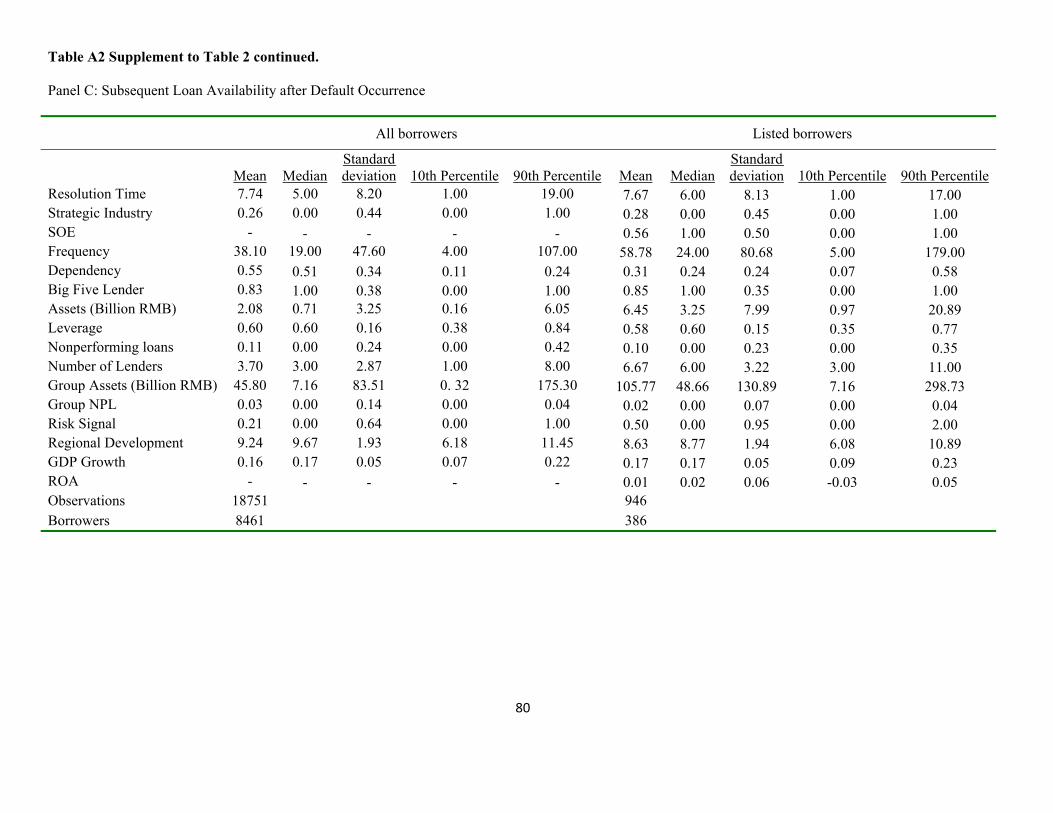
80
Table A2 Supplement to Table 2 continued. Panel C: Subsequent Loan Availability after Default Occurrence
All borrowers Listed borrowers
Mean MedianStandard deviation 10th Percentile 90th Percentile Mean Median
Standard deviation 10th Percentile 90th Percentile
Resolution Time 7.74 5.00 8.20 1.00 19.00 7.67 6.00 8.13 1.00 17.00 Strategic Industry 0.26 0.00 0.44 0.00 1.00 0.28 0.00 0.45 0.00 1.00 SOE - - - - - 0.56 1.00 0.50 0.00 1.00 Frequency 38.10 19.00 47.60 4.00 107.00 58.78 24.00 80.68 5.00 179.00 Dependency 0.55 0.51 0.34 0.11 0.24 0.31 0.24 0.24 0.07 0.58 Big Five Lender 0.83 1.00 0.38 0.00 1.00 0.85 1.00 0.35 0.00 1.00 Assets (Billion RMB) 2.08 0.71 3.25 0.16 6.05 6.45 3.25 7.99 0.97 20.89 Leverage 0.60 0.60 0.16 0.38 0.84 0.58 0.60 0.15 0.35 0.77 Nonperforming loans 0.11 0.00 0.24 0.00 0.42 0.10 0.00 0.23 0.00 0.35 Number of Lenders 3.70 3.00 2.87 1.00 8.00 6.67 6.00 3.22 3.00 11.00 Group Assets (Billion RMB) 45.80 7.16 83.51 0. 32 175.30 105.77 48.66 130.89 7.16 298.73 Group NPL 0.03 0.00 0.14 0.00 0.04 0.02 0.00 0.07 0.00 0.04 Risk Signal 0.21 0.00 0.64 0.00 1.00 0.50 0.00 0.95 0.00 2.00 Regional Development 9.24 9.67 1.93 6.18 11.45 8.63 8.77 1.94 6.08 10.89 GDP Growth 0.16 0.17 0.05 0.07 0.22 0.17 0.17 0.05 0.09 0.23 ROA - - - - - 0.01 0.02 0.06 -0.03 0.05 Observations 18751 946 Borrowers 8461 386
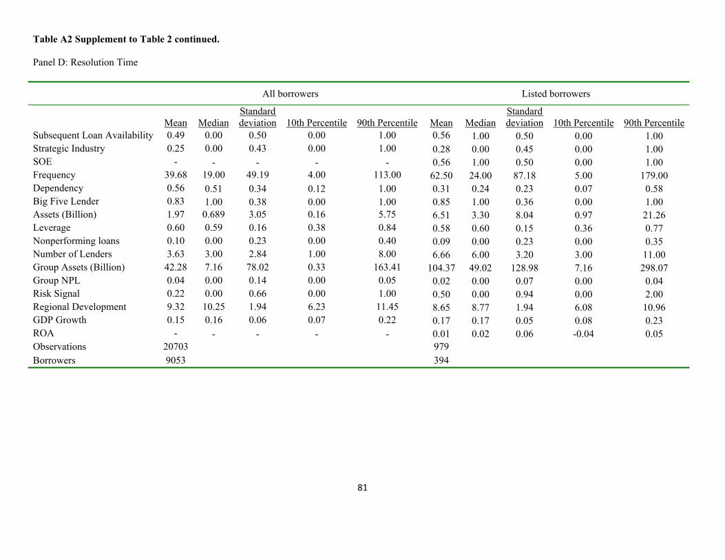
81
Table A2 Supplement to Table 2 continued. Panel D: Resolution Time
All borrowers Listed borrowers
Mean MedianStandard deviation 10th Percentile 90th Percentile Mean Median
Standard deviation 10th Percentile 90th Percentile
Subsequent Loan Availability 0.49 0.00 0.50 0.00 1.00 0.56 1.00 0.50 0.00 1.00 Strategic Industry 0.25 0.00 0.43 0.00 1.00 0.28 0.00 0.45 0.00 1.00 SOE - - - - - 0.56 1.00 0.50 0.00 1.00 Frequency 39.68 19.00 49.19 4.00 113.00 62.50 24.00 87.18 5.00 179.00 Dependency 0.56 0.51 0.34 0.12 1.00 0.31 0.24 0.23 0.07 0.58 Big Five Lender 0.83 1.00 0.38 0.00 1.00 0.85 1.00 0.36 0.00 1.00 Assets (Billion) 1.97 0.689 3.05 0.16 5.75 6.51 3.30 8.04 0.97 21.26 Leverage 0.60 0.59 0.16 0.38 0.84 0.58 0.60 0.15 0.36 0.77 Nonperforming loans 0.10 0.00 0.23 0.00 0.40 0.09 0.00 0.23 0.00 0.35 Number of Lenders 3.63 3.00 2.84 1.00 8.00 6.66 6.00 3.20 3.00 11.00 Group Assets (Billion) 42.28 7.16 78.02 0.33 163.41 104.37 49.02 128.98 7.16 298.07 Group NPL 0.04 0.00 0.14 0.00 0.05 0.02 0.00 0.07 0.00 0.04 Risk Signal 0.22 0.00 0.66 0.00 1.00 0.50 0.00 0.94 0.00 2.00 Regional Development 9.32 10.25 1.94 6.23 11.45 8.65 8.77 1.94 6.08 10.96 GDP Growth 0.15 0.16 0.06 0.07 0.22 0.17 0.17 0.05 0.08 0.23 ROA - - - - - 0.01 0.02 0.06 -0.04 0.05 Observations 20703 979 Borrowers 9053 394
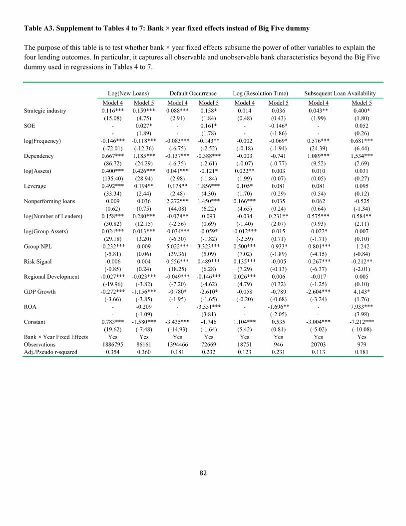
82
Table A3. Supplement to Tables 4 to 7: Bank × year fixed effects instead of Big Five dummy
The purpose of this table is to test whether bank × year fixed effects subsume the power of other variables to explain the four lending outcomes. In particular, it captures all observable and unobservable bank characteristics beyond the Big Five dummy used in regressions in Tables 4 to 7.
Log(New Loans) Default Occurrence Log (Resolution Time) Subsequent Loan Availability
Model 4 Model 5 Model 4 Model 5 Model 4 Model 5 Model 4 Model 5 Strategic industry 0.116*** 0.159*** 0.088*** 0.158* 0.014 0.036 0.043** 0.400* (15.08) (4.75) (2.91) (1.84) (0.48) (0.43) (1.99) (1.80) SOE - 0.027* - 0.161* - -0.146* - 0.052 - (1.89) - (1.78) - (-1.86) - (0.26) log(Frequency) -0.146*** -0.118*** -0.083*** -0.143** -0.002 -0.069* 0.576*** 0.681*** (-72.01) (-12.36) (-6.75) (-2.52) (-0.18) (-1.94) (24.39) (6.44) Dependency 0.667*** 1.185*** -0.137*** -0.388*** -0.003 -0.741 1.089*** 1.534*** (86.72) (24.29) (-6.35) (-2.61) (-0.07) (-0.77) (9.52) (2.69) log(Assets) 0.400*** 0.426*** 0.041*** -0.121* 0.022** 0.003 0.010 0.031 (135.40) (28.94) (2.98) (-1.84) (1.99) (0.07) (0.05) (0.27) Leverage 0.492*** 0.194** 0.178** 1.856*** 0.105* 0.081 0.081 0.095 (33.34) (2.44) (2.48) (4.30) (1.70) (0.29) (0.54) (0.12) Nonperforming loans 0.009 0.036 2.272*** 1.450*** 0.166*** 0.035 0.062 -0.525 (0.62) (0.75) (44.08) (6.22) (4.65) (0.24) (0.64) (-1.34) log(Number of Lenders) 0.158*** 0.280*** -0.078** 0.093 -0.034 0.231** 0.575*** 0.584** (30.82) (12.15) (-2.56) (0.69) (-1.40) (2.07) (9.93) (2.11) log(Group Assets) 0.024*** 0.013*** -0.034*** -0.059* -0.012*** 0.015 -0.022* 0.007 (29.18) (3.20) (-6.30) (-1.82) (-2.59) (0.71) (-1.71) (0.10) Group NPL -0.232*** 0.009 5.022*** 3.323*** 0.500*** -0.933* -0.801*** -1.242 (-5.81) (0.06) (39.36) (5.09) (7.02) (-1.89) (-4.15) (-0.84) Risk Signal -0.006 0.004 0.556*** 0.489*** 0.135*** -0.005 -0.267*** -0.212** (-0.85) (0.24) (18.25) (6.28) (7.29) (-0.13) (-6.37) (-2.01) Regional Development -0.027*** -0.023*** -0.049*** -0.146*** 0.026*** 0.006 -0.017 0.005 (-19.96) (-3.82) (-7.20) (-4.62) (4.79) (0.32) (-1.25) (0.10) GDP Growth -0.272*** -1.156*** -0.780* -2.610* -0.058 -0.789 -2.604*** 4.143* (-3.66) (-3.85) (-1.95) (-1.65) (-0.20) (-0.68) (-3.24) (1.76) ROA - -0.209 - -3.331*** - -1.696** - 7.933*** - (-1.09) - (3.81) - (-2.05) - (3.98) Constant 0.783*** -1.580*** -3.435*** -1.746 1.104*** 0.535 -3.004*** -7.212*** (19.62) (-7.48) (-14.93) (-1.64) (5.42) (0.81) (-5.02) (-10.08) Bank × Year Fixed Effects Yes Yes Yes Yes Yes Yes Yes Yes Observations 1886795 86161 1394466 72669 18751 946 20703 979 Adj./Pseudo r-squared 0.354 0.360 0.181 0.232 0.123 0.231 0.113 0.181
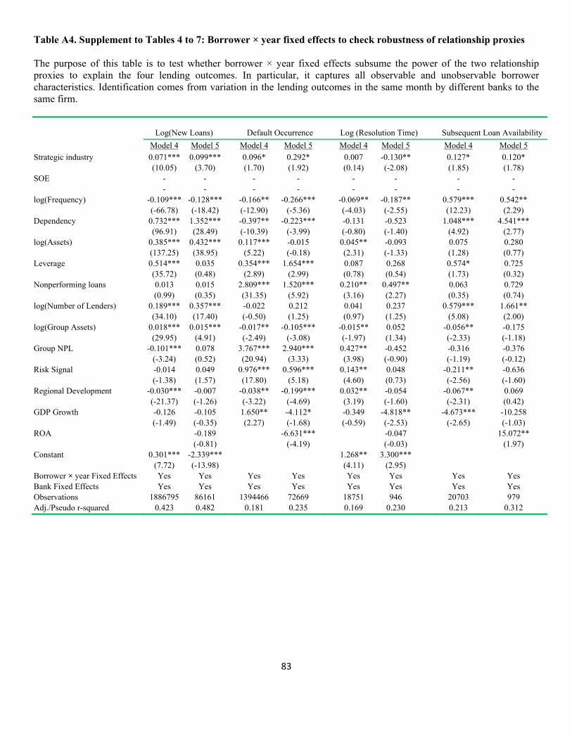
83
Table A4. Supplement to Tables 4 to 7: Borrower × year fixed effects to check robustness of relationship proxies The purpose of this table is to test whether borrower × year fixed effects subsume the power of the two relationship proxies to explain the four lending outcomes. In particular, it captures all observable and unobservable borrower characteristics. Identification comes from variation in the lending outcomes in the same month by different banks to the same firm.
Log(New Loans) Default Occurrence Log (Resolution Time) Subsequent Loan Availability
Model 4 Model 5 Model 4 Model 5 Model 4 Model 5 Model 4 Model 5
Strategic industry 0.071*** 0.099*** 0.096* 0.292* 0.007 -0.130** 0.127* 0.120* (10.05) (3.70) (1.70) (1.92) (0.14) (-2.08) (1.85) (1.78) SOE - - - - - - - - - - - - - - - - log(Frequency) -0.109*** -0.128*** -0.166** -0.266*** -0.069** -0.187** 0.579*** 0.542** (-66.78) (-18.42) (-12.90) (-5.36) (-4.03) (-2.55) (12.23) (2.29) Dependency 0.732*** 1.352*** -0.397** -0.223*** -0.131 -0.523 1.048*** 4.541*** (96.91) (28.49) (-10.39) (-3.99) (-0.80) (-1.40) (4.92) (2.77) log(Assets) 0.385*** 0.432*** 0.117*** -0.015 0.045** -0.093 0.075 0.280 (137.25) (38.95) (5.22) (-0.18) (2.31) (-1.33) (1.28) (0.77) Leverage 0.514*** 0.035 0.354*** 1.654*** 0.087 0.268 0.574* 0.725 (35.72) (0.48) (2.89) (2.99) (0.78) (0.54) (1.73) (0.32) Nonperforming loans 0.013 0.015 2.809*** 1.520*** 0.210** 0.497** 0.063 0.729 (0.99) (0.35) (31.35) (5.92) (3.16) (2.27) (0.35) (0.74) log(Number of Lenders) 0.189*** 0.357*** -0.022 0.212 0.041 0.237 0.579*** 1.661** (34.10) (17.40) (-0.50) (1.25) (0.97) (1.25) (5.08) (2.00) log(Group Assets) 0.018*** 0.015*** -0.017** -0.105*** -0.015** 0.052 -0.056** -0.175 (29.95) (4.91) (-2.49) (-3.08) (-1.97) (1.34) (-2.33) (-1.18) Group NPL -0.101*** 0.078 3.767*** 2.940*** 0.427** -0.452 -0.316 -0.376 (-3.24) (0.52) (20.94) (3.33) (3.98) (-0.90) (-1.19) (-0.12) Risk Signal -0.014 0.049 0.976*** 0.596*** 0.143** 0.048 -0.211** -0.636 (-1.38) (1.57) (17.80) (5.18) (4.60) (0.73) (-2.56) (-1.60) Regional Development -0.030*** -0.007 -0.038** -0.199*** 0.032** -0.054 -0.067** 0.069 (-21.37) (-1.26) (-3.22) (-4.69) (3.19) (-1.60) (-2.31) (0.42) GDP Growth -0.126 -0.105 1.650** -4.112* -0.349 -4.818** -4.673*** -10.258 (-1.49) (-0.35) (2.27) (-1.68) (-0.59) (-2.53) (-2.65) (-1.03) ROA -0.189 -6.631*** -0.047 15.072** (-0.81) (-4.19) (-0.03) (1.97) Constant 0.301*** -2.339*** 1.268** 3.300*** (7.72) (-13.98) (4.11) (2.95) Borrower × year Fixed Effects Yes Yes Yes Yes Yes Yes Yes Yes Bank Fixed Effects Yes Yes Yes Yes Yes Yes Yes Yes Observations 1886795 86161 1394466 72669 18751 946 20703 979 Adj./Pseudo r-squared 0.423 0.482 0.181 0.235 0.169 0.230 0.213 0.312
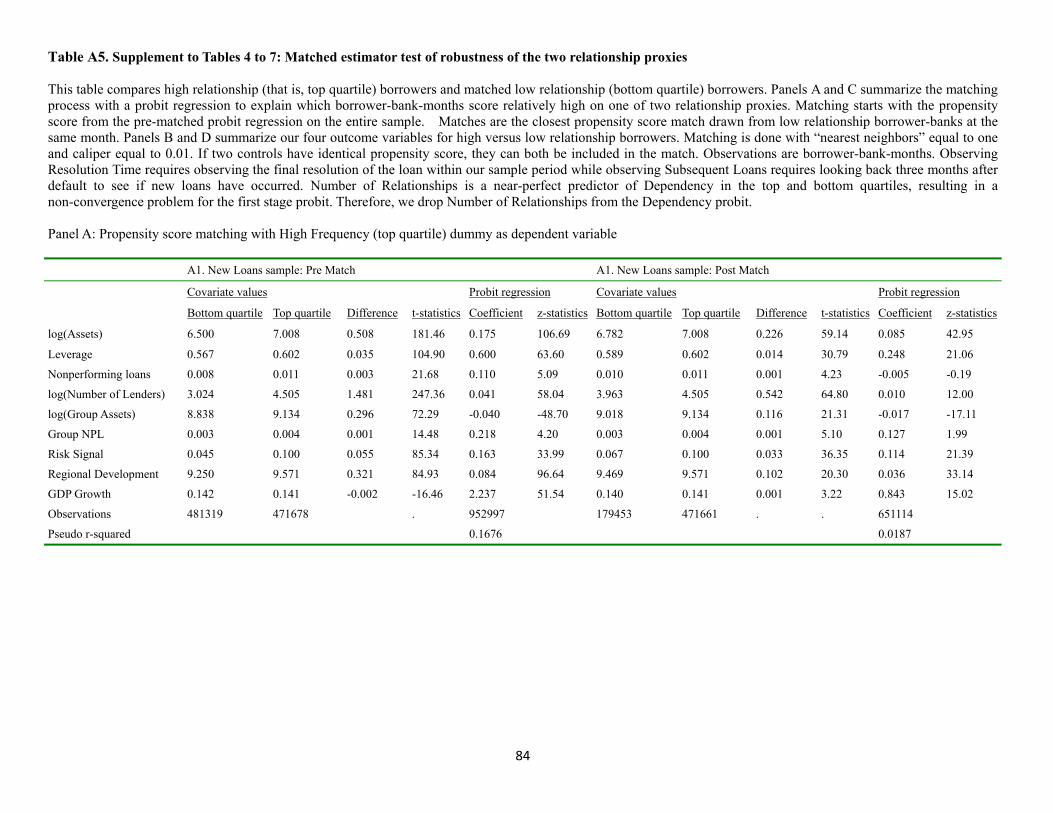
84
Table A5. Supplement to Tables 4 to 7: Matched estimator test of robustness of the two relationship proxies This table compares high relationship (that is, top quartile) borrowers and matched low relationship (bottom quartile) borrowers. Panels A and C summarize the matching process with a probit regression to explain which borrower-bank-months score relatively high on one of two relationship proxies. Matching starts with the propensity score from the pre-matched probit regression on the entire sample. Matches are the closest propensity score match drawn from low relationship borrower-banks at the same month. Panels B and D summarize our four outcome variables for high versus low relationship borrowers. Matching is done with “nearest neighbors” equal to one and caliper equal to 0.01. If two controls have identical propensity score, they can both be included in the match. Observations are borrower-bank-months. Observing Resolution Time requires observing the final resolution of the loan within our sample period while observing Subsequent Loans requires looking back three months after default to see if new loans have occurred. Number of Relationships is a near-perfect predictor of Dependency in the top and bottom quartiles, resulting in a non-convergence problem for the first stage probit. Therefore, we drop Number of Relationships from the Dependency probit. Panel A: Propensity score matching with High Frequency (top quartile) dummy as dependent variable
A1. New Loans sample: Pre Match A1. New Loans sample: Post Match
Covariate values Probit regression Covariate values Probit regression
Bottom quartile Top quartile Difference t-statistics Coefficient z-statistics Bottom quartile Top quartile Difference t-statistics Coefficient z-statistics
log(Assets) 6.500 7.008 0.508 181.46 0.175 106.69 6.782 7.008 0.226 59.14 0.085 42.95
Leverage 0.567 0.602 0.035 104.90 0.600 63.60 0.589 0.602 0.014 30.79 0.248 21.06
Nonperforming loans 0.008 0.011 0.003 21.68 0.110 5.09 0.010 0.011 0.001 4.23 -0.005 -0.19
log(Number of Lenders) 3.024 4.505 1.481 247.36 0.041 58.04 3.963 4.505 0.542 64.80 0.010 12.00
log(Group Assets) 8.838 9.134 0.296 72.29 -0.040 -48.70 9.018 9.134 0.116 21.31 -0.017 -17.11
Group NPL 0.003 0.004 0.001 14.48 0.218 4.20 0.003 0.004 0.001 5.10 0.127 1.99
Risk Signal 0.045 0.100 0.055 85.34 0.163 33.99 0.067 0.100 0.033 36.35 0.114 21.39
Regional Development 9.250 9.571 0.321 84.93 0.084 96.64 9.469 9.571 0.102 20.30 0.036 33.14
GDP Growth 0.142 0.141 -0.002 -16.46 2.237 51.54 0.140 0.141 0.001 3.22 0.843 15.02
Observations 481319 471678 . 952997 179453 471661 . . 651114
Pseudo r-squared 0.1676 0.0187
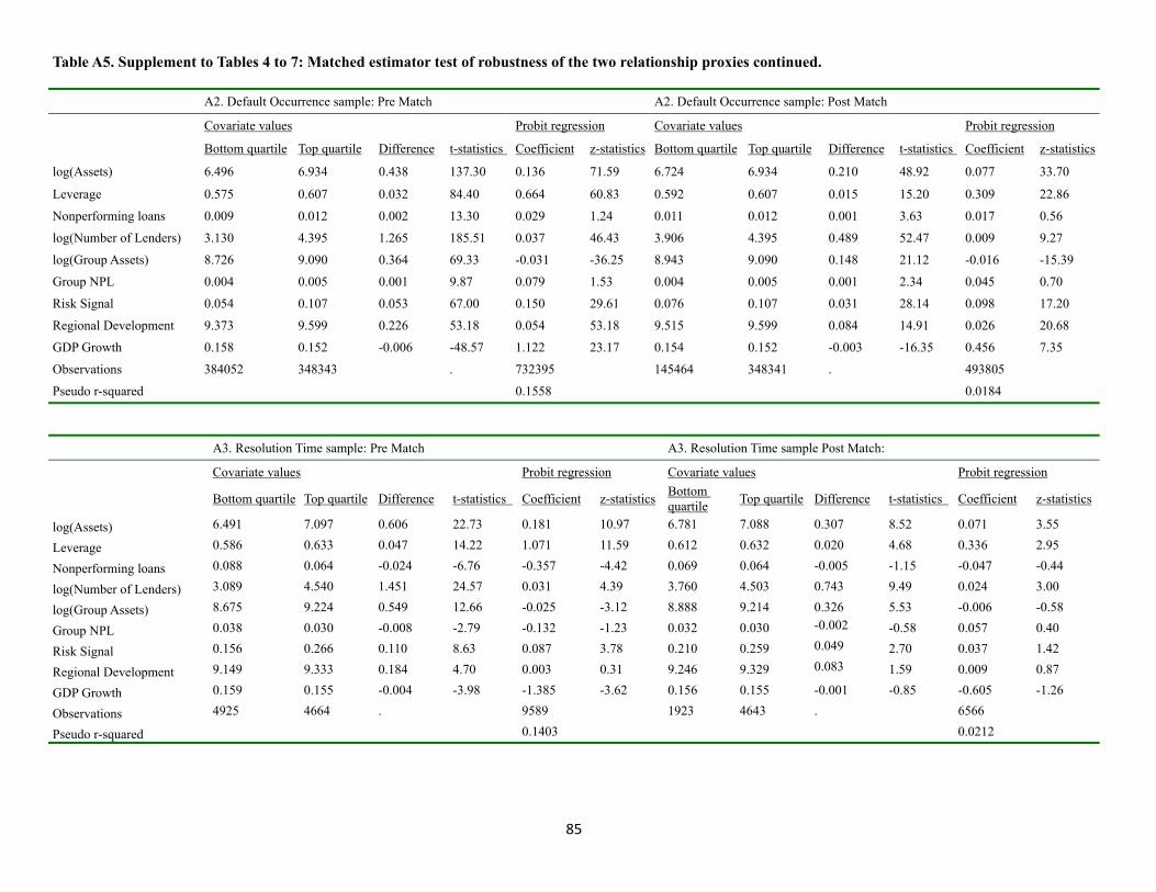
85
Table A5. Supplement to Tables 4 to 7: Matched estimator test of robustness of the two relationship proxies continued.
A2. Default Occurrence sample: Pre Match A2. Default Occurrence sample: Post Match
Covariate values Probit regression Covariate values Probit regression
Bottom quartile Top quartile Difference t-statistics Coefficient z-statistics Bottom quartile Top quartile Difference t-statistics Coefficient z-statistics
log(Assets) 6.496 6.934 0.438 137.30 0.136 71.59 6.724 6.934 0.210 48.92 0.077 33.70
Leverage 0.575 0.607 0.032 84.40 0.664 60.83 0.592 0.607 0.015 15.20 0.309 22.86
Nonperforming loans 0.009 0.012 0.002 13.30 0.029 1.24 0.011 0.012 0.001 3.63 0.017 0.56
log(Number of Lenders) 3.130 4.395 1.265 185.51 0.037 46.43 3.906 4.395 0.489 52.47 0.009 9.27
log(Group Assets) 8.726 9.090 0.364 69.33 -0.031 -36.25 8.943 9.090 0.148 21.12 -0.016 -15.39
Group NPL 0.004 0.005 0.001 9.87 0.079 1.53 0.004 0.005 0.001 2.34 0.045 0.70
Risk Signal 0.054 0.107 0.053 67.00 0.150 29.61 0.076 0.107 0.031 28.14 0.098 17.20
Regional Development 9.373 9.599 0.226 53.18 0.054 53.18 9.515 9.599 0.084 14.91 0.026 20.68
GDP Growth 0.158 0.152 -0.006 -48.57 1.122 23.17 0.154 0.152 -0.003 -16.35 0.456 7.35
Observations 384052 348343 . 732395 145464 348341 . 493805
Pseudo r-squared 0.1558 0.0184
A3. Resolution Time sample: Pre Match A3. Resolution Time sample Post Match:
Covariate values Probit regression Covariate values Probit regression
Bottom quartile Top quartile Difference t-statistics Coefficient z-statistics Bottom quartile
Top quartile Difference t-statistics Coefficient z-statistics
log(Assets) 6.491 7.097 0.606 22.73 0.181 10.97 6.781 7.088 0.307 8.52 0.071 3.55
Leverage 0.586 0.633 0.047 14.22 1.071 11.59 0.612 0.632 0.020 4.68 0.336 2.95
Nonperforming loans 0.088 0.064 -0.024 -6.76 -0.357 -4.42 0.069 0.064 -0.005 -1.15 -0.047 -0.44
log(Number of Lenders) 3.089 4.540 1.451 24.57 0.031 4.39 3.760 4.503 0.743 9.49 0.024 3.00
log(Group Assets) 8.675 9.224 0.549 12.66 -0.025 -3.12 8.888 9.214 0.326 5.53 -0.006 -0.58
Group NPL 0.038 0.030 -0.008 -2.79 -0.132 -1.23 0.032 0.030 -0.002 -0.58 0.057 0.40
Risk Signal 0.156 0.266 0.110 8.63 0.087 3.78 0.210 0.259 0.049 2.70 0.037 1.42
Regional Development 9.149 9.333 0.184 4.70 0.003 0.31 9.246 9.329 0.083 1.59 0.009 0.87
GDP Growth 0.159 0.155 -0.004 -3.98 -1.385 -3.62 0.156 0.155 -0.001 -0.85 -0.605 -1.26
Observations 4925 4664 . 9589 1923 4643 . 6566
Pseudo r-squared 0.1403 0.0212
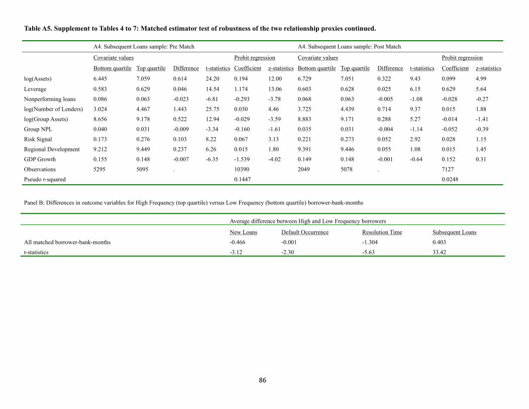
86
Table A5. Supplement to Tables 4 to 7: Matched estimator test of robustness of the two relationship proxies continued.
A4. Subsequent Loans sample: Pre Match A4. Subsequent Loans sample: Post Match
Covariate values Probit regression Covariate values Probit regression
Bottom quartile Top quartile Difference t-statistics Coefficient z-statistics Bottom quartile Top quartile Difference t-statistics Coefficient z-statistics
log(Assets) 6.445 7.059 0.614 24.20 0.194 12.00 6.729 7.051 0.322 9.43 0.099 4.99
Leverage 0.583 0.629 0.046 14.54 1.174 13.06 0.603 0.628 0.025 6.15 0.629 5.64
Nonperforming loans 0.086 0.063 -0.023 -6.81 -0.293 -3.78 0.068 0.063 -0.005 -1.08 -0.028 -0.27
log(Number of Lenders) 3.024 4.467 1.443 25.75 0.030 4.46 3.725 4.439 0.714 9.37 0.015 1.88
log(Group Assets) 8.656 9.178 0.522 12.94 -0.029 -3.59 8.883 9.171 0.288 5.27 -0.014 -1.41
Group NPL 0.040 0.031 -0.009 -3.34 -0.160 -1.61 0.035 0.031 -0.004 -1.14 -0.052 -0.39
Risk Signal 0.173 0.276 0.103 8.22 0.067 3.13 0.221 0.273 0.052 2.92 0.028 1.15
Regional Development 9.212 9.449 0.237 6.26 0.015 1.80 9.391 9.446 0.055 1.08 0.015 1.45
GDP Growth 0.155 0.148 -0.007 -6.35 -1.539 -4.02 0.149 0.148 -0.001 -0.64 0.152 0.31
Observations 5295 5095 . 10390 2049 5078 . 7127
Pseudo r-squared 0.1447 0.0248
Panel B: Differences in outcome variables for High Frequency (top quartile) versus Low Frequency (bottom quartile) borrower-bank-months
Average difference between High and Low Frequency borrowers
New Loans Default Occurrence Resolution Time Subsequent Loans
All matched borrower-bank-months -0.466 -0.001 -1.304 0.403
t-statistics -3.12 -2.30 -5.63 33.42
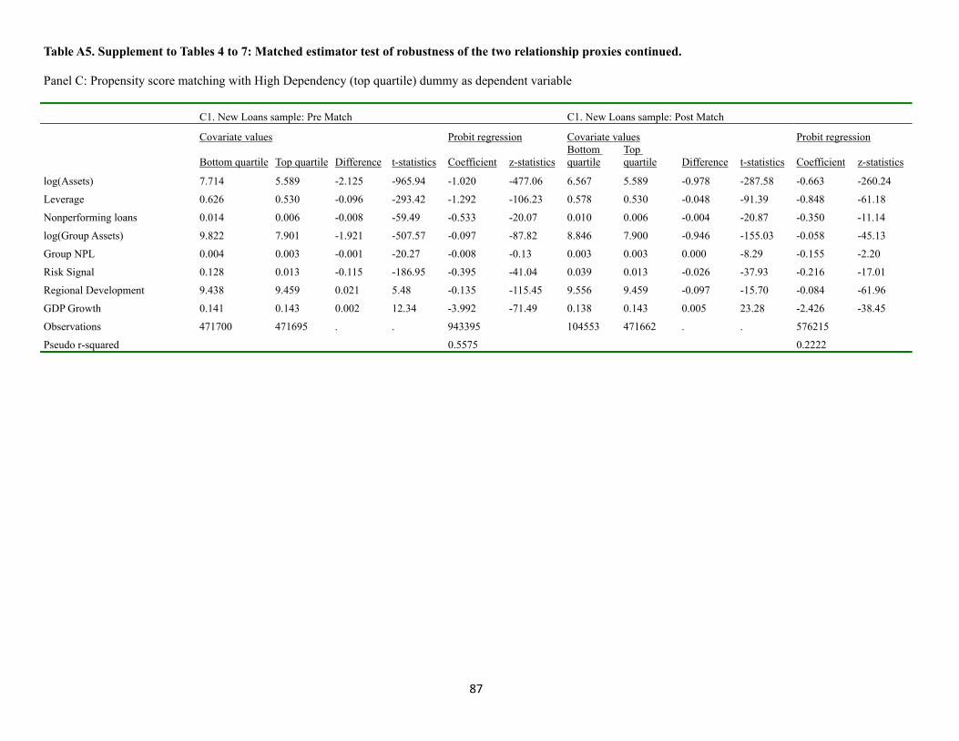
87
Table A5. Supplement to Tables 4 to 7: Matched estimator test of robustness of the two relationship proxies continued. Panel C: Propensity score matching with High Dependency (top quartile) dummy as dependent variable
C1. New Loans sample: Pre Match C1. New Loans sample: Post Match
Covariate values Probit regression Covariate values Probit regression
Bottom quartile Top quartile Difference t-statistics Coefficient z-statistics Bottom quartile
Top quartile Difference t-statistics Coefficient z-statistics
log(Assets) 7.714 5.589 -2.125 -965.94 -1.020 -477.06 6.567 5.589 -0.978 -287.58 -0.663 -260.24
Leverage 0.626 0.530 -0.096 -293.42 -1.292 -106.23 0.578 0.530 -0.048 -91.39 -0.848 -61.18
Nonperforming loans 0.014 0.006 -0.008 -59.49 -0.533 -20.07 0.010 0.006 -0.004 -20.87 -0.350 -11.14
log(Group Assets) 9.822 7.901 -1.921 -507.57 -0.097 -87.82 8.846 7.900 -0.946 -155.03 -0.058 -45.13
Group NPL 0.004 0.003 -0.001 -20.27 -0.008 -0.13 0.003 0.003 0.000 -8.29 -0.155 -2.20
Risk Signal 0.128 0.013 -0.115 -186.95 -0.395 -41.04 0.039 0.013 -0.026 -37.93 -0.216 -17.01
Regional Development 9.438 9.459 0.021 5.48 -0.135 -115.45 9.556 9.459 -0.097 -15.70 -0.084 -61.96
GDP Growth 0.141 0.143 0.002 12.34 -3.992 -71.49 0.138 0.143 0.005 23.28 -2.426 -38.45
Observations 471700 471695 . . 943395 104553 471662 . . 576215
Pseudo r-squared 0.5575 0.2222
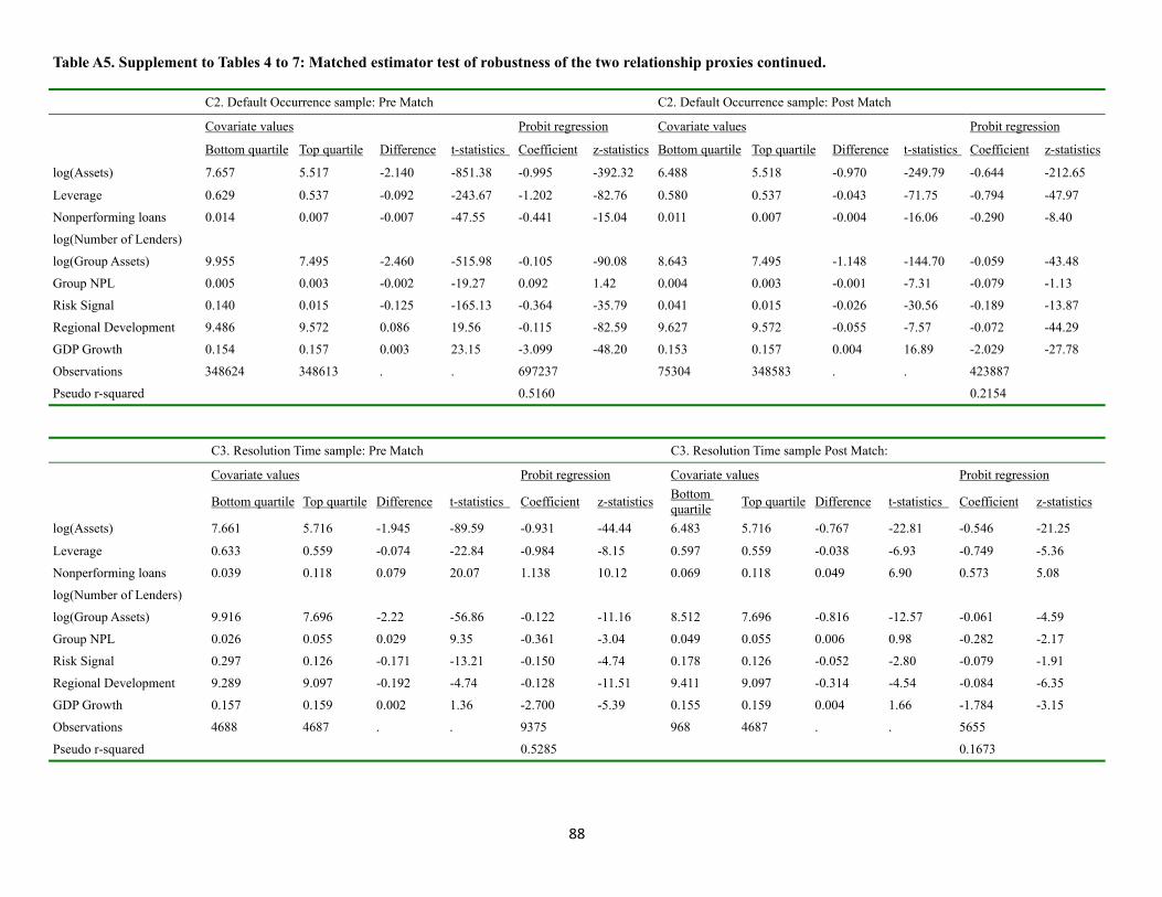
88
Table A5. Supplement to Tables 4 to 7: Matched estimator test of robustness of the two relationship proxies continued.
C2. Default Occurrence sample: Pre Match C2. Default Occurrence sample: Post Match
Covariate values Probit regression Covariate values Probit regression
Bottom quartile Top quartile Difference t-statistics Coefficient z-statistics Bottom quartile Top quartile Difference t-statistics Coefficient z-statistics
log(Assets) 7.657 5.517 -2.140 -851.38 -0.995 -392.32 6.488 5.518 -0.970 -249.79 -0.644 -212.65
Leverage 0.629 0.537 -0.092 -243.67 -1.202 -82.76 0.580 0.537 -0.043 -71.75 -0.794 -47.97
Nonperforming loans 0.014 0.007 -0.007 -47.55 -0.441 -15.04 0.011 0.007 -0.004 -16.06 -0.290 -8.40
log(Number of Lenders)
log(Group Assets) 9.955 7.495 -2.460 -515.98 -0.105 -90.08 8.643 7.495 -1.148 -144.70 -0.059 -43.48
Group NPL 0.005 0.003 -0.002 -19.27 0.092 1.42 0.004 0.003 -0.001 -7.31 -0.079 -1.13
Risk Signal 0.140 0.015 -0.125 -165.13 -0.364 -35.79 0.041 0.015 -0.026 -30.56 -0.189 -13.87
Regional Development 9.486 9.572 0.086 19.56 -0.115 -82.59 9.627 9.572 -0.055 -7.57 -0.072 -44.29
GDP Growth 0.154 0.157 0.003 23.15 -3.099 -48.20 0.153 0.157 0.004 16.89 -2.029 -27.78
Observations 348624 348613 . . 697237 75304 348583 . . 423887
Pseudo r-squared 0.5160 0.2154
C3. Resolution Time sample: Pre Match C3. Resolution Time sample Post Match:
Covariate values Probit regression Covariate values Probit regression
Bottom quartile Top quartile Difference t-statistics Coefficient z-statistics Bottomquartile
Top quartile Difference t-statistics Coefficient z-statistics
log(Assets) 7.661 5.716 -1.945 -89.59 -0.931 -44.44 6.483 5.716 -0.767 -22.81 -0.546 -21.25
Leverage 0.633 0.559 -0.074 -22.84 -0.984 -8.15 0.597 0.559 -0.038 -6.93 -0.749 -5.36
Nonperforming loans 0.039 0.118 0.079 20.07 1.138 10.12 0.069 0.118 0.049 6.90 0.573 5.08
log(Number of Lenders)
log(Group Assets) 9.916 7.696 -2.22 -56.86 -0.122 -11.16 8.512 7.696 -0.816 -12.57 -0.061 -4.59
Group NPL 0.026 0.055 0.029 9.35 -0.361 -3.04 0.049 0.055 0.006 0.98 -0.282 -2.17
Risk Signal 0.297 0.126 -0.171 -13.21 -0.150 -4.74 0.178 0.126 -0.052 -2.80 -0.079 -1.91
Regional Development 9.289 9.097 -0.192 -4.74 -0.128 -11.51 9.411 9.097 -0.314 -4.54 -0.084 -6.35
GDP Growth 0.157 0.159 0.002 1.36 -2.700 -5.39 0.155 0.159 0.004 1.66 -1.784 -3.15
Observations 4688 4687 . . 9375 968 4687 . . 5655
Pseudo r-squared 0.5285 0.1673
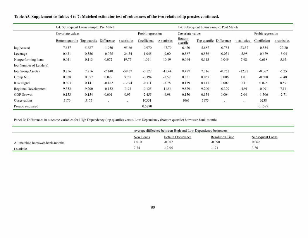
89
Table A5. Supplement to Tables 4 to 7: Matched estimator test of robustness of the two relationship proxies continued.
C4. Subsequent Loans sample: Pre Match C4. Subsequent Loans sample: Post Match
Covariate values Probit regression Covariate values Probit regression
Bottom quartile Top quartile Difference t-statistics Coefficient z-statistics Bottom quartile
Top quartile Difference t-statistics Coefficient z-statistics
log(Assets) 7.637 5.687 -1.950 -95.66 -0.970 -47.79 6.420 5.687 -0.733 -23.57 -0.554 -22.20
Leverage 0.631 0.556 -0.075 -24.34 -1.045 -9.00 0.587 0.556 -0.031 -5.98 -0.679 -5.04
Nonperforming loans 0.041 0.113 0.072 19.75 1.091 10.19 0.064 0.113 0.049 7.68 0.618 5.65
log(Number of Lenders)
log(Group Assets) 9.856 7.716 -2.140 -58.67 -0.122 -11.44 8.477 7.716 -0.761 -12.22 -0.067 -5.25
Group NPL 0.028 0.057 0.029 9.70 -0.394 -3.52 0.051 0.057 0.006 1.01 -0.300 -2.48
Risk Signal 0.303 0.141 -0.162 -12.94 -0.111 -3.78 0.139 0.141 0.002 0.11 0.025 0.59
Regional Development 9.352 9.200 -0.152 -3.93 -0.125 -11.54 9.529 9.200 -0.329 -4.91 -0.091 7.14
GDP Growth 0.153 0.154 0.001 0.93 -2.455 -4.98 0.150 0.154 0.004 2.04 -1.506 -2.71
Observations 5176 5175 . . 10351 1063 5175 . . 6238
Pseudo r-squared 0.5290 0.1589
Panel D: Differences in outcome variables for High Dependency (top quartile) versus Low Dependency (bottom quartile) borrower-bank-months
Average difference between High and Low Dependency borrowers
New Loans Default Occurrence Resolution Time Subsequent Loans
All matched borrower-bank-months 1.010 -0.007 -0.090 0.062
t-statistic 7.74 -12.05 -1.71 3.80
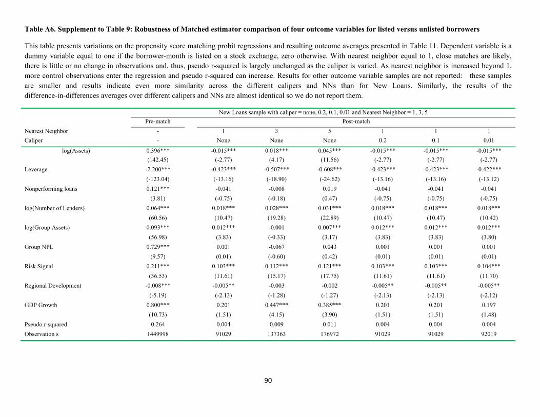
90
Table A6. Supplement to Table 9: Robustness of Matched estimator comparison of four outcome variables for listed versus unlisted borrowers
This table presents variations on the propensity score matching probit regressions and resulting outcome averages presented in Table 11. Dependent variable is a dummy variable equal to one if the borrower-month is listed on a stock exchange, zero otherwise. With nearest neighbor equal to 1, close matches are likely, there is little or no change in observations and, thus, pseudo r-squared is largely unchanged as the caliper is varied. As nearest neighbor is increased beyond 1, more control observations enter the regression and pseudo r-squared can increase. Results for other outcome variable samples are not reported: these samples are smaller and results indicate even more similarity across the different calipers and NNs than for New Loans. Similarly, the results of the difference-in-differences averages over different calipers and NNs are almost identical so we do not report them.
New Loans sample with caliper = none, 0.2, 0.1, 0.01 and Nearest Neighbor = 1, 3, 5
Pre-match Post-match
Nearest Neighbor - 1 3 5 1 1 1
Caliper - None None None 0.2 0.1 0.01
log(Assets) 0.396*** -0.015*** 0.018*** 0.045*** -0.015*** -0.015*** -0.015***
(142.45) (-2.77) (4.17) (11.56) (-2.77) (-2.77) (-2.77)
Leverage -2.200*** -0.423*** -0.507*** -0.608*** -0.423*** -0.423*** -0.422***
(-123.04) (-13.16) (-18.90) (-24.62) (-13.16) (-13.16) (-13.12)
Nonperforming loans 0.121*** -0.041 -0.008 0.019 -0.041 -0.041 -0.041
(3.81) (-0.75) (-0.18) (0.47) (-0.75) (-0.75) (-0.75)
log(Number of Lenders) 0.064*** 0.018*** 0.028*** 0.031*** 0.018*** 0.018*** 0.018***
(60.56) (10.47) (19.28) (22.89) (10.47) (10.47) (10.42)
log(Group Assets) 0.093*** 0.012*** -0.001 0.007*** 0.012*** 0.012*** 0.012***
(56.98) (3.83) (-0.33) (3.17) (3.83) (3.83) (3.80)
Group NPL 0.729*** 0.001 -0.067 0.043 0.001 0.001 0.001
(9.57) (0.01) (-0.60) (0.42) (0.01) (0.01) (0.01)
Risk Signal 0.211*** 0.103*** 0.112*** 0.121*** 0.103*** 0.103*** 0.104***
(36.53) (11.61) (15.17) (17.75) (11.61) (11.61) (11.70)
Regional Development -0.008*** -0.005** -0.003 -0.002 -0.005** -0.005** -0.005**
(-5.19) (-2.13) (-1.28) (-1.27) (-2.13) (-2.13) (-2.12)
GDP Growth 0.800*** 0.201 0.447*** 0.385*** 0.201 0.201 0.197
(10.73) (1.51) (4.15) (3.90) (1.51) (1.51) (1.48)
Pseudo r-squared 0.264 0.004 0.009 0.011 0.004 0.004 0.004
Observation s 1449998 91029 137363 176972 91029 91029 92019
Related Documents


![Architectural categories and acoustic characteristics of ... · Chinese architectural history [2]. Architectural categories and characteristics of tra-ditional Chinese theatres .](https://static.cupdf.com/doc/110x72/6007784cbb3ce4085c1b120d/architectural-categories-and-acoustic-characteristics-of-chinese-architectural.jpg)


