Corn Objective Yield: An Empirical Evaluation

" {~ United States\\ 'I' Department ofAgriculture

NationalAgriculturalStatisticsService

StatisticalResearchDivision

NASS Staff ReportNumber YRB·88-05

June 1986

Corn Objective Yield:An Empirical Evaluationof the Use of 3, 4 or 5Years Data. to DevelopForecast Equations

Ronald J. SteeleBenjamin F. Klugh

CORN OBJECTIVE YIELD: AN EMPIRICAL EVALUATION OF THE USEOF 3, 4 OR 5 YEARS' DATA TO DEVELOP FORECAST EQUATIONS.By Ronald J. Steele and Benjamin F. Klugh, StatisticalResearch Division, National Agricultural StatisticsService, U.S. Department of Agriculture, Washington, D.C.20250, Staff Report No. YRB-Bo-05, June, 19Bo.

ABSTRACT

This study compares the level of forecast errors resultingfrom using data from the previous three, four and five yearsto develop forecast equations for corn yield. Forecast errorsare tabulated for each state and the ten state region in thecorn objective yield program for the years 1980-84. Thesetables provide a benchmark of the performance of the currentcorn objective yield forecast procedures.

Analysis of variance procedures are used to test for signifi-cant differences in the level of forecast errors resultingfrom using different numbers of years of data to estimateregression relationships. The stability of the estimatedregr.ssion parameters is assessed and discussed.

********************************************************** ** This paper was prepared for limited distribution to ** the research community outside the U.S. Department ** of Agriculture. The views expressed herein are not ** necessarily those of NASS or USDA. ** **********************************************************

i

TABLE OF CONTENTS

..............................................SUMMARy •••••• iiiI NTRODUCT I ON ••••••••••••••••••••••••••••••••••••••••••••••••• 1

METHODOLOGY •••••••••••••••••••••••• ~ ••••••••••••••••••••••••. 1

ANALYSIS PROCEDURESForecast Errors •••••••••••••••••Test for Treatment Differences •••••Stability of Parameter Estimates •

·. ... • •3•5

• • 7

..·.RESULTS

Forecast Errors ....................•...Test for Treatment Differences ••Stability of Parameter Estimates ••

·............ • • •91 1

.••••. 12

CONCLUSIONS AND DISCUSSION •••••••••••••••••••••••••••••••.•• 13

RECOMMENOA T IONS ••••••••••••••••••••••••••••••••••••••••••••• 1 4

REFERENCES •••••••••••••••••••••••••••••••••••••••••••••••••• 15

APPENDIX: State-Level Forecast Errors

· .· .Illinois ••••••••••

• 22.23.24.25

•• 26

17• 1819

• • • 20••• 21....·.

·..·....

...· .·..

.....

........

· .

....

.............

·..Indi ana •Iowa •••••Michigan •Minnesota ••Missouri ••Nebraska •••••••••Oh i o •••••South Dakota •Wisconsi n•••••

i i

SUMMARY

For the ten-state region, the average absolute forecast errorfrom 1980 through 1984 across all months is 0.15 bu./acrehigher when five rather than three years' data are used todevelop the forecast equations. This difference for the ten-state region is not statistically significant; neither are thedifferences for individual states.

In general, forecast errors decrease between August and Sep-tember but do not change much between September and October.Forecast errors reported here pertain only to the sampleswhich were not harvested before the end of the survey periodfor that month. Although forecast errors do not decreasebetween September and October, the error in the overallobjective yield estimate does decrease as more samples areharvested.

For the five years included in this study, the forecasts weremore than seven bushels per acre higher than final gross yieldon the average. This upward bias in the forecasts appears tobe due to forecast model insensitivity to weather conditions.Much of this average error is due to overestimating yields in1980 and 1983. In both of these years, yieldS were substan-tially below average due to poor weather conditions.

The estimated parameters of the yield forecast regressionmodels fluctuate considerably from year to year. Increasingthe number of years of data used to estimate the regressionrelationships reduced these fluctuations slightly, but did notimprove the accuracy or reliability of the forecasts for theyears included in this study. Any further increase in thenumber of years of data used will likely decrease the sensi-tivity of the models to changes in cultural practices, agro-nomic technologies, weather and other factors.

iii

CORN OBJECTIVE YIELD. AN EMPIRICAL EVALUATION OF THE USE OF3, 4 OR ~ YEARS· DATA TO DEVELOP FORECAST EQUATIONS

Ronald J. SteeleBenjamin F. Klugh

INTRODUCTION

The National Agricultural Statistics Service (NASS) of theU.S. Department of Agriculture (USDA) conducts monthly CornObjective Yield (COY) surveys from August through November toforecast end-of-season yield of corn for grain for the tenmajor corn producing states. Sample level yield forecasts arecomputed from forecast equations applied to counts and mea-surements made in the sample plots during the current growingseason. The forecast equations are derived by using data fromprevious years' COY surveys to estimate linear relationshipsbetween counts or measurements made during the growing seasonand counts or measurements obtained when the corn is mature.Prior to 1985, the regression relationships were estimatedusing data from the three previous years' surveys. In 1985the procedure was changed; the previous five years' data wereused to develop the forecast equations.

This study examines and compares the forecast errors resultingfrom the use of data from the previous three, four and fiveyears to develop forecast equations for 1980 through 1984.The stability of parameter estimates is also addressed.

METHODOLOGY

- I

A brief description of the COY sampling, dataforecasting methodologies is included here.sive discussions are contained in [7J.

collection andMore comprehen-

Sample units consisting of two plots, each containing two rowsof corn fifteen feet long, are randomly located within a ran-dom sample of fields planted with corn for grain. Counts,measurements and observations of plant characteristics are

1

made within these sample plots during the monthly surveyperiods.When the corn reaches maturity, a count is made of the finalnumber of ears in the sample plots, and the ears are harvestedand weighed. A sample of ears is sent to a laboratory todetermine an adjustment factor for converting field weight tograin weight at 1~.~% moisture. This adjustment factor isapplied to the weight of the ears harvested from the sampleunit, and the result divided by the final number of ears toobtain the final average grain weight per ear. Final grossyield is calculated from the final number of ears, final ave-rage grain weight per ear, and the size of the sample plots.Post-harvest gleaning surveys are conducted to estimate theharvest loss. Estimated harvest loss is subtracted from finalgross yield to obtain final net yield.

With data from the five previous years' COY surveys, simplelinear regression models are used to estimate relationshipsbetween counts (or measurements) obtained during the growingseason and counts made when the corn is mature. Forecasts ofthe final number of ears and average grain weight per ear arecomputed by applying these estimated regression relationshipsto counts and measurements made during the current growingseason. Counts of stalks, stalks with ears, or number of earsare used as the predictor variable for final number of ears,depending on the stage of physiological development (maturitystage). Average kernel row length and average cob length overthe husk are used to predict average grain weight per ear oncethe crop reaches a maturity stage sufficient to make thesemeasurements. A historic average grain weight per ear is usedprior to the development of kernels on ears. The yieldforecast (bushels/acre) is computed by taking the product ofthe forecast number of ears, the forecast grain weight per earand a multiplicative constant, divided by the area in thesample unit. Salient features of the forecasting procedures,beyond those described above, are:

a) generally speaking, forecasts for number of ears andaverage grain weight per ear are each a weighted ave-rage of two forecasts, with weights based on averageR2 values of the estimated regression relationshipsacross maturity categories. In some maturity cate-gories, historic averages or observed data are usedinstead of forecasts from models;

b) regression relationships are estimated using data forthe same state, district, month and maturity categoryfrom the previous years;

2

c) automated outlier/leverage-point detection and removalprocedures are used in developing the forecast equa-tions (3 J ;

d) if there are insufficient data from previous yearswithin some maturity category to estimate the regres-sion relationships, a forecast equation from anothermaturity category, month or year is used. In selectingthe forecast equation to be substituted, equations fromwithin the same month are considered first, then equa-tions from other months, and finally equations fromother years.

e) if the estimated intercept parametermodel is forced through the originIf the slope parameter is negative, ation from another maturity category,substituted following the proceduresabove.

ANALYSIS PROCEDURES

is negative, the(zero intercept).regression equa-month or year isdiscussed in (d)

Forecast Errors

Forecasts and the corresponding forecast errors are computedfor non-mature COY samples for the years 1980 through 1984,with forecast equations developed using COY survey data fromthe previous three, four and five years. The procedures usedto develop the forecast equations and compute the forecastsare essentially the same as are used in the operational COYprogram. For the purposes of this analysis, forecast error isdefined as the difference between the gross yield forecast andthe final gross yield.

Subscripts used in the remainder of this report are:

i denotes treatment: 3, 4 or :5 years' data used todevelop the forecast equations;

j denotes year: j E (1 (1980) , 2 (1981), ... , 5 ( 1984) )

k denotes month: k E < 1 (Aug), 2 (Sept) , 3 (Oct» .,1 denotes state: 1 E <1,2, ••• 10) .,m denotes sample number: m E <1,2, ••• ,nJlcl) •

3

The forecast error for the m~h sample, l~h state,and j~h year, using the i~h treatment, iSI

k~h month

where

is the gross yield forecast for the m~h sample; and

is the final gross yield. It do•• not vary as a func-tion of the month within a year nor the number ofyears of data used to develop the forecast equations.Thus, the i and k subscripts are omitted.

In consideration of the self-weighted sampling plan used inthe COY surveys, we define the state-level forecast error asthe simple mean of the sample-level forecast errors. For thei~h treatment, j~h year, k~h month, and l~h state, the state-level forecast error is:

nJklE1Jk1. = E E1Jk1• I n.tkl

•where

nJkl is the number of samples for which forecasts werecomputed in the j~h year, k~h month, and l~h state. Itdoes not vary as a function of the number of years ofdata used to develop the forecast equations.

The state-level forecast error as defined above excludes theeffect of samples already harvested and samples for which datawere not collected when the corn reached maturity. Samplesalready harvested were excluded since final gross yield isalready observed; the forecast models are no longer used forthese samples in the operational program. The inclusion ofalready harvested samples would only serve to mask any realdifferences which might exist in forecast error levels due tothe numbers of years of data used to develop the forecastequations. Samples for which data were not collected when thecorn reached maturity were excluded through necessity; thefinal gross yield is unknown for those samples, so forecasterrors could not be computed. Some of the reasons data arenot collected when the corn reaches maturity are: the farmerharvests the field before the enumerator is able to harvestthe sample plots; the field is no longer intended to be har-vested as corn for grain; the farm operator reneQes on thepermission granted to enter the field and conduct the survey.

State-level forecast errors are tabulated by month and yearfor the three treatments. The averaoe absolute forecast error

4

and the average squared forecast error are also tabulated foreach month, and for all months combined across the five years.

The average absolute forecast error for the l~h state, k~hmonth, and i~h treatment is:

is the average absoluteforecast error across thethree months.

5:E: •. k1• = t IE'JkI·1 I 5

j=l3

:E:' .. l. = t IEI,.lcl.I 3k=l

and,

Replacing IE'jkl.I with (E'Jlcl.)Z,the average squared fore-cast errors are analogously defined.

Considering the ten-states in the COY survey as a region,regional level forecast errors are also tabulated by month andyear for the three treatments. The regional level forecasterror for the i'h treatment j~h year and k'h month, is definedas the weighted average of the state-level forecast errors:

10E'Jlc.. = t AJ1E'Jlcl.

1=1where

is the final harvested corn for grain acreage, whichdoes not vary with months (k) nor treatments (i); and

is the previously defined state-level forecast errorfor the l'h state, k~h month, j'h year and ithtreatment.

The average absolute forecast error and average squaredforecast error for the ten-state region are defined in thesame manner as the corresponding state-level estimators.

Test for Treatment Differences

Analysis of variance (ANOVA) procedures are used to test fordifferences in the level of forecast errors between treat-ments. Treatments correspond to th. use of data from theprevious three, four or five years to develOp the forecastequations. Although sample sizes are not the same from monthto month nor year to year, we assume that for a given state,the impact of a state-level forecast error of a given

s

magnitude is the same regardless of the month or year in whichit occurs. Under this assumption, unweighted least squares isappropriate. Furthermore, the design is balanced with threetreatments, five years, three months within each year, and oneobservation per cell. All three treatments are applied to thesame set of samples so we effectively have the requisiterAndomization. Treatments, years, and months within years areconsidered fixed effects.

Two dependent variables, or responses, are considered: theabsolute value of the state-level forecast error IE'Jkl. I; andthe squared state-level forecast error (E'Jkl.)2. A separateANOVA is performed for each state. The assumed model for thel~h state (1 fixed), with absolute error as the response, is:

where«, is the effect of the use of three, four or five years

data to develop the forecast equations;

BJ is the effect of the j~h year;

0Jk is the effect of the k~h month within the j~h year; andE'Jkl are assumed to be normal, independent, identically

distributed random variables (1 is fixed).

The model is analogously defined for the squared forecasterror response. The same model is also used for the regionallevel absolute and squared forecast errors, with appropriatemodification of the response variable and assumptions.

The hypothesis of interest is Ho: «1=«2=«3; there is nodifference in the level of the forecast errors due to thenumber of years of data (3, 4 or 5) used. Rejection of thishypothesis will lead to the conclusion that the level of theabsolute (or squared) forecast errors is not the same for alltreatments if the underlying assumptions are satisfied.Hypothesis tests are performed with a testwise type I errorrate of «=.0:5.There are inter-dependencies between treatments since forecastequations based on data from the previous three, four and fiveyears are not independent. Likewise, inter-dependencies existbetween years and months within years. AlthouQh the assumedmodel should largely eliminate these inter-dependencies, theresiduals are examined to assess the validity of the norm-ality, independence and homoscedasticity (equal variance>assumptions.

6

Stability of Parameter EstimatesOne of the primary reasons for changing from the use of threeyears to the use of five years of data to develop the forecastequations was the instability of the parameter estimates. Asa gross, overall measure of the stability of the parameterestimates, a statistic similar to a coefficient of variation(CV> is computed for the intercept and slope parameters ofeach of the four models - two models for final number of ears,and two for average grain weight per ear. We define thismeasure of stability of the estimated parameter p, for thehth parameter of the gth model using the ith treatment (3, 4or 5 years' data> as:

STAB.h, = 100 * ~ lJ'z (6'.h'> I P.h'.... where

P.h' ..••

is the estimated component of variance betweenyears for the hth parameter of the gth model underthe ith treatment; and

is the average parameter estimate across allmaturity categories, state/districts, months andyears, weighted by the number of samples forecastswere computed for using this model. These means areessentially equal for 3, 4 or 5 years', so it has anegligible effect on the measure of stability.

As a computational convenience in estimating the between yearvariance component of an estimated parameter (for a particularmodel, parameter and treatment, with associated g, hand isubscripts omitted for simplicity>, we adopt a nested linearmodel of the form:

where

a_ is the effect of the kth month

B_1 is the effect of the lth state/district within thekth month;

r_l~ is the effect of the qth maturity category withinthe Ith state/district and kth month;

6' _ 1••~ is the effect of thematurity category, Ithmonth;

7

jth year within thestate/district and

is the random error; and

is the parameter estimate for the m~h samplewithin the j~h year, the q~h maturity category,lth state/ district and k~h month.

As a straightforward extension of results presented by Searle[4J for two-way and three-way nested classification models,the analysis of variance estimator of the between-yearcomponent of variance is:

[ttttplkl.Q/nJklQ - tttp~kl'Q/n.klq - (d...- c..)crZ(e»)crZ ( 0 ) = k 1 aj k 1 a

[N-ttttnlklq/n.klQ]k 1 qj

wh er e:

cr2 (e) is the mean squared error from the above model; itsvalue is zero since all samples within a maturitycategory, state/district, month and year have thesame parameter estimate. Specification of the modelwithout the year-term would result in the MSE beingthe ANOVA estimator of the between-year component ofvariance with identical results;

d...- c.. is the degrees of freedom for the between-yearssums of squares;

N is the total number of samples forecasts werecomputed for using estimates of this parameter;

nJk1Q is the number of samples forecasts were computed forusing the estimated parameter for the q~h maturitycateoory, lth state/district, k~h month and jthyear.

The dot subscript notation denotes the customary summationover the indicated subscript.

Caution should be exercised in interpretin; this measure ofstability. As previously defined, '2(8) is a biasedestimate of the variance. The bias arises as a result of thelack of independence in parameter estimates from year to year.Assuming parameter estimates are positively correlated betweenyears within a maturity cateoory, month and state, ~Z(o)will understate the true variance of the parameters. As thenumber of years used to estimate the parameters is increased,

8

this bias will increase substantially unless there is somestrong periodic relationship in the parameter estimates. Itis beyond the scope of this study to develop and computeunbiased estimates of the variance for the parameters.

RESULTS

Forecast Errors

Regional level forecast errors are presented in Table 1.Results for individual states are contained in the Appendix,Tables A-1 through A-10.

There are three notable patterns in the tables. First, withinany month and year, the forecast errors are almost the same,regardless of the number of years used to develop the forecastequations. Second, although there is generally an improvementin the accuracy of the forecasts from August to September,thRre is no substantial gain between September and October.In the operational program, the forecasts do converge towardthe final gross yield in October, but apparently this is dueto the inclusion of data from samples which have already beenharvested. Third, the forecast procedures are upward biased.A preponderance of the forecast errors are positive, and thepositive forecast errors are an order of magnitude larger thanthe negative errors. On the average, forecasts were more thanseven bushels per acre higher than final gross yield. Much ofthis error is due to overestimating yields in 1980 and 1983.Yields were substantially below average during both of theseyears due to poor weather conditions.

These observations are based solely on the data from thesefive years. Extreme care should be exercised in extrapolatingconclusions beyond this time period. Generally speaking, thepatterns observed for the ten-state region also hold for theindividual states.

9

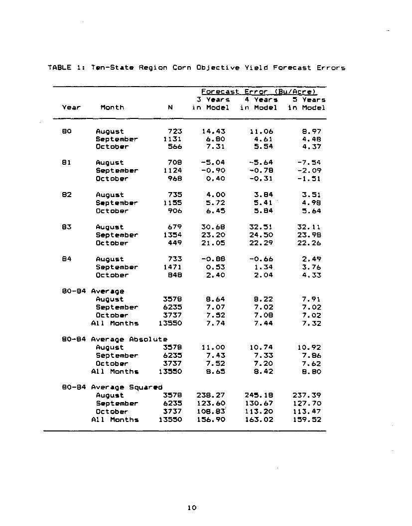
TABLE 1: Ten-State Region Corn Objective Yield Forecast Errors

Forecast Error (Bu/Acre)3 Years 4 Years 5 Years

Year Month N in Model in Model in Model

BO August 723 14.43 11•06 8.97September 1131 6.80 4.61 4.48October 566 7.31 5.54 4.37

81 August 708 -5.04 -5.64 -7.54September 1124 -0.90 -0.78 -2.09October 968 0.40 -0.31 -1.51

82 August 735 4.00 3.84 3.51September 1155 5.72 5.41 4.98October 906 6.45 5.84 5.64

83 August 679 30.68 32.51 32. 11September 1354 23.20 24.50 23.98October 449 2 1.05 22.29 22.26

84 August 733 -0.88 -0.66 2.49September 1471 0.53 1.34 3.76October 848 2.40 2.04 4.33

80-84 AverageAugust 3578 8.64 8.22 7.91September 6235 7.07 7.02 7.02October 3737 7.52 7.08 7.02

All Months 13550 7.74 7.44 7.32

80-84 Average AbsoluteAugust 3578 11.00 10.74 10.92September 6235 7.43 7.33 7.86October 3737 7.52 7.20 7.62

All Months 13550 8.65 8.42 8.8080-84 Average Squared

August 3578 238.27 245.18 237.39September 6235 123.60 130.67 127.70October 3737 108.83' 113.20 113.47

All Months 13550 156.90 163.02 159.52

10

Test for Treatment Differences

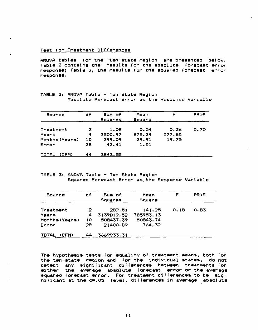
ANOVA tables for the ten-state region are presented below.Table 2 contains the results for the absolute forecast errorresponse; Table 3, the results for the squared forecast errorresponse.

TABLE 2: ANOVA Table - Ten State RegionAbsolute Forecast Error as the Response Variable

Source df Sum of Mean F PR>FSQuares SQuare

Treatment 2 1.08 0.54 0.36 0.70Years 4 3500.97 875.24 577.85Months (Years) 10 299.09 29.91 19.75Error 28 42.41 1.51

TOTAL (CFM) 44 3843.~~

TABLE 3: ANOVA Table - Ten State RegionSquared Forecast Error as.the Response Variable

Source df Sum of MeanSQuares SQuare

Treatment 2 282.51 141.25Years 4 3139812.52 785953.13Months(Years) 10 508437.39 50843.74Error 28 21400.89 764.32

TOTAL (CFM) 44 3669933.31

F

0.18

PR>F

0.83

The hypothesis tests for equality of treatment means, both forthe ten-state region and for the individual states, do notdetect any significant differences between treatments foreither the average absolute forecast error or the averagesquared forecast error. For treatment differences to be sig-nificant at the a=.05 level, differences in average absolute

11

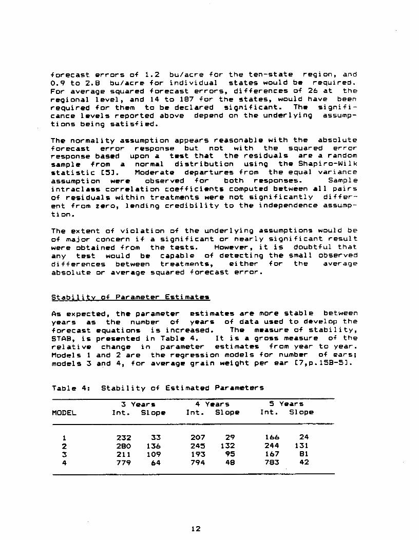
forecast errors of 1.2 bu/acre for the ten-state region, and0.9 to 2.8 bu/acre for individual states would be required.For average squared forecast errors, differences of 26 at theregional level, and 14 to 187 for the states, would have beenrequired for them to be declared significant. The signifi-cance levels reported above depend on the underlying assump-tions being satisfied.

The normality assumption appears reasonable with the absoluteforecast error response but not with the squared errorresponse based upon a test that the residuals are a randomsample from a normal distribution using the Shapiro-Wilkstatistic [5J. Moderate departures from the equal varianceassumption were observed for both responses. Sampleintraclass correlation coefficients computed between all pairsof residuals within treatments were not significantly differ-ent from zero, lending credibility to the independence assump-tion.

The extent of violation of the underlying assumptions would beof major concern if a significant or nearly significant resultwere obtained from the tests. However, it is doubtful thatany test would be capable of detecting the small observeddifferences between treatments, either for the averageabsolute or average squared forecast error.

Stability of Parameter Estimates

As expected, the parameter estimates are more stable betweenyears as the number of years of data used to develop theforecast equations is increased. The measure of stability,STAB, is presented in Table 4. It is a gross measure of therelative change in parameter estimates from year to year.Models 1 and 2 are the regression models for number of ears;models 3 and 4, for average grain weight per ear [7,p.1SB-SJ.

Table 4: Stability of Estimated Parameters

3 Years 4 Years S YearsMODEL Int. Slope Int. Slope Int. Slope

1 232 33 207 29 166 242 280 136 245 132 244 1313 211 109 193 95 167 814 779 64 794 48 783 42

12

Model 2 is not actually a regression model; it is a ratioestimator, the denominator of which is a forecast from anestimated regression relationship. The stability shown abovefor model 2 pertains to the stability of the estimatedparameters for the regression model used in the denominator.

CONCLUSIONS AND DISCUSSION

There is no appreciable difference in the level of forecasterrors when the forecast equations are developed from theprevious three, four or five years' data. In years withaverage or high yields - lQ81, 1982 and 1984 - the forecasterrors are quite reasonable. However, in years with lowyields, especially 1983, the forecast errors are very large.Furthermore, forecast errors do not change much betweenSeptember and October forecasts. These two factors indicatethat the variables being used in the models are not sensitiveto changes in conditions and/or that the models are incorrect,i.e. the relationships being estimated are not the same fromyear to year. There is considerable evidence of the latter,judging from the amount the parameter estimates change fromyear to year.

Changing to the use of five years' data does make theparameter estimates more stable. Changing to the use of 10 or20 years would make them more stable. A logical extensionwould be the use of constant forecast equations, instead ofestimating the parameters each year. The dangers of doingthis should be apparent. If the relationship is not the samefrom year to year, but we force stability in the parameterestimates by increasing the number of years of data used, thelarge positive covariances between years could easily increasethe true variance of the parameter estimates, resulting inless accurate forecasts. In other words, the greater thenumber of years of data used to estimate the forecastequations, the less sensitive the forecast equations will beto changes in crop technologies, weather and other factors.It's important to bear in mind that the purpose of the yieldmodels is not to estimate parameters, but to produce forecastsof yield. Increasing the number of years of data used did notincrease the accuracy of the forecasts for the years includedin this empirical study. This change in procedures onlyserves to mask the the very real problems which exist with thecurrent yield forecast models namely insensitivity toweather and other factors changing between years.

13

RECOMMENDATIONS

The number of years of data used to develop the forecastequations should not be further increased without soundtheoretical or empirical evidence that the accuracy of theforecasts will be improved.

The tables in this report provide a benchmark of the perform-ance of the operational objective yield forecast models. Whensubstantive changes in the operational program are recom-mended, the impact of these changes on the level of the fore-casts should be computed and, when appropriate, comparedagainst this benchmark. Furthermore, the Crop Reporting Boardshould be informed of the level of change in forecasts, orforecast errors, which will result from the proposed change inprocedures.

Development and examination of empirical or theoreticalestimates of the variance/covariance structure of the compo-nents of the sample-level forecasts would shed considerablelight on the major strengths and weaknesses of the currentforecast models. This variance/covariance structure shouldinclude appropriate terms for interactions between estimatedparameters which arise through the use of the multiplicativeyield model. This topic should receive high priority.

Alternative modeling techniques and variables need to beexamined to develop better forecasts. Some techniquescurrently being explored such as production models (lJ,probability models [2J, improved grain weight per ear models[6J, and computer intensive data fitting methods shouldreceive strong emphasis.

14

REFERENCES

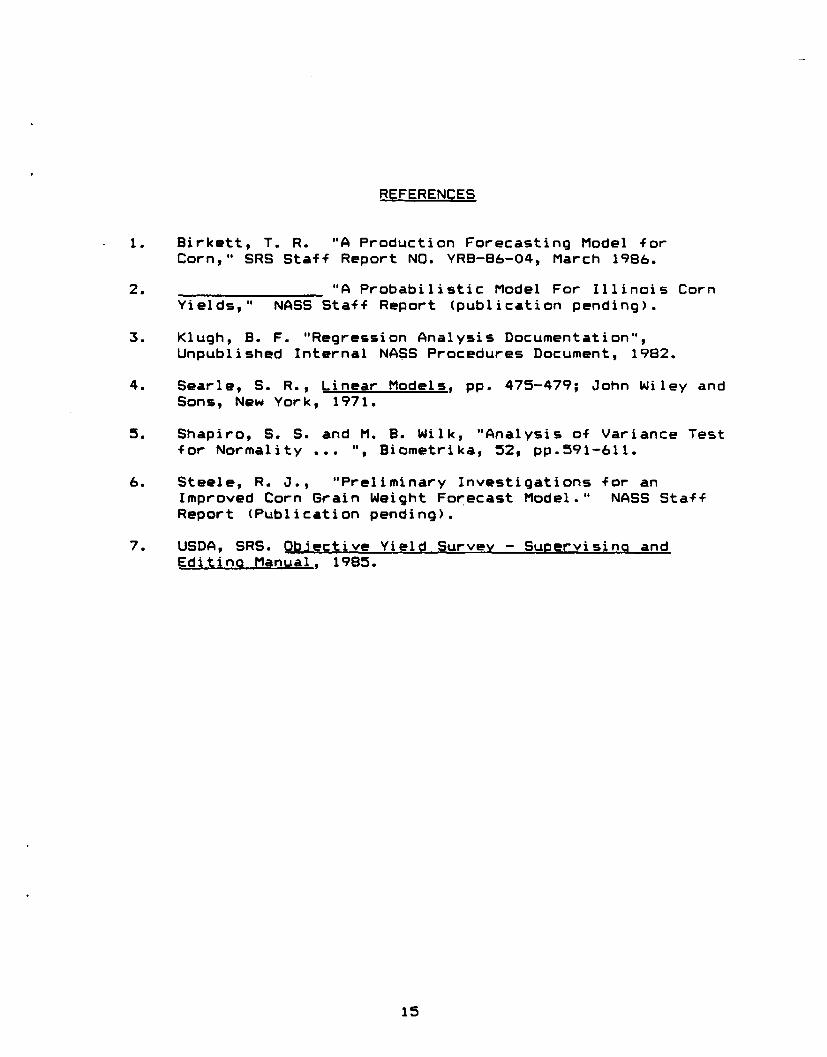
1. Birkett, T. R. "A Production Forecasting Model forCorn," SRS Staff Report NO. YRB-86-04, March 1986.

2. "A Probabilistic Model For Illinois CornYields," NASS Staff Report (publication pending).

3. Klugh, B. F. "Regression Analysis Documentation",Unpublished Internal NASS Procedures Document, 1982.

4. Searle, S. R., Linear Models, pp. 475-479; John Wiley andSons, New York, 1971.

5. Shapiro, S. S. and M. B. Wilk, "Analysis of Variance Testfor Normality ••• ", Biometrika, 52, pp.591-611.

6. Steele, R. J., "Preliminary Investigations for anImproved Corn Grain Weight Forecast Model." NASS StaffReport (Publication pending).

7. USDA, SRS. Objective Yield Survey - Sucervisinc andEditinQ Manual, 1985.

15

TABLE A-l: Illinois Corn Objective Yield Forecast Errors

Forecast Error <Bu/Acre)3 Years 4 Years 5 Years

Year Month N in Model in Model in Mod e1

80 August 108 29.43 29. 14 27.93September 222 10.01 8.36 9.02October 30 16.59 15.75 14.22

81 August 103 -12.86 -13.36 -13.13September 216 -8.90 -9.00 -10.53October 115 -7.10 -8.01 -8.94

82 August 109 8.40 7.04 7.27September 212 2.48 1.36 1.23October 71 9.62 7.~5 7.12

83 August 95 37.52 41.29 40.83September 193 23.38 24.47 23.50October 59 17.52 20.62 20. 12

84 August 111 8.63 6.39 11•64September 222 7.32 6.13 9.57October 92 1.47 0.48 4.81


All Months 1958 9.57 9.21 9.64

80-84 Average AbsoluteAugust 526 19.37 19.44 20.16September 1065 10.42 9.87 10.77October 367 10.46 10.48 11•04

All Months 1958 13.42 13.26 13.99

80-84 Averagll SquaredAugust 526 516.79 564.55 561. 62September 1065 157 •18 157.82 167.53October 367 145.52 158.94 152. 13 ;

All Months 1958 273. 16 293.77 293.76

17

TABLE A-2: Indiana Corn Objective Yield Forecast Errors


Year Month N in Model in Model in Mod eI


81 August 85 -6.42 -5.68 -5.11September 162 -0.69 -0.34 -3.20October 135 0.82 -0.38 -0.44


83 August 76 40.66 41.77 41 •26September 155 21 •25 22.60 23.08October 42 22. 10 22. 18 22.34


80-84 AverageAugust 410 S.10 5.37 5.76September 828 1.80 2.15 2.18October 359 2.14 1.33 1.53

All Months 1597 3.01 2.95 3.16

80-84 Average AbsoluteAugust 410 16.35 16.67 15.01September 828 10.29 10.46 10.73October 359 11.40 11•87 11.54

All Months 1597 12.68 13.00 12.43

80-84 Average SquaredAugust 410 421. 21 443.26 401. 52Sept limber 828 150.65 163.36 1'59.22October 359 176.09 193.30 183.21

All Months 1597 249.32 266.64 247.98

18

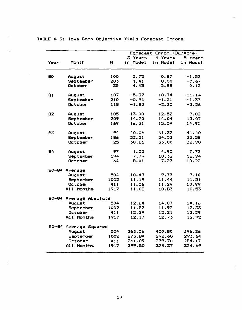
TABLE A-3: Iowa Corn Objective Yield Forecast Errors



80 August 100 3.73 0.87 -1 •52September 203 1.41 0.00 -0.67October 35 4.45 2.88 0.12

81 August 107 -5.37 -10.74 -11. 14September 210 -0.94 -1.21 -1.37October 118 -1.82 -2.30 -3.26




80-84 AverageAugust 504 10.49 9.77 9.10September 1002 11.19 11.44 11.51October 411 11•56 11•29 10.99

All Months 1917 11•08 10.83 10.53

80-84 Average AbsoluteAugust 504 12.64 14.07 14.16September 1002 11•57 11.92 12.33October 411 12.29 12.21 12.29

All Months 1917 12.17 12.73 12.92

80-84 Average SquaredAugust 504 363.56 400.80 396.26September 1002 273.84 292.60 293.b4October 411 261. 09 279.70 284.17

All Months 1917 299.50 324.37 324.69

19

TABLE A-4: Michigan Corn Objective Yield Forecast Errors



80 August 47 0.70 -3.05 -4.11September 47 2.99 0.84 1.35October 90 0.85 -2.86 -3.45

81 August 42 -0.63 0.56 -2.52September 42 2.29 1.97 -0.33October 64 2.38 2.53 0.26

B2 August 46 -4.77 -6.72 -5.52September 46 2.32 3.45 1.92October 71 2.71 2.28 2.23

83 August 40 7.00 7.66 5.73September 77 10.23 11.75 10.15Octobltr 59 8.44 8.85 8.00

84 August 43 19.97 20.88 21. 87Septltmber 84 10.77 11.60 12.98October 63 8.37 9.12 10.37


All Months 861 4.91 4.59 3.93


All Months 861 5.63 6.28 6.05

80-84 Average SquaredAugust 218 94.26 109.86 112.99September 296 48.04 37.83 55.40October 347 31.00 36.23 37.69

All Months 861 57.77 67.97 68.70

20

TABLE A-~: Minnesota Corn Objective Yield Forecast Errors

Forecast Error (Bu/Acre)3 Years 4 Years ~ Years


80 August 78 3.19 -4.30 -7.05September 147 -0.74 -2.82 -2.91October 121 -5.37 -6.42 -5.77


82 August 70 -3.57 -2.60 -1.35September 148 -1.24 -1.33 -1.45October 134 0.09 -0.06 0.06

83 August 60 31.47 28.82 29.33September 134 2~.89 24.37 24.24October 64 18.48 16.47 16.24


80-84 AverageAugust 356 ~.04 3.67 2.41September 725 4.09 3.52 3.19October 567 3.87 3.59 3.40

All Months 1648 4.37 3.59 3.00


All Months 1648 7.~5 7.50 7.85

80-84 Average SquaredAugust 356 216.44 182.79 210.67September 725 137.72 124.40 124.81October ~67 85.69 78.27 71. 61

All Months 1648 146.62 128.49 135.70

21

TABLE A-6: Missouri Corn Objective Yield Forecast Errors


Year Month N in Model in Model in Mod e 1

80 August 47 38.64 33.03 31 .04September 78 14.72 12.40 10.08October 3 2:5.04 21.85 20.55

81 August 48 -31. 82 -30.45 -30.41September 104 -16.27 -16.31 -17.92October 17 3.61 -0.87 -2.94



84 August 57 :5.57 -1. 17 6.92September 108 11•88 8.90 15.64October 19 8.98 8.00 13.28

80-84 AverageAugust 266 12.83 12.65 13.06September 482 10.08 9.53 9.54October 75 14.28 11•39 12.02

All Months 823 12.40 11.19 11•54


All Months 823 18.81 17.70 18.38

80-84 Average SquarttdAugust 266 870.63 986.13 959.39September 482 317.66 332.31 346.37October 75 258.17 186.61 209.17

All Months 823 482.15 501.68 504.98

22

TABLE A-7: Nebraska Corn Objective Yield Forecast Errors


Yea.r Month N in Model in Model in Model


81 August 88 -1.27 0.84 -5.45September 89 1.99 3.70 0.73October 105 4.88 3.84 -0.09


83 August 94 20.85 24.15 26.76September 187 17.63 22.14 21 •35October 20 32.46 35.24 35.35

84 AUQust 94 -5.50 -10.57 -5.61September 183 -4.29 -3.92 -0.78October 75 3.85 3.32 6.36


All Months 1442 11•62 10.97 10.89


All Months 1442 13.09 12.90 12.49

80-84 Average SquaredAugust 442 384.56 320.59 316.63September 626 221.90 200.42 190.51October 374 288.42 305.40 308.67

All Months 1442 298.30 275.47 271.93

23

TABLE A-8: Ohio Corn Objective Yield Forecast Errors

Year Month N

Forecast Error <Bu/Acre)3 Years 4 Years 5 Years

in Model in Modlll in Model

80 AugustSeptemberOctober

81 AUQustSeptemberOctober




80-84 AveraQeAugustSeptemberOctober

All Months

727343

6666

120

798055

7415151

75148112

366518381

1265

-0.265.484.57

18.0918.1314.11

1.535.39

-10.14

24.8420.756.32

-21. 98-21.46-11.00

4.445.660.773.62

0.675.964.87

19.4018.7115.07

2.927.04

-8.65

23.5921 •896.65

-16.97-17.97-10.26

5.927.131.534.86

-2.2993.853.90

20.6519.5215.97

3.236.84

-7.32

24.2222.24

7.28

-14.96-15.87-9.78

6.177.322.015.17

80-84 AveraQe AbsoluteAUQust 366September 518October 381

All Months 1265

13.3414.249.23

12.27

12.7114.319.10

12.04

13.0713.668.85

11.86

80-84 AveraQIt SquaredAUQustSltptllmbllrOctober

All Months

366518381

1265

24

285.87255.8196.75

212.81

245.97247.3995.03

196.13

250.60237.7894.54

194.31

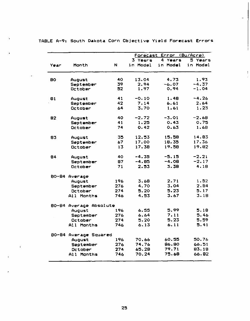
TABLE A-9: South Dakota Corn Objective Yield Forecast Errors



80 August 40 13.04 4.73 1.93September 39 2.94 -6.07 -4.37October 52 1.97 0.94 - 1•04

81 August 41 -0.10 1.48 -4.26September 42 7.14 6.61 2.64October 64 3.70 1.61 1.23

82 August 40 -2.72 -3.01 -2.68September 41 1.25 0.43 0.75October 74 0.42 0.63 1.68

83 August 35 12.53 15.58 14.83September b7 17.00 18.35 17.36October 13 17.38 19.58 19.82

84 August 40 -4.35 -5.15 -2.21September 87 -4.85 -4.08 -2.17October 71 2.53 3.38 4.18

80-84 AverageAugust 196 3.68 2.71 1.S2September 276 4.70 3.04 2.84October 274 5.20 5.23 S.17

All Months 746 4.53 3.67 3.18

80-84 Average AbsoluteAugust 196 6.55 5.99 S.18September 276 6.64 7.11 5.46October 274 5.20 5.23 5.59

All Months 746 6.13 6.11 5.41

80-84 Average SquaredAugust 196 70.6b 60.55 50.76September 276 74.76 86.80 66.51October 274 65.28 79.71 83.18

All Months 746 70.24 75.68 66.82

25

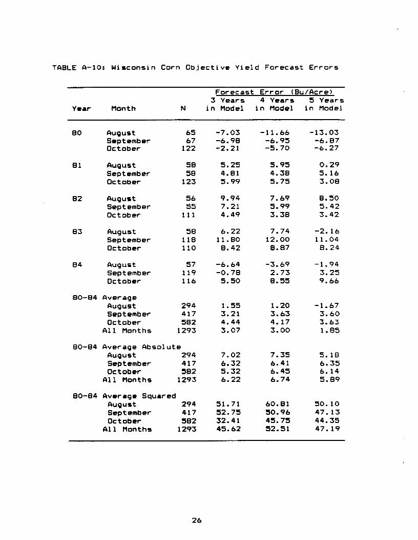
TABLE A-I0: Wisconsin Corn Objective Yield Forecast Errors

Forecast Error (Bu/Acre>3 Years 4 Years ~ Years





83 August 58 6.22 7.74 -2.16September 118 11.80 12.00 11.04October 110 8.42 8.87 8.24

84 August 57 -6.64 -3.69 -1.94September 119 -0.78 2.73 3.25October 116 5.50 8.55 9.66

80-84 AverageAugust 294 1.55 1.20 -1. 67September 417 3.21 3.63 3.60October 582 4.44 4.17 3.63

All Months 1293 3.07 3.00 1.85


All Months 1293 6.22 6.74 5.89

80-84 Average SquaredAugust 294 51.71 60.81 50.10September 417 52.75 50.96 47.13Octobltr ~82 32.41 45.75 44.35

All Months 1293 45.62 ~2.51 47. 19

26

Corn Objective Yield: An Empirical Evaluation

Documents