Cords: geometric curve primitives for modeling contact

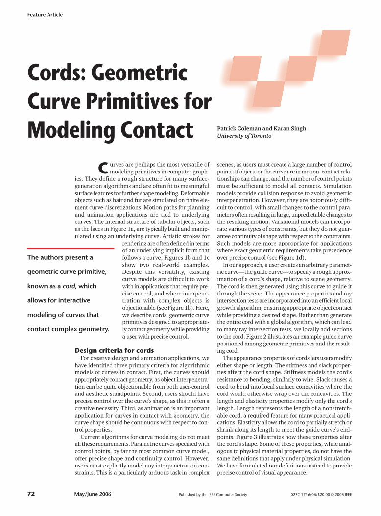
C urves are perhaps the most versatile ofmodeling primitives in computer graph-

ics. They define a rough structure for many surface-generation algorithms and are often fit to meaningfulsurface features for further shape modeling. Deformableobjects such as hair and fur are simulated on finite ele-ment curve discretizations. Motion paths for planningand animation applications are tied to underlyingcurves. The internal structure of tubular objects, suchas the laces in Figure 1a, are typically built and manip-ulated using an underlying curve. Artistic strokes for

rendering are often defined in termsof an underlying implicit form thatfollows a curve; Figures 1b and 1cshow two real-world examples.Despite this versatility, existingcurve models are difficult to workwith in applications that require pre-cise control, and where interpene-tration with complex objects isobjectionable (see Figure 1b). Here,we describe cords, geometric curveprimitives designed to appropriate-ly contact geometry while providinga user with precise control.

Design criteria for cordsFor creative design and animation applications, we

have identified three primary criteria for algorithmicmodels of curves in contact. First, the curves shouldappropriately contact geometry, as object interpenetra-tion can be quite objectionable from both user-controland aesthetic standpoints. Second, users should haveprecise control over the curve’s shape, as this is often acreative necessity. Third, as animation is an importantapplication for curves in contact with geometry, thecurve shape should be continuous with respect to con-trol properties.

Current algorithms for curve modeling do not meetall these requirements. Parametric curves specified withcontrol points, by far the most common curve model,offer precise shape and continuity control. However,users must explicitly model any interpenetration con-straints. This is a particularly arduous task in complex

scenes, as users must create a large number of controlpoints. If objects or the curve are in motion, contact rela-tionships can change, and the number of control pointsmust be sufficient to model all contacts. Simulationmodels provide collision response to avoid geometricinterpenetration. However, they are notoriously diffi-cult to control, with small changes to the control para-meters often resulting in large, unpredictable changes tothe resulting motion. Variational models can incorpo-rate various types of constraints, but they do not guar-antee continuity of shape with respect to the constraints.Such models are more appropriate for applicationswhere exact geometric requirements take precedenceover precise control (see Figure 1d).

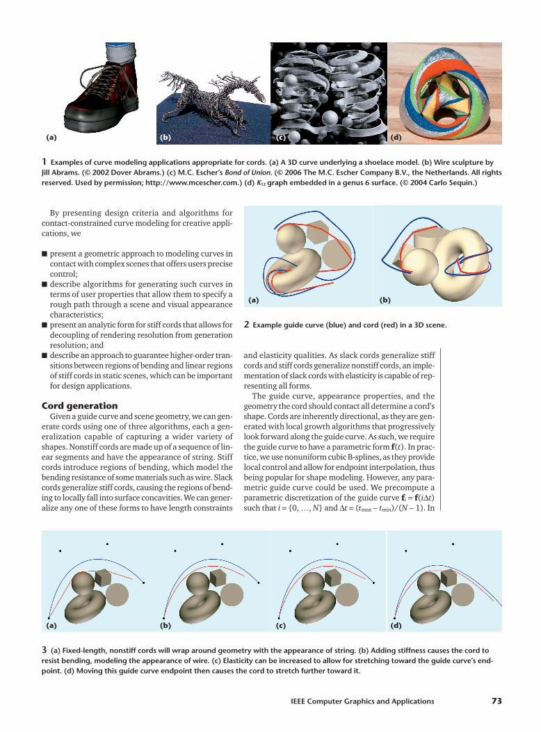
In our approach, a user creates an arbitrary paramet-ric curve—the guide curve—to specify a rough approx-imation of a cord’s shape, relative to scene geometry.The cord is then generated using this curve to guide itthrough the scene. The appearance properties and rayintersection tests are incorporated into an efficient localgrowth algorithm, ensuring appropriate object contactwhile providing a desired shape. Rather than generatethe entire cord with a global algorithm, which can leadto many ray intersection tests, we locally add sectionsto the cord. Figure 2 illustrates an example guide curvepositioned among geometric primitives and the result-ing cord.

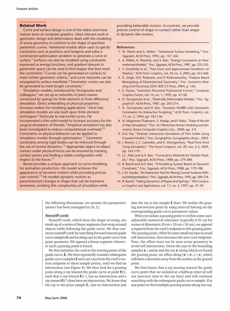
The appearance properties of cords lets users modifyeither shape or length. The stiffness and slack proper-ties affect the cord shape. Stiffness models the cord’sresistance to bending, similarly to wire. Slack causes acord to bend into local surface concavities where thecord would otherwise wrap over the concavities. Thelength and elasticity properties modify only the cord’slength. Length represents the length of a nonstretch-able cord, a required feature for many practical appli-cations. Elasticity allows the cord to partially stretch orshrink along its length to meet the guide curve’s end-points. Figure 3 illustrates how these properties alterthe cord’s shape. Some of these properties, while anal-ogous to physical material properties, do not have thesame definitions that apply under physical simulation.We have formulated our definitions instead to provideprecise control of visual appearance.

Feature Article

The authors present a

geometric curve primitive,

known as a cord, which

allows for interactive

modeling of curves that

contact complex geometry.

Patrick Coleman and Karan SinghUniversity of Toronto

Cords: GeometricCurve Primitives forModeling Contact

72 May/June 2006 Published by the IEEE Computer Society 0272-1716/06/$20.00 © 2006 IEEE

By presenting design criteria and algorithms for contact-constrained curve modeling for creative appli-cations, we

■ present a geometric approach to modeling curves incontact with complex scenes that offers users precisecontrol;

■ describe algorithms for generating such curves interms of user properties that allow them to specify arough path through a scene and visual appearancecharacteristics;

■ present an analytic form for stiff cords that allows fordecoupling of rendering resolution from generationresolution; and

■ describe an approach to guarantee higher-order tran-sitions between regions of bending and linear regionsof stiff cords in static scenes, which can be importantfor design applications.

Cord generationGiven a guide curve and scene geometry, we can gen-

erate cords using one of three algorithms, each a gen-eralization capable of capturing a wider variety ofshapes. Nonstiff cords are made up of a sequence of lin-ear segments and have the appearance of string. Stiffcords introduce regions of bending, which model thebending resistance of some materials such as wire. Slackcords generalize stiff cords, causing the regions of bend-ing to locally fall into surface concavities. We can gener-alize any one of these forms to have length constraints

and elasticity qualities. As slack cords generalize stiffcords and stiff cords generalize nonstiff cords, an imple-mentation of slack cords with elasticity is capable of rep-resenting all forms.

The guide curve, appearance properties, and thegeometry the cord should contact all determine a cord’sshape. Cords are inherently directional, as they are gen-erated with local growth algorithms that progressivelylook forward along the guide curve. As such, we requirethe guide curve to have a parametric form f(t). In prac-tice, we use nonuniform cubic B-splines, as they providelocal control and allow for endpoint interpolation, thusbeing popular for shape modeling. However, any para-metric guide curve could be used. We precompute aparametric discretization of the guide curve fi = f(iΔt)such that i = {0, …, N} and Δt = (tmax − tmin)/(N − 1). In

IEEE Computer Graphics and Applications 73

1 Examples of curve modeling applications appropriate for cords. (a) A 3D curve underlying a shoelace model. (b) Wire sculpture byJill Abrams. (© 2002 Dover Abrams.) (c) M.C. Escher’s Bond of Union. (© 2006 The M.C. Escher Company B.V., the Netherlands. All rightsreserved. Used by permission; http://www.mcescher.com.) (d) K12 graph embedded in a genus 6 surface. (© 2004 Carlo Sequin.)

2 Example guide curve (blue) and cord (red) in a 3D scene.

(a) (b) (c) (d)

(a) (b)

3 (a) Fixed-length, nonstiff cords will wrap around geometry with the appearance of string. (b) Adding stiffness causes the cord toresist bending, modeling the appearance of wire. (c) Elasticity can be increased to allow for stretching toward the guide curve’s end-point. (d) Moving this guide curve endpoint then causes the cord to stretch further toward it.

(a) (b) (c) (d)

the following discussions, we assume the parameteri-zation t has been remapped to [0, 1].

Nonstiff cordsNonstiff cords, which have the shape of string, are

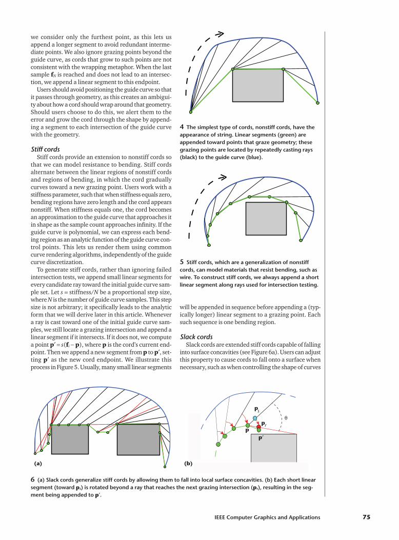
made up of a series of linear segments that wrap aroundobjects while following the guide curve. We thus con-struct nonstiff cords by searching forward toward guidecurve samples fi and locating rays to the guide curve thatgraze geometry. We append a linear segment whenev-er such a grazing point is found.

We first initialize the cord to the starting point of theguide curve, f0. We then repeatedly consider subsequentguide curve samples fi and cast rays from the cord’s cur-rent endpoint to these sample points, until we find anintersection (see Figure 4). We then look for a grazingpoint along a ray toward the guide curve at point f(t),such that a ray toward f(t−), has no intersection and aray toward f(t+) does have an intersection. We know thatthe ray to the prior sample fi-1 has no intersection and

that the ray to the sample fi does. We isolate the graz-ing intersection point by using interval halving on thecorresponding guide curve parameter values.

When we isolate a grazing point to within some user-adjustable numerical tolerance (typically 0.01 cm forscenes of dimension 10 cm × 10 cm × 10 cm), we appenda segment from the cord’s endpoint to this grazing point.The grazing point, offset by some small ray bias to avoidself-intersection, then becomes the new cord endpoint.Note, the offset must not be near scene geometry toavoid self-intersection. Given the rays to the boundingsamples ri-1 and ri and the ray rt along which we foundthe grazing point, we offset along (ri × ri-1) × rt, whichwill have a direction away from the surface at the grazedpoint.

We then know that a ray moving toward the guidecurve point that we isolated at a halfway interval willnot intersect (due to the ray bias) and will continuesearching with the subsequent guide curve sample. If atany point we find multiple grazing points along one ray,

Feature Article

74 May/June 2006

Related WorkCurve and surface design is one of the oldest and most

mature areas of computer graphics. Most relevant work ingeometric design and deformation deals with the modelingof scene geometry to conform to the shape of specifiedparametric curves. Variational models allow users to specifyconstraints such as positions and tangents and solve aconstrained optimization problem to generate a curve orsurface.1 Surfaces can also be modeled using constraintsexpressed as energy functions, and gradient descent inparameter space can be used to find shapes that best meetthe constraints.2 Curves can be generated on surfaces tomeet certain geometric criteria,3 and curve networks can beretargeted to surface manifolds.4 Parametric curves can alsobe generated to meet length constraints.5

Simulation models, introduced by Terzopoulos andcolleagues,6 are set up as networks of point massesconnected by springs for finite element or finite differencesimulation. Direct embedding of physical propertiesincreases realism for modeling applications.7 Most hairsimulation models are also built upon finite elementtechniques.8 Particular to real-world curves, Paiincorporated a thin-solid model to increase accuracy for thesurgical simulation of threads.9 Empirical simulation has alsobeen investigated to reduce computational overhead.10

Constraints on physical behavior can be applied tosimulation models through optimization.11 Geometricconstraints among rigid bodies can be enforced throughthe use of inverse dynamics.12 Appropriate object-to-objectcontact under physical forces can be ensured by trackingcontact points and finding a stable configuration withrespect to the forces.13

Barzel provides a unique approach to curve modelingfor animation production. His model achieves theappearance of dynamic motion while providing preciseuser control.14 He models dynamic motion asparameterized changes in shape that can be keyframeanimated, avoiding the complexities of simulation while

providing believable motion. In contrast, we provideprecise control of shape in contact rather than shape in dynamic-like motion.

References1. W. Welch and A. Witkin, “Variational Surface Modeling,” Proc.

Siggraph, ACM Press, 1992, pp. 157-166.2. A. Witkin, K. Fleischer, and A. Barr, “Energy Constraints on Para-

meterized Models,” Proc. Siggraph, ACM Press, 1987, pp. 225-232.3. V. Surazhsky et al., “Fast Exact and Approximate Geodesics on

Meshes,” ACM Trans. Graphics, vol. 24, no. 3, 2005, pp. 553-560.4. K. Singh, H.K. Pedersen, and D Krishnamurthy, “Feature Based

Retargeting of Parameterized Geometry,” Proc. Geometric Mod-eling and Processing 2004, IEEE CS Press, 2004, p. 163.

5. E. Fiume, “Isometric Piecewise Polynomial Curves,” ComputerGraphics Forum, vol. 14, no. 1, 1995, pp. 47-58.

6. D. Terzopoulos et al., “Elastically Deformable Models,” Proc. Sig-graph 87, ACM Press, 1987, pp. 205-214.

7. D. Terzopoulos and H. Qin, “Dynamic NURBS with GeometricConstraints for Interactive Sculpting,” ACM Trans. Graphics, vol.13, no. 2, 1994, pp. 103-136.

8. N. Magnenat-Thalmann, S. Hadap, and P. Kalra, “State of the Artin Hair Simulation,” Proc. Int’l Workshop Human Modeling and Ani-mation, Korea Computer Graphics Soc., 2000, pp. 3-9.

9. D.K. Pai, “Strands: Interactive Simulation of Thin Solids UsingCosserat Models,” Proc. Eurographics, Eurographics Assoc., 2002.

10. J. Brown, J.-C. Latombe, and K. Montgomery, “Real-Time KnotTying Simulation,” The Visual Computer, vol. 20, nos. 2-3, 2004,pp. 165-179.

11. J.C. Platt and A.H. Barr, “Constraints Methods for Flexible Mod-els,” Proc. Siggraph, ACM Press, 1988, pp. 279-288.

12. R. Barzel and A.H. Barr, “A Modeling System Based on DynamicConstraint,” Proc. Siggraph, ACM Press, 1988, pp. 179-188.

13. J. M. Snyder, “An Interactive Tool for Placing Curved Surfaces With-out Interpenetration,” Proc. Siggraph, ACM Press, 1995, pp. 209-218.

14. R. Barzel, “Faking Dynamics of Ropes and Springs,” IEEE Comput-er Graphics and Applications, vol. 17, no. 3, 1997, pp. 31-39.

we consider only the furthest point, as this lets usappend a longer segment to avoid redundant interme-diate points. We also ignore grazing points beyond theguide curve, as cords that grow to such points are notconsistent with the wrapping metaphor. When the lastsample fN is reached and does not lead to an intersec-tion, we append a linear segment to this endpoint.

Users should avoid positioning the guide curve so thatit passes through geometry, as this creates an ambigui-ty about how a cord should wrap around that geometry.Should users choose to do this, we alert them to theerror and grow the cord through the shape by append-ing a segment to each intersection of the guide curvewith the geometry.

Stiff cordsStiff cords provide an extension to nonstiff cords so

that we can model resistance to bending. Stiff cordsalternate between the linear regions of nonstiff cordsand regions of bending, in which the cord graduallycurves toward a new grazing point. Users work with astiffness parameter, such that when stiffness equals zero,bending regions have zero length and the cord appearsnonstiff. When stiffness equals one, the cord becomesan approximation to the guide curve that approaches itin shape as the sample count approaches infinity. If theguide curve is polynomial, we can express each bend-ing region as an analytic function of the guide curve con-trol points. This lets us render them using commoncurve rendering algorithms, independently of the guidecurve discretization.

To generate stiff cords, rather than ignoring failedintersection tests, we append small linear segments forevery candidate ray toward the initial guide curve sam-ple set. Let s = stiffness/N be a proportional step size,where N is the number of guide curve samples. This stepsize is not arbitrary; it specifically leads to the analyticform that we will derive later in this article. Whenevera ray is cast toward one of the initial guide curve sam-ples, we still locate a grazing intersection and append alinear segment if it intersects. If it does not, we computea point p′ = s(fi − p), where p is the cord’s current end-point. Then we append a new segment from p to p′, set-ting p′ as the new cord endpoint. We illustrate thisprocess in Figure 5. Usually, many small linear segments

will be appended in sequence before appending a (typ-ically longer) linear segment to a grazing point. Eachsuch sequence is one bending region.

Slack cordsSlack cords are extended stiff cords capable of falling

into surface concavities (see Figure 6a). Users can adjustthis property to cause cords to fall onto a surface whennecessary, such as when controlling the shape of curves

IEEE Computer Graphics and Applications 75

4 The simplest type of cords, nonstiff cords, have theappearance of string. Linear segments (green) areappended toward points that graze geometry; thesegrazing points are located by repeatedly casting rays(black) to the guide curve (blue).

5 Stiff cords, which are a generalization of nonstiffcords, can model materials that resist bending, such aswire. To construct stiff cords, we always append a shortlinear segment along rays used for intersection testing.

p

s

p

p’

r

p

θ

6 (a) Slack cords generalize stiff cords by allowing them to fall into local surface concavities. (b) Each short linearsegment (toward ps) is rotated beyond a ray that reaches the next grazing intersection (pr), resulting in the seg-ment being appended to p′.

(a) (b)

on surfaces. We define a slack property, such that whenslack is zero, the cord otherwise behaves like a stiff cord.If slack is one, the cord will have a sagging appearance.If slack is sufficiently greater than one, it will generatea cord that lies close to the surface in regions of localconcavity. If stiffness is zero, slack has no effect on thecord’s shape.

We modify the stiff cord algorithm so that the smalllinear segments of bending regions grow in an altogeth-er different direction. As with stiff cords, we calculate aproportional step point ps, in the direction of the guidecurve sample (blue in Figure 6b). Additionally, the algo-rithm finds the next grazing ray (red). We then calcu-late a step along that ray that is equal in length to thestep toward the guide curve sample (the red point, pr).We calculate the new cord point p′ as a rotational inter-polation or extrapolation from ps to pr. The slack para-meter parameterizes this interpolation, so that if theangle from ps − p to pr − p is θ, the angle from ps − p top′ − p is slack ∗ θ. If p′ should cause the cord to passthrough the surface, it is truncated at the intersectionpoint.

If slack is sufficiently large, the cord will lie in the con-vex regions of a surface that it would otherwise wrapover. Slack is also not appropriate for large, near-closedconcave regions and will not appropriately move to liein the surface that is internal to them, as this can beambiguous. Instead, the slack cords handle subtle con-cavities as would appear in a bumpy surface, where userintent is clear. Regions of bending in slack cords do notadmit an analytic form, as each proportional step incor-porates ray intersection tests that are often discontinu-ous with respect to a parameterization.

Length constraints and elasticityThe nonstiff, stiff, and slack cords interpolate both

guide curve endpoints. Often, we want to enforce lengthconstraints along a curve to model materials with vari-ous stretching properties. It’s also useful to allow a cordto stretch or shrink as the guide curve stretches orshrinks, without necessarily interpolating its endpoints.We allow users to modify properties of length and elas-ticity to accomplish this. Rather than physically model

elasticity and its effect on the cord’s shape, which wouldbe difficult to control, we use elasticity to stretch orshrink the cord only along its length. This decouplingallows users to more easily animate cords in a keyframeenvironment, one of our target applications. We alsomodel elasticity so that when its value is zero, the cordhas a fixed length equal to the length property. Whenelasticity is one, these properties have no effect on theappearance, and the cord interpolates both endpointsof the guide curve. We constrain elasticity to have avalue in [0, 1].

We first generate a cord using any of the previouslydescribed algorithms; let its length be lc. We then computea target length lt = elasticity ∗ lc + (1 − elasticity) ∗ length,an interpolation between the length of a cord interpolat-ing both endpoints and the length appearance property.If lt < lc, we simply truncate the cord to the target length.If lt > lc, we extend the cord along its end tangent, addinga linear segment of length lt − lc. This constrains the gen-erated cord relative to one endpoint of the guide curve.To constrain to a general position along the guide curve,we could apply the truncation or extension to both ends ofthe cord. Figure 7 illustrates the use of cords with zeroelasticity whose length has been animated.

Analytic extensionsThe algorithms we just described generate cords effi-

ciently, are easy to code, and capture the desired designproperties. For stiff cords, however, we can improveupon these algorithms while generating the sameshapes. First, we generate the bending regions of stiffcords as sequences of small linear segments. We willderive an analytic form for these bending regions, whichallows their continuity properties to be expressed interms of the guide curve’s continuity properties. Userscan then achieve desired continuity properties by usingan appropriate form for the guide curve. This analyticform also allows rendering of stiff cords at a resolutionindependent of the guide curve discretization. In addi-tion, for polynomial guide curves specified with controlpoints or other geometric constraints, we can analyti-cally compute the bending regions using only the guidecurve control points.

Feature Article

76 May/June 2006

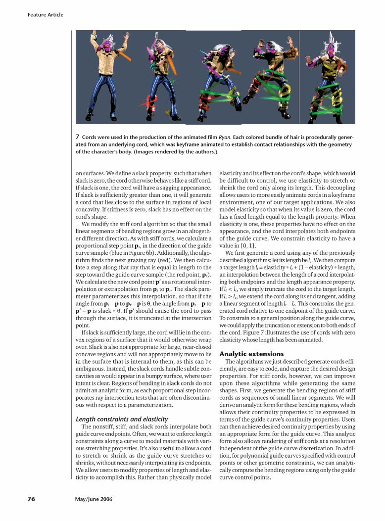
7 Cords were used in the production of the animated film Ryan. Each colored bundle of hair is procedurally gener-ated from an underlying cord, which was keyframe animated to establish contact relationships with the geometryof the character’s body. (Images rendered by the authors.)

Stiff cords possess tangent continuity at join pointsbetween bending regions and linear segments. Somedesign applications require higher-order continuity atjoin points. Here we describe an approach to replacingthe linear regions of nonanimated stiff cords with quin-tic spans, so that the entire cord is G2 continuous.

These extensions don’t apply to slack cords, as slackcords can have arbitrary discontinuities due to the incor-poration of the grazing ray direction into every cord segment.

Stiff cords: regions of bendingRegions of bending for nonslack cords converge to an

analytic form as the number of guide curve samplesapproaches infinity. Given an analytic form, if the guidecurve is a polynomial specified with control points, wecan express the regions of bending in terms of the guidecurve control points. Without loss of generality, let thestart of a bending region be some point p0. We can thinkof this point as generated by some ray cast to a guidecurve point f(t0). Similarly, the last point in the bend-ing region is generated by a ray to f(t1). Without loss ofgenerality, let t0 = 0 and t1 = 1.

Recall, from the definition of stiffness in the “Stiffcords” section, that s = stiffness Δt. We can write a sin-gle step of the generation algorithm in the form

pi = pi-1 + aΔt (f (iΔt) − pi-1)

using a as shorthand notation for stiffness. Dividing byΔt and taking the limit as Δt → 0, we arrive at the fol-lowing differential equation involving the bendingregion g(t):

(1)

This is a first-order differential equation, and given theinitial condition g(0) = p0, it has the solution

(2)

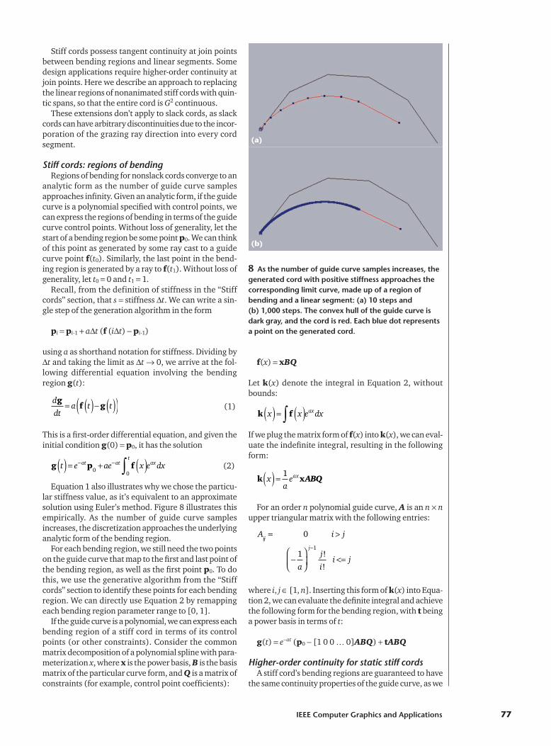
Equation 1 also illustrates why we chose the particu-lar stiffness value, as it’s equivalent to an approximatesolution using Euler’s method. Figure 8 illustrates thisempirically. As the number of guide curve samplesincreases, the discretization approaches the underlyinganalytic form of the bending region.

For each bending region, we still need the two pointson the guide curve that map to the first and last point ofthe bending region, as well as the first point p0. To dothis, we use the generative algorithm from the “Stiffcords” section to identify these points for each bendingregion. We can directly use Equation 2 by remappingeach bending region parameter range to [0, 1].

If the guide curve is a polynomial, we can express eachbending region of a stiff cord in terms of its controlpoints (or other constraints). Consider the commonmatrix decomposition of a polynomial spline with para-meterization x, where x is the power basis, B is the basismatrix of the particular curve form, and Q is a matrix ofconstraints (for example, control point coefficients):

f(x) = xBQ

Let k(x) denote the integral in Equation 2, withoutbounds:

If we plug the matrix form of f(x) into k(x), we can eval-uate the indefinite integral, resulting in the followingform:

For an order n polynomial guide curve, A is an n × nupper triangular matrix with the following entries:

where i, j ∈ [1, n]. Inserting this form of k(x) into Equa-tion 2, we can evaluate the definite integral and achievethe following form for the bending region, with t beinga power basis in terms of t:

g(t) = e−at (p0 − [1 0 0 … 0]ABQ) + tABQ

Higher-order continuity for static stiff cordsA stiff cord’s bending regions are guaranteed to have

the same continuity properties of the guide curve, as we

A i j

a

j

ii j

ij

j

= >

−⎛

⎝⎜

⎞

⎠⎟ <=

−

0

11

!

!

k xxa

eax( ) = 1ABQ

k fx x e dxax( ) = ( )∫

g p ft e ae x e dxat att

ax( ) = + ( )− − ∫00

d

dta t t

gf g= ( )− ( )( )

IEEE Computer Graphics and Applications 77

8 As the number of guide curve samples increases, thegenerated cord with positive stiffness approaches thecorresponding limit curve, made up of a region ofbending and a linear segment: (a) 10 steps and (b) 1,000 steps. The convex hull of the guide curve isdark gray, and the cord is red. Each blue dot representsa point on the generated cord.

(a)

(b)

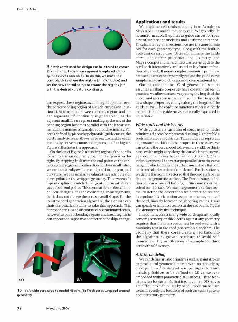
can express these regions as an integral operator overthe corresponding region of a guide curve (see Equa-tion 2). At join points between bending regions and lin-ear segments, G1 continuity is guaranteed, as theadjacent small linear segment making up the end of thebending region becomes parallel with the linear seg-ment as the number of samples approaches infinity. Forcords defined by piecewise polynomial guide curves, thecord’s analytic form allows us to ensure higher-ordercontinuity between connected regions, to G2 or higher.Figure 9 illustrates the approach.

On the left of Figure 9, a bending region of the cord isjoined to a linear segment grown to the sphere on theright. By stepping back from the end points of the con-necting line segment in either direction by a small value,we can analytically evaluate cord position, tangent, andcurvature. We can similarly evaluate these attributes forcurve points on the wrapped geometry. Then we can fita quintic spline to match the tangent and curvature val-ues at both end points. This construction makes a limit-ed local change along the connecting linear segments,but it does not change the cord’s overall shape. For theiterative cord generation algorithm, the step size canlimit the practical ability to take this approach. Thisapproach can also be discontinuous for animated cords,however, as pairs of bending regions and linear segmentscan appear or disappear as contact relationships change.

Applications and resultsWe implemented cords as a plug-in to Autodesk’s

Maya modeling and animation system. We typically usenonuniform cubic B-splines as guide curves for theirease of use in shape modeling and keyframe animation.To calculate ray intersections, we use the appropriateAPI for each geometry type, along with the built-inacceleration structures. Users can animate the guidecurve, appearance properties, and geometry, andMaya’s computational architecture lets us update thecord both interactively and as other keyframe anima-tion plays back. If many complex geometric primitivesare used, users can temporarily reduce the guide curvesample rate to avoid objectionable computational lag.

Our notation in the “Cord generation” sectionassumes all shape properties have constant values. Inpractice, we allow some to vary along the length of thecurve, and users can use a painting interface to specifyhow shape properties change along the length of theguide curve. The cord’s parameterization is directlymapped from the guide curve, as formally expressed inEquation 2.

Wide cords and thick cordsWide cords are a variation of cords used to model

primitives that can be represented as long 2D manifolds,such as flat ribbons or straps. Thick cords can representobjects such as thick tubes or ropes. In these cases, wecan extend the cord model to have more width or thick-ness, which might vary along the curve’s length, as wellas a local orientation that varies along the cord. Orien-tation is expressed as a vector perpendicular to the curvetangent, which defines the surface normal of a flat cordor the radial orientation of a thick cord. For flat surfaces,we define this normal vector so that the cord surface liesflat on the geometric surface. The Frenet frame defini-tion of a curve normal has singularities and is not wellsuited for this task. We use the geometric surface nor-mal to define the orientation for contact points andinterpolate this orientation vector for other segments ofthe cord, linearly between neighboring values. Userscan specify orientation vectors at the endpoints. Figure10a demonstrates this technique.

In addition, constraining wide cords against locallyconvex geometry or thick cords against any geometryrequires that the intersection test be replaced with aproximity test in the cord-generation algorithm. Thegeometry that these cords create is fed back into the algorithm as growth continues to avoid self-intersection. Figure 10b shows an example of a thickcord with self-overlap.

Artistic modelingWe can define artistic primitives such as paint strokes

or procedural geometric curves with an underlyingcurve primitive.1 Existing software packages allow suchartistic primitives to be defined on 2D canvases orembedded within parametric 3D surfaces. These tech-niques can be extremely limiting, as general 3D curvesare difficult to manipulate by hand. Cords can be usedto easily specify the locations of such curves in space orabout arbitrary geometry.

Feature Article

78 May/June 2006

9 Static cords used for design can be altered to ensureG2 continuity. Each linear segment is replaced with aquintic curve (dark blue). To do this, we move thecontrol points where the regions join (light blue) andset the new control points to ensure the regions joinwith the desired curvature continuity.

10 (a) A wide cord used to model ribbon. (b) Thick cords wrapped aroundgeometry.

(a) (b)

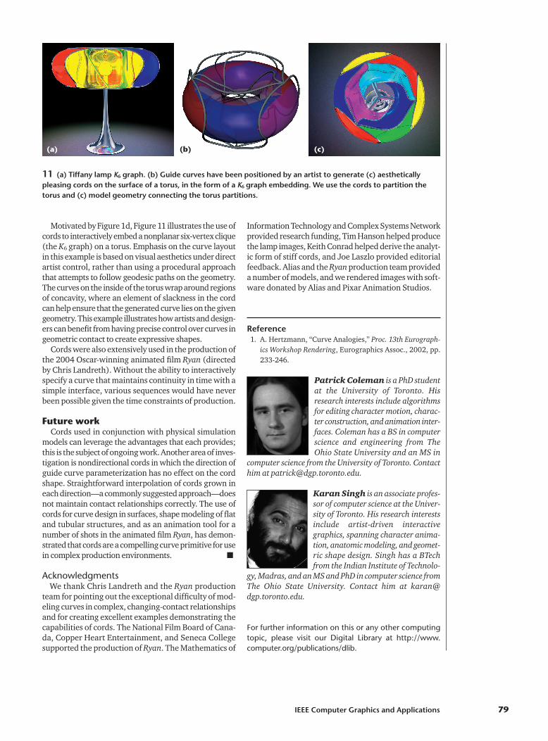
Motivated by Figure 1d, Figure 11 illustrates the use ofcords to interactively embed a nonplanar six-vertex clique(the K6 graph) on a torus. Emphasis on the curve layoutin this example is based on visual aesthetics under directartist control, rather than using a procedural approachthat attempts to follow geodesic paths on the geometry.The curves on the inside of the torus wrap around regionsof concavity, where an element of slackness in the cordcan help ensure that the generated curve lies on the givengeometry. This example illustrates how artists and design-ers can benefit from having precise control over curves ingeometric contact to create expressive shapes.

Cords were also extensively used in the production ofthe 2004 Oscar-winning animated film Ryan (directedby Chris Landreth). Without the ability to interactivelyspecify a curve that maintains continuity in time with asimple interface, various sequences would have neverbeen possible given the time constraints of production.

Future workCords used in conjunction with physical simulation

models can leverage the advantages that each provides;this is the subject of ongoing work. Another area of inves-tigation is nondirectional cords in which the direction ofguide curve parameterization has no effect on the cordshape. Straightforward interpolation of cords grown ineach direction—a commonly suggested approach—doesnot maintain contact relationships correctly. The use ofcords for curve design in surfaces, shape modeling of flatand tubular structures, and as an animation tool for anumber of shots in the animated film Ryan, has demon-strated that cords are a compelling curve primitive for usein complex production environments. ■

AcknowledgmentsWe thank Chris Landreth and the Ryan production

team for pointing out the exceptional difficulty of mod-eling curves in complex, changing-contact relationshipsand for creating excellent examples demonstrating thecapabilities of cords. The National Film Board of Cana-da, Copper Heart Entertainment, and Seneca Collegesupported the production of Ryan. The Mathematics of

Information Technology and Complex Systems Networkprovided research funding, Tim Hanson helped producethe lamp images, Keith Conrad helped derive the analyt-ic form of stiff cords, and Joe Laszlo provided editorialfeedback. Alias and the Ryan production team provideda number of models, and we rendered images with soft-ware donated by Alias and Pixar Animation Studios.

Reference1. A. Hertzmann, “Curve Analogies,” Proc. 13th Eurograph-

ics Workshop Rendering, Eurographics Assoc., 2002, pp.233-246.

Patrick Coleman is a PhD studentat the University of Toronto. Hisresearch interests include algorithmsfor editing character motion, charac-ter construction, and animation inter-faces. Coleman has a BS in computerscience and engineering from TheOhio State University and an MS in

computer science from the University of Toronto. Contacthim at [email protected].

Karan Singh is an associate profes-sor of computer science at the Univer-sity of Toronto. His research interestsinclude artist-driven interactivegraphics, spanning character anima-tion, anatomic modeling, and geomet-ric shape design. Singh has a BTechfrom the Indian Institute of Technolo-

gy, Madras, and an MS and PhD in computer science fromThe Ohio State University. Contact him at [email protected].

For further information on this or any other computingtopic, please visit our Digital Library at http://www.computer.org/publications/dlib.

IEEE Computer Graphics and Applications 79

11 (a) Tiffany lamp K6 graph. (b) Guide curves have been positioned by an artist to generate (c) aestheticallypleasing cords on the surface of a torus, in the form of a K6 graph embedding. We use the cords to partition thetorus and (c) model geometry connecting the torus partitions.

(a) (b) (c)