Copyright (c) Bani Mallic k 1 Lecture 2 Stat 651

Welcome message from author
This document is posted to help you gain knowledge. Please leave a comment to let me know what you think about it! Share it to your friends and learn new things together.
Transcript

Copyright (c) Bani Mallick 1
Lecture 2
Stat 651

Copyright (c) Bani Mallick 2
Topics in Lecture #2 Population and sample parameters
More on populations and samples
The Median and Percentiles
Robustness of the median and IQR, lack of robustness for the mean and standard deviation
Variability: standard deviation and interquartile range (IQR)
Boxplots
Copyright (c) Bani Mallick 3
Book Sections Covered in Lecture #2
Chapter 3.4
Chapter 3.5, up to page 88
Chapter 3.6
Copyright (c) Bani Mallick 4
Review of Lecture #1
We described samples and populations
We want to make inference about populations
We draw samples from the population to do so
Different samples give different results
Copyright (c) Bani Mallick 5
Review of Lecture #1
I will make quite a big deal about the difference between samples and populationsOne major thing we do in statistics is
to quantify: how far is what we see in the sample from what we cannot see in the population?

Copyright (c) Bani Mallick 6
Review of Lecture #1
We defined the relative frequency histogram
This counts the percentage of the sample that falls into computer-generated categories
We studies the NHANES case-control study
This had samples from 2 (sub)populations
Those who developed breast cancer
Those who did not

Copyright (c) Bani Mallick 7
Review of Lecture #1
In the NHANES data, the sample who developed breast cancer seemed to have smaller values of saturated fat than the sample that did not develop breast cancer
What we will try to do today is to quantify those differences
Copyright (c) Bani Mallick 8
Review of Lecture #1: The Population Mean
• In many problems, the goal is to make inference about the population mean of a numerical variable, e.g., saturated fat intake
• The only thing we have available is data from a sample, e.g., the sample mean.
• Define in words what you mean by the population mean and the sample mean!

Copyright (c) Bani Mallick 9
Review of Lecture #1: The Population Mean
• In many problems, the goal is to make inference about the population mean of a numerical variable, e.g., saturated fat intake
• You’re right! The population mean is the average of all the outcomes in the population
• It can’t be measured, hence we take samples.
• BTW, what’s an average?

Copyright (c) Bani Mallick 10
Review of Lecture #1: The Population Mean
Formal definition. If the sample is of size n and the data are X1,…, Xn , then the sample mean is
Total sum of the values in the sample
n
i1 2 n i=1
Σ ΧΧ +Χ +...ΧΧ= =
n n
Number of observations in the sample

Copyright (c) Bani Mallick 11
Parameters and Statistics
Parameter: numerical characteristic of a population
Statistic: numerical characteristic of a sample
PopulationSample

Copyright (c) Bani Mallick 12
Parameters and Statistics
Parameter: numerical characteristic of
a population, called Statistic: numerical characteristic of a
sample, called
PopulationSample

Copyright (c) Bani Mallick 13
Parameters and Statistics
Parameter: numerical characteristic of a
population, called never known!!!)
Statistic: numerical characteristic of a sample, called
PopulationSample
We want to make inference about populationfrom sample
Copyright (c) Bani Mallick 14
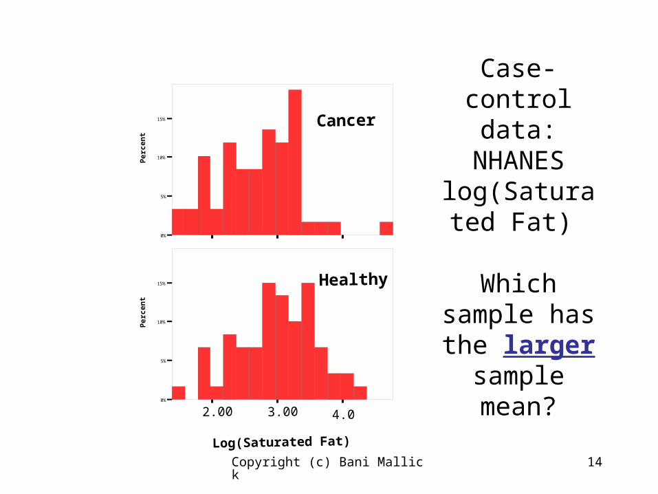
Case-control data: NHANES log(Saturated
Fat)
Which sample has the larger sample mean?
0%
5%
10%
15%
Per
cen
t
Cancer
Healthy
2.00 3.00 4.0
Log(Saturated Fat)
0%
5%
10%
15%
Per
cen
t

Copyright (c) Bani Mallick 15
Case-control data: NHANES log(Saturated
Fat)
Cancer: = 2.70
Healthy: = 2.99
0%
5%
10%
15%
Per
cen
t
Cancer
Healthy
2.00 3.00 4.0
Log(Saturated Fat)
0%
5%
10%
15%
Per
cen
t

Copyright (c) Bani Mallick 16
The Concept of a Median
When we talk about the population median age of graduate students at Texas A&M, what do we mean?
When we talk about the sample median of graduate students at Texas A&M, what do we mean?

Copyright (c) Bani Mallick 17
The Concept of a Median
The population median is the central point
1/2 the population falls below the population median
1/2 the population falls above the population median
Look in newspapers for the use of the median and the mean

Copyright (c) Bani Mallick 18
The Concept of a Median
The sample median is the central point of the sample
1/2 the sample falls below the sample median
1/2 the sample falls above the sample median
We can use the sample median to try to estimate the population median
Remember though, different samples give different numbers
Copyright (c) Bani Mallick 19
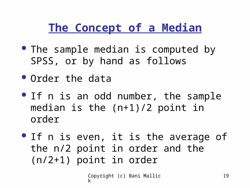
The Concept of a Median
The sample median is computed by SPSS, or by hand as follows
Order the data
If n is an odd number, the sample median is the (n+1)/2 point in order
If n is even, it is the average of the n/2 point in order and the (n/2+1) point in order
Copyright (c) Bani Mallick 20
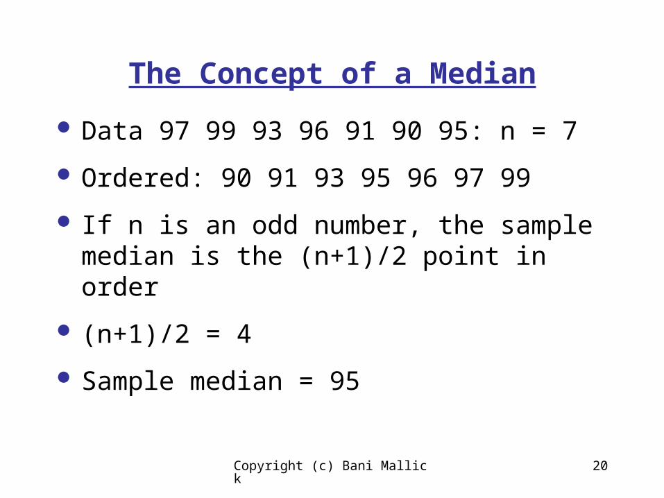
The Concept of a Median
Data 97 99 93 96 91 90 95: n = 7
Ordered: 90 91 93 95 96 97 99
If n is an odd number, the sample median is the (n+1)/2 point in order
(n+1)/2 = 4
Sample median = 95
Copyright (c) Bani Mallick 21
The Concept of a Median
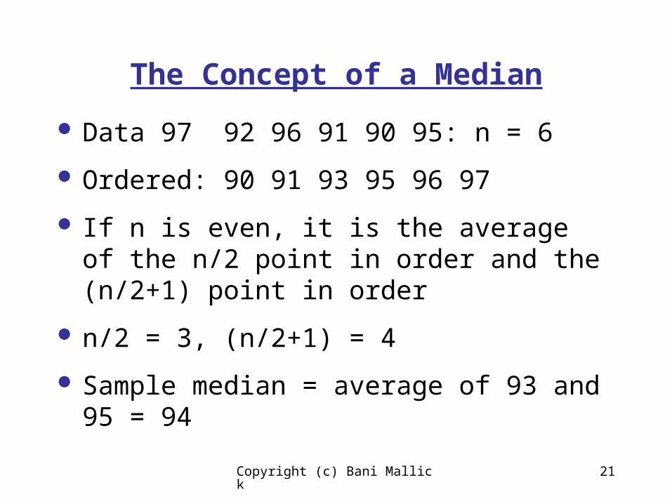
Data 97 92 96 91 90 95: n = 6
Ordered: 90 91 93 95 96 97
If n is even, it is the average of the n/2 point in order and the (n/2+1) point in order
n/2 = 3, (n/2+1) = 4
Sample median = average of 93 and 95 = 94
Copyright (c) Bani Mallick 22
Summary Statistics in SPSS
Select “analyze”, “descriptive statistics”, “explore”
Select your variables (“Dependent”) and you populations (“Factor List”)
Ask for “Statistics”
Cut and paste as needed

Copyright (c) Bani Mallick 23
Descriptives
2.9905 7.969E-02
2.8310
3.1500
3.0015
2.9957
.381
.6173
1.39
4.26
2.88
.9130
-.332 .309
-.138 .608
2.6969 8.362E-02
2.5295
2.8642
2.6886
2.8332
.413
.6423
1.39
4.77
3.38
.8755
.156 .311
.748 .613
Mean
Lower Bound
Upper Bound
95% ConfidenceInterval for Mean
5% Trimmed Mean
Median
Variance
Std. Deviation
Minimum
Maximum
Range
Interquartile Range
Skewness
Kurtosis
Mean
Lower Bound
Upper Bound
95% ConfidenceInterval for Mean
5% Trimmed Mean
Median
Variance
Std. Deviation
Minimum
Maximum
Range
Interquartile Range
Skewness
Kurtosis
Healthy Status Numerical:0 = Healthy, 1 = Cancer
Healthy
Breast Cancer
Log(Saturated Fat)
Statistic Std. Error
SPSS Output for NHANES: you see variable, populations, sample means, medians, minimum and maximum
Copyright (c) Bani Mallick 24
Summary Statistics in SPSS
For both measures of central tendency, healthy women had reported more saturated fat on the day they were interviewed

Copyright (c) Bani Mallick 25
VARIABILITY
Variability is one of the hardest concepts to understand, and to measure.
Variability means how widely spread out the population is
Populations with large variability should have samples that are more spread out than are samples from populations with low variability
Variability is measured by the average distance of points to center
Copyright (c) Bani Mallick 26
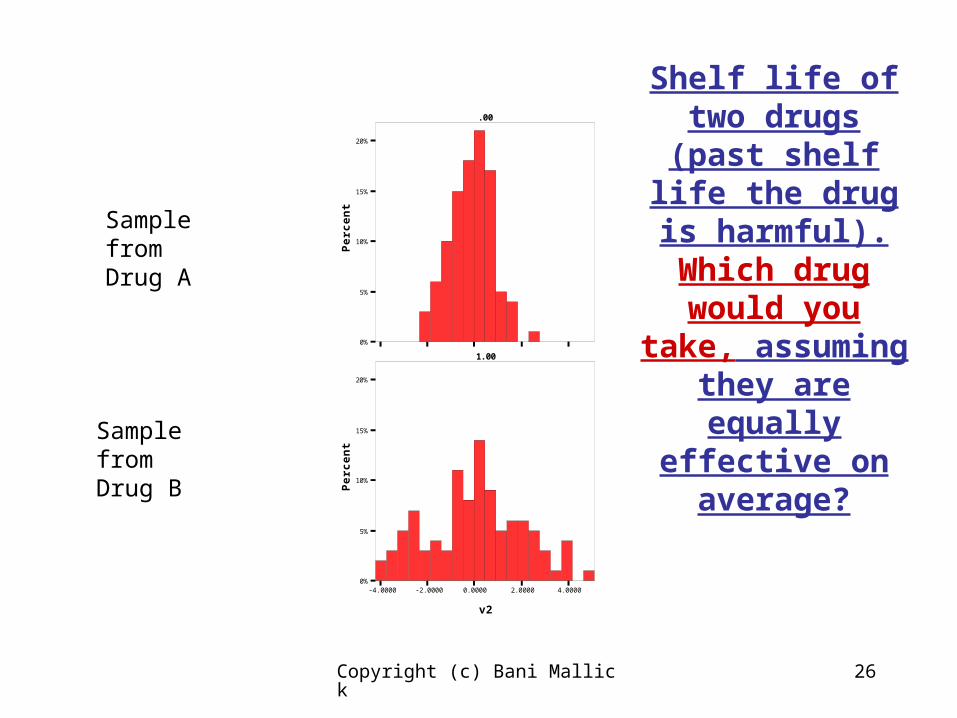
Shelf life of two drugs
(past shelf life the drug is harmful).
Which drug would you
take, assuming they are equally
effective on average?
Sample from Drug A
Sample fromDrug B
0%
5%
10%
15%
20%
Per
cen
t
.00
1.00
-4.0000 -2.0000 0.0000 2.0000 4.0000
v2
0%
5%
10%
15%
20%
Per
cen
t

Copyright (c) Bani Mallick 27
Absolute distance from sample mean
Measuring Variability by Distances
Absolute distance from sample median
iX
i
Squared distance to sample mean
2
i
All numerical measures of variability are measures of “the center of the distance”

Copyright (c) Bani Mallick 28
Variability as average squared distance
The sample variance, s2 is defined as follows
Compute (X - sample mean) for every observation: squared distances
Sum these numbers up
Divide by n-1
Except for the n-1, this is the sample mean of the squared differences

Copyright (c) Bani Mallick 29
COMPUTING FORMULA for the Sample Variance s2
2n
ii 12
X
n 1s
Note how s2 measures how far the data are from the sample mean
Copyright (c) Bani Mallick 30
The Standard Devation, s
The sample standard deviation is called s
It is the square root of the sample variance
Its units are the same as the units of the data
2s s
Copyright (c) Bani Mallick 31
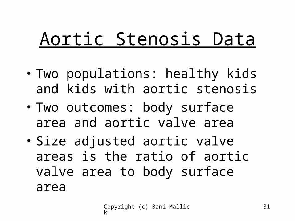
Aortic Stenosis Data
• Two populations: healthy kids and kids with aortic stenosis
• Two outcomes: body surface area and aortic valve area
• Size adjusted aortic valve areas is the ratio of aortic valve area to body surface area

Copyright (c) Bani Mallick 32
Aortic Valve Area for
Healthy and Stenotic Kids
Which has larger mean,
larger variance?
5%
10%
15%
20%
25%
Per
cen
t
Healthy
Stenotic
0.000 1.000 2.000 3.000
Aortic Valve Area
5%
10%
15%
20%
25%
Per
cen
t

Copyright (c) Bani Mallick 33
Aortic Valve Area for
Healthy and Stenotic Kids
Which has larger mean,
larger variance?
5%
10%
15%
20%
25%
Per
cen
t
Healthy
Stenotic
0.000 1.000 2.000 3.000
Aortic Valve Area
5%
10%
15%
20%
25%
Per
cen
t
Mean = 1.06Median = 0.80std dev = 0.78
Mean = 0.83Median = 0.69std dev = 0.64
Copyright (c) Bani Mallick 34
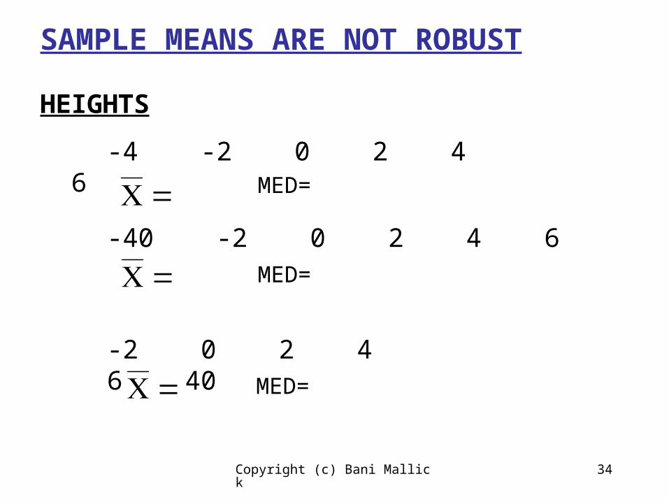
SAMPLE MEANS ARE NOT ROBUST
HEIGHTS
-4 -2 0 2 4 6
MED=
-40 -2 0 2 4 6
MED=
-2 0 2 4 6 40
MED=
Copyright (c) Bani Mallick 35
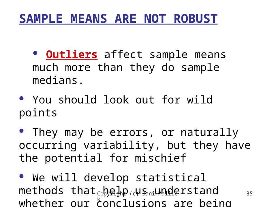
SAMPLE MEANS ARE NOT ROBUST
Outliers affect sample means much more than they do sample medians.
You should look out for wild points
They may be errors, or naturally occurring variability, but they have the potential for mischief
We will develop statistical methods that help us understand whether our conclusions are being driven by a few wild points.
Copyright (c) Bani Mallick 36
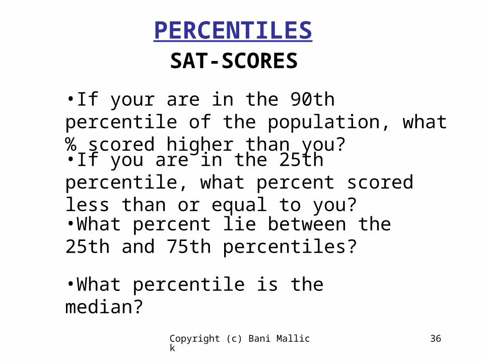
PERCENTILESSAT-
SCORES•If your are in the 90th percentile of the population, what % scored higher than you?•If you are in the 25th percentile, what percent scored less than or equal to you?
•What percent lie between the 25th and 75th percentiles?
•What percentile is the median?
Copyright (c) Bani Mallick 37
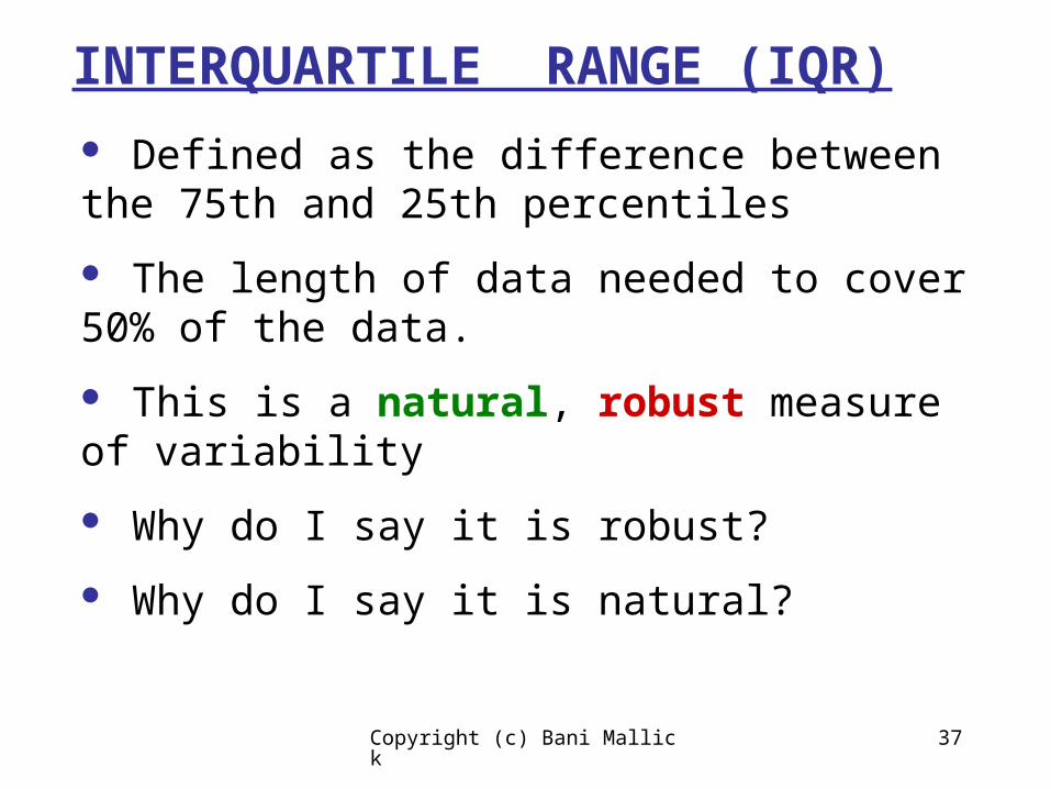
INTERQUARTILE RANGE (IQR) Defined as the difference between the 75th and 25th percentiles
The length of data needed to cover 50% of the data.
This is a natural, robust measure of variability
Why do I say it is robust?
Why do I say it is natural?

Copyright (c) Bani Mallick 38
Aortic Valve Area for
Healthy and Stenotic Kids
Which has larger mean,
larger variance?
5%
10%
15%
20%
25%
Per
cen
t
Healthy
Stenotic
0.000 1.000 2.000 3.000
Aortic Valve Area
5%
10%
15%
20%
25%
Per
cen
t
Mean = 1.06Median = 0.80std dev = 0.78IQR = 0.98
Mean = 0.83Median = 0.69std dev = 0.64IQR = 0.59

Copyright (c) Bani Mallick 39
INTERQUARTILE RANGE Defined as the difference between the
75th and 25th percentiles
The length of data needed to cover 50% of the data.
This is a natural, robust measure of variability
If comparisons of variability are different for the standard deviation and the IQR, good chance of an outlier

Copyright (c) Bani Mallick 40
Descriptives
2.9905 7.969E-02
2.8310
3.1500
3.0015
2.9957
.381
.6173
1.39
4.26
2.88
.9130
-.332 .309
-.138 .608
2.6969 8.362E-02
2.5295
2.8642
2.6886
2.8332
.413
.6423
1.39
4.77
3.38
.8755
.156 .311
.748 .613
Mean
Lower Bound
Upper Bound
95% ConfidenceInterval for Mean
5% Trimmed Mean
Median
Variance
Std. Deviation
Minimum
Maximum
Range
Interquartile Range
Skewness
Kurtosis
Mean
Lower Bound
Upper Bound
95% ConfidenceInterval for Mean
5% Trimmed Mean
Median
Variance
Std. Deviation
Minimum
Maximum
Range
Interquartile Range
Skewness
Kurtosis
Healthy Status Numerical:0 = Healthy, 1 = CancerHealthy
Breast Cancer
Look for variance, standard deviation and IQR
Log(Saturated Fat)Statistic Std. Error

Copyright (c) Bani Mallick 41
Box Plots
Box plots are a means of visualizing data from different populations, especially comparing them
Far less clunky than histograms
Clear definitions, don’t have to worry about # of bars, class intervals, etc.
Easily available

Copyright (c) Bani Mallick 42
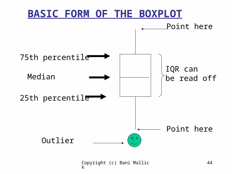
BASIC FORM OF THE BOXPLOT
75th percentile
Median
25th percentile
IQR canbe read off

Copyright (c) Bani Mallick 43
Box Plot Additions: Technical
To the basic box, whiskers are added:
Go out to furthest point 1.5 IQR from 75th and 25th percentiles
• Any other points are called “Suspicious” “Extreme” “Outliers”
Copyright (c) Bani Mallick 44
BASIC FORM OF THE BOXPLOT
75th percentile
Median
25th percentile
IQR canbe read off
Point here
Point here
Outlier

Copyright (c) Bani Mallick 45
IQR AS A MEASURE OF VARIABILITY
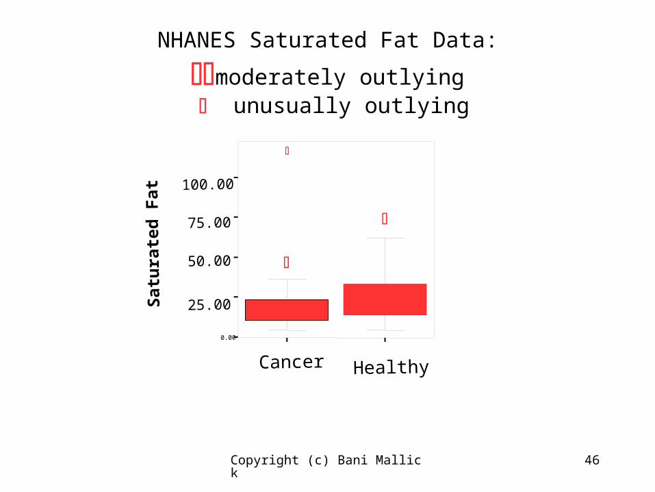
The box is from 25th to 75th sample percentileThis means 50% of the data are in the boxHence, IQR= range needed to cover 50% of the data IQR is a very robust measure of variability which can be judged graphically
Copyright (c) Bani Mallick 46
NHANES Saturated Fat Data:
moderately outlying unusually outlying
Cancer Healthy
0.00
25.00
50.00
75.00
100.00
Sat
ura
ted
Fat

Copyright (c) Bani Mallick 47
Box Plots
The SPSS plot actually displays the median line, but it did not translate into powerpoint
You go to graphs, interactive and boxplot to get these things
Here’s about what the thing looks like in SPSS (then I’ll show you SPSS)
Copyright (c) Bani Mallick 48
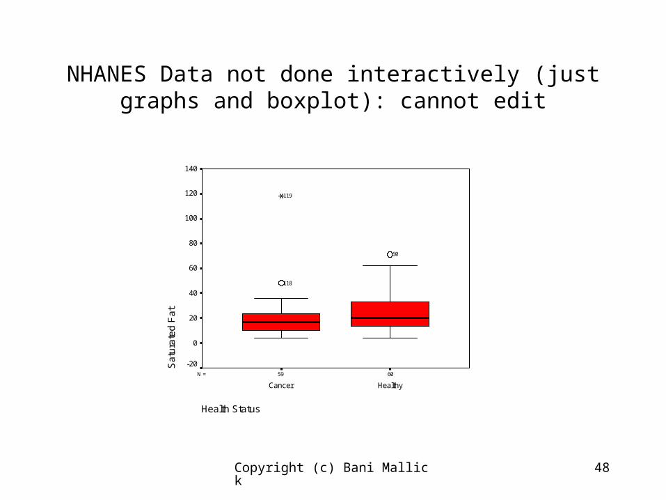
NHANES Data not done interactively (just graphs and boxplot): cannot edit
6059N =
Health Status
HealthyCancer
Sa
tura
ted
Fa
t140
120
100
80
60
40
20
0
-20
60
118
119
Copyright (c) Bani Mallick 49
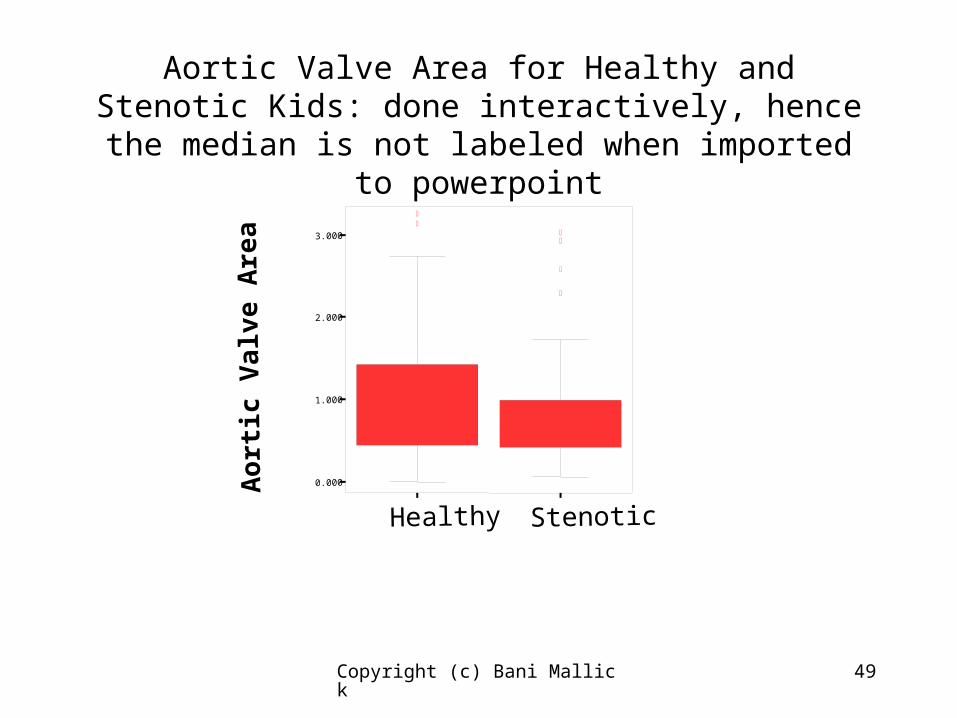
Aortic Valve Area for Healthy and Stenotic Kids: done interactively, hence the median is not
labeled when imported to powerpoint
Healthy Stenotic
0.000
1.000
2.000
3.000
Ao
rtic
Va
lve
Are
a
Related Documents