Copyright by Smriti Rajan Ramakrishnan 2010 - CiteSeerX

Copyright

by

Smriti Rajan Ramakrishnan

2010

The Dissertation Committee for Smriti Rajan Ramakrishnancertifies that this is the approved version of the following dissertation:

A Systems Approach to Computational Protein

Identification

Committee:

Daniel P Miranker, Supervisor

Inderjit Dhillon

Edward M Marcotte

Raymond J Mooney

William H Press


Identification

by

Smriti Rajan Ramakrishnan, B.E., M.S.

DISSERTATION

Presented to the Faculty of the Graduate School of

The University of Texas at Austin

in Partial Fulfillment

of the Requirements

for the Degree of

DOCTOR OF PHILOSOPHY

THE UNIVERSITY OF TEXAS AT AUSTIN

May 2010

Dedicated to Paty

Acknowledgments

Being grateful to so many who have influenced my grad-school years, I hereby

renege on all promises to self that the Acknowledgements section wouldn’t ramble.

Many thanks to my adviser Professor Miranker, and to Professors Marcotte,

Dhillon, Mooney and Press for agreeing to be on my dissertation committee. I learnt

a great many things about research, science, engineering, writing, and presentation

from my PhD adviser, Professor Dan Miranker. My work has largely benefited from

his understanding of the challenges in collaborative interdisciplinary research. Above

all, I am grateful for his guidance in shaping me into an independent researcher.

I am privileged to have worked closely with Professor Edward Marcotte -

his enthusiasm for science is contagious. His wide knowledge of biology and com-

putational science provided the perfect guidance as I transitioned from engineering

to interdisciplinary science. I have always appreciated his attention to detail while

giving feedback on my work and manuscripts.

Professor Inderjit Dhillon’s classes were my formal introduction to data min-

ing. I am grateful for his feedback on the network-assisted approaches in this disser-

tation. Professor Raymond Mooney’s machine learning class clinched my decision

to work towards a PhD. His rigorous approach to experimental methodology has

largely shaped my way of addressing the experimental evaluation issues that are

central to bioinformatics. I remain in awe of Professor William Press’ breadth of

experience, depth of knowledge, and his total accessibility to students. I feel very

privileged to have had his feedback on my work, and I hope to have imbibed his

v

teachings in computational statistics and, more generally, in conducting high-quality

scientific research.

I am truly grateful to Dr. Margaret Myers for discussions on statistics and

everything associated, to Professor Kathryn McKinley for her encouragement when

applying to the PhD program, and Dr. Dipti Deodhare at CAIR, Bangalore for

introducing me to research.

To the Miranker lab: Rui Mao and Weijia Xu who have been great mentors,

Willard Willard for being an essential part of MSFound, Hamid Tirmizi for being

a supremely organized class project partner, and to Lee Parnell, Juan Sequeda and

Ferner Cilloniz for being a high-energy research group.

To the Marcotte lab: John Prince and Aleksey Nakorchevskiy were my first

mass spec guides, Christine Vogel who has watched over me (and the mass spec)

since and is Tenacity personified, Taejoon Kwon, Rong Wang, Zhihua Li and Dan

Boutz for data and for learning, and Martin Blom and Peggy Wang for discussions

on the joys of gene network analysis.

To Laurie Alvarez, Alisha Hall, Lydia Griffith, Gloria Ramirez and Katherine

Utz for all things administrative, and to the University of Texas libraries for feeding

my internal bookworm.

To Sowmya Ramachandran, for being my closest friend and strongest support

in Austin, Suriya Subramanian for being my tech advice and my cribbing shoulder,

and Upendra Shevade for being a true comrade and supplying my daily shot of

laughter. To Meenakshi Venkataraman, Geethapriya Raghavan, Karthik Raghavan

and Sean Leather for camaraderie in early grad school years, and to the LJ bunch

for simply listening - you know who you are.

vi

To my oldest friends: Shubha Pai, Vidya Selvavinayakam, Srividya Mohan,

Milin Mary George, Nutan Raj and Rajeev Rao for always being a phone-call away.

To my distributed family for giving me homes across three continents (and al-

ways asking when I was going to graduate), to my in-laws, Mr. and Mrs. Srinivasan,

for their support, patience and unquestioning faith, and to Santhosh Srinivasan and

Shalini Kalia for my second home in California.

To my husband, Vishwas Srinivasan, for being my foil and my anchor, for

putting up with all the drama, and for having enough faith for both of us.

My parents have been my single biggest source of strength, my enablers, and

my loudest cheering squad. I consider it the highest privilege to have been able

to pursue education and research with no real-world worries to speak of - without

them, literally and figuratively, none of this would exist.

vii


Identification

Publication No.

Smriti Rajan Ramakrishnan, Ph.D.

The University of Texas at Austin, 2010

Supervisor: Daniel P Miranker

Proteomics is the science of understanding the dynamic protein content of

an organism’s cells (its proteome), which is one of the largest current challenges in

biology. Computational proteomics is an active research area that involves in-silico

methods for the analysis of high-throughput protein identification data. Current

methods are based on a technology called tandem mass spectrometry (MS/MS)

and suffer from low coverage and accuracy, reliably identifying only 20-40% of the

proteome. This dissertation addresses recall, precision, speed and scalability of

computational proteomics experiments.

This research goes beyond the traditional paradigm of analyzing MS/MS

experiments in isolation, instead learning priors of protein presence from the joint

analysis of various systems biology data sources. This integrative ‘systems’ approach

to protein identification is very effective, as demonstrated by two new methods.

The first, MSNet, introduces a social model for protein identification and leverages

functional dependencies from genome-scale, probabilistic, gene functional networks.

The second, MSPresso, learns a gene expression prior from a joint analysis of mRNA

and proteomics experiments on similar samples.

viii

These two sources of prior information result in more accurate estimates of

protein presence, and increase protein recall by as much as 30% in complex samples,

while also increasing precision. A comprehensive suite of benchmarking datasets is

introduced for evaluation in yeast. Methods to assess statistical signicance in the

absence of ground truth are also introduced and employed whenever applicable.

This dissertation also describes a database indexing solution to improve speed

and scalability of protein identification experiments. The method, MSFound, cus-

tomizes a metric-space database index and its associated approximate k-nearest-

neighbor search algorithm with a semi-metric distance designed to match noisy

spectra. MSFound achieves an order of magnitude speedup over traditional spectra

database searches while maintaining scalability.

ix

Table of Contents

Acknowledgments v

Abstract viii

List of Tables xv

List of Figures xvi

Chapter 1. Introduction 1

1.1 Motivation . . . . . . . . . . . . . . . . . . . . . . . . . . . . . . . . . 1

1.1.1 Research philosophy . . . . . . . . . . . . . . . . . . . . . . . . 2

1.2 Roadblocks to computational protein identification . . . . . . . . . . . 3

1.3 Research goals and contributions . . . . . . . . . . . . . . . . . . . . . 4

1.3.1 Improving coverage and accuracy via integrative analysis . . . . 4

1.3.1.1 Using gene networks . . . . . . . . . . . . . . . . . . . 5

1.3.1.2 Using gene expression experiments . . . . . . . . . . . 6

1.3.1.3 Benchmarking sets for protein identification in com-plex samples . . . . . . . . . . . . . . . . . . . . . . . . 6

1.3.2 Improving speed and scalability by database indexing . . . . . 7

1.4 Chapter overview . . . . . . . . . . . . . . . . . . . . . . . . . . . . . 8

Chapter 2. Background 9

2.1 MS and MS/MS . . . . . . . . . . . . . . . . . . . . . . . . . . . . . . 9

2.1.1 Mass spectrometry biases . . . . . . . . . . . . . . . . . . . . . 12

2.2 Mass spectrometry via database search . . . . . . . . . . . . . . . . . 12

2.2.1 Uncertainty in database lookup . . . . . . . . . . . . . . . . . . 13

2.3 Stages of computational protein identification . . . . . . . . . . . . . . 15

2.3.1 Spectra matching . . . . . . . . . . . . . . . . . . . . . . . . . 15

2.3.2 Peptide identification . . . . . . . . . . . . . . . . . . . . . . . 16

2.3.3 Protein identification . . . . . . . . . . . . . . . . . . . . . . . 17

2.4 Experimental evaluation of MS/MS experiments . . . . . . . . . . . . 19

x

2.4.1 Control mixtures and shuffled databases . . . . . . . . . . . . . 19

2.4.1.1 Concatenated vs. separate decoy database . . . . . . . 20

2.5 Evaluation metrics and terminology . . . . . . . . . . . . . . . . . . . 21

2.5.1 Literature-based ground truth . . . . . . . . . . . . . . . . . . 23

2.5.2 Error estimation without ground-truth . . . . . . . . . . . . . . 24

2.5.3 False Discovery Rates in genomic and proteomic literature . . . 24

Chapter 3. Datasets and benchmarking 26

3.1 Protein and mRNA datasets . . . . . . . . . . . . . . . . . . . . . . . 26

3.1.1 Yeast . . . . . . . . . . . . . . . . . . . . . . . . . . . . . . . . 26

3.1.1.1 Yeast grown in rich medium . . . . . . . . . . . . . . . 27

3.1.1.2 Yeast grown in rich medium, polysomal fraction . . . . 27

3.1.1.3 Yeast grown in minimal medium . . . . . . . . . . . . 27

3.1.2 E. coli . . . . . . . . . . . . . . . . . . . . . . . . . . . . . . . . 27

3.1.3 Human . . . . . . . . . . . . . . . . . . . . . . . . . . . . . . . 28

3.1.3.1 DAOY medulloblastoma cell line . . . . . . . . . . . . 28

3.1.3.2 HEK293T kidney cells . . . . . . . . . . . . . . . . . . 28

3.2 Benchmarking . . . . . . . . . . . . . . . . . . . . . . . . . . . . . . . 28

3.2.1 Literature-based reference sets . . . . . . . . . . . . . . . . . . 29

3.2.1.1 Constructing a benchmark set . . . . . . . . . . . . . . 30

3.3 Availability . . . . . . . . . . . . . . . . . . . . . . . . . . . . . . . . 31

Chapter 4. Integrative analysis of gene expression and proteomicsexperiments 35

4.1 Introduction . . . . . . . . . . . . . . . . . . . . . . . . . . . . . . . . 35

4.2 Methods . . . . . . . . . . . . . . . . . . . . . . . . . . . . . . . . . . 36

4.2.1 Estimating conditional probabilities . . . . . . . . . . . . . . . 37

4.3 Results . . . . . . . . . . . . . . . . . . . . . . . . . . . . . . . . . . . 41

4.3.1 Yeast . . . . . . . . . . . . . . . . . . . . . . . . . . . . . . . . 43

4.3.1.1 Yeast grown in rich medium . . . . . . . . . . . . . . . 43

4.3.1.2 Other yeast data . . . . . . . . . . . . . . . . . . . . . 46

4.3.2 E. coli sample . . . . . . . . . . . . . . . . . . . . . . . . . . . 48

4.3.3 Human sample . . . . . . . . . . . . . . . . . . . . . . . . . . . 48

4.4 Applicability in the absence of literature-curated ground-truth . . . . 49

4.4.1 Reusing pre-trained models . . . . . . . . . . . . . . . . . . . . 51

xi

4.4.2 Evaluation using decoy proteins and random P (K|M) . . . . . 51

4.5 Discussion . . . . . . . . . . . . . . . . . . . . . . . . . . . . . . . . . 54

4.5.1 KD-trees for density estimation . . . . . . . . . . . . . . . . . . 54

4.5.2 Biological implications . . . . . . . . . . . . . . . . . . . . . . . 58

4.5.2.1 The relationship between mRNA abundance and pro-tein presence . . . . . . . . . . . . . . . . . . . . . . . 58

4.5.2.2 Estimating the size of the expressed yeast proteome . . 58

4.5.2.3 Correlation between mRNA and probability of proteinpresence . . . . . . . . . . . . . . . . . . . . . . . . . . 59

4.5.3 Demoted proteins . . . . . . . . . . . . . . . . . . . . . . . . . 60

4.5.4 Reliability of MS/MS protein probabilities . . . . . . . . . . . . 61

4.6 Related Work . . . . . . . . . . . . . . . . . . . . . . . . . . . . . . . 61

4.6.1 Protein abundance vs. mRNA abundance . . . . . . . . . . . . 63

4.7 Software and availability . . . . . . . . . . . . . . . . . . . . . . . . . 64

Chapter 5. Network priors from gene functional networks 65

5.1 Introduction . . . . . . . . . . . . . . . . . . . . . . . . . . . . . . . . 65

5.2 Methods . . . . . . . . . . . . . . . . . . . . . . . . . . . . . . . . . . 67

5.2.1 MSNet algorithm . . . . . . . . . . . . . . . . . . . . . . . . . . 67

5.2.2 Convergence . . . . . . . . . . . . . . . . . . . . . . . . . . . . 70

5.2.3 Relationship of MSNet to Google’s PageRank . . . . . . . . . . 71

5.2.3.1 PageRank . . . . . . . . . . . . . . . . . . . . . . . . . 71

5.2.3.2 Topic-sensitive or Personalized PageRank . . . . . . . . 73

5.2.3.3 Relationship . . . . . . . . . . . . . . . . . . . . . . . . 74

5.3 Datasets . . . . . . . . . . . . . . . . . . . . . . . . . . . . . . . . . . 76

5.4 Evaluation Methodology . . . . . . . . . . . . . . . . . . . . . . . . . 77

5.4.1 Evaluation against a protein reference set . . . . . . . . . . . . 78

5.4.2 Evaluation independent of a protein reference set . . . . . . . . 78

5.5 Results . . . . . . . . . . . . . . . . . . . . . . . . . . . . . . . . . . . 79

5.5.1 Yeast grown in rich medium . . . . . . . . . . . . . . . . . . . . 80

5.5.2 Yeast grown in minimal medium . . . . . . . . . . . . . . . . . 82

5.5.3 Yeast polysomal fraction . . . . . . . . . . . . . . . . . . . . . 83

5.5.4 Human samples . . . . . . . . . . . . . . . . . . . . . . . . . . 84

5.5.5 Performance on different MS/MS pipelines . . . . . . . . . . . 84

5.6 Discussion . . . . . . . . . . . . . . . . . . . . . . . . . . . . . . . . . 86

xii

5.6.1 Demoted proteins . . . . . . . . . . . . . . . . . . . . . . . . . 86

5.6.2 Gene to protein mapping . . . . . . . . . . . . . . . . . . . . . 86

5.7 Related work . . . . . . . . . . . . . . . . . . . . . . . . . . . . . . . . 87

5.8 Availability . . . . . . . . . . . . . . . . . . . . . . . . . . . . . . . . 90

Chapter 6. Network priors: graphical models and Markov RandomFields 101

6.1 Markov Random Fields . . . . . . . . . . . . . . . . . . . . . . . . . . 102

6.2 Message-passing inference for graphical models . . . . . . . . . . . . . 103

6.2.1 Sum-product algorithm (belief propagation) . . . . . . . . . . . 106

6.2.2 Max-product algorithm (belief revision) . . . . . . . . . . . . . 107

6.3 An MRF model on gene networks . . . . . . . . . . . . . . . . . . . . 108

6.3.1 Model definition . . . . . . . . . . . . . . . . . . . . . . . . . . 108

6.3.2 Including a gene expression prior (mRNA) . . . . . . . . . . . . 109

6.4 Gaussian field label propagation . . . . . . . . . . . . . . . . . . . . . 110

6.5 Results . . . . . . . . . . . . . . . . . . . . . . . . . . . . . . . . . . . 111

6.5.1 Evaluation Methodology . . . . . . . . . . . . . . . . . . . . . . 111

6.5.2 Evaluation . . . . . . . . . . . . . . . . . . . . . . . . . . . . . 112

6.5.3 Comparison to MSNet and MSPresso . . . . . . . . . . . . . . 115

6.5.4 Discussion . . . . . . . . . . . . . . . . . . . . . . . . . . . . . 115

6.6 MSNet in a Markov Random Field framework . . . . . . . . . . . . . 116

6.6.1 Model definition . . . . . . . . . . . . . . . . . . . . . . . . . . 116

6.6.2 Mapping . . . . . . . . . . . . . . . . . . . . . . . . . . . . . . 117

Chapter 7. MSFound: database indexing for peptide spectra identi-fication 119

7.1 Introduction . . . . . . . . . . . . . . . . . . . . . . . . . . . . . . . . 119

7.2 Methods . . . . . . . . . . . . . . . . . . . . . . . . . . . . . . . . . . 121

7.2.1 Metric space indexing for database search . . . . . . . . . . . . 121

7.2.2 MoBIoS’ k-NN search algorithm . . . . . . . . . . . . . . . . . 123

7.2.3 Internal data representation . . . . . . . . . . . . . . . . . . . . 124

7.2.4 Distance metrics . . . . . . . . . . . . . . . . . . . . . . . . . . 125

7.2.5 Modifying MVP trees for semi-metric distances . . . . . . . . . 128

7.3 Datasets . . . . . . . . . . . . . . . . . . . . . . . . . . . . . . . . . . 129

7.3.1 Test databases . . . . . . . . . . . . . . . . . . . . . . . . . . . 129

7.3.2 Test sets and ground-truth . . . . . . . . . . . . . . . . . . . . 130

xiii

7.4 Parameter Selection . . . . . . . . . . . . . . . . . . . . . . . . . . . . 131

7.5 Results . . . . . . . . . . . . . . . . . . . . . . . . . . . . . . . . . . . 132

7.5.1 Index performance and comparison of distance functions . . . . 132

7.5.2 Scalability . . . . . . . . . . . . . . . . . . . . . . . . . . . . . 133

7.5.3 Intrinsic dimensionality as an indicator of search performance . 137

7.6 Fine filtering . . . . . . . . . . . . . . . . . . . . . . . . . . . . . . . . 139

7.6.1 Results . . . . . . . . . . . . . . . . . . . . . . . . . . . . . . . 141

7.7 Discussion . . . . . . . . . . . . . . . . . . . . . . . . . . . . . . . . . 142

7.7.1 Other distance metrics: Hamming Distance . . . . . . . . . . . 142

7.7.2 Charge state . . . . . . . . . . . . . . . . . . . . . . . . . . . . 143

7.8 Related work . . . . . . . . . . . . . . . . . . . . . . . . . . . . . . . . 144

7.8.1 Hash-based indexing . . . . . . . . . . . . . . . . . . . . . . . . 144

7.8.2 Clustering experimental spectra to achieve speedup . . . . . . . 145

7.8.3 Detecting post-translational modifications . . . . . . . . . . . . 146

Chapter 8. Conclusions and Future Directions 148

8.1 Contributions . . . . . . . . . . . . . . . . . . . . . . . . . . . . . . . 148

8.1.1 A systemic, integrative approach to computational proteomics . 149

8.1.2 Database indexing framework for peptide spectrum matching . 150

8.1.3 Benchmarking and evaluation . . . . . . . . . . . . . . . . . . . 150

8.2 Future directions . . . . . . . . . . . . . . . . . . . . . . . . . . . . . 151

8.2.1 Integrative analysis with biological pathways . . . . . . . . . . 151

8.2.2 Integrative, quantitative proteomics . . . . . . . . . . . . . . . 152

8.2.3 Knowledge-based detection of post-translationally modified pep-tides . . . . . . . . . . . . . . . . . . . . . . . . . . . . . . . . . 153

8.2.4 Consensus across multiple high-throughput proteomics experi-ments . . . . . . . . . . . . . . . . . . . . . . . . . . . . . . . . 154

Bibliography 156

Vita 171

xiv

List of Tables

2.1 Background: Experimental evaluation measures and terminology . . . 22

3.1 Datasets: Mass spectrometry data . . . . . . . . . . . . . . . . . . . . 33

3.2 Datasets: mRNA data . . . . . . . . . . . . . . . . . . . . . . . . . . 34

3.3 Datasets: Protein reference sets . . . . . . . . . . . . . . . . . . . . . 34

4.1 MSPresso: Performance evaluation of ‘self’ models . . . . . . . . . . . 43

4.2 MSPresso: Performance evaluation of ‘reuse’ models . . . . . . . . . . 52

4.3 MSPresso: Performance evaluation without a reference set . . . . . . 55

5.1 MSNet: Performance evaluation . . . . . . . . . . . . . . . . . . . . . 90

5.2 MSNet: Performance evaluation without MS/MS evidence . . . . . . 90

5.3 MSNet: Performance evaluation without a protein reference set . . . 91

5.4 MSNet: Performance evaluation across MS/MS software pipelines . . 92

6.1 Comparison of MSPresso, MSNet and MRF models . . . . . . . . . . 115

7.1 MSFound: Test databases . . . . . . . . . . . . . . . . . . . . . . . . 130

xv

List of Figures

2.1 Background: Typical bottom-up MS/MS proteomics experiment andanalysis . . . . . . . . . . . . . . . . . . . . . . . . . . . . . . . . . . 11

3.1 Clustering reference experiments to construct a protein identificationground-truth . . . . . . . . . . . . . . . . . . . . . . . . . . . . . . . 32

4.1 MSPresso: Introduction . . . . . . . . . . . . . . . . . . . . . . . . . 38

4.2 MSPresso: Estimating P (K|M) for yeast . . . . . . . . . . . . . . . . 39

4.3 MSPresso: Estimating P(K) from protein reference sets . . . . . . . . 40

4.4 MSPresso: Estimating P (K|M) for other organisms . . . . . . . . . . 42

4.5 MSPresso: Results on yeast grown in rich medium . . . . . . . . . . . 45

4.6 MSPresso: Validation of identified proteins . . . . . . . . . . . . . . . 46

4.7 MSPresso: Results on other yeast data . . . . . . . . . . . . . . . . . 47

4.8 MSPresso: Results on E. coli and human data . . . . . . . . . . . . . 50

4.9 MSPresso: Estimating probabilities without a protein reference set . . 53

4.10 MSPresso: KD-tree space partitioning . . . . . . . . . . . . . . . . . 57

4.11 MSPresso: Protein probability vs. mRNA abundance . . . . . . . . . 59

4.12 MSPresso: Protein probability vs. protein abundance . . . . . . . . . 60

4.13 MSPresso: Are protein probabilities true probabilities? . . . . . . . . 62

5.1 MSNet: Feasibility Analysis . . . . . . . . . . . . . . . . . . . . . . . 66

5.2 MSNet: Sensitivity of ROC to parameters . . . . . . . . . . . . . . . 70

5.3 MSNet: Validation of MSNet identifications . . . . . . . . . . . . . . 93

5.4 MSNet: Results on yeast grown in rich medium . . . . . . . . . . . . 93

5.5 MSNet: Rescued proteins and their network neighbors . . . . . . . . 94

5.6 MSNet: Results on other yeast data . . . . . . . . . . . . . . . . . . . 95

5.7 MSNet: Results using different MS/MS software pipelines . . . . . . 96

5.8 MSNet: Sensitivity of FDRshuff to parameters . . . . . . . . . . . . . 97

5.9 MSNet: Parameter estimation . . . . . . . . . . . . . . . . . . . . . . 98

5.10 MSNet: Performance of PageRank . . . . . . . . . . . . . . . . . . . 99

5.11 MSNet: Null and true score distributions . . . . . . . . . . . . . . . . 100

xvi

6.1 Incorporating mRNA abundance data into the MRF model . . . . . . 110

6.2 MRF parameter estimation . . . . . . . . . . . . . . . . . . . . . . . 113

6.3 Performance evaluation of MRF models . . . . . . . . . . . . . . . . . 114

7.1 MSFound: Parameter estimation for precursor mass tolerance . . . . 131

7.2 MSFound: Parameter estimation for search . . . . . . . . . . . . . . . 131

7.3 MSFound: Results for range and k-NN searches . . . . . . . . . . . . 133

7.4 MSFound: Tandem cosine distance vs. fuzzy cosine distance . . . . . 134

7.5 MSFound: Tandem cosine distance vs. precursor mass filter . . . . . 134

7.6 MSFound: Scalability . . . . . . . . . . . . . . . . . . . . . . . . . . . 135

7.7 MSFound: Estimating intrinsic dimensionality . . . . . . . . . . . . . 138

7.8 MSFound: Evaluating Hamming distance . . . . . . . . . . . . . . . . 143

8.1 Screen-shot of proteomics-pathways tool . . . . . . . . . . . . . . . . 152

xvii

Chapter 1

Introduction

1.1 Motivation

Proteomics is the study of all proteins in a cell or tissue. The protein content

of a cell changes constantly based on cellular condition, unlike its relatively static

DNA. The term shotgun proteomics refers to the high-throughput identification of

proteins via tandem mass spectrometry (MS/MS) technology. The name is a hat-tip

to the rapid shotgun DNA sequencing technology that fueled the genomic revolution

and led to the sequencing of the human genome. Computational proteomics is

an active research area that involves in-silico methods for the analysis of high-

throughput mass spectrometry data.

Characterizing a cell’s protein content is relevant to the entire spectrum of

biotechnology goals, including disease diagnosis, drug development and bioengineer-

ing. For instance, comparative proteomics analysis of diseased and normal cells has

the potential to lead to the identification of biomarkers1 that can be used in the

early detection of cancer [117].

Tandem mass spectrometry (MS/MS) is the mainstream high-throughput

technology for measuring protein expression in complex samples2. MS/MS methods

have the potential of detecting thousands of proteins in a high-throughput manner.

1biomarker: genetic material differentially expressed in diseased cells2A complex sample can contain thousands of proteins. Protein expression refers to the presence

and/or amount of protein in a cell

1

Using particle acceleration through electric fields, mass spectrometry revolutionized

proteomics by moving the focus from analysis of gel-images to analysis of real-

valued, mass-to-charge measurements. Traditional methods like two-dimensional

gel electrophoresis are far more time-consuming and labor-intensive.

However, the high-throughput MS/MS blessing brought with it a slew of

data analysis challenges and lower than expected sensitivity and sample coverage.

Though a few thousand proteins can be detected using highly sensitive and expensive

mass spectrometers [138], in most situations only 20-40% of expected proteins are

currently confidently identified by statistical analysis of MS/MS data. As a result,

proteomics has not yet reached its promised potential in biomarker discovery [113].

1.1.1 Research philosophy

MS/MS experiments are currently analyzed and evaluated in isolation; pro-

teins are identified based only on spectral data. However, there is a rapidly growing

mass of information about protein presence in other genomic experiments and bio-

logical knowledge-bases, which has thus far not been exploited in proteomics studies.

This dissertation introduces a new class of methods for analysis of MS/MS data,

by adopting an integrative approach to the general protein identification problem

that involves introducing systems biology knowledge into computational proteomics

analysis.

Systems biology is ‘the study of an organism, viewed as an integrated and

interacting network of genes, proteins and biochemical reactions which give rise

to life’3. The goal of this dissertation is to bring such systemic knowledge into

3definition from the Institute for Systems Biology, www.systemsbiology.org

2

the data analysis and interpretation stages of proteomics experiments. Probabilistic

data integration is used to combine related evidence of protein presence into a single

protein detection score, resulting in novel systems methods for protein identification.

1.2 Roadblocks to computational protein identification

A single MS/MS experimental run on a complex sample generates tens of

thousands of spectra. In a typical bottom-up approach to shotgun MS/MS pro-

teomics, complete proteins are first digested into smaller pieces called peptides.

Peptides are ionized and further shattered into overlapping pieces called fragments,

whose mass to charge ratios are collected by the mass spectrometer into a peptide

spectrum (one for every detected peptide). The goal is to identify all proteins in a

complex sample, by first matching observed peptide spectra to peptide sequences,

and then inferring (reconstructing) proteins from the identified peptides.

Spectrum to peptide matching is the most time-consuming step, and is auto-

mated for high-throughput experiments. The two major computational paradigms

for spectra matching are: (a) by database lookup into a database of simulated

peptide spectra (theoretical spectra) generated from known protein sequences (b)

by directly deciphering the peptide sequence from the spectrum without database

lookup (de-novo sequencing). A protein inference step then infers the presence of a

protein based on identification of its peptides. Each step of this process is approxi-

mate (probabilistic) since MS/MS data is extremely noisy.

Despite its high-throughput advantages, protein identification via mass spec-

trometry suffers from sub-par precision and recall at the peptide and protein iden-

tification level, as well as speed and scalability issues at the peptide identification

3

level. Methods that run in feasible time, generally only confidently match a small

percentage of spectra to peptides (< 30-50% [100]). Peptide-spectrum matching

algorithms may be confounded by noisy spectra or post-translational modifications

(PTM4) that change the peptide and its resulting spectrum.

The protein inference problem is further confounded by several factors. Pep-

tides that are common to multiple proteins introduce ambiguity in protein identifi-

cation (shared or degenerate peptides). The ambiguity is compounded when more

proteins share large percentages of their amino acid sequences (homologous). Next,

mass spectrometers are biased against low-abundance proteins and certain peptides

never generate spectra5. Finally, uncertainty from noisy peptide matches is propa-

gated to the protein level. Chapter 2 contains a longer overview of MS/MS protein

identification, with further details on existing methods for the spectrum-matching,

peptide, and protein identification stages.

1.3 Research goals and contributions

This dissertation presents solutions to improve the speed and scalability of

spectra matching, as well as coverage and accuracy of protein identification. The

main contributions of this research are described here.

1.3.1 Improving coverage and accuracy via integrative analysis

Research efforts in computational proteomics have until very recently been

focused on improving spectrum matching to identify peptides. Accurate whole pro-

4PTM: highly dynamic chemical modification of a protein. One or more molecules are attachedto the amino acid chain, thus changing the m/z values of the mass spectrum

5some peptides do not ionize easily and never generate spectra

4

tein identification, along with accurate statistical significance estimation, is still an

open research issue. Our approach involves building probabilistic models that ex-

ploit system-wide relationships between entities (mRNA-protein, protein-protein)

to increase statistical accuracy when mass spectrometry data only provides partial

detection. Any model seeking to integrate systems biology data must be probabilis-

tic in nature, since the high-throughput systems biology data sources are themselves

noisy and incomplete.

1.3.1.1 Using gene networks

Proteins are known to act in functionally-related groups. Observing some

proteins from such a group should be indicative of the presence of the others. This

research describes a new social model for protein identification called MSNet, that

infers protein presence from functional relationships between genes and sample-

specific MS/MS data. The MSNet solution was motivated by a similar problem in

the Internet-search domain, that of returning web-pages relevant to a query using

page-specific data and hyperlinks between pages (web graph). MSNet has strong ties

to the personalized PageRank algorithm [94] and is described in Chapter 5. MSNet

increases protein recall by up to 30% in yeast and up to 40% in human samples at

a 5% False Discovery Rate, while also increasing overall recall and precision.

Chapter 6 introduces two other popular network inference frameworks: factor-

graph or Markov Random Fields (MRF) using (a) hand-crafted potential functions

and belief propagation inference and (b) Gaussian fields and convex optimization

inference. MSNet performs better or at least as well as these other models. Chapter

6 also contains a discussion about an MRF formulation of the MSNet model.

5

1.3.1.2 Using gene expression experiments

Secondly, since proteins are created from mRNA, observed mRNA abundance

is used as prior evidence of protein presence. Chapter 4 introduces the MSPresso sys-

tem that earns a genome-wide scale logistic relationship between mRNA abundance

and protein presence from gene expression and protein identification experiments

on same or similar samples. MSPresso uses this relationship to estimate a revised

posterior probability of presence for each protein, given its MS/MS and mRNA mea-

surements. MSPresso results in up to 20% improvement in area under ROC curves

(AUC). The learned relationship is quite general and can be re-used to increase

recall in samples or organisms where matching mRNA data is not available, though

performance increases by a smaller extent. Performance increases are even higher

when we model both mRNA information and gene networks jointly using a Markov

Random Field (Chapter 6).

1.3.1.3 Benchmarking sets for protein identification in complex samples

At the beginning of work for this dissertation, there were no available ground-

truth sets at the protein identification level for complex samples, which was a large

setback for algorithmic development. Developing a good estimate of the statistical

null hypothesis is notoriously hard, since the separation between experimental and

biological noise in large-scale proteomic and genomic experiments is not completely

understood.

With our biology collaborators, we organized a suite of ground-truth sets

for protein identification in complex yeast samples6. The benchmarking sets are

6Yeast is a model organism in biological studies

6

curated from several protein identification experiments in the literature. Details are

in Chapter 3. In general, the approach throughout this research has been to also

include evaluation procedures that are independent of literature-curated ground-

truth wherever possible.

1.3.2 Improving speed and scalability by database indexing

Speed and accuracy are generally conflicting objectives in database search.

Computational analysis of mass spectra for large genomes can take up to six hours

per experiment. Complex searches that aim to identify a higher percentage of spectra

can be even slower due to a combination of one or more factors: (a) exponential

blowup in database size that causes a corresponding increase in the search space,

(b) using more accurate distance metrics that have higher time-complexity [102],

(c) using error estimation methods that extend the search space to include random

sequences that represent the statistical null hypothesis of a random match [31].

Traditionally, MS/MS database lookup systems act in two stages. For every

experimental spectrum (query), the entire theoretical spectra database is reduced

to a small set of possible matches (candidates). A common coarse-filtering tech-

nique is to filter out peptides whose peptide mass is not within ∆Da of the query’s

peptide mass. The candidates are then re-scored using a more discriminative, more

computationally expensive scoring scheme.

Chapter 7 presents our metric-space database indexing solution, MSFound,

as an alternate and faster search strategy. MSFound uses an approximate k-nearest

neighbor (A-KNN) search algorithm over a metric-space index in a biological database

management system (MoBIoS). Spectra are represented as sparse, high-dimensional

vectors, and compared using MSFound’s distance measure, called tandem cosine

7

distance (TCD). TCD combines a simple peptide mass filter with an approximate

cosine distance that accounts for small peak shifts in the m/z values.

Chapter 7 presents methods to incorporate TCD into MoBIoS’ MVP tree in-

dex structure, which only guarantees search correctness for metric distances, specif-

ically those that satisfy the triangle inequality. MSFound’s TCD works well for

matching mass spectra, but is not guaranteed to satisfy the triangle inequality due

to the approximation introduced to account for peak shifts. This modified MoBIoS-

MSFound system achieves an order of magnitude smaller candidate sets and faster

algorithmic complexity than linear database scans or traditional peptide-mass coarse

filters. Results are presented in Chapter 7 and speedup is discussed in terms of a

reduction in the intrinsic dimensionality of the search space, a well-founded theo-

retical paradigm for understanding search performance in high-dimensional, sparse

spaces. The A-KNN algorithm used also maintains scalability of speedup to larger

databases.

1.4 Chapter overview

Chapter 2 contains an overview of protein identification by mass spectrome-

try, and describes the challenges and stages of computational proteomics data anal-

ysis. Chapter 3 describes the benchmarking data used in performance evaluation

throughout this research. Chapters 4-7 contain technical contributions: addressing

coverage and accuracy of protein identification by integrative analysis, and address-

ing speed and scalability of mass spectra search by database indexing. Chapter

8 summarizes the contributions of this dissertation, and introduces directions and

vision for future research.

8

Chapter 2

Background

2.1 MS and MS/MS

Historically, there have been two approaches to protein identification via mass

spectrometry: peptide mass fingerprinting (PMF) for single protein or small protein

mixes, and tandem mass spectrometry or MS/MS for high throughput complex

protein mixtures.

Mass spectrometers generally consist of three main parts: (a) an ionization

source that converts large molecules into ions, (b) a mass analyzer that separates

ions by mass-to-charge (m/z) ratios, and (c) an ion detector that determines the m/z

of each ion by measuring some physical property of the ion e.g. time of flight (TOF)

through the mass spectrometer [145]. MALDI (matrix-assisted laser desorption-

ionization) and ESI (electrospray ionization) are two well-known techniques used

for ionization of peptides that spurred the use of mass spectrometry in proteomics.

A number of preprocessing steps are carried out before mass spectrometry.

First, a protein mixture or sample is treated with an enzyme that cleaves the protein

at predefined positions, generating molecules called peptides. For example, trypsin

is a widely-used enzyme that cuts the protein sequence at every K (lysine) or R

(arginine) that is not followed by a P (proline). The peptides are then subject to

some form of separation, based on their physio-chemical properties e.g. using 2D-

gel electrophoresis or liquid chromatography. Then the peptides are introduced to

9

a mass spectrometer, which ionizes the peptides and measures their m/z values and

intensity (ion abundance). The measured mass/charge ratio (m/z) is called a peak.

A mass spectrum is list of peaks and their intensities.

Single stage mass spectrometers generate spectra containing peptide m/z

values for all proteins in the sample. These spectra are called peptide mass fin-

gerprinting (PMF) spectra. The computational task is to map the m/z peaks to

known peptide masses, ultimately identifying the parent protein(s). The enzymatic

digestion and ionization can be simulated in-silico, creating a theoretical MS spec-

trum for each protein from a database of known protein sequences. Since theoretical

databases do not contain intensity information, many computational methods only

consider m/z values. Running a database search for the experimental spectrum

produces a ranked list of possible protein matches. Every match is accompanied by

a similarity and significance measure. The highest scoring match is taken as the

identified protein.

Tandem MS or MS/MS, adds another level of mass spectrometry, and is

able to identify proteins from large complex samples simultaneously. As in PMF,

peptides are ionized and their m/z values are recorded. This m/z value is called

the parent or precursor peak, and corresponds to the peaks measured in peptide

mass fingerprinting (PMF). Then, in a second level of mass spectrometry (MS/MS),

peptide ions with the highest intensity are selected for fragmentation. Each selected

peptide ion is shattered into charged fragments e.g. by collision with an inert gas

(collision induced dissociation). The process of generating peptide fragmentation

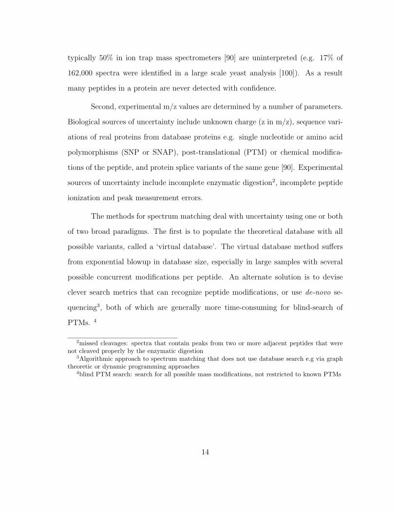
spectra from a complex mixture of proteins is shown in Figure 2.1. An MS/MS

peptide fragmentation spectrum (PFF) is generated for each peptide and contains

the m/z values for every fragment, along with the corresponding fragment intensity.

10

Protein identification

Database search

ATMNPKFMSRNQWFFSKATMNWKFSKNMTFRSKATLSPKFSSKNQWPFSW…ATPKFMS

MS1 MS2

Digested peptides MS/MS Spectra

(1) ATMNPK (4) NMTFRSK (3) ATMNWKFSK (2) NQWFFSK (6) ATLSPKFSSK

MS Spectrum

NQWFFSK

NMTFRSK ATMNWKFSK

ATMNPK

ATLSPKFSSK

Identified proteins

Peptide Database

One protein from a complex sample

Peptide identification

Mass spectrometry experiment

1: ATMNPKFMSRNQWFFSKATMNWKFSKNMTFRSKATLSPKFSSKNQWPFSW…ATPKFMS 2: AMFWSTKSMYSSQMWNLATMNWKFSKNWMFSKATLSPKFLSKNMWPSSW

Figure 2.1: A complex sample of proteins can generate on the order of 105 exper-imental MS/MS spectra. The figure depicts MS/MS spectra for one such protein.In bottom-up spectrometry, enzymes digest proteins into pieces called peptides (reddelimiter). In a first level of mass spectrometry (MS1), the peptides are ionizedand their mass-to-charge ratio is measured (MS1 spectrum). In the second levelof mass spectrometry (MS2), each peptide ion is further shattered into fragments.The list of m/z fragments from one peptide is one MS/MS spectrum. A databasesearch matches experimental spectra to theoretical spectra. Peptides that matchto experimental spectra are identified as being present in the sample. In turn, aprotein’s presence is inferred based on identification of one or more of its peptides(amino acids in bold font).

11

Since multiple copies of a protein (peptide) generally exist in the sample, multiple

PFF spectra are generated per peptide, each with a slightly differing peak list due

to experimental noise and possibility of post-translational modification. Again, the

peptide fragmentation process can be simulated in-silico to generate a database of

theoretical PFF spectra from known protein sequences. PFF spectra are mapped

to peptides using database lookup as described in Section 2.2. An MS/MS database

hit is called a Peptide Spectrum Match (PSM).

Tandem mass spectrometry (MS/MS) is much more effective for high-throughput

identification. A few unique PSMs are usually considered to be enough to confi-

dently identify the parent protein from among thousands of proteins in a sample.

This dissertation focuses on analysis of tandem mass spectrometry (MS/MS) data.

2.1.1 Mass spectrometry biases

Both peptides and proteins can be masked by mass spectrometry biases.

Mass spectrometers are less sensitive to low abundance proteins, and some peptides

never get ionized or generated into spectra, thus masking their presence and reducing

the percentage of a protein sequence that is identified (sequence coverage). If enough

peptides are not identified per protein, the entire protein itself can be masked1.

2.2 Mass spectrometry via database search

A typical MS/MS experiment generates tens of thousands of PFF spectra

from a sample containing a few thousand proteins e.g 30,000 spectra for an E. coli

sample (E.coli has ∼ 4000 genes). Spectra are unordered lists of mass-charge ratios

1experiment coverage: percentage of expected proteome that is identified

12

(m/z) since the ordering of amino acids is partially lost during fragmentation.

Figure 2.1 illustrates the process of MS/MS protein identification via database

lookup. The computational task is to map every MS/MS experimental spectrum to

a known peptide sequence, ultimately identifying a protein by identifying its con-

stituent peptides. When database lookup is used for the spectrum-peptide matching

step, the theoretical spectra database is generated from known protein sequences

using options that mirror the experimental setup.

2.2.1 Uncertainty in database lookup

Though the concept of database lookup is simple, the parameter space in-

volved in computationally simulating enzymatic digestion, ionization and fragmen-

tation of protein sequences is quite large. Moreover, since multiple variants of the

same peptide can exist in the sample, the database and/or search strategy must

include both unmodified and modified variants of the peptide, often resulting in

similar but distinct spectral signatures. Large search spaces increase both search

time and chances of a random incorrect match.

Further, spectra are high-dimensional (∼40,000 resolvable peaks) and 99.9%

sparse with only a few hundred peaks per spectrum. Nearest neighbor search in high-

dimensional, sparse space is an NP-hard problem [12]. The search is also necessarily

approximate for a number of reasons as described below.

First, experimental spectra are very noisy. Peptide shattering (fragmenta-

tion) is not a completely deterministic and completely understood process, and it

is prone to experimental variations and errors. As a result the fragmentation pro-

cess cannot be exactly simulated in the database, and theoretical spectra are not

exact replicas of experimental spectra. A large fraction of all experimental spectra,

13

typically 50% in ion trap mass spectrometers [90] are uninterpreted (e.g. 17% of

162,000 spectra were identified in a large scale yeast analysis [100]). As a result

many peptides in a protein are never detected with confidence.

Second, experimental m/z values are determined by a number of parameters.

Biological sources of uncertainty include unknown charge (z in m/z), sequence vari-

ations of real proteins from database proteins e.g. single nucleotide or amino acid

polymorphisms (SNP or SNAP), post-translational (PTM) or chemical modifica-

tions of the peptide, and protein splice variants of the same gene [90]. Experimental

sources of uncertainty include incomplete enzymatic digestion2, incomplete peptide

ionization and peak measurement errors.

The methods for spectrum matching deal with uncertainty using one or both

of two broad paradigms. The first is to populate the theoretical database with all

possible variants, called a ‘virtual database’. The virtual database method suffers

from exponential blowup in database size, especially in large samples with several

possible concurrent modifications per peptide. An alternate solution is to devise

clever search metrics that can recognize peptide modifications, or use de-novo se-

quencing3, both of which are generally more time-consuming for blind-search of

PTMs. 4

2missed cleavages: spectra that contain peaks from two or more adjacent peptides that werenot cleaved properly by the enzymatic digestion

3Algorithmic approach to spectrum matching that does not use database search e.g via graphtheoretic or dynamic programming approaches

4blind PTM search: search for all possible mass modifications, not restricted to known PTMs

14

2.3 Stages of computational protein identification

The three stages to protein identification via mass spectrometry are: (a)

spectrum-peptide matching (PSM), (b) peptide identification, by combining evi-

dence from several PSMs, (c) protein identification, by combining evidence from

peptide identifications.

The MS/MS datasets used in this dissertation were generated via a software

pipeline consisting of SEQUEST (BioWorks) [146] for spectra matching, Peptide-

Prophet [61] for peptide probabilities and ProteinProphet [89] for protein proba-

bilities. PeptideProphet and ProteinProphet are part of a software pipeline called

TransProteomic Pipeline (TPP, [60]).

2.3.1 Spectra matching

There are both frequentist [79, 101, 146] and Bayesian approaches [151] to

scoring spectrum matches. Many database lookup algorithms do not use the peak

intensities, and only rely on the m/z ladder. Frequentist approaches associate each

peptide spectrum match (PSM) with a similarity score and an expectation-value

(e-value, much like p-values). BioWorks’ SEQUEST is a commercial package based

on SEQUEST [146], which generates a PSM score based on a number of similarity

measures like cross-correlation (XCorr), and the XCorr difference between the top

and second-ranked peptide match (details are proprietary). Mascot is another pop-

ular proprietary package that is based on MOWSE scoring [96], which generates an

e-value for assessing statistical significance of every PSM.

More recently, open source versions like CRUX [97] and X!Tandem [19] have

become popular. CRUX re-implements and extends the SEQUEST engine for spec-

tral matching, adding a peptide indexing scheme to speedup searches. Despite

15

several other PSM algorithms in the literature [32, 58, 86], BioWorks and Mascot

remain the most widely-used in part because they ship with the instrument and are

well-supported by instrument manufacturers.

ProFound [151] adopts a Bayesian scoring scheme for matching PMF spec-

tra, computing the posterior probability P (+prot|peak matches) based on Gaussian

ditributed errors. In a survey of three systems for PMF matching, ProFound gave

the largest number of correct identifications [11]. Section 7.6 of this dissertation

extends ProFound’s scoring scheme to be applicable to MS/MS spectra for use in

MSFound.

2.3.2 Peptide identification

Database lookup generates a ranked list of PSMs for every experimental

MS/MS spectrum. There is an N:1 relationship between experimental spectra and

top-hit peptides. Multiple copies of a peptide can exist in the sample, and can

generate experimental spectra that map back to the same peptide in the database.

PeptideProphet [61] is a peptide-identification software (part of TPP). The

initial version used a mixture model to compute the probability of a correct peptide

identification P (+pep|Spep, E) given the evidence from a Peptide Spectrum Match

(Equation 2.1). PeptideProphet first uses linear discriminant analysis (LDA) to

generate a combined score Spep from multiple features of a PSM. For instance if SE-

QUEST is used for spectra matching, PeptideProphet uses features such as XCorr

and delta-correlation. The first version of PeptideProphet modeled the likelihood

of correct peptide identification P (Spep|+) as a Gamma distribution, and the nega-

tive identification likelihood P (Spep|−) as a Gaussian distribution with parameters

16

learned by expectation maximization (EM) and a ground-truth set of PSMs.

P (+pep|S,E) =π1f1(S,E)

π0f0(S,E) + π1f1(S,E)(2.1)

CRUX is another software that reports peptide probabilities and False Dis-

covery Rates via a semi-supervised learning method called Percolator [52]. Instead

of using a single ground-truth set and a fixed parametric model, Percolator dy-

namically learns true and null score distributions for every experiment by searches

against a decoy database of shuffled peptides (see Section 2.4.1). The null distribu-

tion is used to estimate peptide False Discovery Rates and q-values [56]. Recently,

PeptideProphet was also updated to learn the null component f0 per experiment

using a database of shuffled peptides [14].

2.3.3 Protein identification

After a set of unique peptides has been identified, they must be mapped to

proteins. This step is called the protein inference problem. In general, proteins with

multiple identified peptides are more likely to be present in the sample than proteins

with a single peptide identification (single-hit protein). A protein consists of several

peptides, and a peptide sequence can be shared across several proteins. The latter

is dubbed the degenerate peptide problem. The peptide-protein relationship is thus

of cardinality M : N .

ProteinProphet [89], the protein identification component of the TPP, com-

bines the peptide probabilities from PeptideProphet (Equation 2.1) into a protein

identification probability P (+prot). The protein probability is estimated as the prob-

ability of at least one peptide identification being correct, treating peptide identi-

fications as independent events. In Equation 2.2, maxj(P (+pep|Spepij, Ei)) is the

17

highest scoring of j PSMs for peptide i.

P (+prot) = 1−n∏i=1

(1−maxj(P (+pep|Spepij, Eij))) (2.2)

ProteinProphet also boosts an individual peptide’s identification probability

if other peptides from the parent protein are identified. These peptides are called

sibling peptides, and the adjustment is dubbed the neighboring sibling peptide ad-

justment (NSP). ProteinProphet also adjusts for peptides that belong to more than

one protein, called degenerate peptides, by weighting their identification probability

among the different parent proteins. ProteinProphet starts with uniform weights

and iteratively adjusts them based on the confidence in identification of each par-

ent protein in an EM-like manner. NSP-adjusted peptide probabilities and protein

probabilities are also updated iteratively till convergence.

For the past decade, the ProteinProphet has been the only available method

that estimates protein probabilities, and not due to lack of research on the problem.

Estimating statistical significance of protein inference is very hard due to the absence

of a good ground truth (or null model). Other widely used systems like DTASelect2

[129] allow the user to set various peptide score filters to narrow the list of ’good’

protein identifications, but do not provide protein-level scores or error rates. Very

recently, [113] published their system called MAYU to estimate protein-level FDRs

from protein scores. MAYU was not available at the time of developing the methods

described in this dissertation, and has not been tested in our experiments. All data

used in this dissertation was generated using the TPP.

18

2.4 Experimental evaluation of MS/MS experiments

This section describes evaluation in the absence of a ground-truth set, both

at the peptide and protein level. Peptide and protein identification scores must

be accompanied by statistical significance measures, especially if they are not true

probabilities. A well-defined null hypothesis, and a corresponding distribution of

null scores are both required to estimate p-values or False Discovery Rates. This

section summarizes the different strategies used to estimate null score distributions

for peptide identification. The target-decoy strategy described below performs well

and has become the de facto standard at the peptide level. However, good error

estimation at the protein level is still an open issue [54, 128] and an active area of

research.

2.4.1 Control mixtures and shuffled databases

Peptide-level error estimation strategies are based on searching against a

decoy peptide database. Any PSM to a decoy peptide is considered to be an incorrect

match, and the PSM score contributes to the null score distribution. The set of

proteins in the sample are called target proteins, and the theoretical database created

from target protein sequences is called the target database.

The decoy database can either be constructed from artificial protein se-

quences (shuffled proteins) or real protein sequences from an organism that did

not contribute to the sample [62] (control mixture). Since decoys are proteins from

another organism, they have an amino acid distribution that is typical of real pro-

teins and act as a stringent error measure. This disadvantage is that extensive

sequence similarity between target and decoy peptides can result in correct hits to

decoy peptides, and skew the null scores. For this reason, artificial decoy protein

19

sequences are generally used. Artificial proteins are derived from the target protein

sequences by random shuffling or reversal, or generated using a Markov model with

parameters learned from target sequences [16].

The above approaches do not account for random matches to target proteins,

since this aspect is much harder to model. One heuristic is to treat target proteins

that were identified based on a single peptide identification (single-hit proteins)

as incorrect identifications, since empirical observation shows that proteins with

multiple identified peptides are more likely to be true identifications [89]. We used

this heuristic in Chapter 4.

One may generate protein FDRs by running TPP (ProteinProphet) on a

shuffled database, and treating the shuffled identified proteins as false hits. In our

experiments, the resulting probabilities have a well-behaved uniform null p-value

distribution (Figure 4.9), but very high protein-FDRs, as confirmed by [113], who

show that using peptides with a given target-decoy FDR threshold=x% results in

FDR>x% at the protein level.

2.4.1.1 Concatenated vs. separate decoy database

In general there are two variations of the target-decoy search. One variant

uses a single search against a concatenated database of target and decoy sequences

[31], and the other uses separate searches against target and decoy databases [55].

Clearly the issue is misleading when framed as a choice of database search strat-

egy, since concatenated database searches are equivalent to separate searches if one

considers all decoy and target peptides identified per spectrum and not just the top-

scoring peptide. Rather, the choice must be driven by any statistical assumptions

made at the post-search statistical significance step [55]. The pros and cons of either

20

approach are discussed below, with details in [15,31,36,55].

Choi and Nesvizhskii [15] correctly point out that a separate search with a

naive estimation of FDRsimple = Nd/Nt, where Nd is the number of decoy PSMs and

Nt is the number of target PSMs, will overestimate Nd as it includes decoy PSMs

for spectra that already have a high-scoring target PSM in the target database

search. Separate search approaches must correct for this phenomenon by multiply-

ing FDRsimple by the expected proportion of incorrect peptide assignments in the

target database search [54]. Concatenated database searches correct for this phe-

nomenon to some extent, by only considering decoy PSMs that win the target-decoy

competition for every spectrum [15]. However, restricting the null distribution to

decoy PSMs that win the target-decoy competition may not be accurately reflect

the significance of a database search result [55]. Currently, we believe most searches

are carried out on concatenated databases [15], but the choice should depend on the

error estimation procedure used by the analysis software.

2.5 Evaluation metrics and terminology

Table 2.5 contains a list of evaluation measures used in this dissertation, along

with common abbreviations and definitions. ROC and Precision-Recall curves and

their utility are discussed below.

A Receiver Operator Characteristic (ROC) curve is a plot of True Positive

Rate vs. False Positive Rate (TPR, FPR, Table 2.5). The Area Under the ROC

curve (ROC-AUC or simply AUC) is a single number to compare different classifiers

evaluated on the same ground-truth and test data. A Precision-Recall curve is a

plot of True Positive Rate (TPR, Recall) vs. Precision (1-FDR). The area under the

21

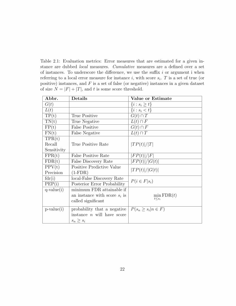
Table 2.1: Evaluation metrics: Error measures that are estimated for a given in-stance are dubbed local measures. Cumulative measures are a defined over a setof instances. To underscore the difference, we use the suffix i or argument i whenreferring to a local error measure for instance i, with score si. T is a set of true (orpositive) instances, and F is a set of false (or negative) instances in a given datasetof size N = |F |+ |T |, and t is some score threshold.

Abbr. Details Value or EstimateG(t) {i : si ≥ t}L(t) {i : si < t}TP(t) True Positive G(t) ∩ TTN(t) True Negative L(t) ∩ FFP(t) False Positive G(t) ∩ FFN(t) False Negative L(t) ∩ TTPR(t)

True Positive Rate |TP (t)|/|T |RecallSensitivityFPR(t) False Positive Rate |FP (t)|/|F |FDR(t) False Discovery Rate |FP (t)|/|G(t)|PPV(t) Positive Predictive Value |TP (t)|/|G(t)|Precision (1-FDR)fdr(i) local-False Discovery Rate

P (i ∈ F |si)PEP(i) Posterior Error Probabilityq-value(i) minimum FDR attainable if

an instance with score si iscalled significant

mint≤si

FDR(t)

p-value(i) probability that a negativeinstance n will have scoresn ≥ si

P (sn ≥ si|n ∈ F )

22

Precision-Recall curve is a a single number that estimates average precision across all

levels of recall [80]. We use the abbreviation PR-AUC to distinguish area under the

Precision-Recall curve from ROC-AUC. Between them, ROC and Precision-Recall

curves represent all four error quadrants: TPR, FPR and FDR, and the fourth

quadrant, False Negative Rate, which is (1-TPR).

Precision (1-FDR) answers this question:‘how many of the reported signifi-

cant hits are truly significant’, which is often the important question for proteomics

studies that only consider proteins above a significance threshold to be present in

the sample. However, ROC and ROC-AUC are important algorithmic measures

since AUC is a measure of the ability of the classifier to rank a randomly chosen

positive instance higher than a randomly chosen negative instance ( [34], AUC=0.5

for a classifier that classifies instances randomly). We present both Precision-Recall

and ROC curves in this research, and also report the number of proteins identified

at a 5% FDR cutoff. The choice of which is more relevant is dependent on the

application.

2.5.1 Literature-based ground truth

When available, good protein reference sets are very valuable to evaluate new

algorithms and error estimation methods. To facilitate the evaluation of the compu-

tational methods in this dissertation, we assembled one of the first comprehensive,

proteome-level reference sets for yeast grown in in rich and minimal media. Details

are in Chapter 3.

23

2.5.2 Error estimation without ground-truth

Whenever possible, this dissertation presents methods for estimating sta-

tistical significance in the absence of ground truth e.g. using random models to

generate a statistical null hypothesis, or using function analysis5 to detect outliers6

(see evaluation sections in Chapters 4 and 5).

2.5.3 False Discovery Rates in genomic and proteomic literature

This section presents a history of false discovery rates in the early computa-

tional genomics and proteomics literature, and attempts to clarify any ambiguity in

the terminology. False discovery rate (FDR) is defined as the Type II error over a

set of data points called significant. Local-fdr is the probability of a false-positive at

a particular data point when it is called significant. The term ‘local-fdr’ was derived

from the original definition of FDR by Benjamini and Hochberg [5] for multiple

hypothesis testing. local-fdr is equivalent to the posterior error probability of an

instance in the Bayesian setting [55].

Efron et al [30] and Storey et al [126] were the first studies to systematically

address FDR and local-fdr in the large-scale gene expression literature. Efron et al

estimated the local-fdr by modeling a mixture model approach with an exponential

distribution for the non-null component. Storey et al detailed a semi-parametric

approach that used the expected uniform distribution of null p-values to determine

the percentage of null (random) hits from a histogram of p-values. Scheid and Spang

[118] presented a method to improve the estimated null distribution by selecting

5estimate the set of biological functions that are enriched for the set of identified proteins [114]6A biological function that is not expected in the sample might indicate some spurious protein

identifications

24

only a subset of permutation tests that result in uniform p-value distributions. Kall

et al [56] used an approach derived from Storey et al to estimate q-values and

posterior error probabilities (PEP) given true and null score distributions of peptide

spectrum matches. It is worth noting that all the above approaches assume that all

the hypothesis tests are independent; which need not necessarily hold for hypotheses

tests of individual gene or protein presence [126].

25

Chapter 3

Datasets and benchmarking

3.1 Protein and mRNA datasets

This dissertation introduces and uses a comprehensive set of benchmark-

ing data for computational proteomics. This chapter is a reference to all test and

ground-truth data used in Chapters 4, 5 and 6. All proteomics MS/MS datasets

are summarized in Table 3.1. mRNA datasets are in Table 3.2. Collected protein

reference sets are summarized in Table 3.3 and further discussed in Section 3.2.

MS/MS protein identification was conducted using the BioWorks 3.3 (Ther-

moFinnigan), PeptideProphet and ProteinProphet (TransProteomic Pipeline). All

MS/MS datasets were run using multiple technical replicates unless mentioned oth-

erwise. A technical replicate is a repeated experiment on the same biological sample

(different injections of the same sample), and controls for variability of the exper-

imental analysis. A biological replicate is a repeated experiment on a biological

sample from a different source (different cell line, patient, or biopsy), and controls

for biological variability. Sample preparation details are in the MSPresso [111] and

MSNet publications [110].

3.1.1 Yeast

The yeast datasets are most comprehensive: across different mass spectrom-

eters, sample complexity (number of expected proteins) and sample conditions.

26

3.1.1.1 Yeast grown in rich medium

A whole cell lysate1 of yeast grown in rich medium was analyzed on two

different mass spectrometers: a low-resolution LCQ mass spectrometer (YPD-LCQ),

and a high-resolution LTQ-OrbiTrap mass spectrometer (YPD-ORBI). The mRNA

abundance for every gene was computed as the average value from three independent

gene expression experiments when at least two experiments had observed mRNA

for that gene, and zero otherwise. The three mRNA experiments were derived from

wild-type yeast grown to log-phase in rich medium [49,133,137].

3.1.1.2 Yeast grown in rich medium, polysomal fraction

A fractionation experiment (sucrose gradient) that isolated 80S ribosomal

proteins from a sample of yeast grown in rich medium was analyzed on the LCQ

mass spectrometer (Table 3.1, YMD-LCQ-Fraction). The mRNA data was derived

from the rich-medium yeast datasets described above.

3.1.1.3 Yeast grown in minimal medium

Whole cell lysate of yeast grown in minimal medium was analyzed on the LCQ

mass spectrometer, with mRNA abundance from [125] (Table 3.1, YMD-LCQ).

3.1.2 E. coli

A sample of E. coli grown in minimal medium was analyzed on an ORBI

mass spectrometer (Table 3.1, E. coli). Three datasets provided the corresponding

mRNA abundance [3, 17,18].

1lysis is the process of digesting a cell. Whole cell lysate experiments study all proteins presentin the cell, as opposed to fractionation experiments that study particular fractions of the proteome

27

3.1.3 Human

3.1.3.1 DAOY medulloblastoma cell line

A sample from the DAOY medulloblastoma cancer line was analyzed on LCQ

and ORBI mass spectrometers. Ten technical replicates (injections) of the MS/MS

experiment were run on the ORBI mass spectrometer. One replicate was used as

the test set (Table 3.1, Human-Daoy-ORBI), and confident identifications from the

other nine replicates were pooled into a protein reference set (≤ 5% FDR). One

injection from the sample was also analyzed on a low-resolution mass spectrometer

(Table 3.1, Human-Daoy-LCQ), and confident proteins from all ten ORBI replicates

were used as a reference set. No published high-throughput human proteomics data

was available as a reference set.

3.1.3.2 HEK293T kidney cells

One injection of protein extracts of human HEK293T cells (Table 3.1, Human-

293T) was analyzed on the ORBI mass spectrometer.

3.2 Benchmarking

Lack of ground-truth is typical in domains where data generation is much

faster and cheaper than experimental verification. An alternative to expensive bio-

logical validation is to estimate a notion of ground-truth from available data. How-

ever, though proteomics data is becoming publicly available (OPD [106], PRIDE

[85]), data integration is a non-trivial challenge due to several different storage and

data representation formats.

28

3.2.1 Literature-based reference sets

High-confidence protein identifications from different protein identification

technologies experiments might hold complementary information about a sample.

These high-confidence identifications can be assembled into a ground-truth protein

set per sample. For the such reference set to be a meaningful ground-truth, the

experiments should be carried out on the same sample of interest, using similar

experimental parameters. However, the noisy results of shotgun MS/MS experi-

ments from different mass spectrometers and analysis tools are notoriously hard to

replicate and consolidate. Even if the data is available, and contains a consensus,

assembly is tedious because MS/MS protein repositories use different representation

standards and storage formats.

We2 collected and curated data from several high-throughput proteomics ex-

periments in the literature to act as ground-truth sets in this dissertation. These

experiments were performed by different laboratories using different analysis meth-

ods on same or similar samples. For instance, for yeast grown in rich medium, we

collected eight protein identification experiments in the literature (dubbed reference

experiments). Five were based on MS/MS experiments and three were based on

non-MS methods. A core subset of high-confidence protein identifications from the

reference experiments forms the set of positive instances, and is referred to as the

protein reference set in this dissertation. We also collected reference sets for the

other yeast datasets, and (limited) reference data for the E. coli proteome. We

could not locate publicly available reference experiments that matched the human

MS/MS data in Table 3.1, which was expected given that human proteomics is still

2work with Christine Vogel

29

in very early stages of research.

Defining negative instances, i.e. proteins absent from the sample, was a

much harder problem since proteomics experiments have high false-negative rates.

One approach is to restrict the negative set to proteins that are not identified in

any reference experiment [110], since these proteins are more likely to be erroneous

identifications. However, since this approach loses proteins that are detectable by

certain experiments (technologies), we conservatively define the negative set as the

complement of the positive set. All reference sets are summarized in Table 3.3. The

yeast reference set for rich medium whole cell lysate is quite comprehensive and

covers most of the expressed yeast proteins (2/3 of the genome).

3.2.1.1 Constructing a benchmark set

To construct a consensus set from the rich-medium yeast data, we chose

proteins present in at least two of four MS-based experiments or at least one of three

non-MS-based experiments (YPD*). This selection was based on expert knowledge

and level of trust in the reliability of each experiment. The other reference sets in

Table 3.3 were similarly constructed.

An alternate scalable approach is to derive a consensus automatically using

clustering. For N reference experiments, each protein Pi can be represented as an

N -dimensional Boolean vector, P1×N , where Pij = 1 if protein i was observed with

high confidence in the jth experiment and zero otherwise. Expectation-Maximization

(EM) clustering [26] of proteins resulted in two clusters (present in sample, absent

from sample). Clusters were initialized by picking the initialization that minimized

the sum-squared error (SSE) of final clusters from ten runs of k-means clustering.

We used the default settings of the EM clustering algorithm in the Weka machine

30

learning toolbox ( [47], version 3.5.7).

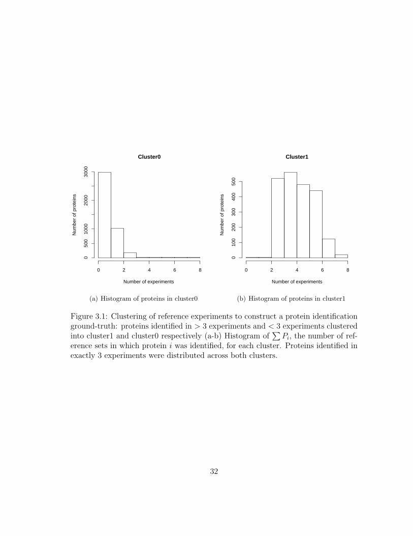
The protein clusters that resulted from EM-clustering can be described by

a simple rule: cluster1 had proteins that were confidently identified in ≥ three

experiments, and cluster0 had proteins that were confidently identified in ≤ three

experiments. Proteins identified in exactly three experiments were distributed across

the two clusters. Figure 3.1(a) and Figure 3.1(b) show histograms of proteins as-

signed to each cluster. Each histogram data point i is the number of experiments

that identified protein Pi (∑

i Pi). cluster1 was labeled as the ‘presence’ cluster.

Since different clusterings may hold information about proteins detectable by

different technologies, a consensus clustering paradigm may serve as an exploratory

tool and an alternative to EM-clustering (Chapter 8). However, cluster validation

is an elusive issue in the absence of ground truth. For instance, MSNet achieved a

similar percentage increase in AUC for both clustering-based and hand-crafted ref-

erence sets (see Chapter 5, Figure 3.1 and Figure 5.4). The experiments in Chapters

4-6 use the hand-crafted reference sets in Table 3.3.

3.3 Availability

All benchmarking data is publicly available. Protein reference sets for yeast

are available at http://marcottelab.org/MSData/Gold. MS/MS proteomics datasets

are available at http://marcottelab.org/MSData.

31

Cluster0

Number of experiments

Num

ber

of p

rote

ins

0 2 4 6 8

050

010

0020

0030

00

(a) Histogram of proteins in cluster0

Cluster1

Number of experiments

Num

ber

of p

rote

ins

0 2 4 6 8

010

020

030

040

050

0

(b) Histogram of proteins in cluster1

Figure 3.1: Clustering of reference experiments to construct a protein identificationground-truth: proteins identified in > 3 experiments and < 3 experiments clusteredinto cluster1 and cluster0 respectively (a-b) Histogram of

∑Pi, the number of ref-

erence sets in which protein i was identified, for each cluster. Proteins identified inexactly 3 experiments were distributed across both clusters.

32

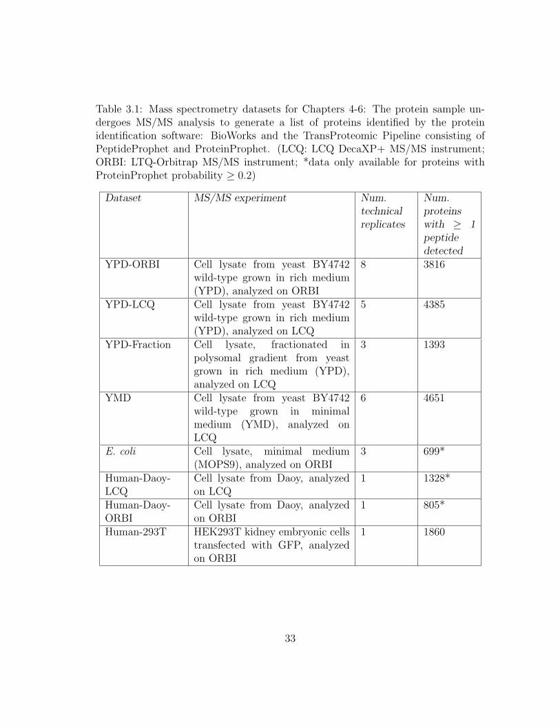
Table 3.1: Mass spectrometry datasets for Chapters 4-6: The protein sample un-dergoes MS/MS analysis to generate a list of proteins identified by the proteinidentification software: BioWorks and the TransProteomic Pipeline consisting ofPeptideProphet and ProteinProphet. (LCQ: LCQ DecaXP+ MS/MS instrument;ORBI: LTQ-Orbitrap MS/MS instrument; *data only available for proteins withProteinProphet probability ≥ 0.2)

Dataset MS/MS experiment Num.technicalreplicates

Num.proteinswith ≥ 1peptidedetected

YPD-ORBI Cell lysate from yeast BY4742wild-type grown in rich medium(YPD), analyzed on ORBI

8 3816

YPD-LCQ Cell lysate from yeast BY4742wild-type grown in rich medium(YPD), analyzed on LCQ

5 4385

YPD-Fraction Cell lysate, fractionated inpolysomal gradient from yeastgrown in rich medium (YPD),analyzed on LCQ

3 1393

YMD Cell lysate from yeast BY4742wild-type grown in minimalmedium (YMD), analyzed onLCQ

6 4651

E. coli Cell lysate, minimal medium(MOPS9), analyzed on ORBI

3 699*

Human-Daoy-LCQ

Cell lysate from Daoy, analyzedon LCQ

1 1328*

Human-Daoy-ORBI

Cell lysate from Daoy, analyzedon ORBI

1 805*

Human-293T HEK293T kidney embryonic cellstransfected with GFP, analyzedon ORBI

1 1860

33

Table 3.2: mRNA datasets for MSPresso (Chapter 4)

Dataset mRNA experiment(s) Num.expressedgenes

YPD-ORBI,YPD-LCQ,YPD-Fraction

Average mRNA abundance when gene is ex-pressed in ≥ 2 of 3 experiments [49,133,137]

5174

YMD Single channel microarray (Affymetrix) [125] 6014E. coli Average mRNA abundance when gene is ex-

pressed in ≥ 2 of 3 experiments [3, 17, 18]2470

Human-Daoy-LCQ, Human-Daoy-ORBI

Single channel microarray, unpublished (Pe-nalva O.L., Childrens Cancer Research Insti-tute; UT Health Science Center at San Anto-nio, TX)

13,340

Table 3.3: Protein reference sets for Chapters 4-6

Sample Protein reference set Number ofproteins

YPD-ORBI,YPD-LCQ

YP3: Proteins identified in≥ 1 of 3 non-mass spec-trometry experiments [38, 40,91]

4097

YP4: Proteins identified in ≥ 2 of 4 MS experi-ments [13,24,100,138]

1648

YPD*: YP3⋃

YP4 4264YPD-Fraction

Known ribosomal, translation and ribosome bio-genesis proteins [88,103]

593

YMD YMD*: Union of 3 experiments [24, 91,152] 2529E. coli Union of two 2D-gel electrophoresis experiments

[74,76]394

Human-Daoy-LCQ

10 injections of the same sample analyzed on ORBI 1477

Human-Daoy-ORBI

9 injections of the same sample analyzed on ORBI 1586

Human-293T No comprehensive protein reference set available -

34

Chapter 4

Integrative analysis of gene expression and

proteomics experiments

4.1 Introduction

The vast majority of MS/MS experiments are analyzed without consider-

ing any prior information regarding a protein’s presence in the sample. In reality,

other information may be readily available and can be used to influence the inferred

probability of protein presence when evidence from the MS/MS experiment is weak.

Direct evidence is generated by methods that measure protein presence e.g. MS/MS

analysis. Inferential evidence refers to data that implies protein presence but does

not directly measure it, e.g. mRNA abundance. For instance, since mRNA is tem-

poral precursor of protein, presence of mRNA from a particular gene may imply

presence of the associated protein.

Biological dogma states that proteins are created from mRNA, which is cre-

ated from DNA. In general, one can expect that proteins with high observed mRNA

abundance1 for the associated gene are more likely to be present than proteins for

which no mRNA was observed. mRNA expression levels are routinely measured

in a high-throughput manner using gene expression chips. Recently, Lu et al [77]

showed that that mRNA abundance can explain over 70% of variance in yeast protein

abundance and about half of the variance in E. coli protein abundance (confidently

1abundance or concentration: number of molecules/cell

35

detected proteins, Pearson correlation coefficient R2=0.73 for yeast, R2=0.47 for E.

coli).

Our method, MSPresso (for MS and expression data), integrates data from

MS/MS and mRNA experiments, using observed mRNA abundance as prior knowl-

edge for protein presence. To our knowledge, MSPresso is the first integrative ap-

proach to analysis of shotgun proteomics data. MSPresso studies the relationship

between protein presence (variable K = {0, 1}) and mRNA abundance M ∈ <.

This notion is different from the relationship between protein abundance and mRNA

abundance, another complex dynamic relationship that has been extensively studied

at large-scale as discussed in Section 4.6.

4.2 Methods

Bayesian methods are particularly suitable for data integration in noisy do-

mains, since it is conceptually easy to incorporate available data into the model

as prior knowledge. The MSPresso model illustrated in Figure 4.1 considers three

variables:

1. K = {0, 1}: represents a protein’s presence with probability P (K = 1)

2. M : continuous variable, represents absolute mRNA abundance (log-scale)

3. S: continuous variable, represents the MS/MS protein identification score

MSPresso estimates a Bayesian posterior protein identification probability P (K =

1|S = s,M = m) for each protein, the probability of protein K being present in

the sample having observed it in an MS/MS experiment with an identification score

36

(S=s), and having observed the associated gene’s mRNA abundance (M=m) under

similar experimental conditions:

P (K = 1|M = m,S = s) ≡ P (K|M,S) (4.1)

∝ P (K,M, S)

∝ P (S)P (K|S)P (M |K,S)

∝ P (S)P (K|S)P (M |K) (4.2)

∝ P (S)P (K|S)P (K|M)P (M)

P (K)

∝ P (S)P (M)P (K|M)P (K|S)

P (K)

=P (K|S)P (K|M)

P (K)/∑K=1,0

P (K|S)P (K|M)

P (K)(4.3)

Equation 4.2 uses a simplifying conditional independence assumption be-

tween M and S given K, setting P (M |K,S) = P (M |K). Other classifiers that do

not make a conditional independence assumption do not empirically outperform

MSPresso (Section 4.5.1). The protein identification probabilities S used in our

experiments also do not correlate well with protein or mRNA abundance (Section

4.5.2.3).

4.2.1 Estimating conditional probabilities

P (K|S): MSPresso trains a logistic regression classifier using protein score S

as the dependent variable and response variable K. P (K = 1|S) is estimated as the

posterior probability of this classifier which is trained using the protein reference set

from Chapter 3 to define positive and negative instances.

P (K|M): MSPresso trains a model from experimentally determined mRNA

abundances and protein identifications collected from the reference datasets de-

37

MSpresso protein identification probability P(K=1|S=s,M=m)

P(K|S): trained on S and K or re-use of existing modelP(K|M): trained on M and K or re-use of existing modelP(K): uniform prior

Protein identification scores from

MS/MS experiment!S = {s}

Reference set astraining data for protein

presence/absence!K = {1,0}

mRNA abundances

from gene expressionexperiment!M = {m}

LC/LC-MS/MS spectraProtein extract

Search against spectrafrom peptide sequence

database

proteins peptides

Figure 4.1: Improving protein identification rates using observed mRNAabundance as prior information of protein presence: MS/MS analysis on acomplex protein sample produces a ranked list of identified proteins with a confi-dence score for each protein (S). A gene expression experiment on the same, or sim-ilar, sample generates an observed mRNA abundance for expressed genes (M). MS-Presso estimates the posterior probability of protein K’s presence, P (K = 1|S,M),given that it was detected in the MS/MS experiment with score S = s, and had thecorresponding gene expressed in the mRNA experiment with abundance M = m.MSPresso estimates three probability distributions: P (K|S), P (K), and P (K|M)

38

0

0.1

0.2

0.3

0.4

0.5

0.6

0.7

0.8

0.9

1

-3 -2 -1 0 1 2 3 4 5 6

P(K

=1|

M)

mRNA concentration (mol/cell, log scale)

(a) mRNA abundance averaged over three exper-iments

0

0.1

0.2

0.3

0.4

0.5

0.6

0.7

0.8

0.9

1

-3 -2 -1 0 1 2 3 4 5 6

P(K

=1|

M)


mRNA-SAGEmRNA-HDA

mRNA-WangmRNA-Avg-2of3

(b) mRNA abundance from each experiment sep-arately

0

0.1

0.2

0.3

0.4

0.5

0.6

0.7

0.8

0.9

1

-3 -2 -1 0 1 2 3 4 5 6

P(K

=1|

M)


(c) Including membrane proteins

0.5

0.6

0.7

0.8

0.9

1

0 100 200 300 400 500 600 700 800 900 1000

AU

C

mRNA bin size

AUC-ROCAUC-PR

(d) Choosing bin size for P (K|M)

Figure 4.2: Estimating P (K|M) for yeast grown in rich medium using mRNA datafor YPD-LCQ from Table 3.2 and the YP4 protein reference set from Table 3.3(cross-validated estimates for each data point (protein) are plotted) (a) when mRNAabundance M is the average from three experiments, yeast membrane proteins ex-cluded. The step-function is conserved when (b) using each mRNA experimentindividually and (c) including membrane proteins (d) performance of MSPresso isnot sensitive to P (K|M) bin size (data same as (a))

39

14

Figure S1. Estimating P(K)

REF-MS

1498 (30%)

REF-non-MS

3443 (69%)

mRNA

4165

(83%)

To

tal: 4

96

2

MS ! mRNA:1433 (29%)

Non-MS ! mRNA:3203 (66%)

1286

MS:

1647

Non-MS:

4097

mRNA:

5197

Total: 6331

MS ! mRNA:1580

Non-MS ! mRNA:3820

1417

A. Excluding membrane proteins

B. Including membrane proteins

Legend:

MS MS-based reference set

Non-MS Non-MS-based reference set

mRNA mRNA dataset

(A) Of a total of 4962 yeast proteins without membrane helices, 3443 proteins (69%)

are observed in the non-MS-based protein reference set, 1498 (30%) in the MS-

based reference set. Both estimates are likely conservative given that the fraction of

expressed mRNAs is even larger than 2/3 (4165 of 4962 genes; 83%). When

computed over only proteins with detected mRNA abundances, the estimates are

larger: e.g., of 4165 total proteins without membrane helices that also have detected

mRNA abundances, 77% are present in the non-MS based protein reference set

and 34% are present in the MS-based reference set.

(B) Corresponding numbers including membrane proteins.

Figure 4.3: To estimate P (K), theprior probability of protein presence(Equation 4.3), we investigate the over-lap between mRNA and protein iden-tification experiments (reference sets).We set P(K)=66%, based on theintersection of the mRNA and thenon-mass-spectrometry protein refer-ence sets (REF-non-MS).

scribed in Chapter 3. The protein reference set YP4, based on mass spectrometry

experiments, is used as ground-truth for training and evaluation on rich-medium

yeast samples (see Table 3.3). P (K = 1|M) is estimated by binning the mRNA

values, with equal number of data points per bin. P (K = 1|M = m) is estimated

by the percentage of proteins in the bin representing M = m that are present in

the reference dataset. Bin width is chosen to maximize the ROC Area Under Curve

(ROC-AUC) using cross-validation. In general, performance of the MSPresso clas-

sifier, measured by area under ROC and Precision-Recall curves, was not sensitive

to bin size (Figure 4.2(d)).

As expected, P (K = 1|M) increases with increasing mRNA abundance. In

yeast, Figure 4.2(a) resembles a step function with linear interpolation between

steps: below a (log-scale) abundance of about 0.5 mRNA molecules/cell the proba-

bility of the protein being present in the reference set is low (P(K=1—M) ≤ 0.10),

while above nine molecules/cell the probability is high (P(K=1) ≥ 0.90). The step

function is conserved across different sample conditions in yeast, as well as across

organisms (Figure 4.4).

40

P (K): Prior probability P (K) is set to a uniform prior. MSPresso uses

P (K = 1) = 2/3 since about two-thirds of all yeast proteins are expected to be

present in the sample. As depicted in the Venn diagram of Figure 4.3, this fraction

is consistent with the overlap between the yeast protein reference dataset that is

not based on mass-spectrometry (YP3, Table 3.3) and the set of observed mRNA

abundances M.

4.3 Results

MSPresso is applicable to a variety of organisms, sample conditions and mass

spectrometers: from whole-cell lysates (all proteins) to cellular fractions (subset of

proteins focus on particular cellular locations). Dataset details are in Section 3.1.

The experiments in this section use protein reference sets for training and evaluation.

MSPresso probabilities were averaged over ten runs of ten-fold cross-validation to

avoid over-fitting to the reference set.

Test Set: For every dataset in Table 3.1, the test set consisted of proteins

with both MS/MS and mRNA evidence (no missing data imputation), excluding

proteins with any predicted membrane2 helices [53]. Including transmembrane pro-

teins gave results with similar trends (Figure 4.5), and the protein-mRNA relation-

ship was also conserved (Figure 4.2(c)).

MSPresso computed a protein identification probability for every test set

protein using Equation 4.3. MSPresso increased the number of identifications at

5%FPR by 19 to 63% across all datasets (Table 4.1), while maintaining constant or

higher precision than the MS/MS identification (Figure 4.5(b)). MSPresso increased

2Since the samples were extracted from the cellular cytosol, proteins from the cellular membraneare not expected to be present

41

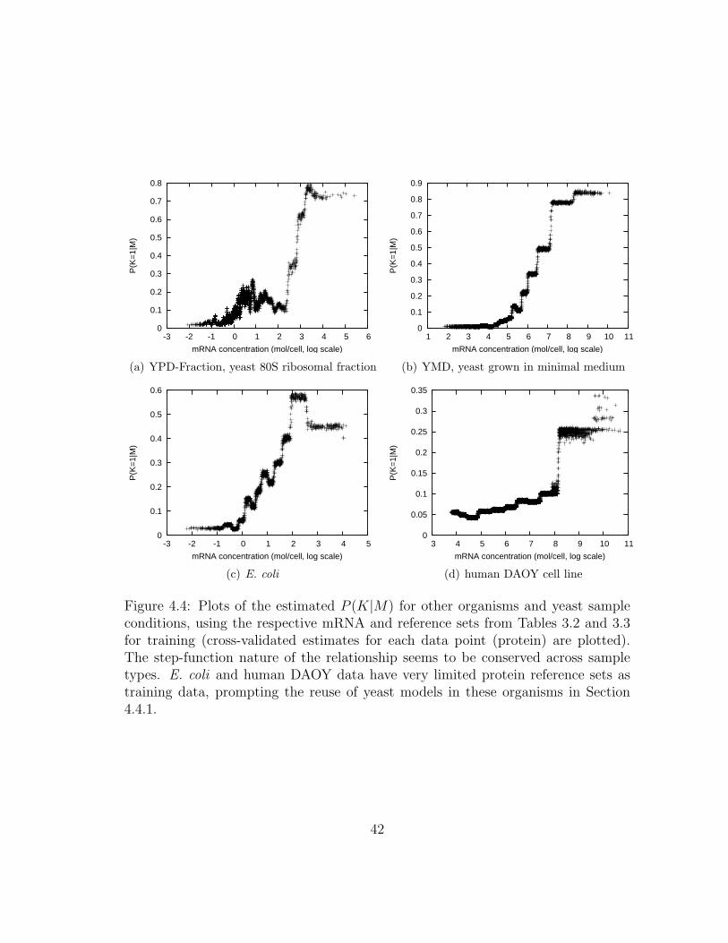
0

0.1

0.2

0.3

0.4

0.5

0.6

0.7

0.8

-3 -2 -1 0 1 2 3 4 5 6

P(K

=1|

M)


(a) YPD-Fraction, yeast 80S ribosomal fraction

0

0.1

0.2

0.3

0.4

0.5

0.6

0.7

0.8

0.9

1 2 3 4 5 6 7 8 9 10 11

P(K

=1|

M)


(b) YMD, yeast grown in minimal medium

0

0.1

0.2

0.3

0.4

0.5

0.6

-3 -2 -1 0 1 2 3 4 5

P(K

=1|

M)


(c) E. coli

0

0.05

0.1

0.15

0.2

0.25

0.3

0.35

3 4 5 6 7 8 9 10 11

P(K

=1|

M)


(d) human DAOY cell line

Figure 4.4: Plots of the estimated P (K|M) for other organisms and yeast sampleconditions, using the respective mRNA and reference sets from Tables 3.2 and 3.3for training (cross-validated estimates for each data point (protein) are plotted).The step-function nature of the relationship seems to be conserved across sampletypes. E. coli and human DAOY data have very limited protein reference sets astraining data, prompting the reuse of yeast models in these organisms in Section4.4.1.

42

Table 4.1: In each experiment, MSPresso scores were generated for every non-membrane protein with observed mRNA abundance and MS/MS identificationscore. These results use the self MSPresso model: trained and evaluated onexperiment-specific protein reference set (Table 3.3). MSPresso (MSP) improvesROC-AUC over the MS/MS experiment (MS) by 3-19%, and increases the numberof proteins identified at 5% FPR by 19-63% across datasets.(*data interpolated fromROC curve where there was no data at 5% FPR)

Experiment ROC-AUC Number of proteins at 5% FPRMS MSP % Increase MS MSP % Increase

YPD-LCQ 0.75 0.89 19 234 327 40YPD-ORBI 0.80 0.84 5 428* 618 63YMD 0.73 0.84 15 229 278 21Yeast-Fraction 0.72 0.77 7 21* 34 62E. coli 0.69 0.80 16 63* 87 38Human-Daoy-LCQ 0.71 0.75 6 99 121 22Human-Daoy-ORBI 0.79 0.81 3 105 125 19

ROC-AUC by 3 to 19% across experiments; a substantial increase since ROC-AUC

is the probability of correct classification of a randomly chosen correct instance over

a randomly chosen incorrect one. Table 4.1 summarizes the results at 5% FPR all

datasets. Detailed results for each dataset are described below.

4.3.1 Yeast

4.3.1.1 Yeast grown in rich medium

This section describes results on a sample of yeast grown in rich medium,

analyzed on an LCQ mass spectrometer (YPD-LCQ, Table 3.1). MSPresso iden-

tified more proteins at the same error rate than the MS/MS experiment. Figure

4.5 contains ROC and Precision-recall curves for proteins identified based only on

MS/MS data, only on mRNA abundance and based on both data sources (pro-

teins ranked by S and P (K = 1|S), by P (K = 1|M), and by MSPresso probability

43

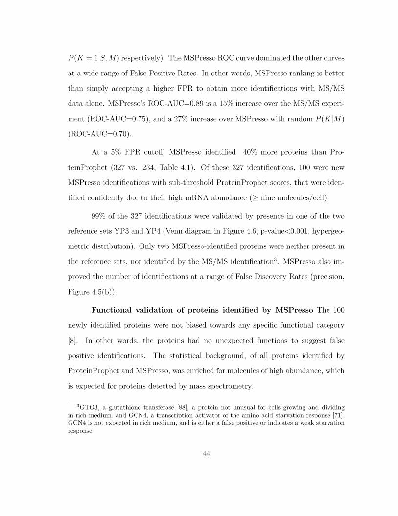
P (K = 1|S,M) respectively). The MSPresso ROC curve dominated the other curves

at a wide range of False Positive Rates. In other words, MSPresso ranking is better

than simply accepting a higher FPR to obtain more identifications with MS/MS

data alone. MSPresso’s ROC-AUC=0.89 is a 15% increase over the MS/MS experi-

ment (ROC-AUC=0.75), and a 27% increase over MSPresso with random P (K|M)

(ROC-AUC=0.70).

At a 5% FPR cutoff, MSPresso identified 40% more proteins than Pro-

teinProphet (327 vs. 234, Table 4.1). Of these 327 identifications, 100 were new

MSPresso identifications with sub-threshold ProteinProphet scores, that were iden-

tified confidently due to their high mRNA abundance (≥ nine molecules/cell).

99% of the 327 identifications were validated by presence in one of the two

reference sets YP3 and YP4 (Venn diagram in Figure 4.6, p-value<0.001, hypergeo-

metric distribution). Only two MSPresso-identified proteins were neither present in

the reference sets, nor identified by the MS/MS identification3. MSPresso also im-

proved the number of identifications at a range of False Discovery Rates (precision,

Figure 4.5(b)).

Functional validation of proteins identified by MSPresso The 100

newly identified proteins were not biased towards any specific functional category

[8]. In other words, the proteins had no unexpected functions to suggest false

positive identifications. The statistical background, of all proteins identified by

ProteinProphet and MSPresso, was enriched for molecules of high abundance, which

is expected for proteins detected by mass spectrometry.

3GTO3, a glutathione transferase [88], a protein not unusual for cells growing and dividingin rich medium, and GCN4, a transcription activator of the amino acid starvation response [71].GCN4 is not expected in rich medium, and is either a false positive or indicates a weak starvationresponse

44

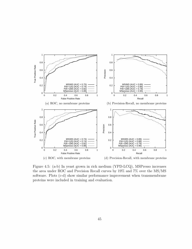
0

0.2

0.4

0.6

0.8

1

0 0.2 0.4 0.6 0.8 1

Tru

e P

ositi

ve R

ate

False Positive Rate

MS/MS (AUC = 0.75)P(K=1|S) (AUC = 0.74)P(K=1|M) (AUC = 0.82)MSpresso (AUC = 0.89)

(a) ROC, no membrane proteins

0

0.2

0.4

0.6

0.8

1

0 0.2 0.4 0.6 0.8 1

Pre

cisi

on

Recall


(b) Precision-Recall, no membrane proteins

0

0.2

0.4

0.6

0.8

1

0 0.2 0.4 0.6 0.8 1

Tru

e P

ositi

ve R

ate

False Positive Rate


(c) ROC, with membrane proteins

0

0.2

0.4

0.6

0.8

1

0 0.2 0.4 0.6 0.8 1

Pre

cisi

on

Recall


(d) Precision-Recall, with membrane proteins

Figure 4.5: (a-b) In yeast grown in rich medium (YPD-LCQ), MSPresso increasesthe area under ROC and Precision Recall curves by 19% and 7% over the MS/MSsoftware. Plots (c-d) show similar performance improvement when transmembraneproteins were included in training and evaluation.

45

188

1102147

3 2

1

32

9410

997 REF-non-MS

(3443)REF-MS

(1433)

MSPRESSOMS/MS

(234)

2 4

33 25

Validated MSpresso proteins (italic font)

(324/327 = 99%)

(327)

Figure 4.6: 99% of the 327 proteinsidentified by MSPresso at 5%FPR canbe validated by their presence in ei-ther the original MS/MS experiment,or the MS-based (YP4) or non-MS-based (YP3) protein reference sets.

As described in Section 3.1.1, the mRNA abundance for yeast was averaged

over three different mRNA experiments to account for experiment variability. How-

ever, the step-function trend of P (K|M) persisted when each of the three mRNA

experiments were used individually (Figure 4.2(b)).

4.3.1.2 Other yeast data

MSPresso was equally applicable to yeast in other sample conditions: YPD-

ORBI, YPD-LCQ-Fraction, and YMD datasets (rich medium on high-res mass spec-

trometer, yeast polysomal fraction, and minimal medium: Table 3.1). ROC and

Precision-Recall plots are in Figure 4.7, with MSPresso gaining 7-10% higher ROC-

AUC. Rich and minimal medium samples are expected to be significantly different

in their protein content, and the proteins rescued by MSPresso all had the expected

functional biases. YPD-ORBI and YMD experiments were strongly enriched for

46

0

0.2

0.4

0.6

0.8

1

0 0.2 0.4 0.6 0.8 1

Tru

e P

ositi

ve R

ate

False Positive Rate


(a) YPD-ORBI

0

0.2

0.4

0.6

0.8

1

0 0.2 0.4 0.6 0.8 1

Pre

cisi

on

Recall


(b) YPD-ORBI

0

0.2

0.4

0.6

0.8

1

0 0.2 0.4 0.6 0.8 1

Tru

e P

ositi

ve R

ate

False Positive Rate


(c) YPD-Fraction

0

0.2

0.4

0.6

0.8

1

0 0.2 0.4 0.6 0.8 1

Pre

cisi

on

Recall


(d) YPD-Fraction

0

0.2

0.4

0.6

0.8

1

0 0.2 0.4 0.6 0.8 1

Tru

e P

ositi

ve R

ate

False Positive Rate

MS/MS (AUC = 0.84)P(K=1|S) (AUC = 0.83)P(K=1|M) (AUC = 0.9)

MSpresso (AUC = 0.93)

(e) YMD

0

0.2

0.4

0.6

0.8

1

0 0.2 0.4 0.6 0.8 1

Pre

cisi

on

Recall


(f) YMD

Figure 4.7: MSPresso improves performance on other yeast datasets from Section3.1.1 (a-b) YPD-ORBI: rich-medium sample analyzed on a high-resolution OrbiTrapmass spectrometer (c-d) YPD-LCQ-Fraction: 80s ribosomal fraction (e-f) YMD:grown in minimal medium

47

metabolic and ribosomal functions (p-value<0.001) [8]. Proteins of these functions

are expected in high abundance in our samples which contain growing and dividing

yeast cells. MSPresso proteins from YMD were also enriched for small molecule

metabolism (p-value<0.001), which is consistent with growth in minimal medium.

Proteins identified in the ribosomal fractionation sample (YPD-Fraction-

LCQ) were enriched for ribosomal proteins, which is the expected result4. MSPresso

improved ROC-AUC by 7% for the smaller fractionation study, but did not improve

precision-recall AUC. MSNet in Chapter 5 results in better performance for this

fractionation data.

4.3.2 E. coli sample

E. coli data is described in Section 3.1.2. ROC and Precision-Recall plots

are in Figure 4.8(a) with 16% increase in ROC-AUC by MSPresso. Again, there was

no unexpected functional bias in MSPresso identifications. The MSPresso-predicted

proteins were enriched for the same functions as proteins from MS/MS analysis5.

However, the small reference dataset (∼370 proteins) hindered further verification

of the newly identified proteins.

4.3.3 Human sample

At 5% FPR, MSPresso identified 20% more proteins than MS/MS analysis

in the Human-Daoy-LCQ and Human-Daoy-ORBI datasets (Section 3.1.3.1, Table

3.1). These proteins were enriched for expected functions in metabolism, translation

4Five proteins involved in other functions (translation, splicing and cellular-signaling: STM1,BMH1, TEF4, RPL30, RPP1A) were detected by MSPresso and require further investigation

5E. coli function enrichment: biosynthesis and translation (p-value<0.001 using a backgroundof all E. coli proteins with available function annotation [119]

48

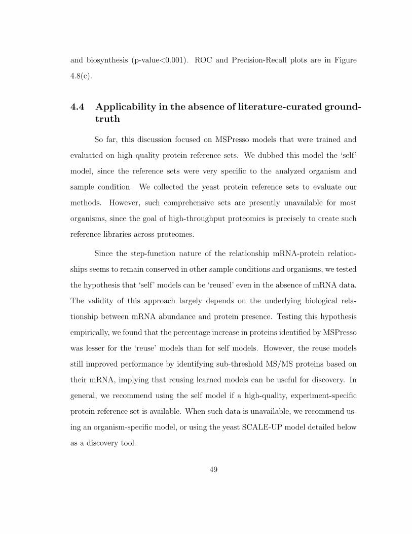
and biosynthesis (p-value<0.001). ROC and Precision-Recall plots are in Figure

4.8(c).

4.4 Applicability in the absence of literature-curated ground-truth

So far, this discussion focused on MSPresso models that were trained and

evaluated on high quality protein reference sets. We dubbed this model the ‘self’

model, since the reference sets were very specific to the analyzed organism and

sample condition. We collected the yeast protein reference sets to evaluate our

methods. However, such comprehensive sets are presently unavailable for most

organisms, since the goal of high-throughput proteomics is precisely to create such

reference libraries across proteomes.

Since the step-function nature of the relationship mRNA-protein relation-

ships seems to remain conserved in other sample conditions and organisms, we tested

the hypothesis that ‘self’ models can be ‘reused’ even in the absence of mRNA data.

The validity of this approach largely depends on the underlying biological rela-

tionship between mRNA abundance and protein presence. Testing this hypothesis

empirically, we found that the percentage increase in proteins identified by MSPresso

was lesser for the ‘reuse’ models than for self models. However, the reuse models

still improved performance by identifying sub-threshold MS/MS proteins based on

their mRNA, implying that reusing learned models can be useful for discovery. In

general, we recommend using the self model if a high-quality, experiment-specific

protein reference set is available. When such data is unavailable, we recommend us-

ing an organism-specific model, or using the yeast SCALE-UP model detailed below

as a discovery tool.

49

0

0.2

0.4

0.6

0.8

1

0 0.2 0.4 0.6 0.8 1

Tru

e P

ositi

ve R

ate

False Positive Rate


(a) E. coli

0

0.2

0.4

0.6

0.8

1

0 0.2 0.4 0.6 0.8 1

Pre

cisi

on

Recall


(b) E. coli

0

0.2

0.4

0.6

0.8

1

0 0.2 0.4 0.6 0.8 1

Tru

e P

ositi

ve R

ate

False Positive Rate


(c) Human-Daoy-ORBI

0

0.2

0.4

0.6

0.8

1

0 0.2 0.4 0.6 0.8 1

Pre

cisi

on

Recall


(d) Human-Daoy-ORBI

0

0.2

0.4

0.6

0.8

1

0 0.2 0.4 0.6 0.8 1

Tru

e P

ositi

ve R

ate

False Positive Rate


(e) Human-Daoy-LCQ

0

0.2

0.4

0.6

0.8

1

0 0.2 0.4 0.6 0.8 1

Pre

cisi

on

Recall


(f) Human-Daoy-LCQ

Figure 4.8: (a-b) MSPresso improves ROC on E. coli data from Section 3.1.2 at simi-lar precision. MSPresso improves ROC and PR performance on the HUMAN-DAOYdata from Section 3.1.3.1 analyzed on the (c-d) LTQ-Orbitrap mass spectrometer(e-f) LCQ mass spectrometer

50

4.4.1 Reusing pre-trained models

Consider a dataset which has MS/MS identification probabilities S ′ and ab-

solute mRNA abundance M ′, but no corresponding reference set. A pre-trained

P (K|S) logistic regression classifier can simply be applied to the S ′ values, since

they are probabilities.

We now describe reuse models for a pre-trained P (K|M) function. First,

we approximated P (K|M) by a simple step function from Figure 4.2, estimating

P (K|(log10M < 0.5))=0.10 and P (K|(log10M > 9))=0.90 (results not shown).

Next, we derived two scaled models: SCALE-UP scales the P (K|M) values in Fig-

ure 4.2 to a [0,1] interval, and SCALE-DOWN conservatively scales P (K|M) to half

of the original values (results not shown). The log-mRNA abundances M,M ′ were

scaled to a [0,1] interval before applying the scaled reuse models to M ′.

A SCALE-UP reuse model derived from Figure 4.2 (yeast rich medium data)

resulted in 6 to 14% ROC-AUC increase when applied to the other yeast datasets.

We also derived SCALE-UP models from the P (K|M) distributions learned on

other organisms (E. coli, human) and re-applied them to the respective organism’s

datasets. Selected results in are in the Table 4.2.

4.4.2 Evaluation using decoy proteins and random P (K|M)

Now consider the case when mRNA data is available, but there is no protein

reference set. Decoy databases were used to estimate the MS/MS null model (Section

2.4), and random P (K|M) functions to estimate the mRNA null model, but a

protein reference set was still required to learn the true P (K|M) model.

As described in Section 2.4.1, we first ran the MS/MS analysis on rich-

51

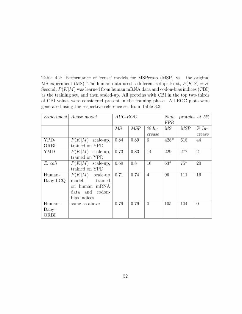
Table 4.2: Performance of ’reuse’ models for MSPresso (MSP) vs. the originalMS experiment (MS). The human data used a different setup: First, P (K|S) = S.Second, P (K|M) was learned from human mRNA data and codon-bias indices (CBI)as the training set, and then scaled-up. All proteins with CBI in the top two-thirdsof CBI values were considered present in the training phase. All ROC plots weregenerated using the respective reference set from Table 3.3

Experiment Reuse model AUC-ROC Num. proteins at 5%FPR

MS MSP % In-crease

MS MSP % In-crease

YPD-ORBI

P (K|M) scale-up,trained on YPD

0.84 0.89 6 428* 618 44

YMD P (K|M) scale-up,trained on YPD

0.73 0.83 14 229 277 21

E. coli P (K|M) scale-up,trained on YPD

0.69 0.8 16 63* 75* 20

Human-Daoy-LCQ

P (K|M) scale-upmodel, trainedon human mRNAdata and codon-bias indices

0.71 0.74 4 96 111 16

Human-Daoy-ORBI

same as above 0.79 0.79 0 105 104 0

52

0.0 0.2 0.4 0.6 0.8

05

01

00

15

02

00

25

03

00

DecoyTarget

Histograms of p-values

p-value bins

Pro

tein

co

un

ts

Figure 4.9: p-values of ProteinProphetprobabilities on decoy proteins areuniformly distributed, which suggeststhe shuffled database is a good nullmodel. However, ProteinProphet iden-tifies many shuffled proteins at highprobabilities which results in a highFalse Discovery Rate e.g. 14% FDRat 5% FPR (significance) (38 decoyproteins and 243 target proteins at5% FPR, total targets=298, total de-coys=767, 5X shuffled database)

medium yeast, matching experimental spectra against a concatenated database of

real and shuffled protein sequences. This procedure resulted in protein identification

scores S = St ∪ Sd for target and decoy proteins, letting us estimate P (K|St) using

logistic regression as before. The p-values generated from the null distribution of

ProteinProphet probabilities for decoy proteins were uniformly distributed (Figure

4.9). However the percentage of identified decoys was quite high (22%) even at high

protein probability (S > 0.8), implying that ProteinProphet has low specificity at

the protein level.

We estimate P (K) to be the same for target and decoy proteins. Since only

real proteins (targets) have mRNA abundances (Mt), we investigated several random

P (K|Md) distributions for the decoy proteins with mRNA abundance Md:

1. rand-target: randomly uniformly sampled from the target P (K|Mt) distri-

bution

2. rand-target-neg: randomly uniformly sampled from P (K|Mnt ), where Mn

t

are mRNA abundances of ‘negative instance’ target proteins i.e. proteins not

present in the protein reference set

53

3. min-target: constant at min(P (K|Mt)

4. target: set Md = Mt and P (K|Md) = P (K|Mt), same as the target distribu-

tion

5. rand-uniform: uniformly distributed in [0,1]

We ran MSPresso on the YPD-LCQ dataset in Table 3.1, using a concate-

nated database containing five times the number of decoys as targets (5X decoy,

Section 2.4.1). We generated an MSPresso probability P (K|Mt, St) for every tar-

get protein (positive instance) and P (K|Md, St) for every decoy protein (negative

instance). Since some percentage of identified target proteins could be random

hits [63], we also conservatively labeled all single-hit proteins 6 as negative instances.

It has been shown that proteins with multiple detected peptides are more likely to

be correct identifications (see Section 2.4). MSPresso achieved up to 5% ROC-AUC

increase and up to 14% more identified proteins at 5% FPR (Table 4.4.2).

4.5 Discussion

4.5.1 KD-trees for density estimation

We also implemented a density estimation method to estimate P (K|S,M)

using KD-trees [6] for space-partitioning7 [104]. KD-trees were first proposed by

Bentley in 1975, in one of the highest-cited papers in computational geometry (over

2200 citations in October 2009 as per Google Scholar). A KD-tree recursively par-

titions the space spanned by all points (s,m) in the dataset, recursively generating

equal-sized 2-way splits for each dimension. KD-trees have traditionally been used

6protein with one identified peptide and one identified spectrum7William H. Press, unpublished notes, 2007

54

Table 4.3: Evaluation without a protein reference set, on the yeast rich-mediumdataset (YPD-LCQ, Table 3.1). We use shuffled decoy databases to estimate thenull distribution. The AUC-ROC of the MS analysis was 0.93. (MSP MSPresso,MS – ProteinProphet)

AUC-ROC Number of pro-teins at 5% FPR(MS=281)

Random P (K|M) distribution MSP % Increase MSP % Increaserand-target 0.96 3.2 300 6.7min-target 0.98 5.4 320 13.7rand-target-neg 0.97 4.3 300 6.8rand-uniform 0.93 <0 270 <0target 0.96 3.2 296 5.3

for database indexing of spatial/geographical data. Gray and Moore [44] later devel-

oped a dual KD-tree data structure for efficient non-parametric density estimation.

A two-dimensional KD-tree can be used to estimate the probability P (K =

1|S = s,M = m) for each point (s,m) in the yeast dataset (Table 3.1, YPD-LCQ).

For each point (s,m) contained by a node N , P (K = 1|s,m) can be estimated as:

P (K = 1|s,m)← P (K = 1|s1 ≤ s < s2,m1 ≤ m ≤ m2) (4.4)

where U = (s1,m2) and L = (s2,m2) are the upper and lower diagonal points

of the bounding rectangle covered by node N (cuboid in higher dimensions). This

probability for every point s,m in rectangle/node N is estimated as Tn/(Tn + Fn);

where Tn and Fn are the number of positive and negative instances contained in

N . Positive (negative) instances are defined by their presence (absence) the protein

reference set D (Table 3.3, YP4).

Since the leaf nodes of KD-trees typically have one or very few points, this

makes them very efficient for K-nearest neighbor queries in low dimensional spaces,

55

but there may not be enough data at each node to give statistically significant prob-

ability estimates. Press proposed a hierarchical solution to this problem, using the

enclosing parent node (Npar) to estimate the probability for a sparse leaf node. In

a KD-tree, every node is completely contained by its parent node, and there are no

overlapping nodes by construction. The final probability estimate is a convex com-

bination of node and parent-node estimates (Equation 4.5). The process continues

recursively for each node up to the root node NR which contains all points in the

dataset.

P (K = 1|N,D) =Tn +W ∗ P (K = 1|Npar, D)

Tn + Fn +W(4.5)

W is a weighting parameter which determines the extent of dependence of the

current node on the parent node that encloses it. Press showed that this seemingly

intuitive approach of using the parent node probability had a Bayesian interpretation

[104]. Equation 4.5 can be derived assuming a binomial distribution for the posterior

probability P (K|S,M), and a Beta conjugate prior on P (K = 1). In this context,

W acts as a pseudocount, and can be expressed in terms of the parameters (α, β)

of a Beta prior distribution.

We extended the KD-tree implementation from [105] to estimate and store

the probability estimate per node, using cross-validation for training and testing

on a yeast dataset (Table 3.1:YPD-LCQ, Table 3.3:YP4). ROC and Precision-

Recall plots are shown in Figure 4.10. Performance was similar to MSPresso, with

a percentage point lower ROC-AUC and equivalent PR-AUC. Parameter W was

chosen to maximize cross-validated ROC-AUC (Figure 4.10(c), optimal W=20).

Note that this KD-tree approach does not impose any conditional independence

assumptions between the S and M variables.

56

0

0.2

0.4

0.6

0.8

1

0 0.2 0.4 0.6 0.8 1

Tru

e P

ositi

ve R

ate

False Positive Rate

MS/MS (AUC = 0.75)MSpresso (AUC = 0.89)

KD-Tree (AUC = 0.88)

(a) ROC

0

0.2

0.4

0.6

0.8

1

0 0.2 0.4 0.6 0.8 1

Pre

cisi

on

Recall

MS/MS (AUC = 0.89)MSpresso (AUC = 0.95)

KD-Tree (AUC = 0.95)

(b) Precision-Recall

0.84

0.85

0.86

0.87

0.88

0.89

0 10 20 30 40 50 60 70 80 90 100

RO

C-A

UC

Parameter W

(c) Choosing W

Figure 4.10: Using KD-tree space partitioning to estimate P (K|S,M). Performancein (a) ROC and (b) Precision-Recall is similar to MSPresso, with a percentage pointlower ROC-AUC (c) Parameter W weights the contribution of the KD-tree’s parentnode to the child node’s probability estimates. We pick W=20, since it maximizescross-validated AUC=0.88. In general, performance is not very sensitive to W.

57

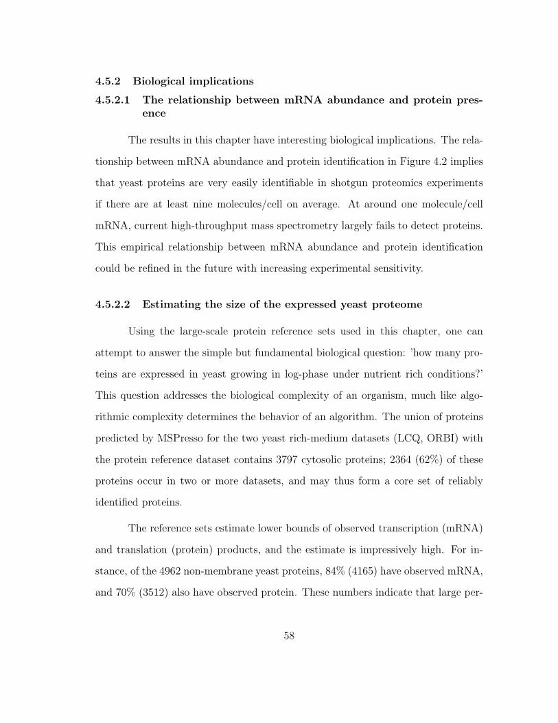
4.5.2 Biological implications

4.5.2.1 The relationship between mRNA abundance and protein pres-ence

The results in this chapter have interesting biological implications. The rela-

tionship between mRNA abundance and protein identification in Figure 4.2 implies

that yeast proteins are very easily identifiable in shotgun proteomics experiments

if there are at least nine molecules/cell on average. At around one molecule/cell

mRNA, current high-throughput mass spectrometry largely fails to detect proteins.

This empirical relationship between mRNA abundance and protein identification

could be refined in the future with increasing experimental sensitivity.

4.5.2.2 Estimating the size of the expressed yeast proteome

Using the large-scale protein reference sets used in this chapter, one can

attempt to answer the simple but fundamental biological question: ’how many pro-

teins are expressed in yeast growing in log-phase under nutrient rich conditions?’

This question addresses the biological complexity of an organism, much like algo-

rithmic complexity determines the behavior of an algorithm. The union of proteins

predicted by MSPresso for the two yeast rich-medium datasets (LCQ, ORBI) with

the protein reference dataset contains 3797 cytosolic proteins; 2364 (62%) of these

proteins occur in two or more datasets, and may thus form a core set of reliably

identified proteins.

The reference sets estimate lower bounds of observed transcription (mRNA)

and translation (protein) products, and the estimate is impressively high. For in-

stance, of the 4962 non-membrane yeast proteins, 84% (4165) have observed mRNA,

and 70% (3512) also have observed protein. These numbers indicate that large per-

58

R2 = 0.275

0.2

0.4

0.6

0.8

1.0

0.1 1 10 100 1000

S: P

rote

inPr

ophe

t pro

tein

id

entif

icat

ion

prob

abili

ty

mRNA abundance (mol/cell, log-scale base 10)

k=TP

(a)

0.2

0.4

0.6

0.8

1.0

0.1 1 10 100

S: P

rote

inPr

ophe

t pro

tein

id

entif

icat

ion

prob

abili

ty

mRNA concentration (mol/cell, log-scale, binned)

k=TN

(b)

R2 = 0.0506 0.2

0.4

0.6

0.8

1.0

0.1 1 10 100

S: P

rote

inPr

ophe

t pro

tein

id

entif

icat

ion

prob

abili

ty

mRNA abundance (mol/cell, log-scale base 10)

k=TN

(c)

0.2

0.4

0.6

0.8

1.0

0.1 1 10 100 S:

Pro

tein

Prop

het p

rote

in

iden

tific

atio

n pr

obab

ility

mRNA concentration (mol/cell, log-scale, binned)

k=TN

(d)

Figure 4.11: There is very low correlation between ProteinProphet probability (S)and mRNA abundance. In general, there is better correlation for proteins expectedto be present in the sample (R2=0.275, k=TP, proteins present in the YP4 referenceset) than for proteins not expected in the sample (R2=0.05, k=TN, proteins absentfrom YP4 reference set). The second column shows binned equivalents of the scatterplots (50 proteins per bin, total number of proteins=872)

centages of the genome are expressed even in an unperturbed unicellular eukaryote.

Interestingly, there are 282 genes for which no mRNA is observed but protein is

confidently detected. An explanation is that mRNA may exist at only very low

levels or is rapidly degraded.

4.5.2.3 Correlation between mRNA and probability of protein presence

The Figure 4.11 shows only a weak correlation between S and M given pro-

tein presence (r = 0.09 for K = 1, r = 0.01 for K = 0), which might seem surprising

given the good observed correlation between mRNA and protein abundance for con-

59

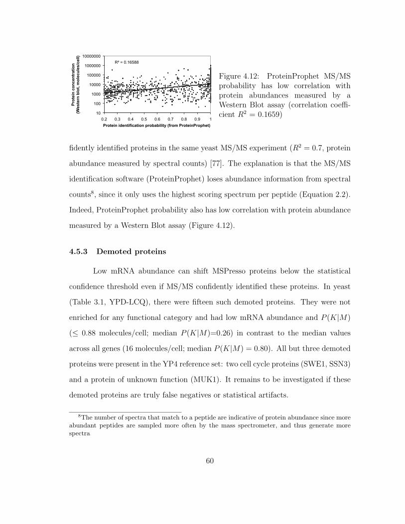
R! = 0.16588

10

100

1000

10000

100000

1000000

10000000

0.2 0.3 0.4 0.5 0.6 0.7 0.8 0.9 1

Pro

tein

co

ncen

trati

on

(W

este

rn b

lot,

mo

lecu

les/c

ell)

Protein identification probability (from ProteinProphet)

Figure 4.12: ProteinProphet MS/MSprobability has low correlation withprotein abundances measured by aWestern Blot assay (correlation coeffi-cient R2 = 0.1659)

fidently identified proteins in the same yeast MS/MS experiment (R2 = 0.7, protein

abundance measured by spectral counts) [77]. The explanation is that the MS/MS

identification software (ProteinProphet) loses abundance information from spectral

counts8, since it only uses the highest scoring spectrum per peptide (Equation 2.2).

Indeed, ProteinProphet probability also has low correlation with protein abundance

measured by a Western Blot assay (Figure 4.12).

4.5.3 Demoted proteins

Low mRNA abundance can shift MSPresso proteins below the statistical

confidence threshold even if MS/MS confidently identified these proteins. In yeast

(Table 3.1, YPD-LCQ), there were fifteen such demoted proteins. They were not

enriched for any functional category and had low mRNA abundance and P (K|M)

(≤ 0.88 molecules/cell; median P (K|M)=0.26) in contrast to the median values

across all genes (16 molecules/cell; median P (K|M) = 0.80). All but three demoted

proteins were present in the YP4 reference set: two cell cycle proteins (SWE1, SSN3)

and a protein of unknown function (MUK1). It remains to be investigated if these

demoted proteins are truly false negatives or statistical artifacts.

8The number of spectra that match to a peptide are indicative of protein abundance since moreabundant peptides are sampled more often by the mass spectrometer, and thus generate morespectra

60

4.5.4 Reliability of MS/MS protein probabilities

MSPresso estimates P (K = 1|S) instead of directly using the ProteinProphet

protein probability S. First, the ProteinProphet probability is not a conditional

probability (Equation 2.2). Second, in our experiments, S over-estimated the prob-

ability of a correct identification, especially at high probabilities (the important

region, see Figure 4.13). The ProteinProphet authors empirically showed that the

protein probability (PP) was a good estimate of P (K = 1|S). They plotted PP vs.

P (K = 1|S) estimated using a control-mix decoy database to define false identifica-

tions (Section 2.4). PP was considered to be a conservative estimate of P (K = 1|S)

if the curve was parallel and above the diagonal. We were unable to replicate these

plots using our MS/MS data and our notion of ground-truth. We observed that Pro-

teinProphet probabilities were anti-conservative at high probabilities (Figure 4.13).

As in the ProteinProphet paper, we estimated P (K = 1|S) by binning proteins into

equal-sized bins, and counting the percentage of proteins per bin that were true

identifications. We tested two definitions of ’true identification’: (a) reference set

and (b) real and decoy databases. In both cases, ProteinProphet probabilities were

anti-conservative at high probabilities. On the other hand, MSPresso probabilities

were conservative (above the diagonal, Figure 4.13).

4.6 Related Work

This chapter has focused on learning the relationship between mRNA abun-

dance and protein presence. We are not aware of any studies that systemati-

cally exploit the mRNA-protein relationship to improve protein detection in mass-

spectrometry experiments. To our knowledge, related work in this area has focused

on the relationship between mRNA and protein abundances.

61

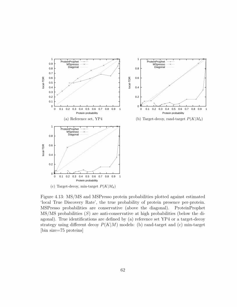
0

0.1

0.2

0.3

0.4

0.5

0.6

0.7

0.8

0.9

1

0 0.1 0.2 0.3 0.4 0.5 0.6 0.7 0.8 0.9 1

loca

l-TD

R

Protein probability

ProteinProphetMSpressoDiagonal

(a) Reference set, YP4

0

0.2

0.4

0.6

0.8

1

0 0.1 0.2 0.3 0.4 0.5 0.6 0.7 0.8 0.9 1

loca

l-TD

R

Protein probability


(b) Target-decoy, rand-target P (K|Md)

0

0.2

0.4

0.6

0.8

1

0 0.1 0.2 0.3 0.4 0.5 0.6 0.7 0.8 0.9 1

loca

l-TD

R

Protein probability


(c) Target-decoy, min-target P (K|Md)

Figure 4.13: MS/MS and MSPresso protein probabilities plotted against estimated‘local True Discovery Rate’, the true probability of protein presence per-protein.MSPresso probabilities are conservative (above the diagonal). ProteinProphetMS/MS probabilities (S) are anti-conservative at high probabilities (below the di-agonal). True identifications are defined by (a) reference set YP4 or a target-decoystrategy using different decoy P (K|M) models: (b) rand-target and (c) min-target[bin size=75 proteins]

62

4.6.1 Protein abundance vs. mRNA abundance

Initial large-scale studies to correlate mRNA and protein abundances were

motivated by the limited ability to measure protein abundances on large-scale.

Global correlation measurement is complicated due to the biological complexity

of protein creation. For instance, post-transcriptional regulation, post-translational

modifications can confound large-scale protein abundance measurement and differ-

ences in mRNA and protein degradation rates can confound large-scale correlation

measurements.

A range of correlation studies were surveyed by Greenbaum et al [45] in 2003.

Greenbaum et al also performed their own study, combining previously analyzed 2D-

gel and MudPIT9 experiments to get better estimates of protein abundance. They

found a global correlation of R2 = 0.66 with varying correlation based on cellular

location (R2=0.2 to R2=0.89). Kannan et al showed that a hierarchical Bayesian

model can be much more effective at predicting the relationship between mRNA

and protein abundance than standard linear regression approaches [57,64].

In 2007, Peng et al reported improved correlation estimates for confidently

identified proteins using spectral counts as surrogates for protein abundance (R2=0.73

in yeast and R2=0.47 in E. coli for log-scaled data). There have been very recent

important technical advances in mass spectrometers, ionization techniques and com-

putational methods that aid measurement of absolute protein abundance. There are

primarily two camps: one using spectral counts, and the other using spectral peak

intensity. A recent survey is in [135] and further discussion in Chapter 8.

9Multidimensional Protein Identification Technology: instead of separation of proteins by 2D-gel, uses liquid chromatography separation followed by mass spectrometry. In this dissertation,the term ‘MuDPIT’ is used interchangeably with ‘shotgun proteomics’

63

4.7 Software and availability

Software is available at the MSPresso website: http://marcottelab.org/

MSpresso

64

Chapter 5

Network priors from gene functional networks

5.1 Introduction

1 Sets of functionally-related proteins carry out distinct biological processes

in a cell. In initial feasibility analysis, we found that the probability of detecting

proteins whose network neighbors had been detected by MS/MS was significantly

higher than the probability of detecting proteins whose neighbors had not been de-

tected (Figure 5.1). This chapter introduces an additional stage of computational

analysis to MS/MS shotgun protein identification that exploits gene functional net-

works 2 [84] to analyze MS-identified proteins in the context of functionally-related

groups of genes.

Specifically, we work with the hypothesis that it is more likely for two func-

tionally linked proteins to be co-expressed in a sample. This suggests that if proteins

p1 and p2 are known to physically interact, be co-expressed or co-regulated across

several biological conditions, and p1 has been observed in a MS experiment, p1

should be assigned a revised identification score that depends on its own MS-based

identification score c1 as well as on the MS identification of its functional neighbor

p2, moderated by the strength of belief in the functional link between p1 and p2.

1All figures and tables are at the end of this chapter2large, sparse graph of functional dependencies between all known genes of an organism, con-

structed via probabilistic analysis of several high-throughput experiments that measure some es-timate of shared gene function

65

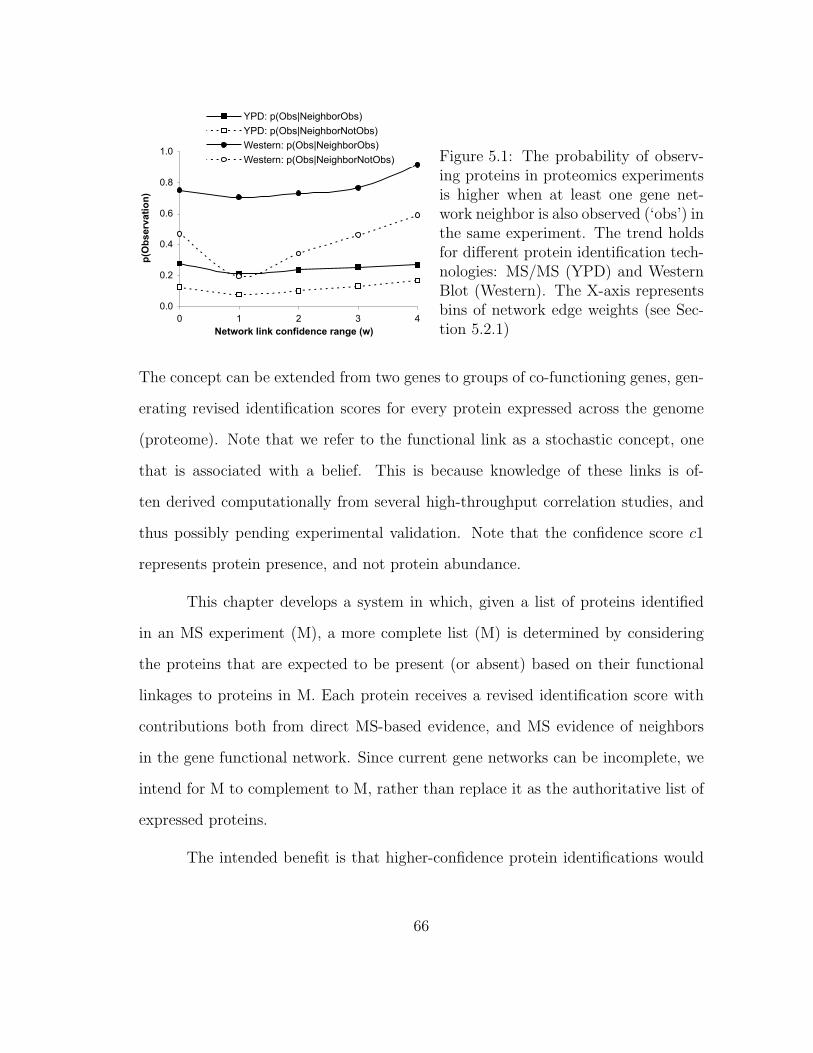
0.0

0.2

0.4

0.6

0.8

1.0

0 1 2 3 4

Network link confidence range (w)

p(O

bserv

ati

on

)

YPD: p(Obs|NeighborObs)

YPD: p(Obs|NeighborNotObs)

Western: p(Obs|NeighborObs)

Western: p(Obs|NeighborNotObs) Figure 5.1: The probability of observ-ing proteins in proteomics experimentsis higher when at least one gene net-work neighbor is also observed (‘obs’) inthe same experiment. The trend holdsfor different protein identification tech-nologies: MS/MS (YPD) and WesternBlot (Western). The X-axis representsbins of network edge weights (see Sec-tion 5.2.1)

The concept can be extended from two genes to groups of co-functioning genes, gen-

erating revised identification scores for every protein expressed across the genome

(proteome). Note that we refer to the functional link as a stochastic concept, one

that is associated with a belief. This is because knowledge of these links is of-

ten derived computationally from several high-throughput correlation studies, and

thus possibly pending experimental validation. Note that the confidence score c1

represents protein presence, and not protein abundance.

This chapter develops a system in which, given a list of proteins identified

in an MS experiment (M), a more complete list (M) is determined by considering

the proteins that are expected to be present (or absent) based on their functional

linkages to proteins in M. Each protein receives a revised identification score with

contributions both from direct MS-based evidence, and MS evidence of neighbors

in the gene functional network. Since current gene networks can be incomplete, we

intend for M to complement to M, rather than replace it as the authoritative list of

expressed proteins.

The intended benefit is that higher-confidence protein identifications would

66

reduce the workload of a biological verification step by reducing false positives and

false negatives based on the network (or mRNA) prior. For instance, Section 8.2.1

discusses our work on visualization of the revised protein list in the context of

biological pathways as a tool to aid verification of the newly identified network-

analysis based proteins.

This data integration approach has the potential to enable pathway-based

interpretation of high-throughput MS/MS experiments that are otherwise run in

isolation. For instance, it increases protein coverage in several expected active path-

ways in rich-medium yeast (Section 5.5.1) e.g. ribosomal complexes, RNA binding,

processing and degradation. In yeast growing in minimal medium, it increases the

number of proteins identified in the reductive carboxylate cycle pathway [93]. In

both cases, the newly identified proteins were expected to be present in the sample,

but were not identified with confidence by the MS analysis software, despite having

at least one peptide identified per protein.

5.2 Methods

5.2.1 MSNet algorithm

A protein identification experiment on the sample gives us probabilities of

protein presence based on MS/MS evidence for peptides of the protein (Equation

5.2). This probability is computed independently of the other proteins in the sam-

ple. Also, consider a graph G = (V,E) with |V | = N genes and weighted edges

(i, j, wij) ∈ E. The edge weight wij is proportional to the probability of a functional

link between genes i and j, the probability of the two genes participating in the same

67

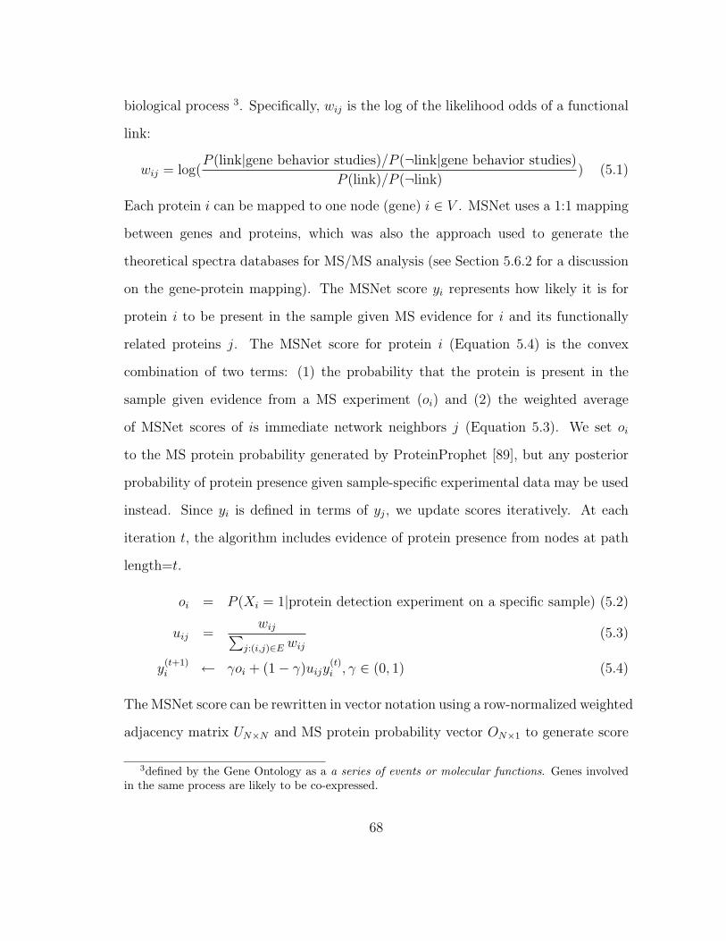
biological process 3. Specifically, wij is the log of the likelihood odds of a functional

link:

wij = log(P (link|gene behavior studies)/P (¬link|gene behavior studies)

P (link)/P (¬link)) (5.1)

Each protein i can be mapped to one node (gene) i ∈ V . MSNet uses a 1:1 mapping

between genes and proteins, which was also the approach used to generate the

theoretical spectra databases for MS/MS analysis (see Section 5.6.2 for a discussion

on the gene-protein mapping). The MSNet score yi represents how likely it is for

protein i to be present in the sample given MS evidence for i and its functionally

related proteins j. The MSNet score for protein i (Equation 5.4) is the convex

combination of two terms: (1) the probability that the protein is present in the

sample given evidence from a MS experiment (oi) and (2) the weighted average

of MSNet scores of is immediate network neighbors j (Equation 5.3). We set oi

to the MS protein probability generated by ProteinProphet [89], but any posterior

probability of protein presence given sample-specific experimental data may be used

instead. Since yi is defined in terms of yj, we update scores iteratively. At each

iteration t, the algorithm includes evidence of protein presence from nodes at path

length=t.

oi = P (Xi = 1|protein detection experiment on a specific sample) (5.2)

uij =wij∑

j:(i,j)∈E wij(5.3)

y(t+1)i ← γoi + (1− γ)uijy

(t)i , γ ∈ (0, 1) (5.4)

The MSNet score can be rewritten in vector notation using a row-normalized weighted

adjacency matrix UN×N and MS protein probability vector ON×1 to generate score

3defined by the Gene Ontology as a a series of events or molecular functions. Genes involvedin the same process are likely to be co-expressed.

68

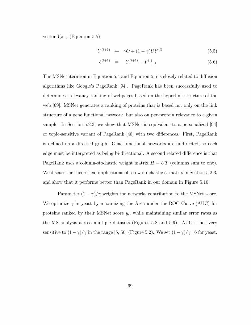
vector YN×1 (Equation 5.5).

Y (t+1) ← γO + (1− γ)UY (t) (5.5)

δ(t+1) = ‖Y (t+1) − Y (t)‖1 (5.6)

The MSNet iteration in Equation 5.4 and Equation 5.5 is closely related to diffusion

algorithms like Google’s PageRank [94]. PageRank has been successfully used to

determine a relevancy ranking of webpages based on the hyperlink structure of the

web [69]. MSNet generates a ranking of proteins that is based not only on the link

structure of a gene functional network, but also on per-protein relevance to a given

sample. In Section 5.2.3, we show that MSNet is equivalent to a personalized [94]

or topic-sensitive variant of PageRank [48] with two differences. First, PageRank

is defined on a directed graph. Gene functional networks are undirected, so each

edge must be interpreted as being bi-directional. A second related difference is that

PageRank uses a column-stochastic weight matrix H = UT (columns sum to one).

We discuss the theoretical implications of a row-stochastic U matrix in Section 5.2.3,

and show that it performs better than PageRank in our domain in Figure 5.10.

Parameter (1− γ)/γ weights the networks contribution to the MSNet score.

We optimize γ in yeast by maximizing the Area under the ROC Curve (AUC) for

proteins ranked by their MSNet score yi, while maintaining similar error rates as

the MS analysis across multiple datasets (Figures 5.8 and 5.9). AUC is not very

sensitive to (1−γ)/γ in the range [5, 50] (Figure 5.2). We set (1−γ)/γ=6 for yeast.

69

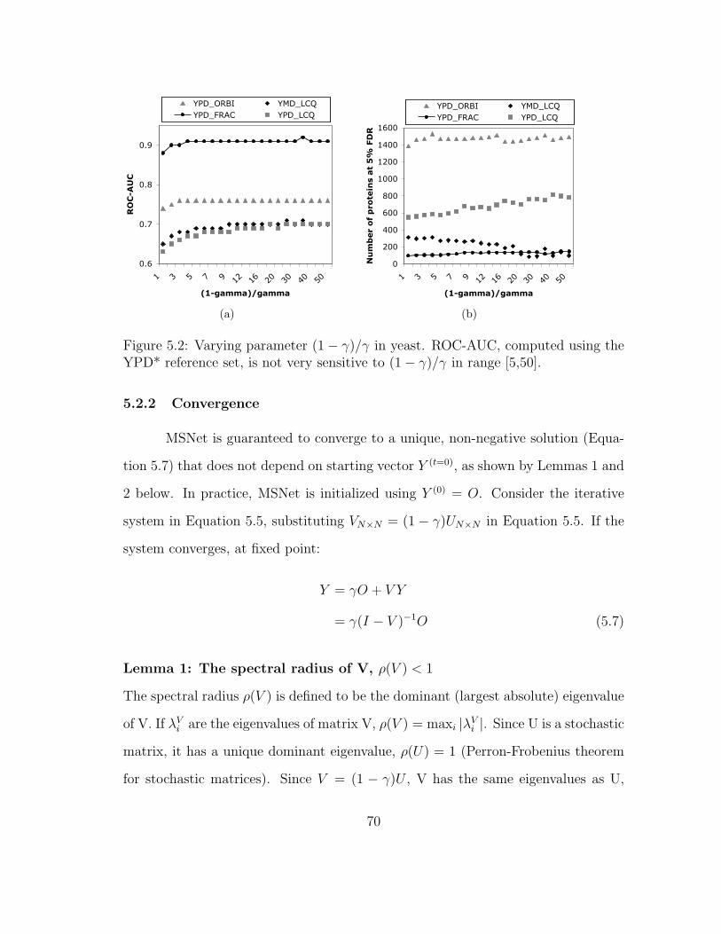
0.6

0.7

0.8

0.9

1 3 5 7 9 12 16 20 30 40 50

(1-gamma)/gamma

ROC-AUC

YPD_ORBI YMD_LCQ

YPD_FRAC YPD_LCQ

(a)

0

200

400

600

800

1000

1200

1400

1600

1 3 5 7 9 12 16 20 30 40 50

(1-gamma)/gamma

Nu

mb

er o

f p

ro

tein

s a

t 5

% F

DR

YPD_ORBI YMD_LCQ

YPD_FRAC YPD_LCQ

(b)

Figure 5.2: Varying parameter (1− γ)/γ in yeast. ROC-AUC, computed using theYPD* reference set, is not very sensitive to (1− γ)/γ in range [5,50].

5.2.2 Convergence

MSNet is guaranteed to converge to a unique, non-negative solution (Equa-

tion 5.7) that does not depend on starting vector Y (t=0), as shown by Lemmas 1 and

2 below. In practice, MSNet is initialized using Y (0) = O. Consider the iterative

system in Equation 5.5, substituting VN×N = (1 − γ)UN×N in Equation 5.5. If the

system converges, at fixed point:

Y = γO + V Y

= γ(I − V )−1O (5.7)

Lemma 1: The spectral radius of V, ρ(V ) < 1

The spectral radius ρ(V ) is defined to be the dominant (largest absolute) eigenvalue

of V. If λVi are the eigenvalues of matrix V, ρ(V ) = maxi |λVi |. Since U is a stochastic

matrix, it has a unique dominant eigenvalue, ρ(U) = 1 (Perron-Frobenius theorem

for stochastic matrices). Since V = (1 − γ)U , V has the same eigenvalues as U,

70

multiplied by (1 − γ). Therefore ρ(V ) = (1 − γ) < 1, since by definition γ ∈ (0, 1)

(Equation 5.4).

Lemma 2: (I − V )−1 exists, and is non-negative

To show this, we show that (I − V ) is an M-matrix. A matrix of the form A =

sI − B, s > 0, B ≥ 0 is an M-matrix if s ≥ ρ(B), the spectral radius of B ( [7],

p.133). (I − V ) is an M-matrix (s=1, V > 0) since 1 > ρ(V ) by Lemma 1. Since

M-matrices are inverse positive, (I − V )−1 > 0 ( [7], p.137).

In practice, convergence of the iterations is measured by the L1 norm between

the Y vectors at the tth and (t-1)th iterations (Equation 5.6). The system is said to

have converged when the L1 norm remains less than a defined error tolerance εY ,

for a defined number of consecutive iterations T . Under these conditions, MSNet

converges within 10−6 tolerance in tens of iterations.

5.2.3 Relationship of MSNet to Google’s PageRank

We first briefly describe the PageRank [94] algorithm in Section 5.2.3.1. We

then show equivalence of a personalized or topic-sensitive variant of PageRank to

MSNet, with two differences as discussed in Section 5.2.3.3.

5.2.3.1 PageRank

PageRank computes a relevance ranking for all webpages in a directed web-

page graph G=(V,E). Each webpage is a node in the graph (|V | = N). There is

an edge eij ∈ E if page j links to page i, denoted as ∃(j → i). PageRank, a rank

71

vector RN×1, is the solution to the iteration:

R(t+1) = GR(t), ‖R‖(t)1 = 1 (5.8)

G = αV ET + (1− α)(H +D) (5.9)

VN×1 = [1/N ]N×1 (5.10)

Hij =

{1/Loj ∃(j → i) and Loj = |k| s.t. ∃(j → k),∀k ∈ V0 otherwise

(5.11)

Dij =

{Vj ∀j, if |Loi | = 0

0 otherwise(5.12)

EN×1 = [1]N×1 (5.13)

where HN×N is a square, column-stochastic matrix corresponding to the web

graph, such that hij = 1/Loj if there is a link from page j to page i where Loj is the

total number of out-links from page j. The PageRank paper calls V a ’teleportation

vector’; Vj represents the probability that a web-surfer will directly jump to page j

from any another page in the web, instead of following a chain of hyperlinks to reach

j. D is an adjustment to incorporate dangling nodes i, which are nodes with no

outlinks (|Loi | = 0). It adds a pseudo-link of weight Vj = 1/N from a dangling node

i to every node j ∈ V in the graph i.e. Dij represents the probability of teleporting

from node i to node j.

An intuitive explanation for PageRank appears in the original paper, ex-

plained with the aid of a Random Surfer model [94]. Under this model, the normal-

ized PageRank vector defines a probability distribution over the web. At conver-

gence, the PageRank of page i is the probability that a surfer will ultimately land

at a page i, if his surfing behavior is modeled by two terms

1. With probability α, the surfer directly jumps from the current page i to some

72

page k instead of clicking on a hyperlink in i (k is chosen with probability Vk)

2. With probability (1−α), the surfer follows a hyperlink from the current page

i to a linked page j

A theoretical explanation for PageRank stems from Markov chain theory. We

briefly state the requirement for convergence here, and refer the reader to [69] for

details. In short, the PageRank iterations are equivalent to a power-method, and

converge to the dominant eigenvector of matrix G (Equation 5.9). PageRank will

converge to a unique solution if G is a stochastic and irreducible. The convergence is

independent of starting point if G is also aperiodic. The PageRank authors carefully

constructed G to satisfy these properties, by adding components D and V to H. Thus,

G’s dominant eigenvector XG exists, is non-negative, and at convergence Ri = XGi .

5.2.3.2 Topic-sensitive or Personalized PageRank

Note that PageRank as defined in Equation 5.8 does not include informa-

tion about a page’s content similarity to a search query. It only uses hyperlink-

information to rank pages. The authors suggest a modification to PageRank that

factors in similarity to the search query, by using a personalization vector V’ that

is non-uniform e.g. V’[i] is the probability that page i is relevant to the search

query [94]. This implies that PageRank must be recomputed with a new V’ vector

for every query. This approach is ideal in theory but impossible to compute in prac-

tice due to the scale of Google’s hyperlink matrix: it contains 1012 unique web pages

as of 2008 [1]. For our application in protein networks, this approach is feasible as

discussed below.

Haveliwala [48] proposed Topic-Sensitive PageRank (TSPR) as an efficient

73

alternative for Google. TSPR first classifies all pages into a predefined number of

topics (T), and generates |T | different PageRank vectors, TSPRt, t ∈ [1 . . . T ]. At

run-time, the final PageRank vector is a weighted average of the |T | Topic-Sensitive

PageRank vectors, with each TSPRt weighted by the probability that the query is

related to topic t.

MSNet uses the former simple approach, replacing the uniform vector V by

non-uniform mass-spectrometry vector O. Oi represents the probability that protein

i is ’relevant’ to the sample (present in the sample). We recompute a new ranking of

proteins for every sample (query), biasing (personalizing) the MSNet score (PageR-

ank) by the proteins more likely to be present in the sample based on MS/MS data.

Recomputing a new rank for each sample is quite feasible using the very sparse

protein networks (103 − 105 nodes, 99.94% sparse).

5.2.3.3 Relationship

MSNet’s Equation 5.5 is equivalent to Equations 5.8-5.9 by setting Y ≡ R,

O ≡ V , U ≡ HT . D = 0 since there are no dangling nodes in an undirected

graph: each edge is bi-directional, so all nodes have in-links and out-links. The

only difference then is that MSNet uses a row-stochastic matrix U, and PageRank

uses a column-stochastic matrix H (H = UT ). PageRank uses normalized vectors

‖R(t)‖1 = 1, ‖V ‖1 = 1 (Equation 5.8). The normalization of R does not change

the relative ranking, and avoids underflow. In fact, the PageRank iteration can be

written as a power-method on matrix G since R, V and H are column-stochastic

(Equation 5.8).

In Figure 5.10, we show that a row-stochastic U matrix performs much better

in our domain. This improved performance can be explained as follows. The effect

74

of column-stochastic H (∑

j Hij = 1) is that if page A links to B (∃(A→ B), HBA =

1/|LoA|), A’s contribution to B is normalized by the number of outlinks from A.

Intuitively, this implies that pages that indiscriminately link to thousands of pages

are to be trusted lesser than pages with smaller number of out-links [69]. In the

undirected gene network, we do not necessarily want to down-weight the contribution

of nodes with many neighbors. For example, consider gene A which belongs to a

large inter-connected protein complex, and is known to be present in a sample.

Also assume that A and B are linked in the gene network. The likelihood that B

is also present in the sample depends only on the strength of the link wAB, and

not on the size of A’s neighborhood |LA|. In fact, we suspect that wAB already

includes information about LA, since it is likely that large protein complexes will be

inter-connected with high edge-weights e.g. ribosomal complexes [71].

Instead, we normalize A’s contribution to B by the neighborhood of B, |LB|,

resulting in a row-stochastic matrix U (∑

i Uij = 1). This approach has two simple

interpretations. First, at each iteration, B’s score is most influenced by the score of

the node to which it has the strongest functional link. Second, the neighborhood’s

contribution to B at each iteration is simply the weighted average of B’s neighbors’

MSNet scores. It is important to note that the different normalization implies that

MSNet, unlike PageRank, is not a random walk (see below). Regardless, we have

shown that MSNet has a unique solution vector that is the inverse of an M-matrix

multipled by the mass-spectrometry protein probability vector O (Section 5.2.2).

Normalizing ‖O‖1 = 1 and ‖Y (t)‖1 = 1 at each iteration, we can rewrite

75

MSNet’s Equation 5.5 exactly in the form of PageRank’s Equations 5.8-5.9:

Y (t+1) = G′Y (t), ‖Y ‖(t)

1 = 1 (5.14)

G′= αOET + (1− α)U (5.15)

However, unlike PageRank, MSNet is not a random-walk since G′

is not stochastic.

PageRank’s matrix G is stochastic because it is the convex combination of two

column-stochastic matrices: V ET and (H + D) (Equation 5.8). In contrast, gene

matrix G′

is the convex combination of column-stochastic O′ET and row-stochastic

U. Finally, PageRank can also be expressed the solution to a linear system, with

‖R‖1 = 1 [69]:

R = α(I − (1− α)(H +D))−1V (5.16)

5.3 Datasets

MS/MS data: MSNet is effective in yeast across different experimental

conditions and mass spectrometers, and also effective on human samples. The pro-

teomics are datasets described in Section 3.1.

Gene networks: MSNet uses the yeast gene functional network created by

Lee et al [71] spans >95% of the yeast genes. The weight wij of an edge between

two genes i and j is defined as the log of the likelihood odds ratio that there exists a

link, and is determined by Bayesian integration of thousands of diverse experiments

that estimate functional association e.g. mRNA co-expression, phylogenetic profiles,

protein interaction experiments and co-citation in published literature. A similarly

constructed human gene network was used for human samples in this chapter (Lee

and Marcotte, manuscript in preparation).

76

5.4 Evaluation Methodology

For a given mass spectrometry experiment and gene functional network, the

MSNet protein identification score is computed using Equation 5.4 for every protein

on a genome-wide scale. To test robustness to missing network links, the average

MSNet score is reported across ten runs of ten fold cross-validation. Functional

analysis of yeast proteins was conducted using SGD [88], FunSpec [114] and Fun-

cAssociate [8], applying Bonferroni corrections.

Protein universe MSNet considered the entire yeast genome except for

proteins annotated as ‘dubious’, since these proteins were not considered in the yeast

network [70, 71]. Proteins with no neighbors in the network (network singletons)

were also included in the iteration (Equation 5.4). Of total 294 singleton genes in

YeastNet2 network, only 101 genes that had at least one peptide identified in MS/MS

experiment were included in the MSNet computation. These network singletons are

proteins with no statistically significant observed associations with any other gene,

in the thousands of experiments that were used to create the yeast network. It

is likely that these proteins are not present in a sample, and thus might be false

proteomics identifications. For this reason, singleton genes were included into our

analyses to see if MSNet would correctly demote singletons. Indeed, MSNet did

better than the MS/MS experiment at classifying singletons as negative instances

(Section 5.5.1).

MS probability oi Only proteins with at least one identified peptide were

included in the ROC/PR evaluation. The lowest non-zero probability reported by

ProteinProphet is always oi = 0.2 (TPP, version 4.0), and ProteinProphet scales

all probabilities < 0.2 to zero. These proteins generally either had only a single

77

identified peptide, or contained peptides identified with low probability. Since these

‘doubtful’ proteins did have some peptides identified, they were included in the

MSNet computation to investigate if they could be rescued based on network evi-

dence. Doubtful proteins in the yeast and human datasets in Table 3.1 were given

random low MS/MS identification probabilities oi ∈ [0, 0.2) before being fed into

the MSNet iteration.

A 5% False Discovery Rate (FDR) was employed to determine a high-confidence

list of proteins with MSNet scores. FDR was estimated using two approaches: (a)

using a protein reference set as ground-truth (b) generating true and false (null)

score distributions independent of ground truth based on label-shuffled networks.

5.4.1 Evaluation against a protein reference set

A protein was labeled as a true instance (T) if it was present in the reference

set, and as a false instance (F) otherwise. FDR at score threshold s was estimated

as FDRref = Fs/(Ts + Fs), the percentage of all instances with score ≥ s that

were false identifications. ROC and Precision-Recall curves were plotted using the

reference set as ground-truth.

5.4.2 Evaluation independent of a protein reference set

When protein reference sets are unavailable, it is standard to compute er-

ror estimates by generating a null distribution of scores from the null hypotheses

(Section 2.4.1). MSNet uses a random error model for the network’s contribution,

dubbed label-shuffling, that is similar to randomization or permutation tests used in

statistical hypothesis testing. For a given dataset, null MSNet scores were generated

by running MSNet on a network where the labels on the nodes (protein names) were

78

shuffled, such that proteins maintained features such as the MS/MS protein identi-

fication score, but had a different set of network neighbors. Label-shuffling destroys

any biological gene-gene association signal, while maintaining network topology (e.g.

node degree and edge distribution). Label-shuffling was repeated multiple times to

create several ‘null networks’, and MSNet was run on each of them. The resulting

protein scores were pooled into a null score distribution. The true score distribution

was generated by running MSNet on the original network. Density distributions for

null and true scores are shown in Figure 5.11 for yeast data and Figure 5.11(e) for

human data. FDR was estimated as FDRshuff = Ns/Ts, where Ns is the area under

the null distribution for scores ≥ s and Ts is the area under the true distribution for

scores ≥ s. In this chapter, FDR refers to FDRshuff unless stated otherwise. Note

that the null distributions can be used to compute any other desired error estimate

(e.g. p-value, q-value).

5.5 Results

Incorporating functional association information substantially boosted cor-

rect identification of proteins in shotgun proteomics experiments, across a range of

sample conditions and mass spectrometers. ROC and Precision-Recall plots were

generated for yeast datasets and the Human-293T dataset in Table 3.1. The number

of proteins identified by MSNet at 5% FDR were compared to the MS/MS experi-

ment at its 5% FDR. ProteinProphet computes FDR at score threshold s directly

from its protein probabilities, as one minus the average protein probability at score

threshold ≥ s [89].

MSNet consistently increased the number of proteins identified at 5% FDRshuff

by 8-29% across yeast experiments (Table 5.3). At least 94% of MSNet proteins were

79

validated either by presence in the reference set, or by confident identification in the

MS/MS experiment (Figure 5.3). When applied to the human proteome using a

human functional gene network, MSNet reported up to 37% more proteins than the

MS/MS analysis.

When evaluated using protein reference sets for our yeast experiments. MSNet

increased the number of identifications at 5% FDRref by 12-100% across datasets

and increased ROC-AUC by up to 24% (Table 5.1). MSNet is also applicable to

data generated from different MS/MS software analysis pipelines (Section 5.5.5).

These results are described in detail below.

5.5.1 Yeast grown in rich medium

MSNet reported 1835 identifications at 5% FDR in YPD-ORBI data, a 29%

increase over the MS/MS experiment. 92% of these proteins were present in the

reference set and a further 4% were previously identified in the MS/MS experiment

(Figure 5.3). 460 MSNet proteins had not previously been identified in the MS/MS

experiment (rescued proteins). They were enriched for ribosome or translation-

associated functions when compared against a background of the whole genome,

and for proteins of unknown function compared to a background of MSNet 5%

FDR proteins (p-value<0.001). Eighty-five percent of the 460 new identifications

were present in the reference set. There were no obvious false-positives from a

protein function analysis since the remaining fifteen percent were not enriched for

any function category.

In a ROC plot (Figure 5.4(a)), MSNet identified more true instances (proteins

present in the reference set) than the MS/MS experiment over a range of False

Positive Rates. Similarly, in a Precision-Recall plot (Figure 5.4(b)) MSNet identified

80

more true instances over a range of FDRs (1-Precision), e.g. identifying 12% more

proteins at 5% FDRref (Table 5.1). MSNet also resulted in a 10% increase in ROC

AUC, i.e. MSNet is 10% more likely than MS/MS analysis to rank a randomly

chosen true instance higher than a randomly chosen negative instance.

MSNet improved performance even when the MS/MS experiment was lim-

ited by instrument resolution, as we observed on the same sample re-analyzed on

a low-resolution mass spectrometer (Table 3.1, YPD-LCQ). MSNet reported 8%

more proteins than the MS/MS experiment and increased AUC by 24% (Table 5.1,

Figure 5.6). The new MSNet identifications were enriched for ribosomal proteins

(p-value<0.001).

Typical example of rescued proteins: Figure 5.5 illustrates two proteins

that were rescued by MSNet at 5%FDR with their immediate neighbors in the

functional network. ARC40 is an essential subunit of the ARP2/3 complex, and

RPS29B is a member of the 40S ribosomal complex. Both proteins had at least

one peptide identified in the MS/MS experiment, but their MS/MS protein scores

fell below the error threshold of the MS/MS software, and they were not identified

with confidence. Both proteins have functions appropriate for yeast growing in rich

medium, and have previously been identified with high confidence in the YPD*

reference set. Moreover, deletion of either gene causes notable growth defects [41];

strongly supporting their expression in the sample. MSNet effectively rescues both

proteins and gives them higher scores, based on the their MS/MS evidence and their

functional associations to other proteins that were confidently identified in the MS

analysis. In general, MSNet also improved protein recall in several active pathways

in rich-medium yeast e.g. glycolysis/gluconeogenesis, fatty acid metabolism, RNA

biosynthesis, amino-acid biosynthesis and degradation [28] (EASE-value=0.05).

81

MSNet demotes singleton proteins: The MSNet score for network sin-

gletons is only computed using the first γoi term in MSNet Equation 5.4, since the

second summation network-based term is zero. As a result, MSNet scores for sin-

gleton proteins were considerably lower and singleton proteins were demoted with

respect to other non-singletons. This is the correct behavior, since singleton proteins

tend to be absent from the YPD* protein reference set. When we included network

singletons into the MSNet analysis, MSNet’s ROC-AUC increases from 0.75 to 0.76

as tabulated in Table 5.2). We observed similar behavior in other yeast experiments.

Running MSNet without MS/MS data: MSNet can be run without

using MS/MS data to evaluate the extent of the network’s contribution to a protein’s

MSNet score. In this network-only mode, all proteins were given uniform MS/MS

protein probability. We expected both ProteinProphet and MSNet ROC-AUC to be

0.5, since the MSNet score yi = oi when oi = constant,∀i (Equation 5.4). However,

the network contributed 5% extra AUC even with no MS/MS evidence. The increase

can be attributed to singleton proteins, which are demoted by MSNet (yi = γoi, γ <

1). The demotion is supported by the reference set (higher than random AUC).

Note that in the presence of MS/MS evidence, the singleton effect on AUC is less

pronounced (with singletons AUC=0.76, without singletons AUC=0.75). Results

are in Table 5.2.

5.5.2 Yeast grown in minimal medium

MSNet should be informative across sample conditions, since the gene net-

work was constructed by integrating diverse biological experiments across sample-

conditions. Indeed, when applied to yeast grown in minimal medium (Table 3.1,

YMD-LCQ), MSNet identified 9% more proteins at 5% FDR (Table 5.3). The new

82

MSNet identifications were enriched for ribosomal proteins (p-value<0.001) as in the

rich-medium yeast experiment, but also for proteins of small molecule biosynthesis

(p-value<0.001) e.g. carboxylic acid, amine or folate metabolism, which is expected

for growth in minimal medium. MSNet increased AUC by 17% when evaluated

against the YMD* reference set (Table 5.1, Figure 5.6).

5.5.3 Yeast polysomal fraction

MSNet’s best application scenario is on smaller, focused protein preparations

e.g. on a polysomal fraction of yeast grown in rich medium, fractionated on a

sucrose density gradient (Table 3.1, YPD-LCQ-Fraction). Proteins in this sample

were restricted to those co-fractionating with 80S ribosomes and were expected to

be associated with ribosomal and translation functions.

MSNet identified 16% more proteins at 5% FDR than the MS/MS experiment

(Table 5.3). 94% of MSNet identifications were validated, either by presence in the

fractionation reference set or by previous identification in the MS/MS experiment

(Figure 5.3). In a function analysis, all but three new MSNet proteins were found

to be associated with the ribosome, ribosomal functions or translation4. MSNet

increased AUC by 17% when evaluated against the fractionation protein reference

set (Table 5.1). ROC and Precision-Recall curves are plotted in Figure 5.6.

4The three proteins might represent false positives: inosine monophosphate dehydrogenaseIMD2 which catalyzes the first step of GMP biosynthesis; ADK2, a mitochondrial adenylate kinasewhich catalyzes the reversible synthesis of GTP and AMP from GDP and ADP; and FLC1, aputative FAD transporter [88]

83

5.5.4 Human samples

MSNet is equally applicable to higher organisms as demonstrated by its ap-

plication to human HEK293T kidney cells analyzed on a high-resolution mass spec-

trometer (Table 3.1, Human-293T) using a human gene functional network (Lee and

Marcotte, in preparation). To test MSNet in a more complex scenario than single-

celled yeast, we considered the 18514 protein-coding genes present in the human

functional network. MSNet reported up to 40% increase in the number of identified

proteins at 5% FDR 5.3 with parameter (1 − γ)/γ varying in [6,10]. As in yeast

(Section 5.2), this parameter can be optimized as reference sets for human data

become available. The new 5% FDR MSNet proteins were not enriched for any

functional category.

5.5.5 Performance on different MS/MS pipelines

The results so far were generated using BioWorks 3.3.1 for spectral match-

ing and TPP (version 4.0) for peptide and protein identification. MSNet is also

applicable when different software pipelines are used.

There are several implementation issues that interfere with systematic testing

and comparison of different MS pipelines. First, there is currently only one pub-

lished, freely available analysis pipeline that generates protein-level probabilities and

FDRs i.e. the Trans-Proteomic Pipeline (TPP) used in this dissertation. Second,

a systematic comparison is non-trivial since each pipeline makes different statisti-

cal assumptions and the hypotheses are not independent. Third, any consolidation

effort entails significant software development time to accommodate different data

formats across pipelines [107]. Nonetheless, we tested three additional pipelines:

84

1. X!Tandem5 for spectral matching and TPP (v4.1.1) for protein identification

2. CRUX for spectral matching and Percolator for peptide identification6

3. average of protein probabilities from the above pipelines

Since Percolator does not generate protein probabilities, we computed a protein

probability based on TPP’s ProteinProphet (Equation 2.2, [89]) using Percolator’s

peptide probabilities as input. We dub this protein score PPC for ProteinProphet-

Clone. MSNet showed comparable performance improvements across pipelines, with

10-12% higher AUC, and 7-12% more proteins at 5% FDR than the original analysis

(Table 5.4, Figure 5.7). The extent of improvement from MSNet is lesser when the

MS/MS analysis is more accurate, which per expectation since the expected protein

content of the sample is constant.

Since Percolator uses a stringent 1% q-value peptide cutoff, the protein prob-

abilities generated by PPC are skewed conservatively: they are either zero or very

confident [0.9,1]. This does not leave much room for MSNet improvement. However,

there are proteins with peptides identified that all fall below the Percolator thresh-

old. Let us call this set of proteins P . We tested two versions of Percolator-PPC:

Percolator-PPC(1) excludes P from MSNet computation, and there is no improve-

ment at 5% FDRref . Percolator-PPC(2) includes P in the MSNet computation.

MSNet reports 7% more identifications on this larger input set at 5%ref supporting

our initial observation that the Percolator q-value threshold might be too conserva-

tive (Table 5.4).

5X!Tandem version 2008.12.01.1 [19]6CRUX version 1.20, [97], Percolator version 1.11 [52])

85

5.6 Discussion

Our methodology places MS/MS experiments in a larger biological frame-

work, where proteins expressed in a given cellular state may be readily analyzed

in the context of their functionally related neighbors. MSNet may be viewed as a

quantitative complement to graphical tools that map omics experiment results onto

known functional pathways [28,95].

5.6.1 Demoted proteins

MSNet improves protein identification by both increasing the number of true

identifications and reducing false identifications. Since MSNet produces a revised

ranking of MS-identified proteins, some proteins can receive lower ranks than in the

MS/MS analysis and fall below MSNets 5% FDR threshold, despite satisfying the

MS/MS 5% FDR threshold. There is some evidence that these demoted proteins

might be false positive MS/MS identifications: in yeast, the percentage of demoted

proteins that can be validated by presence in the reference set is much smaller than

the percentage of new MSNet proteins that can be validated similarly (Table 5.3).

In human, all demoted proteins were network singletons i.e. they had no network

neighbors. We list the number of demoted proteins for all experiments, as well as

the union of MS and MSNet identifications in Table 5.3.

5.6.2 Gene to protein mapping

We use the term gene product to signify any of the proteins that map to one

gene. We have so far implicitly assumed a 1:1 correspondence between genes in the

network and proteins in the sample. The gene-protein mapping is far more complex

in human than in yeast, due to ubiquitous protein isoforms. The size of the human

86

genome is surprisingly small, approximately ∼22,000 genes, in comparison to its

functional complexity. The difference is currently attributed to protein isoforms;

alternate splicing can produce different gene products from a single gene.

The MSNet protein universe consists of the protein sequence database used

during peptide identification by database lookup (Section 2.2). A widely-used sim-

plification that to ensure 1:1 gene-protein mapping is to only populate the protein

sequence database with the longest possible protein sequence per gene transcript.

The MS/MS datasets in this dissertation follow this approach.

5.7 Related work

Gene network priors have been widely used in protein function prediction.

Sharan et al published a comprehensive survey of network-based methods for pre-

diction of protein function [123], ranging from neighbor counting to random field

models. This section discusses some representative methods. Chapter 6 addresses

the network-based recommendation problem as an inference problem on graphical

models, and compares performance of MSNet to other Markov Random Field mod-

els.

Deng et al modeled the gene functional network as a Markov network, pre-

dicting a gene’s function based on the functions of its neighbors [27]. Their model is

a pairwise Markov Random Field that predicts if a gene has a given function, model-

ing a Bernoulli RV for every gene and every function. Inference via Gibbs sampling

is performed separately for every function of interest. Parameters of the model are

estimated using a quasi-likelihood approach, by performing logistic regression using

genes with known function as ground-truth for training.

87

Similarly [140] integrated KEGG pathways [93] into differential gene expres-

sion studies using an MRF approach. [139] adopted a different approach to the

problem. Instead of modeling each gene as a node in a MRF, they use a spatially

correlated mixture model [35]. A spatially correlated mixture model differs from a

standard mixture model in that it uses element-specific prior probabilities (mixing

weights for the mixtures). Wei and Pan estimate a prior probability of every gene (i)

belonging to every mixture component (j) as πij. The πij’s are estimated from the

corresponding conditional probabilities of nodes i in the jth Gaussian random field

derived from the gene functional network (Gaussian conditional auto-regression [9]).

Their spatially correlated mixture model delivered higher ROC-AUC than standard

mixture model clustering.

Very recently, Li et al developed a method with the same goal as our study:

utilize network relationships to improve protein identification [73]. They demon-

strate good performance (8-23% increase in identifications), but do not directly

compare performance with MSNet. A direct comparison is hard since CEA is demon-

strated on completely different gene networks and mass spectrometry datasets from

those used in this dissertation, but we discuss the details here. The method, called

Clique Enrichment Approach (CEA) is based on the assumption that cliques of

proteins tend to have similar properties (empirically demonstrated in the paper).

MSNet differs from CEA in the fundamental assumptions of the two meth-

ods. MSNet does not require fully-connected subgraphs (cliques), and can boost

a protein’s identification if it is connected to sufficient confident proteins. At the

same time, MSNet will implicitly boost proteins in cliques, as long as the clique has

enough confident proteins. As stated in the CEA paper, a drawback of a clique-

based approach is that not all biological processes are represented by cliques e.g.

88

signal transduction pathways. MSNet also uses information from proteins greater

than one edge away. The influence of such proteins decays per iteration based on

path length (Equation 5.4). Secondly, CEA uses a binary classification of proteins:

confident and non-confident. MSNet does not employ hard class labels, but instead

uses the probabilities of protein identification derived from the MS experiment.

The CEA methodology is summarized here for completeness: first, each

gene in the network is labeled as being a confident or non-confident identification

based on mass spectrometry analysis. Next, a graph-theoretic maximal clique find-

ing algorithm enumerates the maximal cliques in the network graph. The cliques

are ranked based on enrichment for confidently identified proteins (exact Fisher

test/hypergeometric distribution). All non-confident proteins in a clique c that

passes an enrichment score threshold are re-labeled as confident identifications.

Other non-confident identifications are discarded. CEA error rates are computed

using random networks including the label-shuffling approach used in MSNet (Sec-

tion 5.4.2), and Erdos-Renyi models [33], which do not preserve graph properties

such as clustering coefficient and node degree. The authors compare CEA to two

other network-assisted prediction approaches which have previously been applied to

protein function prediction. The first is a neighbor counting model, where the class

of a node is inferred from the class of its neighbors. The second is a global method

that uses a Hopfield network model [59], which is a special case of the Ising model,

and thus a special case of random field models. We compare performance of MSNet

to a Markov Random Field model in Chapter 6.

89

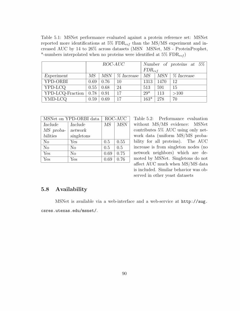
Table 5.1: MSNet performance evaluated against a protein reference set: MSNetreported more identifications at 5% FDRref than the MS/MS experiment and in-creased AUC by 14 to 26% across datasets (MSN MSNet, MS - ProteinProphet,*-numbers interpolated when no proteins were identified at 5% FDRref )

ROC-AUC Number of proteins at 5%FDRref

Experiment MS MSN % Increase MS MSN % IncreaseYPD-ORBI 0.69 0.76 10 1313 1470 12YPD-LCQ 0.55 0.68 24 513 591 15YPD-LCQ-Fraction 0.78 0.91 17 29* 113 >100YMD-LCQ 0.59 0.69 17 163* 278 70

MSNet on YPD-ORBI data ROC-AUCIncludeMS proba-bilities

Includenetworksingletons

MS MSN

No Yes 0.5 0.55No No 0.5 0.5Yes No 0.69 0.75Yes Yes 0.69 0.76

Table 5.2: Performance evaluationwithout MS/MS evidence: MSNetcontributes 5% AUC using only net-work data (uniform MS/MS proba-bility for all proteins). The AUCincrease is from singleton nodes (nonetwork neighbors) which are de-moted by MSNet. Singletons do notaffect AUC much when MS/MS datais included. Similar behavior was ob-served in other yeast datasets

5.8 Availability

MSNet is available via a web-interface and a web-service at http://aug.

csres.utexas.edu/msnet/.

90

Tab

le5.

3:P

erfo

rman

ceev

aluat

ion

wit

hou

ta

pro

tein

refe

rence

set:

Pro

tein

sid

enti

fied

only

by

MSN

et,

only

by

MS/M

San

alysi

san

dunio

nof

pro

tein

sid

enti

fied

by

bot

hM

SN

etan

dM

S/M

S.

(A)

Per

centa

geof

MSN

etid

enti

fi-

cati

ons

that

can

be

validat

edby

pre

sence

inth

ere

fere

nce

set

(in

refs

et),

orby

pre

vio

us

iden

tifica

tion

by

MS/M

S(M

S).

Not

eth

atre

fere

nce

sets

for

YP

D-L

CQ

-Fra

ctio

nan

dY

MD

-LC

Qar

enot

asco

mple

teas

the

refe

rence

set

for

YP

D,

whic

hm

ight

expla

inw

hy

the

%va

lidat

ednum

ber

sfo

rth

ese

dat

aset

sar

em

uch

low

erth

anfo

rY

PD

.T

her

eis

no

refe

rence

set

for

Hum

an-2

93T

.(B

)W

ere

por

tth

ree

sets

ofpro

tein

san

dth

ep

erce

nta

geof

each

that

was

validat

edby

pre

sence

inth

ere

fere

nce

set:

(1)

Res

cued

MSN

etpro

tein

s:P

rote

ins

only

found

by

MSN

etat

its

5%F

DRshuff

cuto

ff,

and

not

pre

vio

usl

yid

enti

fied

by

MS

(not

inM

S5%

FD

R).

(2)

Dem

oted

pro

tein

s:P

rote

ins

only

iden

tified

by

the

MS/M

Sso

ftw

are

atit

s5%

FD

Rcu

toff

,but

not

iden

tified

by

MSN

etat

its

5%F

DRshuff

cuto

ff.

The

%of

dem

oted

pro

tein

sth

atca

nb

eva

lidat

edby

thei

rpre

sence

inth

epro

tein

refe

rence

set

ism

uch

less

erth

anth

e%

ofre

scued

MSN

etpro

tein

spre

sent

inth

ere

fere

nce

set.

We

exp

ect

ala

rger

per

centa

geof

dem

oted

pro

tein

sto

be

fals

ep

osit

ive

MS

iden

tifica

tion

s.(3

)M

SN

-unio

n-P

P:

the

unio

nof

pro

tein

sid

enti

fied

by

bot

hM

SN

etan

dM

S/M

S

MS

5%

FD

RM

SN

et

5%

FD

Rshuff

MSN

et∪

MS

Res

cued

pro

tein

sD

emot

edpro

tein

sN

um

.P

rots

%in

refs

etN

um

.P

rots

%in

refs

et%

inre

fset

orM

S

%In

-cr

ease

Num

.P

rots

%in

refs

etN

um

.P

rots

%in

refs

etN

um

.P

rots

%in

refs

et

YP

D-O

RB

I1420

94%

1835

92%

96%

29%

460

85%

4567

%18

8092

%Y

PD

-LC

Q548

94%

591

95%

99%

8%

8194

%38

71%

629

94%

YP

D-L

CQ

-F

ract

ion

246

61%

285

65%

94%

16%

5167

%12

8%29

766

%

YM

D-L

CQ

644

73%

699

76%

96%

9%

105

73%

5028

%74

973

%H

um

an-2

93T

(1−γγ

=6,

10)

877

-870-

1233

--

0-

40%

74-

414

-81

-58

-95

1-12

91-

91

Tab

le5.

4:P

erfo

rman

ceev

aluat

ion

usi

ng

diff

eren

tM

S/M

Sso

ftw

are

pip

elin

es:

MSN

etpre

dic

ts18

50pro

tein

sat

5%F

DR

acro

ssdiff

eren

tM

S/M

Sso

ftw

are

pip

elin

es,

incr

easi

ng

RO

C-A

UC

by

10-1

5%an

d5%

FD

Rpro

tein

sby

15-2

9%.

As

exp

ecte

d,

MSN

et’s

per

form

ance

gain

dec

reas

esw

ith

incr

easi

ng

qual

ity

ofM

S/M

Sso

ftw

are,

since

the

true

pro

tein

conte

nt

ofth

esa

mple

isco

nst

ant.

All

resu

lts

are

onth

eY

PD

-OR

BI

dat

a.

Eva

luat

ion

agai

nst

are

fere

nce

set

Eva

luat

ion

wit

h-

out

are

fere

nce

set

Pip

elin

eA

UC

Num

ber

ofpro

tein

sat

5%FD

Rref

Num

ber

ofpro

tein

sat

5%FD

Rshuff

MS

MSN

%In

-cr

ease

MS

MSN

%In

-cr

ease

MS

MSN

%In

-cr

ease

SE

QU

EST

-TP

P0.

690.

7610

1313

1470

1214

2018

3529

X!T

andem

-TP

P0.

70.

7811

1503

1603

715

1218

4922

Per

cola

tor-

PP

C(1

)0.

660.

7615

1551

1574

116

3716

000

Per

cola

tor-

PP

C(2

)0.

660.

7412

1551

1658

716

3718

8715

Ave

rage

0.68

0.75

1015

1416

559

1487

2162

45

92

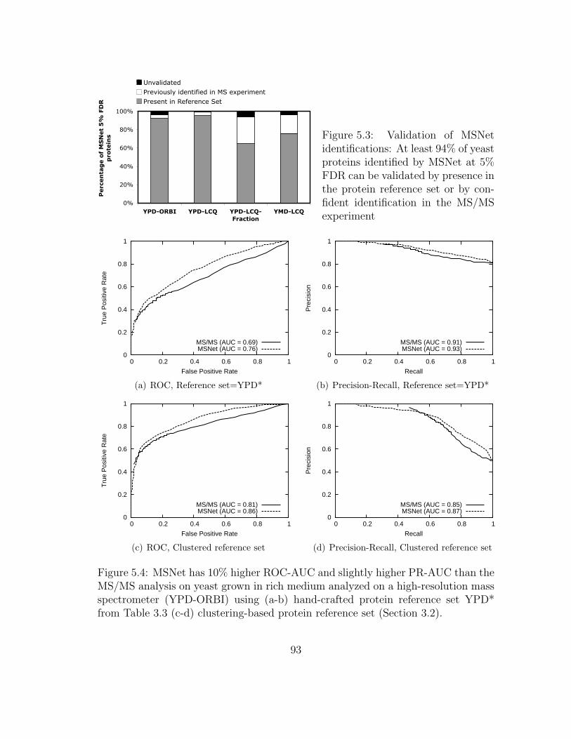
0%

20%

40%

60%

80%

100%

YPD-ORBI YPD-LCQ YPD-LCQ-

Fraction

YMD-LCQ

Percen

tag

e o

f M

SN

et

5%

FD

R

pro

tein

s

Unvalidated

Previously identified in MS experiment

Present in Reference Set

Figure 5.3: Validation of MSNetidentifications: At least 94% of yeastproteins identified by MSNet at 5%FDR can be validated by presence inthe protein reference set or by con-fident identification in the MS/MSexperiment

0

0.2

0.4

0.6

0.8

1

0 0.2 0.4 0.6 0.8 1

Tru

e P

ositi

ve R

ate

False Positive Rate

MS/MS (AUC = 0.69)MSNet (AUC = 0.76)

(a) ROC, Reference set=YPD*

0

0.2

0.4

0.6

0.8

1

0 0.2 0.4 0.6 0.8 1

Pre

cisi

on

Recall


(b) Precision-Recall, Reference set=YPD*

0

0.2

0.4

0.6

0.8

1

0 0.2 0.4 0.6 0.8 1

Tru

e P

ositi

ve R

ate

False Positive Rate


(c) ROC, Clustered reference set

0

0.2

0.4

0.6

0.8

1

0 0.2 0.4 0.6 0.8 1

Pre

cisi

on

Recall


(d) Precision-Recall, Clustered reference set

Figure 5.4: MSNet has 10% higher ROC-AUC and slightly higher PR-AUC than theMS/MS analysis on yeast grown in rich medium analyzed on a high-resolution massspectrometer (YPD-ORBI) using (a-b) hand-crafted protein reference set YPD*from Table 3.3 (c-d) clustering-based protein reference set (Section 3.2).

93

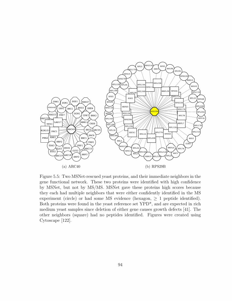
(a) ARC40 (b) RPS29B

Figure 5.5: Two MSNet-rescued yeast proteins, and their immediate neighbors in thegene functional network. These two proteins were identified with high confidenceby MSNet, but not by MS/MS. MSNet gave these proteins high scores becausethey each had multiple neighbors that were either confidently identified in the MSexperiment (circle) or had some MS evidence (hexagon, ≥ 1 peptide identified).Both proteins were found in the yeast reference set YPD*, and are expected in richmedium yeast samples since deletion of either gene causes growth defects [41]. Theother neighbors (square) had no peptides identified. Figures were created usingCytoscape [122].

94

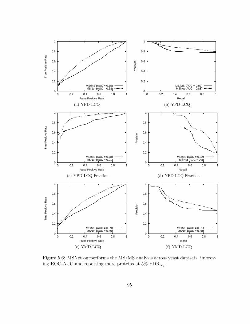
0

0.2

0.4

0.6

0.8

1

0 0.2 0.4 0.6 0.8 1

Tru

e P

ositi

ve R

ate

False Positive Rate


(a) YPD-LCQ

0

0.2

0.4

0.6

0.8

1

0 0.2 0.4 0.6 0.8 1

Pre

cisi

on

Recall


(b) YPD-LCQ

0

0.2

0.4

0.6

0.8

1

0 0.2 0.4 0.6 0.8 1

Tru

e P

ositi

ve R

ate

False Positive Rate


(c) YPD-LCQ-Fraction

0

0.2

0.4

0.6

0.8

1

0 0.2 0.4 0.6 0.8 1

Pre

cisi

on

Recall


(d) YPD-LCQ-Fraction

0

0.2

0.4

0.6

0.8

1

0 0.2 0.4 0.6 0.8 1

Tru

e P

ositi

ve R

ate

False Positive Rate


(e) YMD-LCQ

0

0.2

0.4

0.6

0.8

1

0 0.2 0.4 0.6 0.8 1

Pre

cisi

on

Recall


(f) YMD-LCQ

Figure 5.6: MSNet outperforms the MS/MS analysis across yeast datasets, improv-ing ROC-AUC and reporting more proteins at 5% FDRref .

95

0%

20%

40%

60%

80%

100%

Bioworks-

TPP

X!Tandem-

TPP

2-CRUX-

Percolator

1-CRUX-

Percolator

Average

Percen

t o

f M

SN

et

5%

FD

R p

ro

tein

s

Unvalidated

Previously identified in MS experiment

Present in Reference Set

Figure 5.7: Results using different MS/MS software pipelines: MSNet was run onprotein identification data from different MS/MS analysis pipelines on the samesample (YPD-ORBI). For all but the adhoc ‘Average’ pipeline (we computed averageprotein probability by averaging scores from the first three pipelines), at least 93%of MSNet 5% FDR identifications were validated by presence in the reference set orby confident MS/MS identification

96

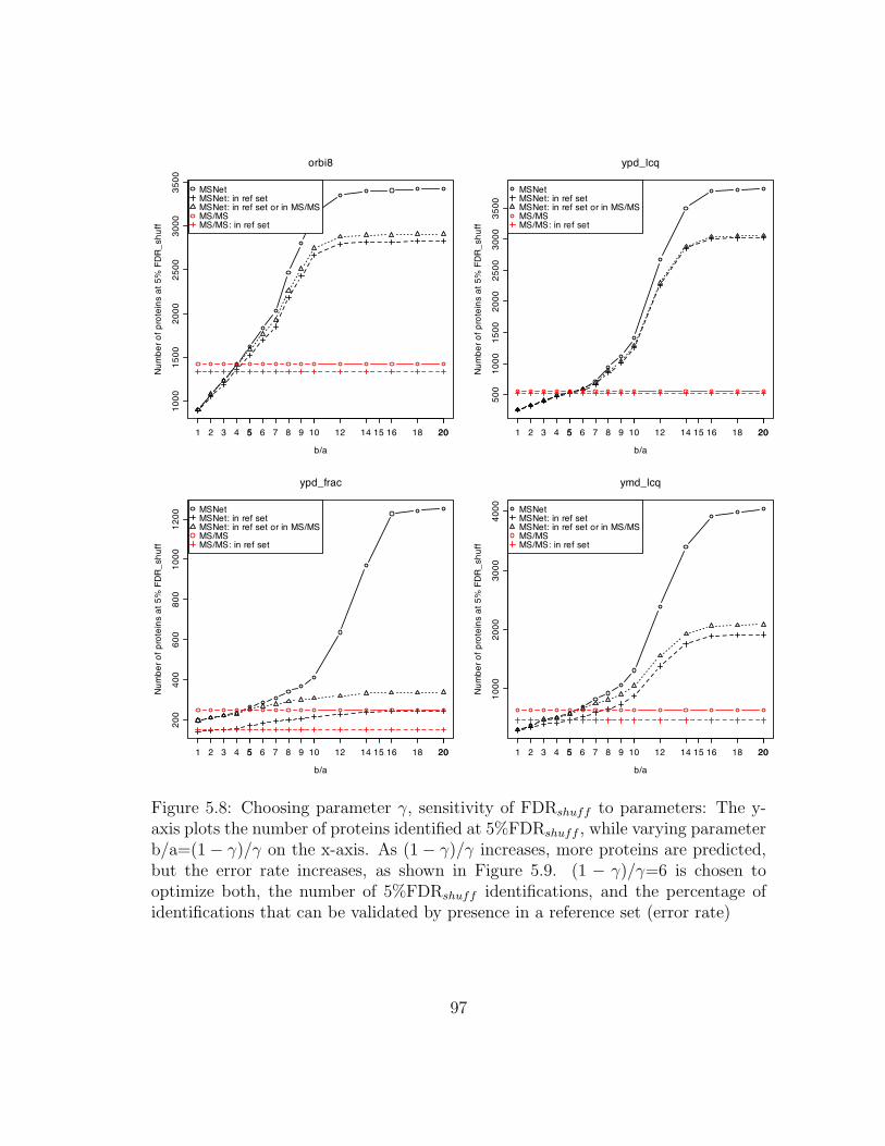
5 10 15 20

10

00

15

00

20

00

25

00

30

00

35

00

1 2 3 4 5 6 7 8 9 12 14 16 18 20

orbi8

b/a

Nu

mb

er

of

pro

tein

s a

t 5

% F

DR

_sh

uff

MSNetMSNet: in ref setMSNet: in ref set or in MS/MSMS/MSMS/MS: in ref set

5 10 15 20

50

01

00

01

50

02

00

02

50

03

00

03

50

0

1 2 3 4 5 6 7 8 9 12 14 16 18 20

ypd_lcq

b/a

Nu

mb

er

of

pro

tein

s a

t 5

% F

DR

_sh

uff


5 10 15 20

20

04

00

60

08

00

10

00

12

00

1 2 3 4 5 6 7 8 9 12 14 16 18 20

ypd_frac

b/a

Nu

mb

er

of

pro

tein

s a

t 5

% F

DR

_sh

uff


5 10 15 20

10

00

20

00

30

00

40

00

1 2 3 4 5 6 7 8 9 12 14 16 18 20

ymd_lcq

b/a

Nu

mb

er

of

pro

tein

s a

t 5

% F

DR

_sh

uff


Figure 5.8: Choosing parameter γ, sensitivity of FDRshuff to parameters: The y-axis plots the number of proteins identified at 5%FDRshuff , while varying parameterb/a=(1 − γ)/γ on the x-axis. As (1 − γ)/γ increases, more proteins are predicted,but the error rate increases, as shown in Figure 5.9. (1 − γ)/γ=6 is chosen tooptimize both, the number of 5%FDRshuff identifications, and the percentage ofidentifications that can be validated by presence in a reference set (error rate)

97

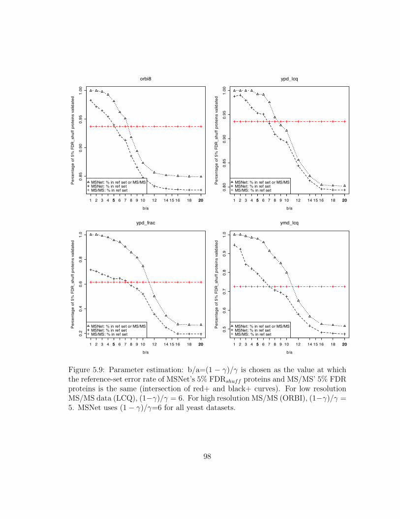
5 10 15 20

0.8

50

.90

0.9

51

.00

1 2 3 4 5 6 7 8 9 12 14 16 18 20

orbi8

b/a

Pe

rce

nta

ge

of

5%

FD

R_

sh

uff

pro

tein

s v

alid

ate

d

MSNet: % in ref set or MS/MSMSNet: % in ref setMS/MS: % in ref set

5 10 15 20

0.8

00

.85

0.9

00

.95

1.0

0

1 2 3 4 5 6 7 8 9 12 14 16 18 20

ypd_lcq

b/a

Pe

rce

nta

ge

of

5%

FD

R_

sh

uff

pro

tein

s v

alid

ate

d


5 10 15 20

0.2

0.4

0.6

0.8

1.0

1 2 3 4 5 6 7 8 9 12 14 16 18 20

ypd_frac

b/a

Pe

rce

nta

ge

of

5%

FD

R_

sh

uff

pro

tein

s v

alid

ate

d


5 10 15 20

0.5

0.6

0.7

0.8

0.9

1.0

1 2 3 4 5 6 7 8 9 12 14 16 18 20

ymd_lcq

b/a

Pe

rce

nta

ge

of

5%

FD

R_

sh

uff

pro

tein

s v

alid

ate

d


Figure 5.9: Parameter estimation: b/a=(1 − γ)/γ is chosen as the value at whichthe reference-set error rate of MSNet’s 5% FDRshuff proteins and MS/MS’ 5% FDRproteins is the same (intersection of red+ and black+ curves). For low resolutionMS/MS data (LCQ), (1−γ)/γ = 6. For high resolution MS/MS (ORBI), (1−γ)/γ =5. MSNet uses (1− γ)/γ=6 for all yeast datasets.

98

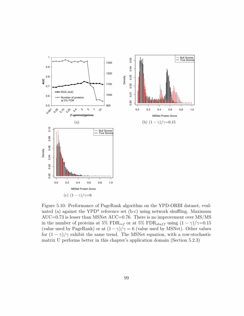
ypd_orbi8_cvogel Chart 5

Page 1

0.5

0.6

0.7

0.8

0.9

1

0.00

10.

050.

150.

25 0.4 2 5 7 10

(1-gamma)/gamma

AUC

900

1000

1100

1200

1300

ROC-AUC

Number of proteinsat 5% FDR

(a)

0.0 0.2 0.4 0.6 0.8 1.0

0.00

0.01

0.02

0.03

0.04

0.05

Null ScoresTrue Scores

MSNet Protein Score

Dens

ity(b) (1− γ)/γ=0.15

0.0 0.2 0.4 0.6 0.8 1.0

0.00

0.02

0.04

0.06

0.08

0.10 Null Scores

True Scores

MSNet Protein Score

Dens

ity

(c) (1− γ)/γ=6

Figure 5.10: Performance of PageRank algorithm on the YPD-ORBI dataset, eval-uated (a) against the YPD* reference set (b-c) using network shuffling. MaximumAUC=0.73 is lesser than MSNet AUC=0.76. There is no improvement over MS/MSin the number of proteins at 5% FDRref or at 5% FDRshuff using (1 − γ)/γ=0.15(value used by PageRank) or at (1−γ)/γ = 6 (value used by MSNet). Other valuesfor (1 − γ)/γ exhibit the same trend. The MSNet equation, with a row-stochasticmatrix U performs better in this chapter’s application domain (Section 5.2.3)

99

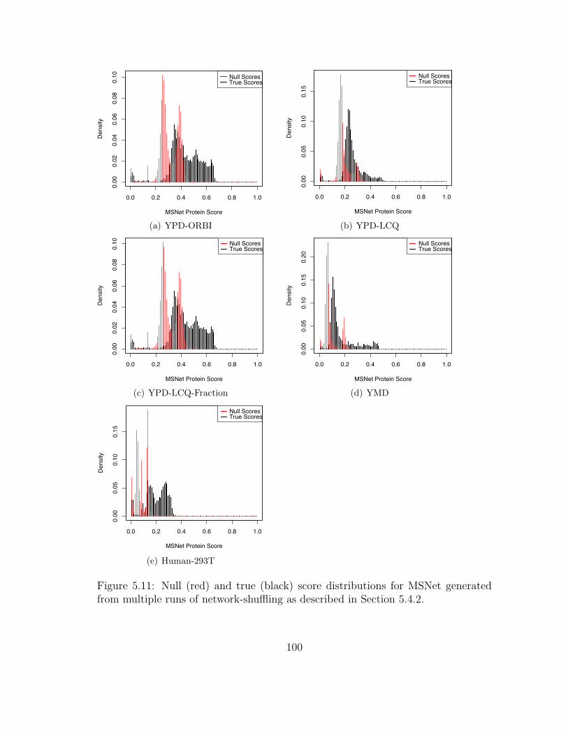
0.0 0.2 0.4 0.6 0.8 1.0

0.00

0.02

0.04

0.06

0.08

0.10 Null Scores

True Scores

MSNet Protein Score

Dens

ity

(a) YPD-ORBI

0.0 0.2 0.4 0.6 0.8 1.0

0.00

0.05

0.10

0.15


MSNet Protein Score

Dens

ity

(b) YPD-LCQ

0.0 0.2 0.4 0.6 0.8 1.0

0.00

0.02

0.04

0.06

0.08

0.10 Null Scores

True Scores

MSNet Protein Score

Dens

ity

(c) YPD-LCQ-Fraction

0.0 0.2 0.4 0.6 0.8 1.0

0.00

0.05

0.10

0.15

0.20


MSNet Protein Score

Dens

ity

(d) YMD

0.0 0.2 0.4 0.6 0.8 1.0

0.00

0.05

0.10

0.15


MSNet Protein Score

Dens

ity

(e) Human-293T

Figure 5.11: Null (red) and true (black) score distributions for MSNet generatedfrom multiple runs of network-shuffling as described in Section 5.4.2.

100

Chapter 6

Network priors: graphical models and Markov

Random Fields

Probabilistic graphical models merge graph theory and probability theory

and are used to statistically model complex inter-dependencies between data ele-

ments. As defined by Kevin Murphy in his 1998 tutorial1, nodes in a graphical

model represent random variables, and the (lack of) arcs between nodes represent

conditional independence assumptions. The conditional independence assumptions

simplify the dependency structure, and make prediction tasks computationally more

feasible. Directed edges represent causality, in the sense that an event A is said to

have caused B with some probability if there is an edge from A to B. Directed

graphical models are called Bayesian networks [99]. Undirected graphical models

are called Markov networks or Markov Random Fields and represent more gen-

eral dependencies. They have traditionally been popular in statistical physics and

vision applications, with several recent applications biology e.g. network-aided pro-

tein/gene function prediction (as discussed in Section 5.7).

There are two steps to using a graphical model for prediction: learning the

model from data, and performing inference on the learned model. In this disserta-

tion, we focus on the application of graphical models to the protein identification

task. We represent protein experiment data (features of a node) and gene rela-

1current and maintained at http://www.cs.ubc.ca/ murphyk/Bayes/bnintro.html

101

tionships (edges between nodes) by an undirected graphical model, and treat the

protein identification task as a recommendation or prediction task over the graphical

model. To see this, define a Bernoulli random variable Xi = {0, 1} associated with

each node i in the gene graph. A subset of the N proteins in an organism’s proteome

is expected to be present in any given sample. The task is to infer the probability

of protein i being present given both experimental data and network dependencies

i.e. P (Xi = 1|protein experiment, network links).

6.1 Markov Random Fields

A graphical model has an associated joint probability distribution defined

over all variables (nodes) in the graph. Learning the parameters of the distribution

and inference on a parameterized model are both intractable for the general case of

graphs with arbitrary topology and arbitrary probability distributions. A theorem

by Hammersly and Clifford states that the necessary and sufficient conditions for a

probability distribution to be a MRF is that it is completely factorisable over fully-

connected subsets of nodes (cliques) [72]. This result is also known as the Markov-

Gibbs equivalence. The potential functions are restricted to being positive, but need

not themselves be probability distributions. As a result, a Markov network and its

joint probability distribution are completely characterized by potential functions

that take sets of fully-connected nodes (cliques) as arguments.

A pairwise MRF is a commonly adopted parametrization that considers the

set of edges (i, j) ∈ E as the set of cliques. A graphical model can be represented

as a pairwise MRF without loss of generality [147], and in what follows we only

discuss pairwise MRFs since they are easier to represent and conceptualize. A

Pairwise MRF is characterized by unary potential function(s) Fi(Xi) > 0, and a

102

binary potential function(s) Fij(Xi, Xj) > 0. Fij is generally defined to encourage

configurations where connected nodes are in similar states (Xi = Xj). With a slight

abuse in notation, the subscripts i and ij serve to distinguish between unary and

binary potential functions, as well as serve as subscripts to denote different variables

Xi and Xj. Using the Markov-Gibbs equivalence, we can write the joint distribution

of Xi in terms of Fi and Fij [72]:

P (X1, . . . , XN |data) ∝ P (data|X1×N)P (X1×N)

∝N∏i

Fi(Xi)∏

(i,j)∈E

Fij(Xi, Xj) (6.1)

The local Markov property of a Markov net states that the state of a node

depends only on the state of its immediate neighbors in the graph (Markov blanket,

[99]). As a result, the conditional probability of a node can be written only in terms

of potential functions that take the node as an argument. For a pairwise MRF, this

includes Fi(Xi) and Fij(Xi, Xj) for every edge (i, j) ∈ E:

P (Xi = 1|X¬i, {experiment,network})

∝ Fi(Xi = x)∏

(i,j)∈E

Fij(Xi = x,Xj)

∏k 6=i

Fi(Xk)∏

(k,l)∈E,k 6=i

Fij(Xk, Xl)

∝ Fi(Xi = x)

∏j:(i,j)∈E

Fij(Xi = x,Xj) (6.2)

6.2 Message-passing inference for graphical models

For a given instance of potential functions Fi, Fij on a graphical model, the

inference task is to find assignments to all unobserved variables Xu conditioned on

the observed values Xo. In the protein identification task, an assignment Xi = 1

implies that protein i is present in the sample. Inference has three associated sub-

103

tasks, as summarized by Yair Weiss in a series of seminal papers on the analysis of

the belief propagation [99] paradigm for inference in Bayesian networks [141]:

1. Marginalization: estimate the marginal probabilities of unobserved nodes given

observed data O, P (Xui |O).

2. Maximum a posteriori (MAP) assignment : find an assignment u1, u2, . . . , uk

to Xu such that the joint posterior probability P (Xu1 = u1, . . . , X

uk = uk|O) is

maximized.

3. Maximum marginal (MM) assignment : find an assignment u1, u2, . . . , uk to

Xu such that all the marginal probabilities P (Xu1 = u1|O), . . . , P (Xu

k = uk|O)

are maximized.

Our aim is to estimate the probability of protein presence as the marginal prob-

abilities P (Xui |Xo, data) conditioned on observed nodes Xo that result in a MAP

configuration, and then estimate significance thresholds on this ranked list of prob-

abilities as usual.

Complexity of inference in graphical models : Exact inference involves marginal-

ization over unobserved nodes. This marginalization is exponential in the number

of nodes, or in the ‘tree-width’ of an acyclic graph, and computationally infeasible

for anything but small graphs, necessitating approximate methods. Further, since

even approximate inference within a constant factor approximation is NP-hard [21],

recent approaches estimate error bounds on the approximate marginal probabili-

ties [112].

Pearl introduced belief propagation (BP) as an inference algorithm for di-

rected graphical models (Bayesian networks) [99]. BP is a message-passing algo-

104

rithm that performs exact inference on acyclic graphs in time linear in the number

of nodes. Each iteration of the BP algorithm computes a belief for each node i.

For acyclic graphs, BP converges in two iterations, and the computed belief B(Xui )

at an unobserved node is equal to the marginal probability P (Xui |Xo) conditioned

on the observed nodes Xo (Equation 6.2) [98]. The belief is a p-dimensional vector

where Xui is a p-valued discrete RV. Belief propagation can be applied to graphs

with cycles, and in this form is called loopy belief propagation (LBP). Convergence

is not guaranteed with cycles, but when the algorithm does converge it has shown

extremely good empirical performance [141].

BP falls into a class of general message-passing algorithms. Kschischang, Frey

and Loeliger [67] placed belief propagation into an elegant framework called factor

graphs. The factor graph framework speaks to algorithms that deal with a complex

global function of many variables by factorizing it into functions that operate on

smaller sets of variables (factors). In the case of probabilistic models, the global

function is a probability distribution over the entire graph. The factor functions are

conditional probability distributions in Bayesian networks and potential functions in

Markov networks. A factor graph is a bipartite graph between variables and factors

functions. The edges connect functions to their argument variables. Sum-product

and max-product algorithms are message-passing algorithm for inference in factor

graphs, with equivalence to the belief propagation and belief revision algorithms

introduced by Pearl. Messages are passed between functions and their arguments.

We adopt the factor graph notation and terminology in the sections that follow,

clarifying connections to belief propagation terminology where applicable.

The sum-product and max-product message-passing algorithms have good

performance and convergence properties on our parametrization of factor graphs

105

for protein identification. In this dissertation, we do not empirically evaluate other

approximate inference frameworks e.g. variational methods beyond sum-product

inference [136], stochastic Markov Chain Monte Carlo (MCMC) methods [66], or

discriminative random field methods [68]. We compare against one other method

based on Gaussian fields, that has been successful in network-based prediction of

gene function. Inference in Gaussian fields can be achieved by solving a convex

optimization problem using the graph Laplacian. This method results in ROC-

AUC comparable to MSNet, but suffers from low precision at low FDR (region of

interest) (Section 6.4).

6.2.1 Sum-product algorithm (belief propagation)

First, some notation to standardize the description of the algorithm 2

1. Neighborhood ∆Xi is the set of all factor functions of which Xi is an argu-

ment.

2. Neighborhood ∆F is the set of all arguments of F .

3. µ(t)F→Xi

(x) is the xth element of the message vector from function F to node

Xi ∈ ∆F , at the tth iteration. If Xi is Bernoulli, the message is a vector of

length two, x = 0, 1.

4. ν(t)X→F (x) is the xth element of the message from node X ∈ ∆F to function F

at the tth iteration.

2The sum-product literature spans more than two decades, and notations differ based on theapplication domain of this ubiquitous algorithm. The notation in this section is adapted from arecent description of the sum-product algorithm in [92]. [99] and [67] are traditional references.

106

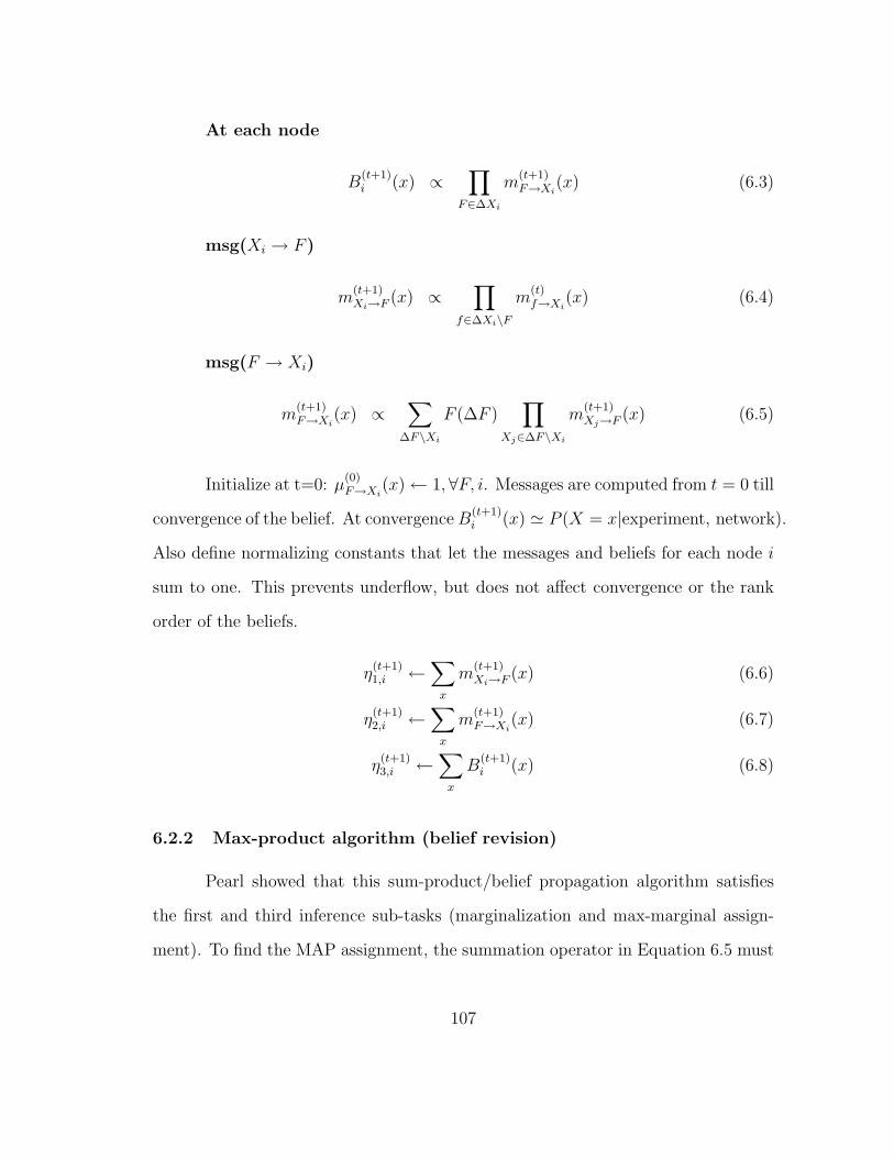
At each node

B(t+1)i (x) ∝

∏F∈∆Xi

m(t+1)F→Xi

(x) (6.3)

msg(Xi → F )

m(t+1)Xi→F (x) ∝

∏f∈∆Xi\F

m(t)f→Xi

(x) (6.4)

msg(F → Xi)

m(t+1)F→Xi

(x) ∝∑

∆F\Xi

F (∆F )∏

Xj∈∆F\Xi

m(t+1)Xj→F (x) (6.5)

Initialize at t=0: µ(0)F→Xi

(x)← 1,∀F, i. Messages are computed from t = 0 till

convergence of the belief. At convergenceB(t+1)i (x) ' P (X = x|experiment, network).

Also define normalizing constants that let the messages and beliefs for each node i

sum to one. This prevents underflow, but does not affect convergence or the rank

order of the beliefs.

η(t+1)1,i ←

∑x

m(t+1)Xi→F (x) (6.6)

η(t+1)2,i ←

∑x

m(t+1)F→Xi

(x) (6.7)

η(t+1)3,i ←

∑x

B(t+1)i (x) (6.8)

6.2.2 Max-product algorithm (belief revision)

Pearl showed that this sum-product/belief propagation algorithm satisfies

the first and third inference sub-tasks (marginalization and max-marginal assign-

ment). To find the MAP assignment, the summation operator in Equation 6.5 must

107

be replaced by a maximization operator. An assignment based on marginal prob-

abilities computed by this max-product algorithm satisfies all inference sub-tasks.

Pearl called this modified algorithm belief revision [99].

In [142], Weiss showed that at fixed-point, the max-product assignment is a

‘neighborhood maximum of the posterior probability - the max-product assignment

is guaranteed to be better than all other assignments in a large region around the

assignment’. He used this property to explain the excellent empirical performance

of max-product on arbitrary graphs with cycles in convergent cases. His conclu-

sions were that max-product outperforms sum-product in convergent cases, but is

known to converge less often. Results using both sum-product and max-product are

presented in Section 6.5. Max-product inference slightly outperformed sum-product

inference when the assignments were evaluated against a benchmarking set, and also

took more iterations to converge.

6.3 An MRF model on gene networks

6.3.1 Model definition

We defined unary and binary factor functions based on the availability of the

functional network and MS and mRNA data3. As detailed in Section 5.2, oi is a

sample-specific probability of protein presence based on an MS/MS experiment on

that sample (Equation 5.2). G(V,E) is an undirected weighted graph with |V | = N

vertices corresponding to the proteins, and weighted edges eij = (i, j, wij) ∈ E. qij

is the probability that proteins i and j are functionally related, derived by a logistic

transformation on wij, the log-likelihood-odds of a functional link. In an unweighted

3William H Press, personal communication, May 2009

108

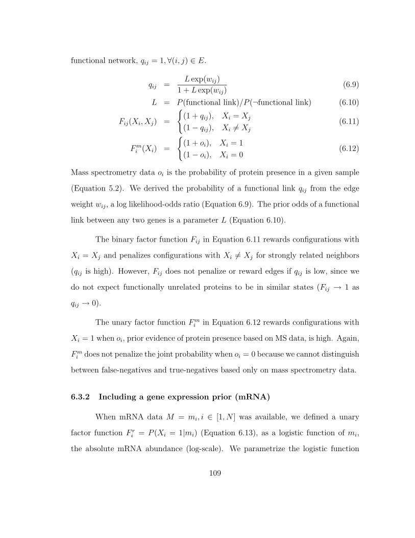
functional network, qij = 1,∀(i, j) ∈ E.

qij =L exp(wij)

1 + L exp(wij)(6.9)

L = P (functional link)/P (¬functional link) (6.10)

Fij(Xi, Xj) =

{(1 + qij), Xi = Xj

(1− qij), Xi 6= Xj

(6.11)

Fmi (Xi) =

{(1 + oi), Xi = 1

(1− oi), Xi = 0(6.12)

Mass spectrometry data oi is the probability of protein presence in a given sample

(Equation 5.2). We derived the probability of a functional link qij from the edge

weight wij, a log likelihood-odds ratio (Equation 6.9). The prior odds of a functional

link between any two genes is a parameter L (Equation 6.10).

The binary factor function Fij in Equation 6.11 rewards configurations with

Xi = Xj and penalizes configurations with Xi 6= Xj for strongly related neighbors

(qij is high). However, Fij does not penalize or reward edges if qij is low, since we

do not expect functionally unrelated proteins to be in similar states (Fij → 1 as

qij → 0).

The unary factor function Fmi in Equation 6.12 rewards configurations with

Xi = 1 when oi, prior evidence of protein presence based on MS data, is high. Again,

Fmi does not penalize the joint probability when oi = 0 because we cannot distinguish

between false-negatives and true-negatives based only on mass spectrometry data.

6.3.2 Including a gene expression prior (mRNA)

When mRNA data M = mi, i ∈ [1, N ] was available, we defined a unary

factor function F ri = P (Xi = 1|mi) (Equation 6.13), as a logistic function of mi,

the absolute mRNA abundance (log-scale). We parametrize the logistic function

109

−1 0 1 2 3

0.0

0.2

0.4

0.6

0.8

1.0

MSpressoLogistic (D=3)

mRNA concentration (log base 10)

Pro

babi

lity Figure 6.1: Plot of the logistic fac-

tor function F ri for the mRNA-

MRF model (Equation 6.13), whichis more conservative at lower mRNAabundances (∼ 1 mol/cell), andslightly anti-conservative at highermRNA abundances (> 10 mol/cell)than MSPresso’s P (K = 1|M), theprobability of protein presence givenmRNA abundance M (Chapter 4)

based our previously learned relationship between mRNA abundance and protein

presence (Section 4.2.1, Figure 4.2). Parameter D scales the logistic function and

we optimized it using cross-validation on ground-truth reference sets. We defined a

combined unary factor function Fi as the product of mRNA and MS/MS factors:

F ri (Xi) =

{eDmi

1+eDmi, Xi = 1

11+eDmi

, Xi = 0(6.13)

Fi(Xi) = Fmi (Xi)F

ri (Xi) (6.14)

6.4 Gaussian field label propagation

We can formulate a quadratic objective function f(Y )4 that seeks to minimize

(a) a local penalty: the deviation of the final probabilities from the original mass-

spectrometry probabilities and (b) a neighborhood-penalty: the deviation between

neighboring nodes Xi 6= Xj, (i, j) ∈ E. The neighborhood penalty is weighted by

4Inderjit Dhillon, personal communication, January 2009

110

wij. This cost function is also used by GeneMania, a tool for network-assisted gene

function prediction [87].

Y ∗ = argminY

f(Y ) (6.15)

f(Y ) =∑

(i,j)∈E

wij(yi − yj)2 +∑i

(yi − oi)2 (6.16)

The cost function can be written in matrix form by defining Z, an indicator vector

with zi = 1 if oi > 0 (protein observed in the MS/MS experiment), WN×N is the

weighted adjacency matrix of G, the graph Laplacian LG = D −W where DN×N

is a diagonal weighted degree matrix (Dii =∑

j wij). Since LG is generated from

the adjacency matrix of the gene network graph in [70] is positive-semidefinite by

construction of the network, the minimization is a convex optimization problem.

Results of ranking proteins based on Y ∗, the minimizer of f(Y ), are in Section 6.55.

f(Y ) = Y TLGY + (Y −O)TZ(Y −O) (6.17)

df

dy= 0 ⇒ LGY + Z(Y −O) = 0

⇒ Y ∗ = (LG + Z)−1ZO (6.18)

6.5 Results

6.5.1 Evaluation Methodology

The evaluation set consisted of proteins with data from all three sources: at

least one peptide identified in the MS/MS experiment, non-zero absolute mRNA

abundance and at least one edge in the gene functional network. We restricted

evaluation to this common subset of proteins to enable comparison of ROC and

precision-recall curves across models. Note that we used all proteins with available

5Results generated by Peggy Wang’s Matlab implementation

111

data for training the individual models, and only restricted the size of the evaluation

set.

We measured performance by the areas under ROC and precision-recall

curves (AUC-ROC, AUC-PR), using the reference sets described in Table 3.3 as

ground-truth. Posterior probabilities were averaged over two runs of ten-fold cross

validation.

6.5.2 Evaluation

We ran the iterative sum-product and max-product algorithms on yeast

grown in rich medium analyzed on an LTQ-Orbitrap mass spectrometer (Table

3.1, YPD-ORBI) using the yeast functional network used in Chapter 5. The MRF

model is dubbed ‘MRF’, and the model with mRNA data is ‘mRNA-MRF’.

We measured algorithm convergence if the L2 norm error between belief

vectors at t and (t − 1)th iterations was < ε for N consecutive iterations. For a

dataset of ∼5000 proteins, ε = 10−5 and N = 5, the algorithm converged in few tens

of iterations. All messages and beliefs were normalized to sum to one.

The areas under ROC and precision-recall curves (AUC-ROC, AUC-PR)

were sensitive to choice of parameter L=prior-odds(function link) (Equation 6.10).

In particular, performance rapidly degraded for L>0.005, which corresponds to

P(link)=5 × 10−3. We chose parameters {D,L} to maximize average AUC-ROC,

AUC-PR and number of proteins at 5% FDR (Figure 6.2, best L = 0.005, D = 3).

ROC and Precision-Recall plots for MRF and mRNA-MRF are shown in Figure 6.3.

112

cvr2f10_summary_balance_balance Chart 5

Page 1

0.5

0.6

0.7

0.8

5.00E-

04

0.001 0.005 0.01 0.05 0.9 2 9L

AU

C

1000

1100

1200

1300

1400

1500

1600

Nu

mb

er p

rote

ins a

t 5%

FD

R

AUC-ROC (MRF)AUC-ROC (MS)Num prots (MRF)Num prots (MS)

(a) Varying L

cvr2f10_summary_mlogitDvary_qba Chart 3

Page 1

0.6

0.65

0.7

0.75

0.8

0.5 1.5 2.5 3.5 4.5 5.5 6.5 7.5

D (L = 0.005)A

UC

1300

1400

1500

1600

1700

1800

Nu

m p

rote

ins a

t 5%

FD

R

AUC-ROC (MRF)AUC-ROC (MS)Num prots (MRF)Num prots (MS)

(b) Varying D for optimal L=0.005

0.51.52.5

0.5

0.6

0.7

0.80.76 0.76 0.77

0.76

0.64

0.540.53

0.52

D

ROC‐AUC

L

(c) Varying D and L, AUC

0.5

1.5

2.5

100011001200130014001500160017001800

1600 1616 17191681

D

Num

. proteins at 5% FDR

L

(d) Varying D and L, proteins at 5% FDR

Figure 6.2: Choosing MRF parameters (D,L) by optimizing cross-validated ROC-AUC and number of proteins at 5% FDR, using the YPD* reference set as groundtruth. We choose L = 0.005, D = 3.

113

0

0.2

0.4

0.6

0.8

1

0 0.2 0.4 0.6 0.8 1

Tru

e P

ositi

ve R

ate

False Positive Rate


(a) ROC (MRF)

0

0.2

0.4

0.6

0.8

1

0 0.2 0.4 0.6 0.8 1

Pre

cisi

on

Recall


(b) Precision-Recall (MRF)

0

0.2

0.4

0.6

0.8

1

0 0.2 0.4 0.6 0.8 1

Tru

e P

ositi

ve R

ate

False Positive Rate


(c) ROC (mRNA-MRF)

0

0.2

0.4

0.6

0.8

1

0 0.2 0.4 0.6 0.8 1

Pre

cisi

on

Recall


(d) Precision-Recall (mRNA-MRF)

Figure 6.3: (a-b) The MRF model has 6% higher ROC-AUC than the MS/MSexperiment (L=0.005) (c-d) The mRNA-MRF model has 12% higher ROC-AUCthan the MS/MS experiment (D = 3,L=0.005). Both models maintain or increasearea under the Precision-Recall curve (PR-AUC).

114

Table 6.1: Comparison of all the integrative analysis models on the yeast YPD-ORBI dataset using the YPD* reference set as ground truth. As expected, themodel that uses both mRNA and network-based evidence performs the best at5%FDR (mRNA-MRF, D=3, L=0.005), followed by network-based models MRF(L=0.005) and MSNet (1−γ

γ=6). The Gaussian field performs poorly at low FDR

regions (*- not cross-validated)Model ROC 5% FDRref

AUC % Increase overMS experiment

Num.proteins

% Increase overMS experiment

MS experiment 0.69 - 1476 -MSPresso 0.75 9 1490 1MSNet 0.75 9 1566 6MRF 0.73 6 1589 8Gaussian field∗ 0.74 9 1243 <0mRNA-MRF 0.77 12 1719 16

6.5.3 Comparison to MSNet and MSPresso

We compared the performance of the two MRF models with our previous

MSPresso and MSNet models on the same dataset (Table 6.1). The best performing

MRF model (L=0.005) performed equivalently to the MSNet model of Chapter 5,

both outperforming the mRNA-only MSPresso model. As expected, the mRNA-

MRF model that uses all three data sources resulted in the highest number of

5% FDR identifications (6% higher). All four models had similar AUC-ROC, but

the models that use more data perform better at the 5% FDR cutoff, which is

the interesting region for high-throughput studies since it contains the confident

identifications.

6.5.4 Discussion

The principled probabilistic MRF framework supports adding new data sources

that are indicative of protein presence. Further, the score of a protein has a prob-

115

abilistic interpretation: it is the posterior marginal probability of a node of the

defined MRF. However, the general sum-product algorithm does not have the con-

vergence guarantee of the MSNet model. In the next section, we discuss a mapping

of the MSNet model into a Markov Random Field framework.

6.6 MSNet in a Markov Random Field framework

6.6.1 Model definition

In this section, we discuss the implications of placing the MSNet model of

Chapter 5 into a Markov Random Field framework with binary variables Xi. Specifi-

cally, we show that the MSNet score yi (Equation 5.4) is proportional to the log-odds

of the conditional probability of Xi if the binary factor function of the associated

MRF is defined in terms of the posterior marginals.

The unary factor function Fi of this MRF is defined in terms of the mass-

spectrometry protein probability (oi). The binary factor function Fij is defined in

terms of the edge weights wij and Bj, the posterior marginal probabilities of i’s

network neighbors:

Fi(Xi) =

{eγoi , Xi = 1

eγ(1−oi), Xi = 0(6.19)

Fij(Xi, Xj) = exp

(δwij

(Gij(Xi, Xj)∑

j wij+Gij(Xj, Xi)∑

iwij

))(6.20)

Gij(Xi, Xj) =

{Bj Xi = 1

(1−Bj) Xi = 0(6.21)

γ, δ > 0

where Bj is the posterior marginal probability P (Xj = 1|network, mass-spec data).

Recall that the beliefs computed by belief revision converge to the posterior marginals

(or approximations thereof for graphs with cycles). When running belief revision

116

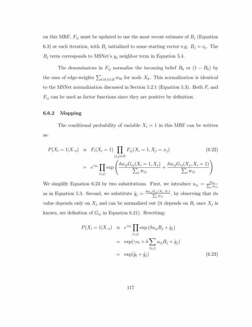
on this MRF, Fij must be updated to use the most recent estimate of Bj (Equation

6.3) at each iteration, with Bj initialized to some starting vector e.g. Bj = oj. The

Bj term corresponds to MSNet’s yj neighbor term in Equation 5.4.

The denominators in Fij normalize the incoming belief Bk or (1 − Bk) by

the sum of edge-weights∑

l:(k,l)∈E wkl for node Xk. This normalization is identical

to the MSNet normalization discussed in Section 5.2.1 (Equation 5.3). Both Fi and

Fij can be used as factor functions since they are positive by definition.

6.6.2 Mapping

The conditional probability of variable Xi = 1 in this MRF can be written

as:

P (Xi = 1|X¬i) ∝ Fi(Xi = 1)∏

(i,j)∈E

Fij(Xi = 1, Xj = xj) (6.22)

= eγoi

∏(i,j)

exp

(δwijGij(Xi = 1, Xj)∑

j wij+δwijGij(Xj, Xi = 1)∑

iwij

)

We simplify Equation 6.23 by two substitutions. First, we introduce uij =wijPj wij

as in Equation 5.3. Second, we substitute gj =δwijGij(Xj ,Xi)P

i wij, by observing that its

value depends only on Xj and can be normalized out (it depends on Bi once Xj is

known, see definition of Gij in Equation 6.21). Rewriting:

P (Xi = 1|X¬i) ∝ eγoi

∏(i,j)

exp (δuijBj + gj)

= exp(γoi + δ∑(i,j)

uijBj + gj)

= exp(yi + gj) (6.23)

117

where yi = γoi + δ∑

(i,j) uijBj. Note that yi has the same form as the MSNet score

yi in Equation 5.4. P (Xi = 0|X¬i) can be defined similarly in terms of yi and gi:

P (Xi = 0|X¬i) ∝ Fi(Xi = 0)∏(i,j)

Fij(Xi = 0, Xj = xj)

= eγ(1−oi)∏(i,j)

exp(δuij(1−Bj) + gj)

= exp((γ + δ∑(i,j)

uij)− (γoi + δ∑(i,j)

uijBj) + gj)

= exp (γ + δ − yi + gj) (6.24)

since∑

(i,j) uij = 1. Finally, we can define the log-odds of P (Xi|X¬i) as:

log

(P (Xi = 1|X¬i)P (Xi = 0|X¬i)

)= log

(exp (yi + gj)

exp (γ + δ − yi + gj)

)= 2yi − (γ + δ)

= 2γoi + 2δ∑(i,j)

uijBj − (γ + δ) (6.25)

Since γ, δ > 0 and γ + δ is constant ∀i, scores computed by Equation 6.25 are

rank-order equivalent to MSNet scores from Equation 5.4. In other words, the

MSNet score for protein i is proportional to log-odds of the conditional probability

of variable Xi in a MRF that is parameterized by Equations 6.19-6.22.

118

Chapter 7

MSFound: database indexing for peptide spectra

identification

7.1 Introduction

Two factors have contributed to the growing accessibility of large-scale MS/MS

proteomics: high throughput data acquisition capabilities of modern instrumenta-

tion and public availability of gene and protein sequence databases. Both factors

also necessitate computational methods to analyze spectral data, as described in

Section 2.1. Most of the analysis time is spent in the database search phase that

matches experimental and theoretical spectra. Post-processing to compute pep-

tide and protein scores takes only a few minutes in comparison. It can take about

forty minutes to analyze one typical run from an LC/LC/MS/MS high-resolution

spectrometer using BioWorks (human sample). In practice, biologists run multiple

technical replicates of the same experiment. For instance, our human dataset (Ta-

ble 7.1, Human-DAOY-ORBI) consisted of ten technical replicates, and the overall

computational analysis took between five and six hours.

Run time is largely determined by the size of the database and by the compu-

tational complexity of the distance metrics used to compare spectra. For instance,

searches are exponentially slower when searching for unrestricted1 post-translational

modifications. Searches are also slower by a linear factor when a target-decoy strat-

1Searching for all possible PTMs across several sites on a protein

119

egy is used for error estimation since the decoy proteins double the size of the

database (Section 2.4.1).

Since relational database systems often form the storage layer for mass spec-

trometry spectra collections [85,134], we developed a database indexing solution to

improve search speed and scalability of mass spectra database search. A linear scan

of a database without an index involves comparing every object in the database

against the query object to select a set of search results. A database index is a

data structure that organizes the data to reduce this number of comparisons, hence

resulting in faster searches.

Objects are usually compared using some notion of distance e.g. Euclidean

distance for vectors, or Smith-Waterman alignment score for sequences. Distance-

based indexing has been used effectively in spatial and image databases using KD-

trees [6] or R trees [46] for 2-3 dimensional objects. Metric space indexing is a

generalization of these methods, in which distances need not correspond to any

coordinate axis system, as long as they satisfy the properties of a metric distance.

This is the approach adopted by the Molecular Biological Database (MoBIoS) [22]

system comprising a disk-based metric-space indexing data structure and nearest

neighbor search algorithms. Typical database entities in MoBIoS are gene and

protein sequences and mass spectra with corresponding distance metrics. MoBIoS

aims to store general-purpose data structures that support fast scalable retrieval of

complex data types. Metric-space indexing techniques achieve speedup by employing

the triangle-inequality property of a metric distance to prune data points from the

result set. In other words, the number of distance computations between data points

is reduced, which reduces overall search time.

Our system, MS-Found [109], was the first to formulate a fast, scalable

120

database indexing solution to this problem, and has since been followed by other in-

dexing methods [29,37]. MS-Found has been incorporated in the MoBIoS biological

database management system and is available as a web-service.

7.2 Methods

7.2.1 Metric space indexing for database search

A metric space (M, Dmet) is defined by a non-empty set of data points M and

a non-negative real distance function Dmet(m1,m2) : M ×M → < between pairs of

points in M, that satisfies the following conditions:

1. Dmet(m1,m2) = 0 iff m1 = m2 (identity)

2. Dmet(m1,m2) = Dmet(m2,m1) (symmetry)

3. Dmet(m1,m2) +Dmet(m2,m3) ≥ Dmet(m1,m3) (triangle inequality)

Two common query types are: range queries, which return all data objects

within a certain distance R to the query, and k-nearest neighbor queries, which

return the k data objects with the smallest distance to the query. A third query

type is the radius bounded k-NN query which returns up to k points that are within

distance R from the query. A search predicate contains the query point and radius

R, or k or both based on the query type.

MoBIoS implements a metric-space, ball-tree based index structure. This

category of indexing structures recursively partitions the search space into overlap-

ping bounding spheres, creating an index tree. At query-time, the triangle inequality

is used to aggressively prune sub-sections of the tree that are unlikely to contain

results. MoBIoS implements a disk-based version of the Multiple Vantage Point

121

tree [10], which are derived from Vantage Point Trees (VP), which were proposed

independently by [132] and [149]. In a VP tree, the bounding sphere, defined by a

vantage point (or pivot) v and radius r, partitions the data into two evenly sized

subsets. A top-down recursive construction chooses a vantage point v and radius

r at each branch of each level, resulting in a balanced binary tree. Bozkaya et al.

extended this concept by introducing multiple vantage points per node (v), and/or

nesting multiple bounding spheres per vantage point (s) to form a Multiple Vantage

Point tree. When choosing the MVP tree structure for MoBIoS, Mao et al showed

that MVP-trees outperformed other metric-space indexing structures on a series of

real and simulated workloads (image, DNA, mass spectra, uniform d-dimensional

vector) [81].

Good choices of vantage points and bounding sphere radii are essential to the

effectiveness of the metric-space structure. The choice depends on the dimension-

ality, distribution and sparsity of the dataset. Details about constructing the MVP

trees in MoBIoS, including heuristics for choosing good vantage points are in [82].

A range query in a metric space may be implemented by traversing the in-

dex tree, starting from the root node. When an internal node is visited, the search

predicate is compared to the index predicate that is parameterized by pivots and

data points stored in that node. A sub-tree can be eliminated from further con-

sideration (pruning) if the query predicate has no overlap with the index predicate

that describes the points stored in that sub-tree. The triangle-inequality property

of metric-spaces is used to achieve this pruning guarantee. Specifically, in a metric

space search of radius r for query q, given an index pivot point p and a metric dis-

tance function d, we would prune all points u that satisfy Equation 7.1. Good radius

values r are application specific, and algorithm evaluation is usually performed over

122

a range of potential radii.

|d(u, pi)− d(q, pi)| > r (7.1)

Recent work in searching large, high-dimensional databases has focused on

approximate searches, since exact NN searches have space and/or time complexity

that grows exponentially with dimension. This implies that at high dimensions,

exact NN can degrade to a linear search, where each data point is compared to the

query point before being selected as a result or eliminated (O(n)).

Several methods have been proposed to solve approximate nearest-neighbor

(A-KNN) problems (See Section 7.2.2) that vary based on the techniques used for

space partitioning, data representation and similarity measures. A recent survey

classifies various similarity search techniques into a taxonomy based on several as-

pects of the algorithm, e.g. supported data space and similarity functions, type of

approximation and type of guarantee on approximation error among others [83].

7.2.2 MoBIoS’ k-NN search algorithm

In adversarial, high dimensional spaces, naive k-NN algorithms can be more

expensive than a linear scan, due to the curse of dimensionality [120]. Thus, though

k-NN queries can be implemented using multiple range queries with increasing ra-

dius, other k-NN specific algorithms are used. A large portion of search time in

k-NN algorithms is spent in confirming that the top k results are indeed the k

nearest points. Approximate k-NN algorithms (A-KNN) sacrifice some accuracy for

speed in high-dimensional spaces: they return any point that is within (1 + ε) of

the true-nearest neighbor [42,150]. Another approach to A-KNN is to impose early

termination criteria based on running time, or the size of the searched neighbor-

hood [148]. Accuracy of returned results can be measured by relative error, which is

123

the average error of the result set to the true set of k closest points. A-KNN often

works very well for applications where a coarse-grained initial filtering generates k

results that are re-ranked by further fine-grained filtering.

MoBIoS’ radius-bound k-NN algorithm supports early-termination via a stop-

ping criterion e.g. maximum distance of returned results to the query [144]. Using

the triangle inequality, the algorithm estimates a lower bound, LBq,n, of distances

from the query q to points in a sub-tree of node n and uses LBq,n to prune the

sub-tree. We employed this algorithm for A-KNN searches on mass spectra.

7.2.3 Internal data representation

We investigated two data representations and three distance metrics for stor-

ing and searching mass spectra in the MoBIoS database. In general, we tested

introducing approximation to the search in two ways (a) a high resolution data

representation with approximate distance metrics and (b) low resolution data rep-

resentation with exact Hamming-distance based metrics (Section 7.7.1). The former

approach models experimental and theoretical spectra as sparse, high-dimensional

Boolean vectors, performed better in terms of speed and scalability, and is described

in this section.

Given a list of spectrum peaks P (m/z), with mass-spectrometer resolution

0 < Mres ≤ 1.0 Da, and mass range [M1, M2] Da, define a high dimensional Boolean

vector S1×N , N = (M2−M1 + 1)/Mres:

si =

{1, ∃peak p ∈ (iMres, (i+ 1)Mres]

0, otherwise(7.2)

The strict inequality on peak p ensures that each peak maps to only one

non-zero entry in S. The search space of spectra represented using Equation 7.2 is

124

very high dimensional, of the order of 105 resolvable peaks for a typical mass range

[100, 5000] Da, with Mres = 0.1 Da. Spectra are also > 99.9% sparse, since only

a few hundred peaks are generally observed per MS/MS spectrum. However, we

estimate the intrinsic dimensionality of the search space to be much lower, and this

enables efficient A-KNN searches. Our implementation uses a sparse representation

to store m/z values. Intrinsic dimensionality is discussed in Section 7.5.3.

7.2.4 Distance metrics

Spectra matching tools like SEQUEST and Mascot are proprietary, but it is

generally known that spectra matching proceeds in two steps for every experimental

spectrum (query): a coarse filtering step that reduces the database to a candidate

set of spectra, followed by a fine filtering step that re-ranks the candidate set to

get the best match. The coarse filtering step consists of filtering the database using

some parameters of the query like charge state z, and peptide (precursor) mass. For

example, a precursor mass filter generates a candidate set of theoretical spectra with

precursor mass within |τpm| Da of the query spectrum’s precursor mass. The fine

filtering step uses more detailed peak-matching metrics to evaluate the similarity

between experimental and theoretical spectra, and finally generates a list of ranked

peptide-spectrum matches.

Any suitable coarse filter distance metric must optimize the accuracy-time

trade-off, and return a small, relevant, candidate set. We propose a coarse filtering

distance measure that considers both precursor mass difference and common peak

count. We show that our coarse filtering measure beats simple precursor mass filters

in accuracy of the candidate set (Section 7.5). When used as a distance measure

with k-NN searches, our coarse filter also achieves higher and scalable speedup in

125

search time. Faster coarse filtering will allow for a more accurate, and possibly more

time-consuming, fine filtering step (Section 7.6).

At the very least, a distance metric must model small peak shifts of τms ∼

0.2Da, and larger precursor mass shifts of τpm ∼ 2Da that arise due to instrument

sensitivity and error. We refer to these peak shift errors as peak mass tolerance

and precursor mass tolerance respectively. The peak tolerance factor makes the

search approximate, and necessitates range or A-KNN searches. Larger precursor

mass errors are sometimes possible, e.g. due to addition of a water molecule (+18

Da). In our system, larger precursor mass shifts must be modeled separately e.g.

by including modified spectra into the theoretical database.

Consider two spectra, A and B, modeled as N dimensional Boolean vectors,

where ai denotes the ith element of A (Equation 7.2). A shared peak is defined as

a common peak within peak mass tolerance τms ≥ Mres. The Shared Peaks Count

distance between spectra A,B is:

SPCτ (A,B) =∑i

match(ai, bj) (7.3)

match(ai, bj) =

{1 ai = bj = 1 , match(am<i, bj) = 0, j ∈ [i− t, i+ t]

0 otherwise(7.4)

SPCτ=0(A,B) = A ·B (7.5)

where t = τms/Mres is the peak tolerance window. Equation 7.4 counts two

peaks as a match if they lie within t vector elements of each other, while ensuring

that every peak counts only towards one match - multiple matches are not counted.

When τms = 0, the shared peaks count reduces to the un-normalized dot

product on Boolean vectors (Equation 7.5). Cosine similarity between two vectors is

defined as the normalized dot-product (Equation 7.6), which leads to our definition

126

of fuzzy cosine similarity measure when τms 6= 0 (Equation 7.7). Inverse cosine

Dms is the corresponding distance is the (Equation 7.8). Inverse cosine is a metric

distance, as opposed to (1-cosine) which does not satisfy the triangle inequality.

Cos(A,B) =A ·B

‖A‖2‖B‖2

(7.6)

Cosτ (A,B) =SPCτ (A,B)

‖A‖2‖B‖2

(7.7)

Dms(A,B) = arccos(Cosτ (A,B)) (7.8)

Next, Equation 7.9 defines distance Dpm to factor in precursor mass difference, the

absolute difference of parent peak masses (MA, MA) within mass tolerance τpm.

Finally, Equation 7.10 defines the ‘tandem cosine distance’2 between two MS/MS

spectra as Dtcd as an additive combination of Dms and Dpm.

Dpm(A,B) =

{0, |MA −MB| ≤ τpm

|MA −MB|, otherwise(7.9)

Dtcd = αDms + βDpm (7.10)

We set α = β = 1 in our experiments. In effect, tandem cosine distance first filters

on parent peak (dimension=1) and then computes the approximate cosine distance.

The computational complexity of the distance measure is important since it must

be evaluated for every comparison. If theoretical spectra in the database are stored

as sorted peak lists, tandem cosine distance is of linear complexity in the number

of peaks, assuming a O(log n) pre-processing sorting step for every experimental

spectrum, and a similar one-time sorting step for the theoretical spectra database.

2‘tandem’ refers to MS/MS or tandem mass spectrometry

127

7.2.5 Modifying MVP trees for semi-metric distances

Fuzzy and tandem cosine distance can fail both the identity and triangle-

inequality criteria, due to the peak tolerance factor. Dtcd can fail the identity crite-

rion of a metric space (pseudo-metric distance) i.e. the peak tolerance implies that

Dtcd(A,B) can be zero even when A,B are not the same spectrum. As a result, the

triangle inequality can fail since it is possible that Dtcd(A,B) = 0 and Dtcd(B,C) =

0, but Dtcd(A,C) > 0. To see this consider spectrum Bi = Ai + bτms,∀i, and

Ci = Bi + cτms,∀i with b < 1, c < 1, b+ c > 1.

A metric-space index uses the triangle-inequality to guarantee accurate prun-

ing. In a semi-metric space, the triangle inequality may not hold and some results

may be lost due to incorrect pruning. To see this, consider a distance d that fails

the triangle inequality by κ > 0 if d(q, p) + d(p, u) + κ ≥ d(q, u). There may exist

some point u and query q such that d(q, u) + κ > r, but d(q, u) < r, causing u to

be incorrectly pruned. However, if we can predict an upper bound, κu on κ, the

metric space index equations can be adjusted [115] or fixed to return exact results.

Equation 7.1 can be modified to prune all points u that satisfy Equation 7.11:

|d(u, pi)− d(q, pi)| > (r + κu) (7.11)

All points lying within distance r from the query are returned - only the pruning

equations are adjusted using κu. κ must be estimated to balance speed and accu-

racy. Very high κ can result in a large candidate set containing many false positives,

resulting in lower speedup. Very low κ can cause true results to be pruned, resulting

in high false negative rates and low accuracy. A κ that maintains reasonable ac-

curacy, while also achieving speedup is dataset dependent and must be empirically

determined. For tandem cosine distance, we can derive (proof omitted) a loose upper

128

bound κu = π2

+ 2τpm, when every peak in one vector differs from its corresponding

matching peak in the other spectrum by the peak tolerance τms. In practice, setting

κ = κu is very conservative, and generates a large number of false positives. For

our datasets, κ = τms + τpm ≤ κu was sufficient to retrieve all true positives in a

significantly small candidate set.

Chavez and Navarro illustrated this principle of ‘stretching the triangle in-

equality’ in a seminal paper [12], where the aim was to reduce the effects of the

curse of dimensionality in general pivot-based index structures. Their method uses

a multiplicative stretching factor instead of the additive factor κ. The left side of

Equation 7.1 is multiplied by a parameter β, and probabilistic upper bounds are

derived on beta based on the maximum false negative error ε. The bound is un-

fortunately inversely proportional to the number of pivots used (in general, more

pivots implies better efficiency). However, the bound increases with harder search

spaces i.e. with the the intrinsic dimensionality ρ of the data (Section 7.5.3). We

find an additive constant κ meaningful since it can be interpreted in terms of the

peak tolerance error. A direction for future research is to investigate the existence

of similar probabilistic bounds that correspond to our additive stretching error.

7.3 Datasets

7.3.1 Test databases

The test databases and query sets in Table 7.1 are available from the Open

Proteomics Database [106] and the Sashimi mass spectra repository (http://sashimi.

sourceforge.net). Database I contains MS/MS spectra from protein sequences

of a seven protein mixture from the Sashimi proteomics repository, concatenated

with a control database of spectra from the Escherichia coli K12 (E. coli) genome.

129

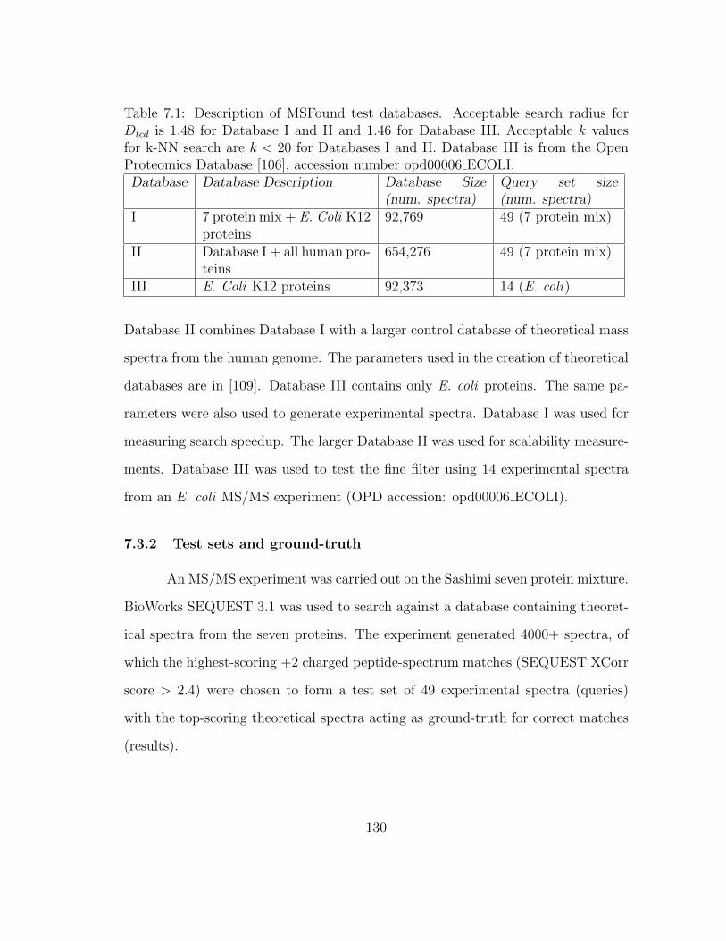
Table 7.1: Description of MSFound test databases. Acceptable search radius forDtcd is 1.48 for Database I and II and 1.46 for Database III. Acceptable k valuesfor k-NN search are k < 20 for Databases I and II. Database III is from the OpenProteomics Database [106], accession number opd00006 ECOLI.Database Database Description Database Size

(num. spectra)Query set size(num. spectra)

I 7 protein mix + E. Coli K12proteins

92,769 49 (7 protein mix)

II Database I + all human pro-teins

654,276 49 (7 protein mix)

III E. Coli K12 proteins 92,373 14 (E. coli)

Database II combines Database I with a larger control database of theoretical mass

spectra from the human genome. The parameters used in the creation of theoretical

databases are in [109]. Database III contains only E. coli proteins. The same pa-

rameters were also used to generate experimental spectra. Database I was used for

measuring search speedup. The larger Database II was used for scalability measure-

ments. Database III was used to test the fine filter using 14 experimental spectra

from an E. coli MS/MS experiment (OPD accession: opd00006 ECOLI).

7.3.2 Test sets and ground-truth

An MS/MS experiment was carried out on the Sashimi seven protein mixture.

BioWorks SEQUEST 3.1 was used to search against a database containing theoret-

ical spectra from the seven proteins. The experiment generated 4000+ spectra, of

which the highest-scoring +2 charged peptide-spectrum matches (SEQUEST XCorr

score > 2.4) were chosen to form a test set of 49 experimental spectra (queries)

with the top-scoring theoretical spectra acting as ground-truth for correct matches

(results).

130

0

2

4

6

8

10

12

14

16

18

20

0.4 0.6 0.8 1 1.2 1.4 1.6 1.8

Fre

quen

cy

Precursor mass error (theoretical Vs. experimental spectra)

abs(precursor mass difference)

Figure 7.1: Choosing precursor masstolerance τpm: A histogram of δpm, theabsolute precursor mass difference be-tween an experimental spectrum andits corresponding theoretical spectrum,shows that δpm ∈ [0,1.7] Da. We setτpm=2 Da (Equation 7.10)

0

20

40

60

80

100

1 1.1 1.2 1.3 1.4 1.5 1.6

% o

f tru

e po

sitiv

es r

etur

ned

Radius

Database IDatabase II

(a) Choosing search radius R

30

40

50

60

70

80

90

100

2 4 6 8 10 12 14 16 18 20

% o

f tru

e po

sitiv

es r

etur

ned

k in k-NN


(b) Choosing k in K-NN

Figure 7.2: We report results using the smallest values of R and k at which alltrue positives are returned for the query sets of Database I and II: R=1.48, k=3 forDatabase I, k=16 for Database II

7.4 Parameter Selection

To determine the precursor mass tolerance, τpm, we plotted a histogram of the

difference in experimental and theoretical precursor mass in spectra in our ground-

truth set (Figure 7.1). The maximum difference was ∼1.7Da, and in our experiments

we used τpm = 2.0Da. Peak mass tolerance was set to τms = 0.2Da, which is a

standard value for for the mass spectrometers used in this study.

To evaluate the index, range and k-NN searches were run against the Database

131

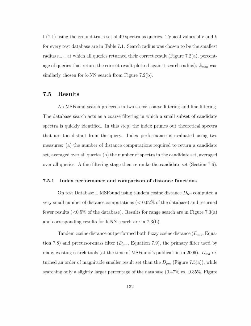
I (7.1) using the ground-truth set of 49 spectra as queries. Typical values of r and k

for every test database are in Table 7.1. Search radius was chosen to be the smallest

radius rmin at which all queries returned their correct result (Figure 7.2(a), percent-

age of queries that return the correct result plotted against search radius). kmin was

similarly chosen for k-NN search from Figure 7.2(b).

7.5 Results

An MSFound search proceeds in two steps: coarse filtering and fine filtering.

The database search acts as a coarse filtering in which a small subset of candidate

spectra is quickly identified. In this step, the index prunes out theoretical spectra

that are too distant from the query. Index performance is evaluated using two

measures: (a) the number of distance computations required to return a candidate

set, averaged over all queries (b) the number of spectra in the candidate set, averaged

over all queries. A fine-filtering stage then re-ranks the candidate set (Section 7.6).

7.5.1 Index performance and comparison of distance functions

On test Database I, MSFound using tandem cosine distance Dtcd computed a

very small number of distance computations (< 0.02% of the database) and returned

fewer results (<0.5% of the database). Results for range search are in Figure 7.3(a)

and corresponding results for k-NN search are in 7.3(b).

Tandem cosine distance outperformed both fuzzy cosine distance (Dms, Equa-

tion 7.8) and precursor-mass filter (Dpm, Equation 7.9), the primary filter used by

many existing search tools (at the time of MSFound’s publication in 2006). Dtcd re-

turned an order of magnitude smaller result set than the Dpm (Figure 7.5(a)), while

searching only a slightly larger percentage of the database (0.47% vs. 0.35%, Figure

132

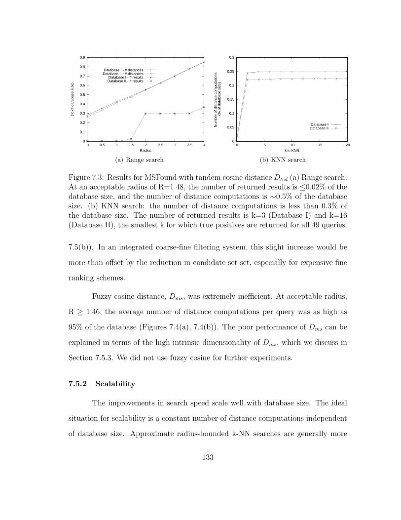
0

0.1

0.2

0.3

0.4

0.5

0.6

0.7

0.8

0.9

0 0.5 1 1.5 2 2.5 3 3.5 4

(% o

f dat

abas

e si

ze)

Radius

Database I - # distancesDatabase II - # distances

Database I - # resultsDatabase II - # results

(a) Range search

0

0.05

0.1

0.15

0.2

0.25

0.3

0 5 10 15 20

Num

ber

of d

ista

nce

com

puta

tions

(

% o

f dat

abas

e si

ze)

k in KNN


(b) KNN search

Figure 7.3: Results for MSFound with tandem cosine distance Dtcd (a) Range search:At an acceptable radius of R=1.48, the number of returned results is ≤0.02% of thedatabase size, and the number of distance computations is ∼0.5% of the databasesize. (b) KNN search: the number of distance computations is less than 0.3% ofthe database size. The number of returned results is k=3 (Database I) and k=16(Database II), the smallest k for which true positives are returned for all 49 queries.

7.5(b)). In an integrated coarse-fine filtering system, this slight increase would be

more than offset by the reduction in candidate set set, especially for expensive fine

ranking schemes.

Fuzzy cosine distance, Dms, was extremely inefficient. At acceptable radius,

R ≥ 1.46, the average number of distance computations per query was as high as

95% of the database (Figures 7.4(a), 7.4(b)). The poor performance of Dms can be

explained in terms of the high intrinsic dimensionality of Dms, which we discuss in

Section 7.5.3. We did not use fuzzy cosine for further experiments.

7.5.2 Scalability

The improvements in search speed scale well with database size. The ideal

situation for scalability is a constant number of distance computations independent

of database size. Approximate radius-bounded k-NN searches are generally more

133

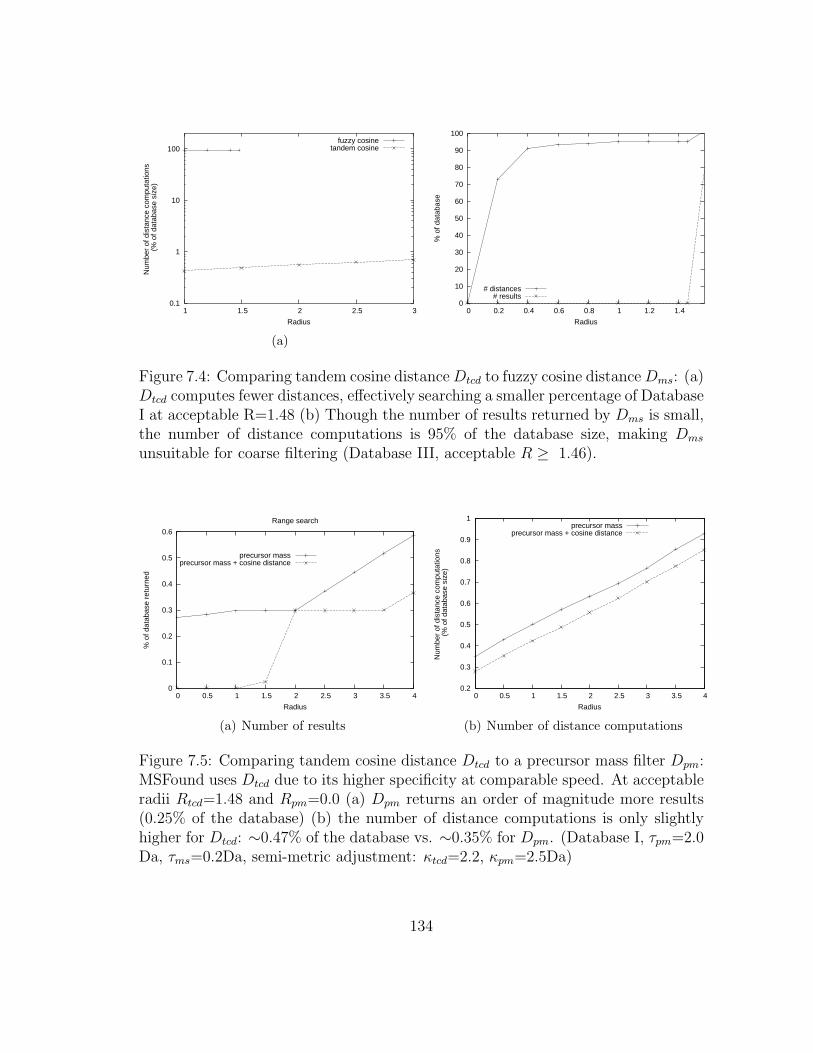
0.1

1

10

100

1 1.5 2 2.5 3

Num

ber

of d

ista

nce

com

puta

tions

(

% o

f dat

abas

e si

ze)

Radius

fuzzy cosinetandem cosine

(a)

0

10

20

30

40

50

60

70

80

90

100

0 0.2 0.4 0.6 0.8 1 1.2 1.4

% o

f dat

abas

e

Radius

# distances# results

Figure 7.4: Comparing tandem cosine distanceDtcd to fuzzy cosine distanceDms: (a)Dtcd computes fewer distances, effectively searching a smaller percentage of DatabaseI at acceptable R=1.48 (b) Though the number of results returned by Dms is small,the number of distance computations is 95% of the database size, making Dms

unsuitable for coarse filtering (Database III, acceptable R ≥ 1.46).

0

0.1

0.2

0.3

0.4

0.5

0.6

0 0.5 1 1.5 2 2.5 3 3.5 4

% o

f dat

abas

e re

turn

ed

Radius

Range search

precursor massprecursor mass + cosine distance

(a) Number of results

0.2

0.3

0.4

0.5

0.6

0.7

0.8

0.9

1

0 0.5 1 1.5 2 2.5 3 3.5 4

Num

ber

of d

ista

nce

com

puta

tions

(

% o

f dat

abas

e si

ze)

Radius

precursor massprecursor mass + cosine distance

(b) Number of distance computations

Figure 7.5: Comparing tandem cosine distance Dtcd to a precursor mass filter Dpm:MSFound uses Dtcd due to its higher specificity at comparable speed. At acceptableradii Rtcd=1.48 and Rpm=0.0 (a) Dpm returns an order of magnitude more results(0.25% of the database) (b) the number of distance computations is only slightlyhigher for Dtcd: ∼0.47% of the database vs. ∼0.35% for Dpm. (Database I, τpm=2.0Da, τms=0.2Da, semi-metric adjustment: κtcd=2.2, κpm=2.5Da)

134

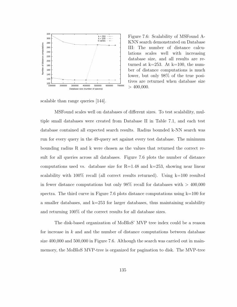
100

120

140

160

180

200

220

240

260

280

300

320

100000 200000 300000 400000 500000 600000 700000

Num

ber

of d

ista

nce

com

puta

tions

Database size (number of spectra)

k = 253k = 100k varies

Figure 7.6: Scalability of MSFound A-KNN search demonstrated on DatabaseIII: The number of distance calcu-lations scales well with increasingdatabase size, and all results are re-turned at k=253. At k=100, the num-ber of distance computations is muchlower, but only 98% of the true posi-tives are returned when database size> 400,000.

scalable than range queries [144].

MSFound scales well on databases of different sizes. To test scalability, mul-

tiple small databases were created from Database II in Table 7.1, and each test

database contained all expected search results. Radius bounded k-NN search was

run for every query in the 49-query set against every test database. The minimum

bounding radius R and k were chosen as the values that returned the correct re-

sult for all queries across all databases. Figure 7.6 plots the number of distance

computations used vs. database size for R=1.48 and k=253, showing near linear

scalability with 100% recall (all correct results returned). Using k=100 resulted

in fewer distance computations but only 98% recall for databases with > 400,000

spectra. The third curve in Figure 7.6 plots distance computations using k=100 for

a smaller databases, and k=253 for larger databases, thus maintaining scalability

and returning 100% of the correct results for all database sizes.

The disk-based organization of MoBIoS’ MVP tree index could be a reason

for increase in k and and the number of distance computations between database

size 400,000 and 500,000 in Figure 7.6. Although the search was carried out in main-

memory, the MoBIoS MVP-tree is organized for pagination to disk. The MVP-tree

135

implementation has discontinuous increases in height as the database grows, as is

commonly observed in the depth increase of B+ trees in relational databases [39].

The other possible reason is the approximate nature of the k-NN search discussed

below.

Scalability can be attributed to the version of k-NN radius bounded search

used in MoBIoS [144]. The algorithm relaxes the requirement that the k best neigh-

bors are returned first [143]. The k-1 hits are not guaranteed to be closest to the

query [144], but the first result of MoBIoS’ approximate k-NN algorithm is guaran-

teed to be the closest.

The k-NN algorithm used in this work has good scalability and accuracy in

the coarse-fine filter paradigm. Since the final top-ranked hit is determined by the

fine ranking phase, it need not be the nearest neighbor in the coarse filtering stage.

In this situation, scalable fast searches of approximate k-NN are preferred as long

as the search returns a candidate set large enough to contain the final best match

most of the time (ε-approximate k-NN). As a final note, k = 1 would be sufficient

if the fine filter’s top-hit was guaranteed to preserve the coarse-filter ordering, and

we only required the top match.

Protein identification by database search is a particularly good application

domain for approximate k-NN because of the redundancy in spectra-to-peptide

matches. Occasional incorrect PSMs have a smaller effect on protein identification

if multiple spectra usually match to a given peptide, and only the highest scoring

PSM contributes to the protein score (ProteinProphet, Equation 2.2). A direction

for future work would be to test the extent to which approximate spectrum match-

ing affects the accuracy of recently developed approaches to quantitative proteomics

where spectral counts are used to estimated protein abundance (Chapter 8).

136

7.5.3 Intrinsic dimensionality as an indicator of search performance

The performance of search using space-partitioning methods depends on the

dimensionality of the search space. The concept of dimensionality must be redefined

for metric spaces since points are not restricted to a vector or coordinate space.

Instead, a metric space is characterized by the distribution of pairwise distances.

This leads to the definition of the intrinsic dimensionality ρ of a search space.

The most well-known definition of ρ is due to Chavez and Navarro, who defined

ρ = µ2/2σ2 using the mean µ and variance σ2 of a distribution of pair-wise distances

[12].

The difference in performance between tandem cosine distance Dtcd and fuzzy

cosine distance Dms can be explained in terms of the intrinsic dimensionality of the

two spaces. A histogram of pair-wise distances that peaks at large distance values

is indicative of high ρ. Dtcd has a well-behaved histogram of pair-wise distances

(Figure 7.7), as opposed to Dms which has a highly peaked histogram.

The precursor mass difference term, Dpm, in Dtcd (Equation 7.10) acts to

reduce the intrinsic dimensionality of the Dtcd search space, by effectively filtering

on a single dimension, before the cosine distance component kicks in. We confirmed

this reduction in ρ empirically using a different definition of ρ introduced by Mao et

al, who define ρq based on application queries, as the slope coefficient α of a linear

regression log(n) = αlog(r) + β, where n is the number of results returned by a

radius search of radius r [82]. We estimated ρq ∼ 1 for range queries using tandem

cosine distance Dtcd.

Performance of nearest-neighbor searches degrades to a linear scan in high

dimensions [120]. Intuitively, this is because at higher dimensions points are almost

137

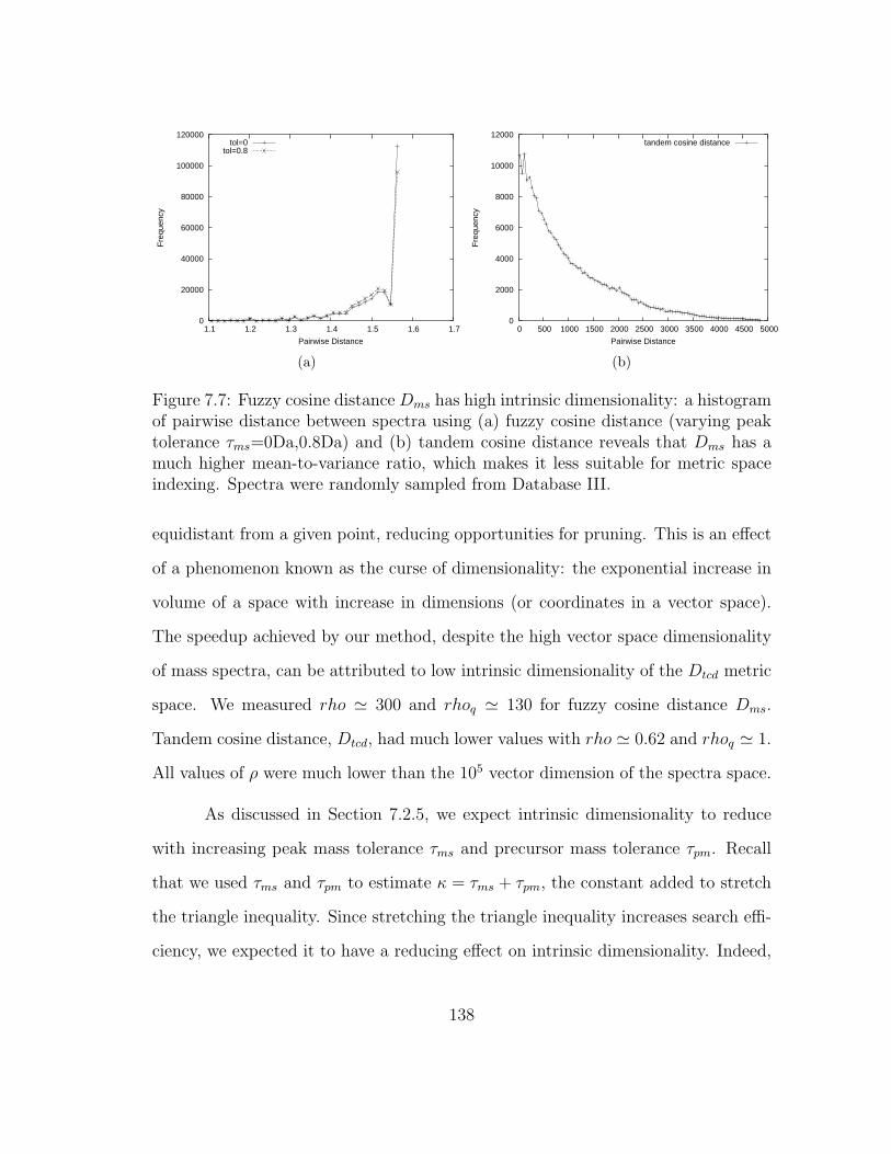
0

20000

40000

60000

80000

100000

120000

1.1 1.2 1.3 1.4 1.5 1.6 1.7

Fre

quen

cy

Pairwise Distance

tol=0tol=0.8

(a)

0

2000

4000

6000

8000

10000

12000

0 500 1000 1500 2000 2500 3000 3500 4000 4500 5000

Fre

quen

cy

Pairwise Distance

tandem cosine distance

(b)

Figure 7.7: Fuzzy cosine distance Dms has high intrinsic dimensionality: a histogramof pairwise distance between spectra using (a) fuzzy cosine distance (varying peaktolerance τms=0Da,0.8Da) and (b) tandem cosine distance reveals that Dms has amuch higher mean-to-variance ratio, which makes it less suitable for metric spaceindexing. Spectra were randomly sampled from Database III.

equidistant from a given point, reducing opportunities for pruning. This is an effect

of a phenomenon known as the curse of dimensionality: the exponential increase in

volume of a space with increase in dimensions (or coordinates in a vector space).

The speedup achieved by our method, despite the high vector space dimensionality

of mass spectra, can be attributed to low intrinsic dimensionality of the Dtcd metric

space. We measured rho ' 300 and rhoq ' 130 for fuzzy cosine distance Dms.

Tandem cosine distance, Dtcd, had much lower values with rho ' 0.62 and rhoq ' 1.

All values of ρ were much lower than the 105 vector dimension of the spectra space.

As discussed in Section 7.2.5, we expect intrinsic dimensionality to reduce

with increasing peak mass tolerance τms and precursor mass tolerance τpm. Recall

that we used τms and τpm to estimate κ = τms + τpm, the constant added to stretch

the triangle inequality. Since stretching the triangle inequality increases search effi-

ciency, we expected it to have a reducing effect on intrinsic dimensionality. Indeed,

138

we measured decreasing intrinsic dimensionality with increasing τms: ρ ' 579 for

τms=0 Da, ρ ' 445 for τms=0.2 Da and ρ ' 176 for τms=2.2 Da (fuzzy cosine dis-

tance, distance distributions not shown, spectra randomly sampled from Database

III).

7.6 Fine filtering

To demonstrate a fine ranking stage, we extended a popular Bayesian score

(ProFound, [151]) for matching peptide mass fingerprinting (PMF) spectra to be

applicable to the MS/MS domain. ProFound outperformed other PMF matching

schemes in an empirical study [11]. Following ProFound’s terminology, we let k

denote the hypothesis that ’protein k is present in the sample’. ProFound computes

a posterior probability that k is present in the sample based on mass spectrum

matching data D and background information I. The likelihood P (D|kI) is modeled

as in Equation 7.12, explained below. The posterior probability is computed via

Bayes rule (Equation 7.13) using a uniform prior for all proteins P (k|I), followed

by a normalization step over the entire database.

P (D|kI) =(N − r)!N !

× (7.12)

r∏i=1

{√2

π

mmax −mmin

σi

gi∑j=1

exp

[−(mi −mij0)2

2σ2i

]}P (k|DI) ∝ P (k|I)P (D|kI) (7.13)

database∑k=1

P (k|DI) = 1 (7.14)

ProFound models every peak in a PMF spectrum as either hits or misses. Every

peak in the experimental spectrum that can be matched to at least one theoretical

peak in k’s spectrum is called a hit. Two peaks that differ by ≤ τpmDa constitute

139

a match. Random peak matches are not modeled, every hit is attributed to a

real peptide in protein k. Every experimental peak that is not a hit, is a miss. The

difference in mass between a matched experimental and theoretical peaks is modeled

as a Gaussian error, leading to the exponential term in Equation 7.12).

Of N total peptides in protein k, r is the number of hits, and w = N − r

is the number of misses. J of the w misses are modeled as coming from modified

peptides, and the rest are considered to result from other sequence or digestion errors

and are not explicitly modeled. The uniform probability mmax−mmin term models

the J ∈ [1, w] modified peptides. Derivation details are in the ProFound paper’s

supplement. In Equation 7.12, N is the total number of peptide peaks in protein

k, r is the number of peak hits, mmax and mmin are the minimum and maximum

possible masses in the database, gi is the number of peaks in k’s spectrum that

match the ith experimental peak hit, and mi and mij0 are the peak masses of those

respective matching experimental and theoretical peaks. ProFound allows only one

of multiple hits per experimental peak to be the right match (summation over gi).

Since ProFound matches two protein spectra, and we need to match two pep-

tide spectra, we simply translate the terms in Equation 7.16 to their MS/MS equiv-

alents. Peptide fragment masses are denoted by the f superscript (f=fragment), to

distinguish them from the peptide masses in ProFound’s original Equation 7.12. In

Equation 7.16, kf is a theoretical peptide with Nf fragmentation peaks, rf of which

are hits (±τms of an experimental peak). Since we are modeling PFF spectra, we

add a Gaussian error term for the precursor mass difference between experimental

(mq) and theoretical (mk) peptide masses. All other assumptions remain the same.

The posterior probability is calculated using a uniform P (kf |I) prior as before, but

normalized over the candidate set of peptide-spectrum matches returned by the

140

coarse-filter. The new equation for MS/MS spectra-matching is:

P (Df |kfI) = exp

[−(mq −mk)

2

2σ2k

]× (Nf − rf )!

Nf !× (7.15)

rf∏i=1

√

2

π

mfmax −m

fmin

σfi×

gfi∑

j=1

exp

[−

(mfi −m

fij0)2

(√

2σfi )2

]PSM candidates∑

k=1

P (kf |DfI) = 1 (7.16)

7.6.1 Results

A range search coarse filter first generated a candidate result set for each of

the 14 queries in Database III, using τpm=2.0Da, τms=0.2Da and charge state=+1.

The fine-filter then ranked the candidate set, and reported the top-scoring spectrum

as the correct result.

The ground-truth consisted of the top hit from TurboSEQUEST [146] for

each query in a set of 14 E. coli peptide fragmentation spectra searched against the

E. coli K12 genome (Database III in Table 7.1). This top result was expected to

be correct because it also generated high peptide and protein probabilities from the

TransProteomic Pipeline.

The coarse filter returned the correct result for eleven of fourteen queries

using r1.46. The remaining 3 spectra were found at higher search radius r = 3.81,

because they had precursor mass that varied from the correct theoretical spectrum

by (2.0, 2.4)Da. In any case, even when using higher radius r=3.81 for all queries, the

coarse filter returned only ∼[50,250] candidate spectra per query, while computing

distance calculations for <0.2% of the database.

The fine filter was extremely effective in finding the correct top-hit. It ranked

141

the correct result as the top-hit for all fourteen queries, with identification proba-

bility >0.99. The second ranked hit’s probability was several orders of magnitude

lower, suggesting extremely confident top-hit identification (8-15 orders of magni-

tude for thirteen queries and three orders of magnitude for the fourteenth query).

7.7 Discussion

7.7.1 Other distance metrics: Hamming Distance

As discussed in Section 7.2.3, we also tested a data representation using

coarse-resolution Boolean vectors and a Hamming distance metric. This data repre-

sentation and distance metric were outperformed by MSFound, and are summarized

here for completeness.

Given a mass range [M1, M2] Da and peak resolution Mres, MSFound uses

high-resolution Boolean vectors with N = (M1−M2)/Mres elements. These Boolean

vectors can be shrunk into coarse resolution vectors V using windows that overlap

by WDa. Here, |V | = round((N+0.5)/W ), and vi = 1 if ∃ a peak in the ith window.

For example, if M1 = 1.0 Da, Mres = 10.0 Da, and W = 5.0 Da, the windows would

be [1, 10], [6, 15], [11, 20] and so on. By this definition, vi and vi+1 could both = 1

if a peak exists in the overlap region. The overlap prevents potential mismatches

between experimental and theoretical spectra due to peak shifts in experimental

spectra at window edges. The overlap parameter W must be chosen to balance false

positives and false negatives.

Hamming distance can be used to compare two coarse resolution vectors V1

and V2, and is defined as the cardinality of XOR(V1, V2). It counts the number of

mismatched peaks, and is a metric.

142

0

10

20

30

40

50

60

70

80

90

100

0 20 40 60 80 100 120

Num

ber

of d

ista

nces

(%

of d

atab

ase

size

)

Radius

w10 (R=120)w20 (R=57)w40 (R=33)w80 (R=13)

w100 (R=10)w160 (R=6)w240 (R=4)

(a) Number of distance computations

0

10

20

30

40

50

60

70

0 20 40 60 80 100 120

Num

ber

of r

esul

ts (

% o

f dat

abas

e si

ze)

Radius

w10 (R=120)w20 (R=57)w40 (R=33)w80 (R=13)

w100 (R=10)w160 (R=6)w240 (R=4)

(b) Number of results

Figure 7.8: Evaluating Hamming distance and low-resolution spectrum representa-tion at different window sizes W: Hamming distance has low specificity as a coarsefilter (compare against Dms in Figure 7.4(b)). R is the acceptable search radius atwhich all true positives are returned (Database III)

Increasing window (W) size produced smaller dimensional vectors (coarser

resolutions) and reduced the number of distance computations (Figure 7.8(a)), since

indexing lower dimensional vectors is an easier problem. However, increasing W also

increases the probability of a random hit, so the number of false positive results in-

crease with W (Figure 7.8(b)). Note that an acceptable radius R must be determined

for every W .

7.7.2 Charge state

Experimental spectrum peaks are mass-to-charge (m/z) ratios. The precursor

peak is charged, and the fragments might also pick up positive charge, but this

phenomenon is not deterministic, and the spectrum could contain either +1 or +z

charged peaks or both. In our experiments, storing theoretical spectra with multiply

charged fragments was not useful. Charged fragments did not significantly increase

performance, used 2-3 times more disk space, and increased the chance of a random

143

match.

MSFound used a simple heuristic based on the maximum m/z peak to esti-

mate if the precursor charge state is z = 1 or z = 2, 3. In general, we store only

+1 charged spectra in the theoretical database, and assume a preprocessing step

that estimates the charge state of the query spectrum [65] and adjusts the precursor

mass accordingly. The precursor mass of a +z charged experimental spectrum can

be computed as x = qz − z, where q is the measured m/z.

7.8 Related work

7.8.1 Hash-based indexing

Recently, Dutta and Chen [29] applied another metric-space indexing tech-

nique, Locality Sensitive Hashing (LSH), to mass spectra searches. The LSH algo-

rithm [42] is an efficient hash-based indexing structure for nearest neighbor searches,

that also provides elegant probabilistic bounds on the error of the returned re-

sults [121].

LSH is a randomized algorithm that can be used to solve exact and approxi-

mate near neighbor problems (in computational theory, the near neighbor problem

is the decision version of the nearest neighbor problem). LSH relies on the availabil-

ity of locality-sensitive hash functions. Locality sensitive implies that if two points

are within distance r1 from each other, they will hash to the same value (collision)

with probability ≥ p1, and if they are greater than a distance r2 apart, they will

collide with probability ≤ p2. For the ε-A-KNN problem, r2 = r1(1 + ε). Multiple

hash functions are used to separate the gap between p1 and p2. Once a database

has been hashed using LSH, the near neighbors can be determined by hashing the

query point and retrieving elements stored in the hash bucket containing the query

144

point [121]. LSH retrieval can result in sub-linear query time for certain families

of hash functions and distance metrics e.g. Indyk and Motwani construct a family

of hash functions that results in time complexity O(nρ), ρ = 1/ε if the L1 norm is

used [50], Datar et al [23] extend this result to the Ls norm, s ∈ (0, 2], and more

recently Jain et al [51] show the existence of hash functions using Mahalanobis

distances.

Dutta and Chen embedded spectra into a vector space, by discretizing the

mass range [M1,M2]into x = 2Da intervals. They added a peak-intensity based pre-

processing step to filter out noisy peaks from experimental spectra. This cleaning

step increased accuracy of matching and reduced vector dimension. Then they ap-

plied LSH to index theoretical spectra vectors and ran range queries using Euclidean

distance. They measured speedup by comparing the number of results returned by

their method to the total number of peptides within a precursor mass ±∆ of the

query (comparison against Dpm as in Section 7.5). LSH reduced the number of

returned candidate peptides by one or two orders of magnitude, depending on the

dimension of the spectra vectors, with <1% incorrect matches. However, the paper

did not compare results against MSFound, and was evaluated on different datasets.

7.8.2 Clustering experimental spectra to achieve speedup

Frank et al [37] adopted a different approach. Instead of tackling the prob-

lem at the database search end, they achieved speedup by reducing the number

of queries. Every MS/MS experiment produces tens of thousands of experimental

spectra; each one is queried against the database. They clustered all experimental

spectra using a greedy version of hierarchical agglomerative clustering (HAC), and

chose the cluster representatives as queries. The approach was approximate since

145

their HAC variant did not merge the best clusters at each step, and greedily merged

adjacent clusters that satisfied an empirical similarity threshold, with decreasing

thresholds at each level. A number of other heuristics were used to speedup the

distance computation. Their data representation step also relied on a number of

heuristics e.g. choosing a subset of best peaks per spectrum (highest-intensity 15

peaks per 1000 Da), or peak intensity scaling (scale intensities to 1000, and then

log-transform). There was no explanation for these parameter choices.

With all the heuristic optimizations in place, the approach achieved similar

speedups to both MSFound and LSH [37], suggesting that a combination of exper-

imental spectra clustering and database indexing should result in higher speedups

than either approach alone.

7.8.3 Detecting post-translational modifications

Detecting PTMs efficiently is one of the largest challenges in computational

MS/MS peptide identification. The problem is hard because a post-translational

modification in a peptide causes an increase (or decrease) in peptide mass mass,

as well as a mass shift on every fragment that contains the modified amino-acid,

completely changing the spectrum peak list. The problem is compounded by the ex-

istence of 200+ known modifications [43] and possibly more unknown ones. Further,

a peptide can be the target of multiple PTMs, and since PTMs are dynamic, we can

expect to find both modified and unmodified versions of the peptide in a sample. A

final challenge is to also locate the PTM site (which amino-acid is modified).

PTM-specific scoring metrics are computationally more expensive than the

Euclidean distance used in LSH or tandem cosine distance used in MSFound. One of

the first computational solutions to detecting PTMs used a dynamic programming

146

(DP) to detect a predefined number of modifications per spectrum, by counting sim-

ilar peaks within a band along the diagonal of the DP matrix [102]. This method

is similar to dynamic time warping methods used in speech recognition [116], where

two equivalent speech signals can be mutually shifted due to different speech speeds.

The disadvantage of dynamic programming is that it is slow, with O(n2) time com-

plexity.

The authors have since extended the dynamic programming concept by adding

a database filtering step [131], into a tool called Inspect, which uses a combination of

de-novo and in-silico methods to detect PTMs. Tanner et al first use local de-novo

sequencing to detect small peptide sequences (tags) from an experimental spectrum.

Then they filter the theoretical database to generate a candidate set of peptides con-

taining the sequence tags, using a trie [2] index for fast string matching. A dynamic

programming technique is used to detect any modifications on the candidate pep-

tides, which are then finally ranked using a probabilistic model to compute the

likelihood of the peptide-spectrum match.

In theory, coarse filtering approaches like MSFound should be able to de-

tect PTM-based peak shifts by setting peak-tolerance parameters appropriately. In

practice, this approach will at best detect one or two types of modifications, before

being overwhelmed by false positive matches. Dutta and Chen also indicated that

their LSH method may be suitable for detecting PTMs since their distance metric

does not consider precursor mass. They illustrated their point with a few examples,

but did not provide any specific methodology or results.

147

Chapter 8

Conclusions and Future Directions

8.1 Contributions

Over the past decade, research in proteomics has focused on developing in-

creasingly sensitive mass spectrometers and better computational and statistical

methods to interpret spectral data. However, inadequate coverage and repeatability

of MS/MS experiments [130] are roadblocks to widespread biomarker discovery via

proteomics [75].

In tandem with the proteomics revolution, advances in systems biology have

resulted in genome-wide characterization of gene/protein function and interactions.

This dissertation showed that closing the loop between computational proteomics

and systems biology is an attractive and feasible approach to improving MS/MS

based protein identification. We introduced the predictive modeling methods that

are typical of systems biology studies into the proteomic data analysis pipeline. This

research involved using relevant knowledge from outside the proteomics experiment

as prior evidence of protein presence, bringing both single gene data and gene-gene

dependency data into protein identification scores. These integrative approaches

improved protein identification rates by up to 30% as demonstrated across yeast, E.

coli and human samples (Chapters 4-6).

148

8.1.1 A systemic, integrative approach to computational proteomics

MSNet (Chapters 5-6) is a first step towards our larger vision for the pro-

teomics field: to (a) enable systemic approaches for the analysis of proteomics exper-

iments in which (b) identified proteins are immediately interpretable in the context

of their functional roles. MSNet tackled the status quo inter-protein independence

assumption made by MS/MS analysis tools. This statistical simplification rarely

holds for real data since proteins are team players and almost always act in tandem.

MSNet was implemented as a fast, iterative algorithm with an analytical solution,

and hence a proof of convergence for connected graphs. Chapter 5 showed that the

MSNet algorithm had strong ties to a personalized variant of PageRank, a random

walk algorithm used by the Google search engine to rank web pages based on hyper-

link structure and query topic. Chapter 6 discussed MSNet’s ties with the Markov

Random Field framework. MSNet easily scales to mammalian proteomes containing

tens of thousands of proteins.

The second contribution, MSPresso (Chapter 4), was motivated by the facts

that both gene and protein expression are both required to understand cellular pro-

cesses [25], and that currently measurement of large-scale gene expression levels

is a more mature technology today than measurement of protein expression [77].

MSPresso learned a genome-wide logistic relationship between mRNA concentra-

tion and MS/MS-based protein detection, and estimated a more accurate posterior

probability of protein presence given both mRNA and MS/MS data. Incorporat-

ing observed mRNA evidence into the statistical analysis of an MS/MS experiment

provided a far more complete snapshot of protein presence: MSPresso probabilities

increased area under ROC curves by as much as 20% when evaluated against protein

benchmarking datasets. We also showed applicability of MSPresso in cases where

149

matching high-quality mRNA data was not available.

8.1.2 Database indexing framework for peptide spectrum matching

The third contribution addressed a core algorithmic issue concerning the ex-

ecution speed and scalability of MS/MS protein identification by database lookup.

Analysis of MS/MS experiments involves matching several thousand MS/MS spec-

tra to known peptide sequences in large databases. Exact searches are not effective

since experimental spectra differ from expected signatures due to the semi-stochastic

sampling in the instrument, noise, or dynamic chemical modifications. Chapter 7 de-

scribed an effective distance function for matching noisy, high-dimensional MS/MS

spectra that resulted in very fast database searches when used with a scalable k-

nearest neighbor search algorithm and a metric-space database index tree data struc-

ture (MoBIoS). MSFound achieved an order of magnitude speedup over prevalent

search techniques, while maintaining scalability to large peptide spectra databases.

To our knowledge, MSFound was the first effort to formulate database indexing se-

mantics for MS/MS peptide spectra. This dissertation analyzed MSFound’s speedup

in terms of the intrinsic dimensionality of the search space, a well-founded paradigm

for studying approximate search of high-dimensional, sparse datasets [12].

8.1.3 Benchmarking and evaluation

Finally, this dissertation presented comprehensive benchmarking datasets for

computational proteomics in yeast. We believe that the availability of these reference

sets will assist algorithmic advances in the field, much as the significant effort spent

designing these benchmarks for MSPresso streamlined the evaluation of MSNet.

150

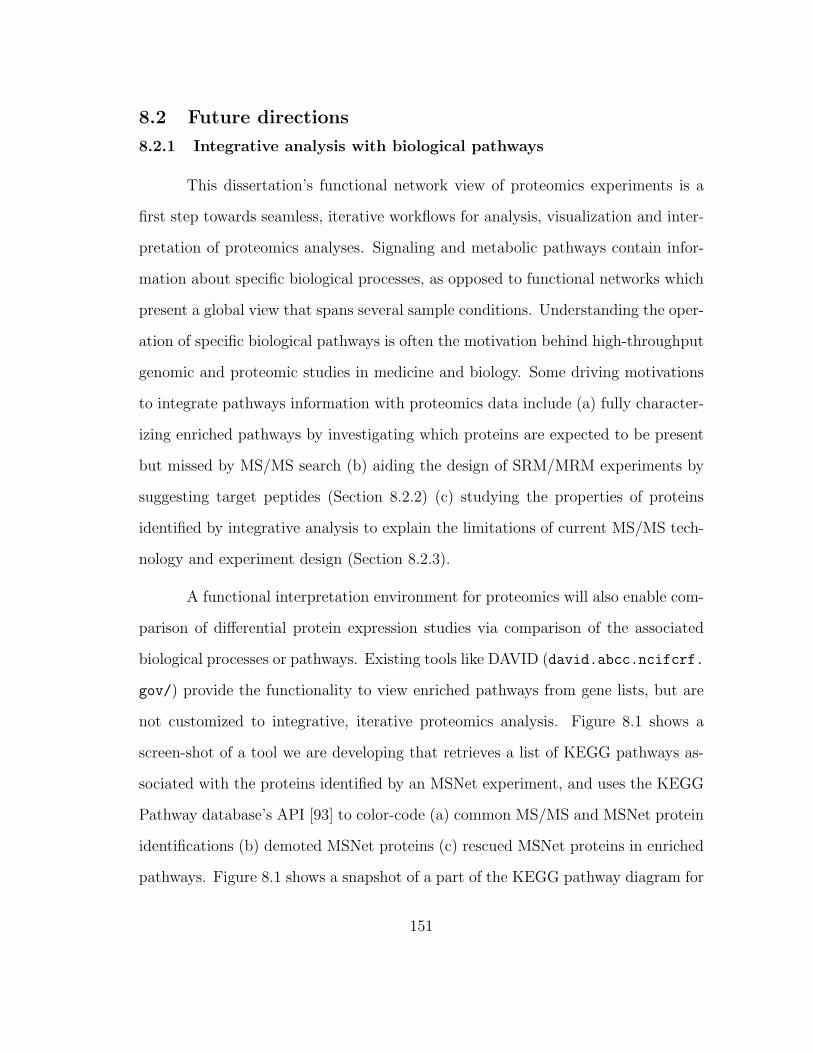
8.2 Future directions

8.2.1 Integrative analysis with biological pathways

This dissertation’s functional network view of proteomics experiments is a

first step towards seamless, iterative workflows for analysis, visualization and inter-

pretation of proteomics analyses. Signaling and metabolic pathways contain infor-

mation about specific biological processes, as opposed to functional networks which

present a global view that spans several sample conditions. Understanding the oper-

ation of specific biological pathways is often the motivation behind high-throughput

genomic and proteomic studies in medicine and biology. Some driving motivations

to integrate pathways information with proteomics data include (a) fully character-

izing enriched pathways by investigating which proteins are expected to be present

but missed by MS/MS search (b) aiding the design of SRM/MRM experiments by

suggesting target peptides (Section 8.2.2) (c) studying the properties of proteins

identified by integrative analysis to explain the limitations of current MS/MS tech-

nology and experiment design (Section 8.2.3).

A functional interpretation environment for proteomics will also enable com-

parison of differential protein expression studies via comparison of the associated

biological processes or pathways. Existing tools like DAVID (david.abcc.ncifcrf.

gov/) provide the functionality to view enriched pathways from gene lists, but are

not customized to integrative, iterative proteomics analysis. Figure 8.1 shows a

screen-shot of a tool we are developing that retrieves a list of KEGG pathways as-

sociated with the proteins identified by an MSNet experiment, and uses the KEGG

Pathway database’s API [93] to color-code (a) common MS/MS and MSNet protein

identifications (b) demoted MSNet proteins (c) rescued MSNet proteins in enriched

pathways. Figure 8.1 shows a snapshot of a part of the KEGG pathway diagram for

151

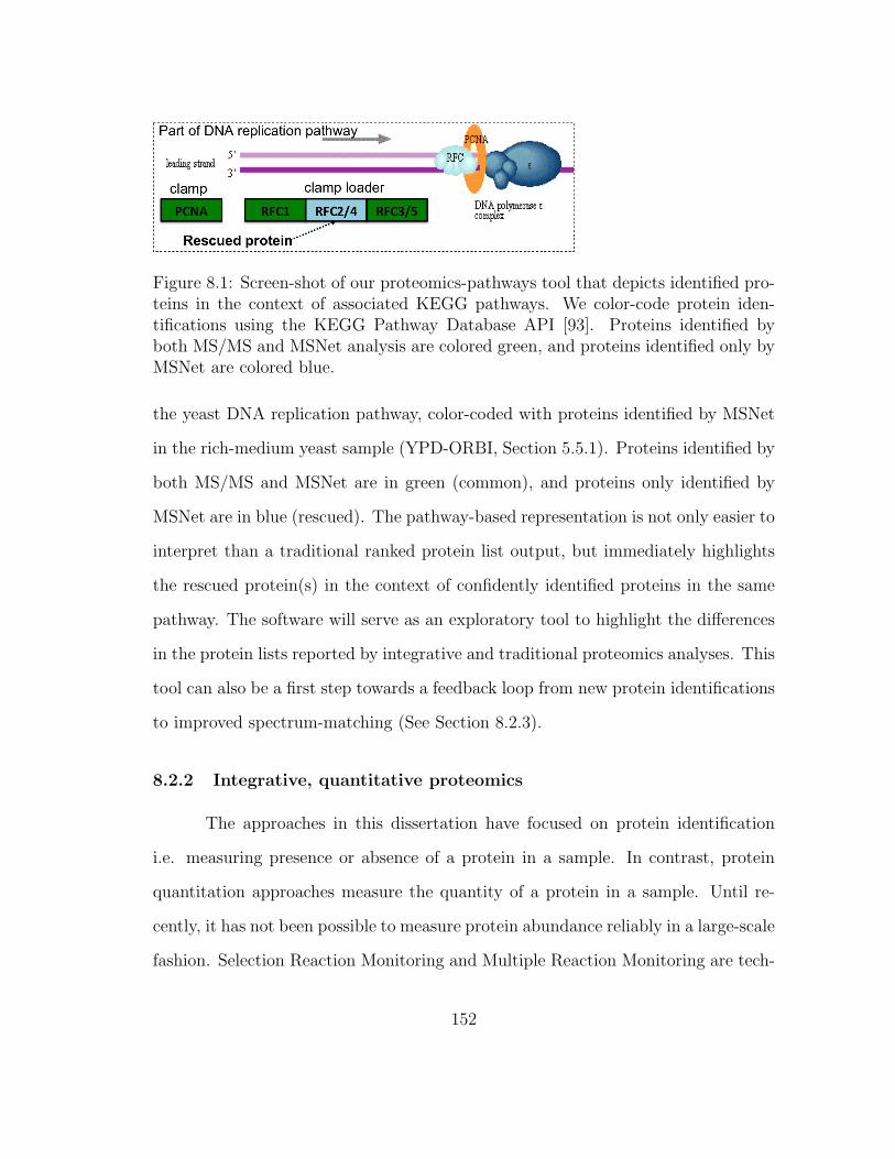
Figure 8.1: Screen-shot of our proteomics-pathways tool that depicts identified pro-teins in the context of associated KEGG pathways. We color-code protein iden-tifications using the KEGG Pathway Database API [93]. Proteins identified byboth MS/MS and MSNet analysis are colored green, and proteins identified only byMSNet are colored blue.

the yeast DNA replication pathway, color-coded with proteins identified by MSNet

in the rich-medium yeast sample (YPD-ORBI, Section 5.5.1). Proteins identified by

both MS/MS and MSNet are in green (common), and proteins only identified by

MSNet are in blue (rescued). The pathway-based representation is not only easier to

interpret than a traditional ranked protein list output, but immediately highlights

the rescued protein(s) in the context of confidently identified proteins in the same

pathway. The software will serve as an exploratory tool to highlight the differences

in the protein lists reported by integrative and traditional proteomics analyses. This

tool can also be a first step towards a feedback loop from new protein identifications

to improved spectrum-matching (See Section 8.2.3).

8.2.2 Integrative, quantitative proteomics

The approaches in this dissertation have focused on protein identification

i.e. measuring presence or absence of a protein in a sample. In contrast, protein

quantitation approaches measure the quantity of a protein in a sample. Until re-

cently, it has not been possible to measure protein abundance reliably in a large-scale

fashion. Selection Reaction Monitoring and Multiple Reaction Monitoring are tech-

152

niques that can be used to analyze targeted peptides, and absolute abundance is

measured by calibrating the signal intensity of a peptide against a reference pep-

tide isotope of known abundance. These approaches are more labor-intensive, but

highly sensitive and reproducible. Vogel and Marcotte [135] survey recent advances

in computational alternatives that aim to directly estimate absolute protein abun-

dance from shotgun mass spectrometry experiments e.g. using spectral or peptide

counts [77], peak intensities [124], or both [78]. Measuring protein abundance is

of extreme value in understanding cellular machinery since biological processes and

pathways are often driven by up-regulation or down-regulation of proteins.

Future directions include modeling the relationship between protein degrada-

tion and mRNA degradation rates [25] from libraries of gene and protein expression

data, and enabling integrative, quantitative proteomics analyses using estimated

protein abundances in tandem with pathways enriched for identified proteins.

A functional link in the gene functional networks used in this dissertation [70]

need not necessarily imply similar quantitation profiles since the network was gen-

erated from diverse genomic datasets including phylogenetic profiles and literature

co-citation counts for genes. A future direction is to investigate more targeted data

sources such as protein-protein interaction networks for integrative analysis at the

protein identification and quantitation levels.

8.2.3 Knowledge-based detection of post-translationally modified pep-tides

Peptide-spectrum matching studies are poised to increasingly leverage a com-

bination of de novo and database lookup algorithms to identify splice variants (iso-

forms) and PTMs [131]. A useful next step would to close the feedback loop be-

153

tween the integrative protein-level approaches of this dissertation and the peptide-

spectrum matching approaches at the beginning of the MS/MS pipeline. A large

percentage of spectra in a proteomics experiment go unmapped to real peptides, thus

reducing the percent of a protein sequence that is identified [100]. The unmapped

peptides of proteins identified by integrative analysis could be used as a starting

point to improve sequence coverage. A rule-based system that accesses knowledge

bases of known PTMs, splice variants and SNAPs (single modified amino acid) [4,20]

could be used to explain why these peptides initially went unidentified. For instance,

a rule-based, targeted, spectrum-matching step could avoid the computational in-

feasibility of blind PTM searches by using prior knowledge of which PTMs to expect

in a given set of peptides. For such approaches to be feasible, current knowledge-

bases must be organized and annotated to allow retrieval of facts relevant to a given

sample - a challenge that is both computational and social.

8.2.4 Consensus across multiple high-throughput proteomics experiments

In Chapter 3, we tested several notions of combining reference proteomics

experiments into a benchmark set, primarily using expert knowledge to up-weight

identifications from trusted experiments, or using expectation-maximization clus-

tering. Clusters that span different spaces of the proteome could hold insight about

proteins that are only detectable by certain technologies.

Consensus clustering is a general paradigm for situations where a number

of different input clusterings have been obtained and we require a single consensus

clustering which is a ‘better’ fit, without necessarily accessing the individual protein

features used by each input clustering [108,127]. The benchmarking set problem can

be framed as a consensus clustering problem, where each high-throughput reference

154

experiment itself produces two clusters of proteins: ‘present’ and ‘absent’. Though

cluster evaluation is generally non-trivial and domain-dependent, the consensus clus-

ters could be evaluated against the hand-crafted benchmarking sets described in this

dissertation as a starting point.

A larger application of consensus clustering arises due to the low experi-

ment coverage and repeatability typical of MS/MS proteomics experiments [130].

Different technologies and analysis platforms produce different, overlapping lists of

identifications from the same sample. There is a need for algorithms that consoli-

date results from different data analysis platforms, instruments, runs or laboratories

without necessarily having access to the individual features that went into the design

of each experiment.

155

Bibliography

[1] The official google blog, 2008. http://googleblog.blogspot.com/2008/07/we-

knew-web-was-big.html.

[2] A. V. Aho and M. J. Corasick. Efficient string matching: an aid to biblio-

graphic search. Commun. ACM, 18(6):333–340, June 1975.

[3] T. E. Allen, M. J. Herrgard, M. Liu, Y. Qiu, J. D. Glasner, F. R. Blattner,

and B. O. Palsson. Genome-scale analysis of the uses of the escherichia

coli genome: Model-driven analysis of heterogeneous data sets. J Bacteriol,

185(21):6392–9, 2003.

[4] R. Apweiler, A. Bairoch, C. H. Wu, W. C. Barker, B. Boeckmann, S. Ferro,

E. Gasteiger, H. Huang, R. Lopez, M. Magrane, M. J. Martin, D. A. Natale,

C. O’Donovan, N. Redaschi, and L.-S. L. Yeh. Uniprot: the universal protein

knowledgebase. Nucleic Acids Res, 32(Database issue):D115–9, 2004.

[5] Y. Benjamini and Y. Hochberg. Controlling the false discovery rate: A practi-

cal and powerful approach to multiple testing. J Royal Stat Soc B, 57:289–300,

1995.

[6] J. L. Bentley. Multidimensional binary search trees used for associative

searching. Commun. ACM, 18(9):509–517, September 1975.

[7] A. Berman and R. J. Plemmons. Nonnegative matrices in the mathematical

sciences. Society for Industrial Mathematics (SIAM), 1994.

[8] G. F. Berriz, O. D. King, B. Bryant, C. Sander, and F. P. Roth. Character-

izing gene sets with funcassociate. Bioinformatics, 19(18):2502–4, 2003.

[9] J. Besag and C. Kooperberg. On conditional and intrinsic autoregressions.

Biometrika, 82(4):733–746, December 1995.

[10] T. Bozkaya and M. Ozsoyoglu. Distance-based indexing for high-dimensional

metric spaces. In ACM SIGMOD, pages 357–368. ACM Press, 1997.

156

[11] D. Chamrad, G. Korting, K. Stuhler, H. Meyer, J. Klose, and M. Bluggel.

Evaluation of algorithms for protein identification from sequence databases

using mass spectrometry data. Proteomics, 4(3):619–628, 2004.

[12] E. Chavez and G. Navarro. A probabilistic spell for the curse of dimension-

ality. In ALENEX: International Workshop on Algorithm Engineering and

Experimentation, LNCS, 2001.

[13] A. Chi, C. Huttenhower, L. Y. Geer, J. J. Coon, J. E. Syka, D. L. Bai, J. Sha-

banowitz, D. J. Burke, O. G. Troyanskaya, and D. F. Hunt. Analysis of

phosphorylation sites on proteins from saccharomyces cerevisiae by electron

transfer dissociation (etd) mass spectrometry. Proc Natl Acad Sci U S A,

104(7):2193–8, 2007.

[14] H. Choi, D. Ghosh, and A. I. Nesvizhskii. Statistical validation of peptide

identifications in large-scale proteomics using the target-decoy database search

strategy and flexible mixture modeling. J Proteome Res, 7(1):286–92, 2008.

[15] H. Choi and A. I. Nesvizhskii. False discovery rates and related statistical

concepts in mass spectrometry-based proteomics. J Proteome Res, 7(1):47–

50, 2008.

[16] J. Colinge, A. Masselot, M. Giron, T. Dessingy, and J. Magnin. OLAV: to-

wards high-throughput tandem mass spectrometry data identification. Pro-

teomics, 3:1454–63, August 2003.

[17] R. W. Corbin, O. Paliy, F. Yang, J. Shabanowitz, M. Platt, J. Lyons, C. E.,

K. Root, J. McAuliffe, M. I. Jordan, S. Kustu, E. Soupene, and D. F. Hunt.

Toward a protein profile of escherichia coli: Comparison to its transcription

profile. Proc Natl Acad Sci U S A, 100(16):9232–7, 2003.

[18] M. W. Covert, E. M. Knight, J. L. Reed, M. J. Herrgard, and B. O. Palsson.

Integrating high-throughput and computational data elucidates bacterial net-

works. Nature, 429(6987):92–6, 2004.

[19] R. Craig and R. C. Beavis. Tandem: Matching proteins with tandem mass

spectra. Bioinformatics, 20(9):1466–7, 2004.

[20] D. M. Creasy and J. S. Cottrell. Unimod: Protein modifications for mass

spectrometry. Proteomics, 4(6):1534–1536, 2004.

157

[21] P. Dagum and R. M. Chavez. Approximating probabilistic inference in

bayesian belief networks. IEEE Transactions on Pattern Analysis and Ma-

chine Intelligence, 15(3):246–255, March 1993.

[22] R. M. Daniel P. Miranker, Weijia Xu. Mobios: a metric-space dbms to support

biological discovery. In SSDBM, page 241, 2003.

[23] M. Datar, N. Immorlica, P. Indyk, and V. S. Mirrokni. Locality-sensitive

hashing scheme based on p-stable distributions. In SCG ’04: Proceedings of

the twentieth annual symposium on Computational geometry, pages 253–262,

New York, NY, USA, 2004. ACM Press.

[24] L. M. de Godoy, J. V. Olsen, G. A. de Souza, G. Li, P. Mortensen, and

M. Mann. Status of complete proteome analysis by mass spectrometry: Silac

labeled yeast as a model system. Genome Biol, 7(6):R50, 2006.

[25] R. de Sousa Abreu, L. O. Penalva, E. M. Marcotte, and C. Vogel. Global

signatures of protein and mrna expression levels. Molecular bioSystems,

5(12):1512–1526, December 2009.

[26] A. P. Dempster, N. M. Laird, and D. B. Rubin. Maximum likelihood from

incomplete data via the em algorithm. Journal of the Royal Statistical Society.

Series B (Methodological), 39(1):1–38, 1977.

[27] M. Deng, K. Zhang, S. Mehta, T. Chen, and F. Sun. Prediction of protein

function using protein-protein interaction data. Journal of Computational

Biology, 10(6):947–960, 2003.

[28] G. Dennis, Jr., B. T. Sherman, D. A. Hosack, J. Yang, W. Gao, H. C. Lane,

and R. A. Lempicki. David: Database for annotation, visualization, and

integrated discovery. Genome Biol, 4(5):P3, 2003.

[29] D. Dutta and T. Chen. Speeding up tandem mass spectrometry database

search: metric embeddings and fast near neighbor search. Bioinformatics,

23(5):612–618, 2007.

[30] B. Efron, R. Tibshirani, J. D. Storey, and V. Tusher. Empirical bayes analysis

of a microarray experiment. Journal of the American Statistical Association,

96(456):1151–1160, 2001.

158

[31] J. E. Elias and S. P. Gygi. Target-decoy search strategy for increased confi-

dence in large-scale protein identifications by mass spectrometry. Nat Meth-

ods, 4(3):207–14, 2007.

[32] J. E. Elias, W. Haas, B. K. Faherty, and S. P. Gygi. Comparative evaluation

of mass spectrometry platforms used in large-scale proteomics investigations.

Nat Methods, 2(9):667–675, Sep 2005.

[33] P. Erdos and A. Renyi. On random graphs. Publicationes Mathematicae,

6:290–297, 1959.

[34] T. Fawcett. An introduction to roc analysis. Pattern Recognition Letters,

27:861–874, 2006.

[35] C. Fernandez and P. J. Green. Modelling spatially correlated data via mix-

tures: a bayesian approach. Journal of the Royal Statistical Society: Series B

(Statistical Methodology), 64(4):805–826, 2002.

[36] M. Fitzgibbon, Q. Li, and M. McIntosh. Modes of inference for evaluating

the confidence of peptide identifications. J Proteome Res, 7(1):35–9, 2008.

[37] A. M. Frank, N. Bandeira, Z. Shen, S. Tanner, S. P. Briggs, R. D. Smith, and

P. A. Pevzner. Clustering millions of tandem mass spectra. J Proteome Res,

7(1):113–122, 2008.

[38] B. Futcher, G. I. Latter, P. Monardo, C. S. McLaughlin, and J. I. Garrels. A

sampling of the yeast proteome. Mol Cell Biol, 19(11):7357–68, 1999.

[39] H. Garcia-Molina, J. Ullman, and J. Widom. Database Systems: The Com-

plete Book. Prentice Hall, 2001.

[40] S. Ghaemmaghami, W. K. Huh, K. Bower, R. W. Howson, A. Belle, N. De-

phoure, E. K. O’Shea, and J. S. Weissman. Global analysis of protein expres-

sion in yeast. Nature, 425(6959):737–41, 2003.

[41] G. Giaever, A. M. Chu, L. Ni, C. Connelly, L. Riles, S. Veronneau, S. Dow,

A. Lucau-Danila, K. Anderson, B. e. a. Andre, A. P. Arkin, A. Astromoff,

M. El Bakkoury, R. Bangham, R. Benito, S. Brachat, S. Campanaro, M. Cur-

tiss, K. Davis, A. Deutschbauer, K. D. Entian, P. Flaherty, F. Foury, D. J.

Garfinkel, M. Gerstein, D. Gotte, U. Guldener, J. H. Hegemann, S. Hempel,

Z. Herman, D. F. Jaramillo, D. E. Kelly, S. L. Kelly, P. Kotter, D. LaBonte,

159

D. C. Lamb, N. Lan, H. Liang, H. Liao, L. Liu, C. Y. Luo, M. Lussier,

R. Mao, P. Menard, S. L. Ooi, J. L. Revuelta, C. J. Roberts, M. Rose,

P. Ross-Macdonald, B. Scherens, G. Schimmack, B. Shafer, D. D. Shoe-

maker, S. Sookhai-Mahadeo, R. K. Storms, J. N. Strathern, G. Valle, M. Voet,

G. Volckaert, C. Y. Wang, T. R. Ward, J. Wilhelmy, E. A. Winzeler, Y. H.

Yang, G. Yen, E. Youngman, K. X. Yu, H. Bussey, J. D. Boeke, M. Snyder,

P. Philippsen, R. W. Davis, and M. Johnston. Functional profiling of the

saccharomyces cerevisiae genome. Nature, 418(6896):387–391, 2002.

[42] A. Gionis, P. Indyk, and R. Motwani. Similarity search in high dimensions

via hashing. In The VLDB Journal, pages 518–529, 1999.

[43] A. Gooley and N. Packer. Proteome Research: New Frontiers in Functional

Genomics, chapter The importance of co- and post-translational modifications

in proteome projects, pages 65–91. Springer-Verlag, 1997.

[44] A. Gray and A. Moore. ‘n-body’ problems in statistical learning. In Advances

in Neural Information Processing Systems 13, pages 521–527. MIT Press,

2000.

[45] D. Greenbaum, C. Colangelo, K. Williams, and M. Gerstein. Comparing

protein abundance and mrna expression levels on a genomic scale. Genome

Biol, 4(9):117, 2003.

[46] A. Guttman. R-trees: a dynamic index structure for spatial searching. In

Proceedings of the ACM SIGMOD International Conference on Management

of Data, volume 14, pages 47–57, 1984.

[47] M. Hall, E. Frank, G. Holmes, B. Pfahringer, P. Reutemann, and I. H. Witten.

The weka data mining software: an update. SIGKDD Explorations, 11(1):10–

18, 2009.

[48] T. H. Haveliwala. Topic-sensitive pagerank: A context-sensitive ranking al-

gorithm for web search. IEEE Transactions on Knowledge and Data Engi-

neering, 15(4):784–796, 2003.

[49] F. C. Holstege, E. G. Jennings, J. J. Wyrick, T. I. Lee, C. J. Hengartner,

M. R. Green, T. R. Golub, E. S. Lander, and R. A. Young. Dissecting the

regulatory circuitry of a eukaryotic genome. Cell, 95(5):717–28, 1998.

[50] P. Indyk and R. Motwani. Approximate nearest neighbors: towards removing

the curse of dimensionality. In Proc. of 30th STOC, pages 604–613, 1998.

160

[51] P. Jain, B. Kulis, and K. Grauman. Fast image search for learned metrics.

In Computer Vision and Pattern Recognition, 2008. CVPR 2008. IEEE Con-

ference on, pages 1–8, 2008.

[52] L. Kall, J. D. Canterbury, J. Weston, W. S. Noble, and M. J. MacCoss.

Semi-supervised learning for peptide identification from shotgun proteomics

datasets. Nat Methods, 4(11):923–5, 2007.

[53] L. Kall, A. Krogh, and E. L. Sonnhammer. A combined transmembrane

topology and signal peptide prediction method. J Mol Biol, 338(5):1027–36,

2004.

[54] L. Kall, J. D. Storey, M. J. MacCoss, and W. S. Noble. Assigning significance

to peptides identified by tandem mass spectrometry using decoy databases. J

Proteome Res, 7(1):29–34, 2008.

[55] L. Kall, J. D. Storey, M. J. MacCoss, and W. S. Noble. Posterior error

probabilities and false discovery rates: Two sides of the same coin. J Proteome

Res, 7(1):40–4, 2008.

[56] L. Kall, J. D. Storey, and W. S. Noble. Qvality: non-parametric estimation

of q-values and posterior error probabilities. Bioinformatics, 25(7):964–966,

2009.

[57] A. Kannan, A. Emili, and B. J. Frey. A bayesian model that links microarray

mrna measurements to mass spectrometry protein measurements. In RE-

COMB, pages 325–338, 2007.

[58] E. A. Kapp, F. Schutz, L. M. Connolly, J. A. Chakel, J. E. Meza, C. A. Miller,

D. Fenyo, J. K. Eng, J. N. Adkins, G. S. Omenn, and R. J. Simpson. An eval-

uation, comparison, and accurate benchmarking of several publicly available

ms/ms search algorithms: sensitivity and specificity analysis. Proteomics,

5(13):3475–3490, Aug 2005.

[59] U. Karaoz, T. M. Murali, S. Letovsky, Y. Zheng, C. Ding, C. R. Cantor,

and S. Kasif. Whole-genome annotation by using evidence integration in

functional-linkage networks. Proc Natl Acad Sci U S A, 101(9):2888–2893,

March 2004.

[60] A. Keller, J. Eng, N. Zhang, X. jun Li, and R. Aebersold. A uniform pro-

teomics ms/ms analysis platform utilizing open xml file formats. Molecular

Systems Biology, 1(2005.0017), 2005.

161

[61] A. Keller, A. I. Nesvizhskii, E. Kolker, and R. Aebersold. Empirical statistical

model to estimate the accuracy of peptide identifications made by ms/ms and

database search. Anal Chem, 74(20):5383–92, 2002.

[62] A. Keller, S. Purvine, A. Nesvizhskii, S. Stolyar, D. Goodlett, and E. Kolker.

Experimental protein mixture for validating tandem mass spectral analysis.

OMICS, 6(2):207–212, 2002.

[63] A. Keller, S. Purvine, A. I. Nesvizhskii, S. Stolyar, D. R. Goodlett, and

E. Kolker. Experimental protein mixture for validating tandem mass spectral

analysis. Omics, 6(2):207–12, 2002.

[64] T. Kislinger, B. Cox, A. Kannan, C. Chung, P. Hu, A. Ignatchenko, M. S.

Scott, A. O. Gramolini, Q. Morris, M. T. Hallett, J. Rossant, T. R. Hughes,

B. Frey, and A. Emili. Global survey of organ and organelle protein expression

in mouse: combined proteomic and transcriptomic profiling. Cell, 125(1):173–

186, 2006.

[65] A. A. Klammer, C. C. Wu, M. J. MacCoss, and W. S. Noble. Peptide charge

state determination for low-resolution tandem mass spectra. Proc IEEE Com-

put Syst Bioinform Conf, pages 175–185, 2005.

[66] D. Koller and N. Friedman. Probabilistic Graphical Models: Principles and

Techniques. MIT Press, 2009.

[67] F. Kschischang, S. Member, B. J. Frey, and H. andrea Loeliger. Factor graphs

and the sum-product algorithm. IEEE Transactions on Information Theory,

47:498–519, 2001.

[68] S. Kumar and M. Hebert. Discriminative random fields: A discriminative

framework for contextual interaction in classification. In ICCV ’03: Proceed-

ings of the Ninth IEEE International Conference on Computer Vision, page

1150, Washington, DC, USA, 2003. IEEE Computer Society.

[69] A. N. Langville and C. D. Meyer. Google’s Pagerank and Beyond: The Science

of Search Engine Rankings. Princeton University Press, Princeton, NJ, USA,

2006.

[70] I. Lee, S. Date, A. Adai, and E. Marcotte. A probabilistic functional net-

work of yeast genes is accurate, extensive, and highly modular. Science,

306(5701):1555–8, 2004.

162

[71] I. Lee, Z. Li, and E. M. Marcotte. An improved, bias-reduced probabilistic

functional gene network of baker’s yeast, saccharomyces cerevisiae. PLoS

ONE, 2(10):e988, 2007.

[72] S. Z. Li. Markov random field modeling in computer vision. Springer-Verlag,

London, UK, 1995.

[73] Z. Li, I. Lee, E. Moradi, N. Hung, A. Johnson, and E. Marcotte. Rational

extension of the ribosome biogenesis pathway using network-guided genetics.

PLOS Biology, in press, 2009.

[74] A. J. Link, K. Robison, and G. M. Church. Comparing the predicted and

observed properties of proteins encoded in the genome of escherichia coli k-12.

Electrophoresis, 18(8):1259–313, 1997.

[75] J. Listgarten and A. Emili. Practical proteomic biomarker discovery: taking

a step back to leap forward. Drug. Discov. Today, 10:1697–1702, 2005.

[76] A. Lopez-Campistrous, P. Semchuk, L. Burke, T. Palmer-Stone, S. J. Brokx,

G. Broderick, D. Bottorff, S. Bolch, J. H. Weiner, and M. J. Ellison. Localiza-

tion, annotation, and comparison of the escherichia coli k-12 proteome under

two states of growth. Mol Cell Proteomics, 4(8):1205–9, 2005.

[77] P. Lu, C. Vogel, R. Wang, X. Yao, and E. M. Marcotte. Absolute protein

expression profiling estimates the relative contributions of transcriptional and

translational regulation. Nat Biotechnol, 25(1):117–124, 2007.

[78] J. Malmstrom, M. Beck, A. Schmidt, V. Lange, E. W. Deutsch, and R. Aeber-

sold. Proteome-wide cellular protein concentrations of the human pathogen

leptospira interrogans. Nature, 460(7256):762–765, Aug 2009.

[79] M. Mann and M. Wilm. Error-tolerant identification of peptides in sequence

databases by peptide sequence tags. Anal. Chem., 66(24):4390–4399, Dec

1994.

[80] C. D. Manning, P. Raghavan, and H. Schutze. Introduction to Information

Retrieval. Cambridge University Press, 1 edition, July 2008.

[81] R. Mao, V. I. Lei, S. R. Ramakrishnan, W. Xu, and D. P. Miranker. On

metric-space indexing and real workloads. Technical Report TR-05-08, De-

partment of Computer Sciences, The University of Texas at Austin, 2004.

163

[82] R. Mao, W. Xu, S. Ramakrishnan, G. Nuckolls, and D. P. Miranker. On

optimizing distance-based similarity search for biological databases. Proc

IEEE Comput Syst Bioinform Conf, pages 351–61, 2005.

[83] P. C. Marco Patella. The many facets of approximate similarity search. In

ICDE Workshops, pages 308–319, 2008.

[84] E. M. Marcotte, M. Pellegrini, M. J. Thompson, T. O. Yeates, and D. Eisen-

berg. A combined algorithm for genome-wide prediction of protein function.

Nature, 402(6757):83–6, 1999.

[85] L. Martens, H. Hermjakob, P. Jones, M. Adamski, C. Taylor, D. States,

K. Gevaert, J. Vandekerckhove, and R. Apweiler. Pride: the proteomics

identifications database. Proteomics, 5(13):3537–3545, 2005.

[86] L. McHugh and J. W. Arthur. Computational methods for protein identifi-

cation from mass spectrometry data. PLoS Computational Biology, 4(2):e12,

2008.

[87] S. Mostafavi, D. Ray, D. Warde-Farley, C. Grouios, and Q. Morris. Gen-

emania: a real-time multiple association network integration algorithm for

predicting gene function. Genome Biol, 9 Suppl 1:S4, 2008.

[88] R. Nash, S. Weng, B. Hitz, R. Balakrishnan, K. R. Christie, M. C. Costanzo,

S. S. Dwight, S. R. Engel, D. G. Fisk, J. E. e. a. Hirschman, E. L. Hong, M. S.

Livstone, R. Oughtred, J. Park, M. Skrzypek, C. L. Theesfeld, G. Binkley,

Q. Dong, C. Lane, S. Miyasato, A. Sethuraman, M. Schroeder, K. Dolinski,

D. Botstein, and J. M. Cherry. Expanded protein information at sgd: New

pages and proteome browser. Nucleic Acids Res, 35(Database issue):D468–71,

2007.

[89] A. I. Nesvizhskii, A. Keller, E. Kolker, and R. Aebersold. A statistical

model for identifying proteins by tandem mass spectrometry. Anal Chem,

75(17):4646–58, 2003.

[90] A. I. Nesvizhskii, F. F. Roos, J. Grossmann, M. Vogelzang, J. S. Eddes,

W. Gruissem, S. Baginsky, and R. Aebersold. Dynamic spectrum quality as-

sessment and iterative computational analysis of shotgun proteomic data: to-

ward more efficient identification of post-translational modifications, sequence

polymorphisms, and novel peptides. Mol Cell Proteomics, 5(4):652–670, 2006.

164

[91] J. R. Newman, S. Ghaemmaghami, J. Ihmels, D. K. Breslow, M. Noble, J. L.

Derisi, and J. S. Weissman. Single-cell proteomic analysis of s. cerevisiae

reveals the architecture of biological noise. Nature, 2006.

[92] J. Ni and S. Tatikonda. Analyzing product-form stochastic networks via

factor graphs and the sum-product algorithm. IEEE Transactions on Com-

munications, 55(8):1588–15974, 2007.

[93] H. Ogata, S. Goto, K. Sato, W. Fujibuchi, H. Bono, and M. Kanehisa. Kegg:

Kyoto encyclopedia of genes and genomes. Nucleic Acids Res, 27(1):29–34,

1999.

[94] L. Page, S. Brin, R. Motwani, and T. Winograd. The pagerank citation

ranking: Bringing order to the web. Technical Report 1999-66, Stanford

InfoLab, November 1999. Previous number = SIDL-WP-1999-0120.

[95] S. M. Paley and P. D. Karp. The pathway tools cellular overview diagram

and omics viewer. Nucleic Acids Res, 34(13):3771–8, 2006.

[96] D. Pappin, P. Hojrup, and A. Bleasby. Rapid identification of proteins by

peptide-mass fingerprinting. Curr. Biol., 3(6):327–332, 1993.

[97] C. Y. Park, A. A. Klammer, L. Kall, M. J. MacCoss, and W. S. Noble. Rapid

and accurate peptide identification from tandem mass spectra. J Proteome

Res, 7(7):3022–7, 2008.

[98] J. Pearl. Reverend bayes on inference engines: A distributed hierarchical

approach. In Proceedings of the American Association of Artificial Intelligence

National Conference on AI, pages 133–136, Pittsburgh, PA, 1982.

[99] J. Pearl. Probabilistic Reasoning in Intelligent Systems : Networks of Plausi-

ble Inference. Morgan Kaufmann, September 1988.

[100] J. Peng, J. E. Elias, C. C. Thoreen, L. J. Licklider, and S. P. Gygi. Evaluation

of multidimensional chromatography coupled with tandem mass spectrometry

(lc/lc-ms/ms) for large-scale protein analysis: The yeast proteome. J Pro-

teome Res, 2(1):43–50, 2003.

[101] D. Perkins, D. Pappin, D. Creasy, and J. Cottrell. Probability-based protein

identification by searching sequence databases using mass spectrometry data.

Electrophoresis, 20(18):3551–3567, 1999.

165

[102] P. Pevzner, Z. Mulyukov, V. Dancik, and C. Tang. Efficiency of database

search for identification of mutated and modified proteins via mass spectrom-

etry. Gen. Res., 11(2):290–299, 2001.

[103] R. J. Planta and W. H. Mager. The list of cytoplasmic ribosomal proteins of

saccharomyces cerevisiae. Yeast, 14(5):471–7, 1998.

[104] W. H. Press. Working note on variable length polygraphic models of sequence.

May 2007.

[105] W. H. Press, S. A. Teukolsky, W. T. Vetterling, and B. P. Flannery. Numerical

Recipes 3rd Edition: The Art of Scientific Computing. Cambridge University

Press, 3 edition, September 2007.

[106] J. Prince, M. Carlson, R. Wang, P. Lu, and E. Marcotte. The need for a

public proteomics repository. Nature Biotechnology, 22(4):471–472, 2004.

[107] J. T. Prince and E. M. Marcotte. Mspire: Mass spectrometry proteomics in

ruby. Bioinformatics, 24(23):2796–7, 2008.

[108] K. Punera and J. Ghosh. Consensus-based ensembles of soft clusterings.

Applied Artificial Intelligence, 22(7):780–810, August 2008.

[109] S. R. Ramakrishnan, R. Mao, A. A. Nakorchevskiy, J. T. Prince, W. S.

Willard, W. Xu, E. M. Marcotte, and D. P. Miranker. A fast coarse filter-

ing method for peptide identification by mass spectrometry. Bioinformatics,

22(12):1524–31, 2006.

[110] S. R. Ramakrishnan, C. Vogel, T. Kwon, L. O. Penalva, E. M. Marcotte,

and D. P. Miranker. Mining gene functional networks to improve mass-

spectrometry based protein identification. Bioinformatics, 25(22):2955–2961,

2009.

[111] S. R. Ramakrishnan, C. Vogel, J. T. Prince, Z. Li, L. O. Penalva, M. Myers,

E. M. Marcotte, D. P. Miranker, and R. Wang. Integrating shotgun pro-

teomics and mrna expression data to improve protein identification. Bioin-

formatics, 25(11):1397–403, 2009.

[112] P. Ravikumar. Approximate Inference, Structure Learning and Feature Esti-

mation in Markov Random Fields. PhD thesis, Carnegie Mellon University,

August 2007.

166

[113] L. Reiter, M. Claassen, S. Schrimpf, M. Jovanovic, A. Schmidt, J. Buhmann,

M. Hengartner, and R. Aebersold. Protein identification false discovery rates

for very large proteomics datasets generated by tandem mass spectrometry.

Mol Cell Proteomics, 2009.

[114] M. D. Robinson, J. Grigull, N. Mohammad, and T. R. Hughes. Funspec: A

web-based cluster interpreter for yeast. BMC Bioinformatics, 3(1):35, 2002.

[115] S. Sahinalp, M. Tasan, J. Macker, and Z. Ozsoyoglu. Distance based indexing

for string proximity search. In ICDE, pages 125–, 2003.

[116] H. Sakoe and S. Chiba. A dynamic programming algorithm optimization

for spoken word recognition. IEEE Trans. on Acoustics, Speech, and Signal

Processing, 26(1), 1978.

[117] C. Sawyers. The cancer biomarker problem. Nature, 452:548–552, 2008.

[118] S. Scheid and R. Spang. A novel concept for significance analysis of large-scale

genomic data. In RECOMB, 2006.

[119] M. H. Serres, S. Goswami, and M. Riley. Genprotec: An updated and im-

proved analysis of functions of escherichia coli k-12 proteins. Nucleic Acids

Res, 32(1):D300–2, 2004.

[120] U. Shaft and R. Ramakrishnan. Theory of nearest neighbors indexability.

ACM Trans. Database Syst., 31(3):814–838, 2006.

[121] G. Shakhnarovich, T. Darrell, and P. Indyk, editors. Nearest-Neighbor Meth-

ods in Learning and Vision: Theory and Practice (Neural Information Pro-

cessing). The MIT Press, March 2006.

[122] P. Shannon, A. Markiel, O. Ozier, N. S. Baliga, J. T. Wang, D. Ramage,

N. Amin, B. Schwikowski, and T. Ideker. Cytoscape: A software environment

for integrated models of biomolecular interaction networks. Genome Res,

13(11):2498–504, 2003.

[123] R. Sharan, I. Ulitsky, and R. Shamir. Network-based prediction of protein

function. Molecular Systems Biology, 3, March 2007.

[124] J. C. Silva, M. V. Gorenstein, G. Li, J. P. C. Vissers, and S. J. Geromanos.

Absolute quantification of proteins by lcmse: a virtue of parallel ms acquisi-

tion. Mol Cell Proteomics, 5(1):144–156, 2006.

167

[125] J. B. Smirnova, J. N. Selley, F. Sanchez-Cabo, K. Carroll, A. A. Eddy, J. E.

McCarthy, S. J. Hubbard, G. D. Pavitt, C. M. Grant, and M. P. Ashe. Global

gene expression profiling reveals widespread yet distinctive translational re-

sponses to different eukaryotic translation initiation factor 2b-targeting stress

pathways. Mol Cell Biol, 25(21):9340–9, 2005.

[126] J. Storey and R. Tibshirani. Statistical significance for genomewide studies.

Proc Natl Acad Sci U S A, 100(16):9440 – 5, 2003.

[127] A. Strehl and J. Ghosh. Cluster ensembles – a knowledge reuse framework for

combining partitionings. In Proceedings of AAAI 2002, Edmonton, Canada,

pages 93–98. AAAI, July 2002.

[128] D. L. Tabb. What’s driving false discovery rates? J Proteome Res, 7(1):45–6,

2008.

[129] D. L. Tabb, W. H. McDonald, and J. R. Yates III. Dtaselect and contrast:

Tools for assembling and comparing protein identifications from shotgun pro-

teomics. J Proteome Res, 1(1):21–6, 2002.

[130] D. L. Tabb, L. Vega-Montoto, P. A. Rudnick, A. M. M. Variyath, A.-J. J.

Ham, D. M. Bunk, L. E. Kilpatrick, D. D. Billheimer, R. K. Blackman, H. L.

Cardasis, S. A. Carr, K. R. Clauser, J. D. Jaffe, K. A. Kowalski, T. A. Neubert,

F. E. Regnier, B. Schilling, T. J. Tegeler, M. Wang, P. Wang, J. R. Whiteaker,

L. J. Zimmerman, S. J. Fisher, B. W. Gibson, C. R. Kinsinger, M. Mesri,

H. Rodriguez, S. E. Stein, P. Tempst, A. G. Paulovich, D. C. Liebler, and

C. Spiegelman. Repeatability and reproducibility in proteomic identifications

by liquid chromatography-tandem mass spectrometry. Journal of proteome

research, December 2009.

[131] S. Tanner, H. Shu, A. Frank, L. C. Wang, E. Zandi, M. Mumby, P. A. Pevzner,

and V. Bafna. Inspect: identification of post translationally modified peptides

from tandem mass spectra. Analytical chemistry, 77(14):4626–4639, July

2005.

[132] J. Uhlmann. Satisfying general proximity/similarity queries with metric trees.

Information Processing Letters, 40(4):175–179, 1991.

[133] V. E. Velculescu, L. Zhang, B. Vogelstein, and K. W. Kinzler. Serial analysis

of gene expression. Science, 270(5235):484–7, 1995.

168

[134] J. A. Vizcaino, R. Cote, F. Reisinger, J. M. Foster, M. Mueller, J. Rameseder,

H. Hermjakob, and L. Martens. A guide to the proteomics identifications

database proteomics data repository. Proteomics, 9(18):4276–4283, 2009.

[135] C. Vogel and E. Marcotte. Absolute abundance for the masses. Nature

Biotechnology, 27(9):825–826, 2009.

[136] M. J. Wainwright and M. I. Jordan. Graphical Models, Exponential Families,

and Variational Inference, volume 1. Now Publishers, Hanover, MA, USA,

January 2008.

[137] Y. Wang, C. L. Liu, J. D. Storey, R. J. Tibshirani, D. Herschlag, and P. O.

Brown. Precision and functional specificity in mrna decay. Proc Natl Acad

Sci U S A, 99(9):5860–5, 2002.

[138] M. P. Washburn, D. Wolters, and J. R. Yates III. Large-scale analysis of the

yeast proteome by multidimensional protein identification technology. Nat

Biotechnol, 19(3):242–7, 2001.

[139] P. Wei and W. Pan. Incorporating gene networks into statistical tests for

genomic data via a spatially correlated mixture model. Bioinformatics,

24(3):404–11, 2008.

[140] Z. Wei and H. Li. A markov random field model for network-based analysis

of genomic data. Bioinformatics, May 2007.

[141] Y. Weiss. Correctness of local probability propagation in graphical models

with loops. Neural Computation, 12(1):1–41, January 2000.

[142] Y. Weiss and W. T. Freeman. On the optimality of solutions of the max-

product belief-propagation algorithm in arbitrary graphs. Information The-

ory, IEEE Transactions on, 47(2):736–744, 2001.

[143] W. Xu, D. Miranker, R. Mao, and S. Wang. Indexing protein sequences in

metric space. Technical report, Dept of Computer Sciences, University of

Texas at Austin, 2003.

[144] W. Xu, D. P. Miranker, R. Mao, and S. R. Ramakrishnan. Anytime k-nearest

neighbor search for database applications. In ICDEW ’08: Proceedings of the

2008 IEEE 24th International Conference on Data Engineering Workshop,

pages 426–435, Washington, DC, USA, 2008. IEEE Computer Society.

169

[145] J. R. Yates III. Mass spectrometry. from genomics to proteomics. Trends in

Genetics, 16(1), 2000.

[146] J. R. Yates III, J. Eng, A. L. McCormack, and D. Schieltz. Method to corre-

late tandem mass spectral data of modified peptides to amino acid sequences

in the protein database. Anal. Chem., 67(8):1426–1436, 1995.

[147] J. Yedidia, W. Freeman, and Y. Weiss. Understanding belief propagation and

its generalizations. In Exploring Artificial Intelligence in the New Millennium,

chapter 8, pages 239–236. Elsevier Science Ltd, 2003.

[148] P. Yianilos. Locally lifting the curse of dimensionality for nearest neighbor

search (extended abstract). In Proceedings of the eleventh annual ACM-SIAM

symposium on Discrete algorithms., 2000.

[149] P. N. Yianilos. Data structures and algorithms for nearest neighbor search in

general metric spaces, 1993.

[150] P. Zezula, P. Savino, G. Amato, and F. Rabitti. Approximate similarity

retrieval with m-trees. The VLDB Journal, 7(4):275–293, 1998.

[151] W. Zhang and B. T. Chait. Profound - an expert system for protein identifi-

cation using mass spectrometric peptide mapping information. Anal. Chem.,

72(11):2482–2489, 2000.

[152] B. Zybailov, M. K. Coleman, L. Florens, and M. P. Washburn. Correlation

of relative abundance ratios derived from peptide ion chromatograms and

spectrum counting for quantitative proteomic analysis using stable isotope

labeling. Analytical Chemistry, 77(19):6218–24, 2005.

170

Vita

Smriti Rajan Ramakrishnan was born in Bombay, India to Snehlata Ra-

jan and Ramakrishnan Rajan. She graduated with an engineering degree in Com-

puter Science and Engineering from the M. S. Ramaiah Institute of Technology

(Visveswariah Technological University) in Bangalore, India in 2002. She spent a

year working in software development at Yahoo!’s small, high-energy office in Ban-

galore. She received a Master of Science degree in Computer Sciences from The

University of Texas at Austin in 2005, and continued into the doctoral program

where she pursues interdisciplinary data-driven research at the intersection of com-

puter science and biology. She is married to Vishwas Muthur Srinivasan. Her first

computer in the early nineties was a Compaq Presario 486 with 4MB RAM.

Permanent address: 1246/A 6th Cross,JP Nagar 1st Phase,Bangalore - 560078,India

This dissertation was typeset with LATEX† by the author.

†LATEX is a document preparation system developed by Leslie Lamport as a special version ofDonald Knuth’s TEX Program.

171

Copyright by Smriti Rajan Ramakrishnan 2010 - CiteSeerX

Documents