Copyright by Ronald Edward Kumon 1999

Welcome message from author
This document is posted to help you gain knowledge. Please leave a comment to let me know what you think about it! Share it to your friends and learn new things together.
Transcript

Copyright
by
Ronald Edward Kumon
1999
NONLINEAR SURFACE ACOUSTIC WAVES
IN CUBIC CRYSTALS
by
RONALD EDWARD KUMON, B.S.
DISSERTATION
Presented to the Faculty of the Graduate School of
The University of Texas at Austin
in Partial Fulfillment
of the Requirements
for the Degree of
DOCTOR OF PHILOSOPHY
THE UNIVERSITY OF TEXAS AT AUSTIN
December 1999
NONLINEAR SURFACE ACOUSTIC WAVES
IN CUBIC CRYSTALS
Approved by
Dissertation Committee:
Supervisor:
This dissertation is dedicated to my family,
Henry, Rosemary, Karen, and Jim Kumon,
for their continual love and support
and
my other “family,”
the members of Laurel House Cooperative,
who have provided good company and lively conversation
over so many years.
Acknowledgments
I know I haven’t mentioned the thing that Father never stopped
telling us was the most important thing of all: one’s work—wanting
to do something, to achieve something so you can say you weren’t
here in vain, that you’ve left behind some special winding or dis-
covered an unknown wave motion in a crystal, or at least an oscil-
lation within yourself, so that even when God has become distant
and turned His face away from you and people have deserted you,
something lasting remains: such as a passion for the truth.
—Ivan Klima, Judge on Trial, translated by A. G. Brain,
(Vintage International, New York, 1994), p. 309.
This dissertation is the product of three years of intense work and seven years
of dedicated study. However, it could not have been accomplished without the
help of many others.
I would like to thank Dr. Mark Hamilton for his guidance and attention
while working on this project. In particular, I would like to thank him for
accepting me as a new student even though I was already far along in my
program. I will always be grateful to him for this second chance. I would
also like to thank Dr. Yura Il’inskii and Dr. Zhenia Zabolotskaya for teaching
me the intricacies of nonlinear surface acoustic waves and for their continuing
willingness to be consulted over the duration of this project. Many thanks
to my committee members Dr. Marc Bedford, Dr. David Gavenda, Dr. Tom
Griffy, and Dr. Michael Marder for their patience over this long journey.
v
Special thanks go to Dr. Alexei Lomonosov and Dr. Slava Mikhalevich of
the General Physics Institute, Russian Academy of Sciences, Moscow, Russia,
and Dr. Peter Hess, of the Institute of Physical Chemistry, University of Heidel-
berg, Heidelberg, Germany, for sharing their experimental work and answering
my many questions.
Kevin Cunningham, Washington de Lima, Dr. B. J. Landsberger,
Dr. Pennia Menounou, Won-suk Ohm, and Steve Younghouse in the Acoustics
Group are thanked for many useful discussions. The assistance of Fred Bacon,
Dr. Eric Smith, and Dr. Doug Meegan at Applied Research Laboratories during
the various times I was working there is also appreciated.
What would happen to the university without the support staff? Many
thanks to Norma Kotz, Elke Roberts, Jan Dunn, and Olga Vorloou in the
Department of Physics, Cindy Raman in the Department of Mechanical Engi-
neering, and Claudia Darling, Elaine Frazer, Lorrie Polvado, Dottie Beaty, and
Beverly Bavaro at Applied Research Laboratories. They tracked down profes-
sors, sent faxes, filed paperwork, issued emergency paychecks, took care of my
appointments, and helped with all the other administrative details of being a
graduate student.
Finally, I would like to thank the U.S. Office of Naval Research for
providing the funding for this work.
R. E. K., November 1999
vi
NONLINEAR SURFACE ACOUSTIC WAVES
IN CUBIC CRYSTALS
Publication No.
Ronald Edward Kumon, Ph.D.The University of Texas at Austin, 1999
Supervisor: Mark F. Hamilton
Model equations developed by Hamilton, Il’inskii, and Zabolotskaya [J. Acoust.
Soc. Am. 105, 639–651 (1999)] are used to perform theoretical and numerical
studies of nonlinear surface acoustic waves in a variety of nonpiezoelectric cubic
crystals. The basic theory underlying the model equations is outlined, quasilin-
ear solutions of the equations are derived, and expressions are developed for the
shock formation distance and nonlinearity coefficient. A time-domain equation
corresponding to the frequency-domain model equations is derived and shown
to reduce to a time-domain equation introduced previously for Rayleigh waves
[E. A. Zabolotskaya, J. Acoust. Soc. Am. 91, 2569–2575 (1992)]. Numerical
calculations are performed to predict the evolution of initially monofrequency
surface waves in the (001), (110), and (111) planes of the crystals RbCl, KCl,
NaCl, CaF2, SrF2, BaF2, C (diamond), Si, Ge, Al, Ni, Cu in the m3m point
group, and the crystals Cs-alum, NH4-alum, and K-alum in the m3 point group.
The calculations are based on measured second- and third-order elastic con-
stants taken from the literature. Nonlinearity matrix elements which describe
the coupling strength of harmonic interactions are shown to provide a powerful
tool for characterizing waveform distortion. Simulations in the (001) and (110)
planes show that in certain directions the velocity waveform distortion may
vii
change in sign, generation of one or more harmonics may be suppressed and
shock formation postponed, or energy may be transferred rapidly to the highest
harmonics and shock formation enhanced. Simulations in the (111) plane show
that the nonlinearity matrix elements are generally complex-valued, which may
lead to asymmetric distortion and the appearance of low frequency oscillations
near the peaks and shocks in the velocity waveforms. A simple transformation
based on the phase of the nonlinearity matrix is shown to provide a reasonable
approximation of asymmetric waveform distortion in many cases. Finally, nu-
merical simulations are corroborated by measured pulse data from an external
collaboration with P. Hess, A. Lomonosov, and V. G. Mikhalevich. Pulsed
waveforms in the (001) and (111) planes of crystalline silicon are quantitatively
reproduced, and two distinct regions of nonlinear distortion are confirmed to
exist in the (001) plane.
viii
Table of Contents
Acknowledgments v
Abstract vii
List of Tables xiii
List of Figures xv
List of Symbols xx
Chapter 1 Introduction 1
1.1 Types and Properties . . . . . . . . . . . . . . . . . . . . . . . . 3
1.2 Applications . . . . . . . . . . . . . . . . . . . . . . . . . . . . . 5
1.3 Literature Review . . . . . . . . . . . . . . . . . . . . . . . . . . 6
1.3.1 Nonlinear Rayleigh, Stoneley, and Scholte Waves . . . . . 6
1.3.2 Nonlinear Surface Waves in Crystals . . . . . . . . . . . . 9
1.4 Summary . . . . . . . . . . . . . . . . . . . . . . . . . . . . . . 15
Chapter 2 Theory 21
2.1 Description of the Model . . . . . . . . . . . . . . . . . . . . . . 21
2.1.1 Linear Theory . . . . . . . . . . . . . . . . . . . . . . . . 21
2.1.2 Nonlinear Theory . . . . . . . . . . . . . . . . . . . . . . 28
2.2 Approximate Solutions . . . . . . . . . . . . . . . . . . . . . . . 37
2.2.1 Quasilinear Solution . . . . . . . . . . . . . . . . . . . . . 37
2.2.2 Estimates of Nonlinearity Parameters . . . . . . . . . . . 38
2.2.3 Tapered Quasilinear Solution . . . . . . . . . . . . . . . . 41
2.2.4 Coupled Two-Mode Solution . . . . . . . . . . . . . . . . 46
2.3 Time-Domain Evolution Equation . . . . . . . . . . . . . . . . . 49
2.4 Comparison with Isotropic Solids . . . . . . . . . . . . . . . . . 51
2.4.1 Linear Solution . . . . . . . . . . . . . . . . . . . . . . . 52
ix
2.4.2 Nonlinear Solution . . . . . . . . . . . . . . . . . . . . . . 53
2.4.3 Estimates of Nonlinearity Parameters . . . . . . . . . . . 58
2.4.4 Time-Domain Evolution Equation . . . . . . . . . . . . . 60
2.5 Summary . . . . . . . . . . . . . . . . . . . . . . . . . . . . . . 64
Chapter 3 Properties of Cubic Crystals 65
3.1 Crystal Structure . . . . . . . . . . . . . . . . . . . . . . . . . . 66
3.2 Elastic Constants . . . . . . . . . . . . . . . . . . . . . . . . . . 68
3.3 Cuts and Directions . . . . . . . . . . . . . . . . . . . . . . . . . 71
3.4 Experimental Data . . . . . . . . . . . . . . . . . . . . . . . . . 71
3.5 Summary . . . . . . . . . . . . . . . . . . . . . . . . . . . . . . 72
Chapter 4 Monofrequency SAWs in the (001) Plane 79
4.1 Linear Effects . . . . . . . . . . . . . . . . . . . . . . . . . . . . 79
4.2 Nonlinear Effects . . . . . . . . . . . . . . . . . . . . . . . . . . 85
4.2.1 General Study . . . . . . . . . . . . . . . . . . . . . . . . 86
4.2.2 Study of Si . . . . . . . . . . . . . . . . . . . . . . . . . . 89
4.2.3 Study of KCl . . . . . . . . . . . . . . . . . . . . . . . . . 107
4.2.4 Study of Ni . . . . . . . . . . . . . . . . . . . . . . . . . . 116
4.3 Summary . . . . . . . . . . . . . . . . . . . . . . . . . . . . . . 121
Chapter 5 Monofrequency SAWs in the (110) Plane 124
5.1 Linear Effects . . . . . . . . . . . . . . . . . . . . . . . . . . . . 124
5.2 Nonlinear Effects . . . . . . . . . . . . . . . . . . . . . . . . . . 126
5.2.1 General Study . . . . . . . . . . . . . . . . . . . . . . . . 126
5.2.2 Study of Si . . . . . . . . . . . . . . . . . . . . . . . . . . 130
5.2.3 Study of KCl . . . . . . . . . . . . . . . . . . . . . . . . . 137
5.2.4 Study of Ni . . . . . . . . . . . . . . . . . . . . . . . . . . 142
5.3 Summary . . . . . . . . . . . . . . . . . . . . . . . . . . . . . . 147
Chapter 6 Monofrequency SAWs in the (111) Plane 148
6.1 Linear Effects . . . . . . . . . . . . . . . . . . . . . . . . . . . . 148
6.2 Nonlinear Effects . . . . . . . . . . . . . . . . . . . . . . . . . . 150
6.2.1 General Study . . . . . . . . . . . . . . . . . . . . . . . . 151
6.2.2 Interpretation of Complex-Valued Nonlinearity Parameters151
x
6.2.3 Study of Si . . . . . . . . . . . . . . . . . . . . . . . . . . 166
6.2.4 Study of KCl . . . . . . . . . . . . . . . . . . . . . . . . . 176
6.2.5 Study of Ni . . . . . . . . . . . . . . . . . . . . . . . . . . 183
6.3 Summary . . . . . . . . . . . . . . . . . . . . . . . . . . . . . . 190
Chapter 7 Pulsed SAWs and Experimental Results 192
7.1 Experimental Technique . . . . . . . . . . . . . . . . . . . . . . 192
7.2 Comparison of Theory and Experiment . . . . . . . . . . . . . . 194
7.2.1 Si in (001) plane . . . . . . . . . . . . . . . . . . . . . . . 198
7.2.2 Si in (111) plane . . . . . . . . . . . . . . . . . . . . . . . 206
7.3 Summary . . . . . . . . . . . . . . . . . . . . . . . . . . . . . . 212
Chapter 8 Summary 213
Appendix A Anisotropic and Aeolotropic Media 217
Appendix B Surface Acoustic Wave Tutorial 219
B.1 Nondispersive Waves . . . . . . . . . . . . . . . . . . . . . . . . 219
B.1.1 Rayleigh Waves . . . . . . . . . . . . . . . . . . . . . . . 220
B.1.2 Stoneley, Scholte, and Leaky Rayleigh Waves . . . . . . . 222
B.1.3 Generalized Rayleigh Waves . . . . . . . . . . . . . . . . 225
B.1.4 Quasi-bulk Surface Waves and Exceptional Bulk Waves . 232
B.1.5 Pseudo-surface Waves . . . . . . . . . . . . . . . . . . . . 235
B.1.6 Piezoelectric Surface Acoustic Waves . . . . . . . . . . . 237
B.1.7 Bleustein–Gulyaev Waves . . . . . . . . . . . . . . . . . . 242
B.1.8 Piezomagnetic Surface Acoustic Waves . . . . . . . . . . 246
B.2 Dispersive Waves . . . . . . . . . . . . . . . . . . . . . . . . . . 247
B.2.1 Plate Waves (Lamb and SH Waves) . . . . . . . . . . . . 248
B.2.2 Layer Waves (Love, Perturbed Rayleigh, Sezawa Waves) . 249
B.2.3 Other Dispersive Surface Waves . . . . . . . . . . . . . . 251
B.3 Summary . . . . . . . . . . . . . . . . . . . . . . . . . . . . . . 251
xi
Appendix C Surface Acoustic Wave Applications Tutorial 254
C.1 Signal Processing . . . . . . . . . . . . . . . . . . . . . . . . . . 254
C.2 Nondestructive Evaluation . . . . . . . . . . . . . . . . . . . . . 257
C.2.1 Defects . . . . . . . . . . . . . . . . . . . . . . . . . . . . 258
C.2.2 Plate and Layer Properties . . . . . . . . . . . . . . . . . 259
C.2.3 Applied and Residual Stresses . . . . . . . . . . . . . . . 261
C.2.4 Adhesive Bonding . . . . . . . . . . . . . . . . . . . . . . 261
C.2.5 Other Material Properties . . . . . . . . . . . . . . . . . . 262
C.2.6 Nonlinear Ultrasonic NDE . . . . . . . . . . . . . . . . . 263
C.3 Chemical Sensing . . . . . . . . . . . . . . . . . . . . . . . . . . 264
C.4 Other Applications . . . . . . . . . . . . . . . . . . . . . . . . . 266
C.4.1 Seismology . . . . . . . . . . . . . . . . . . . . . . . . . . 266
C.4.2 Acoustic Microscopy . . . . . . . . . . . . . . . . . . . . . 267
C.4.3 Surface-skimming Bulk Waves (SSBW) Devices . . . . . . 267
C.4.4 Acoustoelectric Applications . . . . . . . . . . . . . . . . 267
C.4.5 Acoustooptic Applications . . . . . . . . . . . . . . . . . 268
C.4.6 Ultrasonic Motors . . . . . . . . . . . . . . . . . . . . . . 268
C.4.7 Surface Acceleration . . . . . . . . . . . . . . . . . . . . . 269
C.4.8 Touch Screen Technology . . . . . . . . . . . . . . . . . . 269
C.4.9 Animal Bioacoustics . . . . . . . . . . . . . . . . . . . . . 269
C.5 Summary . . . . . . . . . . . . . . . . . . . . . . . . . . . . . . 270
Appendix D Crystals and Miller Index Notation 271
Appendix E Integral Transform Between SAW VelocityComponents 274
Appendix F Additional Discussion of Complex-ValuedNonlinearity 279
References 285
Vita 321
xii
List of Tables
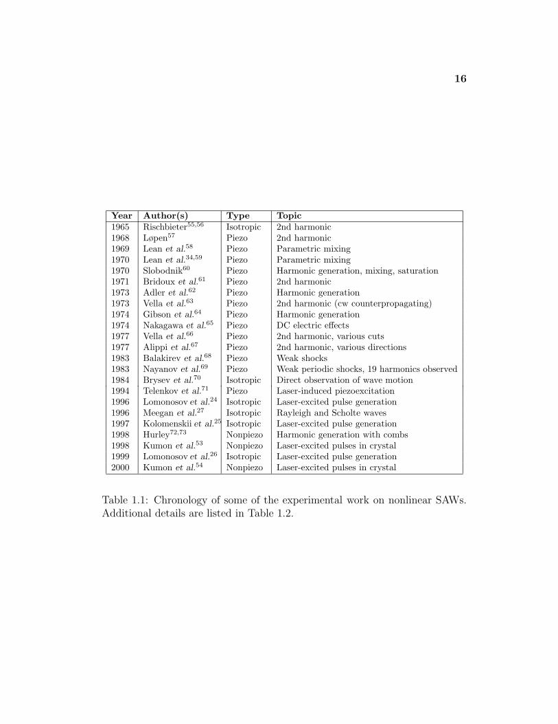
1.1 Chronology of some of the experimental work on nonlinear SAWs.Additional details are listed in Table 1.2. . . . . . . . . . . . . . 16
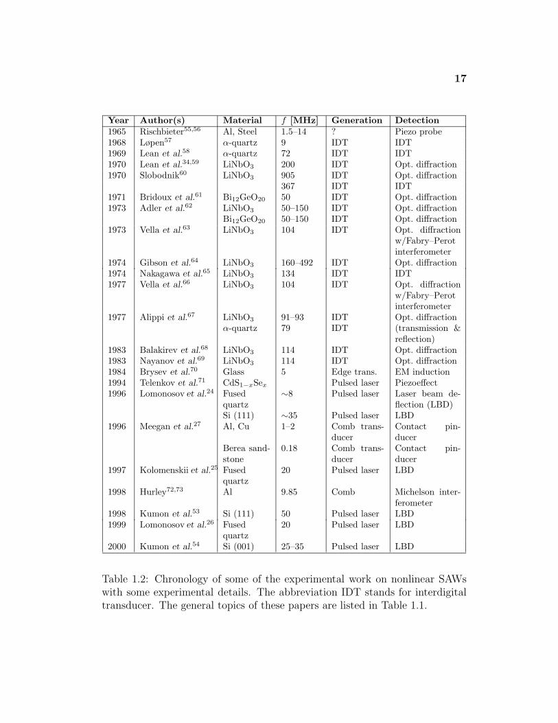
1.2 Chronology of some of the experimental work on nonlinear SAWswith some experimental details. The general topics of these pa-pers are listed in Table 1.1. . . . . . . . . . . . . . . . . . . . . . 17
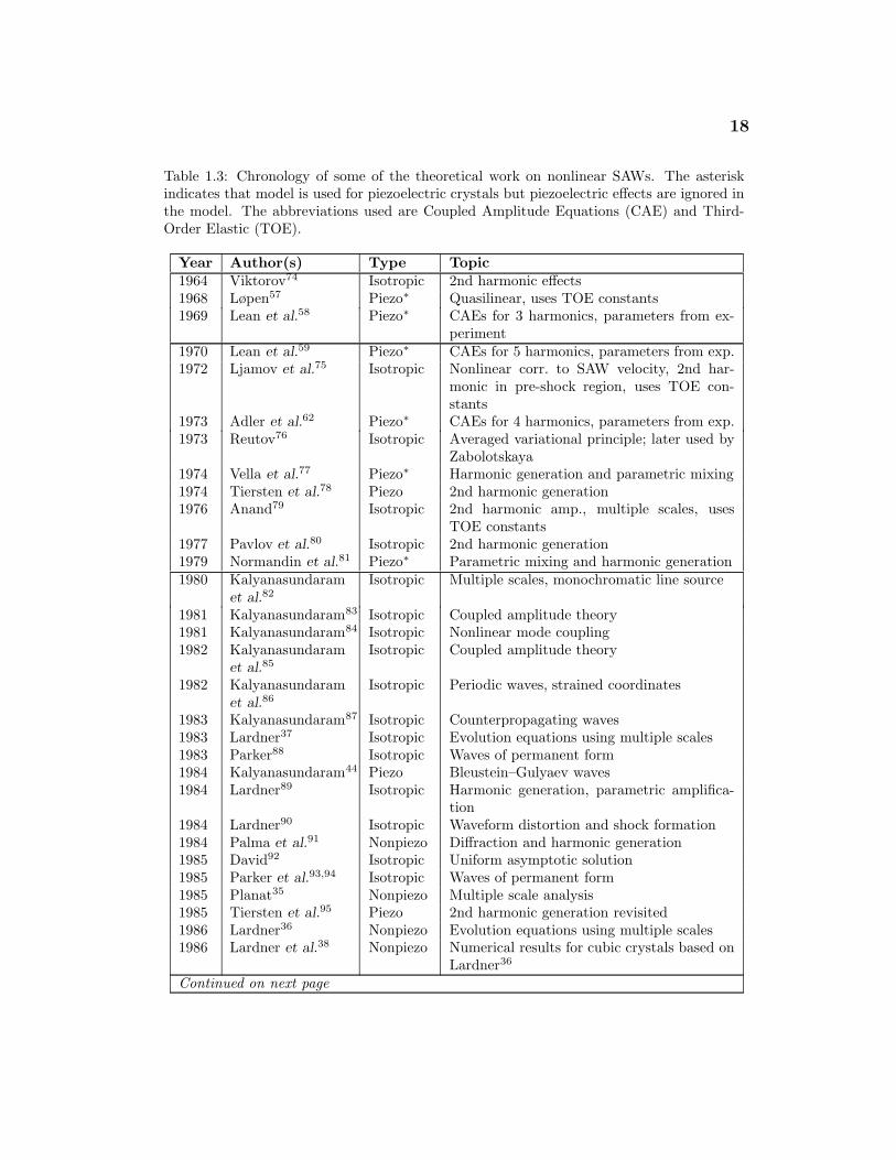
1.3 Chronology of some of the theoretical work on nonlinear SAWs. 18
2.1 Comparison of various approximate solutions of the spectral evo-lution equations for the fundamental and second harmonic nearthe source. . . . . . . . . . . . . . . . . . . . . . . . . . . . . . . 48
2.2 Conversions and analogies between expressions for the linear so-lutions in the isotropic and anisotropic surface acoustic wavetheories. . . . . . . . . . . . . . . . . . . . . . . . . . . . . . . . 54
2.3 Analogies between expressions for nonlinear acoustical parame-ters in the isotropic and anisotropic surface acoustic wave theories. 59
3.1 Point groups of cubic crystals. . . . . . . . . . . . . . . . . . . . 68
3.2 Lattice types, symmetries, and densities of selected nonpiezoe-lectric cubic crystals. . . . . . . . . . . . . . . . . . . . . . . . . 73
3.3 Second-order elastic (SOE) constants for selected nonpiezoelec-tric cubic crystals in the m3m point group. . . . . . . . . . . . . 74
3.4 Third-order elastic (TOE) constants for selected nonpiezoelectriccrystals in the m3m point group. . . . . . . . . . . . . . . . . . 76
3.5 Second-order elastic (SOE) and third-order elastic (TOE) con-stants for selected nonpiezoelectric crystals in the m3 point group. 78
4.1 Listing of selected nonpiezoelectric cubic crystals with exper-imentally determined third-order elastic constants ordered byanisotropy ratio. . . . . . . . . . . . . . . . . . . . . . . . . . . . 81
6.1 Phases of key linear and nonlinear parameters for the selectedpropagation directions in the (111) plane of Si. . . . . . . . . . . 173
6.2 Phases of key linear and nonlinear parameters for the selectedpropagation directions in the (111) plane of KCl. . . . . . . . . 178
xiii
6.3 Phases of key linear and nonlinear parameters for the selectedpropagation directions in the (111) plane of Ni. . . . . . . . . . 185
7.1 Physical, experimental, and numerical parameters for SAW pulsesin the directions 0◦ and 26◦ from 〈100〉 in the (001) plane of crys-talline silicon. . . . . . . . . . . . . . . . . . . . . . . . . . . . . 200
7.2 Physical, experimental, and numerical parameters for SAW pulsesin the directions 0◦ from 〈112〉 in the (111) plane of crystallinesilicon. . . . . . . . . . . . . . . . . . . . . . . . . . . . . . . . . 208
B.1 Summary of some of the theoretical and experimental researchon linear elastic wave propagation in nonpiezoelectric anisotropicmedia of various symmetries. . . . . . . . . . . . . . . . . . . . . 231
B.2 Summary of some of the early theoretical and experimental re-search on linear elastic wave propagation in piezoelectric aniso-tropic media of various symmetries. . . . . . . . . . . . . . . . . 243
B.3 Summary of the various types of surface acoustic waves reviewedin the surface acoustic wave tutorial. . . . . . . . . . . . . . . . 252
xiv
List of Figures
1.1 Horizontal waveforms for nonlinear Rayleigh, Stoneley, and Scholtewaves. . . . . . . . . . . . . . . . . . . . . . . . . . . . . . . . . 7
1.2 Vertical waveforms for nonlinear Rayleigh, Stoneley, and Scholtewaves. . . . . . . . . . . . . . . . . . . . . . . . . . . . . . . . . 8
2.1 Coordinate system for plane wave propagation. . . . . . . . . . 23
2.2 Displacement depth profile for silicon in (001) plane in 〈100〉direction for initially sinusoidal wave. . . . . . . . . . . . . . . . 26
2.3 Schematic representation of a generalized Rayleigh wave in apure mode direction. . . . . . . . . . . . . . . . . . . . . . . . . 26
2.4 Typical particle motion for a generalized Rayleigh wave. . . . . 27
2.5 Plots of the parameters ξ, ξt, ξl, η, ζ , and Λ3 for isotropic mate-rials as a function of Poisson’s ratio σ. . . . . . . . . . . . . . . 57
4.1 Dependence of SAW speed on direction of propagation in the(001) plane for selected materials. . . . . . . . . . . . . . . . . . 84
4.2 Dependence of nonlinearity matrix elements on direction of prop-agation in the (001) plane in selected materials (RbCl, KCl,NaCl, CaF2, SrF2, BaF2, Cs-alum, NH4-alum, K-alum, C, Si,Ge, Al, Ni, Cu). . . . . . . . . . . . . . . . . . . . . . . . . . . . 87
4.3 Dependence of nonlinearity parameters on direction of propaga-tion in the (001) plane of Si. . . . . . . . . . . . . . . . . . . . . 90
4.4 Magnitudes of the SAW components in the (001) plane of Si. . . 94
4.5 Velocity waveforms in selected directions of propagation in the(001) plane of Si. . . . . . . . . . . . . . . . . . . . . . . . . . . 98
4.6 Displacement waveforms in selected directions of propagation inthe (001) plane of Si. . . . . . . . . . . . . . . . . . . . . . . . . 102
4.7 Particle trajectories in selected directions of propagation in the(001) plane of Si. . . . . . . . . . . . . . . . . . . . . . . . . . . 103
4.8 Frequency spectra and harmonic propagation curves for selecteddirections of propagation in the (001) plane of Si. . . . . . . . . 105
4.9 Comparison of selected nonlinearity matrix elements calculatedfrom third-order elastic constant data of (1) McSkimin and An-dreatch and (2) Drabble and Gluyas for propagation in the (001)plane of Si. . . . . . . . . . . . . . . . . . . . . . . . . . . . . . 106
xv
4.10 Dependence of nonlinearity parameters on direction of propaga-tion in the (001) plane of KCl. . . . . . . . . . . . . . . . . . . . 108
4.11 Velocity waveforms in selected directions of propagation in the(001) plane of KCl. . . . . . . . . . . . . . . . . . . . . . . . . . 110
4.12 Frequency spectra and harmonic propagation curves for selecteddirections of propagation in the (001) plane of KCl. . . . . . . . 111
4.13 Comparison of selected nonlinearity matrix elements calculatedfrom third-order elastic constant data of (1) Drabble and Stra-then and (2) Chang for propagation in the (001) plane of KCl. . 115
4.14 Dependence of nonlinearity parameters on direction of propaga-tion in the (001) plane of Ni. . . . . . . . . . . . . . . . . . . . . 117
4.15 Velocity waveforms in selected directions of propagation in the(001) plane of Ni. . . . . . . . . . . . . . . . . . . . . . . . . . . 118
4.16 Frequency spectra and harmonic propagation curves for selecteddirections of propagation in the (001) plane of Ni. . . . . . . . . 119
4.17 Comparison of selected nonlinearity matrix elements calculatedfrom third-order elastic constant data of (1) Salama and Alersand (2) Sarma and Reddy for propagation in the (001) plane ofNi. . . . . . . . . . . . . . . . . . . . . . . . . . . . . . . . . . . 122
5.1 Dependence of SAW speed on direction of propagation in the(110) plane for selected materials. . . . . . . . . . . . . . . . . . 125
5.2 Dependence of nonlinearity matrix elements on direction of prop-agation in the (110) plane in selected materials (RbCl, KCl,NaCl, CaF2, SrF2, BaF2, C, Si, Ge, Al, Ni, Cu). . . . . . . . . . 127
5.3 Dependence of nonlinearity matrix elements on direction of prop-agation in the (110) plane in selected alums (Cs-alum, NH4-alum, K-alum). . . . . . . . . . . . . . . . . . . . . . . . . . . . 129
5.4 Dependence of nonlinearity parameters on direction of propaga-tion in the (110) plane of Si. . . . . . . . . . . . . . . . . . . . . 131
5.5 Velocity waveforms in selected directions of propagation in the(110) plane of Si. . . . . . . . . . . . . . . . . . . . . . . . . . . 132
5.6 Displacement waveforms in selected directions of propagation inthe (110) plane of Si. . . . . . . . . . . . . . . . . . . . . . . . . 133
5.7 Particle trajectories in selected directions of propagation in the(110) plane of Si. . . . . . . . . . . . . . . . . . . . . . . . . . . 134
5.8 Frequency spectra and harmonic propagation curves for selecteddirections of propagation in the (110) plane of Si. . . . . . . . . 135
5.9 Dependence of nonlinearity parameters on direction of propaga-tion in the (110) plane of KCl. . . . . . . . . . . . . . . . . . . . 138
xvi
5.10 Velocity waveforms in selected directions of propagation in the(110) plane of KCl. . . . . . . . . . . . . . . . . . . . . . . . . . 139
5.11 Frequency spectra and harmonic propagation curves in selecteddirections of propagation in the (110) plane of KCl. . . . . . . . 140
5.12 Dependence of nonlinearity parameters on direction of propaga-tion in the (110) plane of Ni. . . . . . . . . . . . . . . . . . . . . 143
5.13 Velocity waveforms in selected directions of propagation in the(110) plane of Ni. . . . . . . . . . . . . . . . . . . . . . . . . . . 144
5.14 Frequency spectra and harmonic propagation curves for selecteddirections of propagation in the (110) plane of Ni. . . . . . . . . 145
6.1 Dependence of SAW speed on direction of propagation in the(111) plane for selected materials. . . . . . . . . . . . . . . . . . 149
6.2 Dependence of nonlinearity matrix elements on direction of prop-agation in the (111) plane in selected materials (RbCl, KCl,NaCl, CaF2, SrF2, BaF2). . . . . . . . . . . . . . . . . . . . . . 152
6.3 Dependence of nonlinearity matrix elements on direction of prop-agation in the (111) plane in selected materials (C, Si, Ge, Al,Ni, Cu). . . . . . . . . . . . . . . . . . . . . . . . . . . . . . . . 153
6.4 Dependence of nonlinearity matrix elements on direction of prop-agation in the (111) plane in selected alums (Cs-alum, NH4-alum, K-alum). . . . . . . . . . . . . . . . . . . . . . . . . . . . 154
6.5 Transformation of waveforms for various phase angles 0 ≤ θ ≤180◦ of the transformed nonlinearity matrix elements Sθ
lm =
Slmei(n/|n|)θ, where n = l + m. . . . . . . . . . . . . . . . . . . . 160
6.6 Transformation of waveforms for various phase angles −180◦ ≥θ ≥ 0 of the transformed nonlinearity matrix elements Sθ
lm =
Slmei(n/|n|)θ. . . . . . . . . . . . . . . . . . . . . . . . . . . . . . 161
6.7 Comparison of simulated nonlinear waveform distortion betweenvθ
1(x, τ)-transformed nonlinear Rayleigh waves in steel and non-linear SAWs in the direction 0◦ from 〈112〉 in the (111) plane ofSi, Ni, and KCl. . . . . . . . . . . . . . . . . . . . . . . . . . . . 163
6.8 Comparison of simulated nonlinear waveform distortion betweenvθ
1(x, τ)-transformed nonlinear Rayleigh waves in steel and non-linear SAWs in the directions 10◦, 20◦, and 28◦ from 〈112〉 in the(111) plane of KCl. . . . . . . . . . . . . . . . . . . . . . . . . . 165
6.9 Dependence of nonlinearity parameters on direction of propaga-tion in the (111) plane of Si. . . . . . . . . . . . . . . . . . . . . 167
6.10 Velocity waveforms in selected directions of propagation in the(111) plane of Si. . . . . . . . . . . . . . . . . . . . . . . . . . . 169
xvii
6.11 Displacement waveforms in selected directions of propagation inthe (111) plane of Si. . . . . . . . . . . . . . . . . . . . . . . . . 170
6.12 Particle trajectories in selected directions of propagation in the(111) plane of Si. . . . . . . . . . . . . . . . . . . . . . . . . . . 171
6.13 Frequency spectra and harmonic propagation curves for selecteddirections of propagation in the (111) plane of Si. . . . . . . . . 172
6.14 Dependence of nonlinearity parameters on direction of propaga-tion in the (111) plane of KCl. . . . . . . . . . . . . . . . . . . . 177
6.15 Velocity waveforms in selected directions of propagation in the(111) plane of KCl. . . . . . . . . . . . . . . . . . . . . . . . . . 179
6.16 Frequency spectra and harmonic propagation curves for selecteddirections of propagation in the (111) plane of KCl. . . . . . . . 180
6.17 Dependence of nonlinearity parameters on direction of propaga-tion in the (111) plane of Ni. . . . . . . . . . . . . . . . . . . . . 184
6.18 Velocity waveforms in selected directions of propagation in the(111) plane of Ni. . . . . . . . . . . . . . . . . . . . . . . . . . . 186
6.19 Frequency spectra and harmonic propagation curves for selecteddirections of propagation in the (111) plane of Ni. . . . . . . . . 187
7.1 Schematic diagram of the experimental apparatus for photoe-lastic nonlinear surface acoustic wave generation with dual laserprobe detection. . . . . . . . . . . . . . . . . . . . . . . . . . . . 193
7.2 Nonlinearity matrix elements S11, S12, S13 for crystalline siliconin the (001) plane as a function of direction. Due to the symme-tries of this cut, the matrix elements are symmetric about 45◦and periodic every 90◦. . . . . . . . . . . . . . . . . . . . . . . . 199
7.3 Comparison of experiment and theory for a surface acoustic wavepulse propagating in the direction 0◦ from 〈100〉 in the (001)plane of crystalline silicon. . . . . . . . . . . . . . . . . . . . . . 202
7.4 Comparison of experiment and theory for a surface acoustic wavepulse propagating in the direction 26◦ from 〈100〉 in the (001)plane of crystalline silicon. . . . . . . . . . . . . . . . . . . . . . 204
7.5 Comparison of experiment and theory for surface acoustics wavespropagating in the 〈112〉 direction in the (111) plane of crys-talline silicon. . . . . . . . . . . . . . . . . . . . . . . . . . . . . 207
7.6 Comparison of experimental and theoretical longitudinal veloc-ity waveforms reconstructed with shading functions of approxi-mately 700 MHz bandwidth and exactly 3000 MHz bandwidth.The waveforms are the result of propagation in the direction 0◦from 〈112〉 in the (111) plane of crystalline silicon. . . . . . . . . 211
B.1 Schematic representations of a Rayleigh wave and Stoneley wave. 223
xviii
B.2 Schematic representations of a Scholte wave and Leaky Rayleighwave. . . . . . . . . . . . . . . . . . . . . . . . . . . . . . . . . . 223
B.3 Typical particle motion for a generalized Rayleigh wave. . . . . 226
B.4 Displacement depth profile for silicon in (001) plane in 〈100〉direction for initially sinusoidal wave. . . . . . . . . . . . . . . . 227
B.5 Schematic representation of a generalized Rayleigh wave in apure mode direction. . . . . . . . . . . . . . . . . . . . . . . . . 227
B.6 Examples of polar plots of relative speed and slowness (based onsilicon in (001) plane). . . . . . . . . . . . . . . . . . . . . . . . 228
B.7 Effect of power flow vector P not being parallel to propagationvector k. . . . . . . . . . . . . . . . . . . . . . . . . . . . . . . . 228
B.8 Schematic diagram of an exceptional bulk wave (surface skim-ming bulk wave) in side and front perspectives. . . . . . . . . . 234
B.9 Coupling between pseudo-surface wave mode and bulk modepropagating at angle θ to the surface. . . . . . . . . . . . . . . . 236
B.10 Schematic representation of a Bleustein–Gulyaev wave. . . . . . 244
D.1 Typical planes for crystal cuts in cubic crystals as specified usingMiller index notation. . . . . . . . . . . . . . . . . . . . . . . . . 273
xix
List of Symbols
A amplitude factor (anisotropic media)A′ linear combination of absorption coefficientsA′′ another linear combination of absorption coefficientsAn dimensionless absorption coefficient (n integer)
Bj =∑3
s=1 β(s)j waveform amplitude at surface (j ∈ {1, 2, 3})
BRj waveform amplitude at surface for Rayleigh wave (j ∈
{1, 2, 3})C constant prefactor of time-domain evolution equation
(isotropic media)Cs coefficients in linear solution (s ∈ {1, 2, 3})CS constant prefactor of time-domain evolution equation
(anisotropic media)D dimensionless diffraction parameterE elastic potential energy densityE2 elastic potential energy density terms of quadratic orderE3 elastic potential energy density terms of cubic orderFs1s2s3 parameters in expansion for Slm (s1, s2, s3 ∈ {1, 2, 3})H Hamiltonian functionH Hilbert transformI amplitude factor (isotropic media)L kernel of integral in time-domain evolution equation
(isotropic media)LS kernel of integral operator in time-domain evolution
equation (anisotropic media)M Mach number or peak strainN number of harmonicsPlm factor in kernel LS (l, m integers)Qlm factor in kernel LS (l, m integers)Rlm nonlinearity matrix (isotropic media; l, m integers)Slm nonlinearity matrix (l, m integers)SR
lm nonlinearity matrix of Rayleigh wave (l, m integers)
Slm = −Slm/c44 dimensionless nonlinearity matrix (l, m integers)T kinetic energy per unit area
xx
T period of waveformT1 taper function for quasilinear solutionV potential energy per unit area terms of quadratic orderVn dimensionless velocity spectral component (n integer)
Vn dimensionless velocity spectral component with taperfunction (n integer)
W kinetic energy per unit area terms of cubic orderW component term of WX dimensionless length variable∆X dimensionless step size in numerical integration∆Xinit dimensionless initial step sizeXswitch range for ∆Xinit
Xmax maximum range for numerical integrationan spectral component functions and generalized coordi-
nates (n integer)bn slowly varying amplitude functions (n integer)c phase speedcR phase speed of Rayleigh waves (isotropic media)cl phase speed of longitudinal bulk wavesct phase speed of transverse bulk wavescijkl second-order elastic (SOE) constants (i, j, k, l ∈ {1, 2, 3})d diameter of beamdijklmn third-order elastic (TOE) constants (i, j, k, l, m, n ∈
{1, 2, 3})eij strain tensor (i, j ∈ {1, 2, 3})f0 characteristic frequencyffund fundamental frequencyi imaginary unit (when not as an index)k wave numberki wave vector components (i ∈ {1, 2, 3})li and l
(s)i penetration depth parameter components (i, s ∈
{1, 2, 3})pn generalized momenta (n integer)t timeui particle displacement components (i ∈ {1, 2, 3})uni depth eigenfunctions (i ∈ {1, 2, 3}, n integer)v0 characteristic velocityvi velocity component in xi-direction (i ∈ {1, 2, 3})
xxi
vl characteristic velocity for lossless bulk wavevn velocity spectral component (n integer)vR
n velocity spectral component for Rayleigh wave (n integer)vx longitudinal velocity componentvx0 amplitude of longitudinal velocity time waveformvy transverse velocity componentvz vertical velocity componentvz0 characteristic measured vertical velocity componentwn1n2n3 coefficients in expansion for Wxi position coordinates (i ∈ 1, 2, 3)x0 characteristic lengthx11 shock formation distance for nonlinear surface wave (as
function of spectral component v0 and nonlinearity ma-trix element S11); equal to xx0
11
xl shock formation distance for bulk waves in a fluidxx0
11 shock formation distance for nonlinear surface wave (asfunction of longitudinal velocity vx0 and nonlinearity ma-trix element S11); equal to x11
xmax probe beam separationx ≡ x1 longitudinal position coordinatey ≡ x2 transverse position coordinatez ≡ x3 vertical position coordinatez0 Rayleigh distance of beamΓ Gol’dberg numberΓik = cijklljll matrix associated with linearized wave equation (i, k ∈
{1, 2, 3})Λ conversion factor between Rlm and Slm
Φ electric potential
αi and α(s)i particle displacement amplitude components (i, s ∈
{1, 2, 3})αn absorption coefficient for n harmonic (n integer)β coefficient of nonlinearity for surface wave (relative to
spectral component v0)βl coefficient of nonlinearity for lossless bulk waveβx0 coefficient of nonlinearity for surface wave (relative to
longitudinal velocity vx0)
β(s)j = Csα
(s)j coefficient in nonlinear solution (j, s ∈ {1, 2, 3})
δij Kronecker delta function (i, j ∈ {1, 2, 3})
xxii
ε acoustic Mach number for surface wave (relative to thelongitudinal velocity vx0)
εl acoustic Mach number for bulk wave in fluidεx0 acoustic Mach number for surface wave (relative to the
longitudinal velocity vx0)ζ numerical factor (isotropic media)
ζs ≡ l(s)3 penetration depth parameters (s ∈ 1, 2, 3)
η numerical parameter (isotropic media)θ phase angleθlong transforming phase for longitudinal velocity componentθtran transforming phase for transverse velocity componentθvert transforming phase for vertical velocity componentλ wavelengthµ bulk shear modulusξ ratio of Rayleigh and shear wave speeds (isotropic media)ξl penetration depth parameter (isotropic media)ξt penetration depth parameter (isotropic media)ρ mass densityσ Poisson’s ratioσij stress tensor (i, j ∈ {1, 2, 3})φBj phase of Bj (j ∈ {1, 2, 3})φvj phase of vj (j ∈ {1, 2, 3})φ
(s)j phase of β
(s)j (j, s ∈ {1, 2, 3})
ω and ω0 angular frequency
xxiii
Chapter 1
Introduction
Surface acoustic waves (SAWs) are waves that exist at an interface between
a solid and a vacuum, gas, liquid, or another solid. They typically have most
of their energy contained close (within approximately one wavelength) to the
interface region. In contrast, the more widely studied bulk acoustic waves,
which do not require an interface in order to travel in a solid, typically have
their energy distributed more broadly throughout the medium in which they
travel.
SAWs were first formally identified and described by Lord Rayleigh1 in
1885. Due to the difficulty of solving the equations to describe these waves even
for simple cases, little additional work was done until the 1950s and 1960s, when
the computation power of the digital computer became available. Since then,
many different kinds of SAWs have been described, and many applications of
SAWs have been invented. Early theories focused on deriving and solving the
simpler linear equations for small amplitude waves. Eventually experiments
began generating the finite amplitude SAWs which are of sufficiently high in-
tensity that more complicated, nonlinear equations are needed to explain the
resulting waves.
SAWs have several properties that distinguish them from bulk waves.
First, SAWs exhibit only two-dimensional geometrical spreading, i.e., the en-
ergy of the SAW spreads out primarily in the two-dimensional interface region
instead of spreading throughout the whole three-dimensional medium like a
1
2
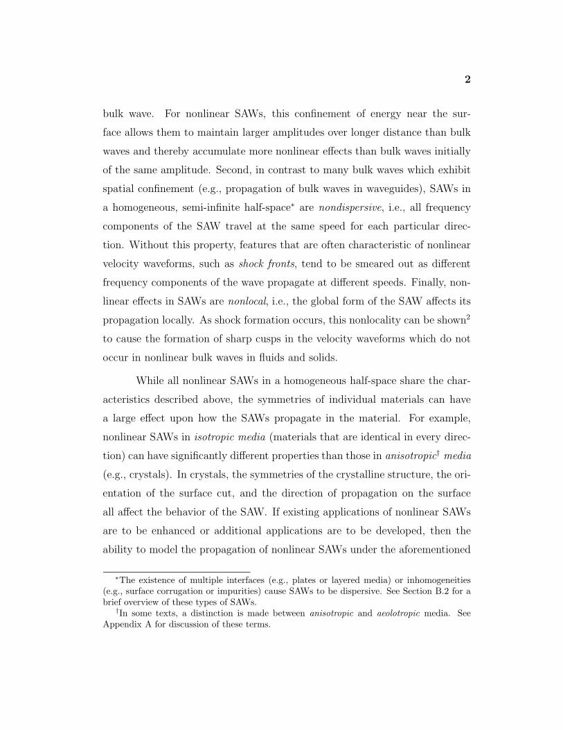
bulk wave. For nonlinear SAWs, this confinement of energy near the sur-
face allows them to maintain larger amplitudes over longer distance than bulk
waves and thereby accumulate more nonlinear effects than bulk waves initially
of the same amplitude. Second, in contrast to many bulk waves which exhibit
spatial confinement (e.g., propagation of bulk waves in waveguides), SAWs in
a homogeneous, semi-infinite half-space∗ are nondispersive, i.e., all frequency
components of the SAW travel at the same speed for each particular direc-
tion. Without this property, features that are often characteristic of nonlinear
velocity waveforms, such as shock fronts, tend to be smeared out as different
frequency components of the wave propagate at different speeds. Finally, non-
linear effects in SAWs are nonlocal, i.e., the global form of the SAW affects its
propagation locally. As shock formation occurs, this nonlocality can be shown2
to cause the formation of sharp cusps in the velocity waveforms which do not
occur in nonlinear bulk waves in fluids and solids.
While all nonlinear SAWs in a homogeneous half-space share the char-
acteristics described above, the symmetries of individual materials can have
a large effect upon how the SAWs propagate in the material. For example,
nonlinear SAWs in isotropic media (materials that are identical in every direc-
tion) can have significantly different properties than those in anisotropic† media
(e.g., crystals). In crystals, the symmetries of the crystalline structure, the ori-
entation of the surface cut, and the direction of propagation on the surface
all affect the behavior of the SAW. If existing applications of nonlinear SAWs
are to be enhanced or additional applications are to be developed, then the
ability to model the propagation of nonlinear SAWs under the aforementioned
∗The existence of multiple interfaces (e.g., plates or layered media) or inhomogeneities(e.g., surface corrugation or impurities) cause SAWs to be dispersive. See Section B.2 for abrief overview of these types of SAWs.
†In some texts, a distinction is made between anisotropic and aeolotropic media. SeeAppendix A for discussion of these terms.
3
conditions must obtained. While much work has been done to understand
nonlinear SAWs in isotropic media and several theories have been advanced
for anisotropic media, few detailed calculations have been performed describ-
ing the propagation of nonlinear SAWs in actual crystals. Performing these
calculations and interpreting the results are the focuses of the present work.
However, because of the wide variety of anisotropic media, the scope of
the dissertation is limited to nonpiezoelectric, cubic crystals. Only materials
with cubic symmetry are considered, not because this is a limitation of the
theoretical model, but because they have the highest symmetry of all crystal
types and are simplest in that sense. In addition, cubic crystals have been
widely studied experimentally, and many data are available on their mechan-
ical properties. Only nonpiezoelectric materials are considered because the
coupling between the mechanical and electrical forces which occurs in piezo-
electric crystals introduces significantly more complexity to the problem. Even
with the above restrictions, many materials fall into this subset of anisotropic
media, including a variety of common dielectrics, semiconductors, metals, and
metallic alloys.
The remainder of this chapter (1) briefly defines and reviews the various
types of SAWs to provide a context for subsequent discussions; (2) briefly
discusses the various applications that have been implemented or proposed for
linear and nonlinear SAWs; and (3) reviews the literature of theoretical and
experimental work on the nonlinear SAWs in crystals.
1.1 Types and Properties
Excellent reviews of the types and properties of SAWs have been given by
Farnell,3,4 Farnell and Adler,5 Stegeman and Nizzoli,6 Feldmann and Henaff,7
and Biryukov et al.8 in the linear regime, and by Parker9 and Mayer10 in the
4
nonlinear regime. Only a brief review of the various cases is given here. A
lengthier tutorial on the types of SAWs is provided in Appendix B.
Depending on the type of interface, SAWs in a homogeneous, isotropic
half-space are classified as Rayleigh waves (solid–vacuum), Stoneley waves
(solid–solid), or Scholte waves (solid–fluid).∗ In these cases, the particle dis-
placement is contained within the sagittal plane, and the amplitude of the
displacement decays exponentially away from the interface into the solid. Due
to the isotropy, the SAW speed is constant in all directions and strictly less
than all the bulk wave speeds in the material.
Several distinguishing linear effects appear in anisotropic media. Par-
ticle displacement is generally no longer confined to the sagittal plane, and it
decays away into the solid as an exponentially damped sinusoid. Such waves
are called generalized Rayleigh waves. In addition, other effects are possible, in-
cluding deeply penetrating surface waves called quasi-bulk surface waves, bulk
waves that satisfy the traction-free surface boundary condition called excep-
tional or “surface-skimming” bulk waves, and unstable surface waves that ra-
diate into the solid, called pseudo-surface waves. In addition, the SAW speed
is a function of both the orientation of the crystal with respect to the surface
cut and the direction of propagation, and the acoustic power flow of the SAW
is no longer necessarily coincident with the direction of the wave vector.
Thus, even in the linear regime, many additional phenomena appear in
anisotropic materials as compared to isotropic media. As shown below, this
trend continues in the nonlinear regime. While nonlinear SAWs in anisotropic
media have some features qualitatively similar to those in isotropic media, their
∗Cases where the sound radiates from the solid into the liquid are usually called leakyRayleigh waves. In these cases the amplitude of the displacement grows exponentially intothe fluid.
5
overall behavior is often distinctly different. These similarities and differences
are discussed at length in the following chapters.
1.2 Applications
A large number of applications for SAWs have been devised, and this section
reviews only some of the developments. SAW devices have been designed to
perform signal processing. Filters, oscillators, and pulse compressors and ex-
panders have been developed using linear effects, while convolvers, correlators,
amplifiers, and memory elements have been developed using nonlinear effects.11
Many of these components are used in mobile and wireless communication de-
vices for personal communication services (e.g., pagers, cellular phones), wide
area networks, and wireless local area networks.12 SAWs have also been used to
perform nondestructive evaluation (NDE). Defects, material properties (den-
sity, elastic constants), applied and residual stresses, adhesive bonding, surface
roughness, plate and layer thickness may all been measured using linear SAWs,
and the use of nonlinear SAWs to test materials is a subject of current research.
SAW sensors have been designed to detect the presence of chemical species and
measure changes in temperature, pressure, and voltage. For a reviews of these
topics, the reader is referred to Oliner,13 Feldmann and Henaff,7 and Biryukov
et al8 (SAW devices), Viktorov,14 Curtis,15 Krautkramer and Krautkramer16
(NDE), and Thompson and Stone17 (SAW sensors). In addition, Appendix C
contains a more detailed tutorial about these applications and many more.
6
1.3 Literature Review
1.3.1 Nonlinear Rayleigh, Stoneley, and Scholte Waves
The nonlinear behavior of Rayleigh waves has been described at length by many
authors, and therefore only a brief review of the most recent work is given here.
Shull et al.18 and Knight et al.19 provide literature reviews of the various the-
oretical and experimental works, as well as a plethora of numerical results for
a variety of cases. Using the theory of Zabolotskaya,20 Shull et al. examined
the behavior of plane,18 cylindrical,18 and diffracting21 nonlinear waves, while
Knight et al. provided a rigorous generalization of the theory19 to nonplanar
waves and pulses, derived approximate expressions for the shock formation
distance,22 and described the propagation of transient waveforms.23 Experi-
mentally, very high amplitude SAWs have been generated photoelastically in
fused quartz and crystalline silicon via pulsed laser excitation.24,25 Calculations
by Knight et al.19,22 were verified by comparison with measurements26 of SAW
pulses in fused quartz.
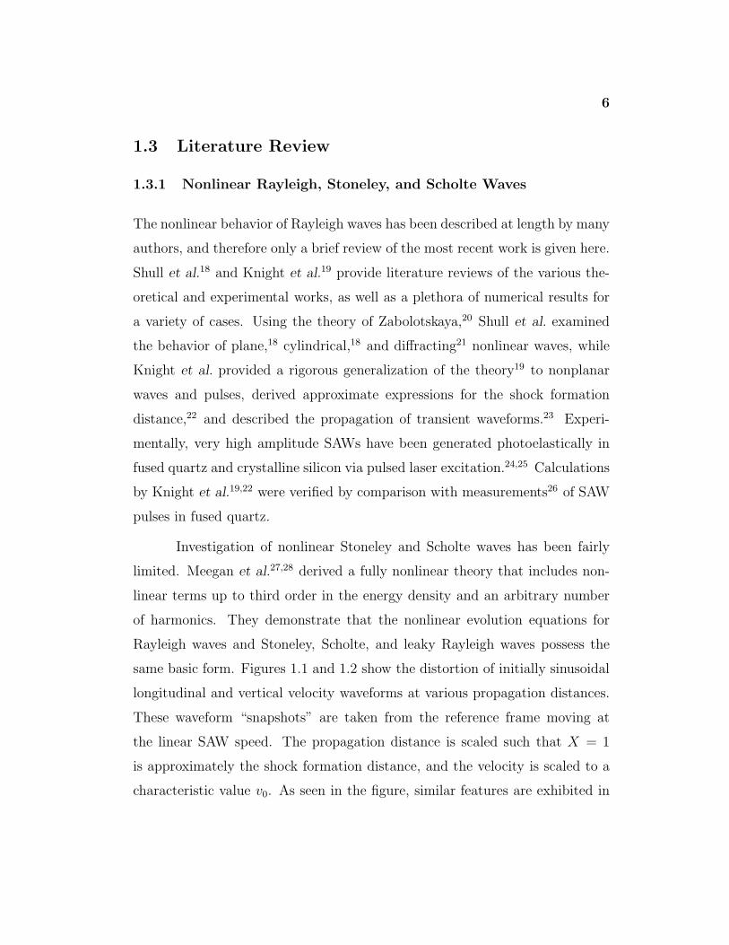
Investigation of nonlinear Stoneley and Scholte waves has been fairly
limited. Meegan et al.27,28 derived a fully nonlinear theory that includes non-
linear terms up to third order in the energy density and an arbitrary number
of harmonics. They demonstrate that the nonlinear evolution equations for
Rayleigh waves and Stoneley, Scholte, and leaky Rayleigh waves possess the
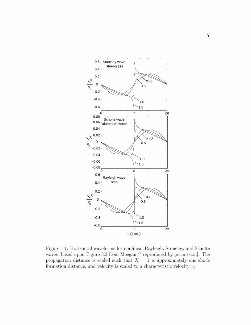
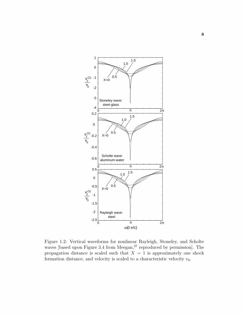
same basic form. Figures 1.1 and 1.2 show the distortion of initially sinusoidal
longitudinal and vertical velocity waveforms at various propagation distances.
These waveform “snapshots” are taken from the reference frame moving at
the linear SAW speed. The propagation distance is scaled such that X = 1
is approximately the shock formation distance, and the velocity is scaled to a
characteristic value v0. As seen in the figure, similar features are exhibited in
7
-0.6
-0.4
-0.2
0
0.2
0.4
Rayleigh wave:steel
0 π 2π
-0.6
-0.4
-0.2
0
0.2
0.4
0.6steel-glass
-0.08
-0.06
-0.04
-0.02
0
0.02
0.04
0.06
0.08
aluminum-water
0 π 2π
0 π 2π
0.6
ω(t-x/c)
vx
0
vx(1)
v0
vx(1)
v0
1.5
1.0
X=00.5
1.5
1.0
X=0
1.5
1.0
X0.5
Scholte wave:
0.5
(1)
v
Stoneley wave:
=0
Figure 1.1: Horizontal waveforms for nonlinear Rayleigh, Stoneley, and Scholtewaves [based upon Figure 3.3 from Meegan,27 reproduced by permission]. Thepropagation distance is scaled such that X = 1 is approximately one shockformation distance, and velocity is scaled to a characteristic velocity v0.
8
-4
-3
-2
-1
0
1
-2.5
-2
-1.5
-1
-0.5
0
0.5
Rayleigh wave:steel
Stoneley wave:steel-glass
0 π 2π
0 π 2π
0 π 2π
-0.6
-0.4
-0.2
0
0.2
Scholte wave:aluminum-water
ω(t-x/c)
vz(1)
v0
vz(1)
v0
vz(1)
v0
1.51.0
X=00.5
1.51.0
X=00.5
1.51.0
X=00.5
Figure 1.2: Vertical waveforms for nonlinear Rayleigh, Stoneley, and Scholtewaves [based upon Figure 3.4 from Meegan,27 reproduced by permission]. Thepropagation distance is scaled such that X = 1 is approximately one shockformation distance, and velocity is scaled to a characteristic velocity v0.
9
each nonlinear waveform. See Section B.1.1 for additional discussion of some
of the features of these waveforms.
A series of theories by Gusev et al. on the propagation of nonlinear
Rayleigh waves29 and Scholte waves30 (also SAWs in anisotropic media31) has
also been proposed. Their evolution equations differ from those derived using
the dynamical approach of Parker32 and the Hamiltonian approach of Zabolot-
skaya.20 Knight et al.19 proved that the theories of Parker and Zabolotskaya
are equivalent for Rayleigh waves, while Meegan et al.28 have identified incon-
sistencies in the approach of Gusev et al. The interested reader is referred to
their discussions for more details.
1.3.2 Nonlinear Surface Waves in Crystals
Because many practical applications of SAWs require the use of crystals (espe-
cially piezoelectric crystals), extensive work has been done to understand the
propagation of nonlinear SAWs in anisotropic media. For reference purposes,
a tabular summary of much of the experimental and theoretical work is pro-
vided at the end of this chapter. Table 1.1 describes some of the experimental
work that has been done to study nonlinear SAWs. Each entry in Table 1.1
corresponds to an entry in Table 1.2, which lists some of the experimental
parameters and techniques for that work. Table 1.3 summarizes some of the
theoretical work on nonlinear SAWs. None of the tables is exhaustive. In addi-
tion, the tables do not list work that involves dispersion (layer or plate waves),
wedge waves, noncollinear SAW beams, or the interaction of SAWs with bulk
waves.
The most extensive reviews of work on nonlinear SAWs have been given
by Parker9 and Mayer.10 As noted above, Shull et al.18 and Knight et al.19 have
written compact literature reviews that focus primarily on nonlinear Rayleigh
10
waves. However, because these reviews covered much of the experimental work
on nonlinear SAWs, they also cover much of the work that had been done
for crystals. More recently, Hamilton et al.33 reviewed the work on nonlinear
SAWs in nonpiezoelectric crystals. The presentation below includes a summary
of theoretical work on nonlinear SAWs in nonpiezoelectric and piezoelectric
crystals and recent experimental work on nonlinear SAWs in crystals.
Theoretical Work on Nonpiezoelectric Crystals
In the mid-1980s, rigorous theories began to be developed to predict the propa-
gation of nonlinear SAWs in nonpiezoelectric crystals (despite the scepticism of
some earlier researchers∗). Planat35 developed a theory for an elastic solid with
general anisotropy based on a multiple scales approach. He gave numerical
results for the evolution of the amplitude and phase of the first five harmonics
in quartz (neglecting piezoelectric effects), although only a total of eight har-
monics were kept in the calculations. Subsequent work on Rayleigh waves18
shows that an insufficient number of harmonics can introduce anomalies into
the numerical results unless only very weak nonlinearity is considered.
Another theory using multiple scales was developed by Lardner36 based
on his work with nonlinear Rayleigh waves.37 The theory was used by Lardner
and Tupholme38 to investigate the properties of cubic crystals for which the
free surface is a plane of symmetry and the direction of propagation is along
one of the crystal axes. Results were given in terms of tables of coefficients
describing the growth and decay rates of the fundamental, second, and third
∗Interestingly, Lean et al.34 wrote in 1970, “Due to the dispersionless property of Rayleighwaves, the harmonic generation of Rayleigh waves unlike the optical second-harmonic gen-eration does not have any limit in the number of harmonics generated. The large numberof harmonics generated plus the complexity of two-dimensional inhomogeneous waves makestheoretical calculation on the surface acoustic wave harmonic generation extremely compli-cated, if not impossible.”
11
harmonics for a wide variety of cubic crystals, as well as the first three harmonic
propagation curves for the specific example of MgO. Lardner and Tupholme
also showed that for Ge the harmonic growth and decay rates are extremely
sensitive to changes in the third-order elastic constants d111, d112, and d155 and
therefore concluded that measurements using harmonic generation may offer
an accurate way to determine third-order elastic constants. Later papers by
Harvey and Tupholme39,40 extended the method to include multiple waves that
travel in the same or opposite directions, also called co-directional waves. They
presented the following results for MgO: (1) harmonic propagation curves for
the fundamental, second, fifth, and sixth harmonics of co-directional waves
traveling in the directions 0◦ and 40◦ from 〈100〉 in the (001) plane,39 and (2)
growth and decay rates for both single and co-directional waves over the range
of directions 0◦ to 45◦ from 〈100〉 in the (001) plane.40
Independently, Parker32 developed a theory for nonpiezoelectric, ani-
sotropic media that avoids some of the complications and limitations of the
multiple scales approach. This was done by introducing a reference frame
moving at the linear wave speed and then deriving evolution equations for the
wave in the frequency domain. Results for this theory were given only in terms
of waveforms for an isotropic solid (however, see the discussion of piezoelectric
crystals below). A class of waveforms was presented that Parker claimed to be
“non-distorting profiles.” However, Hamilton et al.41 later showed that such
profiles only arise if artificial constraints are imposed on the frequency spec-
trum, such as abrupt truncation or gradual amplitude shading of the Fourier
series representation of a periodic waveform. Kalyanasundaram et al.42 later
extended Parker’s theory to include diffraction effects.
During the mid-1990s, Hamilton et al.43 extended the theory of Zabolot-
skaya20 for nonlinear Rayleigh waves to include nonpiezoelectric, anisotropic
12
media. Longitudinal and vertical velocity waveforms were presented for KCl
in the [112] direction in the (111) plane and the [100] direction in the (001)
plane, although the authors made it clear that this is not a limitation of the
approach. A later paper by Hamilton et al.33 also shows the harmonic propaga-
tion curves for the first five harmonics for both of these cases. Like the theory of
Parker,32 the theory of Hamilton et al. also develops evolution equations in the
frequency domain. However, unlike the theory of Parker, the model equations
of Hamilton et al. are derived using a Hamiltonian approach (see Chapter 2
for a description). Hamilton et al.33 have shown that their theory for non-
linear SAWs in anisotropic media reduces to the theory of Zabolotskaya20 for
nonlinear Rayleigh waves in the isotropic limit.
Gusev et al.31 has also developed a theory for nonlinear SAWs in ani-
sotropic media, but did not provide any numerical calculations demonstrating
their results. The evolution equations are given in the time domain and differ
from those given by Parker32 and Hamilton et al.33
Theoretical Work with Piezoelectric Crystals
Several theories have also been developed to model nonlinear SAW propaga-
tion in piezoelectric crystals (see Section B.1.6 for an introductory discussion).
Based on approaches previously used to model Rayleigh waves, Kalyanasun-
daram44 derived a theory for the special case of Bleustein–Gulyaev waves (see
Section B.1.7) under the assumption that only third-order nonlinearity (quar-
tic anharmonicity) affects the propagation. Mayer45 later extended the theory
to include both second-order and third-order nonlinearity. In 1988, Tupholme
and Harvey46 developed the first general theory for nonlinear SAWs in piezo-
electric crystals by using the method of multiple scales employed previously by
Lardner36 and requiring open circuit electrical boundary conditions (see Sec-
13
tion B.1.6 for a description of electrical boundary conditions at the surface).
Numerical results were later presented by Harvey et al.47 in the form of prop-
agation curves for the fundamental, second, and third harmonics for a wave
propagating along the positive X axis in the Y cut of LiNbO3. Simulations
performed with two different data sets showed significant differences. Addi-
tional papers by Harvey and Tupholme39,40 considered co-directional waves.
They presented the following results for LiNbO3: (1) harmonic propagation
curves for the fundamental, second, fifth, and sixth harmonics of co-directional
waves traveling in the directions 0◦ and 40◦ from the X axis in the Y cut,39
and (2) growth and decay rates for both single and co-directional waves over
the range of directions 0◦ to 90◦ from the X axis in the Y cut.40
Around the same time, Parker and David48 developed a theory for non-
linear SAWs in piezoelectric media based on the approach of Parker32 described
above, and presented simulations showing the evolution of waveforms along the
X and Z axes in the Y cut of LiNbO3 for earthed, open circuit, and free space
electrical boundary conditions. In a later paper by David and Parker,49 “non-
distorting waveforms” were presented for propagation along the X and Z axes
in the Y cut of LiNbO3. However, as noted above, Hamilton et al.41 showed
that stationary Rayleigh waves arise only for the artificial condition of a finite
number of harmonics. Since David and Parker used only forty harmonics in
their simulations, this may also be the cause of the non-distorting profiles in
their results. Diffraction effects were added to the model of Parker and David
by Kalyanasundaram et al.42
Hamilton et al.50 have also developed a theory for nonlinear SAWs in
piezoelectric crystals by generalizing their theory for nonpiezoelectric crystals.33
Free space, shorted, and open circuit electrical boundary conditions may be
included. Simulations have been presented51 for monofrequency waveforms
14
propagating in the X and Y axis directions in the Z cut of LiNbO3. Recent
papers by Hamilton et al.51,52 discuss how all three theories for isotropic solids,
nonpiezoelectric crystals, and piezoelectric crystals are constructed under a
single framework.
Experimental Work with Crystals
Until the mid-1990s, much of the experimental work on nonlinear SAWs in
crystals was limited to measurements of the first few harmonics. In 1996,
Lomonosov and Hess24 presented results of pulsed SAWs generated using a
photoelastic technique. In this approach, an infrared laser is focused into a
small strip on the free surface of the solid. When the laser is pulsed, heat-
ing and radiation pressure cause large amplitude SAWs to be generated. The
vertical velocity waveform is then determined at two neighboring locations by
measuring the deflection of visible laser beams from the surface along the path
of the pulse. Unlike previous experiments, this technique generates extremely
high amplitude (peak strains approaching 0.01) pulses with broadband spec-
tra, and allows the same pulse to be measured at multiple locations. Their
original paper showed waveforms in fused quartz and the 〈112〉 direction in the
(111) plane of crystalline Si that clearly exhibit shock formation. Additional
waveforms in fused quartz were subsequently presented26 with comparison to
the theory of Hamilton et al.,33 and excellent quantitative agreement was ob-
tained.
Additional experiments were performed by Lomonosov and Hess in crys-
talline Si. In the 〈112〉 direction of the (111) plane, good agreement53 was
achieved between the measured pulse data and the theory of Hamilton et al.33
In the (001) plane, it was found54 that the pulses distort in opposite ways,
forming rarefaction shocks in the 〈100〉 direction, and compression shocks in
15
the direction 26◦ from 〈100〉. The same effects are predicted by the theory of
Hamilton et al.,33 which reproduces the waveform evolution in both directions.
(Chapter 7 further discusses the experimental method and shows comparisons
with theory for the cases described in this paragraph.)
1.4 Summary
While several theories have been constructed to model nonlinear SAWs in crys-
tals, none has been used to perform systematic, parametric studies of a variety
of materials, cuts, and directions with the purpose of identifying the types
of nonlinear effects that occur over the whole range of harmonics due to the
anisotropy of the medium. Moreover, until recently, comparisons between the-
ory and experiment have mostly been limited to examining a few harmonics,
and this has made full validation of the theories difficult. This dissertation
addresses both of these issues through an investigation based on the theory of
Hamilton et al.33 Attention is focused on nonlinear SAWs in nonpiezoelectric
cubic crystals in the (001), (110), and (111) planes. Comparisons between the-
ory and experiment are presented for the (001) and (111) planes of crystalline
silicon.
16
Year Author(s) Type Topic1965 Rischbieter55,56 Isotropic 2nd harmonic1968 Løpen57 Piezo 2nd harmonic1969 Lean et al.58 Piezo Parametric mixing1970 Lean et al.34,59 Piezo Parametric mixing1970 Slobodnik60 Piezo Harmonic generation, mixing, saturation1971 Bridoux et al.61 Piezo 2nd harmonic1973 Adler et al.62 Piezo Harmonic generation1973 Vella et al.63 Piezo 2nd harmonic (cw counterpropagating)1974 Gibson et al.64 Piezo Harmonic generation1974 Nakagawa et al.65 Piezo DC electric effects1977 Vella et al.66 Piezo 2nd harmonic, various cuts1977 Alippi et al.67 Piezo 2nd harmonic, various directions1983 Balakirev et al.68 Piezo Weak shocks1983 Nayanov et al.69 Piezo Weak periodic shocks, 19 harmonics observed1984 Brysev et al.70 Isotropic Direct observation of wave motion1994 Telenkov et al.71 Piezo Laser-induced piezoexcitation1996 Lomonosov et al.24 Isotropic Laser-excited pulse generation1996 Meegan et al.27 Isotropic Rayleigh and Scholte waves1997 Kolomenskii et al.25 Isotropic Laser-excited pulse generation1998 Hurley72,73 Nonpiezo Harmonic generation with combs1998 Kumon et al.53 Nonpiezo Laser-excited pulses in crystal1999 Lomonosov et al.26 Isotropic Laser-excited pulse generation2000 Kumon et al.54 Nonpiezo Laser-excited pulses in crystal
Table 1.1: Chronology of some of the experimental work on nonlinear SAWs.Additional details are listed in Table 1.2.
17
Year Author(s) Material f [MHz] Generation Detection1965 Rischbieter55,56 Al, Steel 1.5–14 ? Piezo probe1968 Løpen57 α-quartz 9 IDT IDT1969 Lean et al.58 α-quartz 72 IDT IDT1970 Lean et al.34,59 LiNbO3 200 IDT Opt. diffraction1970 Slobodnik60 LiNbO3 905 IDT Opt. diffraction
367 IDT IDT1971 Bridoux et al.61 Bi12GeO20 50 IDT Opt. diffraction1973 Adler et al.62 LiNbO3 50–150 IDT Opt. diffraction
Bi12GeO20 50–150 IDT Opt. diffraction1973 Vella et al.63 LiNbO3 104 IDT Opt. diffraction
w/Fabry–Perotinterferometer
1974 Gibson et al.64 LiNbO3 160–492 IDT Opt. diffraction1974 Nakagawa et al.65 LiNbO3 134 IDT IDT1977 Vella et al.66 LiNbO3 104 IDT Opt. diffraction
w/Fabry–Perotinterferometer
1977 Alippi et al.67 LiNbO3 91–93 IDT Opt. diffractionα-quartz 79 IDT (transmission &
reflection)1983 Balakirev et al.68 LiNbO3 114 IDT Opt. diffraction1983 Nayanov et al.69 LiNbO3 114 IDT Opt. diffraction1984 Brysev et al.70 Glass 5 Edge trans. EM induction1994 Telenkov et al.71 CdS1−xSex Pulsed laser Piezoeffect1996 Lomonosov et al.24 Fused
quartz∼8 Pulsed laser Laser beam de-
flection (LBD)Si (111) ∼35 Pulsed laser LBD
1996 Meegan et al.27 Al, Cu 1–2 Comb trans-ducer
Contact pin-ducer
Berea sand-stone
0.18 Comb trans-ducer
Contact pin-ducer
1997 Kolomenskii et al.25 Fusedquartz
20 Pulsed laser LBD
1998 Hurley72,73 Al 9.85 Comb Michelson inter-ferometer
1998 Kumon et al.53 Si (111) 50 Pulsed laser LBD1999 Lomonosov et al.26 Fused
quartz20 Pulsed laser LBD
2000 Kumon et al.54 Si (001) 25–35 Pulsed laser LBD
Table 1.2: Chronology of some of the experimental work on nonlinear SAWswith some experimental details. The abbreviation IDT stands for interdigitaltransducer. The general topics of these papers are listed in Table 1.1.
18
Table 1.3: Chronology of some of the theoretical work on nonlinear SAWs. The asteriskindicates that model is used for piezoelectric crystals but piezoelectric effects are ignored inthe model. The abbreviations used are Coupled Amplitude Equations (CAE) and Third-Order Elastic (TOE).
Year Author(s) Type Topic1964 Viktorov74 Isotropic 2nd harmonic effects1968 Løpen57 Piezo∗ Quasilinear, uses TOE constants1969 Lean et al.58 Piezo∗ CAEs for 3 harmonics, parameters from ex-
periment1970 Lean et al.59 Piezo∗ CAEs for 5 harmonics, parameters from exp.1972 Ljamov et al.75 Isotropic Nonlinear corr. to SAW velocity, 2nd har-
monic in pre-shock region, uses TOE con-stants
1973 Adler et al.62 Piezo∗ CAEs for 4 harmonics, parameters from exp.1973 Reutov76 Isotropic Averaged variational principle; later used by
Zabolotskaya1974 Vella et al.77 Piezo∗ Harmonic generation and parametric mixing1974 Tiersten et al.78 Piezo 2nd harmonic generation1976 Anand79 Isotropic 2nd harmonic amp., multiple scales, uses
TOE constants1977 Pavlov et al.80 Isotropic 2nd harmonic generation1979 Normandin et al.81 Piezo∗ Parametric mixing and harmonic generation1980 Kalyanasundaram
et al.82Isotropic Multiple scales, monochromatic line source
1981 Kalyanasundaram83 Isotropic Coupled amplitude theory1981 Kalyanasundaram84 Isotropic Nonlinear mode coupling1982 Kalyanasundaram
et al.85Isotropic Coupled amplitude theory
1982 Kalyanasundaramet al.86
Isotropic Periodic waves, strained coordinates
1983 Kalyanasundaram87 Isotropic Counterpropagating waves1983 Lardner37 Isotropic Evolution equations using multiple scales1983 Parker88 Isotropic Waves of permanent form1984 Kalyanasundaram44 Piezo Bleustein–Gulyaev waves1984 Lardner89 Isotropic Harmonic generation, parametric amplifica-
tion1984 Lardner90 Isotropic Waveform distortion and shock formation1984 Palma et al.91 Nonpiezo Diffraction and harmonic generation1985 David92 Isotropic Uniform asymptotic solution1985 Parker et al.93,94 Isotropic Waves of permanent form1985 Planat35 Nonpiezo Multiple scale analysis1985 Tiersten et al.95 Piezo 2nd harmonic generation revisited1986 Lardner36 Nonpiezo Evolution equations using multiple scales1986 Lardner et al.38 Nonpiezo Numerical results for cubic crystals based on
Lardner36
Continued on next page
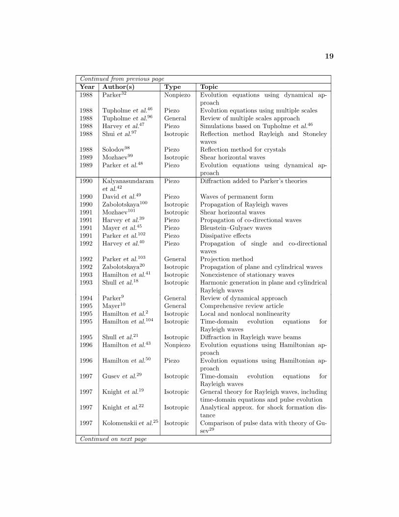
19
Continued from previous pageYear Author(s) Type Topic1988 Parker32 Nonpiezo Evolution equations using dynamical ap-
proach1988 Tupholme et al.46 Piezo Evolution equations using multiple scales1988 Tupholme et al.96 General Review of multiple scales approach1988 Harvey et al.47 Piezo Simulations based on Tupholme et al.46
1988 Shui et al.97 Isotropic Reflection method Rayleigh and Stoneleywaves
1988 Solodov98 Piezo Reflection method for crystals1989 Mozhaev99 Isotropic Shear horizontal waves1989 Parker et al.48 Piezo Evolution equations using dynamical ap-
proach1990 Kalyanasundaram
et al.42Piezo Diffraction added to Parker’s theories
1990 David et al.49 Piezo Waves of permanent form1990 Zabolotskaya100 Isotropic Propagation of Rayleigh waves1991 Mozhaev101 Isotropic Shear horizontal waves1991 Harvey et al.39 Piezo Propagation of co-directional waves1991 Mayer et al.45 Piezo Bleustein–Gulyaev waves1991 Parker et al.102 Piezo Dissipative effects1992 Harvey et al.40 Piezo Propagation of single and co-directional
waves1992 Parker et al.103 General Projection method1992 Zabolotskaya20 Isotropic Propagation of plane and cylindrical waves1993 Hamilton et al.41 Isotropic Nonexistence of stationary waves1993 Shull et al.18 Isotropic Harmonic generation in plane and cylindrical
Rayleigh waves1994 Parker9 General Review of dynamical approach1995 Mayer10 General Comprehensive review article1995 Hamilton et al.2 Isotropic Local and nonlocal nonlinearity1995 Hamilton et al.104 Isotropic Time-domain evolution equations for
Rayleigh waves1995 Shull et al.21 Isotropic Diffraction in Rayleigh wave beams1996 Hamilton et al.43 Nonpiezo Evolution equations using Hamiltonian ap-
proach1996 Hamilton et al.50 Piezo Evolution equations using Hamiltonian ap-
proach1997 Gusev et al.29 Isotropic Time-domain evolution equations for
Rayleigh waves1997 Knight et al.19 Isotropic General theory for Rayleigh waves, including
time-domain equations and pulse evolution1997 Knight et al.22 Isotropic Analytical approx. for shock formation dis-
tance1997 Kolomenskii et al.25 Isotropic Comparison of pulse data with theory of Gu-
sev29
Continued on next page
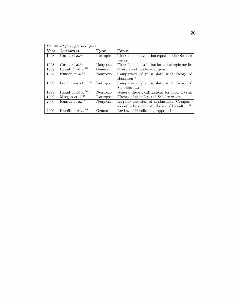
20
Continued from previous pageYear Author(s) Type Topic1998 Gusev et al.29 Isotropic Time-domain evolution equations for Scholte
waves1998 Gusev et al.29 Nonpiezo Time-domain evolution for anisotropic media1998 Hamilton et al.52 General Overview of model equations1998 Kumon et al.53 Nonpiezo Comparison of pulse data with theory of
Hamilton33
1999 Lomonosov et al.26 Isotropic Comparison of pulse data with theory ofZabolotskaya20
1999 Hamilton et al.52 Nonpiezo General theory, calculations for cubic crystal1999 Meegan et al.28 Isotropic Theory of Stoneley and Scholte waves2000 Kumon et al.54 Nonpiezo Angular variation of nonlinearity, Compari-
son of pulse data with theory of Hamilton33
2000 Hamilton et al.51 General Review of Hamiltonian approach
Chapter 2
Theory
This chapter describes the theory used throughout the rest of the dissertation.
First, the model equations for nonlinear SAWs in a nonpiezoelectric crystal
are reviewed. Second, approximate solutions to these equations are given,
and estimates for the shock formation distance and nonlinearity coefficient
are described. Third, a time-domain equation is derived corresponding to the
frequency-domain model equations presented in the first part of the chapter.
Finally, the theory for anisotropic media is compared in detail with the theory
of Zabolotskaya20 for nonlinear Rayleigh waves in isotropic media.
2.1 Description of the Model
The model employed here was developed by Hamilton, Il’inskii, and Zabolot-
skaya.33 Because their paper contains a step-by-step derivation of the model
equations, a description of the technique for their numerical solution, and a
detailed comparison to the isotropic case, only an overview of the theory is
given here.
2.1.1 Linear Theory
Because the linear theory forms the basis for the nonlinear theory, it is reviewed
first. From linear theory, the wave speed and ratios of particle displacement
components may be determined.
21
22
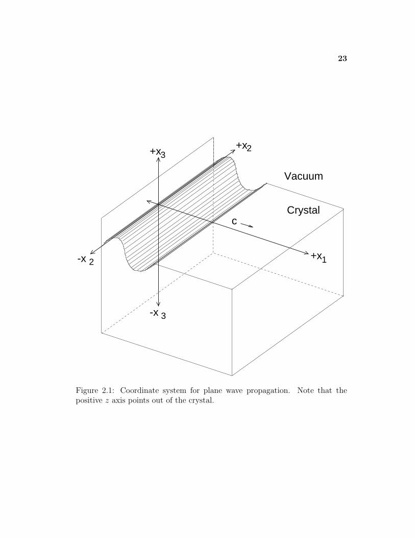
The coordinate system is selected such that the (x1, x2) plane coincides
with the surface of the crystal and the x3 axis is the outward normal to the
surface. The crystal occupies the half-space x3 ≤ 0 with a vacuum above.
Without loss of generality, the x1 axis is selected to be in the direction of
propagation (see Figure 2.1).
The equation of motion for the particle displacement ui as a function of
the stress tensor σij in a homogeneous elastic solid with density ρ is
ρ∂2ui
∂t2=
∂σij
∂xj, (2.1)
where the xj are the position variables, t is the time variable, and i, j ∈ {1, 2, 3}.The Einstein convention of summation over repeated indices is assumed. The
stress–strain relation to linear order in the strain for an arbitrary anisotropic
solid is
σij = cijklekl , (2.2)
where σij is the stress tensor,
eij =1
2
(∂ui
∂xj
+∂uj
∂xi
)(2.3)
is the linearized strain tensor, and cijkl are the second-order elastic (SOE)
constants. Substitution of Eqs. (2.3) and (2.2) into Eq. (2.1) yields the linear
wave equation
ρ∂2ui
∂t2= cijkl
∂2uk
∂xj∂xl
, (2.4)
written in terms of the displacement components.
To determine surface acoustic wave solutions of Eq. (2.4), consider in-
homogeneous plane wave solutions of the form
ui = αieik(l·x−ct) . (2.5)
23
c
+x
-x
+x
Vacuum
Crystal
-x
+x1
32
3
2
Figure 2.1: Coordinate system for plane wave propagation. Note that thepositive z axis points out of the crystal.
24
Here, the vector l = (l1, l2, l3) is defined such that l21 + l22 = 1. By choosing
the x1 axis to be the direction of propagation, it follows that l = (1, 0, ζ),
where ζ may be a complex number. For a wave with angular frequency ω, the
phase speed of this wave is c = ω/k and k is the corresponding wave number.
Substitution of Eq. (2.5) into Eq. (2.4) yields
ρc2αi = cijklljllαk . (2.6)
Here the SOE constants are defined with respect to the chosen set of coor-
dinates. Because the values of the SOE constants are usually provided with
respect to the coordinate system defined by the crystalline axes, a transforma-
tion must usually be performed. See Auld105 for a detailed discussion of this
procedure. Equation (2.6) has a nontrivial solution if
det[Γik(ζ)− ρc2δik] = 0 , (2.7)
where
Γik(ζ) = cijklljll (2.8)
and δik is the Kronecker delta function.
Equation (2.7) is a sixth-order algebraic equation in terms of ζ , and c is
a parameter of the equation. Because this equation has all real coefficients, its
roots must be real or complex conjugate pairs. The real solutions correspond to
bulk waves, whereas the complex solutions correspond to surface waves. Fur-
thermore, it is required that Im ζ < 0 for surface waves so that the amplitude
of the wave decays to zero as x3 → −∞. Three such roots exist for any value
of c. Hence the full solution of Eq. (2.4) has the form
ui =3∑
s=1
Csα(s)i eik(ls·x−ct) =
3∑s=1
Csα(s)i eiζskx3ei(kx1−ωt) , (2.9)
25
where ls = (l(s)1 , l
(s)2 , l
(s)3 ) = (1, 0, ζs). The coefficients Cs are determined by
substituting Eq. (2.9) into the stress-free boundary condition
σi3 = 0 at x3 = 0 (2.10)
to yield the condition
ci3kl
3∑s=1
Csα(s)k l
(s)l = 0 . (2.11)
Together Eqs. (2.7) and (2.11) allow for the solution of the real-valued wave
speed c, and complex-valued eigenvalues ζs, eigenvectors α(s)i , and coefficients
Cs. For an arbitrary anisotropic solid, these equations must be solved numeri-
cally. See Hamilton, et al.33 for a detailed discussion of the algorithm employed
to compute the results in this dissertation.
Several differences in physical motion occur between the isotropic and
anisotropic cases even in the linear approximation:
1. While the SAWs are still nondispersive in a crystalline half-space, their
wave speed c is no longer constant as a function of direction. See Fig. 4.1
for an example of this variation in selected cubic crystals.
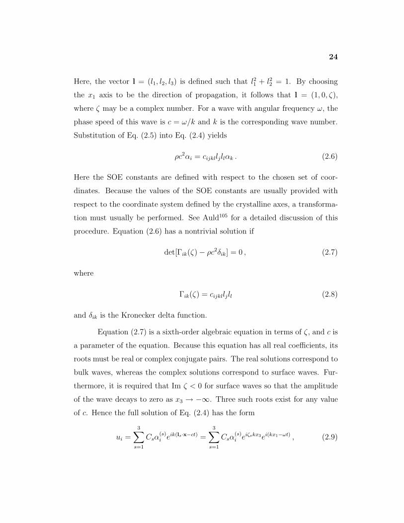
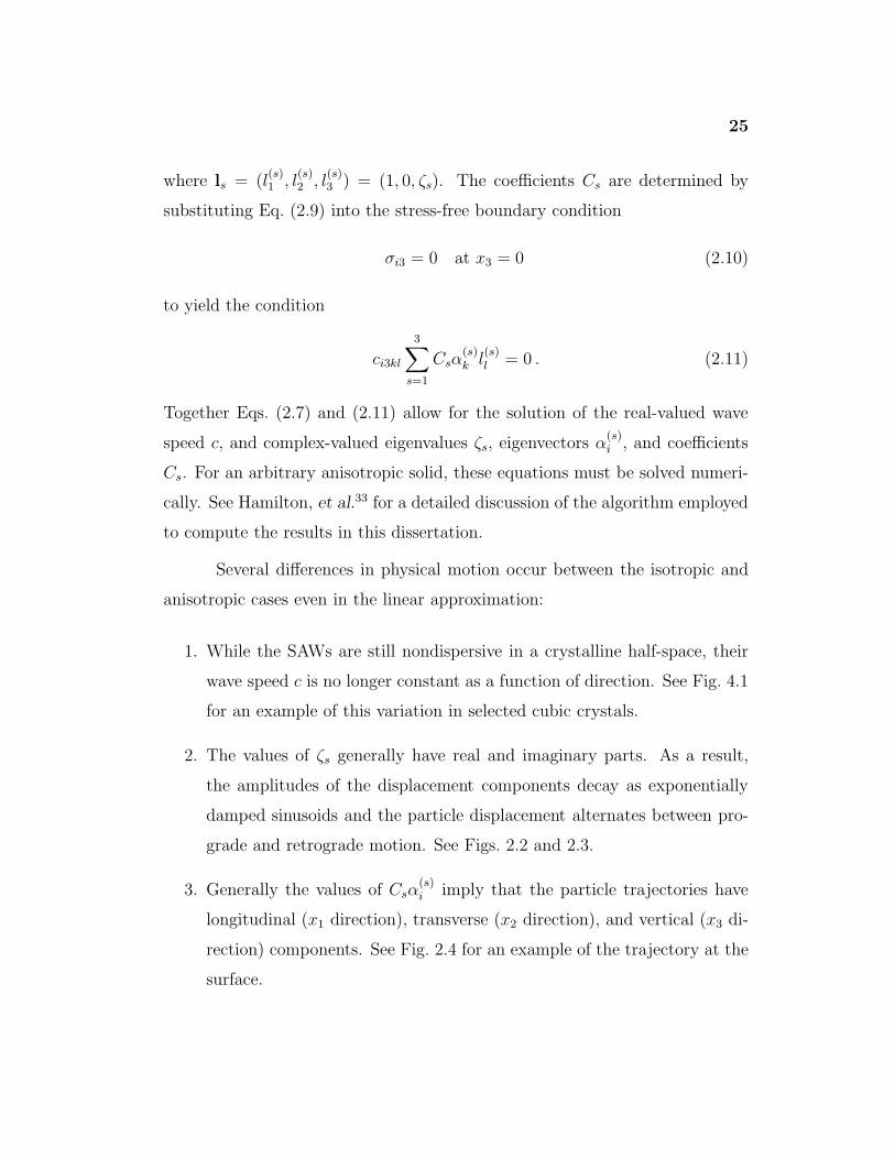
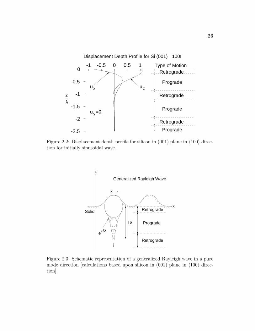
2. The values of ζs generally have real and imaginary parts. As a result,
the amplitudes of the displacement components decay as exponentially
damped sinusoids and the particle displacement alternates between pro-
grade and retrograde motion. See Figs. 2.2 and 2.3.
3. Generally the values of Csα(s)i imply that the particle trajectories have
longitudinal (x1 direction), transverse (x2 direction), and vertical (x3 di-
rection) components. See Fig. 2.4 for an example of the trajectory at the
surface.
26
-2.5
-2
-1.5
-1
-0.5
0-1 -0.5 0 0.5 1
⟨ ⟩
uz
λz−
uy=0
Retrograde
Prograde
Retrograde
Prograde
Retrograde
Prograde
Type of Motion
ux
100Displacement Depth Profile for Si (001)
Figure 2.2: Displacement depth profile for silicon in (001) plane in 〈100〉 direc-tion for initially sinusoidal wave.
k
Retrograde
x
z
Generalized Rayleigh Wave
Retrograde
Prograde
Solid
ez/λ
∼λ
Figure 2.3: Schematic representation of a generalized Rayleigh wave in a puremode direction [calculations based upon silicon in (001) plane in 〈100〉 direc-tion].
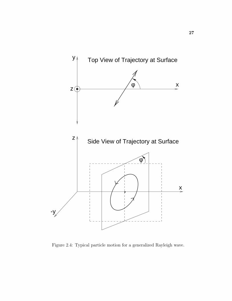
27
φ
-y
z
x
xφz
y Top View of Trajectory at Surface
Side View of Trajectory at Surface
Figure 2.4: Typical particle motion for a generalized Rayleigh wave.
28
4. In crystals, certain special directions can exist in which all values of ζs are
real and no surface wave solution occurs. Instead, there exists a trans-
versely polarized (x2 direction) bulk wave mode which satisfies the stress-
free surface boundary condition. Such a wave is called an exceptional or
surface-skimming bulk wave. See Fig. B.8 for a schematic diagram.
5. The group velocity is not generally coincident with the direction of the
phase velocity. Equivalently, the direction of power flow is not generally
coincident with the direction of the wave vector. Physically this implies
that the plane wave fronts are at an angle to the power flow direction.
Where the group and phase velocities are in the same direction, those
special cases are usually called pure modes.
See Farnell3 for a complete review of the linear properties of SAWs.
2.1.2 Nonlinear Theory
The method used to derive the nonlinear equations of motion is a generalization
of the method that was used to model SAWs in isotropic media by Zabolot-
skaya.20 It involves calculating the Hamiltonian at cubic order in the wave
variables, choosing appropriate generalized coordinates, applying the equations
of motion in canonical form, and deriving evolution equations for the slowly
varying amplitudes in a suitable retarded time frame. This method is very
general—it is applicable to a crystal of any symmetry for which the elastic
constants are known and to any cut and direction in such a crystal. Again,
only an outline of the key equations is given here.
To begin, the particle displacements for the plane SAWs were taken to
29
have the form
uj(x, z, t) =
∞∑n=−∞
an(t)unj(z)einkx , (2.12)
where
unj(z) =
3∑s=1
β(s)j einkζsz , (2.13)
unj = u∗(−n)j , β(s)j = Csα
(s)j , and j ∈ {1, 2, 3}. For simplicity, the notations x ≡
x1 and z ≡ x3 have been introduced in these expressions. Writing the solution
in this form assumes that the nonlinear solution is close to the linear solution; in
particular, the depth dependence unj at each frequency is the same as the linear
solution. It can be shown that nonlinear corrections to the depth dependence
are of higher order than the highest order terms kept in this model.28
Next, expressions for energy density of the crystal must be determined
in preparation for the computation of the system Hamiltonian. The elastic
energy per unit volume is
E =1
2cijkleijekl +
1
6dijklmneijeklemn + · · · , (2.14)
which corresponds to the nonlinear stress–strain relation
σij = cijklekl + cijklmneklemn , (2.15)
an extension of Eq. (2.2). In these equations the exact expression for the
Lagrangian strain tensor is
eij =1
2
(∂ui
∂xj+
∂uj
∂xi+
∂uk
∂xi
∂uk
∂xj
), (2.16)
where eij = eji, and the coefficients dijklmn are the third-order elastic (TOE)
constants. Substitution of Eq. (2.16) into Eq. (2.14) allows the energy density
to be written in terms of the quadratic and cubic contributions as
E = E2 + E3 , (2.17)
30
where
E2 =1
2cijkl
∂ui
∂xj
∂uk
∂xl
, (2.18)
E3 =1
6d′ijklmn
∂ui
∂xj
∂uk
∂xl
∂um
∂xn
, (2.19)
and
d′ijklmn = dijklmn + cijlnδkm + cjnklδim + cjlmnδik . (2.20)
The Hamiltonian of the system is constructed in the form
H = T + V + W , (2.21)
where T is the kinetic energy, V is the potential energy at quadratic order in the
particle displacement, and W is the potential energy at cubic order associated
with the nonlinear interactions. In terms of the particle displacement, these
quantities are given by
T =1
λ
∫ λ
0
dx
∫ 0
−∞
1
2ρu2
i dz , (2.22a)
V =1
λ
∫ λ
0
dx
∫ 0
−∞E2 dz , (2.22b)
W =1
λ
∫ λ
0
dx
∫ 0
−∞E3 dz , (2.22c)
where λ = 2π/k is the wavelength at the fundamental frequency in the Fourier
expansion of ui, the summation convention applies to u2i ≡ uiui, and ui =
dui/dt. The integration over z sums all the contributions of the energy from
the surface to infinite depth while the integration over x averages the expres-
sion over a region that is a characteristic wavelength in size. Substitution of
31
Eq. (2.12) into Eqs. (2.22) yields
T =ρ
2k
∑n
anan
|n| , (2.23a)
V =1
2ρc2k
∑n
|n|anan , (2.23b)
W = 3(W + W∗) , (2.23c)
where
W =∑
n1>0, n2>0,n3=−(n1+n2)
wn1n2n3an1an2an3 , (2.24)
wn1n2n3 = −k2
3
3∑s1,s2,s3=1
n1n2n3Fs1s2s3
n1ζs1 + n2ζs2 + n3ζs3
, (2.25)
Fs1s2s3 =1
2d′ijklmnβ
(s1)i β
(s2)k [β(s3)
m ]∗l(s1)j l
(s2)l [l(s3)
n ]∗ . (2.26)
In addition, the derivation of Eq. (2.23a) imposes the normalization condition
∫ 0
−∞
∣∣∣∣∣3∑
s=1
β(s)i eiζsz′
∣∣∣∣∣2
= 1 . (2.27)
Here again the values of the SOE and TOE constants in d′ijklmn must be trans-
formed into the coordinate system illustrated in Fig. 2.1.
To derive the equations of motion, generalized coordinates are selected
in order that Hamilton’s equations may be applied. The functions an are chosen
to be the generalized coordinates, and hence the generalized momenta are
pn =∂T
∂an=
ρ
k
a−n
|n| . (2.28)
Substituting Eqs. (2.21) and (2.23) into Hamilton’s canonical equations,
an =∂H
∂pn
, pn = −∂H
∂an
, (2.29)
32
then yields the amplitude equations for the system. The calculation may be
simplified without loss of accuracy by considering only progressive wave prop-
agation via the transformation
an =
{bne−inωt for n > 0b∗−ne−inωt for n < 0
, (2.30)
where the functions bn are slowly varying amplitude functions. However, the
desired form of the evolution equations are in terms of the velocity instead of
particle displacement. This can be achieved by defining
vn = an = −inωbn . (2.31)
The combination of the transformations defined by Eqs. (2.30) and (2.31) in
the evolution equations given by Eq. (2.29) yields
vn =n2ω
2ρc3
(n−1∑m=1
Sm,n−mvmvn−m − 2
∞∑m=n+1
S∗n,m−nvmv∗m−n
), (2.32)
for n > 0 and vn = v∗−n for n < 0. The nonlinearity matrix in this expression
is defined as
Slm =
3∑s1,s2,s3=1
Fs1s2s3
lζs1 + mζs2 − (l + m)ζ∗s3
, (2.33)
where Fs1s2s3 is defined by Eq. (2.26). Physically, the nonlinearity coefficients
Slm represent the strength of the coupling between the lth and mth to generate
the (l + m)th harmonic.
Equation (2.33) is useful for solving initial value problems. However,
often conditions are such that a boundary condition is specified instead of an
initial value condition, e.g., a known waveform is radiated from a source at
a given location. For these problems, the transformation from a temporal to
a spatial evolution equation has been shown19 to be equivalent to replacing
33
the temporal derivative vn with the spatial derivative c(dvn/dx). Under this
transformation, Eq. (2.32) becomes
dvn
dx=
n2ω
2ρc4
(n−1∑m=1
Sm,n−mvmvn−m − 2∞∑
m=n+1
S∗n,m−nvmv∗m−n
), (2.34)
for n > 0 and vn = v∗−n for n < 0. Physically, the first summation on the
right side represents sum frequency generation, while the second summation
represents difference frequency generation. The velocity waveforms are recon-
structed using
vj(x, z, t) =
∞∑n=1
vn(x)unj(z)ein(kx−ωt) + c.c. , (2.35)
where “c.c.” means “the complex conjugate of the previous term” and the
functions unj are given by Eq. (2.13). The expansion in Eq. (2.35) has no
n = 0 term because the bulk of the solid is assumed to be at rest. Because
Eq. (2.34) has no dissipative terms, the total energy of the wave33,41
E =∞∑
n=1
|vn|2n
(2.36)
must be conserved.
However, SAWs in real physical systems are attenuated by thermovis-
cous absorption. It has been shown that SAWs attenuate exponentially with
distance, and the decay coefficient is proportional to the frequency squared.106
This effect can be included in the model in an ad hoc fashion by adding the
term αnvn on the left side of Eq. (2.34)
dvn
dx+ αnvn =
n2ω
2ρc4
(n−1∑m=1
Sm,n−mvmvn−m − 2∞∑
m=n+1
S∗n,m−nvmv∗m−n
). (2.37)
where αn = n2α1 is the absorption coefficient for the nth harmonic. This
approach has been used previously for SAWs in isotropic media.18 Typically,
34
the absorption is chosen to be sufficiently weak that its primary effect is to
stabilize the portions of the waveform in the neighborhood of a shock without
significantly affecting the rest of the wave. In other words, the absorption acts
as high pass filter for the frequency components that give rise to the shock
front, but minimally attenuate the lowest frequency components that compose
the other parts of the wave.
The system of first-order differential equations of Eq. (2.37) must be
solved numerically. To accomplish this, it is convenient to introduce the di-
mensionless variables
Vn = vn/v0 , X = x/x0 , An = αnx0 , (2.38)
where v0 > 0 is a characteristic velocity of the SAW and
x0 =ρc4
4|S11|ωv0
(2.39)
is a length scale that characterizes the nonlinear distortion for a SAW radiated
at angular frequency ω with amplitude v0. Using these relations, it is possible
to rewrite the evolution equations in the form
dVn
dX+ AnVn =
n2
8|S11|
(n−1∑m=1
Sm,n−mVmVn−m − 2
N∑m=n+1
S∗n,m−nVmV ∗
m−n
).
(2.40)
For numerical purposes, only the first N harmonics are considered, so that only
N differential equations are integrated and the the series expansions are trun-
cated after N terms. The absorption coefficients An were added for purposes
of numerical stability as discussed above.
To integrate the system in Eq. (2.40) the boundary conditions must be
specified. The theoretical development listed above is general in the sense that
it applies for any set of initial spectral amplitudes. For the sake of simplicity,
35
now consider a specific example. It is common that the source condition be
given in terms of the time waveform at a fixed location. Suppose the source
is placed on the surface z = 0 at the position x = 0. Then by Eq. (2.35), the
velocity waveforms at the source may be expressed as
vj(0, 0, t) =
∞∑n=1
vn(0)Bje−inωt + c.c. , (2.41)
where
Bj =3∑
s=1
β(s)j . (2.42)
In much of the analysis and simulations that follows, a single frequency source
of angular frequency ω0 is used. In spectral form, this can be represented as
vn(0) =
v1 for n = 1v∗1 for n = −10 for n 6= ±1
, (2.43)
where v1 is generally complex and n = 1 corresponds to the fundamental an-
gular frequency ω. Applying Eq. (2.43) to Eq. (2.41) gives
vj(0, 0, t) = v∗1B∗j e
iωt + v1Bje−iωt = 2Re
[v1Bje
−iωt]
. (2.44)
If v1 = |v1| exp(iφv1) and Bj = |Bj| exp(iφBj), then Eq. (2.44) may be rewritten
as
vj(0, 0, t) = 2|v1||Bj| cos(ωt− φv1 − φBj) . (2.45)
The amplitudes |Bj| are determined by the normalization given in Eq. (2.27).
Only the relative phases |φBj−φBk| between the values of Bj and Bk are deter-
mined by solution of the linear problem; the absolute phase may be selected as
is convenient. As a result of Eq. (2.45), the amplitudes of the various velocity
components are given by the relations
|vx||vz| =
|B1||B3| ,
|vy||vz| =
|B2||B3| . (2.46)
36
Again, these equations only apply for a monofrequency source at the surface.
As an example, consider the case of an isotropic solid.107 For this class
of materials, monofrequency SAWs have only longitudinal and vertical compo-
nents, and the former leads the latter in phase by π/2. Choose the phase such
that B1 lies along the negative imaginary axis and, therefore, φB1 = −π/2 and
φB3 = 0 (φB2 is undefined because B2 = 0).∗ Furthermore, suppose v1 = |v0|so that φv1 = 0. Then Eq. (2.45) becomes†
vx(0, 0, t) = 2v0|B1| cos(ωt + π/2) = −2v0|B1| sinωt , (2.47a)
vz(0, 0, t) = 2v0|B3| cos ωt . (2.47b)
Similarly, suppose v1 = −|v0| < 0 so that φv1 = π. Then Eq. (2.45) becomes
vx(0, 0, t) = 2|v0||B1| cos(ωt− π + π/2) = 2|v0||B1| sinωt , (2.48a)
vz(0, 0, t) = 2|v0||B3| cos(ωt− π) = −2|v0||B3| cos ωt . (2.48b)
Thus, if vx(0, 0, t) = vx0 sin ωt, then in both cases the amplitude of the time
waveform may be related to the spectral amplitude by
v1 = − vx0
2|B1| . (2.49)
Note again that the results of this paragraph apply only on the surface and at
the source in an isotropic solid.
∗In contrast, Landau and Lifshitz107 select the phase such that the equivalent of B1 liesalong the negative real axis.
†Except for the early papers by Zabolotskaya20,100 on the theory for Rayleigh waves,subsequent papers employing the same approach2,18,19,21,22,41,104 use a series expansion forvj that contains a prefactor of 1/2, and hence the expression corresponding to this equationdoes not contain the factor of 2 [see Eq. (14) in Shull et al.18].
37
2.2 Approximate Solutions
Approximate analytical solutions of Eq. (2.40) may be obtained by considering
only second harmonic generation due to the fundamental frequency term. Con-
sider the monofrequency source of Eq. (2.43). Let the characteristic velocity be
v0 = |v1| so that in nondimensional form the source condition takes the form
Vn(0) =
{e±iφv for n = ±10 for n 6= ±1
, (2.50)
where eiφv = v1/|v1|.
2.2.1 Quasilinear Solution
First consider Eq. (2.40) for N = 1 in the linear approximation:
dV1
dX+ A1V1 = 0 . (2.51)
Solving this equation subject to Eq. (2.50) yields
V1 = eiφve−A1X . (2.52)
Next consider Eq. (2.40) for the second harmonic but only retain the terms on
the right side corresponding to the fundamental:
dV2
dX+ A2V2 =
S11
2|S11|V21 . (2.53)
Solving this equation using Eq. (2.50) and Eq. (2.52) yields
V2 =S11e
2iφv
2|S11|e−2A1X − e−A2X
A2 − 2A1
. (2.54)
Recall that S11 is complex-valued, and so most generally S11/|S11| = eiφS11 for
some phase factor∗ 0 ≤ φS11 ≤ 2π. Close to the source (X � 1), Eq. (2.52)
∗As shown in Chapter 6, the phase of the nonlinearity matrix elements plays an importantrole in determining how the waveform distorts.
38
and Eq. (2.54) can be approximated by the Taylor series expansions
V1 = eiφv
[1− A1X +
1
2A2
1X2 + O(X3)
], (2.55a)
V2 =S11e
2iφv
2|S11|[X − 1
2A′X2 +
1
6A′′X3 + O(X4)
], (2.55b)
where A′ = 2A1 + A2 and A′′ = 4A21 + 2A1A2 + A2
2. In the limit that the
absorption coefficients A1, A2 → 0, Eqs. (2.55) reduce to
V1 = eiφv , (2.56a)
V2 =S11e
2iφv
2|S11| X . (2.56b)
In dimensional form, the magnitudes of the harmonics are then
|v1|v0
= 1 , (2.57a)
|v2|v0
=x
2x0. (2.57b)
Hence within this approximation the second harmonic increases linearly with
range, just as both Rayleigh waves and longitudinal bulk waves in lossless media
do in the nonlinear regime. A weakness of this solution is that the fundamental
does not decrease, clearly violating energy conservation. An improved approx-
imation is given in Section 2.2.3.
2.2.2 Estimates of Nonlinearity Parameters
This similarity of Eq. (2.57b) with bulk waves in lossless fluids makes it possible
to derive an estimate of the shock formation distance. Let xl be the shock
formation distance for a finite amplitude sound wave in a lossless medium
radiated at angular frequency ω and velocity amplitude v0. The quasilinear
solution of the amplitude of the second harmonic component in the fluid then
39
may be expressed as108
|v2|v0
=x
2xl
. (2.58)
Comparison of Eq. (2.58) and the amplitude of Eq. (2.57b) shows that an
estimate of the shock formation distance x11 in the SAW is
x11 = x0 =ρc4
4|S11|ωv0
. (2.59)
As would be expected, x11 depends on the TOE constants via the nonlinearity
matrix element S11. In addition, the shock formation depends inversely on
the strength of the nonlinearity, wave amplitude, and frequency. However, the
amplitude of the time waveform more typically is known from experiment, not
the spectral amplitude. Hence Eq. (2.59) may be rewritten using Eq. (2.49) to
yield
xx011 =
|B1|ρc4
2|S11|ω|vx0| . (2.60)
Equation (2.59) and Eq. (2.60) are equivalent; the latter is given here primarily
for purposes of convenience.
Equation (2.59) has several limitations. First, it is limited in accuracy.
It only contains one term (|S11|) that describes the strength of the nonlinear-
ity, and this factor characterizes only the energy transfer from the fundamental
to the second harmonic. Generation of higher harmonics is necessary for the
formation of a shock, but these harmonics are not accounted for Eq. (2.59).
Second, there exist cases where harmonic generation occurs but shock forma-
tion does not, e.g., near the 〈100〉 direction in the (001) cut of KCl33 (see also
Section 4.2.3). Thus the estimate given by Eq. (2.59) is no longer meaningful.
This limitation is related to the first one because (at least for the KCl case) it
is the low coupling strength of the fundamental to the harmonics higher than
40
second that prevents the shock from forming. Lastly, Eq. (2.59) was derived
assuming a source with a clearly defined angular frequency ω and amplitude
v0. However, it is more common experimentally to have pulses with a range
of spectral amplitudes. While it is possible to apply Eq. (2.59) to this situa-
tion by selecting a characteristic frequency and amplitude for the pulse, this is
essentially an approximation within an approximation. Despite these limita-
tions, Eq. (2.59) provides at least a first-order estimate of the shock formation
distance for many cases of interest and is still useful in this respect. (See Sec-
tion 2.4.3 for comparison of this estimate to the estimates for isotropic solids.)
An expression for the effective coefficient of nonlinearity also may be
derived by drawing an analogy to bulk waves in lossless media. For a finite-
amplitude wave of angular frequency ω and amplitude vl propagating in such
a medium, the shock formation distance xl is related to the coefficient of non-
linearity βl by108
xl =1
|βl|εlk, (2.61)
where εl = vl/c is the acoustic Mach number and k = ω/c is the wave number.
Eq. (2.59) may be rewritten as
x11 =1∣∣∣4S11
ρc2
∣∣∣ v0
cωc
=1
|β|εk . (2.62)
Hence the coefficient of nonlinearity is identified as
β = −4S11
ρc2(2.63)
and depends on the TOE constants, as would be expected, through S11. In
general, β is complex-valued, although cases do exist where it is strictly real-
valued. The negative sign is introduced in Eq. (2.63) so that the sign of the
nonlinearity coefficient is consistent with the theory for isotropic materials of
41
Zabolotskaya20 (see Sections 2.4.2 and 2.4.3 for further discussion). Because
Eq. (2.62) is derived from Eq. (2.59), its limitations are the same as those
discussed in the previous paragraph. (See Section 2.4.3 for comparison of this
estimate to the estimates for isotropic solids.)
Because the definition of the coefficient of nonlinearity is given relative
to a characteristic velocity, different characteristic velocities can give rise to
different expressions for the coefficient of nonlinearity for the same estimate of
the shock formation distance. For example, Eq. (2.60) can be rewritten as
xx011 =
1∣∣∣ 2S11
ρc2|B1|
∣∣∣ |vx0|c
ωc
=1
|βx0||εx0|k , (2.64)
where εx0 = vx0/c is the longitudinal acoustic Mach number. In this formula-
tion, the coefficient of nonlinearity
βx0 = − 2S11
ρc2|B1| (2.65)
is defined relative to the characteristic velocity vx0. Again, the negative sign
is introduced for purposes of consistency. Note that while x11 = xx011 , βx0 6= β
and vx0 6= v0. As described previously, Eq. (2.65) may be more convenient for
practical purposes.
2.2.3 Tapered Quasilinear Solution
One of the disadvantages of the quasilinear solution given by Eq. (2.52) and
Eq. (2.54) is that it does not account for decrease in the amplitude of the
fundamental by transfer of energy to the second harmonic. The approach of
Merklinger109 for finite amplitude waves in fluids, as extended by Shull et al.18
for Rayleigh waves in isotropic solids, may be used to approximate this deple-
tion. Suppose the first harmonic component may be written in nondimensional
42
form as
V1 = T1(X)V1 , (2.66)
where T1 is the taper function that accounts for the decrease in V1 due to
harmonic generation. By the boundary condition Eq. (2.50), V1(0) = eiφv , and
by Eq. (2.52), V1(0) = eiφv . Hence T1(0) = 1 is the appropriate boundary
condition for the taper function. The solution for the second harmonic given
by Eq. (2.54) derives from the forcing function proportional to V 21 on the right
side of Eq. (2.53). Hence the second harmonic term can be approximated by
taking
V2 = T 21 (X)V2 (2.67)
in this modified solution. Consider Eq. (2.40) with N = 2 and n = 1:
dV1
dX+ A1V1 = −1
4
S∗11
|S11| V∗1 V2 . (2.68)
Substitution of Eqs. (2.66) and (2.67) into Eq. (2.68) and simplification via
Eqs. (2.51) and (2.52) yield
dT1
dX= −e−2iφv
4
S∗11
|S11|T∗1 T 2
1 V2 . (2.69)
Substitution of Eq. (2.54) into Eq. (2.69) gives
dT1
dX= −1
8T ∗
1 T 21
e−2A1X − e−A2X
A2 − 2A1
. (2.70)
Let T1(X) = |T1(X)|eiφT (X) where |T1(X)| and φT (X) are real-valued functions.
Then Eq. (2.70) becomes
d|T1|dX
+ i|T1|dφT
dX= −1
8|T1|3 1
A2 − 2A1
(e−2A1X − e−A2X
). (2.71)
Because the right side of this equation is real-valued, it follows that dφT/dX =
0, and hence φT (X) = φT0 = const. The full taper function then has the form
43
T1(X) = |T1(X)|eiφT0 . But by the boundary condition T (0) = 1, it then follows
that φT0 = 0 and T1(X) = |T1(X)|. By separation of variables, the remaining
real part of Eq. (2.71) may be shown to have the solution
T1 = |T1| =[1 +
1
8A1A2
(1− A2e
−2A1X − 2A1e−A2X
A2 − 2A1
)]−1/2
. (2.72)
This equation indicates that if A1A2 � 1, then the nonlinear effects on the
fundamental are negligible because T1 ≈ 1 in that regime. The complete solu-
tion in terms of the velocity amplitude is then given by substituting Eq. (2.72)
into Eqs. (2.66) and (2.67):
V1 = T1(X)eiφve−A1X , (2.73a)
V2 = T 21 (X)
S11e2iφv
2|S11|e−2A1X − e−A2X
A2 − 2A1. (2.73b)
Close to the source (X � 1), these solutions can be approximated by the
Taylor series expansions
V1 = eiφv
[1− A1X +
(1
2A2
1 −1
16
)X2 + O(X3)
], (2.74a)
V2 =S11e
2iφv
2|S11|[X − 1
2A′X2 +
(1
6A′′ − 1
8
)X3 + O(X4)
], (2.74b)
where A′ = 2A1 + A2 and A′′ = 4A21 + 2A1A2 + A2
2 as before. Equations (2.74)
are analogous to Eqs. (2.55) in the non-tapered case. In the limit that the
absorption coefficients A1, A2 → 0, Eqs. (2.74) reduce to
V1 = eiφv
[1− 1
16X2
], (2.75a)
V2 =S11e
2iφv
2|S11|[X − 1
8X3 +
1
256X5
]. (2.75b)
Equations (2.75) are analogous to Eqs. (2.56) in the non-tapered case. Note
that, even in the absence of absorption, the fundamental exhibits a decrease
in amplitude away from the source. Correspondingly, the linear increase in
44
the second harmonic is decreased by the cubic term relative to the non-taper
compensated case. Again, these Taylor series results only apply near to the
source and neglect interactions with all other higher harmonics.
The nonlinear processes in other regimes can be investigated by taking
other limits. Consider the situation where the wave has propagated more than
its shock formation distance (X > 1) but less than the small-signal absorption
length (A1X < 1). Equations (2.73) can then be rewritten as
V1 =
[1 +
1
8X2 − 2A1 + A2
24X3 + O(X4)
]−1/2
V1 , (2.76a)
V2 =
[1 +
1
8X2 − 2A1 + A2
24X3 + O(X4)
]−1
V2 , (2.76b)
where the taper function has been expanded into a Taylor series about X = 0.
Next, suppose the small-signal absorption of the fundamental is sufficiently
small as compared to the nonlinear depletion of the fundamental by energy
transfer to higher harmonics (with the resulting higher absorption at those
higher frequencies) so that the absorption can be neglected. In this approxi-
mation, Eqs. (2.76) combined with Equations (2.56) become
V1 =eiφv√
1 + X2/8, (2.77a)
V2 =S11e
2iφv
2|S11|X
1 + X2/8. (2.77b)
Suppose also that X2 � 1 so that Eqs. (2.77) can be approximated as
V1 ∼ eiφv2√
2
X, (2.78a)
V2 ∼ S11e2iφv
2|S11|8
X. (2.78b)
Eqs. (2.78) are then valid in the range 1 � X2 � A−21 . Converting back to
45
dimensional variables via Eqs. (2.38), Eqs. (2.78) become
v1 ∼ eiφv
√2
ρc3
|S11|kx, (2.79a)
v2 ∼ S11e2iφv
|S11|ρc3
|S11|kx(2.79b)
Hence the velocity amplitudes in this region are independent of the source
amplitude v0. This phenomenon is known as acoustical saturation and is well-
known in nonlinear acoustics.110 Physically, the effect can be explained in the
following way. In this parameter regime, any increase in the source ampli-
tude does not cause an increase in the received amplitude at a fixed location.
Instead, the extra acoustic energy causes shocks to form closer to the source.
The additional dissipation that results offsets the increase in the amplitude that
would be predicted at that location by linear theory. This effect has been de-
scribed theoretically by Shull et al.18 for Rayleigh waves and has been observed
experimentally in LiNbO3.34,60,69
Finally, consider the “old age” region that is many absorption lengths
(A1X � 1) from the source. In this regime, the velocity amplitude of the
fundamental given in Eq. (2.73) becomes
V1 ∼[1 +
1
8A1A2
]−1/2
eiφve−A1X . (2.80)
Assuming that the source amplitude is sufficiently large that shocks form
(A1A2 � 1)∗, this may be further approximated as
V1 ∼√
8A1A2eiφve−A1X . (2.81)
∗Note that in the case of quadratic absorption, the condition for shock formation becomesA1 � 1/2 or 1/A1 � 2. Because 1/A1 = 1/α1x0 = 4|S11|ωv0/ρc4α1 is a parameter whichcharacterizes the ratio of nonlinear to thermoviscous effects, this indicates that nonlineareffects are dominant, as expected. Here then 1/A1 is the analogue of the Gol’dberg numberΓ in fluids.108
46
In dimensional form, this equation has the form
v1 ∼ ρc3
√2|S11|k
eiφve−α1x , α1α2 � 1
x20
=
(4|S11|ωv0
ρc4
)2
. (2.82)
In this region, the amplitude of the wave is proportional to e−α1x as predicted
by linear theory, but is also much further reduced in amplitude due to the
additional dissipation at the shock. The amplitude is again independent of the
source velocity and the small-signal absorption dominates the nonlinear effects.
2.2.4 Coupled Two-Mode Solution
The analysis with the taper function assumes that the propagation of the finite-
amplitude SAW is “typical,” i.e., it exhibits harmonic generation and shock
formation. However, as mentioned briefly above, there exist special cases where
this is not true. Consider the case of propagation near the 〈100〉 direction in
the (001) cut of KCl (see Section 4.2.3). As has been shown,33 shock formation
does not occur in this case because the magnitude of S12 is more than an order
of magnitude smaller than other “neighboring” elements like S11 and S13. As
a result, the generation of the third harmonic is sufficiently inefficient that
shocks do not form. This “trapping” of energy in the fundamental and second
harmonic allows a simpler set of model equations to describe the nonlinear
interactions, at least close to the source.33 Truncating Eqs. (2.40) at N = 2
in the absence of absorption yields the nonlinear, coupled system of equations
that take the form
dV1
dX= − S∗
11
4|S11|V∗1 V2 , (2.83a)
dV2
dX=
S∗11
2|S11|V21 . (2.83b)
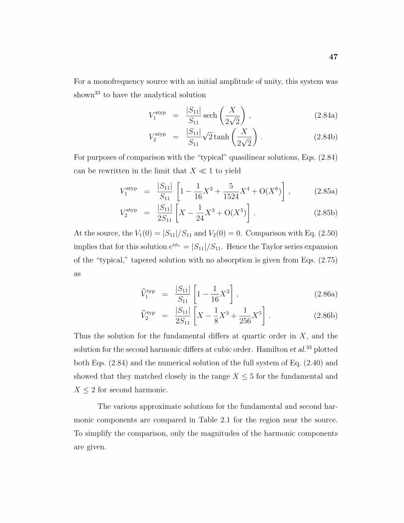
47
For a monofrequency source with an initial amplitude of unity, this system was
shown33 to have the analytical solution
V atyp1 =
|S11|S11
sech
(X
2√
2
), (2.84a)
V atyp2 =
|S11|S11
√2 tanh
(X
2√
2
). (2.84b)
For purposes of comparison with the “typical” quasilinear solutions, Eqs. (2.84)
can be rewritten in the limit that X � 1 to yield
V atyp1 =
|S11|S11
[1− 1
16X2 +
5
1524X4 + O(X6)
], (2.85a)
V atyp2 =
|S11|2S11
[X − 1
24X3 + O(X5)
]. (2.85b)
At the source, the V1(0) = |S11|/S11 and V2(0) = 0. Comparison with Eq. (2.50)
implies that for this solution eiφv = |S11|/S11. Hence the Taylor series expansion
of the “typical,” tapered solution with no absorption is given from Eqs. (2.75)
as
V typ1 =
|S11|S11
[1− 1
16X2
], (2.86a)
V typ2 =
|S11|2S11
[X − 1
8X3 +
1
256X5
]. (2.86b)
Thus the solution for the fundamental differs at quartic order in X, and the
solution for the second harmonic differs at cubic order. Hamilton et al.33 plotted
both Eqs. (2.84) and the numerical solution of the full system of Eq. (2.40) and
showed that they matched closely in the range X ≤ 5 for the fundamental and
X ≤ 2 for second harmonic.
The various approximate solutions for the fundamental and second har-
monic components are compared in Table 2.1 for the region near the source.
To simplify the comparison, only the magnitudes of the harmonic components
are given.
48
With absorptionType |V1| |V2|QL 1− A1X + 1
2A2
1X2 + O(X3) X − 1
2A′X2 + 1
6A′′X3 + O(X4)
TQL 1− A1X + (12A2
1 − 116
)X2 X − 12A′X2 +
(16A′′ − 1
8
)X3
+O(X3) +O(X4)
Without absorptionType |V1| |V2|QL 1 X
TQL 1− 116
X2 X − 18X3 + 1
256X5
C2M 1− 116
X2 + 51524
X4 + O(X6) X − 124
X3 + O(X5)
Table 2.1: Comparison of various approximate solutions of the spectral evo-lution equations for the fundamental and second harmonic near the source.A monofrequency source function of angular frequency ω is assumed andA′ = 2A1 +A2 and A′′ = 4A2
1 +2A1A2 +A22. The solution types are quasilinear
(QL), tapered quasilinear (TQL), and coupled two-mode (C2M).
49
2.3 Time-Domain Evolution Equation
A time-domain equation for the evolution of nonlinear SAWs on the surface of
crystals (x3 = 0) may be derived from the frequency-domain evolution equation
in Eq. (2.34). For convenience, Eq. (2.34) may be rewritten with the summation
on the right side performed over all indices, both positive and negative:
dvn
dx=
n2ω0
2ρc4
∑l+m=n
lm
|lm|Slm(−n)vlvm , (2.87)
where ω0 is the angular frequency of the fundamental. From Eq. (2.35), the
velocity component in the xi direction can be similarly rewritten as
vi(x, z, τ) =∞∑
n=−∞vn(x)uni(z)e−inω0τ , (2.88)
where the depth functions uni are given by Eq. (2.13), τ = t − x/c, and ω0 =
2π/T is the angular frequency associated with the waveform of period T . (Note
that the spectral component with n = 0 is zero because the bulk of the solid is
assumed to be at rest.) At the surface, Eq. (2.88) reduces to
vi(x, τ) =
∞∑n=−∞
vn(x)unie−inω0τ , (2.89)
where
uni =
{Bi =
∑3s=1 β
(s)i for n > 0
B∗i =
∑3s=1(β
(s)i )∗ for n < 0
}= |Bi|ei(n/|n|)φBi . (2.90)
Differentiating Eq. (2.89) with respect to x and substituting Eq. (2.87) into the
resulting equation yields
∂vi
∂x=
ω0
2ρc4
∞∑n=−∞
n2unie−inω0τ
∑l+m=n
lm
|lm|Slm(−n)vlvm . (2.91)
50
Equation (2.89) can be inverted by multiplying both sides by einω0τ and inte-
grating over a period. The result is
vn(x) =ω0
2πuni
∫ T/2
−T/2
vi(x, τ) dτ . (2.92)
Substituting Eq. (2.92) into Eq. (2.91) gives
∂vi
∂x=
ω20
4π2c2
1
2ρc2
∞∑n=−∞
(−inω0)(inuni)e−inω0τ
∑l+m=n
lm
|lm|uliumiSlm(−n)
×∫ T/2
−T/2
∫ T/2
−T/2
vi(x, τ1)vi(x, τ2)eilω0τ1eimω0τ1 dτ1 dτ2 .
(2.93)
Identifying (−inω0) with ∂/∂τ , applying the constraint n = l + m to the first
summation, and letting T = 2π/ω0 yields
∂vi
∂x=
CS
c2T 2
∂
∂τ
∫ T/2
−T/2
∫ T/2
−T/2
LS(φBi, τ − τ1, τ − τ2)vi(x, τ1)vi(x, τ2) dτ1 dτ2 ,
(2.94)
where CS = −1/2ρc2|Bi|. The kernel of the integral
LS(φBi, τ1, τ2) =∞∑
l=−∞
∞∑m=−∞
Plm(φBi)Qlm(φBi)Slme−ilω0τ1e−imω0τ2 , (2.95)
where
Plm(φ) = i(l + m)eiφ(l+m)/|l+m| , (2.96a)
Qlm(φ) = − lm
|lm|e−iφl/|l|e−iφm/|m| . (2.96b)
As mentioned in Section 2.1.2, linear theory only fixes the relative phases of the
Bi. Hence without loss of generality, one component can always be chosen such
that Bi0 = −|Bi0 |i = |Bi0|e−iπ/2, i.e., the absolute phase φBi0 = −π/2. Under
this condition, the kernel for the particular velocity component vi0 reduces to
LS(φBi0 = −π/2, τ1, τ2) =
∞∑l=−∞
∞∑m=−∞
|l + m|Slme−ilω0τ1e−imω0τ2 , (2.97)
51
as shown in Section 2.4.4.
Other velocity components vj(x, τ) (j 6= i) may be obtained from inte-
gral transforms of the vi(x, τ) component. The discrete Fourier transform of
vj(x, τ) is
vj(x, τ) =
∞∑n=−∞
vjn(x)e−inω0τ . (2.98)
From Eqs. (2.89) and (2.90), it follows that the nth spectral amplitudes of the
jth and ith velocity components are related by
vjn(x) =
{(Bj/Bi)vin(x) for n > 0(B∗
j /B∗i )vin(x) for n < 0
. (2.99)
Equation (2.99) implies that the velocity waveform components in the xj and
xi directions are related by31
vj(x, τ) = Re(Bj/Bi)vi(x, τ)− Im(Bj/Bi)H[vi(x, τ)] , (2.100)
where
H(f(τ)) =1
πPr
∫ ∞
−∞
f(τ ′)τ ′ − τ
dτ ′ (2.101)
defines the Hilbert transform ,111 Re(z) is the real part of a complex number z,
Im(z) is the imaginary part of a complex number z, and Pr means the Cauchy
principal value of the integral.112 A detailed proof of this relation is given in
Appendix E.
2.4 Comparison with Isotropic Solids
The purpose of this section is to provide a comparison of the theory of Zabolot-
skaya20 for isotropic media (also Hamilton et al.,2,41,104 Shull et al.,18,21 and
52
Knight et al.19,22) with the theory of Hamilton et al.33,43 for anisotropic me-
dia. The anisotropic theory has been shown to reduce to the isotropic theory
in the limit that the material constants correspond to isotropic symmetry,33
but various other differences in notion and notation exist in the various papers
describing the theories. The analysis in this section explicitly examines these
differences.
2.4.1 Linear Solution
The linear solution for the velocity components of a Rayleigh wave of angular
frequency ω and wave number k is given by [Shull et al.18 based on Eqs. (1)
and (2)]
vx(x, z, t) = iI(ξteξtkz + ηeξlkz)ei(kx−ωt) + c.c. , (2.102a)
vz(x, z, t) = I(eξtkz + ξlηeξlkz)ei(kx−ωt) + c.c. , (2.102b)
where
ξt = (1− ξ2)1/2 , (2.103a)
ξl = (1− ξ2c2t/c
2l )
1/2 , (2.103b)
η = −2(1− ξ2)1/2/(2− ξ2) , (2.103c)
ξ = cR/ct , (2.103d)
ξ6 − 8ξ4 + 8ξ2
(3− 2
c2t
c2l
)− 16
(1− c2
t
c2l
)= 0 , (2.103e)
cl is the phase speed of longitudinal bulk waves, ct is the phase speed of trans-
verse bulk waves, cR = ω/k is the Rayleigh wave speed, and I is the appropriate
amplitude to match the boundary conditions at the source. Note that ξ, ξt, ξl,
and η are solely functions of ct/cl. The linear solution for the velocity wave-
forms of a generalized Rayleigh wave under the same conditions is [Hamilton et
53
al.,33 Eqs. (74) and (75); Eq. (2.35) with Eq. (2.13) here]
vx(x, z, t) = A
(3∑
s=1
β(s)1 eikζsz
)ei(kx−ωt) + c.c. , (2.104a)
vz(x, z, t) = A
(3∑
s=1
β(s)3 eikζsz
)ei(kx−ωt) + c.c. , (2.104b)
where A is the appropriate amplitude to match the boundary conditions at
the source. Because of the isotropic symmetry, the wave number representing
the two transverse decay modes is degenerate. Suppose then that ζ1 = ζ2 are
the penetration depth parameters corresponding to ξt and ζ3 is the penetration
depth parameter corresponding to ξl. With these assumptions Eq. (2.104) can
be rewritten
vx(x, z, t) = A[(β
(1)1 + β
(2)1 )eikζ1z + β
(3)1 eikζ3z
]ei(kx−ωt) + c.c. ,(2.105a)
vz(x, z, t) = A[(β
(1)3 + β
(2)3 )eikζ1z + β
(3)3 eikζ3z
]ei(kx−ωt) + c.c. .(2.105b)
Because Eqs. (2.102) and Eqs. (2.105) must give the same result, the various
coefficients must be equivalent. A comparison of these coefficients is given in
Table 2.2.
2.4.2 Nonlinear Solution
Because an explicit comparison of the nonlinear theories for SAWs in isotropic
and anisotropic solids is given in Appendix B of Hamilton et al.,33 the com-
parison given here only introduces the notation and results needed for subse-
quent sections. The velocity components of the series expansions describing
the Rayleigh waves have the form [Shull et al.,18 Eqs. (1)–(4)]
vx(x, z, t) =1
2
∞∑n=−∞
vn(x)uxn(z)ein(kx−ωt) , (2.106a)
vz(x, z, t) =1
2
∞∑n=−∞
vn(x)uzn(z)ein(kx−ωt) , (2.106b)
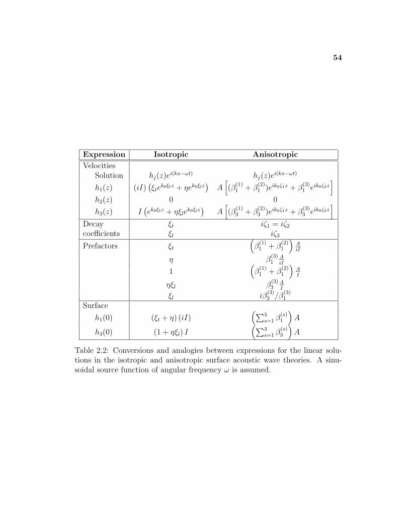
54
Expression Isotropic Anisotropic
VelocitiesSolution hj(z)ei(kx−ωt) hj(z)ei(kx−ωt)
h1(z) (iI)(ξte
k0ξtz + ηek0ξlz)
A[(β
(1)1 + β
(2)1 )eik0ζ1z + β
(3)1 eik0ζ3z
]h2(z) 0 0
h3(z) I(ek0ξtz + ηξle
k0ξlz)
A[(β
(1)3 + β
(2)3 )eik0ζ1z + β
(3)3 eik0ζ3z
]Decay ξt iζ1 = iζ2
coefficients ξl iζ3
Prefactors ξt
(β
(1)1 + β
(2)1
)AiI
η β(3)1
AiI
1(β
(1)1 + β
(2)1
)AI
ηξl β(3)3
AI
ξl iβ(3)3 /β
(3)1
Surface
h1(0) (ξt + η) (iI)(∑3
s=1 β(s)1
)A
h3(0) (1 + ηξl) I(∑3
s=1 β(s)3
)A
Table 2.2: Conversions and analogies between expressions for the linear solu-tions in the isotropic and anisotropic surface acoustic wave theories. A sinu-soidal source function of angular frequency ω is assumed.
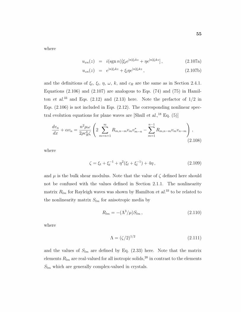
55
where
uxn(z) = i(sgn n)[ξte|n|ξtkz + ηe|n|ξlkz] , (2.107a)
uzn(z) = e|n|ξtkz + ξlηe|n|ξlkz , (2.107b)
and the definitions of ξt, ξl, η, ω, k, and cR are the same as in Section 2.4.1.
Equations (2.106) and (2.107) are analogous to Eqs. (74) and (75) in Hamil-
ton et al.33 and Eqs. (2.12) and (2.13) here. Note the prefactor of 1/2 in
Eqs. (2.106) is not included in Eqs. (2.12). The corresponding nonlinear spec-
tral evolution equations for plane waves are [Shull et al.,18 Eq. (5)]
dvn
dx+ αvn =
n2µω
2ρc4Rζ
(2
∞∑m=n+1
Rm,n−mvmv∗m−n −n−1∑m=1
Rm,n−mvmvn−m
),
(2.108)
where
ζ = ξt + ξ−1t + η2(ξl + ξ−1
l ) + 4η , (2.109)
and µ is the bulk shear modulus. Note that the value of ζ defined here should
not be confused with the values defined in Section 2.1.1. The nonlinearity
matrix Rlm for Rayleigh waves was shown by Hamilton et al.33 to be related to
the nonlinearity matrix Slm for anisotropic media by
Rlm = −(Λ3/µ)Slm , (2.110)
where
Λ = (ζ/2)1/2 (2.111)
and the values of Slm are defined by Eq. (2.33) here. Note that the matrix
elements Rlm are real-valued for all isotropic solids,20 in contrast to the elements
Slm which are generally complex-valued in crystals.
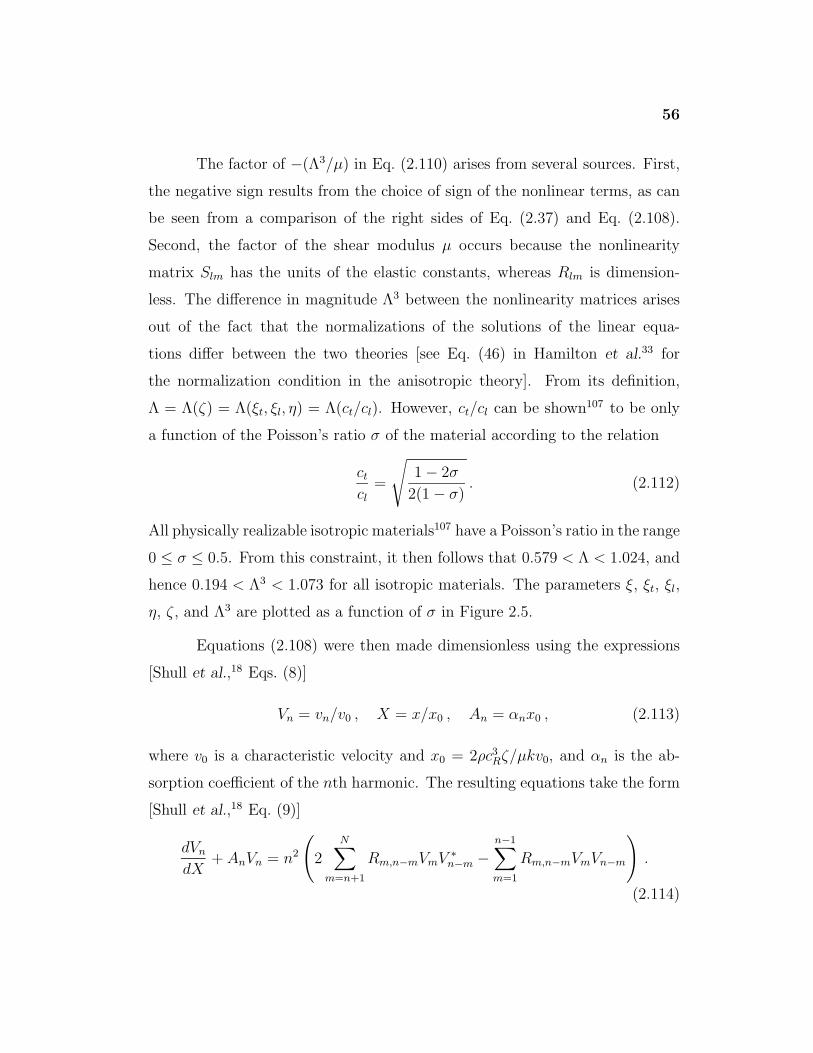
56
The factor of −(Λ3/µ) in Eq. (2.110) arises from several sources. First,
the negative sign results from the choice of sign of the nonlinear terms, as can
be seen from a comparison of the right sides of Eq. (2.37) and Eq. (2.108).
Second, the factor of the shear modulus µ occurs because the nonlinearity
matrix Slm has the units of the elastic constants, whereas Rlm is dimension-
less. The difference in magnitude Λ3 between the nonlinearity matrices arises
out of the fact that the normalizations of the solutions of the linear equa-
tions differ between the two theories [see Eq. (46) in Hamilton et al.33 for
the normalization condition in the anisotropic theory]. From its definition,
Λ = Λ(ζ) = Λ(ξt, ξl, η) = Λ(ct/cl). However, ct/cl can be shown107 to be only
a function of the Poisson’s ratio σ of the material according to the relation
ct
cl
=
√1− 2σ
2(1− σ). (2.112)
All physically realizable isotropic materials107 have a Poisson’s ratio in the range
0 ≤ σ ≤ 0.5. From this constraint, it then follows that 0.579 < Λ < 1.024, and
hence 0.194 < Λ3 < 1.073 for all isotropic materials. The parameters ξ, ξt, ξl,
η, ζ , and Λ3 are plotted as a function of σ in Figure 2.5.
Equations (2.108) were then made dimensionless using the expressions
[Shull et al.,18 Eqs. (8)]
Vn = vn/v0 , X = x/x0 , An = αnx0 , (2.113)
where v0 is a characteristic velocity and x0 = 2ρc3Rζ/µkv0, and αn is the ab-
sorption coefficient of the nth harmonic. The resulting equations take the form
[Shull et al.,18 Eq. (9)]
dVn
dX+ AnVn = n2
(2
N∑m=n+1
Rm,n−mVmV ∗n−m −
n−1∑m=1
Rm,n−mVmVn−m
).
(2.114)
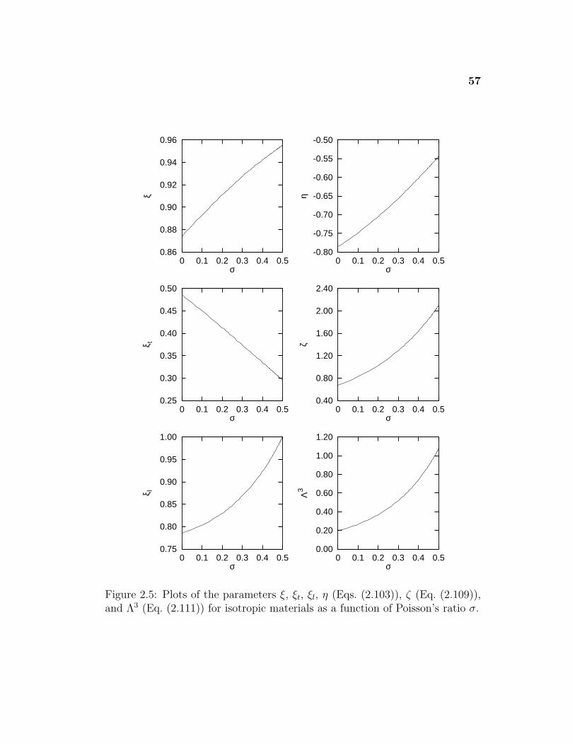
57
0.86
0.88
0.90
0.92
0.94
0.96
0 0.1 0.2 0.3 0.4 0.5
ξ
σ
0.25
0.30
0.35
0.40
0.45
0.50
0 0.1 0.2 0.3 0.4 0.5
ξ t
σ
0.75
0.80
0.85
0.90
0.95
1.00
0 0.1 0.2 0.3 0.4 0.5
ξ l
σ
-0.80
-0.75
-0.70
-0.65
-0.60
-0.55
-0.50
0 0.1 0.2 0.3 0.4 0.5
η
σ
0.40
0.80
1.20
1.60
2.00
2.40
0 0.1 0.2 0.3 0.4 0.5
ζ
σ
0.00
0.20
0.40
0.60
0.80
1.00
1.20
0 0.1 0.2 0.3 0.4 0.5
Λ3
σ
Figure 2.5: Plots of the parameters ξ, ξt, ξl, η (Eqs. (2.103)), ζ (Eq. (2.109)),and Λ3 (Eq. (2.111)) for isotropic materials as a function of Poisson’s ratio σ.
58
These expressions are analogous to Eqs. (82) in Hamilton et al.33 and Eq. (2.40)
here.
2.4.3 Estimates of Nonlinearity Parameters
Shull et al.18 define an estimate for the shock formation distance in an isotropic
solid by
x′ =ρc3
Rζ
4R11µv0k, (2.115)
where ζ , R11, and µ are defined in Section 2.4.2. This expression is obtained
by performing a quasilinear analysis in the same manner as described in Sec-
tion 2.2, and hence the analogue is given by x11 in Eq. (2.59) here. Knight et
al.22 rewrite Eq. (2.115) in the form
x11 = x′ =ρc3
Rζ |ξt + η|4R11µvx0k
, (2.116)
where the characteristic velocity v0 = vx0/|ξt+η| is based upon the longitudinal
velocity amplitude vx0 defined such that vx(0, 0, t) = vx0 sinωt. In this disser-
tation, the corresponding expression is denoted by xx011 and given by Eq. (2.60).
Knight et al. go on to derive a more sophisticated estimate of the shock for-
mation distance [denoted by x+ in Eq. (33) of their paper] based upon an
analysis of the kernel of the time-domain evolution equations for the Rayleigh
wave system. This estimate was also used to model the propagation of SAW
pulses in fused quartz.26 The various expressions discussed in this section are
summarized in Table 2.3.
Knight et al.22 propose a coefficient of nonlinearity for an isotropic solid
of the form [Eq. (29)]
β11 =4µR11
ρc2Rζ |ξt + η| . (2.117)
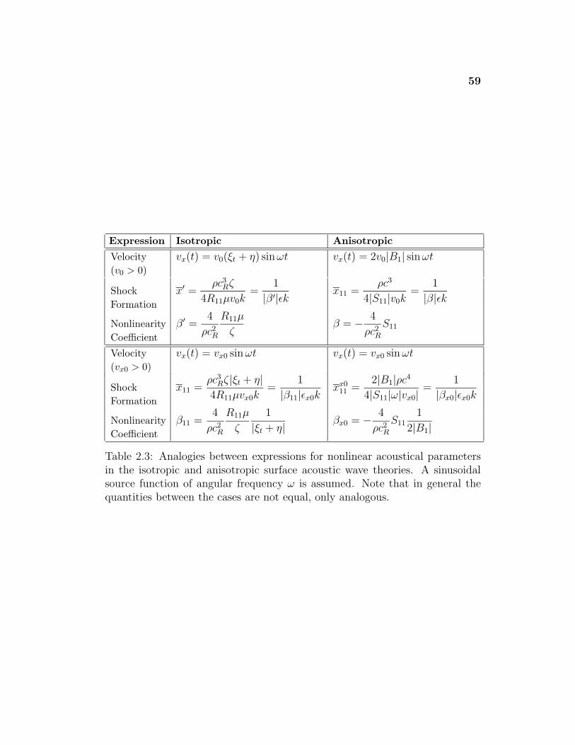
59
Expression Isotropic Anisotropic
Velocity(v0 > 0)
vx(t) = v0(ξt + η) sinωt vx(t) = 2v0|B1| sinωt
ShockFormation
x′ =ρc3
Rζ
4R11µv0k=
1
|β ′|εk x11 =ρc3
4|S11|v0k=
1
|β|εk
NonlinearityCoefficient
β ′ =4
ρc2R
R11µ
ζβ = − 4
ρc2R
S11
Velocity(vx0 > 0)
vx(t) = vx0 sinωt vx(t) = vx0 sin ωt
ShockFormation
x11 =ρc3
Rζ |ξt + η|4R11µvx0k
=1
|β11|εx0kxx0
11 =2|B1|ρc4
4|S11|ω|vx0| =1
|βx0|εx0k
NonlinearityCoefficient
β11 =4
ρc2R
R11µ
ζ
1
|ξt + η| βx0 = − 4
ρc2R
S111
2|B1|
Table 2.3: Analogies between expressions for nonlinear acoustical parametersin the isotropic and anisotropic surface acoustic wave theories. A sinusoidalsource function of angular frequency ω is assumed. Note that in general thequantities between the cases are not equal, only analogous.
60
This coefficient is derived by applying the procedure described in Section 2.2 to
the estimate of the shock formation distance x11 given in Eq. (2.116). Because
x11 of the isotropic theory is analogous to xx0 of the anisotropic theory, β11 is
analogous to the expression for βx0 in Eq. (2.65). Knight et al. go on to derive
a more sophisticated expression for the coefficient of nonlinearity [denoted by
β+ in Eq. (32) of their paper] based on the more sophisticated estimate of
the shock formation distance described in the previous section. The various
expressions discussed in this section are summarized in Table 2.3.
2.4.4 Time-Domain Evolution Equation
In Hamilton et al.,2 it is shown that for nonlinear Rayleigh waves the frequency-
domain evolution equation20
dvn
dx= −n2µω0
2ζρc4R
∑l+m=n
lm
|lm|Rlm (2.118)
has the corresponding time-domain evolution equation for waveforms at the
surface z = 0 given by
∂vx
∂x=
C
c2RT 2
∂
∂τ
∫ T/2
−T/2
∫ T/2
−T/2
L(τ − τ1, τ − τ2)vx(x, τ1)vx(x, τ2) dτ1 dτ2 , (2.119)
where C = −µ/ζρc2R(ξt +η) and ω0 = 2π/T is the angular frequency associated
with a waveform of period T . The kernel of the integral in Eq. (2.119) is given
by
L(τ1, τ2) =∞∑
l=−∞
∞∑m=−∞
|l + m|Rlme−ilω0τ1e−imω0τ2 . (2.120)
The properties of the kernel L were shown to explain the main features of
the harmonic generation and waveform distortion in nonlinear Rayleigh waves.
Equations (2.118), (2.119), and (2.120) are analogous to Eqs. (2.87), (2.94),
and (2.95) in Section 2.3.
61
The relationship between the kernels in the isotropic and anisotropic
cases is determined by comparing Eqs. (2.95) and (2.120). According to Eq.
(2.95), the kernel in the anisotropic case is given by
LS(φBi, τ1, τ2) =
∞∑l=−∞
∞∑m=−∞
Plm(φBi)Qlm(φBi)Slme−ilω0τ1e−imω0τ2 , (2.121)
where
Plm(φ) = i(l + m)eiφ(l+m)/|l+m| , (2.122a)
Qlm(φ) = − lm
|lm|e−iφl/|l|e−iφm/|m| . (2.122b)
For Rayleigh waves, B1 = (ξt + η)i = −|ξt + η|i because ξt + η < 0 for all
isotropic materials (see Figure 2.5 and associated discussion in Section 2.4.2).
Hence |B1| = |ξt + η| and φB1 = −π/2. First, consider Eq. (2.122a) with
n = l + m,
Plm(φ) = ineiφn/|n| =
{i|n|eiφ|n|/|n| for n > 0
−i|n|e−iφ|n|/|n| for n < 0
=
{i|n|eiφ for n > 0
−i|n|e−iφ for n < 0.
(2.123)
With φ = −π/2,
Plm(−π/2) =
{i|n|e−iπ/2 for n < 0
−i|n|eiπ/2 for n > 0
}= |n| . (2.124)
Next, rewrite Eq. (2.122b)
Qlm(φ) = − lm
|lm|e−iφl/|l|e−iφm/|m| . = −
(l
|l|e−iφl/|l|
)(m
|m|e−iφm/|m|
). (2.125)
Observe that
l
|l|e−iφl/|l| =
{ |l||l|e
−iφ|l|/|l| for l > 0−|l||l| eiφ|l|/|l| for l < 0
}=
{e−iφ for l > 0−eiφ for l < 0
. (2.126)
62
Substituting Eq. (2.126) into Eq. (2.125) yields
Qlm(φ) =
−(e−iφ)(e−iφ) for l > 0, m > 0−(e−iφ)(−eiφ) for l > 0, m < 0−(−eiφ)(e−iφ) for l < 0, m > 0−(−eiφ)(−eiφ) for l < 0, m < 0
=
−e−2iφ for l > 0, m > 01 for l > 0, m < 01 for l < 0, m > 0−e2iφ for l < 0, m < 0
.
(2.127)
With φ = −π/2,
Qlm(−π/2) =
−eiπ for l > 0, m > 01 for l > 0, m < 01 for l < 0, m > 0−e−iπ for l < 0, m < 0
= 1 . (2.128)
Substitution of Eq. (2.124) and Eq. (2.128) into Eq. (2.121) yields
LS(−π/2, τ1, τ2) =∞∑
l=−∞
∞∑m=−∞
|l + m|Slme−ilω0τ1e−imω0τ2 . (2.129)
Substitution of Eq. (2.110) into Eq. (2.129) gives
LS(−π/2, τ1, τ2) = − µ
Λ3
∞∑l=−∞
∞∑m=−∞
|l + m|Rlme−ilω0τ1e−imω0τ2 . (2.130)
Equation (2.120) may be substituted into Eq. (2.130) to yield the relation
L(τ1, τ2) = −Λ3
µLS(−π/2, τ1, τ2) . (2.131)
The relationship between the kernels is then the same as that between the
nonlinearity matrices. Note that L(τ1, τ2) implicitly depends on the phase of
the vx velocity component (which was always taken to be φx = −π/2 in previous
work2,18–22,41,100,104).
The relationship between the time-domain evolution equations in the
isotropic and anisotropic cases is determined by comparing Eqs (2.94) and
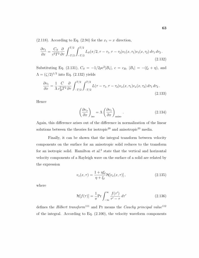
63
(2.118). According to Eq. (2.94) for the x1 = x direction,
∂v1
∂x=
CS
c2T 2
∂
∂τ
∫ T/2
−T/2
∫ T/2
−T/2
LS(π/2, τ − τ1, τ − τ2)v1(x, τ1)v1(x, τ2) dτ1 dτ2 .
(2.132)
Substituting Eq. (2.131), CS = −1/2ρc2|B1|, c = cR, |B1| = −(ξt + η), and
Λ = (ζ/2)1/2 into Eq. (2.132) yields
∂v1
∂x=
1
Λ
C
c2RT 2
∂
∂τ
∫ T/2
−T/2
∫ T/2
−T/2
L(τ − τ1, τ − τ2)vx(x, τ1)vx(x, τ2) dτ1 dτ2 .
(2.133)
Hence (∂vx
∂x
)iso
= Λ
(∂v1
∂x
)aniso
. (2.134)
Again, this difference arises out of the difference in normalization of the linear
solutions between the theories for isotropic20 and anisotropic33 media.
Finally, it can be shown that the integral transform between velocity
components on the surface for an anisotropic solid reduces to the transform
for an isotropic solid. Hamilton et al.2 state that the vertical and horizontal
velocity components of a Rayleigh wave on the surface of a solid are related by
the expression
vz(x, τ) =1 + ηξl
η + ξt
H[vx(x, τ)] , (2.135)
where
H[f(τ)] =1
πPr
∫ ∞
−∞
f(τ ′)τ ′ − τ
dτ ′ (2.136)
defines the Hilbert transform111 and Pr means the Cauchy principal value112
of the integral. According to Eq. (2.100), the velocity waveform components
64
in the x3 and x1 directions (z and x directions) on the surface of a solid are
related by
v3(x, τ) = Re(B3/B1)v1(x, τ)− Im(B3/B1)H[v1(x, τ)] . (2.137)
For an isotropic solid, Eqs. (2.102) imply that
Re
(B3
B1
)= 0 , Im
(B3
B1
)= Im
(1 + ξlη
(ξl + η)i
)= −1 + ξlη
ξl + η, (2.138)
where ξl, η, and ξl are all real-valued (see Figure 2.5). Substituting Eqs. (2.138)
into Eq. (2.137) immediately gives Eq. (2.135) above.
2.5 Summary
This chapter outlined the theory of Hamilton, Il’inskii, and Zabolotskaya33
for the propagation of nonlinear SAWs in anisotropic media. The frequency-
domain model equations which result from this theory are solved in several
quasilinear approximations, and estimates for the shock formation distance and
nonlinearity coefficient are given. A time-domain formulation of the frequency-
domain model equations is derived and shown in the isotropic limit to reduce to
the same time-domain equation for nonlinear Rayleigh waves given by Zabolot-
skaya.20 A detailed comparison is made between the theory for anisotropic
media presented here and the various papers based on the theory of Zabolot-
skaya.20 Many of the quantities defined in Chapter 2 are used extensively
throughout the rest of the dissertation.
Chapter 3
Properties of Cubic Crystals
In order to model the propagation of nonlinear SAWs in a cubic crystal, the
material properties of the crystal must be known. However, the anisotropy of
a crystal adds a significant level of complexity to the problem as compared to
isotropic media. Not only must more information be determined about the bulk
properties of the material, but surface properties such as the orientation of the
surface with respect to the crystalline axes and the direction of propagation
within that surface must be specified as well. This chapter gives a brief overview
of the types of structures, symmetries, and elastic properties found in cubic
crystals. In addition, tables are provided at the end of the chapter listing the
material constants for all the substances investigated in subsequent chapters.
Cubic crystals are chosen for study for several reasons. First, cubic
crystals exhibit the simplest type of fully three-dimensional anisotropy in the
sense that they are the most symmetric. These symmetries are reflected in the
acoustical properties of the crystal and significantly constrain the parameters
that describe these properties.105 Second, investigations of linear bulk acoustic
waves113 and SAWs3 in cubic crystals have shown that the features exhibited by
waves in these materials are similar in many cases to waves in more complicated
crystal types. Finally, many experimental data exist for the elastic constants
of cubic crystals, possibly more than any other type.114,115 It should be noted
that cubic crystals were not chosen because of any limitation imposed by the
theory of Hamilton et al.33 presented in Chapter 2.
65
66
3.1 Crystal Structure
Crystals are generally composed of a periodic array of points (lattice) with one
or more atoms in a specific composition, arrangement, and orientation placed at
each point (basis). The lattice points are typically grouped into parallelepipeds
(unit cells), often with geometrical properties that reflect the symmetries of the
crystal. As the name would suggest, cubic crystals are conventionally described
in terms of unit cells that are cubes, i.e., the edges of the cells are mutually
perpendicular and have equal length. All cubic crystals can be described in
terms of three different lattices (Bravais lattices):
• simple cubic:
Points are placed on each corner of the cube.
• body-centered cubic:
Points are placed on each corner of the cube and in the center of the cube.
• face-centered cubic:
Points are place on each corner of the cube and in the center of each face
of the cube.
Other lattices for crystals with cubic symmetry exist, but all can be constructed
from these lattices. For example, in the diamond cubic structure each atom has
exactly four nearest neighbors. However, this arrangement can be shown to be
two face-centered cubic lattices displaced from one another by a translation of
(1/4, 1/4, 1/4). Reference is made to these various lattice types in the examples
that follow. The directional properties of the crystal are typically given relative
to a standard set of crystalline axes. For cubic crystals, the x, y, and z axes are
conventionally chosen to lie along the three mutually perpendicular directions
of the cubic unit cell.
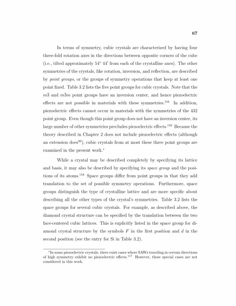
67
In terms of symmetry, cubic crystals are characterized by having four
three-fold rotation axes in the directions between opposite corners of the cube
(i.e., tilted approximately 54◦ 44′ from each of the crystalline axes). The other
symmetries of the crystals, like rotation, inversion, and reflection, are described
by point groups, or the groups of symmetry operations that keep at least one
point fixed. Table 3.2 lists the five point groups for cubic crystals. Note that the
m3 and m3m point groups have an inversion center, and hence piezoelectric
effects are not possible in materials with these symmetries.116 In addition,
piezoelectric effects cannot occur in materials with the symmetries of the 432
point group. Even though this point group does not have an inversion center, its
large number of other symmetries precludes piezoelectric effects.116 Because the
theory described in Chapter 2 does not include piezoelectric effects (although
an extension does50), cubic crystals from at most these three point groups are
examined in the present work.∗
While a crystal may be described completely by specifying its lattice
and basis, it may also be described by specifying its space group and the posi-
tions of its atoms.118 Space groups differ from point groups in that they add
translation to the set of possible symmetry operations. Furthermore, space
groups distinguish the type of crystalline lattice and are more specific about
describing all the other types of the crystal’s symmetries. Table 3.2 lists the
space groups for several cubic crystals. For example, as described above, the
diamond crystal structure can be specified by the translation between the two
face-centered cubic lattices. This is explicitly listed in the space group for di-
amond crystal structure by the symbols F in the first position and d in the
second position (see the entry for Si in Table 3.2).
∗In some piezoelectric crystals, there exist cases where SAWs traveling in certain directionsof high symmetry exhibit no piezoelectric effects.117 However, these special cases are notconsidered in this work.
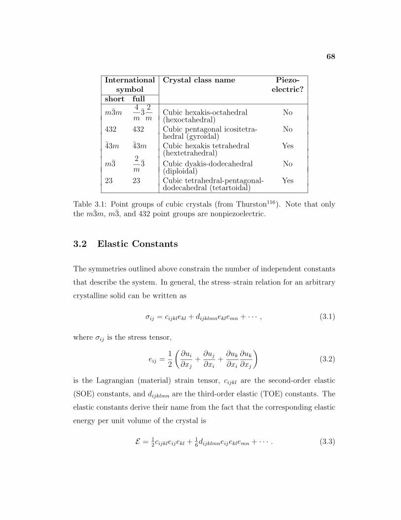
68
International Crystal class name Piezo-symbol electric?
short full
m3m4
m3
2
mCubic hexakis-octahedral No(hexoctahedral)
432 432 Cubic pentagonal icositetra- Nohedral (gyroidal)
43m 43m Cubic hexakis tetrahedral Yes(hextetrahedral)
m32
m3 Cubic dyakis-dodecahedral No
(diploidal)23 23 Cubic tetrahedral-pentagonal- Yes
dodecahedral (tetartoidal)
Table 3.1: Point groups of cubic crystals (from Thurston116). Note that onlythe m3m, m3, and 432 point groups are nonpiezoelectric.
3.2 Elastic Constants
The symmetries outlined above constrain the number of independent constants
that describe the system. In general, the stress–strain relation for an arbitrary
crystalline solid can be written as
σij = cijklekl + dijklmneklemn + · · · , (3.1)
where σij is the stress tensor,
eij =1
2
(∂ui
∂xj+
∂uj
∂xi+
∂uk
∂xi
∂uk
∂xj
)(3.2)
is the Lagrangian (material) strain tensor, cijkl are the second-order elastic
(SOE) constants, and dijklmn are the third-order elastic (TOE) constants. The
elastic constants derive their name from the fact that the corresponding elastic
energy per unit volume of the crystal is
E = 12cijkleijekl + 1
6dijklmneijeklemn + · · · . (3.3)
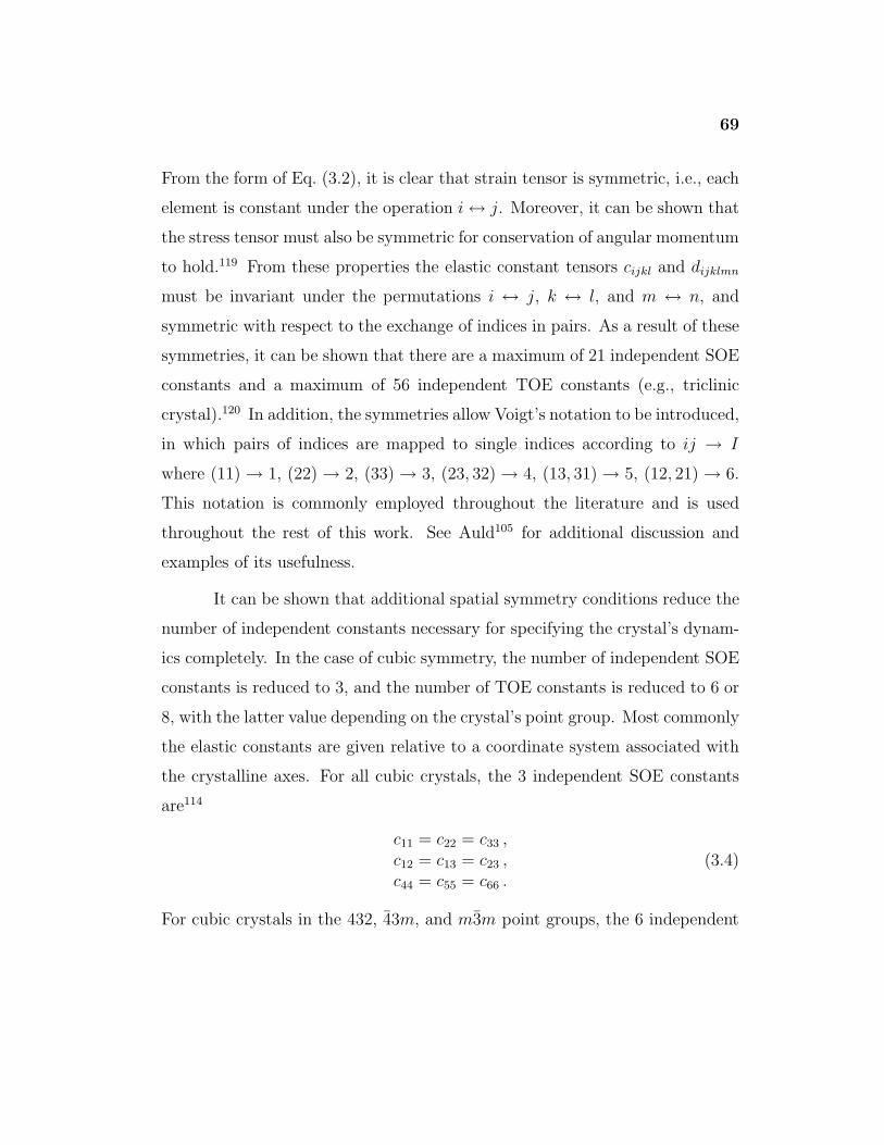
69
From the form of Eq. (3.2), it is clear that strain tensor is symmetric, i.e., each
element is constant under the operation i ↔ j. Moreover, it can be shown that
the stress tensor must also be symmetric for conservation of angular momentum
to hold.119 From these properties the elastic constant tensors cijkl and dijklmn
must be invariant under the permutations i ↔ j, k ↔ l, and m ↔ n, and
symmetric with respect to the exchange of indices in pairs. As a result of these
symmetries, it can be shown that there are a maximum of 21 independent SOE
constants and a maximum of 56 independent TOE constants (e.g., triclinic
crystal).120 In addition, the symmetries allow Voigt’s notation to be introduced,
in which pairs of indices are mapped to single indices according to ij → I
where (11) → 1, (22) → 2, (33) → 3, (23, 32) → 4, (13, 31) → 5, (12, 21) → 6.
This notation is commonly employed throughout the literature and is used
throughout the rest of this work. See Auld105 for additional discussion and
examples of its usefulness.
It can be shown that additional spatial symmetry conditions reduce the
number of independent constants necessary for specifying the crystal’s dynam-
ics completely. In the case of cubic symmetry, the number of independent SOE
constants is reduced to 3, and the number of TOE constants is reduced to 6 or
8, with the latter value depending on the crystal’s point group. Most commonly
the elastic constants are given relative to a coordinate system associated with
the crystalline axes. For all cubic crystals, the 3 independent SOE constants
are114
c11 = c22 = c33 ,c12 = c13 = c23 ,c44 = c55 = c66 .
(3.4)
For cubic crystals in the 432, 43m, and m3m point groups, the 6 independent
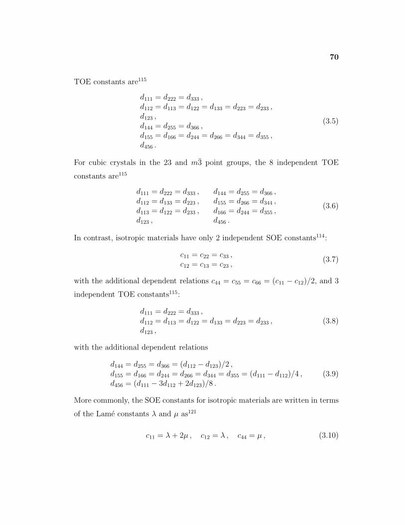
70
TOE constants are115
d111 = d222 = d333 ,d112 = d113 = d122 = d133 = d223 = d233 ,d123 ,d144 = d255 = d366 ,d155 = d166 = d244 = d266 = d344 = d355 ,d456 .
(3.5)
For cubic crystals in the 23 and m3 point groups, the 8 independent TOE
constants are115
d111 = d222 = d333 , d144 = d255 = d366 ,d112 = d133 = d223 , d155 = d266 = d344 ,d113 = d122 = d233 , d166 = d244 = d355 ,d123 , d456 .
(3.6)
In contrast, isotropic materials have only 2 independent SOE constants114:
c11 = c22 = c33 ,c12 = c13 = c23 ,
(3.7)
with the additional dependent relations c44 = c55 = c66 = (c11 − c12)/2, and 3
independent TOE constants115:
d111 = d222 = d333 ,d112 = d113 = d122 = d133 = d223 = d233 ,d123 ,
(3.8)
with the additional dependent relations
d144 = d255 = d366 = (d112 − d123)/2 ,d155 = d166 = d244 = d266 = d344 = d355 = (d111 − d112)/4 ,d456 = (d111 − 3d112 + 2d123)/8 .
(3.9)
More commonly, the SOE constants for isotropic materials are written in terms
of the Lame constants λ and µ as121
c11 = λ + 2µ , c12 = λ , c44 = µ , (3.10)
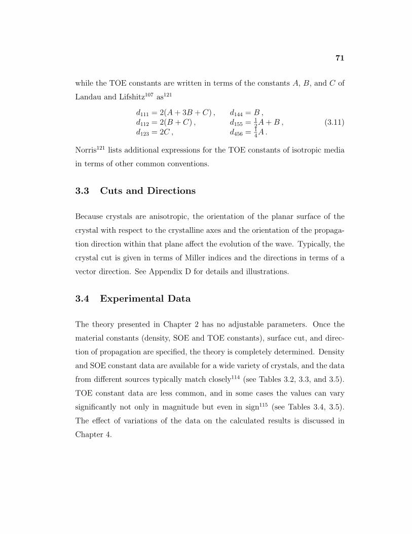
71
while the TOE constants are written in terms of the constants A, B, and C of
Landau and Lifshitz107 as121
d111 = 2(A + 3B + C) , d144 = B ,d112 = 2(B + C) , d155 = 1
2A + B ,
d123 = 2C , d456 = 14A .
(3.11)
Norris121 lists additional expressions for the TOE constants of isotropic media
in terms of other common conventions.
3.3 Cuts and Directions
Because crystals are anisotropic, the orientation of the planar surface of the
crystal with respect to the crystalline axes and the orientation of the propaga-
tion direction within that plane affect the evolution of the wave. Typically, the
crystal cut is given in terms of Miller indices and the directions in terms of a
vector direction. See Appendix D for details and illustrations.
3.4 Experimental Data
The theory presented in Chapter 2 has no adjustable parameters. Once the
material constants (density, SOE and TOE constants), surface cut, and direc-
tion of propagation are specified, the theory is completely determined. Density
and SOE constant data are available for a wide variety of crystals, and the data
from different sources typically match closely114 (see Tables 3.2, 3.3, and 3.5).
TOE constant data are less common, and in some cases the values can vary
significantly not only in magnitude but even in sign115 (see Tables 3.4, 3.5).
The effect of variations of the data on the calculated results is discussed in
Chapter 4.
72
3.5 Summary
This chapter has discussed some of the basic properties of cubic crystals in-
cluding structure, symmetries, and elastic constants. Of the five point groups
that fall into the cubic class, only three (m3m, 432, and m3) have symmetries
which exclude piezoelectric effects. All three groups have three independent
SOE constants. In contrast, the m3m and 432 point groups have six indepen-
dent TOE constants, while the m3 point group has eight independent TOE
constants. For reference purposes, measured densities, SOE constants, and
TOE elastic constants from the literature are listed in Tables 3.2, 3.3, 3.4, and
3.5 for crystals in the m3m and m3 point groups. Chapters 4, 5, and 6 use the
information contained in this chapter to investigate nonlinear SAWs propagat-
ing in crystals of the m3m and m3 point groups over a variety surface cuts and
directions.
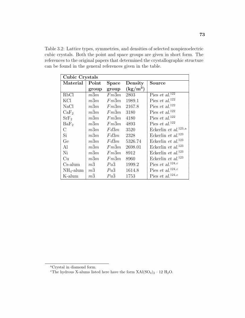
73
Table 3.2: Lattice types, symmetries, and densities of selected nonpiezoelectriccubic crystals. Both the point and space groups are given in short form. Thereferences to the original papers that determined the crystallographic structurecan be found in the general references given in the table.
Cubic CrystalsMaterial Point Space Density Source
group group (kg/m3)RbCl m3m Fm3m 2803 Pies et al.122
KCl m3m Fm3m 1989.1 Pies et al.122
NaCl m3m Fm3m 2167.8 Pies et al.122
CaF2 m3m Fm3m 3180 Pies et al.122
SrF2 m3m Fm3m 4180 Pies et al.122
BaF2 m3m Fm3m 4893 Pies et al.122
C m3m Fd3m 3520 Eckerlin et al.123,a
Si m3m Fd3m 2328 Eckerlin et al.123
Ge m3m Fd3m 5326.74 Eckerlin et al.123
Al m3m Fm3m 2698.01 Eckerlin et al.123
Ni m3m Fm3m 8912 Eckerlin et al.123
Cu m3m Fm3m 8960 Eckerlin et al.123
Cs-alum m3 Pa3 1999.2 Pies et al.124,c
NH4-alum m3 Pa3 1614.8 Pies et al.124,c
K-alum m3 Pa3 1753 Pies et al.124,c
aCrystal in diamond form.cThe hydrous X-alums listed here have the form XAl(SO4)2 · 12 H2O.
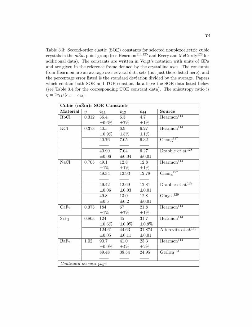
74
Table 3.3: Second-order elastic (SOE) constants for selected nonpiezoelectric cubiccrystals in the m3m point group (see Hearmon114,125 and Every and McCurdy126 foradditional data). The constants are written in Voigt’s notation with units of GPaand are given in the reference frame defined by the crystalline axes. The constantsfrom Hearmon are an average over several data sets (not just those listed here), andthe percentage error listed is the standard deviation divided by the average. Paperswhich contain both SOE and TOE constant data have the SOE data listed below(see Table 3.4 for the corresponding TOE constant data). The anisotropy ratio isη = 2c44/(c11 − c12).
Cubic (m3m): SOE ConstantsMaterial η c11 c12 c44 SourceRbCl 0.312 36.4 6.3 4.7 Hearmon114
±0.6% ±7% ±1%KCl 0.373 40.5 6.9 6.27 Hearmon114
±0.9% ±5% ±1%40.76 7.05 6.32 Chang127
40.90 7.04 6.27 Drabble et al.128
±0.06 ±0.04 ±0.01NaCl 0.705 49.1 12.8 12.8 Hearmon114
±1% ±1% ±1%49.34 12.93 12.78 Chang127
49.42 12.69 12.81 Drabble et al.128
±0.06 ±0.03 ±0.0149.8 13.0 12.8 Gluyas129
±0.5 ±0.2 ±0.01CaF2 0.373 184 67 21.8 Hearmon114
±1% ±7% ±1%SrF2 0.803 124 45 31.7 Hearmon114
±0.6% ±0.9% ±0.9%124.61 44.63 31.874 Alterovitz et al.130
±0.05 ±0.11 ±0.01BaF2 1.02 90.7 41.0 25.3 Hearmon114
±0.9% ±4% ±2%89.48 38.54 24.95 Gerlich131
Continued on next page
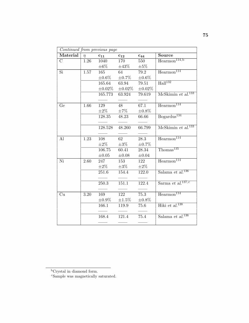
75
Continued from previous pageMaterial η c11 c12 c44 SourceC 1.26 1040 170 550 Hearmon114,b
±6% ±43% ±5%Si 1.57 165 64 79.2 Hearmon114
±0.6% ±0.7% ±0.6%165.64 63.94 79.51 Hall132
±0.02% ±0.02% ±0.02%165.773 63.924 79.619 McSkimin et al.133
Ge 1.66 129 48 67.1 Hearmon114
±2% ±7% ±0.8%128.35 48.23 66.66 Bogardus134
128.528 48.260 66.799 McSkimin et al.133
Al 1.23 108 62 28.3 Hearmon114
±2% ±3% ±0.7%106.75 60.41 28.34 Thomas135
±0.05 ±0.08 ±0.04Ni 2.60 247 153 122 Hearmon114
±2% ±3% ±2%251.6 154.4 122.0 Salama et al.136
250.3 151.1 122.4 Sarma et al.137,c
Cu 3.20 169 122 75.3 Hearmon114
±0.9% ±1.5% ±0.8%166.1 119.9 75.6 Hiki et al.138
168.4 121.4 75.4 Salama et al.136
bCrystal in diamond form.cSample was magnetically saturated.
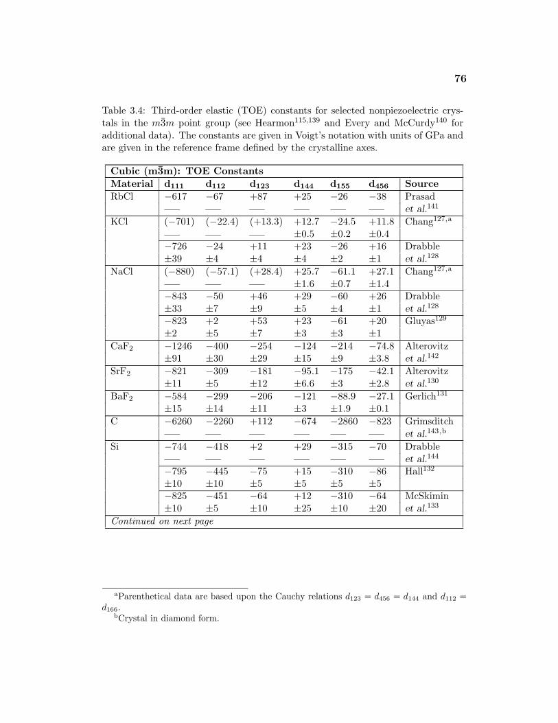
76
Table 3.4: Third-order elastic (TOE) constants for selected nonpiezoelectric crys-tals in the m3m point group (see Hearmon115,139 and Every and McCurdy140 foradditional data). The constants are given in Voigt’s notation with units of GPa andare given in the reference frame defined by the crystalline axes.
Cubic (m3m): TOE ConstantsMaterial d111 d112 d123 d144 d155 d456 SourceRbCl −617 −67 +87 +25 −26 −38 Prasad
et al.141
KCl (−701) (−22.4) (+13.3) +12.7 −24.5 +11.8 Chang127,a
±0.5 ±0.2 ±0.4−726 −24 +11 +23 −26 +16 Drabble±39 ±4 ±4 ±4 ±2 ±1 et al.128
NaCl (−880) (−57.1) (+28.4) +25.7 −61.1 +27.1 Chang127,a
±1.6 ±0.7 ±1.4−843 −50 +46 +29 −60 +26 Drabble±33 ±7 ±9 ±5 ±4 ±1 et al.128
−823 +2 +53 +23 −61 +20 Gluyas129
±2 ±5 ±7 ±3 ±3 ±1CaF2 −1246 −400 −254 −124 −214 −74.8 Alterovitz
±91 ±30 ±29 ±15 ±9 ±3.8 et al.142
SrF2 −821 −309 −181 −95.1 −175 −42.1 Alterovitz±11 ±5 ±12 ±6.6 ±3 ±2.8 et al.130
BaF2 −584 −299 −206 −121 −88.9 −27.1 Gerlich131
±15 ±14 ±11 ±3 ±1.9 ±0.1C −6260 −2260 +112 −674 −2860 −823 Grimsditch
et al.143,b
Si −744 −418 +2 +29 −315 −70 Drabbleet al.144
−795 −445 −75 +15 −310 −86 Hall132
±10 ±10 ±5 ±5 ±5 ±5−825 −451 −64 +12 −310 −64 McSkimin±10 ±5 ±10 ±25 ±10 ±20 et al.133
Continued on next page
aParenthetical data are based upon the Cauchy relations d123 = d456 = d144 and d112 =d166.
bCrystal in diamond form.
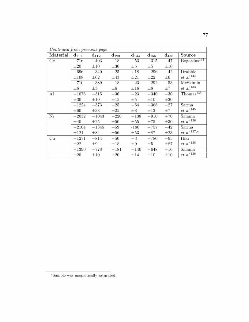
77
Continued from previous pageMaterial d111 d112 d123 d144 d155 d456 SourceGe −716 −403 −18 −53 −315 −47 Bogardus134
±20 ±10 ±30 ±5 ±5 ±10−696 −340 +25 +18 −296 −42 Drabble±108 ±62 ±43 ±21 ±22 ±6 et al.144
−710 −389 −18 −23 −292 −53 McSkimin±6 ±3 ±6 ±16 ±8 ±7 et al.133
Al −1076 −315 +36 −23 −340 −30 Thomas135
±30 ±10 ±15 ±5 ±10 ±30−1224 −373 +25 −64 −368 −27 Sarma±60 ±38 ±25 ±8 ±13 ±7 et al.145
Ni −2032 −1043 −220 −138 −910 +70 Salama±40 ±25 ±50 ±55 ±75 ±30 et al.136
−2104 −1345 +59 -180 −757 −42 Sarma±124 ±84 ±56 ±53 ±87 ±23 et al.137,c
Cu −1271 −814 −50 −3 −780 −95 Hiki±22 ±9 ±18 ±9 ±5 ±87 et al.138
−1390 −778 −181 −140 −648 −16 Salama±20 ±10 ±20 ±14 ±10 ±10 et al.136
cSample was magnetically saturated.
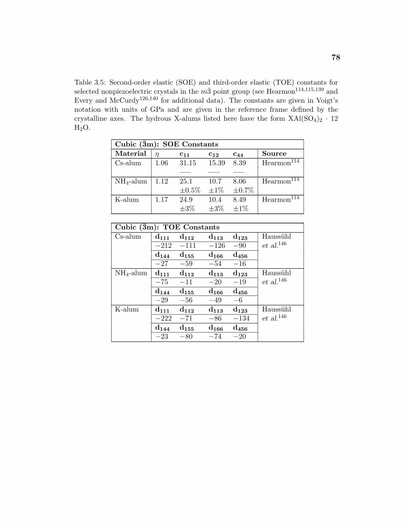
78
Table 3.5: Second-order elastic (SOE) and third-order elastic (TOE) constants forselected nonpiezoelectric crystals in the m3 point group (see Hearmon114,115,139 andEvery and McCurdy126,140 for additional data). The constants are given in Voigt’snotation with units of GPa and are given in the reference frame defined by thecrystalline axes. The hydrous X-alums listed here have the form XAl(SO4)2 · 12H2O.
Cubic (3m): SOE ConstantsMaterial η c11 c12 c44 SourceCs-alum 1.06 31.15 15.39 8.39 Hearmon114
NH4-alum 1.12 25.1 10.7 8.06 Hearmon114
±0.5% ±1% ±0.7%K-alum 1.17 24.9 10.4 8.49 Hearmon114
±3% ±3% ±1%
Cubic (3m): TOE ConstantsCs-alum d111 d112 d113 d123 Haussuhl
−212 −111 −126 −90 et al.146
d144 d155 d166 d456
−27 −59 −54 −16NH4-alum d111 d112 d113 d123 Haussuhl
−75 −11 −20 −19 et al.146
d144 d155 d166 d456
−29 −56 −49 −6K-alum d111 d112 d113 d123 Haussuhl
−222 −71 −86 −134 et al.146
d144 d155 d166 d456
−23 −80 −74 −20
Chapter 4
Monofrequency SAWs in the (001) Plane
Consider the case where the crystal surface is the (001) plane, or equivalently,
the xy plane of crystalline axes. (See Figure D.1 for a diagram of this cut.) This
chapter examines the properties of surface acoustic waves in this plane for a
variety of crystals. To begin, some of the basic linear properties of surface waves
in the (001) cut are briefly reviewed. Attention is focused next on the nonlinear
properties, first on the general properties of a variety of materials, and then
on a few materials which show characteristic behaviors. To show the basic
features of the nonlinear processes most clearly, only monofrequency source
conditions are considered. Numerical simulations based on the theory presented
in Chapter 2 are used to compare and contrast the harmonic generation and
waveform distortion between the various cases considered.
4.1 Linear Effects
As mentioned in Chapter 2, crystalline anisotropy manifests itself in SAWs
even in the linear regime. The primary consequences are that (1) the wave
speed is a function of propagation direction and (2) the direction of power flow
is no longer necessarily coincident with the direction of propagation. The latter
effect is also a function of propagation direction.
The properties of linear SAWs are expounded at length in the review
by Farnell.3 Hence the discussion here is brief and discusses only the materials
that are examined later for nonlinear effects.
79
80
Farnell showed that the qualitative and quantitative variation of the
linear wave speed as a function of angle may be characterized by the anisotropy
ratio
η =2c66
c11 − c12. (4.1)
This definition is constructed such that η = 1 for an isotropic material (it is
also sometimes written with c44 instead of c66 for cubic crystals because these
constants are equivalent under cubic symmetry). Farnell also showed that
the SAW speeds for many materials conveniently group by anisotropy ratio.
Qualitatively, a higher anisotropy ratio implies a slower SAW speed relative
to the fast transverse bulk wave speed. Because of this grouping, he was able
to focus on selected materials as characteristic of many others. He chose to
highlight Ni as a characteristic material with η > 1 and KCl as a characteristic
material with η < 1. Table 4.1 lists the anisotropy ratio of many materials,
all of which also have experimentally determined TOE constants. This latter
property makes them candidates for study in the nonlinear regime.
Royer and Dieulesaint117 looked for SAW solutions in orthorhombic,
tetragonal, hexagonal, and cubic crystals under the condition that the dis-
placement of the SAW is confined to the sagittal plane. In these cases, an
analytical solution is possible (similar to the way such a solution is possible
for the propagation of Rayleigh waves in isotropic media). For cubic crystals,
Royer and Dieulesaint show that solutions with sagittal plane polarization exist
in the cases:
1. 〈100〉 direction of the (001) plane and the other cuts and directions that
are equivalent by symmetry [e.g., the 〈010〉 direction of (001) plane, the
〈010〉 direction of the (100) plane],
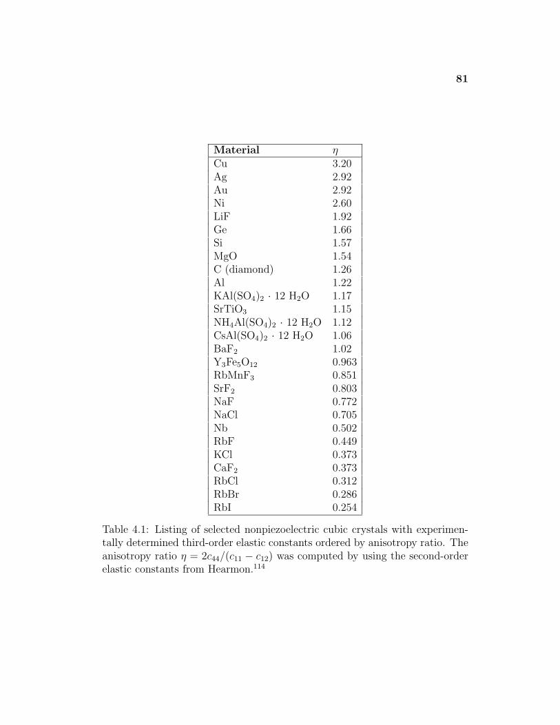
81
Material ηCu 3.20Ag 2.92Au 2.92Ni 2.60LiF 1.92Ge 1.66Si 1.57MgO 1.54C (diamond) 1.26Al 1.22KAl(SO4)2 · 12 H2O 1.17SrTiO3 1.15NH4Al(SO4)2 · 12 H2O 1.12CsAl(SO4)2 · 12 H2O 1.06BaF2 1.02Y3Fe5O12 0.963RbMnF3 0.851SrF2 0.803NaF 0.772NaCl 0.705Nb 0.502RbF 0.449KCl 0.373CaF2 0.373RbCl 0.312RbBr 0.286RbI 0.254
Table 4.1: Listing of selected nonpiezoelectric cubic crystals with experimen-tally determined third-order elastic constants ordered by anisotropy ratio. Theanisotropy ratio η = 2c44/(c11 − c12) was computed by using the second-orderelastic constants from Hearmon.114
82
2. 〈110〉 direction of the (001) plane and the other cuts and directions that
are equivalent by symmetry [e.g., the 〈110〉 and 〈110〉 directions of the
(001) plane],
3. 〈110〉 direction of the (110) plane and the other cuts and directions that
are equivalent by symmetry [e.g., the 〈110〉 direction of the (110) plane],
4. 〈001〉 direction of the (110) plane and the other cuts and directions that
are equivalent by symmetry [e.g., the 〈001〉 direction of the (110) plane],
While these solutions are only a small subset of all the generalized Rayleigh
wave solutions for a given crystal, their relative simplicity allowed them to be
the first solutions studied for SAWs in crystals.∗
Royer and Dieulesaint also discussed the influence of the anisotropy
ratio η on the solutions with sagittal plane polarization in cubic and tetragonal
systems. They showed that for propagation directions where the magnitudes
of the displacement components decay as an exponentially damped sinusoid,
ui(x, z, t) = f(x, t)e−hkz cos(gkz + φ) , (4.2)
then the SAW speed c relative to the transverse bulk wave speed ct =√
c66/ρ
can be approximated by
c
ct
≈[2
η
(1− c66
c11
1
η
)]1/2
, η � 1 , (4.3)
and the decay coefficient can be written as
h ≈ (1 + c66/c11)/2η , η � 1 . (4.4)
∗Stoneley published studies of SAW propagation in the basal plane of hexagonal crys-tals147 (the plane normal to the sixfold symmetry axis) in 1949 and the 〈100〉 and 〈110〉directions in the (001) plane of cubic crystals148 in 1955.
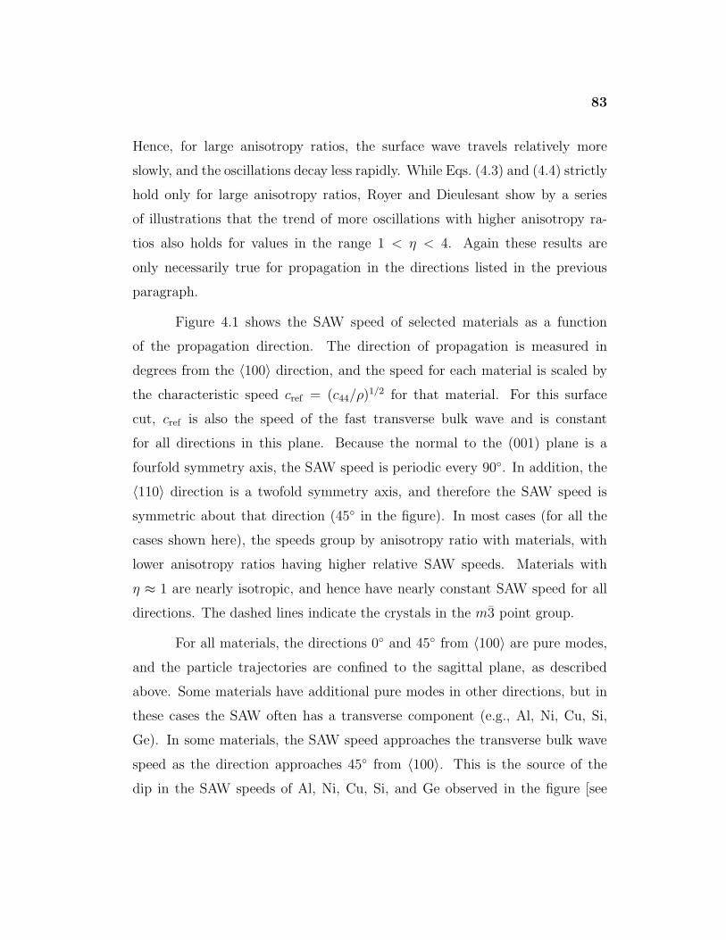
83
Hence, for large anisotropy ratios, the surface wave travels relatively more
slowly, and the oscillations decay less rapidly. While Eqs. (4.3) and (4.4) strictly
hold only for large anisotropy ratios, Royer and Dieulesant show by a series
of illustrations that the trend of more oscillations with higher anisotropy ra-
tios also holds for values in the range 1 < η < 4. Again these results are
only necessarily true for propagation in the directions listed in the previous
paragraph.
Figure 4.1 shows the SAW speed of selected materials as a function
of the propagation direction. The direction of propagation is measured in
degrees from the 〈100〉 direction, and the speed for each material is scaled by
the characteristic speed cref = (c44/ρ)1/2 for that material. For this surface
cut, cref is also the speed of the fast transverse bulk wave and is constant
for all directions in this plane. Because the normal to the (001) plane is a
fourfold symmetry axis, the SAW speed is periodic every 90◦. In addition, the
〈110〉 direction is a twofold symmetry axis, and therefore the SAW speed is
symmetric about that direction (45◦ in the figure). In most cases (for all the
cases shown here), the speeds group by anisotropy ratio with materials, with
lower anisotropy ratios having higher relative SAW speeds. Materials with
η ≈ 1 are nearly isotropic, and hence have nearly constant SAW speed for all
directions. The dashed lines indicate the crystals in the m3 point group.
For all materials, the directions 0◦ and 45◦ from 〈100〉 are pure modes,
and the particle trajectories are confined to the sagittal plane, as described
above. Some materials have additional pure modes in other directions, but in
these cases the SAW often has a transverse component (e.g., Al, Ni, Cu, Si,
Ge). In some materials, the SAW speed approaches the transverse bulk wave
speed as the direction approaches 45◦ from 〈100〉. This is the source of the
dip in the SAW speeds of Al, Ni, Cu, Si, and Ge observed in the figure [see
84
0.6
0.7
0.8
0.9
1.0
0 10 20 30 40 50 60 70 80 90
Rel
ativ
e V
eloc
ity
Angle from ⟨100⟩ [degrees]
Relative Velocity vs. Angle in (001) planeη=0.312RbCl
CaF2 η=0.373η=0.373KCl
NaCl η=0.705SrF 2 η=0.803
η=1.02η=1.06Cs-alum
-alum4 η=1.12NHK-alum η=1.17
Al η=1.22
C η=1.26
Si η=1.57
Ge η=1.66
Ni η=2.60
Cu η=3.20
BaF2
Figure 4.1: Dependence of SAW speed on direction of propagation in the (001)plane for selected materials. The SAW speed of each material is measuredrelative to cref = (c44/ρ)1/2 and is periodic every 90◦. The dashed lines indicatecrystals in the m3 point group.
85
also Figures 4.3(d) and 4.14(d)]. The SAW then becomes an exceptional bulk
wave in the 45◦ direction. This degeneracy then gives rise to a pseudosurface
wave mode in that same direction (see Appendix B for more discussion of these
phenomena).
All of these are linear effects; they are mentioned here to set a context
for nonlinear effects to be discussed next.
4.2 Nonlinear Effects
This section shows that:
• Plots of the first few nonlinearity matrix elements as a function of direc-
tion can provide a map of the kind of waveform distortion that occurs
in various directions in the surface. This observation is advantageous
because it allows the waveform evolution to be characterized without re-
quiring the numerical integration of any nonlinear differential equations.
• The nonlinearity matrix elements sometimes change in magnitude and
sign as a function of direction. These changes are often proportionally
larger than variations of linear quantities over the same range. In exper-
imental situations where it is difficult to excite waves of large amplitude,
the nonlinear effects may be weak. In these cases large changes in non-
linearity parameters may be easier to measure than small ones.
• Directions may exist where no shock formation occurs even for finite
amplitude waves. This phenomenon arises from weak coupling between
certain harmonics, which prevents the transfer of energy to higher har-
monics necessary for shock formation.
86
• Directions exist where the energy transfer to higher harmonics occurs
more rapidly and shock formation is enhanced.
To some extent, the topics examined here parallel the review by Farnell3 and
provide the nonlinear extension to some of the cases considered there. As is
shown below, cubic crystals exhibit wide diversity in their nonlinear properties.
Fifteen crystals were chosen for study based on their crystalline symmetries
and structure. However, for purposes of simplicity, detailed studies have been
performed only on a smaller set of representative materials. In particular, Si is
studied most intensively due to its practical importance. Attention is also given
to Ni and KCl because these materials were chosen as characteristic examples
by Farnell. It proves useful to define the dimensionless nonlinearity matrix
Slm = −Slm
c44. (4.5)
The negative sign is introduced to be consistent in sign with the nonlinearity
matrix elements Rlm used for nonlinear Rayleigh waves.18 In all cases, the
figures in the remaining chapters use matrix elements defined by Eq. (4.5).
4.2.1 General Study
Figure 4.2 shows plots of the nonlinearity matrix elements for a variety of
crystals. Each graph plots S11 (solid), S12 (long dashed), and S13 (short dashed)
over the range of directions 0◦ to 45◦ from 〈100〉, where the elastic constant
c44 is the corresponding constant for each material type. The vertical scale on
each plot is adjusted to show the curves most clearly for each material. While
plotting only three elements of the nonlinearity matrix certainly does not give
a full description of the nonlinear properties of the SAW, it can give a good
idea of the evolution in many cases, as is shown below.
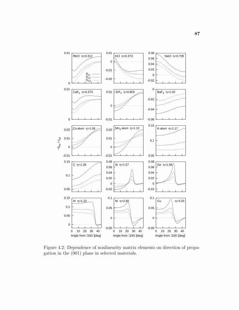
87
0
0.01
RbCl η=0.312
S11S12S13
-0.02
-0.01
0
0.01
KCl η=0.373
-0.02
0
0.02
0.04
0.06
0.08
NaCl η=0.705
0
0.01
CaF2 η=0.373
-0.01
0
0.01
SrF2 η=0.803
-0.06
-0.04
-0.02
0
BaF2 η=1.02
0
0.05
0.1
0.15
0 10 20 30 40
Al η=1.22
Angle from ⟨100⟩ [deg]
-0.05
0
0.05
0.1
0 10 20 30 40
Ni η=2.60
Angle from ⟨100⟩ [deg]
-0.05
0
0.05
0.1
0 10 20 30 40
Cu η=3.20
Angle from ⟨100⟩ [deg]
0.05
0.1
0.15
C η=1.26
-0.02
0
0.02
0.04
0.06
0.08
Si η=1.57
-0.02
0
0.02
0.04
0.06
0.08
Ge η=1.66
-0.01
0
0.01
0.02
Cs-alum η=1.06
-0.01
0
0.01
0.02
NH4-alum η=1.12
0.05
0.1
0.15
K-alum η=1.17
−Slm
/ c 4
4
Normalized Nonlinearity Matrix Elements in (001) Plane for Selected Materials
Figure 4.2: Dependence of nonlinearity matrix elements on direction of propa-gation in the (001) plane in selected materials.
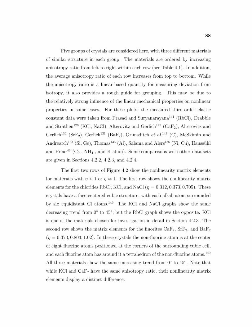
88
Five groups of crystals are considered here, with three different materials
of similar structure in each group. The materials are ordered by increasing
anisotropy ratio from left to right within each row (see Table 4.1). In addition,
the average anisotropy ratio of each row increases from top to bottom. While
the anisotropy ratio is a linear-based quantity for measuring deviation from
isotropy, it also provides a rough guide for grouping. This may be due to
the relatively strong influence of the linear mechanical properties on nonlinear
properties in some cases. For these plots, the measured third-order elastic
constant data were taken from Prasad and Suryanarayana141 (RbCl), Drabble
and Strathen128 (KCl, NaCl), Alterovitz and Gerlich142 (CaF2), Alterovitz and
Gerlich130 (SrF2), Gerlich131 (BaF2), Grimsditch et al.143 (C), McSkimin and
Andreatch133 (Si, Ge), Thomas135 (Al), Salama and Alers136 (Ni, Cu), Haussuhl
and Preu146 (Cs-, NH4-, and K-alum). Some comparisons with other data sets
are given in Sections 4.2.2, 4.2.3, and 4.2.4.
The first two rows of Figure 4.2 show the nonlinearity matrix elements
for materials with η < 1 or η ≈ 1. The first row shows the nonlinearity matrix
elements for the chlorides RbCl, KCl, and NaCl (η = 0.312, 0.373, 0.705). These
crystals have a face-centered cubic structure, with each alkali atom surrounded
by six equidistant Cl atoms.149 The KCl and NaCl graphs show the same
decreasing trend from 0◦ to 45◦, but the RbCl graph shows the opposite. KCl
is one of the materials chosen for investigation in detail in Section 4.2.3. The
second row shows the matrix elements for the fluorites CaF2, SrF2, and BaF2
(η = 0.373, 0.803, 1.02). In these crystals the non-fluorine atom is at the center
of eight fluorine atoms positioned at the corners of the surrounding cubic cell,
and each fluorine atom has around it a tetrahedron of the non-fluorine atoms.149
All three materials show the same increasing trend from 0◦ to 45◦. Note that
while KCl and CaF2 have the same anisotropy ratio, their nonlinearity matrix
elements display a distinct difference.
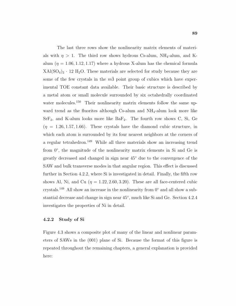
89
The last three rows show the nonlinearity matrix elements of materi-
als with η > 1. The third row shows hydrous Cs-alum, NH4-alum, and K-
alum (η = 1.06, 1.12, 1.17) where a hydrous X-alum has the chemical formula
XAl(SO4)2 · 12 H2O. These materials are selected for study because they are
some of the few crystals in the m3 point group of cubics which have exper-
imental TOE constant data available. Their basic structure is described by
a metal atom or small molecule surrounded by six octahedrally coordinated
water molecules.150 Their nonlinearity matrix elements follow the same up-
ward trend as the fluorites although Cs-alum and NH4-alum look more like
SrF2, and K-alum looks more like BaF2. The fourth row shows C, Si, Ge
(η = 1.26, 1.57, 1.66). These crystals have the diamond cubic structure, in
which each atom is surrounded by its four nearest neighbors at the corners of
a regular tetrahedron.149 While all three materials show an increasing trend
from 0◦, the magnitude of the nonlinearity matrix elements in Si and Ge is
greatly decreased and changed in sign near 45◦ due to the convergence of the
SAW and bulk transverse modes in that angular region. This effect is discussed
further in Section 4.2.2, where Si is investigated in detail. Finally, the fifth row
shows Al, Ni, and Cu (η = 1.22, 2.60, 3.20). These are all face-centered cubic
crystals.149 All show an increase in the nonlinearity from 0◦ and all show a sub-
stantial decrease and change in sign near 45◦, much like Si and Ge. Section 4.2.4
investigates the properties of Ni in detail.
4.2.2 Study of Si
Figure 4.3 shows a composite plot of many of the linear and nonlinear param-
eters of SAWs in the (001) plane of Si. Because the format of this figure is
repeated throughout the remaining chapters, a general explanation is provided
here:
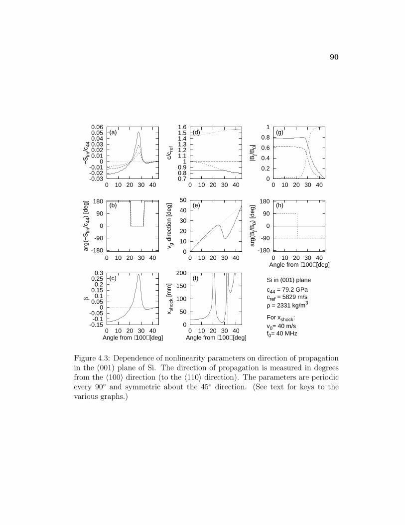
90
-0.03-0.02-0.01
0 0.01 0.02 0.03 0.04 0.05 0.06
0 10 20 30 40
−Slm
/c44
(a)
-180
-90
0
90
180
0 10 20 30 40
arg(
−Slm
/c44
) [d
eg]
(b)
-0.15 -0.1
-0.05 0
0.05 0.1
0.15 0.2
0.25 0.3
0 10 20 30 40
β
(c)
Angle from ⟨100⟩ [deg]
0.7 0.8 0.9 1
1.1 1.2 1.3 1.4 1.5 1.6
0 10 20 30 40
c/c r
ef
(d)
0
10
20
30
40
50
0 10 20 30 40
v g d
irect
ion
[deg
] (e)
0
50
100
150
200
0 10 20 30 40
x sho
ck [m
m]
(f)
Angle from ⟨100⟩ [deg]
0
0.2
0.4
0.6
0.8
1
0 10 20 30 40
|Bj/B
0|
(g)
-180
-90
0
90
180
0 10 20 30 40ar
g(B
j/B0)
[deg
] (h)
Angle from ⟨100⟩ [deg]
Si in (001) plane
c44 = 79.2 GPacref = 5829 m/sρ = 2331 kg/m3
For xshock:v0= 40 m/sf0= 40 MHz
Figure 4.3: Dependence of nonlinearity parameters on direction of propagationin the (001) plane of Si. The direction of propagation is measured in degreesfrom the 〈100〉 direction (to the 〈110〉 direction). The parameters are periodicevery 90◦ and symmetric about the 45◦ direction. (See text for keys to thevarious graphs.)
91
• Figure 4.3(a) shows the nonlinearity matrix elements [recall Eq. (4.5)]
S11 (solid), S12 (long dashed), and S13 (short dashed) as a function of
direction. In the (001) plane, the nonlinearity matrix elements are purely
real-valued, symmetric about the direction 45◦ from 〈100〉, and periodic
every 90◦. As in Figure 4.2, the matrix elements are scaled by the SOE
constant c44 (given in the lower right corner of the figure).
• Figure 4.3(b) shows the phase φ, defined by eiφ = Slm/|Slm|, for S11
(solid), S12 (long dashed), and S13 (short dashed). The phase of φ = 0◦
indicates a positive real value, while the phase of φ = 180◦ indicates a
negative real value. (This plot is more useful for materials with complex-
valued nonlinearity matrix elements, as shown in Chapter 6.)
• Figure 4.3(c) shows the nonlinearity coefficient β = −4S11/ρc2 [Eq. (2.63)].
As explained in Section 2.2.2, the nonlinearity coefficient gives an esti-
mate of the strength of second harmonic growth in the SAW.
• Figure 4.3(d) shows the surface acoustic wave speed (solid), the shear
or quasishear bulk modes (long and short dashed), and longitudinal or
quasilongitudinal bulk mode (dotted). The wave speeds are scaled by a
reference speed cref = (c44/ρ)1/2, which is listed in the bottom right corner
(for Si, cref = 5829 m/s). The longitudinal or quasilongitudinal bulk mode
is always the fastest mode, and the SAW mode is always the slowest.
In some cases, the SAW mode becomes degenerate with a shear bulk
mode that is transversely polarized (as opposed to vertically polarized).
When they occur, these exceptional bulk waves can also be seen from
Figure 4.3(g) where the surface wave amplitudes in the longitudinal and
vertical directions go to zero.
92
• Figure 4.3(e) shows the direction of the group velocity versus the direction
of phase velocity (or, equivalently, the wave vector). The direction is given
in terms of the angle from a reference direction specified for each cut. The
dotted line indicates where the direction of the group velocity is the same
as the direction of the phase velocity and, hence, where the pure modes
occur.
• Figure 4.3(f) shows the estimate of the shock formation distance x11 cal-
culated using Eq. (2.59). The characteristic velocity and frequency are
taken to be v0 = 40 m/s and f0 = 40 MHz, which are values typical for
the experiments of Lomonosov and Hess24 using photoelastic SAW gen-
eration. However, the estimated shock formation distance for other char-
acteristic parameters can be calculated by setting up proportions with
Eq. (2.59) and the distance indicated on the graph (e.g., for 20 MHz, x11
is twice as much; for 20 m/s, x11 is half as much, etc.) Where S11 goes
through zero, the estimate of the shock formation becomes large, if not
infinite. In most cases, the other nonlinearity matrix elements do not
also go to zero in the exactly same direction. Near these directions, the
estimate of the shock formation distance given in the figure is no longer
valid.
• Figure 4.3(g) shows the amplitudes of the SAW components at the sur-
face (z = 0) of the solid in the vertical B3 (solid), longitudinal B1 (long
dashed), and transverse B2 (short dashed) directions [Eq. (2.42)]. Note
the components at each angle are normalized such that B21 +B2
2 +B23 = 1,
i.e., B0(θ) = [B1(θ)2 + B2(θ)
2 + B3(θ)2]1/2 where θ is the angle from the
reference direction. The advantage of plotting the components this way is
that it is straightforward to see how the relative component magnitudes
vary in each direction and allows for easier comparison between materi-
93
als. The disadvantage is that the absolute magnitude of the components
between directions is not seen. In particular, this difference becomes im-
portant in cases where the SAW mode converges with a transverse or
quasitransverse bulk mode, and a larger proportion of the surface energy
of the wave moves deeper into the bulk of the solid (e.g., see Figure 4.4).
• Figure 4.3(h) shows the phase of the vertical (solid), longitudinal (long
dashed), and transverse (short dashed) SAW components at the surface
(z = 0) of the solid. By convention, the phase of the longitudinal com-
ponent is set to be −90◦ for most cases (purely negative imaginary). In
a few cases (Ni and Cu), the longitudinal component changes sign. To
prevent a discontinuity in the plots containing the nonlinearity matrix el-
ements by insisting that the phase always be −90◦, the phase was allowed
to switch to +90◦ with a corresponding shift in the other components.
Figure 4.3 is somewhat redundant to the extent in that the nonlinearity coeffi-
cient and shock formation distance can be derived from the nonlinearity matrix
elements. However, they are computed here because they are quantities that
should be measurable by suitably designed experiments. In addition, the infor-
mation about the bulk and surface wave speeds and the pure mode directions
is often used to perform SAW experiments in crystals.
Now consider the properties of Si in particular.∗ Figure 4.3(a) shows
that the nonlinearity matrix elements divide the angular range into three re-
gions in terms of the angle θ between the direction of propagation and the 〈100〉direction. In the first region (0◦ ≤ θ < 20.8◦), the nonlinearity is negative. As
is shown below, this means that positive segments of the longitudinal particle
∗Some of the key results of this section have been previously reported by the author54
although in significantly less detail.
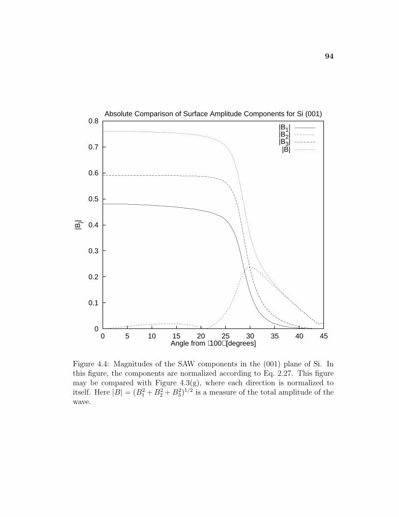
94
0
0.1
0.2
0.3
0.4
0.5
0.6
0.7
0.8
0 5 10 15 20 25 30 35 40 45
|Bj|
Angle from ⟨100⟩ [degrees]
Absolute Comparison of Surface Amplitude Components for Si (001)
|B1||B2||B3||B|
Figure 4.4: Magnitudes of the SAW components in the (001) plane of Si. Inthis figure, the components are normalized according to Eq. 2.27. This figuremay be compared with Figure 4.3(g), where each direction is normalized toitself. Here |B| = (B2
1 + B22 + B2
3)1/2 is a measure of the total amplitude of the
wave.
95
velocity waveform steepen backward in space, and negative segments steepen
forward (i.e., opposite to what a sound wave does in a fluid). In the second re-
gion (20.8◦ < θ < 32.3◦), the nonlinearity is positive, with waveform distortion
the reverse of the first region. In the third region (32.3◦ < θ ≤ 45◦), the non-
linearity is again negative although relatively weak. The standard deviation
divided by the mean for |S11|, |S12|, |S13| ranges between 85%–95% over the
angular range shown. In contrast, the standard deviation divided by the mean
for the linear wave speed is around 2% [see Figure 4.3(d)]. Hence not only do
the nonlinear matrix elements change sign (with distinctly different waveform
evolution as a result) but they also vary more widely in magnitude.
Observe that the weakening in the third region is coincident with the
gradual convergence of the SAW mode and transverse bulk mode into an ex-
ceptional bulk wave as seen from the wave speed plot in Figure 4.3(d). This
can also be seen in Figure 4.3(g) where the transverse component grows relative
to the other two. However, as described above, Figure 4.3(g) normalizes each
direction independently. Figure 4.4 shows the absolute magnitudes of the sur-
face components [only normalized by Eq. 2.27] and indicates that an increasing
amount of energy moves away from the surface and into the bulk of the solid
as the 45◦ direction is approached. As a result, it becomes increasingly difficult
to create the surface amplitudes necessary to observe nonlinear effects in this
real SAW mode.∗
Finally, Figure 4.3(a) indicates that S11, S12, S13 pass through zero near
θ ' 20.8◦ and θ ' 32.3◦. Additional calculations show that while all matrix
elements do not go through zero at the same direction, all elements are close
to zero at these angles. Hence propagation is expected to be nearly linear
∗There does, however, exist a pseudosurface wave mode at a higher wave speed.3 In thisdirection, the pseudosurface wave is the mode that is usually excited experimentally (seeAppendix B for more information on pseudosurface waves.).
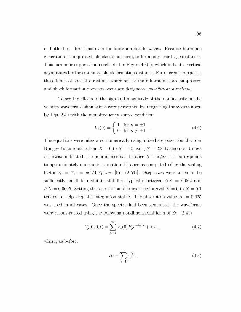
96
in both these directions even for finite amplitude waves. Because harmonic
generation is suppressed, shocks do not form, or form only over large distances.
This harmonic suppression is reflected in Figure 4.3(f), which indicates vertical
asymptotes for the estimated shock formation distance. For reference purposes,
these kinds of special directions where one or more harmonics are suppressed
and shock formation does not occur are designated quasilinear directions.
To see the effects of the sign and magnitude of the nonlinearity on the
velocity waveforms, simulations were performed by integrating the system given
by Eqs. 2.40 with the monofrequency source condition
Vn(0) =
{1 for n = ±10 for n 6= ±1
. (4.6)
The equations were integrated numerically using a fixed step size, fourth-order
Runge–Kutta routine from X = 0 to X = 10 using N = 200 harmonics. Unless
otherwise indicated, the nondimensional distance X = x/x0 = 1 corresponds
to approximately one shock formation distance as computed using the scaling
factor x0 = x11 = ρc4/4|S11|ωv0 [Eq. (2.59)]. Step sizes were taken to be
sufficiently small to maintain stability, typically between ∆X = 0.002 and
∆X = 0.0005. Setting the step size smaller over the interval X = 0 to X = 0.1
tended to help keep the integration stable. The absorption value A1 = 0.025
was used in all cases. Once the spectra had been generated, the waveforms
were reconstructed using the following nondimensional form of Eq. (2.41)
Vj(0, 0, t) =
∞∑n=1
Vn(0)Bje−inωt + c.c. , (4.7)
where, as before,
Bj =3∑
s=1
β(s)j . (4.8)
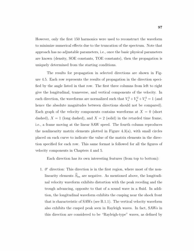
97
However, only the first 150 harmonics were used to reconstruct the waveform
to minimize numerical effects due to the truncation of the spectrum. Note that
approach has no adjustable parameters, i.e., once the basic physical parameters
are known (density, SOE constants, TOE constants), then the propagation is
uniquely determined from the starting conditions.
The results for propagation in selected directions are shown in Fig-
ure 4.5. Each row represents the results of propagation in the direction speci-
fied by the angle listed in that row. The first three columns from left to right
give the longitudinal, transverse, and vertical components of the velocity. In
each direction, the waveforms are normalized such that V 2x +V 2
y +V 2z = 1 (and
hence the absolute magnitudes between directions should not be compared).
Each graph of the velocity components contains waveforms at X = 0 (short
dashed), X = 1 (long dashed), and X = 2 (solid) in the retarded time frame,
i.e., a frame moving at the linear SAW speed. The fourth column reproduces
the nonlinearity matrix elements plotted in Figure 4.3(a), with small circles
placed on each curve to indicate the value of the matrix elements in the direc-
tion specified for each row. This same format is followed for all the figures of
velocity components in Chapters 4 and 5.
Each direction has its own interesting features (from top to bottom):
1. 0◦ direction: This direction is in the first region, where most of the non-
linearity elements Slm are negative. As mentioned above, the longitudi-
nal velocity waveform exhibits distortion with the peak receding and the
trough advancing, opposite to that of a sound wave in a fluid. In addi-
tion, the longitudinal waveform exhibits the cusping near the shock front
that is characteristic of SAWs (see B.1.1). The vertical velocity waveform
also exhibits the cusped peak seen in Rayleigh waves. In fact, SAWs in
this direction are considered to be “Rayleigh-type” waves, as defined by
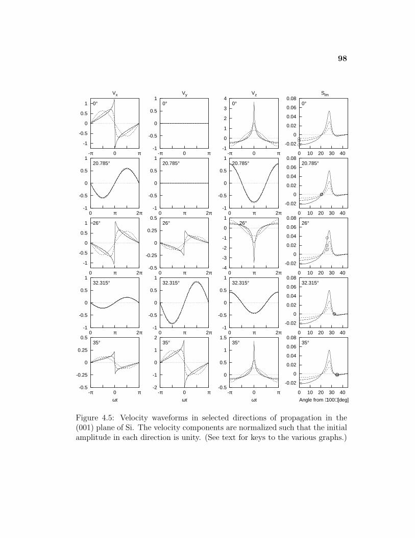
98
-1
-0.5
0
0.5
1
-π 0 π
0°
Vx
-1
-0.5
0
0.5
1
-π 0 π
0°
Vy
-1
0
1
2
3
4
-π 0 π
0°
Vz
-0.02
0
0.02
0.04
0.06
0.08
0 10 20 30 40
Slm
0°
-1
-0.5
0
0.5
1
0 π 2π
20.785°
-1
-0.5
0
0.5
1
0 π 2π
20.785°
-1
-0.5
0
0.5
1
0 π 2π
20.785°
-0.02
0
0.02
0.04
0.06
0.08
0 10 20 30 40
20.785°
-1
-0.5
0
0.5
1
0 π 2π
26°
-0.5
-0.25
0
0.25
0.5
0 π 2π
26°
-4
-3
-2
-1
0
1
0 π 2π
26°
-0.02
0
0.02
0.04
0.06
0.08
0 10 20 30 40
26°
-1
-0.5
0
0.5
1
0 π 2π
32.315°
-1
-0.5
0
0.5
1
0 π 2π
32.315°
-1
-0.5
0
0.5
1
0 π 2π
32.315°
-0.02
0
0.02
0.04
0.06
0.08
0 10 20 30 40
32.315°
-0.5
-0.25
0
0.25
0.5
-π 0 π
35°
ωτ
-2
-1
0
1
2
-π 0 π
35°
ωτ
-0.5
0
0.5
1
1.5
-π 0 π
35°
ωτ
-0.02
0
0.02
0.04
0.06
0.08
0 10 20 30 40
35°
Angle from ⟨100⟩ [deg]
Nor
mal
ized
Vel
ocity
Wav
efor
ms
in (
001)
Pla
ne fo
r S
i
Figure 4.5: Velocity waveforms in selected directions of propagation in the(001) plane of Si. The velocity components are normalized such that the initialamplitude in each direction is unity. (See text for keys to the various graphs.)
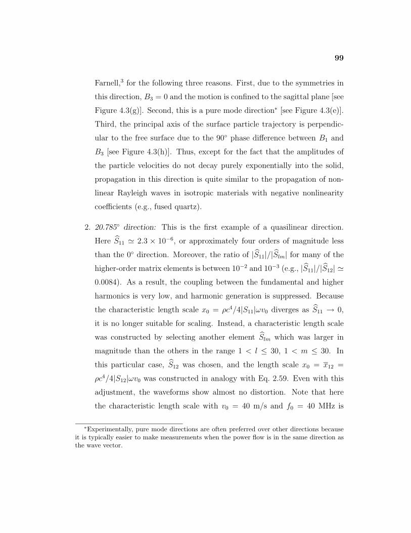
99
Farnell,3 for the following three reasons. First, due to the symmetries in
this direction, B3 = 0 and the motion is confined to the sagittal plane [see
Figure 4.3(g)]. Second, this is a pure mode direction∗ [see Figure 4.3(e)].
Third, the principal axis of the surface particle trajectory is perpendic-
ular to the free surface due to the 90◦ phase difference between B1 and
B3 [see Figure 4.3(h)]. Thus, except for the fact that the amplitudes of
the particle velocities do not decay purely exponentially into the solid,
propagation in this direction is quite similar to the propagation of non-
linear Rayleigh waves in isotropic materials with negative nonlinearity
coefficients (e.g., fused quartz).
2. 20.785◦ direction: This is the first example of a quasilinear direction.
Here S11 ' 2.3 × 10⁻⁶, or approximately four orders of magnitude less
than the 0◦ direction. Moreover, the ratio of |S11|/|Slm| for many of the
higher-order matrix elements is between 10−2 and 10−3 (e.g., |S11|/|S12| '0.0084). As a result, the coupling between the fundamental and higher
harmonics is very low, and harmonic generation is suppressed. Because
the characteristic length scale x0 = ρc4/4|S11|ωv0 diverges as S11 → 0,
it is no longer suitable for scaling. Instead, a characteristic length scale
was constructed by selecting another element Slm which was larger in
magnitude than the others in the range 1 < l ≤ 30, 1 < m ≤ 30. In
this particular case, S12 was chosen, and the length scale x0 = x12 =
ρc4/4|S12|ωv0 was constructed in analogy with Eq. 2.59. Even with this
adjustment, the waveforms show almost no distortion. Note that here
the characteristic length scale with v0 = 40 m/s and f0 = 40 MHz is
∗Experimentally, pure mode directions are often preferred over other directions becauseit is typically easier to make measurements when the power flow is in the same direction asthe wave vector.
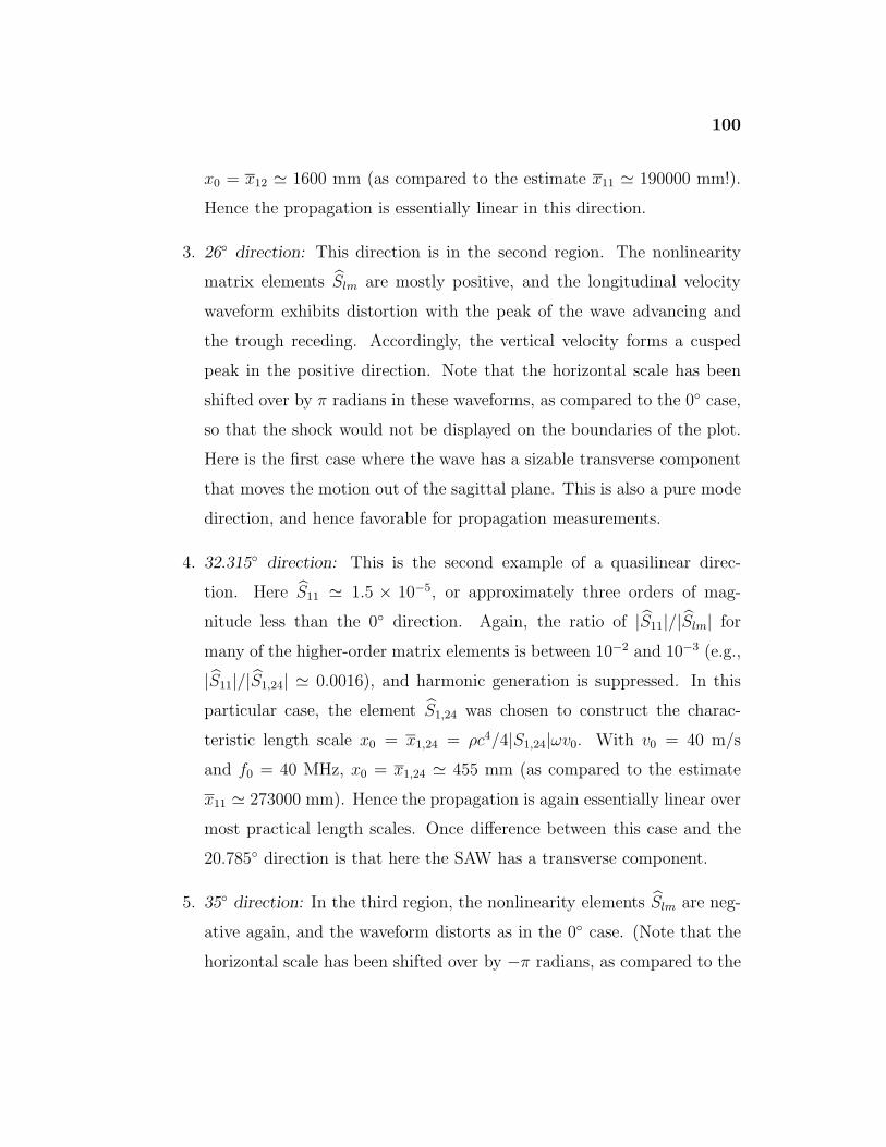
100
x0 = x12 ' 1600 mm (as compared to the estimate x11 ' 190000 mm!).
Hence the propagation is essentially linear in this direction.
3. 26◦ direction: This direction is in the second region. The nonlinearity
matrix elements Slm are mostly positive, and the longitudinal velocity
waveform exhibits distortion with the peak of the wave advancing and
the trough receding. Accordingly, the vertical velocity forms a cusped
peak in the positive direction. Note that the horizontal scale has been
shifted over by π radians in these waveforms, as compared to the 0◦ case,
so that the shock would not be displayed on the boundaries of the plot.
Here is the first case where the wave has a sizable transverse component
that moves the motion out of the sagittal plane. This is also a pure mode
direction, and hence favorable for propagation measurements.
4. 32.315◦ direction: This is the second example of a quasilinear direc-
tion. Here S11 ' 1.5 × 10⁻⁵, or approximately three orders of mag-
nitude less than the 0◦ direction. Again, the ratio of |S11|/|Slm| for
many of the higher-order matrix elements is between 10−2 and 10−3 (e.g.,
|S11|/|S1,24| ' 0.0016), and harmonic generation is suppressed. In this
particular case, the element S1,24 was chosen to construct the charac-
teristic length scale x0 = x1,24 = ρc4/4|S1,24|ωv0. With v0 = 40 m/s
and f0 = 40 MHz, x0 = x1,24 ' 455 mm (as compared to the estimate
x11 ' 273000 mm). Hence the propagation is again essentially linear over
most practical length scales. Once difference between this case and the
20.785◦ direction is that here the SAW has a transverse component.
5. 35◦ direction: In the third region, the nonlinearity elements Slm are neg-
ative again, and the waveform distorts as in the 0◦ case. (Note that the
horizontal scale has been shifted over by −π radians, as compared to the
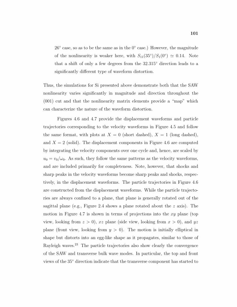
101
26◦ case, so as to be the same as in the 0◦ case.) However, the magnitude
of the nonlinearity is weaker here, with S11(35◦)/S1(0◦) ' 0.14. Note
that a shift of only a few degrees from the 32.315◦ direction leads to a
significantly different type of waveform distortion.
Thus, the simulations for Si presented above demonstrate both that the SAW
nonlinearity varies significantly in magnitude and direction throughout the
(001) cut and that the nonlinearity matrix elements provide a “map” which
can characterize the nature of the waveform distortion.
Figures 4.6 and 4.7 provide the displacement waveforms and particle
trajectories corresponding to the velocity waveforms in Figure 4.5 and follow
the same format, with plots at X = 0 (short dashed), X = 1 (long dashed),
and X = 2 (solid). The displacement components in Figure 4.6 are computed
by integrating the velocity components over one cycle and, hence, are scaled by
u0 = v0/ω0. As such, they follow the same patterns as the velocity waveforms,
and are included primarily for completeness. Note, however, that shocks and
sharp peaks in the velocity waveforms become sharp peaks and shocks, respec-
tively, in the displacement waveforms. The particle trajectories in Figure 4.6
are constructed from the displacement waveforms. While the particle trajecto-
ries are always confined to a plane, that plane is generally rotated out of the
sagittal plane (e.g., Figure 2.4 shows a plane rotated about the z axis). The
motion in Figure 4.7 is shown in terms of projections into the xy plane (top
view, looking from z > 0), xz plane (side view, looking from x > 0), and yz
plane (front view, looking from y > 0). The motion is initially elliptical in
shape but distorts into an egg-like shape as it propagates, similar to those of
Rayleigh waves.23 The particle trajectories also show clearly the convergence
of the SAW and transverse bulk wave modes. In particular, the top and front
views of the 35◦ direction indicate that the transverse component has started to
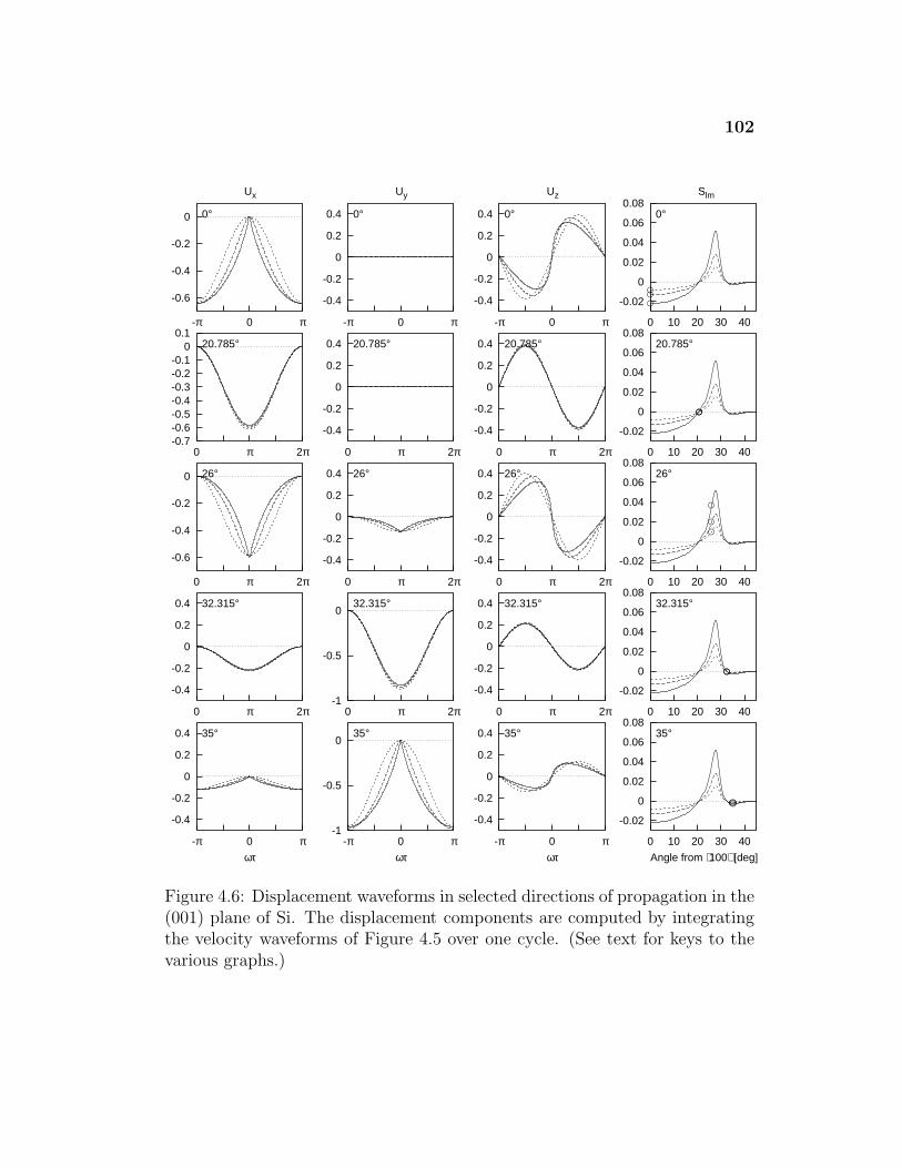
102
-0.6
-0.4
-0.2
0
-π 0 π
0°
Ux
-0.4
-0.2
0
0.2
0.4
-π 0 π
0°
Uy
-0.4
-0.2
0
0.2
0.4
-π 0 π
0°
Uz
-0.02
0
0.02
0.04
0.06
0.08
0 10 20 30 40
Slm
0°
-0.7 -0.6 -0.5 -0.4 -0.3 -0.2 -0.1 0
0.1
0 π 2π
20.785°
-0.4
-0.2
0
0.2
0.4
0 π 2π
20.785°
-0.4
-0.2
0
0.2
0.4
0 π 2π
20.785°
-0.02
0
0.02
0.04
0.06
0.08
0 10 20 30 40
20.785°
-0.6
-0.4
-0.2
0
0 π 2π
26°
-0.4
-0.2
0
0.2
0.4
0 π 2π
26°
-0.4
-0.2
0
0.2
0.4
0 π 2π
26°
-0.02
0
0.02
0.04
0.06
0.08
0 10 20 30 40
26°
-0.4
-0.2
0
0.2
0.4
0 π 2π
32.315°
-1
-0.5
0
0 π 2π
32.315°
-0.4
-0.2
0
0.2
0.4
0 π 2π
32.315°
-0.02
0
0.02
0.04
0.06
0.08
0 10 20 30 40
32.315°
-0.4
-0.2
0
0.2
0.4
-π 0 π
35°
ωτ
-1
-0.5
0
-π 0 π
35°
ωτ
-0.4
-0.2
0
0.2
0.4
-π 0 π
35°
ωτ
-0.02
0
0.02
0.04
0.06
0.08
0 10 20 30 40
35°
Angle from ⟨100⟩ [deg]
Nor
mal
ized
Dis
plac
emen
t Wav
efor
ms
in (
001)
Pla
ne fo
r S
i
Figure 4.6: Displacement waveforms in selected directions of propagation in the(001) plane of Si. The displacement components are computed by integratingthe velocity waveforms of Figure 4.5 over one cycle. (See text for keys to thevarious graphs.)
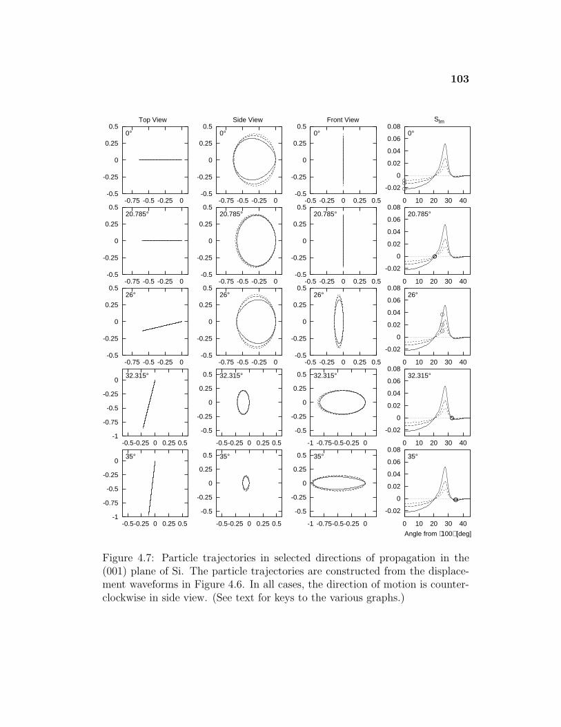
103
-0.5
-0.25
0
0.25
0.5
-0.75 -0.5 -0.25 0
0°
Top View
-0.5
-0.25
0
0.25
0.5
-0.75 -0.5 -0.25 0
0°
Side View
-0.5
-0.25
0
0.25
0.5
-0.5 -0.25 0 0.25 0.5
0°
Front View
-0.02
0
0.02
0.04
0.06
0.08
0 10 20 30 40
Slm
0°
-0.5
-0.25
0
0.25
0.5
-0.75 -0.5 -0.25 0
20.785°
-0.5
-0.25
0
0.25
0.5
-0.75 -0.5 -0.25 0
20.785°
-0.5
-0.25
0
0.25
0.5
-0.5 -0.25 0 0.25 0.5
20.785°
-0.02
0
0.02
0.04
0.06
0.08
0 10 20 30 40
20.785°
-0.5
-0.25
0
0.25
0.5
-0.75 -0.5 -0.25 0
26°
-0.5
-0.25
0
0.25
0.5
-0.75 -0.5 -0.25 0
26°
-0.5
-0.25
0
0.25
0.5
-0.5 -0.25 0 0.25 0.5
26°
-0.02
0
0.02
0.04
0.06
0.08
0 10 20 30 40
26°
-1
-0.75
-0.5
-0.25
0
-0.5-0.25 0 0.25 0.5
32.315°
-0.5
-0.25
0
0.25
0.5
-0.5-0.25 0 0.25 0.5
32.315°
-0.5
-0.25
0
0.25
0.5
-1 -0.75-0.5-0.25 0
32.315°
-0.02
0
0.02
0.04
0.06
0.08
0 10 20 30 40
32.315°
-1
-0.75
-0.5
-0.25
0
-0.5-0.25 0 0.25 0.5
35°
-0.5
-0.25
0
0.25
0.5
-0.5-0.25 0 0.25 0.5
35°
-0.5
-0.25
0
0.25
0.5
-1 -0.75-0.5-0.25 0
35°
-0.02
0
0.02
0.04
0.06
0.08
0 10 20 30 40
35°
Angle from ⟨100⟩ [deg]
Nor
mal
ized
Par
ticle
Tra
ject
orie
s in
(00
1) P
lane
for
Si
Figure 4.7: Particle trajectories in selected directions of propagation in the(001) plane of Si. The particle trajectories are constructed from the displace-ment waveforms in Figure 4.6. In all cases, the direction of motion is counter-clockwise in side view. (See text for keys to the various graphs.)
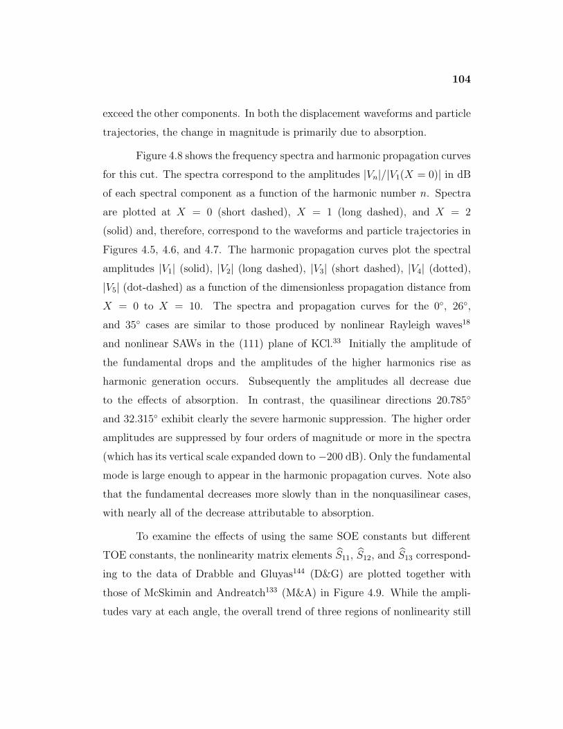
104
exceed the other components. In both the displacement waveforms and particle
trajectories, the change in magnitude is primarily due to absorption.
Figure 4.8 shows the frequency spectra and harmonic propagation curves
for this cut. The spectra correspond to the amplitudes |Vn|/|V1(X = 0)| in dB
of each spectral component as a function of the harmonic number n. Spectra
are plotted at X = 0 (short dashed), X = 1 (long dashed), and X = 2
(solid) and, therefore, correspond to the waveforms and particle trajectories in
Figures 4.5, 4.6, and 4.7. The harmonic propagation curves plot the spectral
amplitudes |V1| (solid), |V2| (long dashed), |V3| (short dashed), |V4| (dotted),
|V5| (dot-dashed) as a function of the dimensionless propagation distance from
X = 0 to X = 10. The spectra and propagation curves for the 0◦, 26◦,
and 35◦ cases are similar to those produced by nonlinear Rayleigh waves18
and nonlinear SAWs in the (111) plane of KCl.33 Initially the amplitude of
the fundamental drops and the amplitudes of the higher harmonics rise as
harmonic generation occurs. Subsequently the amplitudes all decrease due
to the effects of absorption. In contrast, the quasilinear directions 20.785◦
and 32.315◦ exhibit clearly the severe harmonic suppression. The higher order
amplitudes are suppressed by four orders of magnitude or more in the spectra
(which has its vertical scale expanded down to −200 dB). Only the fundamental
mode is large enough to appear in the harmonic propagation curves. Note also
that the fundamental decreases more slowly than in the nonquasilinear cases,
with nearly all of the decrease attributable to absorption.
To examine the effects of using the same SOE constants but different
TOE constants, the nonlinearity matrix elements S11, S12, and S13 correspond-
ing to the data of Drabble and Gluyas144 (D&G) are plotted together with
those of McSkimin and Andreatch133 (M&A) in Figure 4.9. While the ampli-
tudes vary at each angle, the overall trend of three regions of nonlinearity still
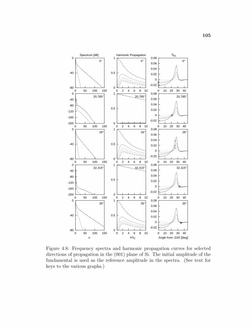
105
-80
-40
0
0 50 100 150
0°
Spectrum [dB]
0
0.5
1
0 2 4 6 8 10
0°
Harmonic Propagation
-0.02
0
0.02
0.04
0.06
0.08
0 10 20 30 40
Slm
0°
-200
-160
-120
-80
-40
0
0 50 100 150
20.785°
0
0.5
1
0 2 4 6 8 10
20.785°
-0.02
0
0.02
0.04
0.06
0.08
0 10 20 30 40
20.785°
-80
-40
0
0 50 100 150
26°
0
0.5
1
0 2 4 6 8 10
26°
-0.02
0
0.02
0.04
0.06
0.08
0 10 20 30 40
26°
-200
-160
-120
-80
-40
0
0 50 100 150
32.315°
0
0.5
1
0 2 4 6 8 10
32.315°
-0.02
0
0.02
0.04
0.06
0.08
0 10 20 30 40
32.315°
-80
-40
0
0 50 100 150
35°
n
0
0.5
1
0 2 4 6 8 10
35°
x/x0
-0.02
0
0.02
0.04
0.06
0.08
0 10 20 30 40
35°
Angle from ⟨100⟩ [deg]
Spe
ctra
and
Har
mon
ic P
ropa
gatio
n C
urve
s in
(00
1) P
lane
for
Si
Figure 4.8: Frequency spectra and harmonic propagation curves for selecteddirections of propagation in the (001) plane of Si. The initial amplitude of thefundamental is used as the reference amplitude in the spectra. (See text forkeys to the various graphs.)
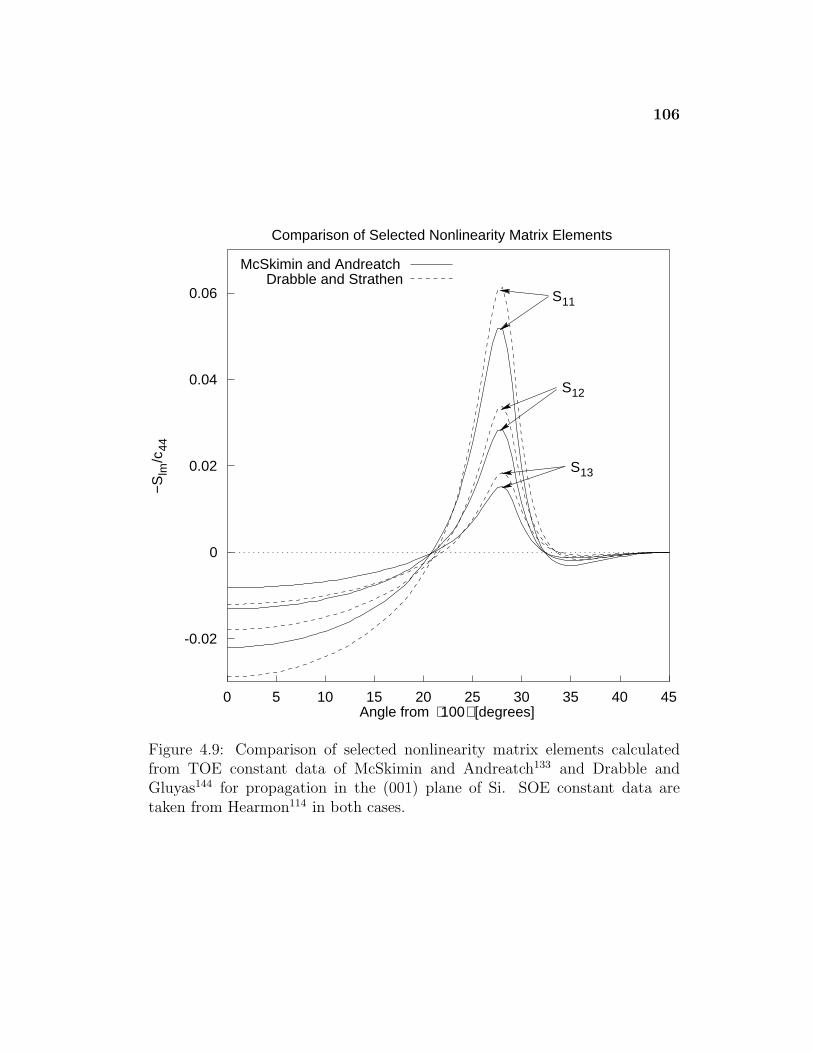
106
-0.02
0
0.02
0.04
0.06
0 5 10 15 20 25 30 35 40 45
−Slm
/c44
Angle from ⟨100⟩ [degrees]
Comparison of Selected Nonlinearity Matrix Elements
S11
S12
S13
McSkimin and AndreatchDrabble and Strathen
Figure 4.9: Comparison of selected nonlinearity matrix elements calculatedfrom TOE constant data of McSkimin and Andreatch133 and Drabble andGluyas144 for propagation in the (001) plane of Si. SOE constant data aretaken from Hearmon114 in both cases.
107
holds. The largest disagreement appears at the extrema. Note also that the
position of the quasilinear directions has shifted a few degrees to the right.
Both sets show directions where the matrix elements cross, although in the
D&G case the crossings do not occur as close to zero as in the M&A case.
In the D&G case, the crossing of the matrix elements occurs at more widely
separated locations. Examination of the nonlinearity matrix elements for other
crystals in Figure 4.2 shows that this separation is probably more common than
the simultaneous crossings of the M&A case. This separated crossing changes
the character of the harmonic generation and waveform distortion as is demon-
strated in the KCl and Ni sections below. Thus, Figure 4.9 indicates that the
detailed waveform predictions for the 20.785◦ and 32.315◦ directions may not
precisely match experimental results. In other words, while the nonlinearity
may be weak in these directions, the resulting waveforms may not be as close to
linear as Figure 4.5 would indicate. Nevertheless, these simulations serve well
the purpose of demonstrating the phenomenon of almost complete suppression
of harmonic generation due to nonlinear effects.
4.2.3 Study of KCl
Additional phenomena can be observed in KCl. Because the linear properties
of KCl are discussed in detail in the review by Farnell,3 they only are discussed
here in so far as they affect the nonlinear properties. Figure 4.10 shows the
nonlinear and linear parameters for KCl in the same format as Figure 4.3 for
Si. As compared to Figure 4.3(a), Figure 4.10(a) for KCl is quantitatively and
qualitatively different. At 0◦, S11 and S12 are positive while S13 and most of
the other elements Slm are negative. As the angle from 〈100〉 increases, S12
goes through zero around 3.205◦ and then finally S11 goes through zero around
5.24◦. At larger angles, most of the matrix elements Slm are negative, although,
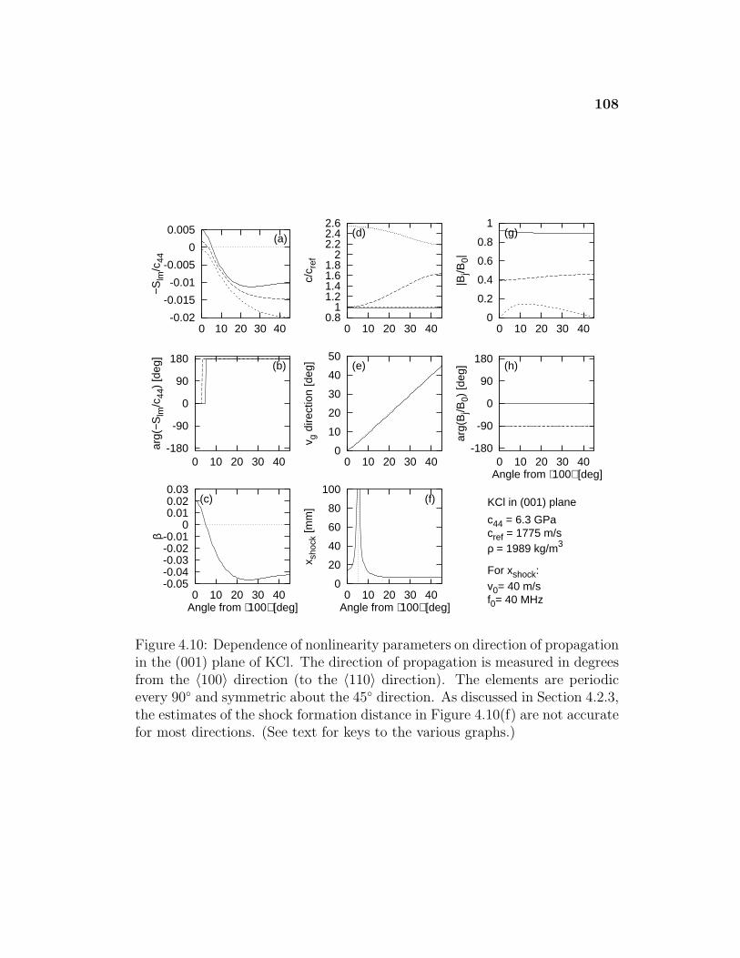
108
-0.02
-0.015
-0.01
-0.005
0
0.005
0 10 20 30 40
−Slm
/c44
(a)
-180
-90
0
90
180
0 10 20 30 40
arg(
−Slm
/c44
) [d
eg]
(b)
-0.05-0.04-0.03-0.02-0.01
0 0.01 0.02 0.03
0 10 20 30 40
β
(c)
Angle from ⟨100⟩ [deg]
0.8 1
1.2 1.4 1.6 1.8 2
2.2 2.4 2.6
0 10 20 30 40
c/c r
ef
(d)
0
10
20
30
40
50
0 10 20 30 40
v g d
irect
ion
[deg
] (e)
0
20
40
60
80
100
0 10 20 30 40
x sho
ck [m
m]
(f)
Angle from ⟨100⟩ [deg]
0
0.2
0.4
0.6
0.8
1
0 10 20 30 40
|Bj/B
0|
(g)
-180
-90
0
90
180
0 10 20 30 40ar
g(B
j/B0)
[deg
] (h)
Angle from ⟨100⟩ [deg]
KCl in (001) plane
c44 = 6.3 GPacref = 1775 m/sρ = 1989 kg/m3
For xshock:v0= 40 m/sf0= 40 MHz
Figure 4.10: Dependence of nonlinearity parameters on direction of propagationin the (001) plane of KCl. The direction of propagation is measured in degreesfrom the 〈100〉 direction (to the 〈110〉 direction). The elements are periodicevery 90◦ and symmetric about the 45◦ direction. As discussed in Section 4.2.3,the estimates of the shock formation distance in Figure 4.10(f) are not accuratefor most directions. (See text for keys to the various graphs.)
109
unlike Si, here the magnitude of S11 is less than the magnitudes of S12, S13,
and other matrix elements. Unlike Si, the SAW modes do not converge with
the transverse bulk mode at 45◦. Finally, the standard deviation divided by
the mean for |S11|, |S12|, |S13| ranges between 38%–45% over the angular range
shown. In contrast, the standard deviation divided by the mean for the linear
wave speed is around 0.2% [see Figure 4.3(d)].
Figures 4.11 and 4.12 show the velocity waveforms, frequency spectra,
and harmonic propagation curves for KCl. Several directions are selected for
consideration in detail:
1. 0◦ direction: In this direction, S11 and S12 are positive, and S13 '7.0 × 10⁻⁴ is negative but close to zero and smaller than S11 and S12
in magnitude (|S13|/|S11| ' 0.14, |S13|/|S12| ' 0.42). The matrix ele-
ment S13 describes the coupling strength between the fundamental and
third harmonic to generate the fourth harmonic. This suppression of
fourth harmonic generation can be seen in the harmonic propagation
curves in Figure 4.12. Energy that is transferred to the third harmonic
from lower harmonics is not as easily transferred to the fourth harmonic.
The third harmonic (short dashed) curve exceeds the second harmonic
(long dashed) in amplitude around X = 3, while the fourth harmonic
grows more slowly initially (as compared to the propagation curves for
the nonquasilinear directions in Si). The trapping of energy in the lowest
harmonics is also reflected in the multiple peaks in the frequency spec-
trum (note expanded vertical scale to −200 dB). Another consequence of
a small value of S13 is that shock formation does not occur. For example,
while the longitudinal waveform shown in Figure 4.12 is distorting in a
“positive” way, with peaks advancing and troughs receding, it has not
yet formed a shock. Additional calculations indicate that at distances
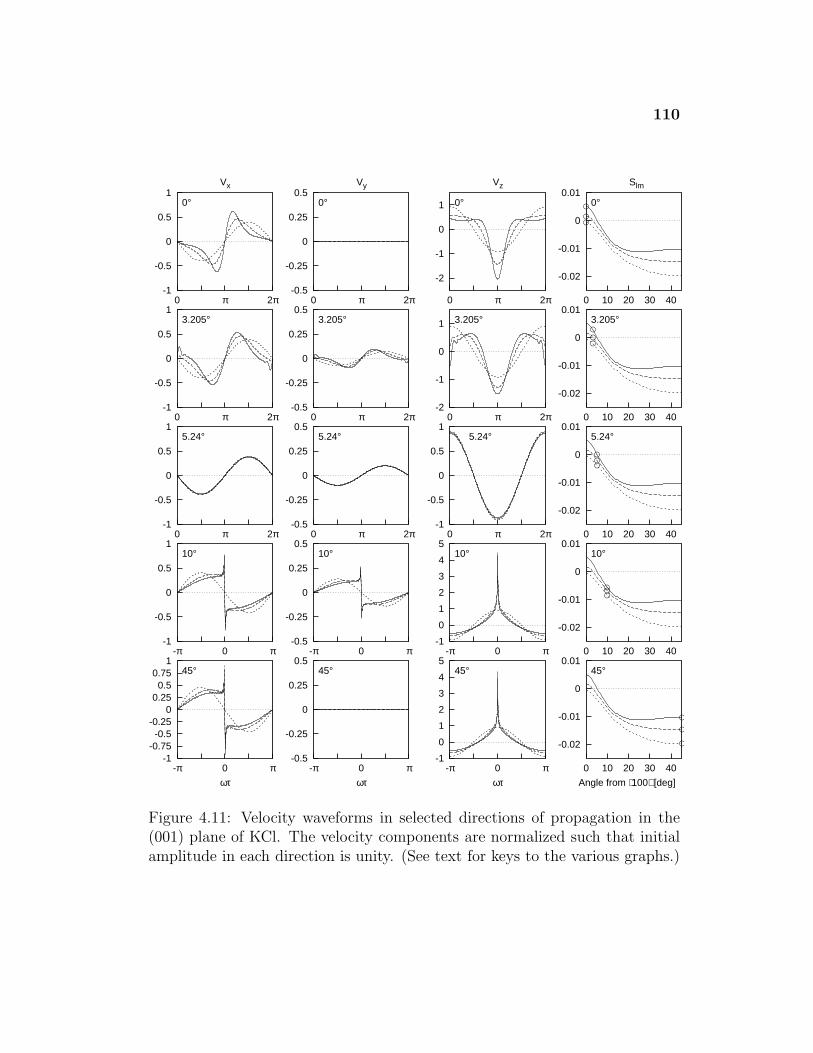
110
-1
-0.5
0
0.5
1
0 π 2π
0°
Vx
-0.5
-0.25
0
0.25
0.5
0 π 2π
0°
Vy
-2
-1
0
1
0 π 2π
0°
Vz
-0.02
-0.01
0
0.01
0 10 20 30 40
Slm
0°
-1
-0.5
0
0.5
1
0 π 2π
3.205°
-0.5
-0.25
0
0.25
0.5
0 π 2π
3.205°
-2
-1
0
1
0 π 2π
3.205°
-0.02
-0.01
0
0.01
0 10 20 30 40
3.205°
-1
-0.5
0
0.5
1
0 π 2π
5.24°
-0.5
-0.25
0
0.25
0.5
0 π 2π
5.24°
-1
-0.5
0
0.5
1
0 π 2π
5.24°
-0.02
-0.01
0
0.01
0 10 20 30 40
5.24°
-1
-0.5
0
0.5
1
-π 0 π
10°
-0.5
-0.25
0
0.25
0.5
-π 0 π
10°
-1
0
1
2
3
4
5
-π 0 π
10°
-0.02
-0.01
0
0.01
0 10 20 30 40
10°
-1-0.75 -0.5
-0.25 0
0.25 0.5
0.75 1
-π 0 π
45°
ωτ
-0.5
-0.25
0
0.25
0.5
-π 0 π
45°
ωτ
-1
0
1
2
3
4
5
-π 0 π
45°
ωτ
-0.02
-0.01
0
0.01
0 10 20 30 40
45°
Angle from ⟨100⟩ [deg]
Nor
mal
ized
Vel
ocity
Wav
efor
ms
in (
001)
Pla
ne fo
r K
Cl
Figure 4.11: Velocity waveforms in selected directions of propagation in the(001) plane of KCl. The velocity components are normalized such that initialamplitude in each direction is unity. (See text for keys to the various graphs.)
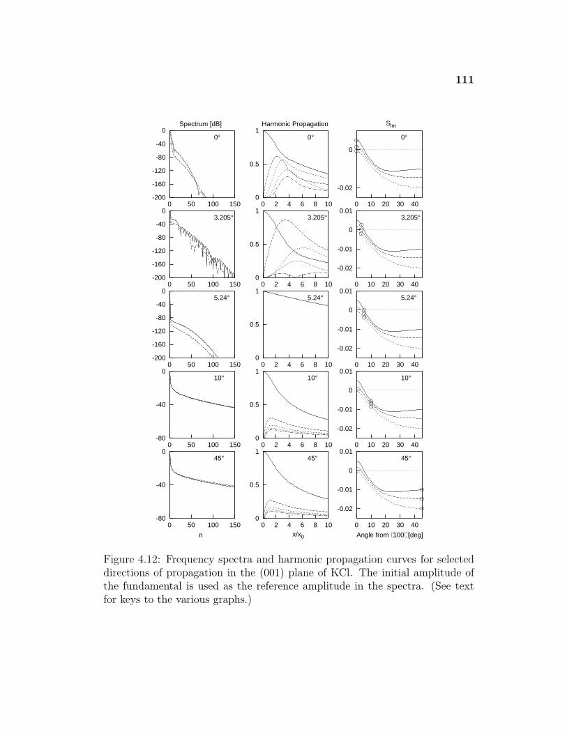
111
-200
-160
-120
-80
-40
0
0 50 100 150
0°
Spectrum [dB]
0
0.5
1
0 2 4 6 8 10
0°
Harmonic Propagation
-0.02
0
0 10 20 30 40
Slm
0°
-200
-160
-120
-80
-40
0
0 50 100 150
3.205°
0
0.5
1
0 2 4 6 8 10
3.205°
-0.02
-0.01
0
0.01
0 10 20 30 40
3.205°
-200
-160
-120
-80
-40
0
0 50 100 150
5.24°
0
0.5
1
0 2 4 6 8 10
5.24°
-0.02
-0.01
0
0.01
0 10 20 30 40
5.24°
-80
-40
0
0 50 100 150
10°
0
0.5
1
0 2 4 6 8 10
10°
-0.02
-0.01
0
0.01
0 10 20 30 40
10°
-80
-40
0
0 50 100 150
45°
n
0
0.5
1
0 2 4 6 8 10
45°
x/x0
-0.02
-0.01
0
0.01
0 10 20 30 40
45°
Angle from ⟨100⟩ [deg]
Spe
ctra
and
Har
mon
ic P
ropa
gatio
n C
urve
s in
(00
1) P
lane
for
KC
l
Figure 4.12: Frequency spectra and harmonic propagation curves for selecteddirections of propagation in the (001) plane of KCl. The initial amplitude ofthe fundamental is used as the reference amplitude in the spectra. (See textfor keys to the various graphs.)
112
X > 2 the longitudinal velocity waveform steepens more but does not
ever form a shock. Hence this is another quasilinear direction, although
with a somewhat different character than those described for Si because
the harmonic suppression is less severe and occurs in a harmonic higher
than the second.
2. 3.205◦ direction: Here S11 is positive, S12 ' −5.9×10⁻⁷ is close zero, and
S13 and most other matrix elements Slm are negative. In addition S12 is
smaller than S11 in magnitude (|S13|/|S11| ' 2.1× 10⁻⁴). The matrix el-
ement S12 describes the coupling strength between the fundamental and
second harmonic to generate the third harmonic. The suppression of third
harmonic generation can be seen in the harmonic propagation curves in
Figure 4.12. The second harmonic (long dashed) grows to be larger in
amplitude than the fundamental (solid) around X = 2, and the third and
higher harmonics grow more slowly initially. The trapping of energy in
the lowest harmonics leads to other unusual phenomena, including the
amplitude of the third harmonic (short dashed) exceeding the fundamen-
tal past X = 5, and the suppression of fourth harmonic (dotted) around
the same location. The complicated interaction of the lowest harmonics
is also reflected in the spectra which have many peaks and valleys at
both X = 1 (long dashed) and X = 2 (short dashed). The waveforms
of Figure 4.11 do not exhibit shock formation but do show some higher
frequency oscillations due to the atypical energy trapping and unusual
spectral structure. (The shown oscillations are not due to spectrum trun-
cation or Gibbs oscillations from the numerical calculations.) Additional
calculations show that at distances X > 2 the waveform does not form
a shock, and the higher frequency oscillations grow in extent and magni-
tude. As mentioned in Section 2.2.4, the amplitudes of the fundamental
113
and second harmonic for this direction can be modelled approximately
for distances X ≤ 2 by a coupled two-mode system.33 In summary, the
simulations identify the 3.205◦ direction as another quasilinear direction,
although with a still different character than either of those described for
Si or for the 0◦ case in KCl above.
3. 5.24◦ direction: This is another example of a quasilinear direction like
the cases of Si. The matrix element S11 ' −1.249× 10⁻⁶ is close to zero
and small compared to neighboring elements (e.g., |S11|/|S12| ' 0.0006).
Hence second harmonic generation is suppressed and propagation is es-
sentially linear. In this particular case, the element S1,8 was chosen to
construct the characteristic length scale x0 = x1,8 = ρc4/4|S1,8|ωv0. With
v0 = 40 m/s and f0 = 40 MHz, x0 = x1,8 ' 12 mm (as compared to the
estimate x11 ' 59000 mm).
4. 10◦ direction: Here most of the nonlinearity matrix elements Slm are
negative, but, unlike the 0◦ and 35◦ directions in Si, here the magni-
tude |S11| is less than neighboring elements (e.g., |S11|/|S12| ' 0.84 and
|S11|/|S12| ' 0.68). As can be seen from the spectrum, this inversion in
the magnitudes of the matrix elements causes energy to be transferred
to the higher harmonics at a faster rate (compared the X = 1 curves in
Si to this case). In turn, this increased rate of energy transfer results in
significantly sharper cusping in the waveforms.
5. 45◦ direction: This case is very similar to the 10◦ direction. However,
propagation in this direction occurs in a pure mode (see Figure 4.10(e)).
In summary, the simulations for KCl in the (001) plane indicate that (1) several
different varieties of quasilinear directions exist and (2) care should be taken
with the simple estimate of the shock formation distance given by Eq. (2.59)
114
for all directions in this cut. Note that in both quasilinear cases (e.g., 0◦ and
3.205◦ directions) and matrix element inversion cases (e.g., 10◦ and 45◦) the
simplistic estimate of the shock formation distance x11 = ρc4/4|S11|ωv0 proba-
bly underestimates or overestimates, respectively, the characteristic nonlinear
length scale. Therefore, the values given in Figure 4.10(f) are not accurate for
most directions.
Finally, the effect of different experimental TOE constants is examined.
Figure 4.13 shows a comparison between the nonlinearity elements computed
using the data of Drabble and Strathen128 (used in the simulations above)
and Chang.127 Both sets show the same trend decreasing from positive to
negative, but the location of the zero crossings shifts to the left. In particular,
the 0◦ direction with the Chang data has the same character as the 3.205◦
case with the Drabble and Strathen data. Because Hamilton et al.33 used
the Chang data to perform their simulations for KCl, their paper shows these
more unusual waveforms and spectra in the 0◦ direction. An examination of
Chang’s paper shows that only three of the six TOE constants were determined
experimentally (d144, d155, d456) while the other elastic constants (d111, d122,
d123) were computed by assuming the Cauchy relations d123 = d456 = d144 and
d112 = d166. In contrast, Drabble and Strathen measured all six constants and
showed that not all the Cauchy relations hold (see Table 3.4). In any case,
the lesson here is that the nonlinearity matrix elements and, therefore, the
waveform distortion are fairly sensitive to changes in the TOE constants. Thus
care should be exercised in making detailed predictions about specific directions
without good TOE constant data.
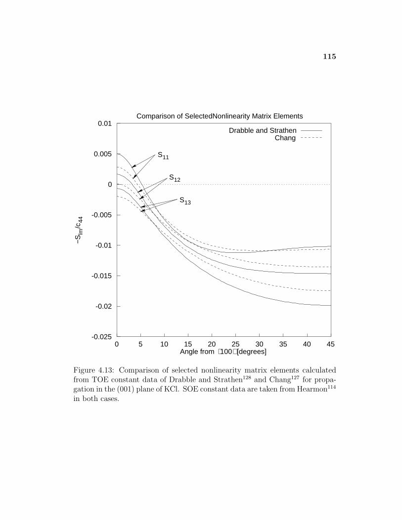
115
-0.025
-0.02
-0.015
-0.01
-0.005
0
0.005
0.01
0 5 10 15 20 25 30 35 40 45
−/c
44
Angle from ⟨100⟩ [degrees]
Comparison of SelectedNonlinearity Matrix Elements
Chang
Slm
S11
S12
S13
Drabble and Strathen
Figure 4.13: Comparison of selected nonlinearity matrix elements calculatedfrom TOE constant data of Drabble and Strathen128 and Chang127 for propa-gation in the (001) plane of KCl. SOE constant data are taken from Hearmon114
in both cases.
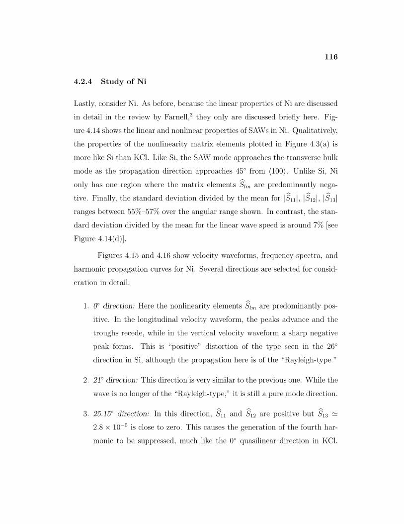
116
4.2.4 Study of Ni
Lastly, consider Ni. As before, because the linear properties of Ni are discussed
in detail in the review by Farnell,3 they only are discussed briefly here. Fig-
ure 4.14 shows the linear and nonlinear properties of SAWs in Ni. Qualitatively,
the properties of the nonlinearity matrix elements plotted in Figure 4.3(a) is
more like Si than KCl. Like Si, the SAW mode approaches the transverse bulk
mode as the propagation direction approaches 45◦ from 〈100〉. Unlike Si, Ni
only has one region where the matrix elements Slm are predominantly nega-
tive. Finally, the standard deviation divided by the mean for |S11|, |S12|, |S13|ranges between 55%–57% over the angular range shown. In contrast, the stan-
dard deviation divided by the mean for the linear wave speed is around 7% [see
Figure 4.14(d)].
Figures 4.15 and 4.16 show velocity waveforms, frequency spectra, and
harmonic propagation curves for Ni. Several directions are selected for consid-
eration in detail:
1. 0◦ direction: Here the nonlinearity elements Slm are predominantly pos-
itive. In the longitudinal velocity waveform, the peaks advance and the
troughs recede, while in the vertical velocity waveform a sharp negative
peak forms. This is “positive” distortion of the type seen in the 26◦
direction in Si, although the propagation here is of the “Rayleigh-type.”
2. 21◦ direction: This direction is very similar to the previous one. While the
wave is no longer of the “Rayleigh-type,” it is still a pure mode direction.
3. 25.15◦ direction: In this direction, S11 and S12 are positive but S13 '2.8× 10⁻⁵ is close to zero. This causes the generation of the fourth har-
monic to be suppressed, much like the 0◦ quasilinear direction in KCl.
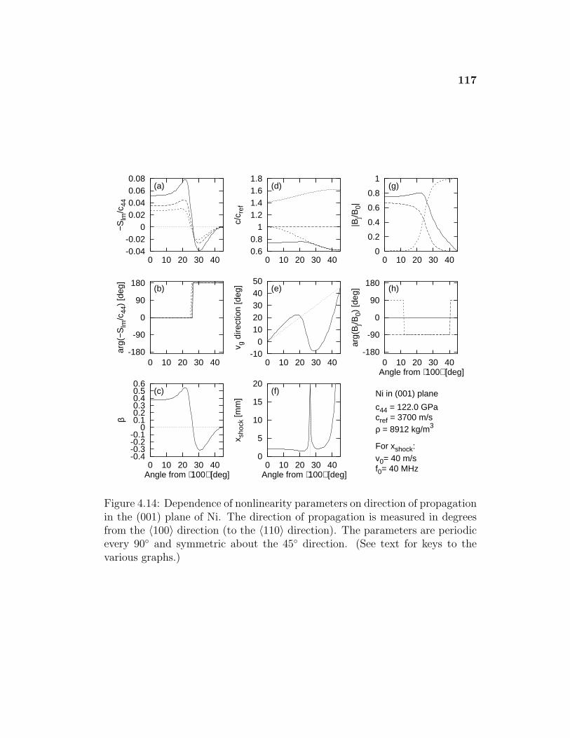
117
-0.04-0.02
0 0.02 0.04 0.06 0.08
0 10 20 30 40
−Slm
/c44
(a)
-180
-90
0
90
180
0 10 20 30 40
arg(
−Slm
/c44
) [d
eg]
(b)
-0.4 -0.3 -0.2 -0.1 0
0.1 0.2 0.3 0.4 0.5 0.6
0 10 20 30 40
β
(c)
Angle from ⟨100⟩ [deg]
0.6 0.8 1
1.2 1.4 1.6 1.8
0 10 20 30 40
c/c r
ef
(d)
-10 0
10 20 30 40 50
0 10 20 30 40
v g d
irect
ion
[deg
] (e)
0
5
10
15
20
0 10 20 30 40
x sho
ck [m
m]
(f)
Angle from ⟨100⟩ [deg]
0
0.2
0.4
0.6
0.8
1
0 10 20 30 40
|Bj/B
0|
(g)
-180
-90
0
90
180
0 10 20 30 40ar
g(B
j/B0)
[deg
] (h)
Angle from ⟨100⟩ [deg]
Ni in (001) plane
c44 = 122.0 GPacref = 3700 m/sρ = 8912 kg/m3
For xshock:v0= 40 m/sf0= 40 MHz
Figure 4.14: Dependence of nonlinearity parameters on direction of propagationin the (001) plane of Ni. The direction of propagation is measured in degreesfrom the 〈100〉 direction (to the 〈110〉 direction). The parameters are periodicevery 90◦ and symmetric about the 45◦ direction. (See text for keys to thevarious graphs.)
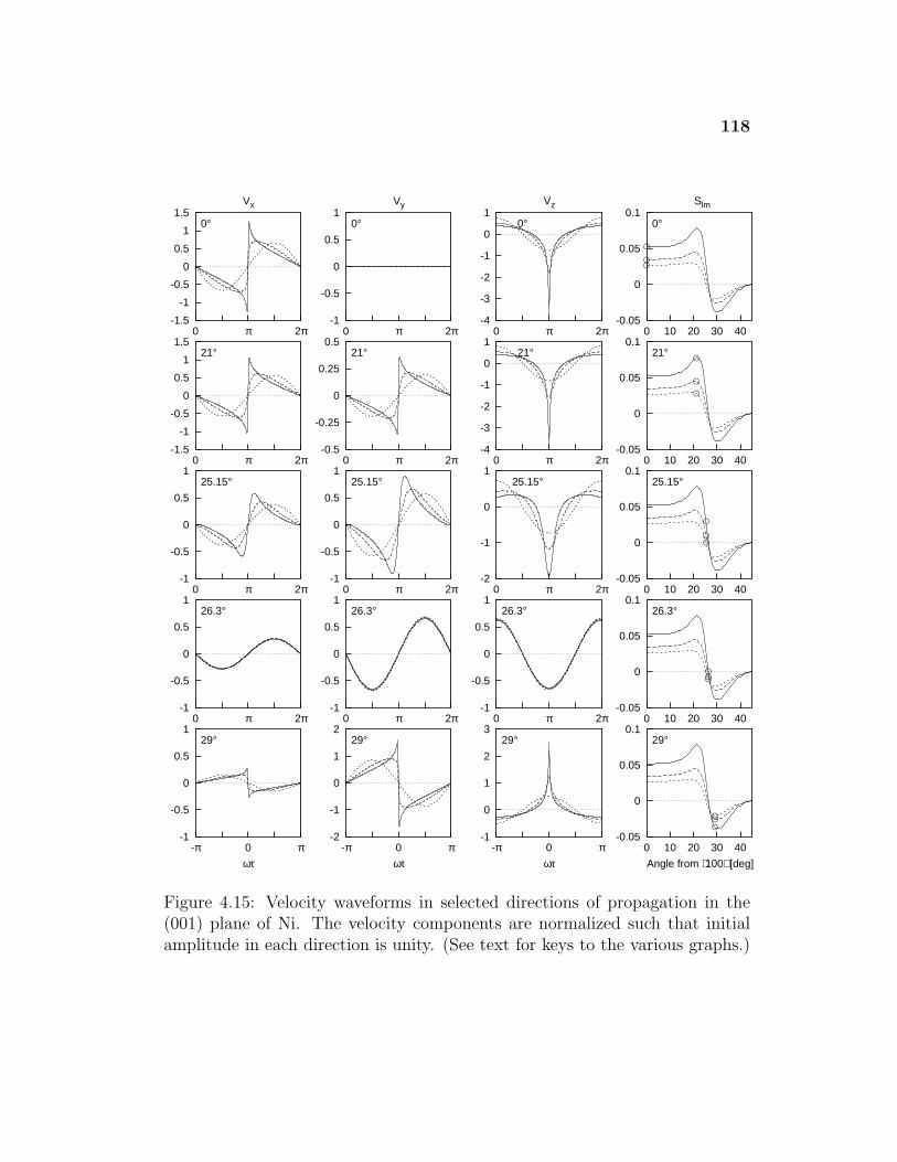
118
-1.5
-1
-0.5
0
0.5
1
1.5
0 π 2π
0°
Vx
-1
-0.5
0
0.5
1
0 π 2π
0°
Vy
-4
-3
-2
-1
0
1
0 π 2π
0°
Vz
-0.05
0
0.05
0.1
0 10 20 30 40
Slm
0°
-1.5
-1
-0.5
0
0.5
1
1.5
0 π 2π
21°
-0.5
-0.25
0
0.25
0.5
0 π 2π
21°
-4
-3
-2
-1
0
1
0 π 2π
21°
-0.05
0
0.05
0.1
0 10 20 30 40
21°
-1
-0.5
0
0.5
1
0 π 2π
25.15°
-1
-0.5
0
0.5
1
0 π 2π
25.15°
-2
-1
0
1
0 π 2π
25.15°
-0.05
0
0.05
0.1
0 10 20 30 40
25.15°
-1
-0.5
0
0.5
1
0 π 2π
26.3°
-1
-0.5
0
0.5
1
0 π 2π
26.3°
-1
-0.5
0
0.5
1
0 π 2π
26.3°
-0.05
0
0.05
0.1
0 10 20 30 40
26.3°
-1
-0.5
0
0.5
1
-π 0 π
29°
ωτ
-2
-1
0
1
2
-π 0 π
29°
ωτ
-1
0
1
2
3
-π 0 π
29°
ωτ
-0.05
0
0.05
0.1
0 10 20 30 40
29°
Angle from ⟨100⟩ [deg]
Nor
mal
ized
Vel
ocity
Wav
efor
ms
in (
001)
Pla
ne fo
r N
i
Figure 4.15: Velocity waveforms in selected directions of propagation in the(001) plane of Ni. The velocity components are normalized such that initialamplitude in each direction is unity. (See text for keys to the various graphs.)
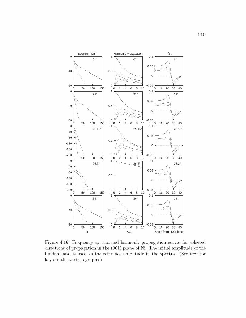
119
-80
-40
0
0 50 100 150
0°
Spectrum [dB]
0
0.5
1
0 2 4 6 8 10
0°
Harmonic Propagation
-0.05
0
0.05
0.1
0 10 20 30 40
Slm
0°
-80
-40
0
0 50 100 150
21°
0
0.5
1
0 2 4 6 8 10
21°
-0.05
0
0.05
0.1
0 10 20 30 40
21°
-200
-160
-120
-80
-40
0
0 50 100 150
25.15°
0
0.5
1
0 2 4 6 8 10
25.15°
-0.05
0
0.05
0.1
0 10 20 30 40
25.15°
-200
-160
-120
-80
-40
0
0 50 100 150
26.3°
0
0.5
1
0 2 4 6 8 10
26.3°
-0.05
0
0.05
0.1
0 10 20 30 40
26.3°
-80
-40
0
0 50 100 150
29°
n
0
0.5
1
0 2 4 6 8 10
29°
x/x0
-0.05
0
0.05
0.1
0 10 20 30 40
29°
Angle from ⟨100⟩ [deg]
Spe
ctra
and
Har
mon
ic P
ropa
gatio
n C
urve
s in
(00
1) P
lane
for
Ni
Figure 4.16: Frequency spectra and harmonic propagation curves for selecteddirections of propagation in the (001) plane of Ni. The initial amplitude of thefundamental is used as the reference amplitude in the spectra. (See text forkeys to the various graphs.)
120
Additional calculations indicate that at distances X > 2 the longitudinal
velocity waveform steepens more but does not form a shock. The har-
monic propagation curves for lowest order harmonics show an increase in
magnitude in the region 0 < X < 3 due to trapping that results from the
suppression, although eventually the third and fourth harmonics reach
the same magnitude.
4. 26.3◦ direction: This is another example of the quasilinear directions like
those seen in the 20.785◦ and 32.315◦ directions in Si. Here the ma-
trix element S11 = 3.3 × 10⁻⁵, and it is small compared to neighboring
elements (e.g., |S11|/|S12| ' 0.0047). As a result, second harmonic gener-
ation is suppressed and the propagation is nearly linear. In this particular
case, the element S1,4 was chosen to construct the characteristic length
scale x0 = x1,8 = ρc4/4|S1,8|ωv0 for the simulation. With v0 = 40 m/s
and f0 = 40 MHz, x0 = x1,8 ' 8.6 mm (as compared to the estimate
x11 ' 3100 mm).
5. 29◦ direction: Here the matrix elements Slm are predominantly negative
and the motion is mostly in the transverse and vertical directions, similar
to the 35◦ direction in Si. (Note that the horizontal scale has been shifted
over by −π radians as compared to the other cases.)
To summarize, this case shows many of the same nonlinear features as seen in
the Si and KCl cases. These similarities occur despite the fact that (1) Si has a
diamond crystalline structure while Ni does not, and (2) KCl has an anisotropy
ratio η < 1 while Ni has anisotropy ratio η < 1. As before, the estimates of
the shock formation distance given in Figure 4.14(f) may be inaccurate in the
vicinity of quasilinear directions like the 25.15◦ direction. However, in contrast
to KCl, the estimates for Ni should be valid for most directions in the plane.
121
Finally, the effect of different experimental TOE constants is examined.
Figure 4.17 shows a comparison between the nonlinearity elements computed
using the data of Salama and Alers136 (used in the simulations above) and
Sarma and Reddy.137 While the curves show the same overall trend, the devi-
ation is larger than in the previous cases. The deviation may be due at least
in part to the fact that data of Sarma and Reddy were taken while the sample
was magnetically saturated.
4.3 Summary
This chapter has investigated the properties of nonlinear SAWs in the (001)
plane of selected crystals. Si, KCl, and Ni were chosen for detailed study. It
is found that the nature of the nonlinearity is often very sensitive to changes
in direction, and the magnitude of the changes can be larger than linear quan-
tities like the wave speed. For most cases, plotting the first few nonlinearity
matrix elements as a function of direction can provide a guide to the nature
of the nonlinear effects. While particular directions of high symmetry exhibit
harmonic generation and waveform distortion similar to Rayleigh waves, sev-
eral other new effects have been identified including (1) the existence of regions
of “positive” and “negative” nonlinearity within the same cut, (2) several va-
rieties of quasilinear directions where the generation of particular harmonics is
suppressed and shock formation does not occur, (3) directions in which shock
formation is enhanced by rapid transfer of energy to the higher harmonics. As
a result of the latter two effects, the simple estimate of the shock formation
given by Eq. (2.59) may not be valid or accurate in some regions. The choice of
different experimental TOE constants as input to the simulations is shown to
affect the detailed predictions of the nonlinearity matrix elements in any given
direction, but not the trends over the whole angular range. Many of the ideas
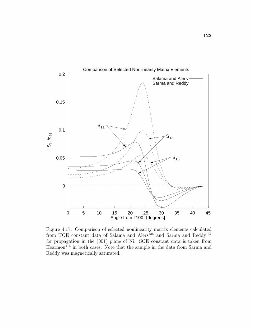
122
0
0.05
0.1
0.15
0.2
0 5 10 15 20 25 30 35 40 45
−Slm
/c44
Angle from ⟨100
S
S
S
⟩
11
12
13
[degrees]
Comparison of Selected Nonlinearity Matrix Elements
Salama and AlersSarma and Reddy
Figure 4.17: Comparison of selected nonlinearity matrix elements calculatedfrom TOE constant data of Salama and Alers136 and Sarma and Reddy137
for propagation in the (001) plane of Ni. SOE constant data is taken fromHearmon114 in both cases. Note that the sample in the data from Sarma andReddy was magnetically saturated.
123
presented in this chapter are further investigated in the next chapter with a
different cut.
Chapter 5
Monofrequency SAWs in the (110) Plane
This chapter describes the propagation of finite amplitude SAWs in the (110)
surface cut. (See Figure D.1 for a diagram of this cut.) The chapter applies the
same type of analysis used in Chapter 4 to describe and explain the linear and
nonlinear properties of surface waves in this plane. Unless otherwise indicated,
the figures in the chapter have the same format as in Chapter 4, and the reader
is referred to that chapter for detailed explanations. The structure of Chapter 4
is also paralleled: (1) a brief review of linear properties, (2) a general study of
a variety of crystals, and (3) a detailed study of Si, KCl, and Ni.
5.1 Linear Effects
Figure 5.1 shows the SAW speed of selected materials as a function of the
propagation direction. The direction of propagation is measured in degrees
from the 〈001〉 direction, and the speed for each material is scaled by the
characteristic speed cref = (c44/ρ)1/2 for that material. Because the normal to
the (110) plane is a twofold symmetry axis, the SAW speed is periodic every
180◦. In addition, the the 〈110〉 direction is a twofold symmetry axis so that
the SAW speed is symmetric about that direction (90◦ in the figure). In most
cases (and for all the cases shown here), the speeds group by anisotropy ratio,
with materials with lower anisotropy ratios having higher relative SAW speeds.
Materials with η ≈ 1 are nearly isotropic, and hence have nearly constant
SAW speed for all directions. The dashed lines indicate the crystals in the
124
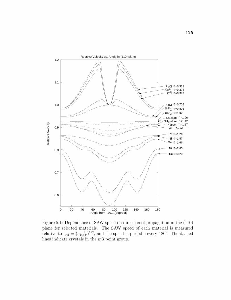
125
0.6
0.7
0.8
0.9
1.0
1.1
1.2
0 20 40 60 80 100 120 140 160 180
Rel
ativ
e V
eloc
ity
Angle from ⟨001⟩ [degrees]
Relative Velocity vs. Angle in (110) plane
η=0.312RbClCaF2 η=0.373
η=0.373KCl
NaCl η=0.705SrF 2 η=0.803
η=1.02BaF2η=1.06Cs-alum
-alum4 η=1.12NHK-alum η=1.17
Al η=1.22
C η=1.26
Si η=1.57Ge η=1.66
Ni η=2.60
Cu η=3.20
Figure 5.1: Dependence of SAW speed on direction of propagation in the (110)plane for selected materials. The SAW speed of each material is measuredrelative to cref = (c44/ρ)1/2, and the speed is periodic every 180◦. The dashedlines indicate crystals in the m3 point group.
126
m3 point group. According to Farnell,3 SAWs propagating in the 0◦ direction
are “Rayleigh-type” waves (like the direction 0◦ from 〈100〉 in Si; see also
Section B.1.3), whereas SAWs in the 90◦ direction are actually simple Rayleigh
waves (“Rayleigh-type” plus non-oscillatory decay into the solid). As a result,
both the 0◦ and 90◦ directions are pure modes. Pure modes may also exist in
other directions depending on the individual crystal.
5.2 Nonlinear Effects
This section shows that:
• The nonlinearity changes in magnitude and sign as a function of direction.
These changes are often proportionally larger than variations of linear
quantities over the same range.
• Quasilinear directions exist where no shock formation occurs even for
finite amplitude waves.
• Directions exist where shock formation is enhanced.
These properties are similar in many ways to those in the (001) plane.
5.2.1 General Study
The same materials are considered here as in Chapter 4. Figure 5.2 displays
the nonlinearity matrix elements for all the materials except the alums, which
are shown in Figure 5.3.
As before, Figure 5.2 shows S11 (solid), S12 (long dashed), and S13 (short
dashed) over the range of directions 0◦ to 45◦ from 〈100〉. The vertical scale on
each plot is adjusted to show the curves most clearly for each material. The
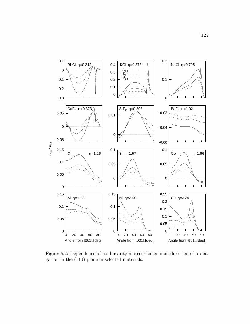
127
-0.3
-0.2
-0.1
0
0.1
RbCl η=0.312
0
0.1
0.2
0.3
0.4
KCl η=0.373S11S12S13
0
0.1
0.2
NaCl η=0.705
-0.05
0
0.05
CaF2 η=0.373
0
0.01
SrF2 η=0.803
-0.06
-0.04
-0.02
BaF2 η=1.02
0
0.05
0.1
0.15
0 20 40 60 80
Al η=1.22
Angle from ⟨001⟩ [deg]
0
0.05
0.1
0.15
0 20 40 60 80
Ni η=2.60
Angle from ⟨001⟩ [deg]
0
0.05
0.1
0.15
0.2
0.25
0 20 40 60 80
Cu η=3.20
Angle from ⟨001⟩ [deg]
0
0.05
0.1
0.15
C η=1.26
0
0.05
0.1
Si η=1.57
0
0.05
0.1
Ge η=1.66
−Slm
/ c 4
4Normalized Nonlinearity Matrix Elements in (110) Plane for Selected Materials
Figure 5.2: Dependence of nonlinearity matrix elements on direction of propa-gation in the (110) plane in selected materials.
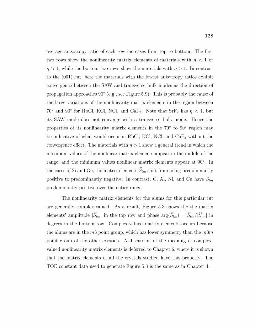
128
average anisotropy ratio of each row increases from top to bottom. The first
two rows show the nonlinearity matrix elements of materials with η < 1 or
η ≈ 1, while the bottom two rows show the materials with η > 1. In contrast
to the (001) cut, here the materials with the lowest anisotropy ratios exhibit
convergence between the SAW and transverse bulk modes as the direction of
propagation approaches 90◦ (e.g., see Figure 5.9). This is probably the cause of
the large variations of the nonlinearity matrix elements in the region between
70◦ and 90◦ for RbCl, KCl, NCl, and CaF2. Note that SrF2 has η < 1, but
its SAW mode does not converge with a transverse bulk mode. Hence the
properties of its nonlinearity matrix elements in the 70◦ to 90◦ region may
be indicative of what would occur in RbCl, KCl, NCl, and CaF2 without the
convergence effect. The materials with η > 1 show a general trend in which the
maximum values of the nonlinear matrix elements appear in the middle of the
range, and the minimum values nonlinear matrix elements appear at 90◦. In
the cases of Si and Ge, the matrix elements Slm shift from being predominantly
positive to predominantly negative. In contrast, C, Al, Ni, and Cu have Slm
predominantly positive over the entire range.
The nonlinearity matrix elements for the alums for this particular cut
are generally complex-valued. As a result, Figure 5.3 shows the the matrix
elements’ amplitude |Slm| in the top row and phase arg(Slm) = Slm/|Slm| in
degrees in the bottom row. Complex-valued matrix elements occurs because
the alums are in the m3 point group, which has lower symmetry than the m3m
point group of the other crystals. A discussion of the meaning of complex-
valued nonlinearity matrix elements is deferred to Chapter 6, where it is shown
that the matrix elements of all the crystals studied have this property. The
TOE constant data used to generate Figure 5.3 is the same as in Chapter 4.
129
0
0.02
0.04
0.06
Cs-alum
0
0.02
0.04
0.06
NH4-alum
0
0.05
0.1
K-alum
-180
-90
0
0 20 40 60 80
Angle from ⟨001⟩ [deg]
-180
-90
0
0 20 40 60 80
Angle from ⟨001⟩ [deg]
-180
-90
0
0 20 40 60 80
Angle from ⟨001⟩ [deg]
arg(
−Slm
/ c 4
4) [d
eg]
|Slm
| / c
44
Normalized Nonlinearity Matrix Elements in (110) Plane for Selected Materials
Figure 5.3: Dependence of nonlinearity matrix elements on direction of propa-gation in the (110) plane in selected materials. S11 (solid), S12 (long dashed),
and S13 (short dashed) are plotted in each graph.
130
5.2.2 Study of Si
Figure 5.4 for the (110) plane of Si is similar to the figures of linear and non-
linear parameters in Chapter 4. Figures 5.5, 5.6, 5.7, and 5.8 show the velocity
waveforms, displacement waveforms, particle trajectories, and frequency spec-
tra plus the harmonic propagation curves, respectively. Figure 5.4(a) shows
that S11, S12, and S13 start out around zero at 0◦, grow to a maximum around
37◦, and then decrease to a minimum at 90◦. Around 60◦, the matrix elements
go through zero, but not all simultaneously. The standard deviation divided by
the mean for |S11|, |S12|, |S13| ranges between 60%–70% over the angular range
shown. In contrast, the standard deviation divided by the mean for the linear
wave speed is around 4% [see Figure 5.4(d)]. Finally, as described in Chap-
ter 4, the estimates for the shock formation distance shown in Figure 5.4(f) are
probably not accurate in the vicinity of quasilinear directions.
Several directions are selected for consideration in detail:
1. 0◦ direction: In this direction, S11 is positive, S12 ' −0.00050 is small
compared to neighboring elements (|S12|/|S11| = 0.11, |S12|/|S13| = 0.15),
and S13 is negative. The suppression of third harmonic generation results
in the low frequency oscillations seen in the velocity and displacement
waveforms, and in the extra small loop in the particle trajectory. As seen
from the harmonic propagation curves, the weak coupling to the third
harmonic causes more energy to be trapped in the second harmonic, which
eventually grows to exceed the fundamental in amplitude. In addition,
the fourth harmonic is almost completely suppressed around X = 2. The
spectrum displays a correspondingly complicated structure, with many
peaks and valleys at both X = 1 and X = 2. Additional calculations
show that the oscillations increase in amplitude, and that a shock does not
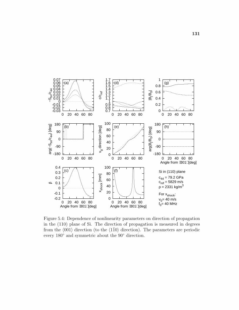
131
-0.03-0.02-0.01
0 0.01 0.02 0.03 0.04 0.05 0.06 0.07
0 20 40 60 80
−Slm
/c44
(a)
-180
-90
0
90
180
0 20 40 60 80
arg(
−Slm
/c44
) [d
eg]
(b)
-0.2 -0.1 0
0.1 0.2 0.3 0.4
0 20 40 60 80
β
(c)
Angle from ⟨001⟩ [deg]
0.7 0.8 0.9 1 1.1 1.2 1.3 1.4 1.5 1.6 1.7
0 20 40 60 80
c/c r
ef
(d)
0
20
40
60
80
100
0 20 40 60 80
v g d
irect
ion
[deg
] (e)
0
20
40
60
80
100
0 20 40 60 80
x sho
ck [m
m]
(f)
Angle from ⟨001⟩ [deg]
0
0.2
0.4
0.6
0.8
1
0 20 40 60 80
|Bj/B
0|
(g)
-180
-90
0
90
180
0 20 40 60 80
arg(
Bj/B
0) [d
eg] (h)
Angle from ⟨001⟩ [deg]
Si in (110) plane
c44 = 79.2 GPacref = 5829 m/sρ = 2331 kg/m3
For xshock:v0= 40 m/sf0= 40 MHz
Figure 5.4: Dependence of nonlinearity parameters on direction of propagationin the (110) plane of Si. The direction of propagation is measured in degreesfrom the 〈001〉 direction (to the 〈110〉 direction). The parameters are periodicevery 180◦ and symmetric about the 90◦ direction.
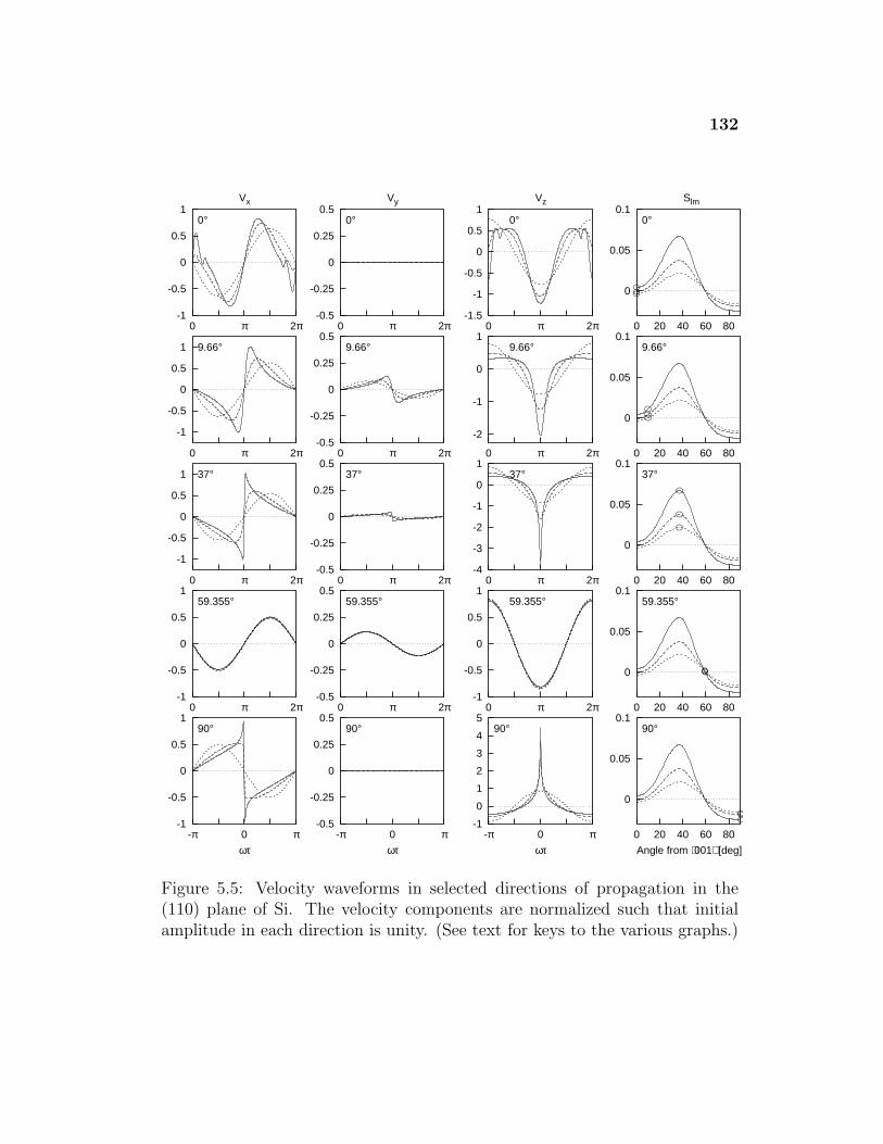
132
-1
-0.5
0
0.5
1
0 π 2π
0°
Vx
-0.5
-0.25
0
0.25
0.5
0 π 2π
0°
Vy
-1.5
-1
-0.5
0
0.5
1
0 π 2π
0°
Vz
0
0.05
0.1
0 20 40 60 80
Slm
0°
-1
-0.5
0
0.5
1
0 π 2π
9.66°
-0.5
-0.25
0
0.25
0.5
0 π 2π
9.66°
-2
-1
0
1
0 π 2π
9.66°
0
0.05
0.1
0 20 40 60 80
9.66°
-1
-0.5
0
0.5
1
0 π 2π
37°
-0.5
-0.25
0
0.25
0.5
0 π 2π
37°
-4
-3
-2
-1
0
1
0 π 2π
37°
0
0.05
0.1
0 20 40 60 80
37°
-1
-0.5
0
0.5
1
0 π 2π
59.355°
-0.5
-0.25
0
0.25
0.5
0 π 2π
59.355°
-1
-0.5
0
0.5
1
0 π 2π
59.355°
0
0.05
0.1
0 20 40 60 80
59.355°
-1
-0.5
0
0.5
1
-π 0 π
90°
ωτ
-0.5
-0.25
0
0.25
0.5
-π 0 π
90°
ωτ
-1
0
1
2
3
4
5
-π 0 π
90°
ωτ
0
0.05
0.1
0 20 40 60 80
90°
Angle from ⟨001⟩ [deg]
Nor
mal
ized
Vel
ocity
Wav
efor
ms
in (
110)
Pla
ne fo
r S
i
Figure 5.5: Velocity waveforms in selected directions of propagation in the(110) plane of Si. The velocity components are normalized such that initialamplitude in each direction is unity. (See text for keys to the various graphs.)
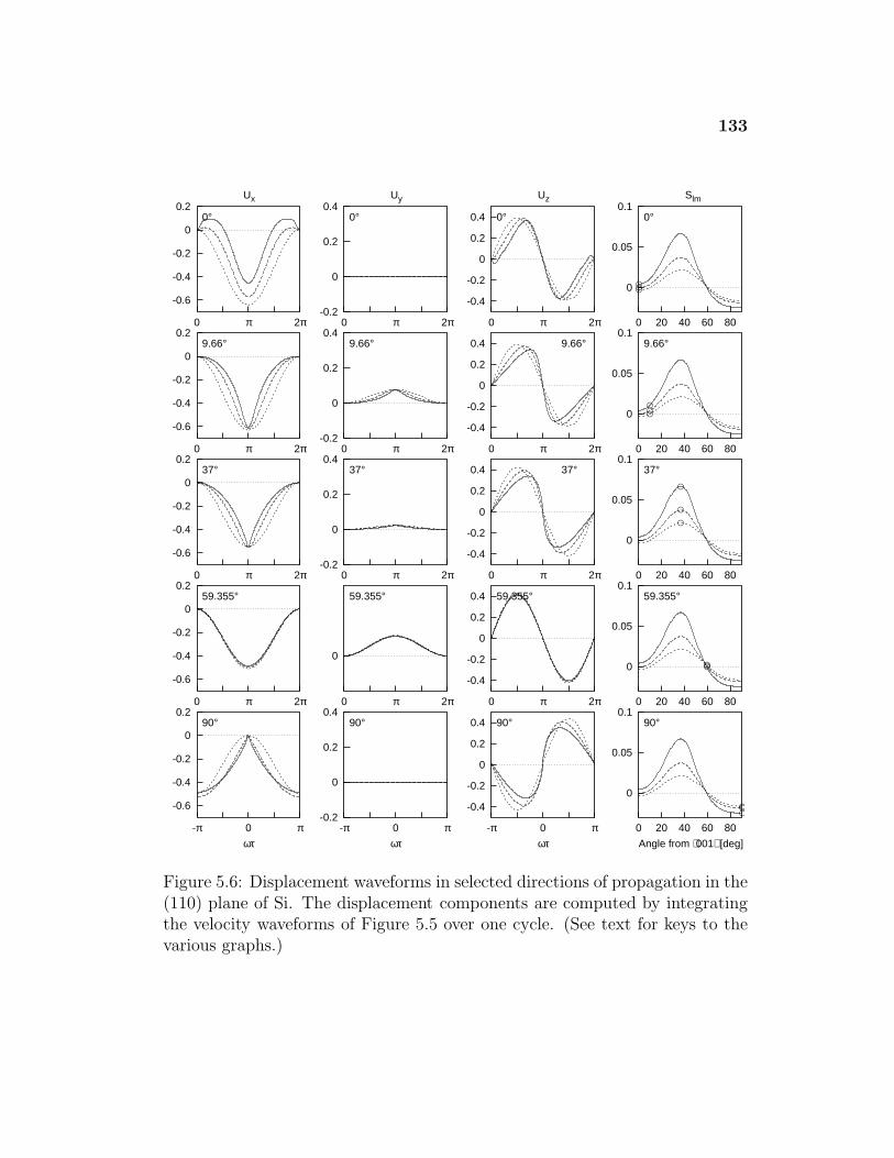
133
-0.6
-0.4
-0.2
0
0.2
0 π 2π
0°
Ux
-0.2
0
0.2
0.4
0 π 2π
0°
Uy
-0.4
-0.2
0
0.2
0.4
0 π 2π
0°
Uz
0
0.05
0.1
0 20 40 60 80
Slm
0°
-0.6
-0.4
-0.2
0
0.2
0 π 2π
9.66°
-0.2
0
0.2
0.4
0 π 2π
9.66°
-0.4
-0.2
0
0.2
0.4
0 π 2π
9.66°
0
0.05
0.1
0 20 40 60 80
9.66°
-0.6
-0.4
-0.2
0
0.2
0 π 2π
37°
-0.2
0
0.2
0.4
0 π 2π
37°
-0.4
-0.2
0
0.2
0.4
0 π 2π
37°
0
0.05
0.1
0 20 40 60 80
37°
-0.6
-0.4
-0.2
0
0.2
0 π 2π
59.355°
0
0 π 2π
59.355°
-0.4
-0.2
0
0.2
0.4
0 π 2π
59.355°
0
0.05
0.1
0 20 40 60 80
59.355°
-0.6
-0.4
-0.2
0
0.2
-π 0 π
90°
ωτ
-0.2
0
0.2
0.4
-π 0 π
90°
ωτ
-0.4
-0.2
0
0.2
0.4
-π 0 π
90°
ωτ
0
0.05
0.1
0 20 40 60 80
90°
Angle from ⟨001⟩ [deg]
Nor
mal
ized
Dis
plac
emen
t Wav
efor
ms
in (
110)
Pla
ne fo
r S
i
Figure 5.6: Displacement waveforms in selected directions of propagation in the(110) plane of Si. The displacement components are computed by integratingthe velocity waveforms of Figure 5.5 over one cycle. (See text for keys to thevarious graphs.)
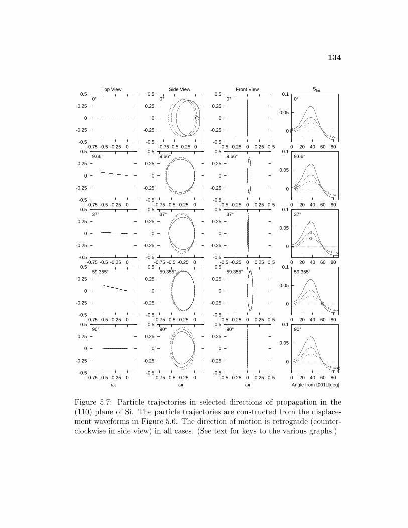
134
-0.5
-0.25
0
0.25
0.5
-0.75 -0.5 -0.25 0
0°
Top View
-0.5
-0.25
0
0.25
0.5
-0.75 -0.5 -0.25 0
0°
Side View
-0.5
-0.25
0
0.25
0.5
-0.5 -0.25 0 0.25 0.5
0°
Front View
0
0.05
0.1
0 20 40 60 80
Slm
0°
-0.5
-0.25
0
0.25
0.5
-0.75 -0.5 -0.25 0
9.66°
-0.5
-0.25
0
0.25
0.5
-0.75 -0.5 -0.25 0
9.66°
-0.5
-0.25
0
0.25
0.5
-0.5 -0.25 0 0.25 0.5
9.66°
0
0.05
0.1
0 20 40 60 80
9.66°
-0.5
-0.25
0
0.25
0.5
-0.75 -0.5 -0.25 0
37°
-0.5
-0.25
0
0.25
0.5
-0.75 -0.5 -0.25 0
37°
-0.5
-0.25
0
0.25
0.5
-0.5 -0.25 0 0.25 0.5
37°
0
0.05
0.1
0 20 40 60 80
37°
-0.5
-0.25
0
0.25
0.5
-0.75 -0.5 -0.25 0
59.355°
-0.5
-0.25
0
0.25
0.5
-0.75 -0.5 -0.25 0
59.355°
-0.5
-0.25
0
0.25
0.5
-0.5 -0.25 0 0.25 0.5
59.355°
0
0.05
0.1
0 20 40 60 80
59.355°
-0.5
-0.25
0
0.25
0.5
-0.75 -0.5 -0.25 0
90°
ωτ
-0.5
-0.25
0
0.25
0.5
-0.75 -0.5 -0.25 0
90°
ωτ
-0.5
-0.25
0
0.25
0.5
-0.5 -0.25 0 0.25 0.5
90°
ωτ
0
0.05
0.1
0 20 40 60 80
90°
Angle from ⟨001⟩ [deg]
Nor
mal
ized
Par
ticle
Tra
ject
orie
s in
(11
0) P
lane
for
Si
Figure 5.7: Particle trajectories in selected directions of propagation in the(110) plane of Si. The particle trajectories are constructed from the displace-ment waveforms in Figure 5.6. The direction of motion is retrograde (counter-clockwise in side view) in all cases. (See text for keys to the various graphs.)
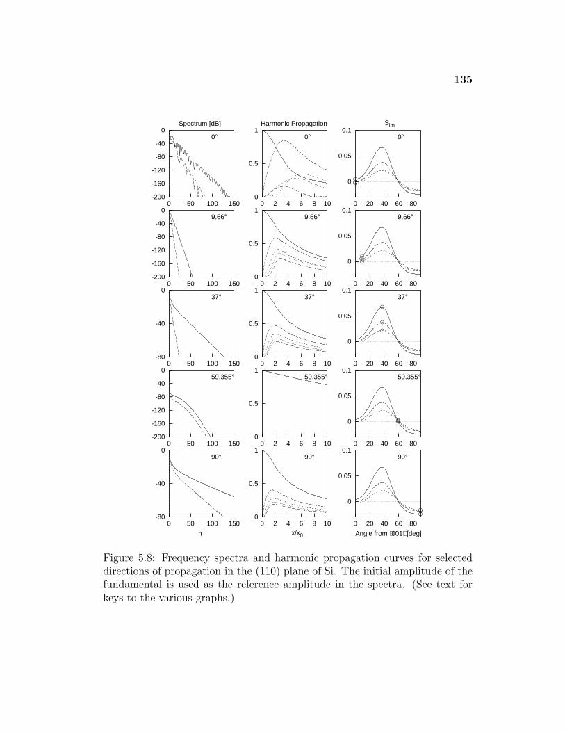
135
-200
-160
-120
-80
-40
0
0 50 100 150
0°
Spectrum [dB]
0
0.5
1
0 2 4 6 8 10
0°
Harmonic Propagation
0
0.05
0.1
0 20 40 60 80
Slm
0°
-200
-160
-120
-80
-40
0
0 50 100 150
9.66°
0
0.5
1
0 2 4 6 8 10
9.66°
0
0.05
0.1
0 20 40 60 80
9.66°
-80
-40
0
0 50 100 150
37°
0
0.5
1
0 2 4 6 8 10
37°
0
0.05
0.1
0 20 40 60 80
37°
-200
-160
-120
-80
-40
0
0 50 100 150
59.355°
0
0.5
1
0 2 4 6 8 10
59.355°
0
0.05
0.1
0 20 40 60 80
59.355°
-80
-40
0
0 50 100 150
90°
n
0
0.5
1
0 2 4 6 8 10
90°
x/x0
0
0.05
0.1
0 20 40 60 80
90°
Angle from ⟨001⟩ [deg]
Spe
ctra
and
Har
mon
ic P
ropa
gatio
n C
urve
s in
(11
0) P
lane
for
Si
Figure 5.8: Frequency spectra and harmonic propagation curves for selecteddirections of propagation in the (110) plane of Si. The initial amplitude of thefundamental is used as the reference amplitude in the spectra. (See text forkeys to the various graphs.)
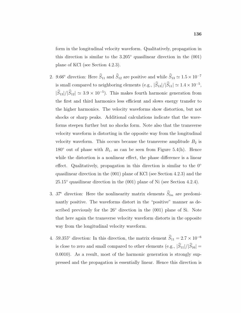
136
form in the longitudinal velocity waveform. Qualitatively, propagation in
this direction is similar to the 3.205◦ quasilinear direction in the (001)
plane of KCl (see Section 4.2.3).
2. 9.66◦ direction: Here S11 and S12 are positive and while S13 ' 1.5× 10⁻⁷
is small compared to neighboring elements (e.g., |S13|/|S11| ' 1.4× 10⁻⁵,
|S13|/|S12| ' 3.9 × 10⁻⁵). This makes fourth harmonic generation from
the first and third harmonics less efficient and slows energy transfer to
the higher harmonics. The velocity waveforms show distortion, but not
shocks or sharp peaks. Additional calculations indicate that the wave-
forms steepen further but no shocks form. Note also that the transverse
velocity waveform is distorting in the opposite way from the longitudinal
velocity waveform. This occurs because the transverse amplitude B2 is
180◦ out of phase with B1, as can be seen from Figure 5.4(h). Hence
while the distortion is a nonlinear effect, the phase difference is a linear
effect. Qualitatively, propagation in this direction is similar to the 0◦
quasilinear direction in the (001) plane of KCl (see Section 4.2.3) and the
25.15◦ quasilinear direction in the (001) plane of Ni (see Section 4.2.4).
3. 37◦ direction: Here the nonlinearity matrix elements Slm are predomi-
nantly positive. The waveforms distort in the “positive” manner as de-
scribed previously for the 26◦ direction in the (001) plane of Si. Note
that here again the transverse velocity waveform distorts in the opposite
way from the longitudinal velocity waveform.
4. 59.355◦ direction: In this direction, the matrix element S11 = 2.7× 10⁻⁶
is close to zero and small compared to other elements (e.g., |S11|/|S16| =0.0010). As a result, most of the harmonic generation is strongly sup-
pressed and the propagation is essentially linear. Hence this direction is
137
similar to the 20.785◦ and 32.315◦ quasilinear directions in the (001) plane
of Si. In this particular case, the element S16 was chosen to construct the
characteristic length scale x0 = x16 = ρc4/4|S16|ωv0. With v0 = 40 m/s
and f0 = 40 MHz, x0 = x16 ' 135 mm (as compared to the estimate
x11 ' 130000 mm).
5. 90◦ direction: Here the nonlinearity matrix elements Slm are predomi-
nantly negative, and waveforms distort in the “negative” manner as de-
scribed previously for the 0◦ and 35◦ directions in the (001) plane of Si.
Note that the horizontal scale on the waveform graphs has been shifted
by −π radians for this direction relative to the other directions.
In summary, the types of nonlinear waveform distortion seen in Si for this cut
are similar in many ways to the types of distortion seen in the (001) cut.
5.2.3 Study of KCl
Figure 5.9 shows the linear and nonlinear parameters of KCl in the (110) plane.
Figures 5.10 and 5.11 show the velocity waveforms and the frequency spectra
plus harmonic propagation curves, respectively. Figure 5.9(a) shows that S11,
S12, and S13 start out negative at 0◦, pass through zero around 10◦, and grow
to a local maximum around 45◦. They decrease to a local minimum around
71◦ and then abruptly rise to a global maximum around 74.5◦ before going to
zero at 90◦. The rapid changes in the matrix elements in the 70◦ to 90◦ range
are coincident with the convergence of the SAW mode with a transverse bulk
mode. This degeneration into an exceptional bulk wave at 90◦ can be seen
in both Figures 5.9(d) and (g). The standard deviation divided by the mean
for |S11|, |S12|, |S13| ranges between 70%–95% over the angular range shown.
In contrast, the standard deviation divided by the mean for the linear wave
138
-0.05 0
0.05 0.1
0.15 0.2
0.25 0.3
0.35 0.4
0.45
0 20 40 60 80
−Slm
/c44
(a)
-180
-90
0
90
180
0 20 40 60 80
arg(
−Slm
/c44
) [d
eg]
(b)
-0.2 0
0.2 0.4 0.6 0.8 1
1.2 1.4
0 20 40 60 80
β
(c)
Angle from ⟨001⟩ [deg]
0.8 1
1.2 1.4 1.6 1.8 2
2.2 2.4 2.6
0 20 40 60 80
c/c r
ef
(d)
0
20
40
60
80
100
0 20 40 60 80
v g d
irect
ion
[deg
] (e)
0
2
4
6
8
10
0 20 40 60 80
x sho
ck [m
m]
(f)
Angle from ⟨001⟩ [deg]
0
0.2
0.4
0.6
0.8
1
0 20 40 60 80
|Bj/B
0|
(g)
-180
-90
0
90
180
0 20 40 60 80
arg(
Bj/B
0) [d
eg] (h)
Angle from ⟨001⟩ [deg]
KCl in (110) plane
c44 = 6.3 GPacref = 1775 m/sρ = 1989 kg/m3
For xshock:v0= 40 m/sf0= 40 MHz
Figure 5.9: Dependence of nonlinearity parameters on direction of propagationin the (110) plane of KCl. The direction of propagation is measured in degreesfrom the 〈001〉 direction (to the 〈110〉 direction). The parameters are periodicevery 180◦ and symmetric about the 90◦ direction.
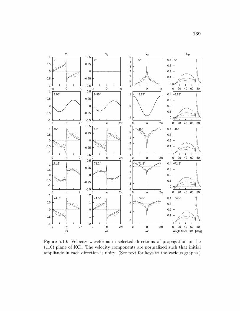
139
-1
-0.5
0
0.5
1
-π 0 π
0°
Vx
-0.5
-0.25
0
0.25
0.5
-π 0 π
0°
Vy
-1
0
1
2
3
4
5
-π 0 π
0°
Vz
0
0.1
0.2
0.3
0.4
0 20 40 60 80
Slm
0°
-1
-0.5
0
0.5
1
0 π 2π
9.95°
-0.5
-0.25
0
0.25
0.5
0 π 2π
9.95°
-1
0
1
0 π 2π
9.95°
0
0.1
0.2
0.3
0.4
0 20 40 60 80
9.95°
-1
-0.5
0
0.5
1
0 π 2π
45°
-0.5
-0.25
0
0.25
0.5
0 π 2π
45°
-4
-3
-2
-1
0
1
0 π 2π
45°
0
0.1
0.2
0.3
0.4
0 20 40 60 80
45°
-1
-0.5
0
0.5
1
0 π 2π
71.2°
-0.5
-0.25
0
0.25
0.5
0 π 2π
71.2°
-4
-3
-2
-1
0
1
0 π 2π
71.2°
0
0.1
0.2
0.3
0.4
0 20 40 60 80
71.2°
-1
-0.5
0
0.5
1
0 π 2π
74.5°
ωτ
-2
-1
0
1
2
0 π 2π
74.5°
ωτ
-2
-1
0
1
0 π 2π
74.5°
ωτ
0
0.1
0.2
0.3
0.4
0 20 40 60 80
74.5°
Angle from ⟨001⟩ [deg]
Nor
mal
ized
Vel
ocity
Wav
efor
ms
in (
110)
Pla
ne fo
r K
Cl
Figure 5.10: Velocity waveforms in selected directions of propagation in the(110) plane of KCl. The velocity components are normalized such that initialamplitude in each direction is unity. (See text for keys to the various graphs.)
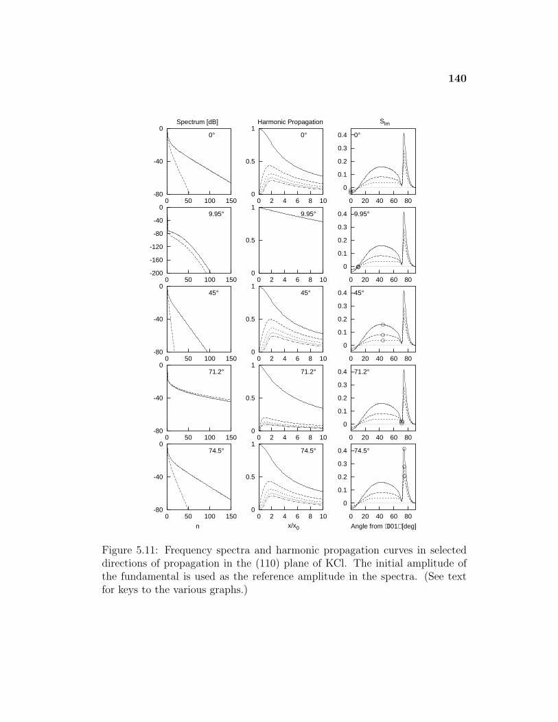
140
-80
-40
0
0 50 100 150
0°
Spectrum [dB]
0
0.5
1
0 2 4 6 8 10
0°
Harmonic Propagation
0
0.1
0.2
0.3
0.4
0 20 40 60 80
Slm
0°
-200
-160
-120
-80
-40
0
0 50 100 150
9.95°
0
0.5
1
0 2 4 6 8 10
9.95°
0
0.1
0.2
0.3
0.4
0 20 40 60 80
9.95°
-80
-40
0
0 50 100 150
45°
0
0.5
1
0 2 4 6 8 10
45°
0
0.1
0.2
0.3
0.4
0 20 40 60 80
45°
-80
-40
0
0 50 100 150
71.2°
0
0.5
1
0 2 4 6 8 10
71.2°
0
0.1
0.2
0.3
0.4
0 20 40 60 80
71.2°
-80
-40
0
0 50 100 150
74.5°
n
0
0.5
1
0 2 4 6 8 10
74.5°
x/x0
0
0.1
0.2
0.3
0.4
0 20 40 60 80
74.5°
Angle from ⟨001⟩ [deg]
Spe
ctra
and
Har
mon
ic P
ropa
gatio
n C
urve
s in
(11
0) P
lane
for
KC
l
Figure 5.11: Frequency spectra and harmonic propagation curves in selecteddirections of propagation in the (110) plane of KCl. The initial amplitude ofthe fundamental is used as the reference amplitude in the spectra. (See textfor keys to the various graphs.)
141
speed is around 6% (see Figure 5.9(d)). As above, the estimates of the shock
formation distances given in Figure 5.9(f) are probably inaccurate near quasi-
linear directions or directions where the amplitude of |S11| is small compared
to neighboring elements.
Several directions are selected for consideration in detail:
1. 0◦ direction: In this direction, the nonlinearity matrix elements Slm are
predominantly negative, and the waveform distorts in the characteristi-
cally “negative” manner. Note that the horizontal scale on the waveform
graphs has been shifted by −π radians for this direction relative to the
other directions in the figure.
2. 9.95◦ direction: Here the matrix element S11 = −4.8 × 10⁻⁶ is close to
zero and small compared to other elements (e.g., |S11|/|S15| = 0.0011).
Hence second harmonic generation is suppressed and the propagation is
essentially linear. In this particular case, the element S15 was chosen to
construct the characteristic length scale x0 = x15 = ρc4/4|S15|ωv0. With
v0 = 40 m/s and f0 = 40 MHz, x0 = x15 ' 16 mm (as compared to the
estimate x11 ' 15000 mm).
3. 45◦ direction: In this direction, the matrix elements Slm are predomi-
nantly positive, and the waveform distorts in the characteristically “pos-
itive” manner.
4. 71.2◦ direction: Here the matrix element S11 ' 9.5× 10⁻³ is small com-
pared to some of the other directions, but still nonzero. However, this
direction is a case where |S11| is less than neighboring elements (e.g.,
|S11|/|S12| ' 0.48, |S11|/|S13| ' 0.38), similar to the 10◦ and 45◦ direc-
tions in the (001) cut of KCl. The larger relative magnitudes of S12 and
S13 result in the transfer of energy to higher harmonics at a rapid rate,
142
and leads to the sharper cusps seen in the waveforms for this direction.
This direction is very close to a pure mode and hence may be favorable
for experimental investigation.
5. 74.5◦ direction: Here the matrix elements are predominantly positive,
and the waveform distorts in the characteristically “positive” manner.
In conclusion, the discussion above shows that the types of waveform distortion
seen in this cut are similar to those in the (110) cut of Si and the materials in
the (001) case.
5.2.4 Study of Ni
Figure 5.12 shows the linear and nonlinear parameters of Ni in the (110) plane.
For several selected directions, Figure 5.13 shows the velocity waveforms, and
Figure 5.14 displays the frequency spectra and harmonic propagation curves.
Figure 5.12(a) indicates that S11, S12, and S13 are positive over almost the
whole range, with a global maximum at 0◦ and a local maximum around 55.5◦.
Near 90◦, |S11| becomes very small and the other elements become negative but
still relatively small in magnitude. The standard deviation divided by the mean
for |S11|, |S12|, |S13| ranges between 55%–65% over the angular range shown.
In contrast, the standard deviation divided by the mean for the linear wave
speed is around 8% [see Figure 5.12(d)]. This proportionally larger variation is
consistent with other materials in the (110) plane.
In all these directions except 90◦, the matrix elements Slm are predom-
inantly positive, and the waveforms distort in the characteristically “positive”
manner. A few additional comments are provided for the directions shown in
the figures:
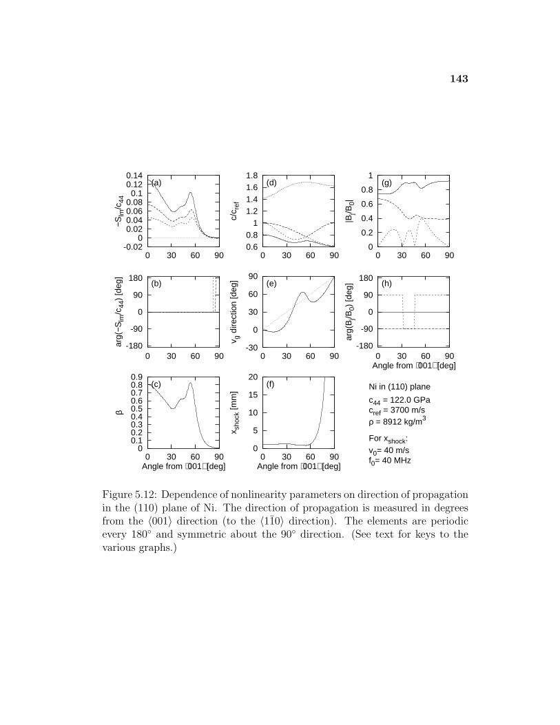
143
-0.02 0
0.02 0.04 0.06 0.08 0.1
0.12 0.14
0 30 60 90
−Slm
/c44
(a)
-180
-90
0
90
180
0 30 60 90
arg(
−Slm
/c44
) [d
eg]
(b)
0 0.1 0.2 0.3 0.4 0.5 0.6 0.7 0.8 0.9
0 30 60 90
β
(c)
Angle from ⟨001⟩ [deg]
0.6 0.8 1
1.2 1.4 1.6 1.8
0 30 60 90
c/c r
ef
(d)
-30
0
30
60
90
0 30 60 90
v g d
irect
ion
[deg
] (e)
0
5
10
15
20
0 30 60 90
x sho
ck [m
m]
(f)
Angle from ⟨001⟩ [deg]
0
0.2
0.4
0.6
0.8
1
0 30 60 90
|Bj/B
0|
(g)
-180
-90
0
90
180
0 30 60 90ar
g(B
j/B0)
[deg
] (h)
Angle from ⟨001⟩ [deg]
Ni in (110) plane
c44 = 122.0 GPacref = 3700 m/sρ = 8912 kg/m3
For xshock:v0= 40 m/sf0= 40 MHz
Figure 5.12: Dependence of nonlinearity parameters on direction of propagationin the (110) plane of Ni. The direction of propagation is measured in degreesfrom the 〈001〉 direction (to the 〈110〉 direction). The elements are periodicevery 180◦ and symmetric about the 90◦ direction. (See text for keys to thevarious graphs.)
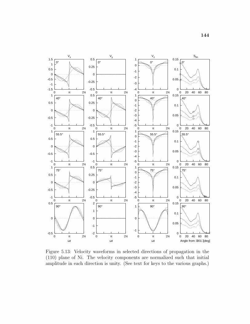
144
-1.5
-1
-0.5
0
0.5
1
1.5
0 π 2π
0°
Vx
-0.5
-0.25
0
0.25
0.5
0 π 2π
0°
Vy
-4
-3
-2
-1
0
1
0 π 2π
0°
Vz
0
0.05
0.1
0.15
0 20 40 60 80
Slm
0°
-1
-0.5
0
0.5
1
0 π 2π
40°
-0.5
-0.25
0
0.25
0.5
0 π 2π
40°
-5
-4
-3
-2
-1
0
1
0 π 2π
40°
0
0.05
0.1
0.15
0 20 40 60 80
40°
-1
-0.5
0
0.5
1
0 π 2π
55.5°
-1
-0.5
0
0.5
1
0 π 2π
55.5°
-5
-4
-3
-2
-1
0
1
0 π 2π
55.5°
0
0.05
0.1
0.15
0 20 40 60 80
55.5°
-1
-0.5
0
0.5
1
0 π 2π
75°
-0.5
-0.25
0
0.25
0.5
0 π 2π
75°
-5
-4
-3
-2
-1
0
1
0 π 2π
75°
0
0.05
0.1
0.15
0 20 40 60 80
75°
-0.5
0
0.5
0 π 2π
90°
ωτ
-2
-1
0
1
2
0 π 2π
90°
ωτ
-1
0
1
0 π 2π
90°
ωτ
0
0.05
0.1
0.15
0 20 40 60 80
90°
Angle from ⟨001⟩ [deg]
Nor
mal
ized
Vel
ocity
Wav
efor
ms
in (
110)
Pla
ne fo
r N
i
Figure 5.13: Velocity waveforms in selected directions of propagation in the(110) plane of Ni. The velocity components are normalized such that initialamplitude in each direction is unity. (See text for keys to the various graphs.)
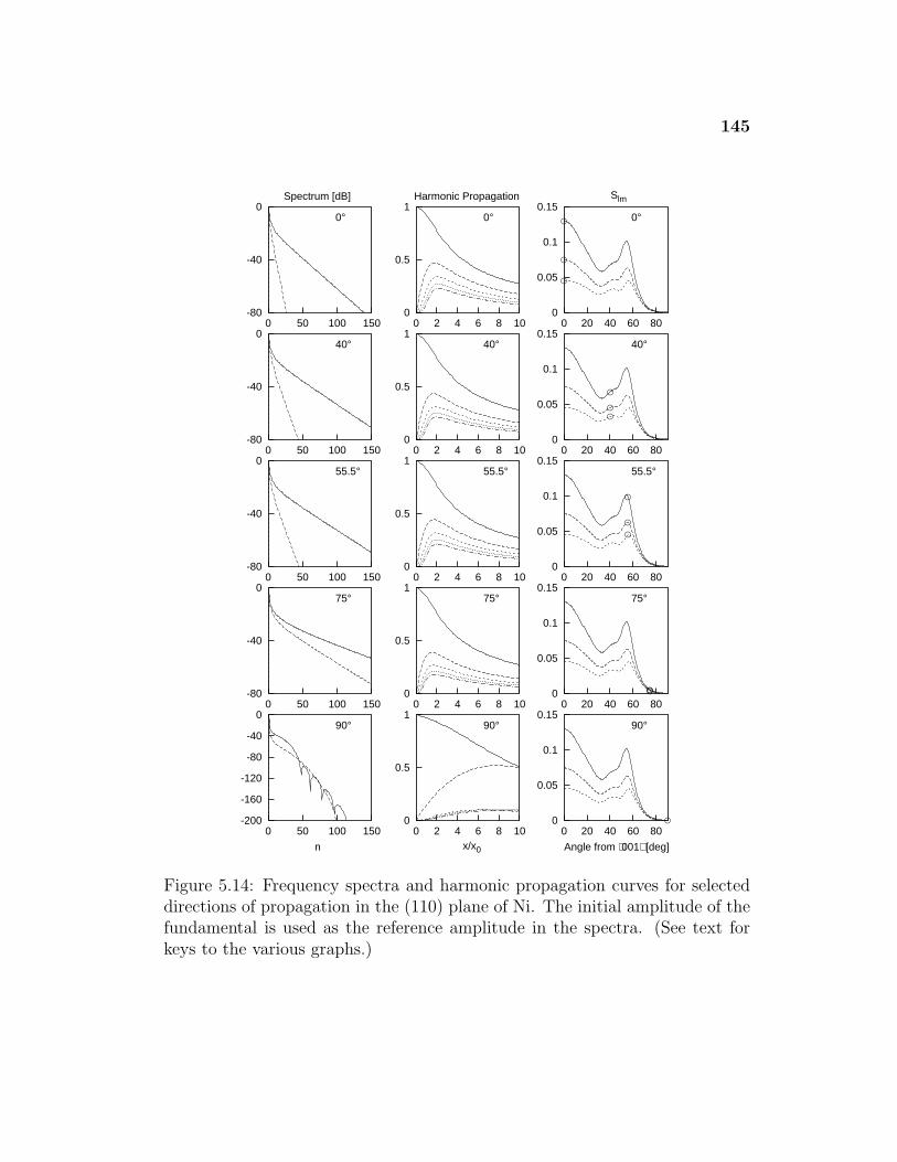
145
-80
-40
0
0 50 100 150
0°
Spectrum [dB]
0
0.5
1
0 2 4 6 8 10
0°
Harmonic Propagation
0
0.05
0.1
0.15
0 20 40 60 80
Slm
0°
-80
-40
0
0 50 100 150
40°
0
0.5
1
0 2 4 6 8 10
40°
0
0.05
0.1
0.15
0 20 40 60 80
40°
-80
-40
0
0 50 100 150
55.5°
0
0.5
1
0 2 4 6 8 10
55.5°
0
0.05
0.1
0.15
0 20 40 60 80
55.5°
-80
-40
0
0 50 100 150
75°
0
0.5
1
0 2 4 6 8 10
75°
0
0.05
0.1
0.15
0 20 40 60 80
75°
-200
-160
-120
-80
-40
0
0 50 100 150
90°
n
0
0.5
1
0 2 4 6 8 10
90°
x/x0
0
0.05
0.1
0.15
0 20 40 60 80
90°
Angle from ⟨001⟩ [deg]
Spe
ctra
and
Har
mon
ic P
ropa
gatio
n C
urve
s in
(11
0) P
lane
for
Ni
Figure 5.14: Frequency spectra and harmonic propagation curves for selecteddirections of propagation in the (110) plane of Ni. The initial amplitude of thefundamental is used as the reference amplitude in the spectra. (See text forkeys to the various graphs.)
146
1. 0◦ direction: The wave is of the “Rayleigh-type” in this direction. Its
distortion is then similar to the 0◦ direction in KCl but occurs in the
opposite manner.
2. 40◦ direction: This direction was selected because it is a pure mode, and
hence conducive to experimental investigation. The transverse compo-
nent B2 is nonzero and in phase with B1.
3. 55.5◦ direction: Like the 40◦ direction, the 55.5◦ direction is also a pure
mode direction, and the transverse component B2 is nonzero. However,
the distortion in the transverse velocity waveform is in the opposite di-
rection of the longitudinal velocity. This occurs because B1 and B2 are
180◦ out of phase in this angular region [See Figure 5.12(g)].
4. 75◦ direction: In this region, the nonlinearity is around an order of magni-
tude less than the 0◦ direction. While the waveforms form shocks, they do
so over considerably large distances. The spectrum in Figure 5.13. shows
more energy in the higher harmonics at X = 1 than in previous directions,
correspondingly, the waveforms appear to show a slightly sharper cusps in
Figure 5.14. Additional calculations show that this is caused by increased
relative magnitudes of |S12|/|S11| = 0.80 and |S13|/|S11| = 0.75 in this di-
rection. In contrast, the more typical 55.5◦ case has |S12|/|S11| = 0.62
and |S13|/|S11| = 0.44. This case is a similar but weaker version of the
type of propagation in 71.2◦ direction in the (110) plane of KCl.
5. 90◦ direction: Here S11 = 4.7 × 10⁻⁴ is positive but close to zero and
somewhat smaller than neighboring elements (e.g., |S11|/|S1,10| = 0.31).
Higher order elements are predominantly negative. The resulting wave-
form distortion is close to linear but with a slight “negative” trend. For
147
this particular case, the element S1,10 was chosen to construct the char-
acteristic length scale x0 = x1,10 = ρc4/4|S1,10|ωv0 = 32 mm used in the
figures (as compared with the estimate x11 ' 100 mm).
Thus, nonlinear SAWs in the (110) plane of Ni display many of the same
properties as other nonlinear SAWs in the (110) and (001) planes.
5.3 Summary
This chapter has investigated the properties of nonlinear SAWs in the (110)
plane of a variety of cubic crystals. The types of propagation seen in materials
in the m3m point group in this cut are very similar to those seen in the (001)
plane. The largest difference occurs in materials in the m3 point group (alums),
for which the matrix elements become complex-valued. Investigation of the
meaning of complex-valued nonlinearity is the main theme of Chapter 6.
Chapter 6
Monofrequency SAWs in the (111) Plane
This chapter discusses nonlinear propagation of monofrequency SAWs in the
(111) plane of selected cubic crystals. (See Figure D.1 for a diagram of this
cut.) Because the (111) plane is not a plane of high symmetry, the nonlinearity
matrix elements are generally complex-valued and the waveform distortion is
significantly more complicated. Nevertheless, the plots of the magnitude and
phase of the nonlinearity matrix elements as a function of direction can still
be used to indicate waveform distortion properties. The chapter begins with a
brief overview of linear properties and a general review of nonlinear effects in
a variety of crystals. Next, an interpretation of the phase of the nonlinearity
matrix elements is proposed based on a simple mathematical transformation.
Last, detailed studies of Si, KCl, and Ni are presented and discussed.
6.1 Linear Effects
The SAW speed of selected materials as a function of the propagation direction
is shown in Figure 6.1. The direction of propagation is measured in degrees
from the 〈112〉 direction,∗ and the speed for each material is scaled by the
characteristic speed cref = (c44/ρ)1/2 for that material. Because the normal to
the (111) plane is a sixfold symmetry axis, the SAW speed is periodic every
∗Note that Farnell3 chooses the reference direction to be 〈110〉. Hence his plots of thewave speed are reversed as compared to Figure 6.1 (i.e., directions cited as θ degrees hereare given there as 30◦ − θ).
148
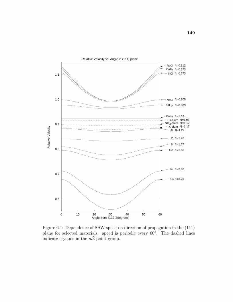
149
0.6
0.7
0.8
0.9
1.0
1.1
0 10 20 30 40 50 60
Rel
ativ
e V
eloc
ity
Angle from ⟨112⟩ [degrees]
Relative Velocity vs. Angle in (111) plane
η=0.312RbClCaF2 η=0.373
η=0.373KCl
NaCl η=0.705
SrF 2 η=0.803
η=1.02BaF2η=1.06Cs-alum
-alum4 η=1.12NHK-alum η=1.17
Al η=1.22
C η=1.26
Si η=1.57
Ge η=1.66
Ni η=2.60
Cu η=3.20
Figure 6.1: Dependence of SAW speed on direction of propagation in the (111)plane for selected materials. speed is periodic every 60◦. The dashed linesindicate crystals in the m3 point group.
150
60◦. Note that only the range from 0◦ to 30◦ is shown because the 30◦ direction
is normal to a plane of mirror symmetry. In most cases (for all the cases
shown here), the speeds group by anisotropy ratio, with materials with lower
anisotropy ratios having higher relative SAW speeds. Materials with η ≈ 1
indicate nearly isotropic media, with a correspondingly constant SAW speed
for all directions. Crystals in the m3 point group are plotted using dashed
lines.
6.2 Nonlinear Effects
This section demonstrates that SAWs in (111) plane have the following prop-
erties:
• Nonlinear SAWs for most directions in the (111) plane are described
by nonlinearity matrix elements which are complex-valued. Both the
magnitude and phase of the matrix elements can be related to the type
of waveform distortion.
• The waveforms generally exhibit asymmetric distortion. In some cases,
this causes the shock formation to be less clearly defined.
• A simple mathematical transformation is proposed to interpret the phase
information in the nonlinearity matrix elements in cases where the phase
of the lowest order matrix elements are the same.
• In cases where the phases of the nonlinearity matrix elements are not the
same, the waveforms exhibit a nonlinear dispersion-like effect in which
oscillations form near the shocks and peaks of the velocity waveforms.
As shown below, nonlinear SAWs in the (111) plane are often significantly
different from those in the (001) and (110) planes.
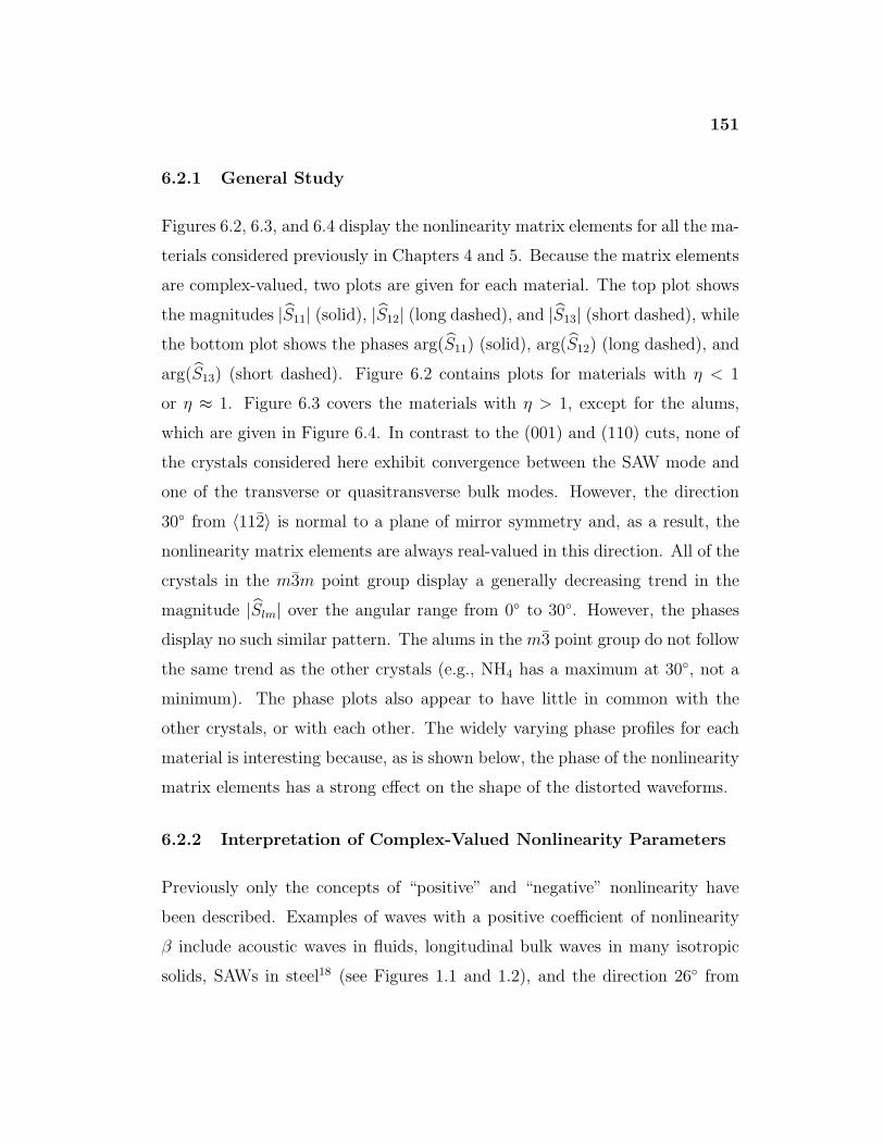
151
6.2.1 General Study
Figures 6.2, 6.3, and 6.4 display the nonlinearity matrix elements for all the ma-
terials considered previously in Chapters 4 and 5. Because the matrix elements
are complex-valued, two plots are given for each material. The top plot shows
the magnitudes |S11| (solid), |S12| (long dashed), and |S13| (short dashed), while
the bottom plot shows the phases arg(S11) (solid), arg(S12) (long dashed), and
arg(S13) (short dashed). Figure 6.2 contains plots for materials with η < 1
or η ≈ 1. Figure 6.3 covers the materials with η > 1, except for the alums,
which are given in Figure 6.4. In contrast to the (001) and (110) cuts, none of
the crystals considered here exhibit convergence between the SAW mode and
one of the transverse or quasitransverse bulk modes. However, the direction
30◦ from 〈112〉 is normal to a plane of mirror symmetry and, as a result, the
nonlinearity matrix elements are always real-valued in this direction. All of the
crystals in the m3m point group display a generally decreasing trend in the
magnitude |Slm| over the angular range from 0◦ to 30◦. However, the phases
display no such similar pattern. The alums in the m3 point group do not follow
the same trend as the other crystals (e.g., NH4 has a maximum at 30◦, not a
minimum). The phase plots also appear to have little in common with the
other crystals, or with each other. The widely varying phase profiles for each
material is interesting because, as is shown below, the phase of the nonlinearity
matrix elements has a strong effect on the shape of the distorted waveforms.
6.2.2 Interpretation of Complex-Valued Nonlinearity Parameters
Previously only the concepts of “positive” and “negative” nonlinearity have
been described. Examples of waves with a positive coefficient of nonlinearity
β include acoustic waves in fluids, longitudinal bulk waves in many isotropic
solids, SAWs in steel18 (see Figures 1.1 and 1.2), and the direction 26◦ from
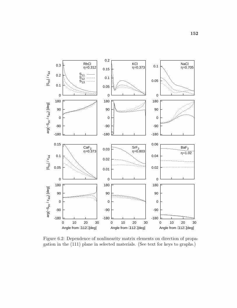
152
0
0.1
0.2
0.3
RbClη=0.312
S11S12S13
0
0.05
0.1
0.15
0.2
KClη=0.373
0
0.05
0.1
NaClη=0.705
-180
-90
0
90
180
-180
-90
0
90
180
-180
-90
0
90
180
0
0.05
0.1
0.15
CaF2η=0.373
0
0.01
0.02
0.03
SrF2η=0.803
0
0.02
0.04
0.06
BaF2
η=1.02
-180
-90
0
90
180
0 10 20 30
Angle from ⟨112⟩ [deg]
-180
-90
0
90
180
0 10 20 30
Angle from ⟨112⟩ [deg]
-180
-90
0
90
180
0 10 20 30
Angle from ⟨112⟩ [deg]
arg(
−Slm
/ c 4
4) [d
eg]
|Slm
| / c
44ar
g(−S
lm /
c 44)
[deg
] |S
lm| /
c44
Normalized Nonlinearity Matrix Elements in (111) Plane for Selected Materials
Figure 6.2: Dependence of nonlinearity matrix elements on direction of propa-gation in the (111) plane in selected materials. (See text for keys to graphs.)
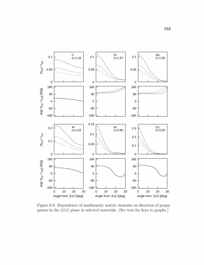
153
0
0.05
0.1
Cη=1.26
0
0.05
0.1
Siη=1.57
0
0.05
0.1
Geη=1.66
-180
-90
0
90
180
-180
-90
0
90
180
-180
-90
0
90
180
0
0.1
0.2
Alη=1.22
0
0.05
0.1
0.15
Niη=2.60
0
0.1
0.2
0.3
Cuη=3.20
-180
-90
0
90
180
0 10 20 30
Angle from ⟨112⟩ [deg]
-180
-90
0
90
180
0 10 20 30
Angle from ⟨112⟩ [deg]
-180
-90
0
90
180
0 10 20 30
Angle from ⟨112⟩ [deg]
arg(
−Slm
/ c 4
4) [d
eg]
|Slm
| / c
44ar
g(−S
lm /
c 44)
[deg
] |S
lm| /
c44
Normalized Nonlinearity Matrix Elements in (111) Plane for Selected Materials
Figure 6.3: Dependence of nonlinearity matrix elements on direction of propa-gation in the (111) plane in selected materials. (See text for keys to graphs.)
154
0
0.02
0.04
0.06
Cs-alum η=1.06
0
0.02
0.04
NH4-alumη=1.12
0
0.05
0.1
K-alumη=1.17
-180
-90
0
90
180
0 10 20 30
Angle from ⟨112⟩ [deg]
S11S12S13
-180
-90
0
90
180
0 10 20 30
Angle from ⟨112⟩ [deg]
-180
-90
0
90
180
0 10 20 30
Angle from ⟨112⟩ [deg]
arg(
−Slm
/ c 4
4) [d
eg]
|Slm
| / c
44
Normalized Nonlinearity Matrix Elements in (111) Plane for Selected Materials
Figure 6.4: Dependence of nonlinearity matrix elements on direction of propa-gation in the (111) plane in selected materials. (See text for keys to graphs.)
〈100〉 in Si. In these waves, the peaks of the waves advance in a retarded time
frame moving at the linear wave speed, while the troughs recede. Examples of
waves with β < 0 include SAWs in fused quartz26 and SAWs propagating in
the directions 0◦ and 35◦ from 〈100〉 in the (001) plane of Si (see Figure 4.5). In
these waves, the peaks of the wave recede in a retarded time frame moving at
the linear wave speed, while the the troughs advance. However, the situation is
more complicated for the most general case of a SAW in an anisotropic medium.
As shown in Section 2.2.2, the coefficient of nonlinearity for SAWs in crystal is
[Eq. (2.63) with Eq. (4.5)]
β =4c44S11
ρc2, (6.1)
where the nonlinearity matrix element S11 = |S11|eiφS can be complex-valued.
The interpretation of Eq. (6.1) in terms of its effect on waveforms for situations
155
other than φS = 0 (β real and positive) and φS = ±π (β real and negative)
is not immediately obvious. The purpose of this section is to suggest a way of
thinking about this issue.
Ideally, one would like to be able to characterize the type of waveform
distortion by computing just a few parameters, thereby avoiding the process of
numerically integrating a system of nonlinear differential equations for every
material, cut, and direction. As shown in Chapters 4 and 5, the nonlinearity
matrix elements serve as such parameters, allowing a reasonable estimate of
the type of waveform distortion (or lack thereof) to be determined from plots
of the first few elements. The ability to make the same type of estimate is
desired here. The specific objective is to investigate in a simple manner how
the phase of the nonlinearity matrix affects the SAW solutions.
Towards this end, the quantity
Sθlm = Slmeiθ (6.2)
is introduced to represent a nonlinearity matrix constructed by applying a
uniform phase increment θ to a given matrix Slm. Given a solution for a
material with matrix Slm, it is desired to relate that solution to the one obtained
for a material with nonlinearity matrix Sθlm. It is convenient, although not
necessary, to consider the matrix Slm to be real, as is typical for isotropic
solids. The main simplifying assumption here is that there exist materials for
which the phase of the nonlinearity matrix is nonzero yet independent of the
indices l and m. That Eq. (6.2) is a reasonable model of the phase dependence,
for at least the lowest several matrix elements, is supported by Figures 6.2–6.4.
However, in order for Eq. (6.2) to be valid, Sθlm must retain all the
symmetry properties required of the nonlinearity matrix. In particular, the
nonlinearity matrix elements have the symmetry property [Hamilton et al.,33
156
Eq. (80)]
Slm(−n) = S∗(−l)(−m)n , (6.3)
where n = l + m. By straightforward substitution, it is seen that Eq. (6.2)
holds only for n > 0. In contrast, if the definition
Sθlm = Slmei(n/|n|)θ (6.4)
is adopted in place of Eq. (6.2), then Eq. (6.4) holds for all n. Henceforth the
quantity Sθlm refers to the definition in Eq. (6.4).
Next, recall that the evolution equation for a material with nonlinearity
matrix Sθlm [Eq. (2.87)] is given by
dvθn
dx=
n2ω0
2ρc4
∑l+m=n
lm
|lm|Sθlm(−n)v
θl v
θm , (6.5)
where the notation vθn designates that these spectral components are the solu-
tions associated with the matrix Sθlm. Now substitute Eq. (6.4) into Eq. (6.5)
and multiply both sides by ei(n/|n|)θ, let
vn = vθne
i(n/|n|)θ , (6.6)
and rewrite Eq. (6.5) as
dvn
dx=
n2ω0
2ρc4
∑l+m=n
lm
|lm|Slm(−n)vlvm . (6.7)
The spectral components vn in Eq. (6.7) are recognized as the solutions for a
material with nonlinearity matrix Slm. Therefore, the solutions vθn for a material
with nonlinearity matrix Sθlm are related to the solutions vn for a material with
nonlinearity matrix Slm via Eq. (6.6):
vθn = vne
−i(n/|n|)θ . (6.8)
157
The velocity components vθj in the xj direction for a material with nonlinearity
matrix Sθlm are reconstructed from the spectral components vθ
n via Eq. (2.35):
vθj (x, z, τ) =
∞∑n=−∞
vθn(x)unj(z)e−inω0τ , (6.9)
where the depth functions uni are given by Eq. (2.13), τ = t − x/c, and ω0 is
the characteristic angular frequency. At the surface (z = 0), Eq. (6.9) reduces
to
vθj (x, τ) =
∞∑n=−∞
vθn(x)|Bj |ei(n/|n|)φBje−inω0τ , (6.10)
where the linear amplitude factors Bj are defined in Eq. (2.42). For ease of
notation in the remainder of the chapter, define
Sθlm = −Sθ
lm
c44, (6.11)
following the definition of Slm in Eq. (4.5).
As an example of this procedure, take the well-known waveform dis-
tortion for a “positively” distorting nonlinear Rayleigh wave as a reference
case, with reference spectra vRn and corresponding real-valued nonlinearity
matrix elements SRlm under the convention∗ that the linear amplitude factor
BR1 = |BR
1 |e−iπ/2 = −i|BR1 |. For simplicity, only consider the longitudinal ve-
locity waveforms (the other velocity components are considered near the end
of the section). The reference longitudinal velocity waveform for the nonlinear
Rayleigh wave is given by
vR1 (x, τ) =
∞∑n=−∞
vRn (x)
(−i
n
|n| |BR1 |)
e−inω0τ . (6.12)
∗This convention is chosen to be consistent with the nonlinear Rayleigh wave theory ofZabolotskaya.20 Here B1 is analogous to i(ξt + η), where ξt + η < 0 for all isotropic media(see Table 2.3 and Figure 2.5).
158
Suppose there exists a hypothetical crystal with nonlinearity matrix elements
Sθlm = SR
lmei(n/|n|)θ and linear amplitude factors B1 = |B1|e−iπ/2 = −i|B1|. By
Eq. (6.10), the longitudinal velocity waveform at the surface of the crystal is
written in terms of the spectral components of the reference Rayleigh wave as
vθ1(x, τ) =
∞∑n=−∞
vθn(x)
(−i
n
|n| |B1|)
e−inω0τ , (6.13)
or, using Eq. (6.8),
vθ1(x, τ) =
|B1||BR
1 |∞∑
n=−∞vR
n (x)e−i(n/|n|)θ(−i
n
|n| |BR1 |)
e−inω0τ . (6.14)
The summation is the longitudinal velocity waveform of the Rayleigh wave,
except for the factor of e−i(n/|n|)θ. The prefactor |B1|/|BR1 | adjusts for possible
amplitude differences between the linear solutions of the Rayleigh wave and
the SAW in the crystal. Thus, given the crystal’s linear amplitude factor B1
and the phase θ of the crystal’s nonlinearity matrix elements, the waveforms
at the surface in the idealized crystal may be computed by changing the phase
of the spectral components of the nonlinear Rayleigh wave and reconstructing
according to Eq. (6.14).
However, as shown below, the waveforms of real crystals computed from
the Rayleigh waveforms by Eq. (6.14) are not generally the same as the wave-
forms computed directly by integrating Eq. (6.7). Hence in most cases the
expression in Eq. (6.14) is only an approximation to the actual waveform. The
discrepancies occur because crystals rarely have all their nonlinearity matrix el-
ements with identical phase and, even if the phases of the elements are similar,
the magnitudes of the elements may differ. Nevertheless, the overall result can
be qualitatively similar, especially in cases where the dominant matrix elements
have close to the same phase.
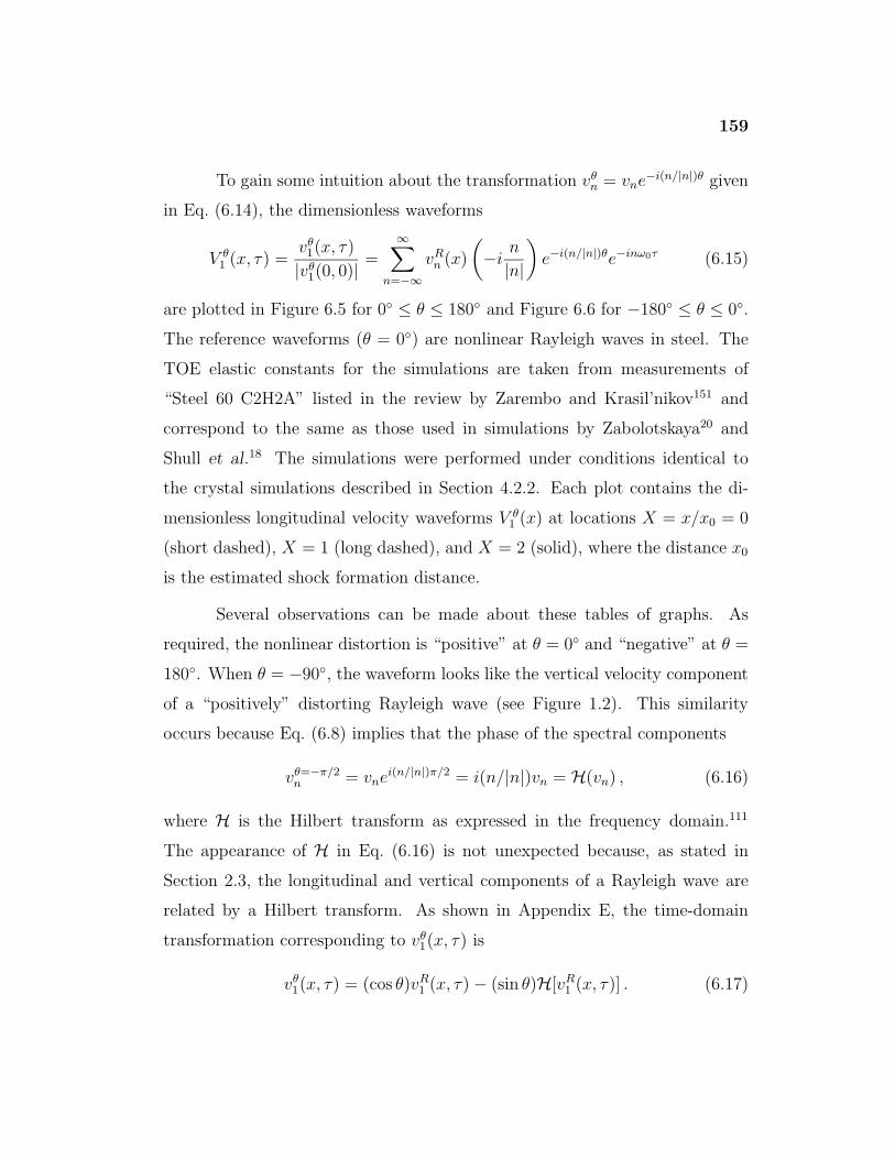
159
To gain some intuition about the transformation vθn = vne−i(n/|n|)θ given
in Eq. (6.14), the dimensionless waveforms
V θ1 (x, τ) =
vθ1(x, τ)
|vθ1(0, 0)| =
∞∑n=−∞
vRn (x)
(−i
n
|n|)
e−i(n/|n|)θe−inω0τ (6.15)
are plotted in Figure 6.5 for 0◦ ≤ θ ≤ 180◦ and Figure 6.6 for −180◦ ≤ θ ≤ 0◦.
The reference waveforms (θ = 0◦) are nonlinear Rayleigh waves in steel. The
TOE elastic constants for the simulations are taken from measurements of
“Steel 60 C2H2A” listed in the review by Zarembo and Krasil’nikov151 and
correspond to the same as those used in simulations by Zabolotskaya20 and
Shull et al.18 The simulations were performed under conditions identical to
the crystal simulations described in Section 4.2.2. Each plot contains the di-
mensionless longitudinal velocity waveforms V θ1 (x) at locations X = x/x0 = 0
(short dashed), X = 1 (long dashed), and X = 2 (solid), where the distance x0
is the estimated shock formation distance.
Several observations can be made about these tables of graphs. As
required, the nonlinear distortion is “positive” at θ = 0◦ and “negative” at θ =
180◦. When θ = −90◦, the waveform looks like the vertical velocity component
of a “positively” distorting Rayleigh wave (see Figure 1.2). This similarity
occurs because Eq. (6.8) implies that the phase of the spectral components
vθ=−π/2n = vnei(n/|n|)π/2 = i(n/|n|)vn = H(vn) , (6.16)
where H is the Hilbert transform as expressed in the frequency domain.111
The appearance of H in Eq. (6.16) is not unexpected because, as stated in
Section 2.3, the longitudinal and vertical components of a Rayleigh wave are
related by a Hilbert transform. As shown in Appendix E, the time-domain
transformation corresponding to vθ1(x, τ) is
vθ1(x, τ) = (cos θ)vR
1 (x, τ)− (sin θ)H[vR1 (x, τ)] . (6.17)
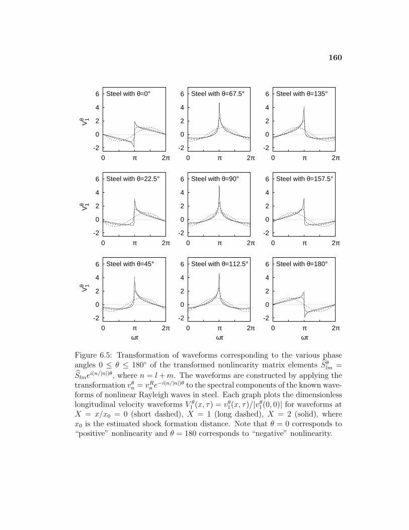
160
-2
0
2
4
6
0 π 2π
Steel with θ=0°
-2
0
2
4
6
0 π 2π
Steel with θ=22.5°
-2
0
2
4
6
0 π 2π
Steel with θ=45°
ωτ
-2
0
2
4
6
0 π 2π
Steel with θ=67.5°
-2
0
2
4
6
0 π 2π
Steel with θ=90°
-2
0
2
4
6
0 π 2π
Steel with θ=112.5°
ωτ
-2
0
2
4
6
0 π 2π
Steel with θ=135°
-2
0
2
4
6
0 π 2π
Steel with θ=157.5°
-2
0
2
4
6
0 π 2π
Steel with θ=180°
ωτ
V1θ
V1θ
V1θ
Figure 6.5: Transformation of waveforms corresponding to the various phaseangles 0 ≤ θ ≤ 180◦ of the transformed nonlinearity matrix elements Sθ
lm =
Slmei(n/|n|)θ, where n = l + m. The waveforms are constructed by applying thetransformation vθ
n = vRn e−i(n/|n|)θ to the spectral components of the known wave-
forms of nonlinear Rayleigh waves in steel. Each graph plots the dimensionlesslongitudinal velocity waveforms V θ
1 (x, τ) = vθ1(x, τ)/|vθ
1(0, 0)| for waveforms atX = x/x0 = 0 (short dashed), X = 1 (long dashed), X = 2 (solid), wherex0 is the estimated shock formation distance. Note that θ = 0 corresponds to“positive” nonlinearity and θ = 180 corresponds to “negative” nonlinearity.
161
-6
-4
-2
0
2
0 π 2π
Steel with θ=0°
-6
-4
-2
0
2
0 π 2π
Steel with θ=-22.5°
-6
-4
-2
0
2
0 π 2π
Steel with θ=-45°
ωτ
-6
-4
-2
0
2
0 π 2π
Steel with θ=-67.5°
-6
-4
-2
0
2
0 π 2π
Steel with θ=-90°
-6
-4
-2
0
2
0 π 2π
Steel with θ=-112.5°
ωτ
-6
-4
-2
0
2
0 π 2π
Steel with θ=-135°
-6
-4
-2
0
2
0 π 2π
Steel with θ=-157.5°
-6
-4
-2
0
2
0 π 2π
Steel with θ=-180°
ωτ
V1θ
V1θ
V1θ
Figure 6.6: Transformation of waveforms corresponding to the various phaseangles −180◦ ≥ θ ≥ 0 of the transformed nonlinearity matrix elementsSθ
lm = Slmei(n/|n|)θ. The waveforms are constructed by applying the transfor-mation vθ
n = vRn e−i(n/|n|)θ to the spectral components of the known waveforms
of nonlinear Rayleigh waves in steel. Each graph plots the dimensionless longi-tudinal velocity V θ
1 (x, τ) = vθ1(x, τ)/|vθ
1(0, 0)| for waveforms at X = x/x0 = 0(short dashed), X = 1 (long dashed), X = 2 (solid), where x0 is the esti-mated shock formation distance. Note that θ = 0 corresponds to “positive”nonlinearity and θ = −180 corresponds to “negative” nonlinearity.
162
When θ = −π/2, then Eq. (6.17) reduces to
vθ=−π/21 (x, τ) = H[vR
1 (x, τ)] , (6.18)
as required. The remaining plots show the expected waveform shapes for inter-
mediate values of θ and, therefore, other cases of complex-valued nonlinearity
matrix elements. (See Appendix F for additional discussion about complex-
valued nonlinearity parameters.)
As demonstrated above for the Rayleigh wave case, the tables are not
limited to longitudinal velocity waveforms. If the phase differences between
B1, B2, and B3 are known, then the corresponding waveform distortion in
the vertical and transverse directions can also be read from Figures 6.5. Let
θlong = arg(Slm) be the phase of the matrix elements (in the case that the
phase are not all the same, choose a representative element, typically S11). As
shown in Appendix F, the appropriate values of θtran and θvert to characterize
the transverse and vertical velocity waveforms are given by
θtran = arg(B1)− arg(B2) + θlong , (6.19a)
θvert = arg(B1)− arg(B3) + θlong . (6.19b)
In other words, these are the phases that are appropriate to use with Eq. (6.10)
and Figures 6.5 and 6.6 to determine the nature of the waveform distortion.
The true test of the interpretation is to apply it to real crystals. Fig-
ure 6.7 shows comparisons of the longitudinal waveforms in several real crystals
and the appropriately transformed and scaled waveforms of nonlinear Rayleigh
waves in steel. The figures of the transformed Rayleigh waves were constructed
via Eq. (6.10) in three steps:
1. The linear amplitude factor B1 and nonlinearity matrix element S11 were
computed for each crystal.
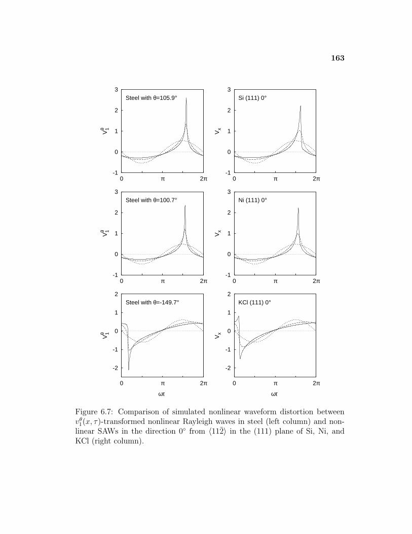
163
-1
0
1
2
3
0 π 2π
V1θ
Steel with θ=105.9°
-1
0
1
2
3
0 π 2π
V1θ
Steel with θ=100.7°
-2
-1
0
1
2
0 π 2π
V1θ
Steel with θ=-149.7°
ωτ
-1
0
1
2
3
0 π 2π
Vx
Si (111) 0°
-1
0
1
2
3
0 π 2π
Vx
Ni (111) 0°
-2
-1
0
1
2
0 π 2π
Vx
KCl (111) 0°
ωτ
Figure 6.7: Comparison of simulated nonlinear waveform distortion betweenvθ1(x, τ)-transformed nonlinear Rayleigh waves in steel (left column) and non-
linear SAWs in the direction 0◦ from 〈112〉 in the (111) plane of Si, Ni, andKCl (right column).
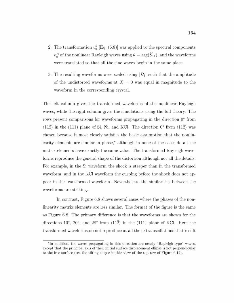
164
2. The transformation vθn [Eq. (6.8)] was applied to the spectral components
vRn of the nonlinear Rayleigh waves using θ = arg(S11), and the waveforms
were translated so that all the sine waves begin in the same place.
3. The resulting waveforms were scaled using |B1| such that the amplitude
of the undistorted waveforms at X = 0 was equal in magnitude to the
waveform in the corresponding crystal.
The left column gives the transformed waveforms of the nonlinear Rayleigh
waves, while the right column gives the simulations using the full theory. The
rows present comparisons for waveforms propagating in the direction 0◦ from
〈112〉 in the (111) plane of Si, Ni, and KCl. The direction 0◦ from 〈112〉 was
chosen because it most closely satisfies the basic assumption that the nonlin-
earity elements are similar in phase,∗ although in none of the cases do all the
matrix elements have exactly the same value. The transformed Rayleigh wave-
forms reproduce the general shape of the distortion although not all the details.
For example, in the Si waveform the shock is steeper than in the transformed
waveform, and in the KCl waveform the cusping before the shock does not ap-
pear in the transformed waveform. Nevertheless, the similarities between the
waveforms are striking.
In contrast, Figure 6.8 shows several cases where the phases of the non-
linearity matrix elements are less similar. The format of the figure is the same
as Figure 6.8. The primary difference is that the waveforms are shown for the
directions 10◦, 20◦, and 28◦ from 〈112〉 in the (111) plane of KCl. Here the
transformed waveforms do not reproduce at all the extra oscillations that result
∗In addition, the waves propagating in this direction are nearly “Rayleigh-type” waves,except that the principal axis of their initial surface displacement ellipse is not perpendicularto the free surface (see the tilting ellipse in side view of the top row of Figure 6.12).
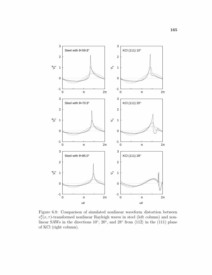
165
-1
0
1
2
3
0 π 2π
V1θ
Steel with θ=59.8°
-1
0
1
2
3
0 π 2π
V1θ
Steel with θ=70.9°
-1
0
1
2
3
0 π 2π
V1θ
Steel with θ=85.0°
ωτ
-1
0
1
2
3
0 π 2π
Vx
KCl (111) 10°
-1
0
1
2
3
0 π 2π
Vx
KCl (111) 20°
-1
0
1
2
3
0 π 2π
Vx
KCl (111) 28°
ωτ
Figure 6.8: Comparison of simulated nonlinear waveform distortion betweenvθ1(x, τ)-transformed nonlinear Rayleigh waves in steel (left column) and non-
linear SAWs in the directions 10◦, 20◦, and 28◦ from 〈112〉 in the (111) planeof KCl (right column).
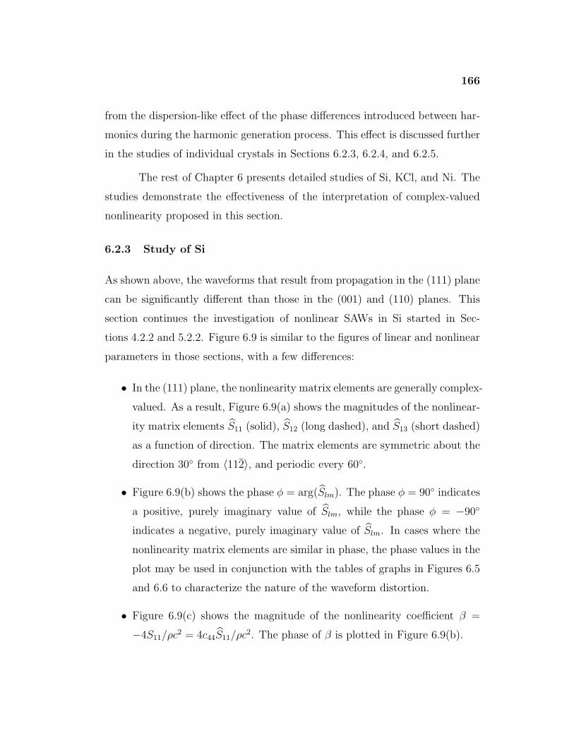
166
from the dispersion-like effect of the phase differences introduced between har-
monics during the harmonic generation process. This effect is discussed further
in the studies of individual crystals in Sections 6.2.3, 6.2.4, and 6.2.5.
The rest of Chapter 6 presents detailed studies of Si, KCl, and Ni. The
studies demonstrate the effectiveness of the interpretation of complex-valued
nonlinearity proposed in this section.
6.2.3 Study of Si
As shown above, the waveforms that result from propagation in the (111) plane
can be significantly different than those in the (001) and (110) planes. This
section continues the investigation of nonlinear SAWs in Si started in Sec-
tions 4.2.2 and 5.2.2. Figure 6.9 is similar to the figures of linear and nonlinear
parameters in those sections, with a few differences:
• In the (111) plane, the nonlinearity matrix elements are generally complex-
valued. As a result, Figure 6.9(a) shows the magnitudes of the nonlinear-
ity matrix elements S11 (solid), S12 (long dashed), and S13 (short dashed)
as a function of direction. The matrix elements are symmetric about the
direction 30◦ from 〈112〉, and periodic every 60◦.
• Figure 6.9(b) shows the phase φ = arg(Slm). The phase φ = 90◦ indicates
a positive, purely imaginary value of Slm, while the phase φ = −90◦
indicates a negative, purely imaginary value of Slm. In cases where the
nonlinearity matrix elements are similar in phase, the phase values in the
plot may be used in conjunction with the tables of graphs in Figures 6.5
and 6.6 to characterize the nature of the waveform distortion.
• Figure 6.9(c) shows the magnitude of the nonlinearity coefficient β =
−4S11/ρc2 = 4c44S11/ρc2. The phase of β is plotted in Figure 6.9(b).
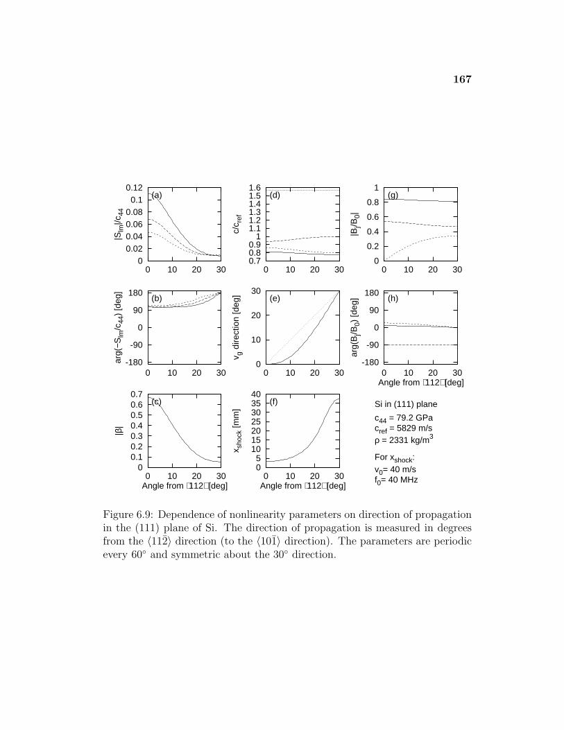
167
0 0.02 0.04 0.06 0.08 0.1
0.12
0 10 20 30
|Slm
|/c44
(a)
-180
-90
0
90
180
0 10 20 30
arg(
−Slm
/c44
) [d
eg]
(b)
0 0.1 0.2 0.3 0.4 0.5 0.6 0.7
0 10 20 30
|β|
(c)
Angle from ⟨112⟩ [deg]
0.7 0.8 0.9 1 1.1 1.2 1.3 1.4 1.5 1.6
0 10 20 30
c/c r
ef
(d)
0
10
20
30
0 10 20 30
v g d
irect
ion
[deg
] (e)
0 5 10 15 20 25 30 35 40
0 10 20 30
x sho
ck [m
m]
(f)
Angle from ⟨112⟩ [deg]
0
0.2
0.4
0.6
0.8
1
0 10 20 30
|Bj/B
0|
(g)
-180
-90
0
90
180
0 10 20 30
arg(
Bj/B
0) [d
eg] (h)
Angle from ⟨112⟩ [deg]
Si in (111) plane
c44 = 79.2 GPacref = 5829 m/sρ = 2331 kg/m3
For xshock:v0= 40 m/sf0= 40 MHz
Figure 6.9: Dependence of nonlinearity parameters on direction of propagationin the (111) plane of Si. The direction of propagation is measured in degreesfrom the 〈112〉 direction (to the 〈101〉 direction). The parameters are periodicevery 60◦ and symmetric about the 30◦ direction.
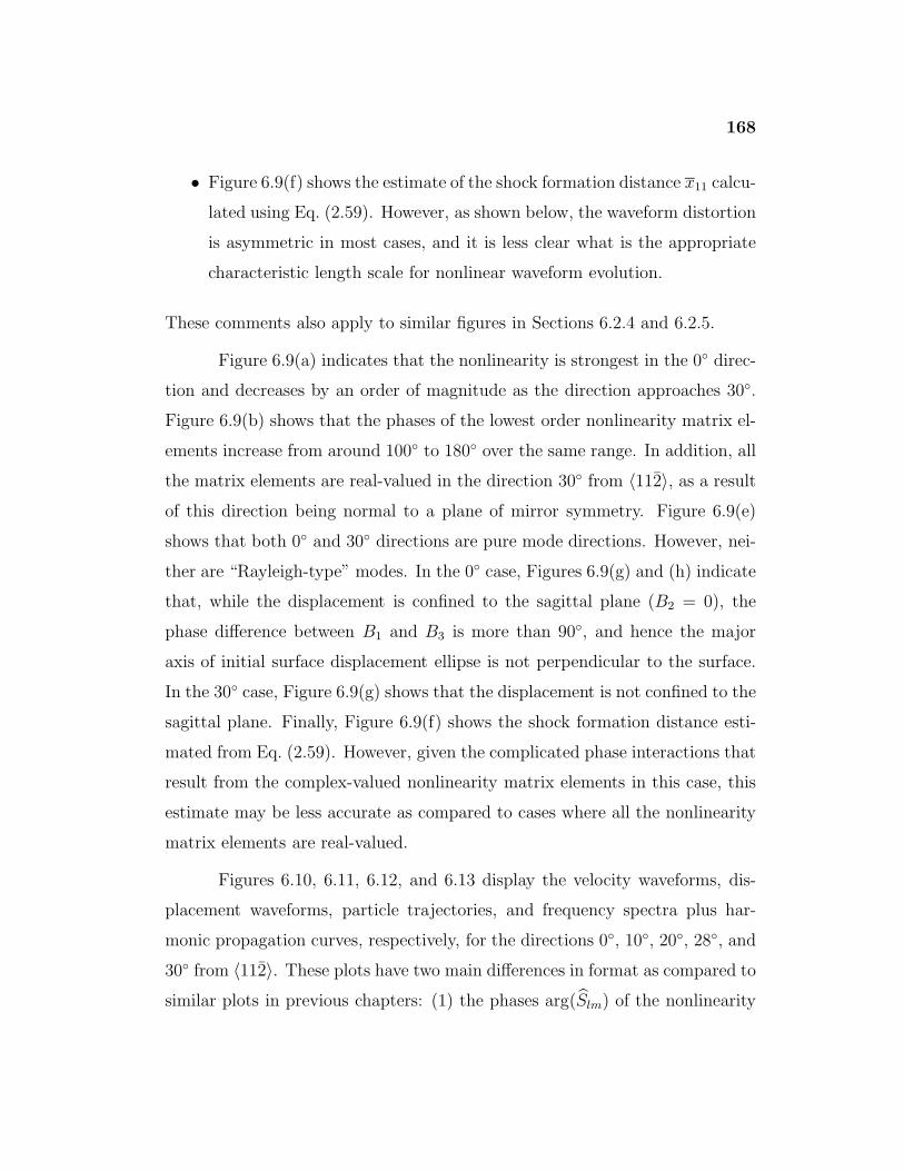
168
• Figure 6.9(f) shows the estimate of the shock formation distance x11 calcu-
lated using Eq. (2.59). However, as shown below, the waveform distortion
is asymmetric in most cases, and it is less clear what is the appropriate
characteristic length scale for nonlinear waveform evolution.
These comments also apply to similar figures in Sections 6.2.4 and 6.2.5.
Figure 6.9(a) indicates that the nonlinearity is strongest in the 0◦ direc-
tion and decreases by an order of magnitude as the direction approaches 30◦.
Figure 6.9(b) shows that the phases of the lowest order nonlinearity matrix el-
ements increase from around 100◦ to 180◦ over the same range. In addition, all
the matrix elements are real-valued in the direction 30◦ from 〈112〉, as a result
of this direction being normal to a plane of mirror symmetry. Figure 6.9(e)
shows that both 0◦ and 30◦ directions are pure mode directions. However, nei-
ther are “Rayleigh-type” modes. In the 0◦ case, Figures 6.9(g) and (h) indicate
that, while the displacement is confined to the sagittal plane (B2 = 0), the
phase difference between B1 and B3 is more than 90◦, and hence the major
axis of initial surface displacement ellipse is not perpendicular to the surface.
In the 30◦ case, Figure 6.9(g) shows that the displacement is not confined to the
sagittal plane. Finally, Figure 6.9(f) shows the shock formation distance esti-
mated from Eq. (2.59). However, given the complicated phase interactions that
result from the complex-valued nonlinearity matrix elements in this case, this
estimate may be less accurate as compared to cases where all the nonlinearity
matrix elements are real-valued.
Figures 6.10, 6.11, 6.12, and 6.13 display the velocity waveforms, dis-
placement waveforms, particle trajectories, and frequency spectra plus har-
monic propagation curves, respectively, for the directions 0◦, 10◦, 20◦, 28◦, and
30◦ from 〈112〉. These plots have two main differences in format as compared to
similar plots in previous chapters: (1) the phases arg(Slm) of the nonlinearity
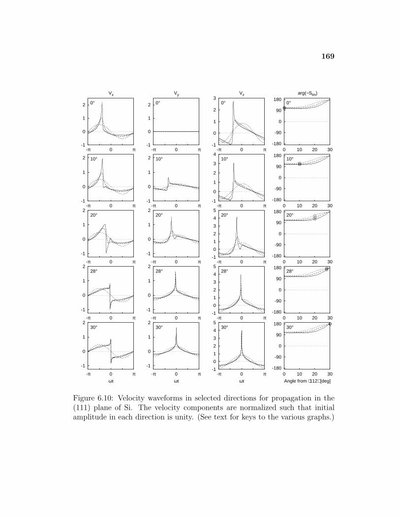
169
-1
0
1
2
-π 0 π
0°
Vx
-1
0
1
2
-π 0 π
0°
Vy
-1
0
1
2
3
-π 0 π
0°
Vz
-180
-90
0
90
180
0 10 20 30
arg(−Slm)
0°
-1
0
1
2
-π 0 π
10°
-1
0
1
2
-π 0 π
10°
-1
0
1
2
3
4
-π 0 π
10°
-180
-90
0
90
180
0 10 20 30
10°
-1
0
1
2
-π 0 π
20°
-1
0
1
2
-π 0 π
20°
-1
0
1
2
3
4
5
-π 0 π
20°
-180
-90
0
90
180
0 10 20 30
20°
-1
0
1
2
-π 0 π
28°
-1
0
1
2
-π 0 π
28°
-1
0
1
2
3
4
5
-π 0 π
28°
-180
-90
0
90
180
0 10 20 30
28°
-1
0
1
2
-π 0 π
30°
ωτ
-1
0
1
2
-π 0 π
30°
ωτ
-1
0
1
2
3
4
5
-π 0 π
30°
ωτ
-180
-90
0
90
180
0 10 20 30
30°
Angle from ⟨112⟩ [deg]
Nor
mal
ized
Vel
ocity
Wav
efor
ms
in (
111)
Pla
ne fo
r S
i
Figure 6.10: Velocity waveforms in selected directions for propagation in the(111) plane of Si. The velocity components are normalized such that initialamplitude in each direction is unity. (See text for keys to the various graphs.)
170
-0.6
-0.4
-0.2
0
0.2
-π 0 π
0°
Ux
-0.4
-0.2
0
0.2
0.4
-π 0 π
0°
Uy
-0.6
-0.4
-0.2
0
0.2
0.4
-π 0 π
0°
Uz
-180
-90
0
90
180
0 10 20 30
arg(−Slm)
0°
-0.6
-0.4
-0.2
0
0.2
-π 0 π
10°
-0.4
-0.2
0
0.2
0.4
-π 0 π
10°
-0.6
-0.4
-0.2
0
0.2
0.4
-π 0 π
10°
-180
-90
0
90
180
0 10 20 30
10°
-0.6
-0.4
-0.2
0
0.2
-π 0 π
20°
-0.4
-0.2
0
0.2
0.4
-π 0 π
20°
-0.6
-0.4
-0.2
0
0.2
0.4
-π 0 π
20°
-180
-90
0
90
180
0 10 20 30
20°
-0.6
-0.4
-0.2
0
0.2
-π 0 π
28°
-0.4
-0.2
0
0.2
0.4
-π 0 π
28°
-0.6
-0.4
-0.2
0
0.2
0.4
-π 0 π
28°
-180
-90
0
90
180
0 10 20 30
28°
-0.6
-0.4
-0.2
0
0.2
-π 0 π
30°
ωτ
-0.4
-0.2
0
0.2
0.4
-π 0 π
30°
ωτ
-0.6
-0.4
-0.2
0
0.2
0.4
-π 0 π
30°
ωτ
-180
-90
0
90
180
0 10 20 30
30°
Angle from ⟨112⟩ [deg]
Nor
mal
ized
Dis
plac
emen
t Wav
efor
ms
in (
111)
Pla
ne fo
r S
i
Figure 6.11: Displacement waveforms in selected directions of propagation inthe (111) plane of Si. The displacement components are computed by integrat-ing the velocity waveforms of Figure 6.10 over one cycle. (See text for keys tothe various graphs.)
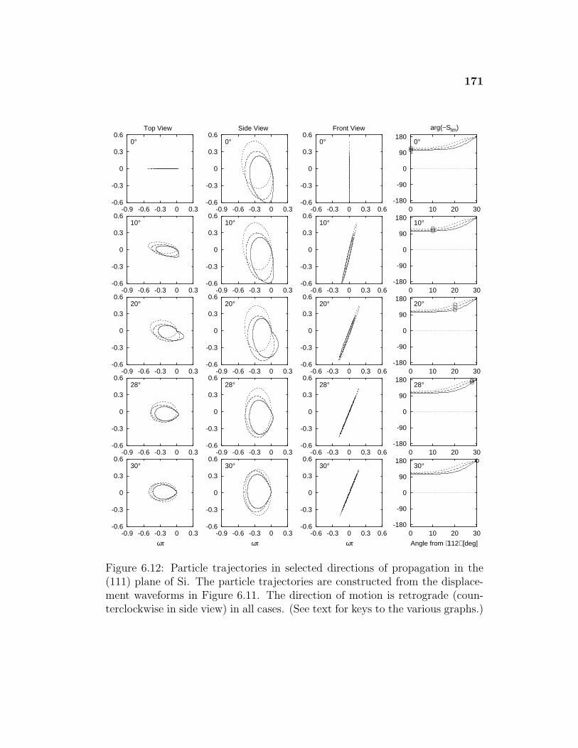
171
-0.6
-0.3
0
0.3
0.6
-0.9 -0.6 -0.3 0 0.3
0°
Top View
-0.6
-0.3
0
0.3
0.6
-0.9 -0.6 -0.3 0 0.3
0°
Side View
-0.6
-0.3
0
0.3
0.6
-0.6 -0.3 0 0.3 0.6
0°
Front View
-180
-90
0
90
180
0 10 20 30
arg(−Slm)
0°
-0.6
-0.3
0
0.3
0.6
-0.9 -0.6 -0.3 0 0.3
10°
-0.6
-0.3
0
0.3
0.6
-0.9 -0.6 -0.3 0 0.3
10°
-0.6
-0.3
0
0.3
0.6
-0.6 -0.3 0 0.3 0.6
10°
-180
-90
0
90
180
0 10 20 30
10°
-0.6
-0.3
0
0.3
0.6
-0.9 -0.6 -0.3 0 0.3
20°
-0.6
-0.3
0
0.3
0.6
-0.9 -0.6 -0.3 0 0.3
20°
-0.6
-0.3
0
0.3
0.6
-0.6 -0.3 0 0.3 0.6
20°
-180
-90
0
90
180
0 10 20 30
20°
-0.6
-0.3
0
0.3
0.6
-0.9 -0.6 -0.3 0 0.3
28°
-0.6
-0.3
0
0.3
0.6
-0.9 -0.6 -0.3 0 0.3
28°
-0.6
-0.3
0
0.3
0.6
-0.6 -0.3 0 0.3 0.6
28°
-180
-90
0
90
180
0 10 20 30
28°
-0.6
-0.3
0
0.3
0.6
-0.9 -0.6 -0.3 0 0.3
30°
ωτ
-0.6
-0.3
0
0.3
0.6
-0.9 -0.6 -0.3 0 0.3
30°
ωτ
-0.6
-0.3
0
0.3
0.6
-0.6 -0.3 0 0.3 0.6
30°
ωτ
-180
-90
0
90
180
0 10 20 30
30°
Angle from ⟨112⟩ [deg]
Nor
mal
ized
Par
ticle
Tra
ject
orie
s in
(11
1) P
lane
for
Si
Figure 6.12: Particle trajectories in selected directions of propagation in the(111) plane of Si. The particle trajectories are constructed from the displace-ment waveforms in Figure 6.11. The direction of motion is retrograde (coun-terclockwise in side view) in all cases. (See text for keys to the various graphs.)
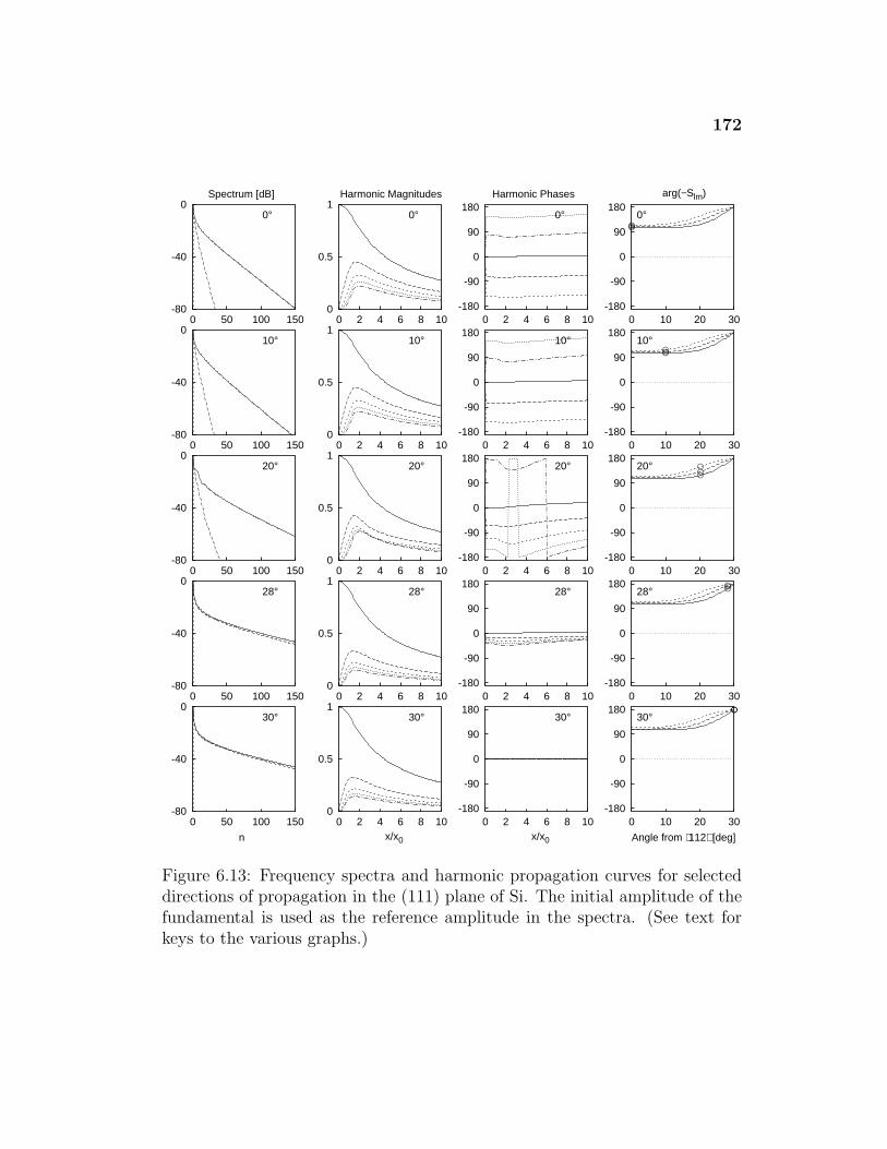
172
-80
-40
0
0 50 100 150
0°
Spectrum [dB]
0
0.5
1
0 2 4 6 8 10
0°
Harmonic Magnitudes
-180
-90
0
90
180
0 2 4 6 8 10
0°
Harmonic Phases
-180
-90
0
90
180
0 10 20 30
arg(−Slm)
0°
-80
-40
0
0 50 100 150
10°
0
0.5
1
0 2 4 6 8 10
10°
-180
-90
0
90
180
0 2 4 6 8 10
10°
-180
-90
0
90
180
0 10 20 30
10°
-80
-40
0
0 50 100 150
20°
0
0.5
1
0 2 4 6 8 10
20°
-180
-90
0
90
180
0 2 4 6 8 10
20°
-180
-90
0
90
180
0 10 20 30
20°
-80
-40
0
0 50 100 150
28°
0
0.5
1
0 2 4 6 8 10
28°
-180
-90
0
90
180
0 2 4 6 8 10
28°
-180
-90
0
90
180
0 10 20 30
28°
-80
-40
0
0 50 100 150
30°
n
0
0.5
1
0 2 4 6 8 10
30°
x/x0
-180
-90
0
90
180
0 2 4 6 8 10
30°
x/x0
-180
-90
0
90
180
0 10 20 30
30°
Angle from ⟨112⟩ [deg]
Spe
ctra
and
Har
mon
ic P
ropa
gatio
n C
urve
s in
(11
1) P
lane
for
Si
Figure 6.13: Frequency spectra and harmonic propagation curves for selecteddirections of propagation in the (111) plane of Si. The initial amplitude of thefundamental is used as the reference amplitude in the spectra. (See text forkeys to the various graphs.)
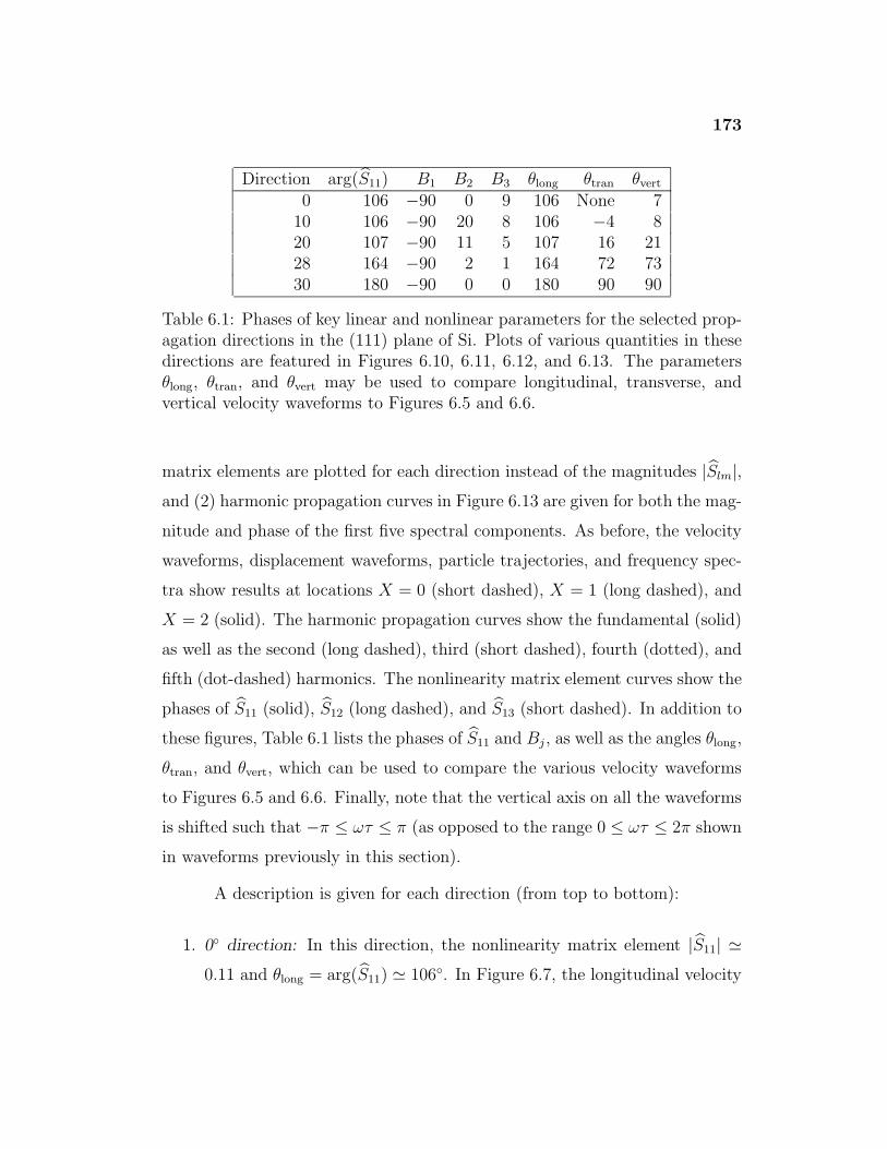
173
Direction arg(S11) B1 B2 B3 θlong θtran θvert
0 106 −90 0 9 106 None 710 106 −90 20 8 106 −4 820 107 −90 11 5 107 16 2128 164 −90 2 1 164 72 7330 180 −90 0 0 180 90 90
Table 6.1: Phases of key linear and nonlinear parameters for the selected prop-agation directions in the (111) plane of Si. Plots of various quantities in thesedirections are featured in Figures 6.10, 6.11, 6.12, and 6.13. The parametersθlong, θtran, and θvert may be used to compare longitudinal, transverse, andvertical velocity waveforms to Figures 6.5 and 6.6.
matrix elements are plotted for each direction instead of the magnitudes |Slm|,and (2) harmonic propagation curves in Figure 6.13 are given for both the mag-
nitude and phase of the first five spectral components. As before, the velocity
waveforms, displacement waveforms, particle trajectories, and frequency spec-
tra show results at locations X = 0 (short dashed), X = 1 (long dashed), and
X = 2 (solid). The harmonic propagation curves show the fundamental (solid)
as well as the second (long dashed), third (short dashed), fourth (dotted), and
fifth (dot-dashed) harmonics. The nonlinearity matrix element curves show the
phases of S11 (solid), S12 (long dashed), and S13 (short dashed). In addition to
these figures, Table 6.1 lists the phases of S11 and Bj , as well as the angles θlong,
θtran, and θvert, which can be used to compare the various velocity waveforms
to Figures 6.5 and 6.6. Finally, note that the vertical axis on all the waveforms
is shifted such that −π ≤ ωτ ≤ π (as opposed to the range 0 ≤ ωτ ≤ 2π shown
in waveforms previously in this section).
A description is given for each direction (from top to bottom):
1. 0◦ direction: In this direction, the nonlinearity matrix element |S11| '0.11 and θlong = arg(S11) ' 106◦. In Figure 6.7, the longitudinal velocity
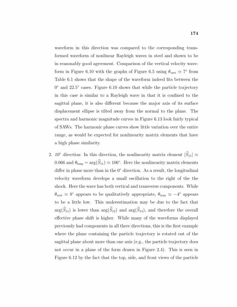
174
waveform in this direction was compared to the corresponding trans-
formed waveform of nonlinear Rayleigh waves in steel and shown to be
in reasonably good agreement. Comparison of the vertical velocity wave-
form in Figure 6.10 with the graphs of Figure 6.5 using θvert ' 7◦ from
Table 6.1 shows that the shape of the waveform indeed fits between the
0◦ and 22.5◦ cases. Figure 6.10 shows that while the particle trajectory
in this case is similar to a Rayleigh wave in that it is confined to the
sagittal plane, it is also different because the major axis of its surface
displacement ellipse is tilted away from the normal to the plane. The
spectra and harmonic magnitude curves in Figure 6.13 look fairly typical
of SAWs. The harmonic phase curves show little variation over the entire
range, as would be expected for nonlinearity matrix elements that have
a high phase similarity.
2. 10◦ direction: In this direction, the nonlinearity matrix element |S11| '0.066 and θlong = arg(S11) ' 106◦. Here the nonlinearity matrix elements
differ in phase more than in the 0◦ direction. As a result, the longitudinal
velocity waveform develops a small oscillation to the right of the the
shock. Here the wave has both vertical and transverse components. While
θvert ' 8◦ appears to be qualitatively appropriate, θtran ' −4◦ appears
to be a little low. This underestimation may be due to the fact that
arg(S11) is lower than arg(S12) and arg(S13), and therefore the overall
effective phase shift is higher. While many of the waveforms displayed
previously had components in all three directions, this is the first example
where the plane containing the particle trajectory is rotated out of the
sagittal plane about more than one axis (e.g., the particle trajectory does
not occur in a plane of the form drawn in Figure 2.4). This is seen in
Figure 6.12 by the fact that the top, side, and front views of the particle
175
trajectory are all elliptical. Figure 6.13 shows that the harmonic phase
curves develop a larger variation as compared to the previous direction.
3. 20◦ direction: In this direction, the nonlinearity matrix element |S11| '0.020 and θlong = arg(S11) ' 117◦. Here the phases of the nonlinearity
matrix elements have further separated. Figure 6.10 shows that this re-
sults in even larger oscillations to the right of the shocks and peaks in all
the velocity waveform components. As Figure 6.8 suggests, these wave-
forms are not reproduced well in detail by the simple vθn transformation
method described above and hence the values of θlong, θtran, and θvert are
less useful. Interestingly, Figure 6.12 shows that the oscillations cause
the particle trajectory to lose its elliptical form and develop into a shape
with a discontinuous tangent vector. Figure 6.13 indicates that spectra
develop small peaks in the lowest harmonics. The harmonic magnitude
curves for the third, fourth, and fifth harmonics move closer together than
in the previous directions, and the harmonic magnitude curves show more
variation and less regular spacing. Note that sharp vertical lines in the
fourth and fifth harmonics are actually discontinuities introduced by the
fact that −180◦ and +180◦ represent the same phase.
4. 28◦ direction: In this direction, the nonlinearity matrix element |S11| '0.0085 and θlong = arg(S11) ' 164◦. In this direction, the velocity wave-
forms begin to look more like the class of waveforms typified by the di-
rection 10◦ from 〈100〉 in the (001) plane of KCl. This occurs for several
reasons. First and foremost, the magnitude |S11| falls below |S12| and
|S13|, just like the previously mentioned case. Second, the phase of the
matrix elements have moved closer together compared to the case at 20◦,
as seen in Figure 6.13. This phase similarity causes the transformed
waveforms corresponding to the phases θtran and θvert to better match
176
the velocity waveforms in Figure 6.10, although they still appear a bit
underestimated. As expected, the frequency spectra indicate that energy
is transferred to the higher harmonics faster than is typical.
5. 30◦ direction: In this direction, the nonlinearity matrix element |S11| '0.0086 and θlong = arg(S11) = 180◦. Due to the symmetries of this direc-
tion, the nonlinearity matrix elements Slm are real-valued and negative
(phase of 180◦). The waveform distortion is “negative” but of the variety
described for the 28◦ direction. Note that the values of θlong, θtran, and
θvert given in Table 6.1 match the waveforms well, as would be expected
from the phase similarity of the nonlinearity matrix elements.
These simulations demonstrate that, in directions in which the phases of the
dominant nonlinearity matrix elements are similar, the velocity waveforms can
be characterized well by the transformations described in Section 6.2.2. Direc-
tions in which the nonlinearity matrix are less similar exhibit oscillations that
appear to right of the shocks and peaks in the velocity waveforms. Finally,
directions where the nonlinearity matrix elements are real-valued or nearly
real-valued exhibit distortion like that seen previously in the (001) and (110)
planes.
6.2.4 Study of KCl
Next, consider nonlinear SAWs in the (111) plane of KCl. Figure 6.14 displays
the linear and nonlinear parameters describing propagation in this plane. Fig-
ure 6.14(a) shows that the magnitudes of the nonlinearity matrix elements are
highest in the 0◦ direction, they dip down to a local minimum around 3◦, rise
to a local maximum around 10◦, and then fall off to a global minimum at 30◦
which is approximately an order of magnitude smaller than at 0◦. The direc-
tion where the local minimum occurs coincides with the direction where the
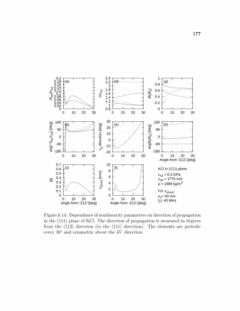
177
0 0.02 0.04 0.06 0.08 0.1
0.12 0.14 0.16 0.18 0.2
0 10 20 30
|Slm
|/c44
(a)
-180
-90
0
90
180
0 10 20 30
arg(
−Slm
/c44
) [d
eg]
(b)
0 0.1 0.2 0.3 0.4 0.5 0.6 0.7
0 10 20 30
|β|
(c)
Angle from ⟨112⟩ [deg]
0.8 1
1.2 1.4 1.6 1.8 2
2.2 2.4
0 10 20 30
c/c r
ef
(d)
-20
-10
0
10
20
30
0 10 20 30
v g d
irect
ion
[deg
] (e)
0
2
4
6
8
10
0 10 20 30
x sho
ck [m
m]
(f)
Angle from ⟨112⟩ [deg]
0
0.2
0.4
0.6
0.8
1
0 10 20 30
|Bj/B
0|
(g)
-180
-90
0
90
180
0 10 20 30
arg(
Bj/B
0) [d
eg] (h)
Angle from ⟨112⟩ [deg]
KCl in (111) plane
c44 = 6.3 GPacref = 1775 m/sρ = 1989 kg/m3
For xshock:v0= 40 m/sf0= 40 MHz
Figure 6.14: Dependence of nonlinearity parameters on direction of propagationin the (111) plane of KCl. The direction of propagation is measured in degreesfrom the 〈112〉 direction (to the 〈111〉 direction). The elements are periodicevery 30◦ and symmetric about the 45◦ direction.
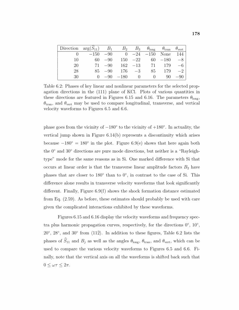
178
Direction arg(S11) B1 B2 B3 θlong θtran θvert
0 −150 −90 0 −24 −150 None 14410 60 −90 150 −22 60 −180 −820 71 −90 162 −13 71 179 −628 85 −90 176 −3 85 179 −230 0 −90 −180 0 0 90 −90
Table 6.2: Phases of key linear and nonlinear parameters for the selected prop-agation directions in the (111) plane of KCl. Plots of various quantities inthese directions are featured in Figures 6.15 and 6.16. The parameters θlong,θtran, and θvert may be used to compare longitudinal, transverse, and verticalvelocity waveforms to Figures 6.5 and 6.6.
phase goes from the vicinity of −180◦ to the vicinity of +180◦. In actuality, the
vertical jump shown in Figure 6.14(b) represents a discontinuity which arises
because −180◦ = 180◦ in the plot. Figure 6.9(e) shows that here again both
the 0◦ and 30◦ directions are pure mode directions, but neither is a “Rayleigh-
type” mode for the same reasons as in Si. One marked difference with Si that
occurs at linear order is that the transverse linear amplitude factors B2 have
phases that are closer to 180◦ than to 0◦, in contrast to the case of Si. This
difference alone results in transverse velocity waveforms that look significantly
different. Finally, Figure 6.9(f) shows the shock formation distance estimated
from Eq. (2.59). As before, these estimates should probably be used with care
given the complicated interactions exhibited by these waveforms.
Figures 6.15 and 6.16 display the velocity waveforms and frequency spec-
tra plus harmonic propagation curves, respectively, for the directions 0◦, 10◦,
20◦, 28◦, and 30◦ from 〈112〉. In addition to these figures, Table 6.2 lists the
phases of S11 and Bj as well as the angles θlong, θtran, and θvert, which can be
used to compare the various velocity waveforms to Figures 6.5 and 6.6. Fi-
nally, note that the vertical axis on all the waveforms is shifted back such that
0 ≤ ωτ ≤ 2π.
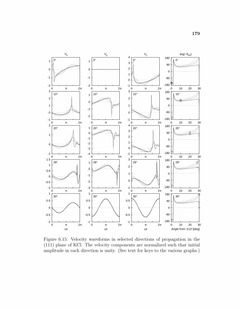
179
-2
-1
0
1
0 π 2π
0°
Vx
-2
-1
0
1
0 π 2π
0°
Vy
-1
0
1
2
3
4
0 π 2π
0°
Vz
-180
-90
0
90
180
0 10 20 30
arg(−Slm)
0°
-1
0
1
2
3
0 π 2π
10°
-2
-1
0
1
0 π 2π
10°
-1
0
1
2
3
0 π 2π
10°
-180
-90
0
90
180
0 10 20 30
10°
-1
0
1
2
0 π 2π
20°
-4
-3
-2
-1
0
1
0 π 2π
20°
-1
0
1
2
3
4
0 π 2π
20°
-180
-90
0
90
180
0 10 20 30
20°
-1
-0.5
0
0.5
1
1.5
0 π 2π
28°
-3
-2
-1
0
1
0 π 2π
28°
-1
0
1
2
3
0 π 2π
28°
-180
-90
0
90
180
0 10 20 30
28°
-1
-0.5
0
0.5
1
0 π 2π
30°
ωτ
-1
-0.5
0
0.5
1
0 π 2π
30°
ωτ
-1
-0.5
0
0.5
1
0 π 2π
30°
ωτ
-180
-90
0
90
180
0 10 20 30
30°
Angle from ⟨112⟩ [deg]
Nor
mal
ized
Vel
ocity
Wav
efor
ms
in (
111)
Pla
ne fo
r K
Cl
Figure 6.15: Velocity waveforms in selected directions of propagation in the(111) plane of KCl. The velocity components are normalized such that initialamplitude in each direction is unity. (See text for keys to the various graphs.)
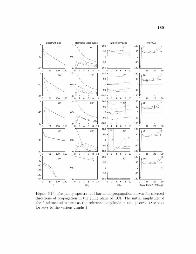
180
-80
-40
0
0 50 100 150
0°
Spectrum [dB]
0
0.5
1
0 2 4 6 8 10
0°
Harmonic Magnitudes
-180
-90
0
90
180
0 2 4 6 8 10
0°
Harmonic Phases
-180
-90
0
90
180
0 10 20 30
arg(−Slm)
0°
-80
-40
0
0 50 100 150
10°
0
0.5
1
0 2 4 6 8 10
10°
-180
-90
0
90
180
0 2 4 6 8 10
10°
-180
-90
0
90
180
0 10 20 30
10°
-80
-40
0
0 50 100 150
20°
0
0.5
1
0 2 4 6 8 10
20°
-180
-90
0
90
180
0 2 4 6 8 10
20°
-180
-90
0
90
180
0 10 20 30
20°
-80
-40
0
0 50 100 150
28°
0
0.5
1
0 2 4 6 8 10
28°
-180
-90
0
90
180
0 2 4 6 8 10
28°
-180
-90
0
90
180
0 10 20 30
28°
-200
-160
-120
-80
-40
0
0 50 100 150
30°
n
0
0.5
1
0 2 4 6 8 10
30°
x/x0
-180
-90
0
90
180
0 2 4 6 8 10
30°
x/x0
-180
-90
0
90
180
0 10 20 30
30°
Angle from ⟨112⟩ [deg]
Spe
ctra
and
Har
mon
ic P
ropa
gatio
n C
urve
s in
(11
1) P
lane
for
KC
l
Figure 6.16: Frequency spectra and harmonic propagation curves for selecteddirections of propagation in the (111) plane of KCl. The initial amplitude ofthe fundamental is used as the reference amplitude in the spectra. (See textfor keys to the various graphs.)
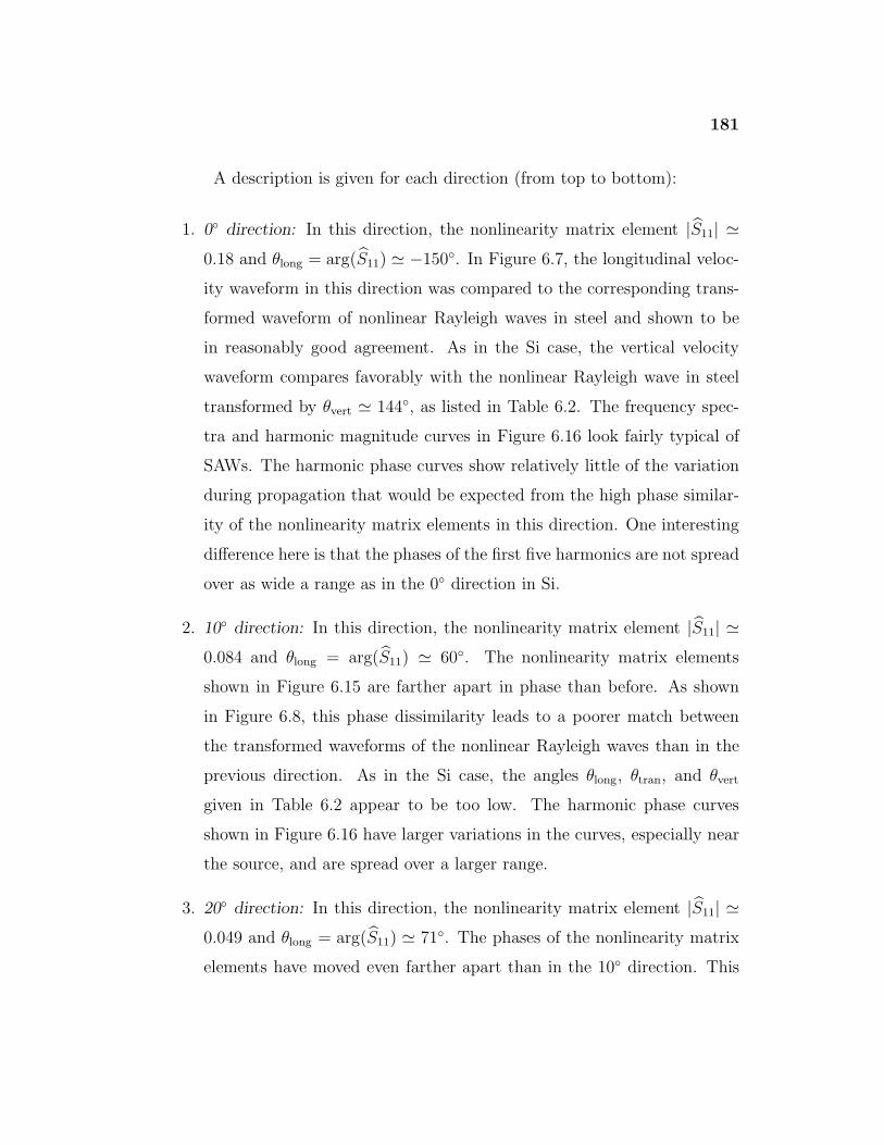
181
A description is given for each direction (from top to bottom):
1. 0◦ direction: In this direction, the nonlinearity matrix element |S11| '0.18 and θlong = arg(S11) ' −150◦. In Figure 6.7, the longitudinal veloc-
ity waveform in this direction was compared to the corresponding trans-
formed waveform of nonlinear Rayleigh waves in steel and shown to be
in reasonably good agreement. As in the Si case, the vertical velocity
waveform compares favorably with the nonlinear Rayleigh wave in steel
transformed by θvert ' 144◦, as listed in Table 6.2. The frequency spec-
tra and harmonic magnitude curves in Figure 6.16 look fairly typical of
SAWs. The harmonic phase curves show relatively little of the variation
during propagation that would be expected from the high phase similar-
ity of the nonlinearity matrix elements in this direction. One interesting
difference here is that the phases of the first five harmonics are not spread
over as wide a range as in the 0◦ direction in Si.
2. 10◦ direction: In this direction, the nonlinearity matrix element |S11| '0.084 and θlong = arg(S11) ' 60◦. The nonlinearity matrix elements
shown in Figure 6.15 are farther apart in phase than before. As shown
in Figure 6.8, this phase dissimilarity leads to a poorer match between
the transformed waveforms of the nonlinear Rayleigh waves than in the
previous direction. As in the Si case, the angles θlong, θtran, and θvert
given in Table 6.2 appear to be too low. The harmonic phase curves
shown in Figure 6.16 have larger variations in the curves, especially near
the source, and are spread over a larger range.
3. 20◦ direction: In this direction, the nonlinearity matrix element |S11| '0.049 and θlong = arg(S11) ' 71◦. The phases of the nonlinearity matrix
elements have moved even farther apart than in the 10◦ direction. This
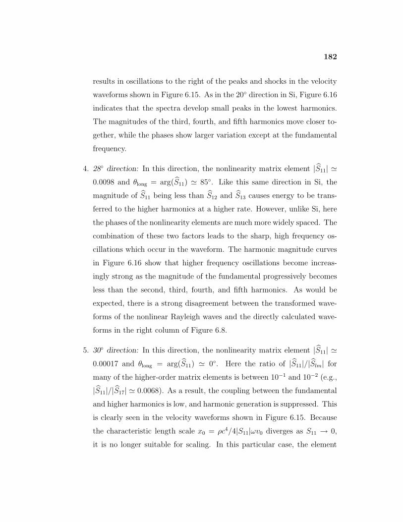
182
results in oscillations to the right of the peaks and shocks in the velocity
waveforms shown in Figure 6.15. As in the 20◦ direction in Si, Figure 6.16
indicates that the spectra develop small peaks in the lowest harmonics.
The magnitudes of the third, fourth, and fifth harmonics move closer to-
gether, while the phases show larger variation except at the fundamental
frequency.
4. 28◦ direction: In this direction, the nonlinearity matrix element |S11| '0.0098 and θlong = arg(S11) ' 85◦. Like this same direction in Si, the
magnitude of S11 being less than S12 and S13 causes energy to be trans-
ferred to the higher harmonics at a higher rate. However, unlike Si, here
the phases of the nonlinearity elements are much more widely spaced. The
combination of these two factors leads to the sharp, high frequency os-
cillations which occur in the waveform. The harmonic magnitude curves
in Figure 6.16 show that higher frequency oscillations become increas-
ingly strong as the magnitude of the fundamental progressively becomes
less than the second, third, fourth, and fifth harmonics. As would be
expected, there is a strong disagreement between the transformed wave-
forms of the nonlinear Rayleigh waves and the directly calculated wave-
forms in the right column of Figure 6.8.
5. 30◦ direction: In this direction, the nonlinearity matrix element |S11| '0.00017 and θlong = arg(S11) ' 0◦. Here the ratio of |S11|/|Slm| for
many of the higher-order matrix elements is between 10−1 and 10−2 (e.g.,
|S11|/|S17| ' 0.0068). As a result, the coupling between the fundamental
and higher harmonics is low, and harmonic generation is suppressed. This
is clearly seen in the velocity waveforms shown in Figure 6.15. Because
the characteristic length scale x0 = ρc4/4|S11|ωv0 diverges as S11 → 0,
it is no longer suitable for scaling. In this particular case, the element
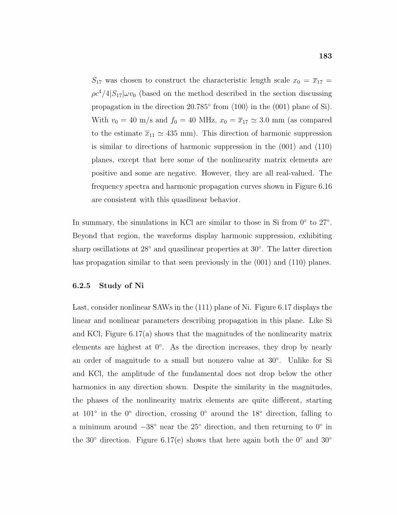
183
S17 was chosen to construct the characteristic length scale x0 = x17 =
ρc4/4|S17|ωv0 (based on the method described in the section discussing
propagation in the direction 20.785◦ from 〈100〉 in the (001) plane of Si).
With v0 = 40 m/s and f0 = 40 MHz, x0 = x17 ' 3.0 mm (as compared
to the estimate x11 ' 435 mm). This direction of harmonic suppression
is similar to directions of harmonic suppression in the (001) and (110)
planes, except that here some of the nonlinearity matrix elements are
positive and some are negative. However, they are all real-valued. The
frequency spectra and harmonic propagation curves shown in Figure 6.16
are consistent with this quasilinear behavior.
In summary, the simulations in KCl are similar to those in Si from 0◦ to 27◦.
Beyond that region, the waveforms display harmonic suppression, exhibiting
sharp oscillations at 28◦ and quasilinear properties at 30◦. The latter direction
has propagation similar to that seen previously in the (001) and (110) planes.
6.2.5 Study of Ni
Last, consider nonlinear SAWs in the (111) plane of Ni. Figure 6.17 displays the
linear and nonlinear parameters describing propagation in this plane. Like Si
and KCl, Figure 6.17(a) shows that the magnitudes of the nonlinearity matrix
elements are highest at 0◦. As the direction increases, they drop by nearly
an order of magnitude to a small but nonzero value at 30◦. Unlike for Si
and KCl, the amplitude of the fundamental does not drop below the other
harmonics in any direction shown. Despite the similarity in the magnitudes,
the phases of the nonlinearity matrix elements are quite different, starting
at 101◦ in the 0◦ direction, crossing 0◦ around the 18◦ direction, falling to
a minimum around −38◦ near the 25◦ direction, and then returning to 0◦ in
the 30◦ direction. Figure 6.17(e) shows that here again both the 0◦ and 30◦
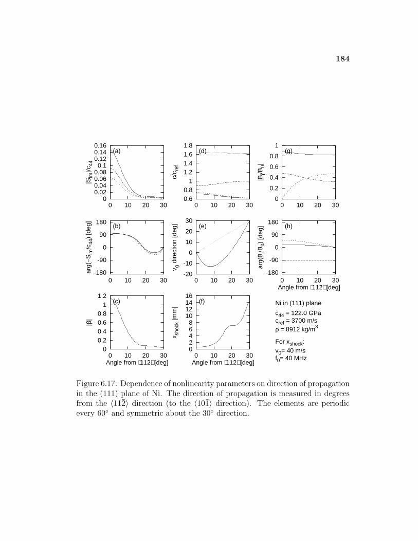
184
0 0.02 0.04 0.06 0.08 0.1
0.12 0.14 0.16
0 10 20 30
|Slm
|/c44
(a)
-180
-90
0
90
180
0 10 20 30
arg(
−Slm
/c44
) [d
eg]
(b)
0 0.2 0.4 0.6 0.8 1
1.2
0 10 20 30
|β|
(c)
Angle from ⟨112⟩ [deg]
0.6 0.8 1
1.2 1.4 1.6 1.8
0 10 20 30
c/c r
ef
(d)
-20
-10
0
10
20
30
0 10 20 30
v g d
irect
ion
[deg
] (e)
0 2 4 6 8
10 12 14 16
0 10 20 30
x sho
ck [m
m]
(f)
Angle from ⟨112⟩ [deg]
0
0.2
0.4
0.6
0.8
1
0 10 20 30
|Bj/B
0|
(g)
-180
-90
0
90
180
0 10 20 30
arg(
Bj/B
0) [d
eg] (h)
Angle from ⟨112⟩ [deg]
Ni in (111) plane
c44 = 122.0 GPacref = 3700 m/sρ = 8912 kg/m3
For xshock:v0= 40 m/sf0= 40 MHz
Figure 6.17: Dependence of nonlinearity parameters on direction of propagationin the (111) plane of Ni. The direction of propagation is measured in degreesfrom the 〈112〉 direction (to the 〈101〉 direction). The elements are periodicevery 60◦ and symmetric about the 30◦ direction.
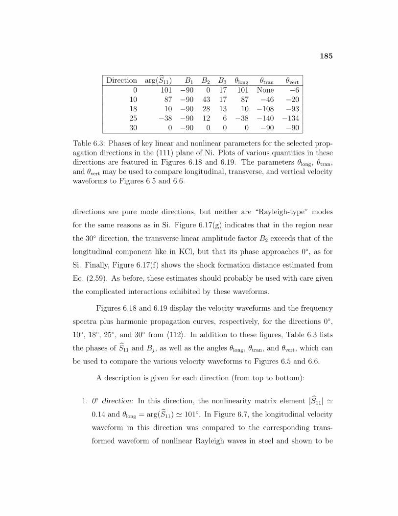
185
Direction arg(S11) B1 B2 B3 θlong θtran θvert
0 101 −90 0 17 101 None −610 87 −90 43 17 87 −46 −2018 10 −90 28 13 10 −108 −9325 −38 −90 12 6 −38 −140 −13430 0 −90 0 0 0 −90 −90
Table 6.3: Phases of key linear and nonlinear parameters for the selected prop-agation directions in the (111) plane of Ni. Plots of various quantities in thesedirections are featured in Figures 6.18 and 6.19. The parameters θlong, θtran,and θvert may be used to compare longitudinal, transverse, and vertical velocitywaveforms to Figures 6.5 and 6.6.
directions are pure mode directions, but neither are “Rayleigh-type” modes
for the same reasons as in Si. Figure 6.17(g) indicates that in the region near
the 30◦ direction, the transverse linear amplitude factor B2 exceeds that of the
longitudinal component like in KCl, but that its phase approaches 0◦, as for
Si. Finally, Figure 6.17(f) shows the shock formation distance estimated from
Eq. (2.59). As before, these estimates should probably be used with care given
the complicated interactions exhibited by these waveforms.
Figures 6.18 and 6.19 display the velocity waveforms and the frequency
spectra plus harmonic propagation curves, respectively, for the directions 0◦,
10◦, 18◦, 25◦, and 30◦ from 〈112〉. In addition to these figures, Table 6.3 lists
the phases of S11 and Bj , as well as the angles θlong, θtran, and θvert, which can
be used to compare the various velocity waveforms to Figures 6.5 and 6.6.
A description is given for each direction (from top to bottom):
1. 0◦ direction: In this direction, the nonlinearity matrix element |S11| '0.14 and θlong = arg(S11) ' 101◦. In Figure 6.7, the longitudinal velocity
waveform in this direction was compared to the corresponding trans-
formed waveform of nonlinear Rayleigh waves in steel and shown to be
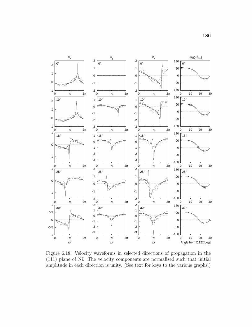
186
-1
0
1
2
0 π 2π
0°
Vx
-2
-1
0
1
2
0 π 2π
0°
Vy
-2
-1
0
1
2
0 π 2π
0°
Vz
-180
-90
0
90
180
0 10 20 30
arg(−Slm)
0°
-1
0
1
2
0 π 2π
10°
-3
-2
-1
0
1
0 π 2π
10°
-3
-2
-1
0
1
0 π 2π
10°
-180
-90
0
90
180
0 10 20 30
10°
-1
0
1
0 π 2π
18°
-3
-2
-1
0
1
0 π 2π
18°
-3
-2
-1
0
1
0 π 2π
18°
-180
-90
0
90
180
0 10 20 30
18°
-1
0
1
0 π 2π
25°
-2
-1
0
1
2
0 π 2π
25°
-2
-1
0
1
2
0 π 2π
25°
-180
-90
0
90
180
0 10 20 30
25°
-1
-0.5
0
0.5
1
0 π 2π
30°
ωτ
-3
-2
-1
0
1
2
0 π 2π
30°
ωτ
-3
-2
-1
0
1
2
0 π 2π
30°
ωτ
-180
-90
0
90
180
0 10 20 30
30°
Angle from ⟨112⟩ [deg]
Nor
mal
ized
Vel
ocity
Wav
efor
ms
in (
111)
Pla
ne fo
r N
i
Figure 6.18: Velocity waveforms in selected directions of propagation in the(111) plane of Ni. The velocity components are normalized such that initialamplitude in each direction is unity. (See text for keys to the various graphs.)
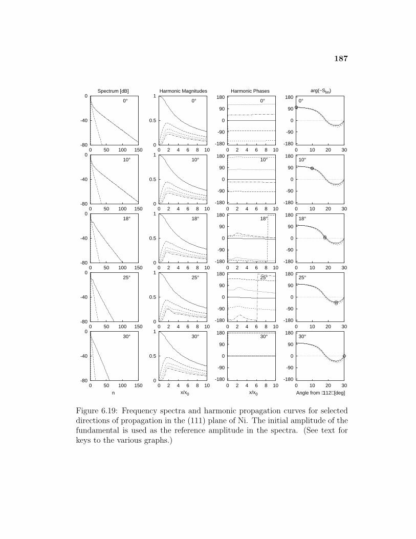
187
-80
-40
0
0 50 100 150
0°
Spectrum [dB]
0
0.5
1
0 2 4 6 8 10
0°
Harmonic Magnitudes
-180
-90
0
90
180
0 2 4 6 8 10
0°
Harmonic Phases
-180
-90
0
90
180
0 10 20 30
arg(−Slm)
0°
-80
-40
0
0 50 100 150
10°
0
0.5
1
0 2 4 6 8 10
10°
-180
-90
0
90
180
0 2 4 6 8 10
10°
-180
-90
0
90
180
0 10 20 30
10°
-80
-40
0
0 50 100 150
18°
0
0.5
1
0 2 4 6 8 10
18°
-180
-90
0
90
180
0 2 4 6 8 10
18°
-180
-90
0
90
180
0 10 20 30
18°
-80
-40
0
0 50 100 150
25°
0
0.5
1
0 2 4 6 8 10
25°
-180
-90
0
90
180
0 2 4 6 8 10
25°
-180
-90
0
90
180
0 10 20 30
25°
-80
-40
0
0 50 100 150
30°
n
0
0.5
1
0 2 4 6 8 10
30°
x/x0
-180
-90
0
90
180
0 2 4 6 8 10
30°
x/x0
-180
-90
0
90
180
0 10 20 30
30°
Angle from ⟨112⟩ [deg]
Spe
ctra
and
Har
mon
ic P
ropa
gatio
n C
urve
s in
(11
1) P
lane
for
Ni
Figure 6.19: Frequency spectra and harmonic propagation curves for selecteddirections of propagation in the (111) plane of Ni. The initial amplitude of thefundamental is used as the reference amplitude in the spectra. (See text forkeys to the various graphs.)
188
in reasonably good agreement. As in the Si case, the vertical velocity
waveform compares favorably with the nonlinear Rayleigh wave in steel
transformed by θvert ' −6◦, as listed in Table 6.3. The spectra and har-
monic magnitude curves in Figure 6.16 look fairly typical of SAWs. The
harmonic phase curves show relatively little variation during propagation
as would be expected from the high phase similarity of the nonlinearity
matrix elements in this direction.
2. 10◦ direction: In this direction, the nonlinearity matrix element |S11| '0.045 and θlong = arg(S11) ' 87◦. Unlike this direction in the other
crystals considered, the nonlinearity matrix elements are still quite similar
in phase in this direction. As a result, use of the angles θlong, θtran, and
θvert from Table 6.3 to compare the waveforms of Figure 6.18 with the
the transformed waveforms of Figures 6.5 and 6.6 yields favorable results.
Figure 6.19 shows that the harmonic phase curves show little variation
although, except for the fundamental, they are shifted upward slightly as
compared to the 0◦ direction.
3. 18◦ direction: In this direction, the nonlinearity matrix element |S11| '0.00783 and θlong = arg(S11) ' 10◦. Here the nonlinearity matrix ele-
ments start to separate more in phase. This dissimilarity gives rise to the
same result as before, namely, that the waveforms develop oscillations
near the shocks and peaks. One difference between this case and similar
cases in Si and KCl is that here the oscillations form to the left of the
shocks and peaks. This may be due to the fact that the phases of the
matrix elements S12 and S13 are less than S11 instead of more. Note that
the phases of all the nonlinearity matrix elements are near zero, which
indicates that the waveforms should look roughly like “positively” distort-
ing Rayleigh waves. If the oscillations are factored out of the waveforms
189
in Figure 6.18, this “positively” distorting trend can be seen (with some
imagination), especially in the vertical velocity component (θvert ' 93◦).
Figure 6.18 shows peaks in the frequency spectra and more variation in
the harmonic phase curves, especially near the source. The phases of
the odd harmonics are grouped around 0◦ and the even harmonics are
grouped around −180◦.
4. 25◦ direction: In this direction, the nonlinearity matrix element |S11| '0.0035 and θlong = arg(S11) ' −38◦. The nonlinearity matrix elements
are farther apart in phase here than in the 18◦ direction and, as shown
in Figure 6.18, this difference results in even larger oscillations near the
shocks and peaks. Figure 6.19 shows peaks in the frequency spectra and
larger variations in the harmonic phase curves. Note, however, that the
lower magnitudes of the nonlinearity matrix elements result in energy
being transferred to the higher harmonics at a decreased rate, as seen in
the frequency spectra in comparison to the 0◦ and 10◦ cases.
5. 30◦ direction: In this direction, the nonlinearity matrix element |S11| '0.0035 and θlong = arg(S11) ' 0◦. All the nonlinearity matrix elements
are real-valued in this direction. Most of the matrix elements Slm which
describe coupling between the lowest harmonics are positive, although
although some of the higher elements are negative. As seen in Figure 6.18,
this results in waveforms that distort in the “positive” manner seen in
the (001) and (110) planes. Note that the values of θlong, θtran, and θvert
given in Table 6.1 match the waveforms well, as would be expected from
the phase similarity of the nonlinearity matrix elements. Similar to the
25◦ direction, the frequency spectra in Figure 6.18 show that less energy
is transferred to the higher harmonics due to the reduced magnitudes of
the nonlinearity matrix elements. Examination of the harmonic phases
190
shows that the odd harmonics are positive and the even harmonics are
negative. This information is collapsed into the two lines at 0◦ and 180◦
in the harmonic phase curves.
In summary, the simulations in Ni show many features in common with Si
and KCl, including the appearance of oscillations in the velocity waveforms
where the nonlinearity matrix elements are less similar in phase, and distortion
that is similar to (001) and (110) planes near the 30◦ direction. The most
significant difference for Ni is that in the directions where oscillations form in
the waveforms, they form to the right of the peaks and shocks, instead of to
the left.
6.3 Summary
This chapter has studied the propagation of nonlinear SAWs in the (111) plane
for a variety of cubic crystals. The SAWs in this plane differ from those in the
(001) and (110) planes in that the nonlinearity matrix elements are generally
complex-valued. A simple mathematical transformation was shown to provide
an interpretation of the phase information contained in the nonlinearity ma-
trix elements and linear amplitude factors. Comparisons were made between
waveforms approximated by this method and those generated with the full sim-
ulation. The match was shown to be best when most of the nonlinearity matrix
elements of the crystals have the same or approximately the same phase. As
in previous chapters, it was demonstrated that plots of the nonlinearity matrix
elements as a function of direction can be used as an indication of the harmonic
generation and waveform distortion. In most directions, the waveforms distort
asymmetrically and, in some cases, the dissimilar phases of the nonlinearity
matrix elements cause a nonlinear dispersion-like effect whereby oscillations

191
form in the vicinity of the shocks and peaks of the velocity waveforms. De-
tailed analysis was provided for Si, KCl, and Ni, with other crystals expected
to exhibit similar effects.
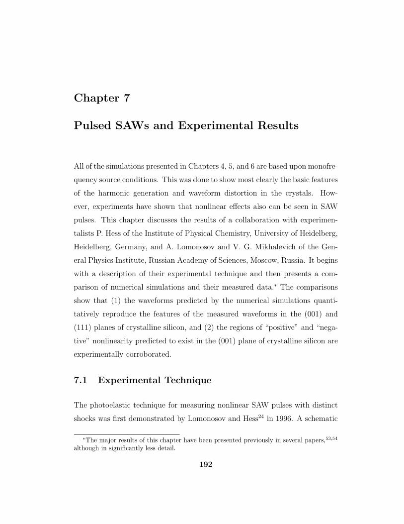
Chapter 7
Pulsed SAWs and Experimental Results
All of the simulations presented in Chapters 4, 5, and 6 are based upon monofre-
quency source conditions. This was done to show most clearly the basic features
of the harmonic generation and waveform distortion in the crystals. How-
ever, experiments have shown that nonlinear effects also can be seen in SAW
pulses. This chapter discusses the results of a collaboration with experimen-
talists P. Hess of the Institute of Physical Chemistry, University of Heidelberg,
Heidelberg, Germany, and A. Lomonosov and V. G. Mikhalevich of the Gen-
eral Physics Institute, Russian Academy of Sciences, Moscow, Russia. It begins
with a description of their experimental technique and then presents a com-
parison of numerical simulations and their measured data.∗ The comparisons
show that (1) the waveforms predicted by the numerical simulations quanti-
tatively reproduce the features of the measured waveforms in the (001) and
(111) planes of crystalline silicon, and (2) the regions of “positive” and “nega-
tive” nonlinearity predicted to exist in the (001) plane of crystalline silicon are
experimentally corroborated.
7.1 Experimental Technique
The photoelastic technique for measuring nonlinear SAW pulses with distinct
shocks was first demonstrated by Lomonosov and Hess24 in 1996. A schematic
∗The major results of this chapter have been presented previously in several papers,53,54
although in significantly less detail.
192
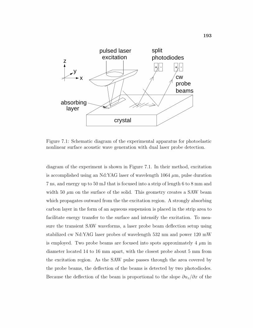
193
++ --
xy
z
crystal
splitphotodiodes
beamsprobe
absorbinglayer
cw
excitationpulsed laser
Figure 7.1: Schematic diagram of the experimental apparatus for photoelasticnonlinear surface acoustic wave generation with dual laser probe detection.
diagram of the experiment is shown in Figure 7.1. In their method, excitation
is accomplished using an Nd:YAG laser of wavelength 1064 µm, pulse duration
7 ns, and energy up to 50 mJ that is focused into a strip of length 6 to 8 mm and
width 50 µm on the surface of the solid. This geometry creates a SAW beam
which propagates outward from the the excitation region. A strongly absorbing
carbon layer in the form of an aqueous suspension is placed in the strip area to
facilitate energy transfer to the surface and intensify the excitation. To mea-
sure the transient SAW waveforms, a laser probe beam deflection setup using
stabilized cw Nd:YAG laser probes of wavelength 532 nm and power 120 mW
is employed. Two probe beams are focused into spots approximately 4 µm in
diameter located 14 to 16 mm apart, with the closest probe about 5 mm from
the excitation region. As the SAW pulse passes through the area covered by
the probe beams, the deflection of the beams is detected by two photodiodes.
Because the deflection of the beam is proportional to the slope ∂uz/∂x of the
194
surface and because ∂uz/∂x = −1/c∂uz/∂t = −vz/c for a progressive wave, it
follows that the photodiode output is proportional to the vertical velocity com-
ponent vz at the the surface. The bandwidth of the whole detection system is
limited to about 500 MHz. The resulting SAW pulses on this surface are typi-
cally 20–40 ns duration with peak strains between 0.005 and 0.01. The method
has been used successfully to generate surface waves in both isotropic media
(e.g., fused quartz24–26) and anisotropic media (e.g., crystalline silicon24,53,54).
Calibration and alignment of the probe beams is a critical part of the
experiment. To calibrate the probe setup to allow for absolute measurements,
the differential output of each pair of photodiodes is measured for a known
angle shift of the probe beams. In crystalline media, the orientation of the
in-plane crystalline axes must also be determined. This is done by finding
the propagation directions which made the SAW phase speed an extremum for
linear waves. However, reliable data sets could only be taken for pure mode
directions because alignment of the probe beams in the SAW path is more
difficult when the wave vector is not coincident with the power flow vector (see
Figure B.7).
7.2 Comparison of Theory and Experiment
Numerical simulations were performed to compare theory and experiment for
three different data sets taken in crystalline silicon:
• 0◦ from 〈100〉 in the (001) plane
• 26◦ from 〈100〉 in the (001) plane
• 0◦ from 〈112〉 in the (111) plane
195
To prepare the data for the simulations, first the linear problem was solved
for the particular cut and direction under consideration to obtain the linear
SAW speed c and other parameters of the linear solution, including the lin-
ear amplitude factors B1, B2, and B3. These values were used to compute
the nonlinearity matrix, particularly S11 and the nonlinearity coefficient β,
both of which characterize the strength of the nonlinearity (especially harmonic
self-interaction, such as the fundamental interacting with itself to produce a
second harmonic). All these calculations were performed using the density
ρ = 2331 kg/m3, SOE constants from Hearmon114 (see Table 3.3), and TOE
constants from McSkimin and Andreatch133 (see Table 3.3). Finally, the fre-
quency spectrum of the measured waveform at the probe beam location closest
to the excitation region was computed from the time waveform, appropriately
scaled, and used as the source condition for the dimensionless evolution equa-
tions given by Eq. (2.40).
The scaling parameters were computed in the following way. The char-
acteristic velocity of the vertical velocity waveform was chosen to be
vz0 =max(vz)−min(vz)
2, (7.1)
or half the peak-to-peak vertical velocity. The peak strain or, equivalently,
the Mach number, is then given by M = vz0/c. The characteristic spectral
amplitude was then computed using the vertical velocity analogue to Eq. (2.49):
v0 =vz0
2|B3| , (7.2)
where B3 is the linear amplitude factor for the vertical velocity component
defined in Eq. (2.42), and the factor of two is explained in the footnote near
Eqs. (2.47). The characteristic frequency f0 = ω/2π was chosen to be the
frequency corresponding to the spectral component of highest amplitude. The
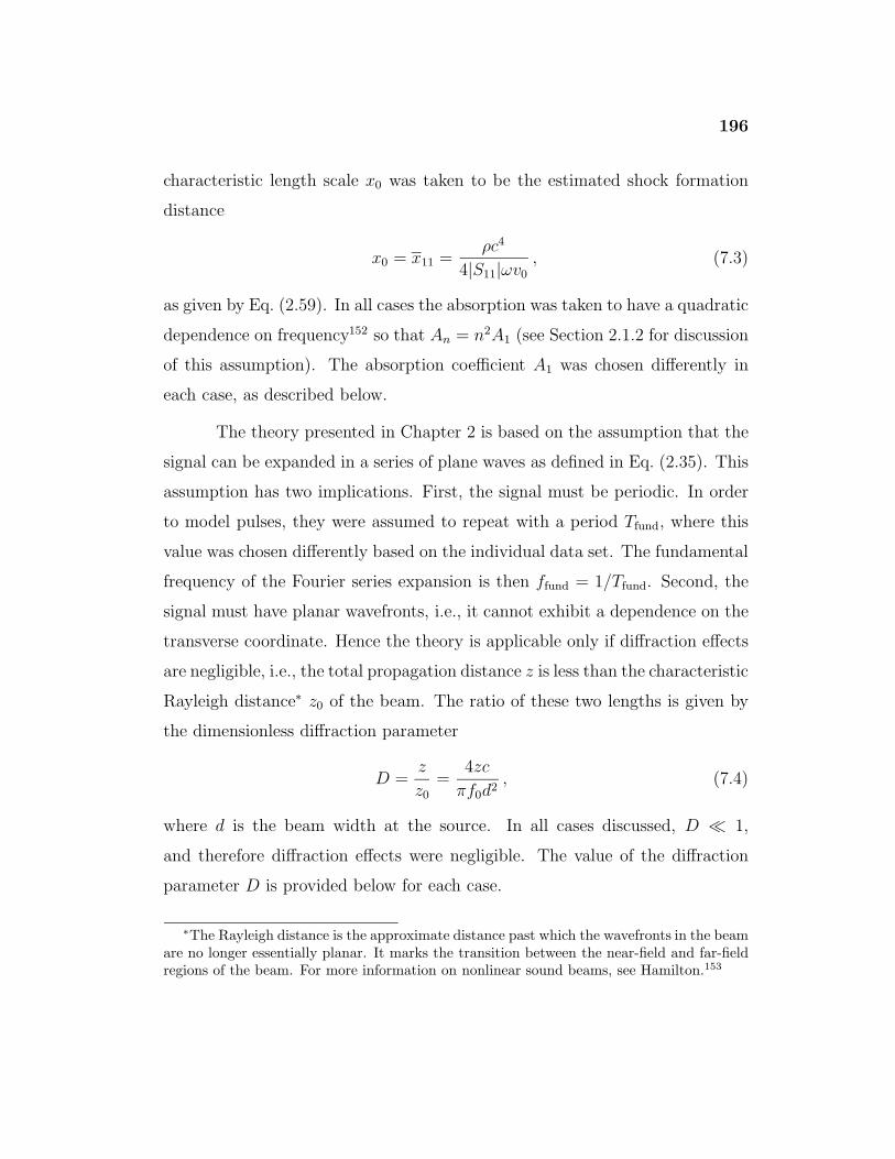
196
characteristic length scale x0 was taken to be the estimated shock formation
distance
x0 = x11 =ρc4
4|S11|ωv0, (7.3)
as given by Eq. (2.59). In all cases the absorption was taken to have a quadratic
dependence on frequency152 so that An = n2A1 (see Section 2.1.2 for discussion
of this assumption). The absorption coefficient A1 was chosen differently in
each case, as described below.
The theory presented in Chapter 2 is based on the assumption that the
signal can be expanded in a series of plane waves as defined in Eq. (2.35). This
assumption has two implications. First, the signal must be periodic. In order
to model pulses, they were assumed to repeat with a period Tfund, where this
value was chosen differently based on the individual data set. The fundamental
frequency of the Fourier series expansion is then ffund = 1/Tfund. Second, the
signal must have planar wavefronts, i.e., it cannot exhibit a dependence on the
transverse coordinate. Hence the theory is applicable only if diffraction effects
are negligible, i.e., the total propagation distance z is less than the characteristic
Rayleigh distance∗ z0 of the beam. The ratio of these two lengths is given by
the dimensionless diffraction parameter
D =z
z0=
4zc
πf0d2, (7.4)
where d is the beam width at the source. In all cases discussed, D � 1,
and therefore diffraction effects were negligible. The value of the diffraction
parameter D is provided below for each case.
∗The Rayleigh distance is the approximate distance past which the wavefronts in the beamare no longer essentially planar. It marks the transition between the near-field and far-fieldregions of the beam. For more information on nonlinear sound beams, see Hamilton.153
197
With the assumptions of the theory satisfied, the evolution equations
were then integrated numerically using a fixed step size, fourth-order Runge–
Kutta routine. Several parameters may be varied in the integration routines
including the number of harmonics, step size, and absorption. The frequency
spectra were truncated between N = 400 and N = 1200 harmonics. Because
the pulses are initially broadband, a larger number of harmonics must be used
than with monofrequency waves (N = 200) to minimize errors associated with
the truncation of the spectrum. A smaller number of harmonics is desirable
because computation time is proportional to N2; however, too few harmonics
can introduce spurious oscillations in the waveforms or cause numerical insta-
bility. (Note that the number of harmonics listed in the tables below is not
necessarily the minimum number possible to gain accurate results.) The di-
mensionless step size of the integration was taken to be between ∆X = 0.0001
and ∆X = 0.0005. By trial and error, this range was found to maintain nu-
merical stability while minimizing computation time. Typically, stability was
also enhanced by using a smaller step size ∆Xinit in the region 0 ≤ X ≤ Xswitch
near the source, and then switching to a larger values of ∆X for the rest of the
integration. A suitable value of Xswitch was found to be approximately where
the Nth harmonic achieved its maximum value after the initial spread of energy
over the entire spectral range. Finally, the absorption coefficient A1 was usually
chosen to be as small as possible to maintain numerical stability and provide
reasonable computation time. Because the quadratic dependence of absorp-
tion on frequency implies that most of the energy is dissipated at the highest
harmonics, integrating with lower absorption requires using a larger number of
harmonics which, in turn, quadratically increases computation time. All the
numerical parameters used for the integration are provided below for each case.
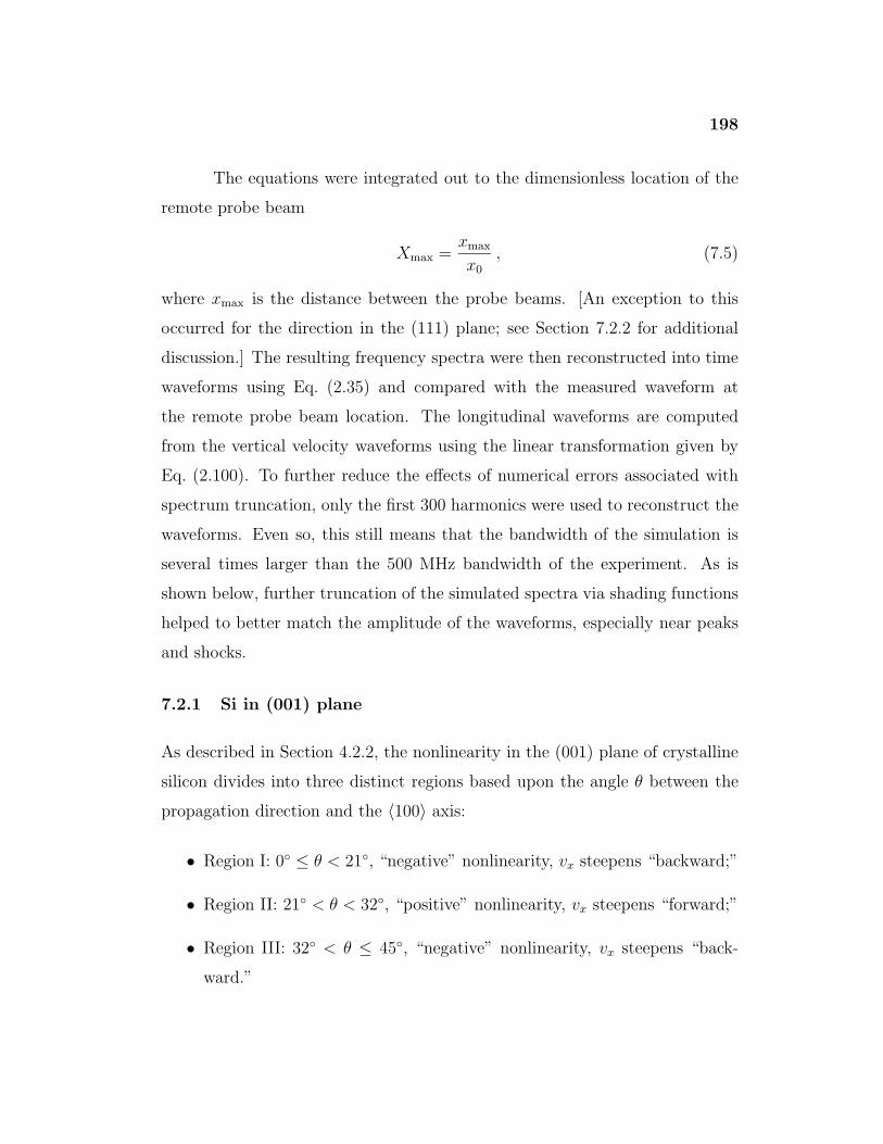
198
The equations were integrated out to the dimensionless location of the
remote probe beam
Xmax =xmax
x0
, (7.5)
where xmax is the distance between the probe beams. [An exception to this
occurred for the direction in the (111) plane; see Section 7.2.2 for additional
discussion.] The resulting frequency spectra were then reconstructed into time
waveforms using Eq. (2.35) and compared with the measured waveform at
the remote probe beam location. The longitudinal waveforms are computed
from the vertical velocity waveforms using the linear transformation given by
Eq. (2.100). To further reduce the effects of numerical errors associated with
spectrum truncation, only the first 300 harmonics were used to reconstruct the
waveforms. Even so, this still means that the bandwidth of the simulation is
several times larger than the 500 MHz bandwidth of the experiment. As is
shown below, further truncation of the simulated spectra via shading functions
helped to better match the amplitude of the waveforms, especially near peaks
and shocks.
7.2.1 Si in (001) plane
As described in Section 4.2.2, the nonlinearity in the (001) plane of crystalline
silicon divides into three distinct regions based upon the angle θ between the
propagation direction and the 〈100〉 axis:
• Region I: 0◦ ≤ θ < 21◦, “negative” nonlinearity, vx steepens “backward;”
• Region II: 21◦ < θ < 32◦, “positive” nonlinearity, vx steepens “forward;”
• Region III: 32◦ < θ ≤ 45◦, “negative” nonlinearity, vx steepens “back-
ward.”
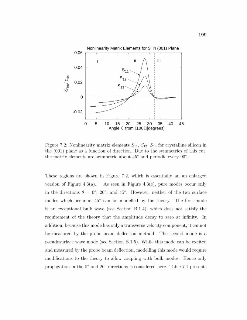
199
-0.02
0
0.02
0.04
0.06
0 5 10 15 20 25 30 35 40 45
S
S
S-S
/
c
13
12
1144
lm
Angle θ from [degrees]⟨100 ⟩
Nonlinearity Matrix Elements for Si in (001) Plane
I II III
Figure 7.2: Nonlinearity matrix elements S11, S12, S13 for crystalline silicon inthe (001) plane as a function of direction. Due to the symmetries of this cut,the matrix elements are symmetric about 45◦ and periodic every 90◦.
These regions are shown in Figure 7.2, which is essentially an an enlarged
version of Figure 4.3(a). As seen in Figure 4.3(e), pure modes occur only
in the directions θ = 0◦, 26◦, and 45◦. However, neither of the two surface
modes which occur at 45◦ can be modelled by the theory. The first mode
is an exceptional bulk wave (see Section B.1.4), which does not satisfy the
requirement of the theory that the amplitude decay to zero at infinity. In
addition, because this mode has only a transverse velocity component, it cannot
be measured by the probe beam deflection method. The second mode is a
pseudosurface wave mode (see Section B.1.5). While this mode can be excited
and measured by the probe beam deflection, modelling this mode would require
modifications to the theory to allow coupling with bulk modes. Hence only
propagation in the 0◦ and 26◦ directions is considered here. Table 7.1 presents
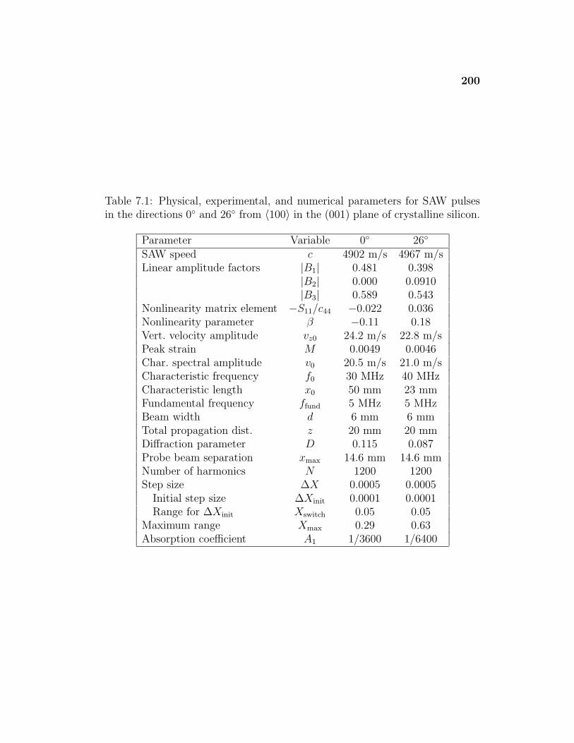
200
Table 7.1: Physical, experimental, and numerical parameters for SAW pulsesin the directions 0◦ and 26◦ from 〈100〉 in the (001) plane of crystalline silicon.
Parameter Variable 0◦ 26◦
SAW speed c 4902 m/s 4967 m/sLinear amplitude factors |B1| 0.481 0.398
|B2| 0.000 0.0910|B3| 0.589 0.543
Nonlinearity matrix element −S11/c44 −0.022 0.036Nonlinearity parameter β −0.11 0.18Vert. velocity amplitude vz0 24.2 m/s 22.8 m/sPeak strain M 0.0049 0.0046Char. spectral amplitude v0 20.5 m/s 21.0 m/sCharacteristic frequency f0 30 MHz 40 MHzCharacteristic length x0 50 mm 23 mmFundamental frequency ffund 5 MHz 5 MHzBeam width d 6 mm 6 mmTotal propagation dist. z 20 mm 20 mmDiffraction parameter D 0.115 0.087Probe beam separation xmax 14.6 mm 14.6 mmNumber of harmonics N 1200 1200Step size ∆X 0.0005 0.0005
Initial step size ∆Xinit 0.0001 0.0001Range for ∆Xinit Xswitch 0.05 0.05
Maximum range Xmax 0.29 0.63Absorption coefficient A1 1/3600 1/6400
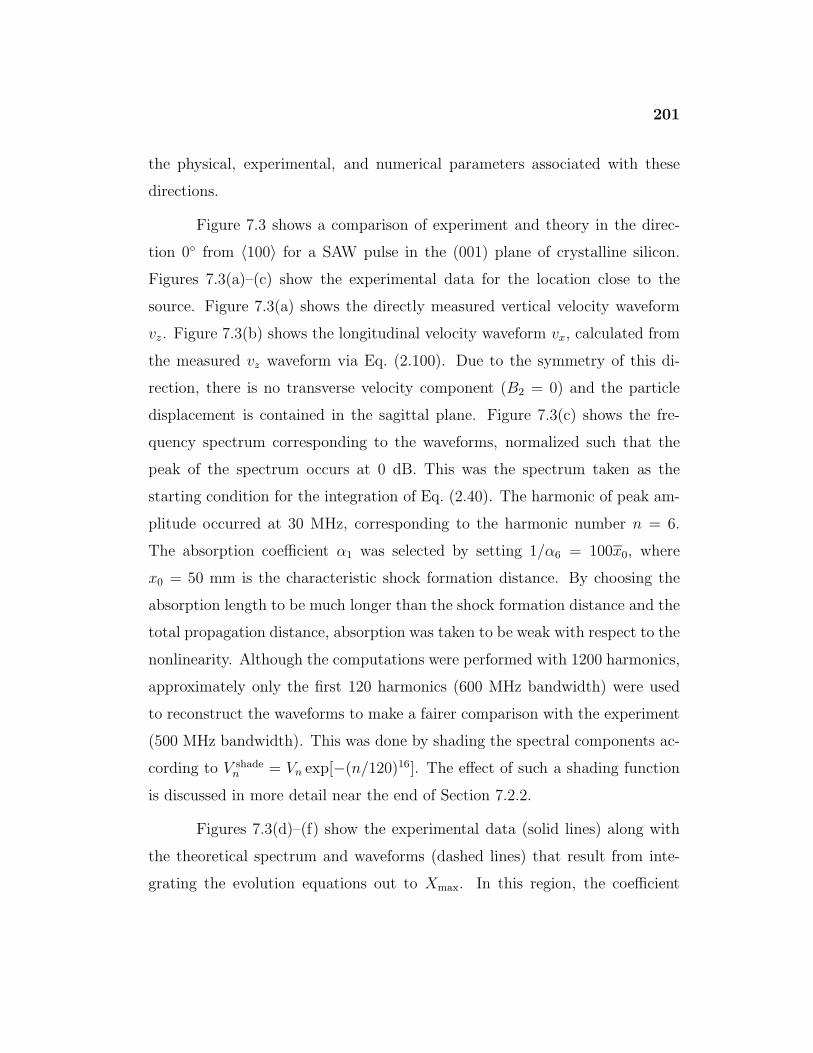
201
the physical, experimental, and numerical parameters associated with these
directions.
Figure 7.3 shows a comparison of experiment and theory in the direc-
tion 0◦ from 〈100〉 for a SAW pulse in the (001) plane of crystalline silicon.
Figures 7.3(a)–(c) show the experimental data for the location close to the
source. Figure 7.3(a) shows the directly measured vertical velocity waveform
vz. Figure 7.3(b) shows the longitudinal velocity waveform vx, calculated from
the measured vz waveform via Eq. (2.100). Due to the symmetry of this di-
rection, there is no transverse velocity component (B2 = 0) and the particle
displacement is contained in the sagittal plane. Figure 7.3(c) shows the fre-
quency spectrum corresponding to the waveforms, normalized such that the
peak of the spectrum occurs at 0 dB. This was the spectrum taken as the
starting condition for the integration of Eq. (2.40). The harmonic of peak am-
plitude occurred at 30 MHz, corresponding to the harmonic number n = 6.
The absorption coefficient α1 was selected by setting 1/α6 = 100x0, where
x0 = 50 mm is the characteristic shock formation distance. By choosing the
absorption length to be much longer than the shock formation distance and the
total propagation distance, absorption was taken to be weak with respect to the
nonlinearity. Although the computations were performed with 1200 harmonics,
approximately only the first 120 harmonics (600 MHz bandwidth) were used
to reconstruct the waveforms to make a fairer comparison with the experiment
(500 MHz bandwidth). This was done by shading the spectral components ac-
cording to V shaden = Vn exp[−(n/120)16]. The effect of such a shading function
is discussed in more detail near the end of Section 7.2.2.
Figures 7.3(d)–(f) show the experimental data (solid lines) along with
the theoretical spectrum and waveforms (dashed lines) that result from inte-
grating the evolution equations out to Xmax. In this region, the coefficient
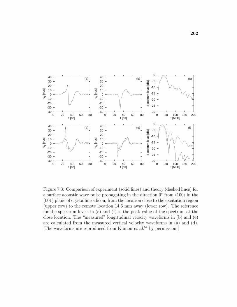
202
-40-30-20-10
010203040
0 20 40 60 80
v z [m
/s]
t [ns]
(a)
-40-30-20-10
010203040
0 20 40 60 80
v z [m
/s]
t [ns]
(d)
-40-30-20-10
010203040
0 20 40 60 80
v x [m
/s]
t [ns]
(b)
-40-30-20-10
010203040
0 20 40 60 80
v x [m
/s]
t [ns]
(e)
-30
-25
-20
-15
-10
-5
0
0 50 100 150 200
Spe
ctru
m le
vel [
dB]
f [MHz]
(c)
-30
-25
-20
-15
-10
-5
0
0 50 100 150 200
Spe
ctru
m le
vel [
dB]
f [MHz]
(f)
Figure 7.3: Comparison of experiment (solid lines) and theory (dashed lines) fora surface acoustic wave pulse propagating in the direction 0◦ from 〈100〉 in the(001) plane of crystalline silicon, from the location close to the excitation region(upper row) to the remote location 14.6 mm away (lower row). The referencefor the spectrum levels in (c) and (f) is the peak value of the spectrum at theclose location. The “measured” longitudinal velocity waveforms in (b) and (e)are calculated from the measured vertical velocity waveforms in (a) and (d).[The waveforms are reproduced from Kumon et al.54 by permission.]
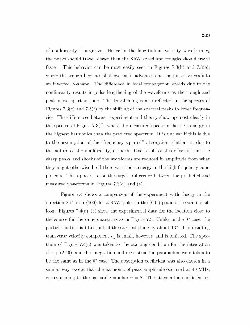
203
of nonlinearity is negative. Hence in the longitudinal velocity waveform vx
the peaks should travel slower than the SAW speed and troughs should travel
faster. This behavior can be most easily seen in Figures 7.3(b) and 7.3(e),
where the trough becomes shallower as it advances and the pulse evolves into
an inverted N-shape. The difference in local propagation speeds due to the
nonlinearity results in pulse lengthening of the waveforms as the trough and
peak move apart in time. The lengthening is also reflected in the spectra of
Figures 7.3(c) and 7.3(f) by the shifting of the spectral peaks to lower frequen-
cies. The differences between experiment and theory show up most clearly in
the spectra of Figure 7.3(f), where the measured spectrum has less energy in
the highest harmonics than the predicted spectrum. It is unclear if this is due
to the assumption of the “frequency squared” absorption relation, or due to
the nature of the nonlinearity, or both. One result of this effect is that the
sharp peaks and shocks of the waveforms are reduced in amplitude from what
they might otherwise be if there were more energy in the high frequency com-
ponents. This appears to be the largest difference between the predicted and
measured waveforms in Figures 7.3(d) and (e).
Figure 7.4 shows a comparison of the experiment with theory in the
direction 26◦ from 〈100〉 for a SAW pulse in the (001) plane of crystalline sil-
icon. Figures 7.4(a)–(c) show the experimental data for the location close to
the source for the same quantities as in Figure 7.3. Unlike in the 0◦ case, the
particle motion is tilted out of the sagittal plane by about 13◦. The resulting
transverse velocity component vy is small, however, and is omitted. The spec-
trum of Figure 7.4(c) was taken as the starting condition for the integration
of Eq. (2.40), and the integration and reconstruction parameters were taken to
be the same as in the 0◦ case. The absorption coefficient was also chosen in a
similar way except that the harmonic of peak amplitude occurred at 40 MHz,
corresponding to the harmonic number n = 8. The attenuation coefficient α1
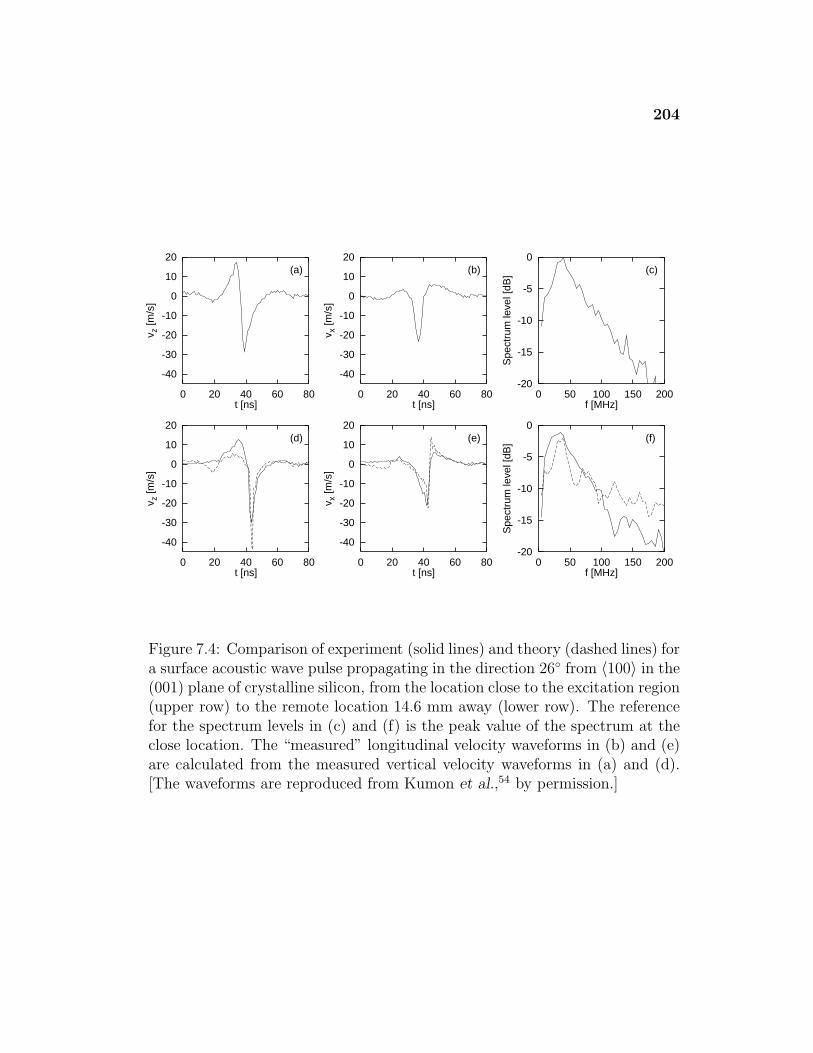
204
-40
-30
-20
-10
0
10
20
0 20 40 60 80
v z [m
/s]
t [ns]
(a)
-40
-30
-20
-10
0
10
20
0 20 40 60 80
v z [m
/s]
t [ns]
(d)
-40
-30
-20
-10
0
10
20
0 20 40 60 80
v x [m
/s]
t [ns]
(b)
-40
-30
-20
-10
0
10
20
0 20 40 60 80
v x [m
/s]
t [ns]
(e)
-20
-15
-10
-5
0
0 50 100 150 200
Spe
ctru
m le
vel [
dB]
f [MHz]
(c)
-20
-15
-10
-5
0
0 50 100 150 200
Spe
ctru
m le
vel [
dB]
f [MHz]
(f)
Figure 7.4: Comparison of experiment (solid lines) and theory (dashed lines) fora surface acoustic wave pulse propagating in the direction 26◦ from 〈100〉 in the(001) plane of crystalline silicon, from the location close to the excitation region(upper row) to the remote location 14.6 mm away (lower row). The referencefor the spectrum levels in (c) and (f) is the peak value of the spectrum at theclose location. The “measured” longitudinal velocity waveforms in (b) and (e)are calculated from the measured vertical velocity waveforms in (a) and (d).[The waveforms are reproduced from Kumon et al.,54 by permission.]
205
was selected by setting 1/α8 = 100x0, where x0 = 23 mm is the characteristic
shock formation distance.
The predicted frequency spectra and waveforms (dashed lines) are com-
pared with the measurements (solid lines) in Figure 7.4(d)–(f). In this region,
the coefficient of nonlinearity is positive. Hence in the longitudinal velocity
vx the peaks should travel faster than the SAW speed and troughs should
travel slower. This behavior can probably be most easily seen in Figures 7.4(b)
and 7.4(e), where the blunter positive peaks evolve into the sharper positive
peaks. The nonlinearity causes the waveforms to develop into a sawtooth shape
like in a fluid, except for the cusping near the shock front. In addition, pos-
itive nonlinearity causes negative peaks of the vertical velocity vz to become
more negative, as seen in Figures 7.4(a) and 7.4(d). The differences between
experiment and theory show up most clearly in the spectra in Figure 7.4(f).
The decrease in the peak amplitude from its value in Figure 7.4(f) is due to
a combination of energy transfer to higher harmonics and a small amount of
absorption. However, the measured spectrum has less energy in the highest
harmonics than the predicted spectrum, and it also does not exhibit the same
distinct peaks. As in the 0◦ case, it is unclear if this is due to the assump-
tion of the “frequency squared” absorption relation or due to the nature of the
nonlinearity or both.
In summary, the results demonstrate that the theory is corroborated
by the experiment in the 0◦ direction of Region I and the 26◦ direction of
Region II in terms of both the qualitative behavior and quantitative agreement
of the waveforms. It is striking that while the waveforms measured at the close
locations in the 0◦ and 26◦ directions are initially similar in form, they evolve
to waveforms that are significantly different. This is consistent with the regions
of “positive” and “negative” nonlinearity delineated in Figure 7.2.
206
7.2.2 Si in (111) plane
Next consider propagation of SAW pulses in the (111) plane of crystalline
silicon. Figure 6.9(e) shows that only the 0◦ and 30◦ directions are pure modes.
Of these two directions, Figure 6.9(a) shows that the effect of nonlinearity is
approximately an order of magnitude higher in the 0◦ direction than in the 30◦
direction. Note also that the magnitudes of the nonlinearity matrix element
|S11|/c44 and nonlinearity coefficient |β| are several times larger as compared
to the 0◦ and 26◦ directions of the (001) plane. Figure 6.9(b) shows that
the phases of the first few nonlinearity matrix elements are in the vicinity of
106◦ and are relatively close together. As demonstrated for monofrequency
source conditions, this complex-valued nonlinearity results in the asymmetric
distortion of the velocity waveforms, as seen in Figure 6.10. The combination of
heightened nonlinearity and asymmetric distortion should result in significantly
different waveforms than observed in the (001) plane.
Figure 7.5 provides a comparison of the experiment with theory for a
SAW pulse in the (111) plane of crystalline silicon in the direction 0◦ from
〈112〉. As seen in Figure 6.10(g), the wave has no transverse velocity compo-
nent (B2 = 0), and hence only the vertical and longitudinal components are
shown in Figure 7.5. Figures 7.5(a)–(c) display the measured waveforms and
spectrum at distance x = 5 mm from the excitation region. As before, the lon-
gitudinal velocity waveforms are computed from the vertical velocity waveforms
using Eq. (2.100). Figure 7.5(c) shows the corresponding frequency spectrum
that was used as the starting condition for the integration of Eq. (2.40). The
spectrum is normalized so that its peak at 50 MHz occurs has an amplitude
of 0 dB. The absorption coefficient was chosen so that 1/α1 = 40x0 where
x0 = 2.9 mm is the characteristic shock formation distance. The computa-
tions were performed with 400 harmonics, although only the first 70 harmonics
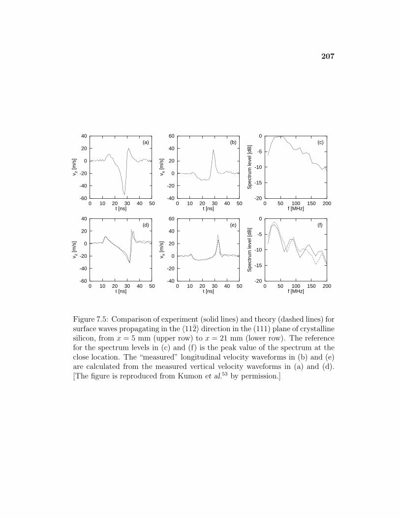
207
-60
-40
-20
0
20
40
0 10 20 30 40 50
v z [m
/s]
t [ns]
(a)
-60
-40
-20
0
20
40
0 10 20 30 40 50
v z [m
/s]
t [ns]
(d)
-40
-20
0
20
40
60
0 10 20 30 40 50
v x [m
/s]
t [ns]
(b)
-40
-20
0
20
40
60
0 10 20 30 40 50
v x [m
/s]
t [ns]
(e)
-20
-15
-10
-5
0
0 50 100 150 200
Spe
ctru
m le
vel [
dB]
f [MHz]
(c)
-20
-15
-10
-5
0
0 50 100 150 200
Spe
ctru
m le
vel [
dB]
f [MHz]
(f)
Figure 7.5: Comparison of experiment (solid lines) and theory (dashed lines) forsurface waves propagating in the 〈112〉 direction in the (111) plane of crystallinesilicon, from x = 5 mm (upper row) to x = 21 mm (lower row). The referencefor the spectrum levels in (c) and (f) is the peak value of the spectrum at theclose location. The “measured” longitudinal velocity waveforms in (b) and (e)are calculated from the measured vertical velocity waveforms in (a) and (d).[The figure is reproduced from Kumon et al.53 by permission.]
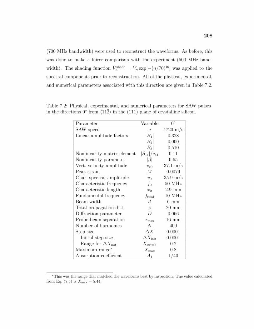
208
(700 MHz bandwidth) were used to reconstruct the waveforms. As before, this
was done to make a fairer comparison with the experiment (500 MHz band-
width). The shading function V shaden = Vn exp[−(n/70)16] was applied to the
spectral components prior to reconstruction. All of the physical, experimental,
and numerical parameters associated with this direction are given in Table 7.2.
Table 7.2: Physical, experimental, and numerical parameters for SAW pulsesin the directions 0◦ from 〈112〉 in the (111) plane of crystalline silicon.
Parameter Variable 0◦
SAW speed c 4720 m/sLinear amplitude factors |B1| 0.328
|B2| 0.000|B3| 0.510
Nonlinearity matrix element |S11|/c44 0.11Nonlinearity parameter |β| 0.65Vert. velocity amplitude vz0 37.1 m/sPeak strain M 0.0079Char. spectral amplitude v0 35.9 m/sCharacteristic frequency f0 50 MHzCharacteristic length x0 2.9 mmFundamental frequency ffund 10 MHzBeam width d 6 mmTotal propagation dist. z 20 mmDiffraction parameter D 0.066Probe beam separation xmax 16 mmNumber of harmonics N 400Step size ∆X 0.0001
Initial step size ∆Xinit 0.0001Range for ∆Xinit Xswitch 0.2
Maximum range∗ Xmax 0.8Absorption coefficient A1 1/40
∗This was the range that matched the waveforms best by inspection. The value calculatedfrom Eq. (7.5) is Xmax = 5.44.
209
Figures 7.5(d)–(f) show the measurements (solid lines) compared with
the calculations (dashed lines) for the frequency spectrum and waveforms that
result from integrating the evolution equations out to Xmax = 0.8. This value
was chosen by inspecting the theoretical waveforms after various propagation
distances to determine the one that best fits the experimental data. Unfortu-
nately, the value Xmax = 5.44 predicted by Eq. (7.5) appears to significantly
overestimate the characteristic nonlinear length scale. The cause of this dis-
crepancy is not clear, although it may be related to the more complicated
nature of the waveform distortion that results from complex-valued nonlinear-
ity matrix elements. Note, however, that no other parameters were varied to
achieve these results, other than the ending location of the integration. Despite
this scaling problem, the measured waveforms and spectra are reproduced well
at the remote location, as shown in Figure 7.5(d)–(f). The nonlinear waveform
distortion is predicted accurately by the theory, including the increase in pulse
duration between the close and remote locations. The lengthening is mani-
fested in the shift of the spectral peak from 50 MHz down to about 30 MHz.
In addition, there are notable differences in the distortion of the waveform as
compared to measurements of nonlinear Rayleigh waves in fused quartz26 and
the nonlinear SAWs in the (001) plane shown in Section 7.2.1. In the case
shown in Figure 7.5, the vertical component vz has an N-shaped waveform and
the horizontal component vx has a U-shaped waveform, whereas the reverse
was observed in isotropic solids and in the 0◦ direction in the (001) plane of
silicon. The case shown in Figure 7.5 also differs from the 26◦ direction in the
(001) plane of silicon, where the vz component develops a sharp negative peak
and the vx component develops into a cusped sawtooth wave. Nevertheless, the
evolution of the waveforms is consistent with the distortion seen in the initially
monofrequency waveforms of Figure 6.10, which show a shock forming in the
vz waveform and a positive peak and shallow trough forming the vx direction.
210
Hence Figure 6.10 shows that the change of the measured waveforms in the
(111) plane as compared to previous cases in the (001) plane is a direct re-
sult of the approximately 100◦ phase shift induced by the first few nonlinearity
matrix elements.
For the reasons stated above, the predicted frequency spectra shown in
Figures 7.3, 7.4, and 7.5 incorporate shading to better match the bandwidth
of the experiment. To demonstrate the effect of the shading, the longitudinal
velocity waveforms for the 0◦ direction in the (111) plane were reconstructed
(1) with shading to simulate approximately 700 MHz of bandwidth, and (2)
without shading to simulate 3000 MHz of bandwidth. The results are shown in
Figure 7.6. In both cases the simulations were run with a maximum bandwidth
of 4000 MHz (400 harmonics × 10 MHz fundamental frequency). The largest
change in the waveforms is that the peak heightens and narrows, increasing
from around 35 m/s to around 50 m/s. This is not unexpected because adding
additional high frequency information allows steeper shocks and sharper peaks
to be resolved. The exact form of the exponential shading profile shown in Fig-
ure 7.6 was selected to provide a rapidly decaying function that was not discon-
tinuous. Trials with other functions that retained roughly the same amount of
frequency content (including a step function) were found to cause relatively lit-
tle change in the shape of the reconstructed waveforms. However, reducing the
effective bandwidth further (even as high as 500 MHz) was found to introduce
excessively blunt peaks and overemphasize low frequency oscillations. One pos-
sible conclusion from this result is that an experiment with higher bandwidth
capabilities may measure even larger peaks and steeper shocks than seen in the
experimental waveforms in this chapter.
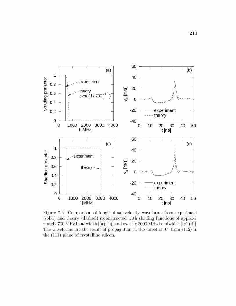
211
0
0
0.2
0.2
0.4
0.4
0.6
0.6
0.8
0.8
1
1
0
0
1000
1000
2000
2000
3000
3000
4000
4000
Sha
ding
pre
fact
orS
hadi
ng p
refa
ctor
f [MHz]
f [MHz]
-40
-40
-20
-20
0
0
20
20
40
40
60
60
0
0
10
10
20
20
30
30
40
40
50
50
vv
xx
[m/s
] [m
/s]
t [ns]
t [ns]
(c) (d)
(b)(a)
theory
experiment
exp(-[ f / 700 ]16 )
experimenttheory
experiment
theory
experimenttheory
Figure 7.6: Comparison of longitudinal velocity waveforms from experiment(solid) and theory (dashed) reconstructed with shading functions of approxi-mately 700 MHz bandwidth [(a),(b)] and exactly 3000 MHz bandwidth [(c),(d)].The waveforms are the result of propagation in the direction 0◦ from 〈112〉 inthe (111) plane of crystalline silicon.
212
7.3 Summary
This chapter has discussed nonlinear SAW pulses, specifically focusing on prop-
agation in crystalline silicon. Through collaboration with an experimental
group,53,54 measurements were obtained for the directions 0◦ and 26◦ from
〈100〉 in the (001) plane and the direction 0◦ from 〈112〉 in the (111) plane.
The photoelastic technique developed by Lomonosov, Mikhalevich, and Hess
for the generation and detection of nonlinear SAWs is described. In addition,
the procedure used to perform the numerical analysis of their measurements is
reviewed in detail. In all cases, favorable agreement is achieved between exper-
iment and theory. In the (001) plane, the pulses corroborate the notion that
there exist regions of directions with “positive” and “negative” nonlinearity. In
the (111) plane, the waveform distortion is consistent with the phase changes
associated with the predicted complex-valued nonlinearity matrix elements.
Hopefully, further experimental studies will be performed to investigate the
broad range of phenomena that have been proposed to exist in the propagation
of nonlinear SAWs in cubic crystals.
Chapter 8
Summary
This dissertation has undertaken a comprehensive study of nonlinear surface
acoustic waves (SAWs) in nonpiezoelectric cubic crystals based on the theory
developed by Hamilton, Il’inskii, and Zabolotskaya33 for anisotropic media. A
review of the literature reveals that very few simulations of the fully nonlinear
evolution of SAWs have been reported. The reported cases describe only a few
selected materials and particular directions of high symmetry. Moreover, no
work had presented a comparison of experiment and theory for the evolution
of nonlinear SAW waveforms in crystals. Hence the goal of this work was
to use the aforementioned theory to characterize and explain the nature of
the harmonic generation and waveform distortion of nonlinear SAWs over a
wide variety of directions, cuts, and materials, and to validate these results by
comparison with experiment.
Chapter 2 began by outlining the theory of Hamilton, Il’inskii, and
Zabolotskaya.33 By using a Hamiltonian mechanics approach, they derived a
set of frequency-domain model equations to describe the evolution of SAWs in
arbitrary directions and cuts of crystalline media of any symmetry. Quasilin-
ear solutions were derived for these evolution equations under several different
approximations. Via analogy to nonlinear bulk wave propagation in fluids and
solids, expressions were derived for estimates of the shock formation distance
and nonlinearity coefficient. A time-domain evolution equation was developed
from the frequency-domain equations and was shown to reduce to the time-
213
214
domain evolution equation for nonlinear Rayleigh waves20 in the isotropic limit.
Finally, a detailed comparison was made between the various papers derived
from the theory of Zabolotskaya for nonlinear Rayleigh waves and the afore-
mentioned theory for anisotropic media.
Chapter 3 reviewed briefly the basic properties of cubic crystals. Cubic
crystals were chosen for study because they have the highest symmetry of all
crystalline classes and, therefore, the simplest type of fully three-dimensional
anisotropy. In addition, previous investigations have shown that effects exhib-
ited in cubic crystals are often similar to those seen in other crystal types. A set
of tables was given that compiled the measured densities, second-order elastic
constants, and third-order elastic constants for all the materials modelled in
the dissertation.
Chapters 4 and 5 studied the properties of initially monofrequency non-
linear SAWs in the (001) and (110) planes, respectively. Fifteen crystals were
selected for study, including RbCl, KCl, NaCl, CaF2, SrF2, BaF2, C (diamond),
Si, Ge, Al, Ni, Cu in the m3m point group, and Cs-alum, NH4-alum, and K-
alum in the m3 point group [the hydrous X-alums have the chemical formulas
XAl(SO4)2 · 12 H2O]. Si, KCl, and Ni were chosen for study in detail. The mag-
nitudes of the nonlinearity matrix elements were shown to provide a powerful
tool for characterizing the nature of the waveform evolution in these planes.
In most crystals, these elements were demonstrated to be a strong function of
propagation direction. Several interesting effects were found in common, in-
cluding (1) propagation directions in which the nature of the velocity waveform
distortion changes in sign, (2) directions in which the generation of one or more
harmonics are suppressed, thereby causing little or no shock formation, and (3)
directions in which energy is rapidly transferred to the highest harmonics and
shock formation is enhanced. In all cases except the (110) plane of crystals in
215
the m3 point group, the nonlinearity matrix elements were shown to be real-
valued. The choice of different experimental TOE constants as input to the
simulations is shown to affect the detailed predictions of the nonlinearity ma-
trix elements in any given direction, but not the trends over the whole angular
range.
Chapter 6 studied the properties of initially monofrequency nonlinear
SAWs in the (111) plane. For all fifteen crystals studied, the nonlinearity ma-
trix elements are complex-valued. Both the magnitude and phase of the ma-
trix elements were considered to explain the waveform evolution. The relative
phases of the dominant nonlinearity matrix elements were shown to be partic-
ularly important. The phasing produces waveform distortion that is generally
asymmetric, and it can lead to a nonlinear dispersion-like effect whereby low
frequency oscillations form near the peaks and shocks in the velocity waveforms.
A novel interpretation of complex-valued nonlinearity matrices was proposed
and shown to provide a simple method for characterizing the type of waveform
distortion, especially when the dominant nonlinearity matrix elements have
similar phases.
Chapter 7 described the modelling of SAW pulses in crystalline silicon
and compared numerical simulations to experiment. Through a collaboration
with A. Lomonosov, V. G. Mikhalevich, and P. Hess, measurements were ob-
tained with nonlinear SAW pulses in the directions 0◦ and 26◦ from 〈100〉 in the
(001) plane and 0◦ from 〈112〉 in the (111) plane of crystalline Si. A brief de-
scription of the photoelastic technique for generating and measuring the SAWs
was given, followed by a discussion of the numerical analysis of the data. In the
(001) plane, it was found that the measurements validated the predictions of
the theory that there exist regions of “positive” and “negative” nonlinearity as
a function of propagation direction. In the (111) plane, the type of waveform
216
distortion was found to be reversed between the vertical and longitudinal direc-
tions. This result is consistent with the phases of the predicted complex-valued
nonlinearity matrix elements for this case.
Finally, several appendices were provided on auxiliary topics, including
a discussion of the terms “anisotropy” and “aeolotropy,” a tutorial on the basic
properties of linear and nonlinear SAWs in crystals, a review of many appli-
cations of linear and nonlinear SAWs, a description of Miller index notation,
a detailed derivation of the time-domain relation between the velocity compo-
nents of a SAW in a crystal, and additional discussion about the interpretation
of complex-valued nonlinearity parameters.
Future theoretical work in this area will probably include modelling
nonlinear SAW propagation in non-cubic crystals, using an extension of the
theory to study propagation in a variety of piezoelectric crystals, and extending
both theories to include dispersion (e.g., introduced by a thin layer on the
surface of the material) and diffraction. It is hoped that future experimental
work will further validate many of the properties of SAWs presented in this
work.
Appendix A
Anisotropic and Aeolotropic Media
In some texts, a distinction is made between anisotropic and aeolotropic media.
According to Smith and Stephens,154
These two words are often used synonymously in the literature, but
more specifically the term aeolotropic is used in connection with
materials possessing no internal boundaries such as single crystals,
while the term anisotropic is concerned with the bulk properties.
A polycrystalline aggregate in which there is partial alignment of
the individual ‘aeolotropic’ single crystal grains would exhibit ‘ani-
sotropic’ bulk properties, but a randomly oriented aggregate would
show isotropic physical characteristics.
Musgrave113 gives another example:
For example, a cylindrical bar, plastically formed from an aggregate
of crystallites with cubic symmetry may well exhibit preferential
orientation such that directions lying in the circular cross-section
are equivalent but differ from the axial direction. Such a bar is said
to be transversely isotropic and possesses on a macroscopic scale,
the same symmetry as a hexagonal crystal. Thus we see that the
aeolotropy of physical properties implied by the basic structure of
a crystal may be camouflaged or wholly smeared out by preferred
or random orientation.
The theory of Hamilton, Il’inskii, and Zabolotskaya33 used in this dissertation
characterizes completely the investigated media by the specification of the den-
sity and second- and third-order elastic constants. Thus if the elastic constants
217
218
of the medium under consideration reflect the symmetry properties of that
sample, then the nonlinear surface waves generated in the sample are correctly
described by the theory (provided all other assumptions of the theory are met).
For example, consider Musgrave’s example of a bar cut in such a way
that it has a flat surface. It would be incorrect to apply the aforementioned
SAW theory to this sample with elastic constant data for the cubic aeolotropy
of individual crystallites, but it would be appropriate to apply the theory with
elastic constants of hexagonal anisotropy measured from the bulk polycrys-
talline aggregate. Note that the theory could not be applied if the anisotropy
were inhomogeneous (e.g., if the aeolotropy or distribution of the individual
crystallites varied with location in the bar). In most cases considered in this
work, the media are single crystals. In these cases the distinction between ae-
olotropy and anisotropy is not important because the aeolotropy is the same
on both the microscopic and macroscopic scales. Thus the term “anisotropy”
is used exclusively throughout the text as this is consistent with most of the
literature on surface acoustic waves in these types of media.
As might be expected from their similar meaning, the words have a
similar etymology. The word “aeolotropy” comes from the Greek roots αιoλoς+
τρoπια meaning “changeful turning,” while the word “anisotropy” comes from
the Greek roots ανισoς + τρoπια meaning “unequal turning” [Oxford English
Dictionary (Oxford University Press, London, 1933)].
Appendix B
Surface Acoustic Wave Tutorial
Surface acoustic waves can be classified into nondispersive and dispersive waves.
For additional information about the various kinds of SAWs discussed below,
the interested reader may refer to the excellent reviews by Farnell,3,4 Farnell and
Adler,5 Auld,105 Stegeman and Nizzoli,6 Feldmann and Henaff,7 Biryukov et
al.8 in the linear regime and by Parker9 and Mayer10 in the nonlinear regime.
Henceforth, all media considered are assumed to be elastic, i.e., at all times
the internal forces of the medium or stress depend only on the deformation
of the material or strain as measured relative to the undisturbed state. In
addition, the wavelengths of the acoustic waves are assumed to be sufficiently
large compared to the size of the molecules in the material that a continuum
model of the solid is valid. The tutorial focuses primarily on nondispersive
waves, but a short description of dispersive waves is also provided.
B.1 Nondispersive Waves
Nondispersive waves have a wave speed which is independent of their frequency.
Because the nonlinear effects usually occur on a slow time scale in comparison
to the time scale of the wave propagation, significant nonlinear interaction
between the different frequency components or harmonics becomes possible
only when these components propagate together at the same speed. It is this
slow accumulation of effects that gives rise to waveform distortion and shock
formation. The properties of Rayleigh, Stoneley, Scholte, and leaky Rayleigh,
219
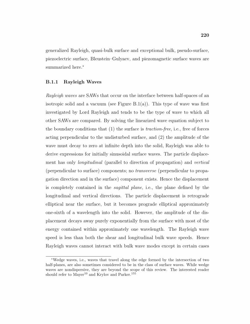
220
generalized Rayleigh, quasi-bulk surface and exceptional bulk, pseudo-surface,
piezoelectric surface, Bleustein–Gulyaev, and piezomagnetic surface waves are
summarized here.∗
B.1.1 Rayleigh Waves
Rayleigh waves are SAWs that occur on the interface between half-spaces of an
isotropic solid and a vacuum (see Figure B.1(a)). This type of wave was first
investigated by Lord Rayleigh and tends to be the type of wave to which all
other SAWs are compared. By solving the linearized wave equation subject to
the boundary conditions that (1) the surface is traction-free, i.e., free of forces
acting perpendicular to the undisturbed surface, and (2) the amplitude of the
wave must decay to zero at infinite depth into the solid, Rayleigh was able to
derive expressions for initially sinusoidal surface waves. The particle displace-
ment has only longitudinal (parallel to direction of propagation) and vertical
(perpendicular to surface) components; no transverse (perpendicular to propa-
gation direction and in the surface) component exists. Hence the displacement
is completely contained in the sagittal plane, i.e., the plane defined by the
longitudinal and vertical directions. The particle displacement is retrograde
elliptical near the surface, but it becomes prograde elliptical approximately
one-sixth of a wavelength into the solid. However, the amplitude of the dis-
placement decays away purely exponentially from the surface with most of the
energy contained within approximately one wavelength. The Rayleigh wave
speed is less than both the shear and longitudinal bulk wave speeds. Hence
Rayleigh waves cannot interact with bulk wave modes except in certain cases
∗Wedge waves, i.e., waves that travel along the edge formed by the intersection of twohalf-planes, are also sometimes considered to be in the class of surface waves. While wedgewaves are nondispersive, they are beyond the scope of this review. The interested readershould refer to Mayer10 and Krylov and Parker.155
221
when there is a discontinuity in the surface boundary condition, e.g., reflection
from a corner.4 Because the dispersion relation has solutions for the mate-
rial parameters of any isotropic solid, Rayleigh waves can exist on the surface
of any such solid. General analytical solutions for the linear Rayleigh wave
problem have been explicitly derived by several authors3,105,107,119,156,157 using
a variety of different approaches. See the book by Viktorov14 for a review of
the early theoretical and experimental work on Rayleigh waves, including many
references to the Russian literature.
In the linear regime where the particle displacements are considered
to be infinitesimally small, the initial waveform propagates across the surface
unchanged. However, when finite amplitude waves propagate, energy is trans-
ferred from lower to higher harmonics and the waveform changes in shape. For
simplicity, consider the case of a nonlinear Rayleigh wave with planar wave-
fronts that has an initially sinusoidal time waveform and propagates through a
weakly absorptive medium like steel.20 For such a wave, the horizontal velocity
waveform at the surface distorts into a sawtooth-like wave but with cusps at
the “corners” of the sawtooth which are larger than the initial amplitude of the
sinusoid. Simultaneously, the vertical velocity waveform at the surface evolves
into a sharply cusped impulse. The cusping is attributed to the fact that the
nonlinearly-generated, higher harmonics penetrate less deeply into the solid.
Hence energy from beneath the surface is transferred upwards to the interface
region thereby making the peak amplitude larger.20 The polarity of the saw-
tooth and impulse are dependent upon material parameters. In the reference
frame that moves along at the Rayleigh wave speed, the peaks of the waveform
advance and the troughs recede (like waveform distortion in a fluid108) for some
materials, while for others the opposite occurs. Eventually, thermal absorption
at the shock causes the amplitude of the wave to diminish and the wave re-
turns to the linear regime. The basic features of nonlinear Rayleigh waves
222
described above turn out to be common to many different kinds of SAWs; see
Section 1.3.1 for a discussion of recent work on nonlinear Rayleigh waves.
B.1.2 Stoneley, Scholte, and Leaky Rayleigh Waves
Stoneley waves158 occur on the interface between half-spaces of two different
solids (see Figure B.1(b)). A dispersion relation may be derived by solving the
linearized wave equation in both materials subject to the boundary conditions
that (1) the two solids are bonded such that the particle displacements and
tractions are continuous across the interface and (2) the amplitudes of the waves
in the solids decay to zero at infinite depth into each half-space. However, this
dispersion relation does not necessarily have a solution for any combination
of material parameters; in fact, existence is usually the exception and not the
rule.159–161 This result has been shown in both the cases of isotropic solids27 and
anisotropic solids.162,163 However, whenever there is a solution, that solution
is unique.164 The Stoneley wave speed is always less than the lowest bulk
wave speed in either solid27 but greater than or equal to the slower of two
Rayleigh wave speeds of either solid alone.163 In the case that both materials
are isotropic, the particle displacement in one solid is typically elliptical at the
interface but changes its direction of rotation inside, while in the the other
solid the displacement is elliptical all the way into the half-space. In addition,
the displacement is strictly contained to the sagittal plane. See Meegan27 for
further discussion of Stoneley waves in the linear regime.
Scholte waves165 and leaky Rayleigh waves occur on the interface be-
tween half-spaces of a solid and a fluid (see Figure B.2). They can be consid-
ered to be a limiting case of Stoneley waves when the shear modulus of one of
the media goes to zero. A dispersion relation may be derived by solving the
linearized wave equation in both materials subject to the boundary conditions

223
k
x
k
x
z
Solid
∼λ
z
z/λe
Solid
SolidR
(a) Rayleigh Wave (b) Stoneley Wave
∼λ
z/λe
S
Figure B.1: Schematic representations of a (a) Rayleigh wave and (b) Stoneleywave. [originally Figs. 2.11 and 2.4 from Meegan,27 reproduced by permission].
k
x
z
(a) Scholte Wave
∼ λ
z/λe
-z/λe
z/λeSc k
x
z
SolidSolid
FluidFluid
(b) Leaky Rayleigh Wave
∼ λ
z/λe
lR
Figure B.2: Schematic representations of a (a) Scholte wave and (b) LeakyRayleigh wave. [originally Fig. 2.7 from Meegan,27 reproduced by permission].
224
that (1) the vertical components of the particle displacements are zero at the
interface, (2) the shear stress in the solid is zero at the interface, (3) the per-
pendicular stresses are continuous across the interface, and (4) the amplitudes
of the waves in both media decay to zero at infinite depth into each half-space.
In the case that a root of the dispersion relation is real, then the solution is
called a Scholte wave. For Scholte waves, the particle displacement is retro-
grade elliptical at the surface but becomes prograde elliptical into the solid,
while in the fluid the displacement is retrograde elliptical all the way into the
half-space. In both media, the amplitude of the displacement decays away ex-
ponentially away from the interface. In the case that the root is complex, then
the solution is called a leaky Rayleigh wave. For this case, the amplitude of the
wave in the solid decays exponentially not only into the solid but also in the
direction of propagation. The wave is attenuated in the direction of propaga-
tion because the energy is radiated into the fluid. Accordingly, the amplitude
of the wave in the liquid grows exponentially away from the interface. The
shape of the particle displacement is similar to Scholte waves except that the
elliptical displacement is tilted towards the direction of power flow out of the
solid. A review of some of the earliest work along with a coordinated experi-
mental and theoretical investigation of linear Scholte and leaky Rayleigh waves
(called “Stoneley-like” and “pseudo-Rayleigh waves” in the paper) was per-
formed by Roever, Vining, and Strick.166 More recently Meegan27 performed
an extensive theoretical study of the behavior and existence of linear Scholte
and leaky Rayleigh waves in isotropic solids. In contrast to the Stoneley wave
case, there always exists a solution to the dispersion relation for Scholte waves.
However, leaky Rayleigh waves only exist for certain combinations of material
parameters. In the same work, Meegan also reported that under circumstances
where the interface region is insonified, a “doubly leaky” wave may propagate
along the interface region with energy radiating into both the liquid and solid.
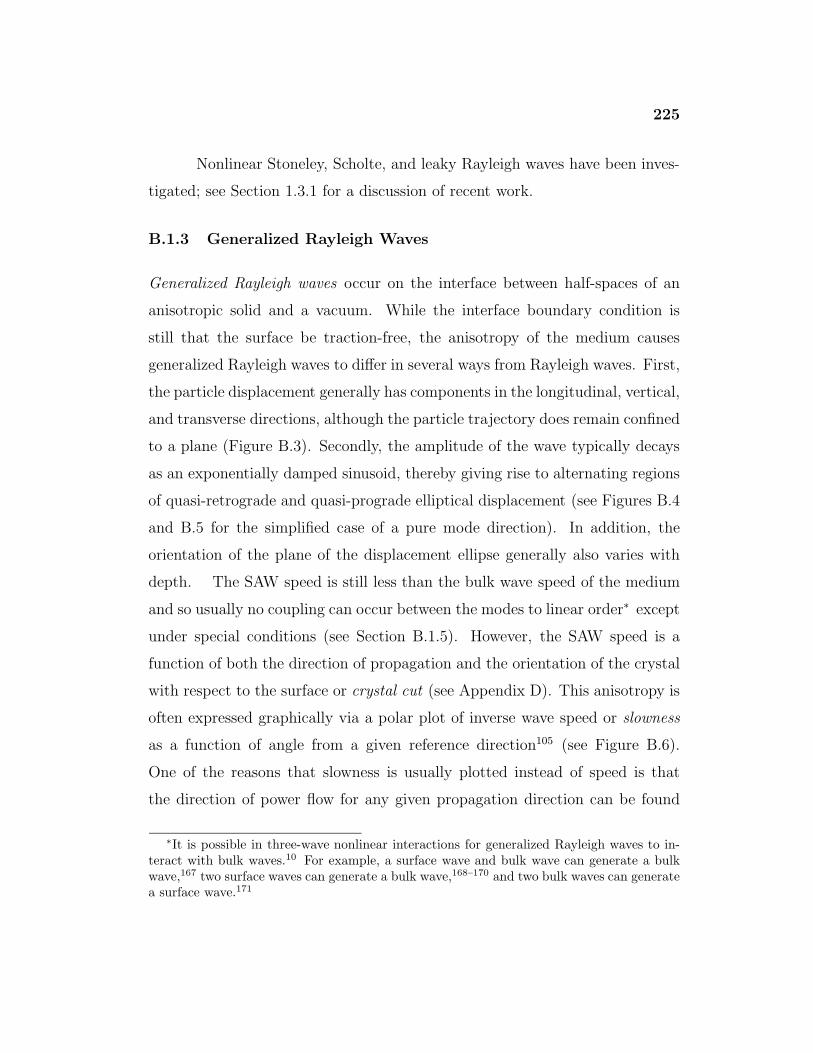
225
Nonlinear Stoneley, Scholte, and leaky Rayleigh waves have been inves-
tigated; see Section 1.3.1 for a discussion of recent work.
B.1.3 Generalized Rayleigh Waves
Generalized Rayleigh waves occur on the interface between half-spaces of an
anisotropic solid and a vacuum. While the interface boundary condition is
still that the surface be traction-free, the anisotropy of the medium causes
generalized Rayleigh waves to differ in several ways from Rayleigh waves. First,
the particle displacement generally has components in the longitudinal, vertical,
and transverse directions, although the particle trajectory does remain confined
to a plane (Figure B.3). Secondly, the amplitude of the wave typically decays
as an exponentially damped sinusoid, thereby giving rise to alternating regions
of quasi-retrograde and quasi-prograde elliptical displacement (see Figures B.4
and B.5 for the simplified case of a pure mode direction). In addition, the
orientation of the plane of the displacement ellipse generally also varies with
depth. The SAW speed is still less than the bulk wave speed of the medium
and so usually no coupling can occur between the modes to linear order∗ except
under special conditions (see Section B.1.5). However, the SAW speed is a
function of both the direction of propagation and the orientation of the crystal
with respect to the surface or crystal cut (see Appendix D). This anisotropy is
often expressed graphically via a polar plot of inverse wave speed or slowness
as a function of angle from a given reference direction105 (see Figure B.6).
One of the reasons that slowness is usually plotted instead of speed is that
the direction of power flow for any given propagation direction can be found
∗It is possible in three-wave nonlinear interactions for generalized Rayleigh waves to in-teract with bulk waves.10 For example, a surface wave and bulk wave can generate a bulkwave,167 two surface waves can generate a bulk wave,168–170 and two bulk waves can generatea surface wave.171
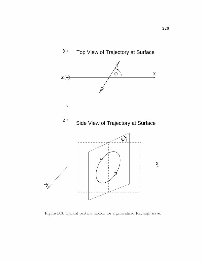
226
φ
-y
z
x
xφz
y Top View of Trajectory at Surface
Side View of Trajectory at Surface
Figure B.3: Typical particle motion for a generalized Rayleigh wave.
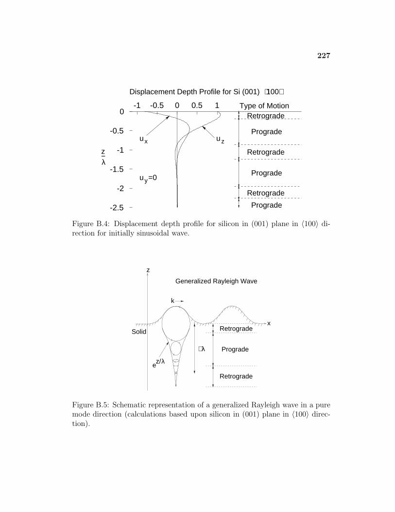
227
-2.5
-2
-1.5
-1
-0.5
0-1 -0.5 0 0.5 1
⟨ ⟩
uz
λz−
uy=0
Retrograde
Prograde
Retrograde
Prograde
Retrograde
Prograde
Type of Motion
ux
100Displacement Depth Profile for Si (001)
Figure B.4: Displacement depth profile for silicon in (001) plane in 〈100〉 di-rection for initially sinusoidal wave.
k
Retrograde
x
z
Generalized Rayleigh Wave
Retrograde
Prograde
Solid
ez/λ
∼λ
Figure B.5: Schematic representation of a generalized Rayleigh wave in a puremode direction (calculations based upon silicon in (001) plane in 〈100〉 direc-tion).
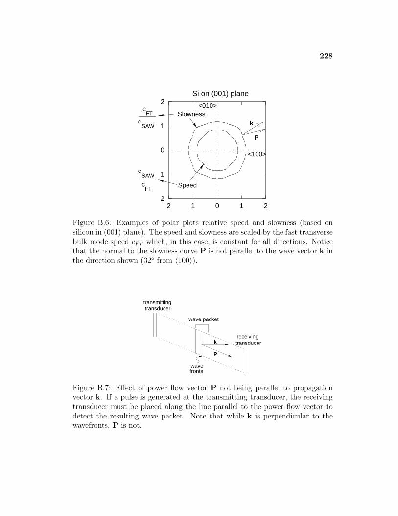
228
2
1
0
1
2
2 1 0 1 2
cSAW
cFT Slowness
Speed
k
P
<100>
<010>
cFT
cSAW
Si on (001) plane
Figure B.6: Examples of polar plots relative speed and slowness (based onsilicon in (001) plane). The speed and slowness are scaled by the fast transversebulk mode speed cFT which, in this case, is constant for all directions. Noticethat the normal to the slowness curve P is not parallel to the wave vector k inthe direction shown (32◦ from 〈100〉).
transducer
P
k
transmitting
transducerreceiving
wave packet
wavefronts
Figure B.7: Effect of power flow vector P not being parallel to propagationvector k. If a pulse is generated at the transmitting transducer, the receivingtransducer must be placed along the line parallel to the power flow vector todetect the resulting wave packet. Note that while k is perpendicular to thewavefronts, P is not.
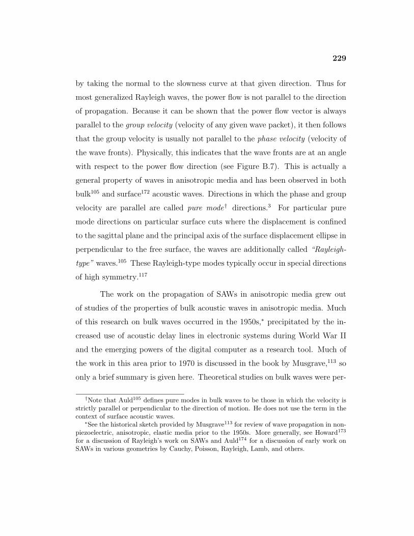
229
by taking the normal to the slowness curve at that given direction. Thus for
most generalized Rayleigh waves, the power flow is not parallel to the direction
of propagation. Because it can be shown that the power flow vector is always
parallel to the group velocity (velocity of any given wave packet), it then follows
that the group velocity is usually not parallel to the phase velocity (velocity of
the wave fronts). Physically, this indicates that the wave fronts are at an angle
with respect to the power flow direction (see Figure B.7). This is actually a
general property of waves in anisotropic media and has been observed in both
bulk105 and surface172 acoustic waves. Directions in which the phase and group
velocity are parallel are called pure mode† directions.3 For particular pure
mode directions on particular surface cuts where the displacement is confined
to the sagittal plane and the principal axis of the surface displacement ellipse in
perpendicular to the free surface, the waves are additionally called “Rayleigh-
type” waves.105 These Rayleigh-type modes typically occur in special directions
of high symmetry.117
The work on the propagation of SAWs in anisotropic media grew out
of studies of the properties of bulk acoustic waves in anisotropic media. Much
of this research on bulk waves occurred in the 1950s,∗ precipitated by the in-
creased use of acoustic delay lines in electronic systems during World War II
and the emerging powers of the digital computer as a research tool. Much of
the work in this area prior to 1970 is discussed in the book by Musgrave,113 so
only a brief summary is given here. Theoretical studies on bulk waves were per-
†Note that Auld105 defines pure modes in bulk waves to be those in which the velocity isstrictly parallel or perpendicular to the direction of motion. He does not use the term in thecontext of surface acoustic waves.
∗See the historical sketch provided by Musgrave113 for review of wave propagation in non-piezoelectric, anisotropic, elastic media prior to the 1950s. More generally, see Howard173
for a discussion of Rayleigh’s work on SAWs and Auld174 for a discussion of early work onSAWs in various geometries by Cauchy, Poisson, Rayleigh, Lamb, and others.
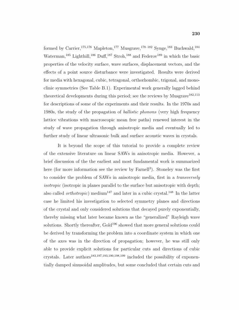
230
formed by Carrier,175,176 Mapleton,177 Musgrave,178–182 Synge,183 Buchwald,184
Waterman,185 Lighthill,186 Duff,187 Stroh,188 and Federov189 in which the basic
properties of the velocity surface, wave surfaces, displacement vectors, and the
effects of a point source disturbance were investigated. Results were derived
for media with hexagonal, cubic, tetragonal, orthorhombic, trigonal, and mono-
clinic symmetries (See Table B.1). Experimental work generally lagged behind
theoretical developments during this period; see the reviews by Musgrave182,113
for descriptions of some of the experiments and their results. In the 1970s and
1980s, the study of the propagation of ballistic phonons (very high frequency
lattice vibrations with macroscopic mean free paths) renewed interest in the
study of wave propagation through anisotropic media and eventually led to
further study of linear ultrasonic bulk and surface acoustic waves in crystals.
It is beyond the scope of this tutorial to provide a complete review
of the extensive literature on linear SAWs in anisotropic media. However, a
brief discussion of the the earliest and most fundamental work is summarized
here (for more information see the review by Farnell3). Stoneley was the first
to consider the problem of SAWs in anisotropic media, first in a transversely
isotropic (isotropic in planes parallel to the surface but anisotropic with depth;
also called orthotropic) medium147 and later in a cubic crystal.148 In the latter
case he limited his investigation to selected symmetry planes and directions
of the crystal and only considered solutions that decayed purely exponentially,
thereby missing what later became known as the “generalized” Rayleigh wave
solutions. Shortly thereafter, Gold196 showed that more general solutions could
be derived by transforming the problem into a coordinate system in which one
of the axes was in the direction of propagation; however, he was still only
able to provide explicit solutions for particular cuts and directions of cubic
crystals. Later authors183,197,193,190,198,199 included the possibility of exponen-
tially damped sinusoidal amplitudes, but some concluded that certain cuts and
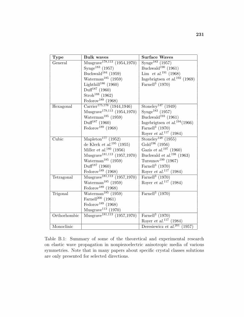
231
Type Bulk waves Surface WavesGeneral Musgrave178,113 (1954,1970) Synge183 (1957)
Synge183 (1957) Buchwald190 (1961)Buchwald184 (1959) Lim et al.191 (1968)Waterman185 (1959) Ingebrigtsen et al.192 (1969)Lighthill186 (1960) Farnell3 (1970)Duff187 (1960)Stroh188 (1962)Fedorov189 (1968)
Hexagonal Carrier175,176 (1944,1946) Stoneley147 (1949)Musgrave179,113 (1954,1970) Synge183 (1957)Waterman185 (1959) Buchwald193 (1961)Duff187 (1960) Ingebrigtsen et al.194(1966)Fedorov189 (1968) Farnell3 (1970)
Royer et al.117 (1984)Cubic Mapleton177 (1952) Stoneley148 (1955)
de Klerk et al.195 (1955) Gold196 (1956)Miller et al.180 (1956) Gazis et al.197 (1960)Musgrave181,113 (1957,1970) Buchwald et al.198 (1963)Waterman185 (1959) Tursunov199 (1967)Duff187 (1960) Farnell3 (1970)Fedorov189 (1968) Royer et al.117 (1984)
Tetragonal Musgrave181,113 (1957,1970) Farnell3 (1970)Waterman185 (1959) Royer et al.117 (1984)Fedorov189 (1968)
Trigonal Waterman185 (1959) Farnell3 (1970)Farnell200 (1961)Fedorov189 (1968)Musgrave113 (1970)
Orthorhombic Musgrave181,113 (1957,1970) Farnell3 (1970)Royer et al.117 (1984)
Monoclinic Deresiewicz et al.201 (1957)
Table B.1: Summary of some of the theoretical and experimental researchon elastic wave propagation in nonpiezoelectric anisotropic media of varioussymmetries. Note that in many papers about specific crystal classes solutionsare only presented for selected directions.
232
directions were “forbidden” from having SAW solutions. Lim and Farnell191
later showed numerically that for a wide variety of crystals that these “forbid-
den” regions were really regions where the surface wave solution degenerated
into a bulk wave solution, now often called an exceptional bulk wave (see Sec-
tion B.1.4). See Table B.1 for a summary of the work done on linear SAWs in
nonpiezoelectric anisotropic media of various symmetries.
In subsequent years, it was proved rigorously that the traction-free sur-
face boundary condition can be satisfied for arbitrary surface cuts and direc-
tions on any anisotropic elastic solid,202,203 although in some cases the only
solution is the exceptional bulk wave. The proofs involved formulating the lin-
earized surface wave problem in formal linear algebraic terms and then deriving
general statements about the possible states of such systems.204 It is interesting
to note that many key developments in the existence and uniqueness problem
came from recognizing the analogies between the the propagation of surface
waves and the propagation of a line dislocation (discontinuity in the elastic
medium) in uniform motion through anisotropic media.188
The nonlinear behavior of SAW in anisotropic media is the subject of
this dissertation. See Section 1.3 for a review of the experimental and theoret-
ical work on this topic.
B.1.4 Quasi-bulk Surface Waves and Exceptional Bulk Waves
In anisotropic media with a free surface, there typically exist three different
bulk waves: one longitudinal or quasi-longitudinal and two shear or quasi-shear
modes.105 In some media, the speed of the the SAW approaches the speed of one
of the shear modes as the propagation direction approaches certain directions
on certain cuts. Typically these are configurations that have a high degree
of symmetry,204 e.g., the [110] direction of the (001) plane of nickel.3 As the
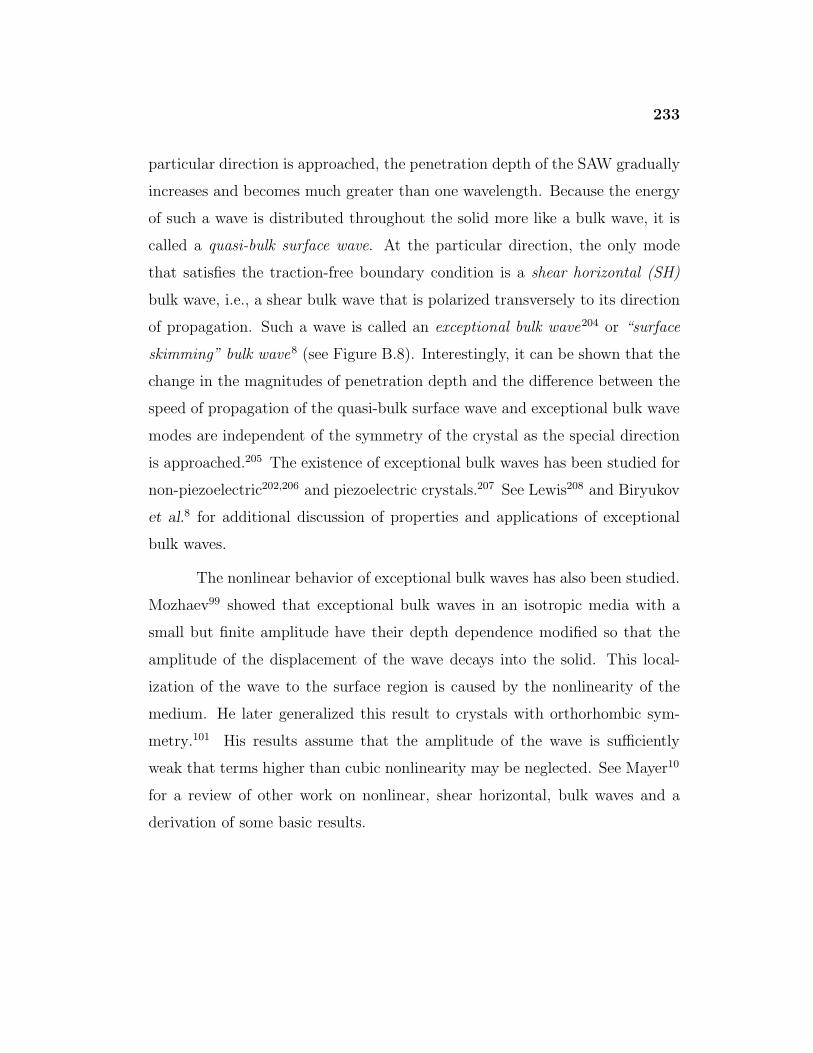
233
particular direction is approached, the penetration depth of the SAW gradually
increases and becomes much greater than one wavelength. Because the energy
of such a wave is distributed throughout the solid more like a bulk wave, it is
called a quasi-bulk surface wave. At the particular direction, the only mode
that satisfies the traction-free boundary condition is a shear horizontal (SH)
bulk wave, i.e., a shear bulk wave that is polarized transversely to its direction
of propagation. Such a wave is called an exceptional bulk wave204 or “surface
skimming” bulk wave8 (see Figure B.8). Interestingly, it can be shown that the
change in the magnitudes of penetration depth and the difference between the
speed of propagation of the quasi-bulk surface wave and exceptional bulk wave
modes are independent of the symmetry of the crystal as the special direction
is approached.205 The existence of exceptional bulk waves has been studied for
non-piezoelectric202,206 and piezoelectric crystals.207 See Lewis208 and Biryukov
et al.8 for additional discussion of properties and applications of exceptional
bulk waves.
The nonlinear behavior of exceptional bulk waves has also been studied.
Mozhaev99 showed that exceptional bulk waves in an isotropic media with a
small but finite amplitude have their depth dependence modified so that the
amplitude of the displacement of the wave decays into the solid. This local-
ization of the wave to the surface region is caused by the nonlinearity of the
medium. He later generalized this result to crystals with orthorhombic sym-
metry.101 His results assume that the amplitude of the wave is sufficiently
weak that terms higher than cubic nonlinearity may be neglected. See Mayer10
for a review of other work on nonlinear, shear horizontal, bulk waves and a
derivation of some basic results.
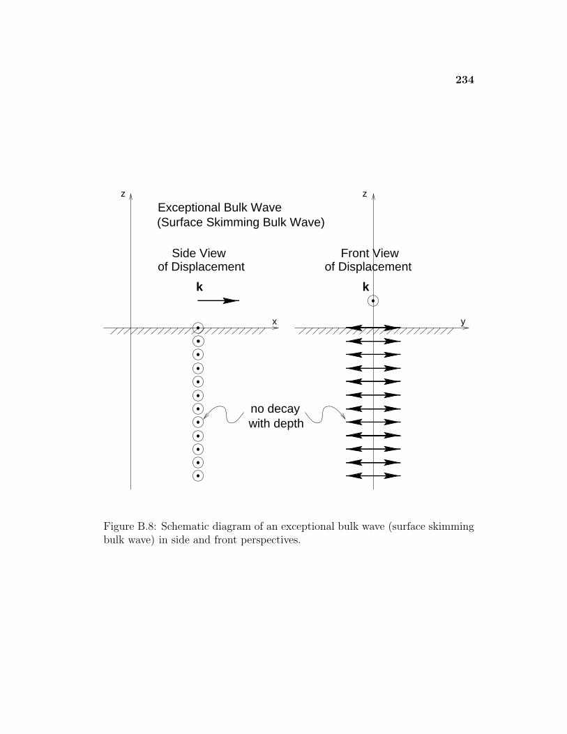
234
no decaywith depth
Exceptional Bulk Wave(Surface Skimming Bulk Wave)
z
x y
kk
z
of DisplacementSide View
of DisplacementFront View
Figure B.8: Schematic diagram of an exceptional bulk wave (surface skimmingbulk wave) in side and front perspectives.
235
B.1.5 Pseudo-surface Waves
Pseudo-surface waves arise in conjunction with the exceptional bulk waves
described above. In the situation that the normal surface wave becomes de-
generate with the normal bulk wave, it is then possible for a new surface wave
solution to exist at a speed higher than the lowest shear wave mode. Away from
the direction associated with the exceptional bulk wave, a pure surface wave
mode is no longer possible, and the pseudo-surface wave mode arises. Close
to the surface, this mode appears like a surface wave in that it decays rapidly
in amplitude away from the surface. However, it differs in that (1) hundreds
or thousands of wavelengths into the solid the wave grows in amplitude and
(2) near the surface its components decay in amplitude as it propagates. This
behavior is consistent with a wave that has its energy flowing or “leaking” at
an angle to the surface into a quasi-shear bulk wave mode. For this reason,
pseudo-surface waves are also called leaky surface waves∗ in some papers.209
This coupling between the surface and bulk modes becomes possible because
the pseudo-surface wave speed is the same as the projection of the speed of
the lowest shear bulk wave traveling at the power flow angle (see Figure B.9).†
Thus the growth of the wave amplitude deep into the solid can be visualized by
observing that energy that reaches a point deep into the solid has come from
areas on the surface where the energy was larger (i.e., larger than the energy
at the surface immediately above that point).3
Pseudo-surface waves have been experimentally observed in several ma-
terials209–213 and predicted to exist in many others.214,3 The experimental ob-
∗Note that pseudo-surface waves differ from leaky Rayleigh waves. In the latter case, theenergy is being radiated into bulk modes of fluid whereas in the former case the energy isbeing radiated into the solid itself.
†In an isotropic medium, bulk wave speeds are the same in all directions. Hence this kindof speed matching cannot occur, and pseudo-surface waves are not possible.
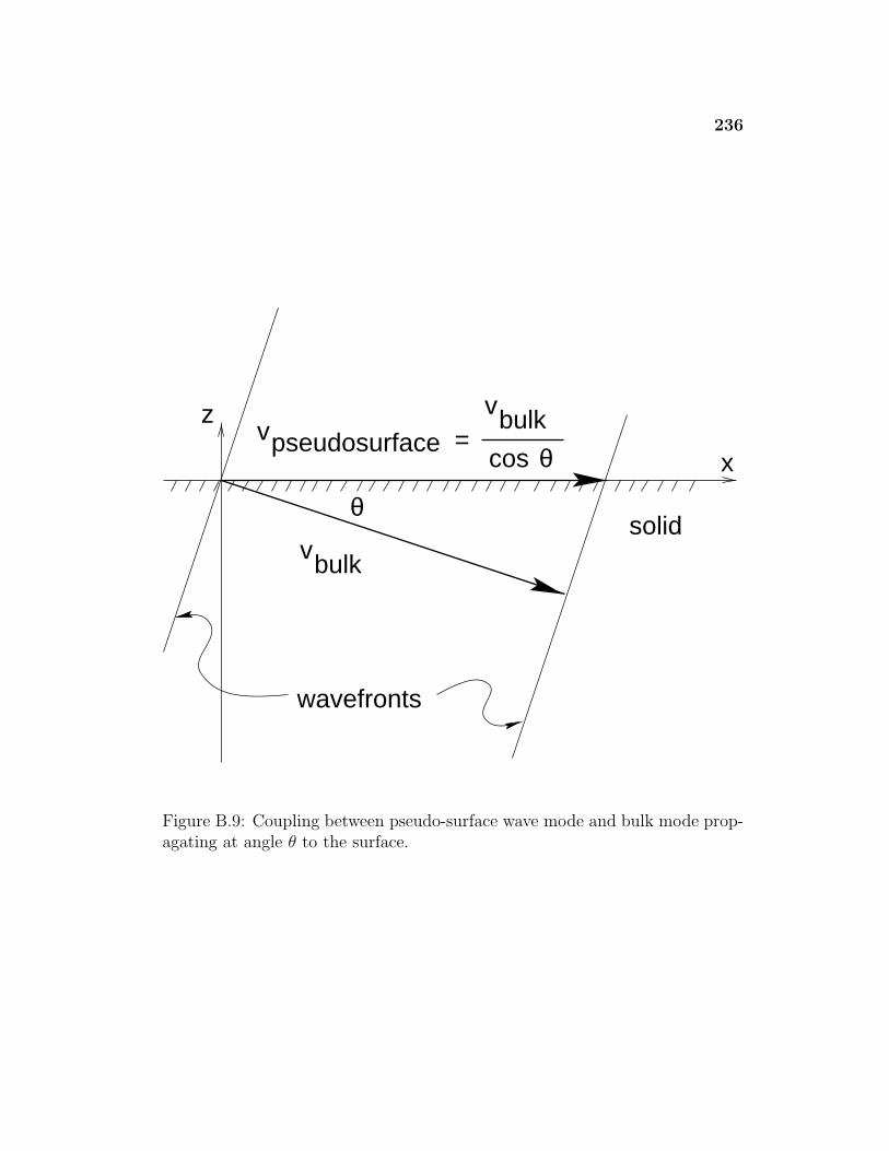
236
pseudosurfacev
vbulk
=cos θ
vbulk
wavefronts
x
solidθ
z
Figure B.9: Coupling between pseudo-surface wave mode and bulk mode prop-agating at angle θ to the surface.
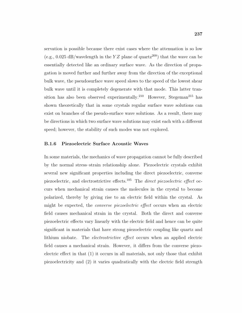
237
servation is possible because there exist cases where the attenuation is so low
(e.g., 0.025 dB/wavelength in the Y Z plane of quartz209) that the wave can be
essentially detected like an ordinary surface wave. As the direction of propa-
gation is moved further and further away from the direction of the exceptional
bulk wave, the pseudosurface wave speed slows to the speed of the lowest shear
bulk wave until it is completely degenerate with that mode. This latter tran-
sition has also been observed experimentally.210 However, Stegeman215 has
shown theoretically that in some crystals regular surface wave solutions can
exist on branches of the pseudo-surface wave solutions. As a result, there may
be directions in which two surface wave solutions may exist each with a different
speed; however, the stability of such modes was not explored.
B.1.6 Piezoelectric Surface Acoustic Waves
In some materials, the mechanics of wave propagation cannot be fully described
by the normal stress–strain relationship alone. Piezoelectric crystals exhibit
several new significant properties including the direct piezoelectric, converse
piezoelectric, and electrostrictive effects.105 The direct piezoelectric effect oc-
curs when mechanical strain causes the molecules in the crystal to become
polarized, thereby by giving rise to an electric field within the crystal. As
might be expected, the converse piezoelectric effect occurs when an electric
field causes mechanical strain in the crystal. Both the direct and converse
piezoelectric effects vary linearly with the electric field and hence can be quite
significant in materials that have strong piezoelectric coupling like quartz and
lithium niobate. The electrostrictive effect occurs when an applied electric
field causes a mechanical strain. However, it differs from the converse piezo-
electric effect in that (1) it occurs in all materials, not only those that exhibit
piezoelectricity and (2) it varies quadratically with the electric field strength
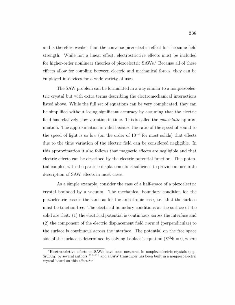
238
and is therefore weaker than the converse piezoelectric effect for the same field
strength. While not a linear effect, electrostrictive effects must be included
for higher-order nonlinear theories of piezoelectric SAWs.∗ Because all of these
effects allow for coupling between electric and mechanical forces, they can be
employed in devices for a wide variety of uses.
The SAW problem can be formulated in a way similar to a nonpiezoelec-
tric crystal but with extra terms describing the electromechanical interactions
listed above. While the full set of equations can be very complicated, they can
be simplified without losing significant accuracy by assuming that the electric
field has relatively slow variation in time. This is called the quasistatic approx-
imation. The approximation is valid because the ratio of the speed of sound to
the speed of light is so low (on the order of 10−5 for most solids) that effects
due to the time variation of the electric field can be considered negligible. In
this approximation it also follows that magnetic effects are negligible and that
electric effects can be described by the electric potential function. This poten-
tial coupled with the particle displacements is sufficient to provide an accurate
description of SAW effects in most cases.
As a simple example, consider the case of a half-space of a piezoelectric
crystal bounded by a vacuum. The mechanical boundary condition for the
piezoelectric case is the same as for the anisotropic case, i.e., that the surface
must be traction-free. The electrical boundary conditions at the surface of the
solid are that: (1) the electrical potential is continuous across the interface and
(2) the component of the electric displacement field normal (perpendicular) to
the surface is continuous across the interface. The potential on the free space
side of the surface is determined by solving Laplace’s equation (∇2Φ = 0, where
∗Electrostrictive effects on SAWs have been measured in nonpiezoelectric crystals (e.g.,SrTiO3) by several authors,216–218 and a SAW transducer has been built in a nonpiezoelectriccrystal based on this effect.219
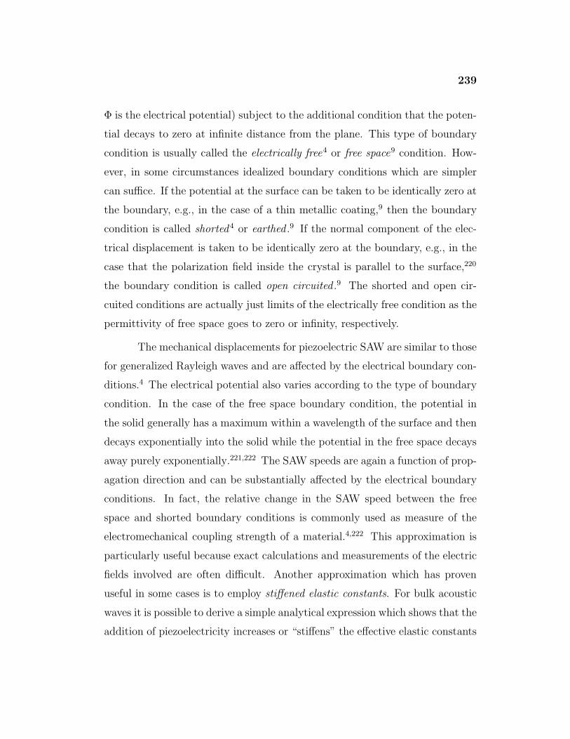
239
Φ is the electrical potential) subject to the additional condition that the poten-
tial decays to zero at infinite distance from the plane. This type of boundary
condition is usually called the electrically free4 or free space9 condition. How-
ever, in some circumstances idealized boundary conditions which are simpler
can suffice. If the potential at the surface can be taken to be identically zero at
the boundary, e.g., in the case of a thin metallic coating,9 then the boundary
condition is called shorted4 or earthed .9 If the normal component of the elec-
trical displacement is taken to be identically zero at the boundary, e.g., in the
case that the polarization field inside the crystal is parallel to the surface,220
the boundary condition is called open circuited .9 The shorted and open cir-
cuited conditions are actually just limits of the electrically free condition as the
permittivity of free space goes to zero or infinity, respectively.
The mechanical displacements for piezoelectric SAW are similar to those
for generalized Rayleigh waves and are affected by the electrical boundary con-
ditions.4 The electrical potential also varies according to the type of boundary
condition. In the case of the free space boundary condition, the potential in
the solid generally has a maximum within a wavelength of the surface and then
decays exponentially into the solid while the potential in the free space decays
away purely exponentially.221,222 The SAW speeds are again a function of prop-
agation direction and can be substantially affected by the electrical boundary
conditions. In fact, the relative change in the SAW speed between the free
space and shorted boundary conditions is commonly used as measure of the
electromechanical coupling strength of a material.4,222 This approximation is
particularly useful because exact calculations and measurements of the electric
fields involved are often difficult. Another approximation which has proven
useful in some cases is to employ stiffened elastic constants. For bulk acoustic
waves it is possible to derive a simple analytical expression which shows that the
addition of piezoelectricity increases or “stiffens” the effective elastic constants
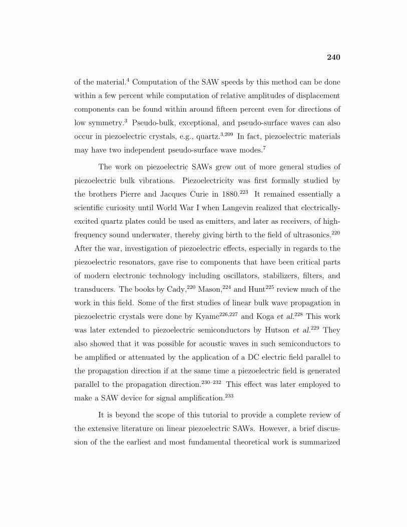
240
of the material.4 Computation of the SAW speeds by this method can be done
within a few percent while computation of relative amplitudes of displacement
components can be found within around fifteen percent even for directions of
low symmetry.3 Pseudo-bulk, exceptional, and pseudo-surface waves can also
occur in piezoelectric crystals, e.g., quartz.3,209 In fact, piezoelectric materials
may have two independent pseudo-surface wave modes.7
The work on piezoelectric SAWs grew out of more general studies of
piezoelectric bulk vibrations. Piezoelectricity was first formally studied by
the brothers Pierre and Jacques Curie in 1880.223 It remained essentially a
scientific curiosity until World War I when Langevin realized that electrically-
excited quartz plates could be used as emitters, and later as receivers, of high-
frequency sound underwater, thereby giving birth to the field of ultrasonics.220
After the war, investigation of piezoelectric effects, especially in regards to the
piezoelectric resonators, gave rise to components that have been critical parts
of modern electronic technology including oscillators, stabilizers, filters, and
transducers. The books by Cady,220 Mason,224 and Hunt225 review much of the
work in this field. Some of the first studies of linear bulk wave propagation in
piezoelectric crystals were done by Kyame226,227 and Koga et al.228 This work
was later extended to piezoelectric semiconductors by Hutson et al.229 They
also showed that it was possible for acoustic waves in such semiconductors to
be amplified or attenuated by the application of a DC electric field parallel to
the propagation direction if at the same time a piezoelectric field is generated
parallel to the propagation direction.230–232 This effect was later employed to
make a SAW device for signal amplification.233
It is beyond the scope of this tutorial to provide a complete review of
the extensive literature on linear piezoelectric SAWs. However, a brief discus-
sion of the the earliest and most fundamental theoretical work is summarized
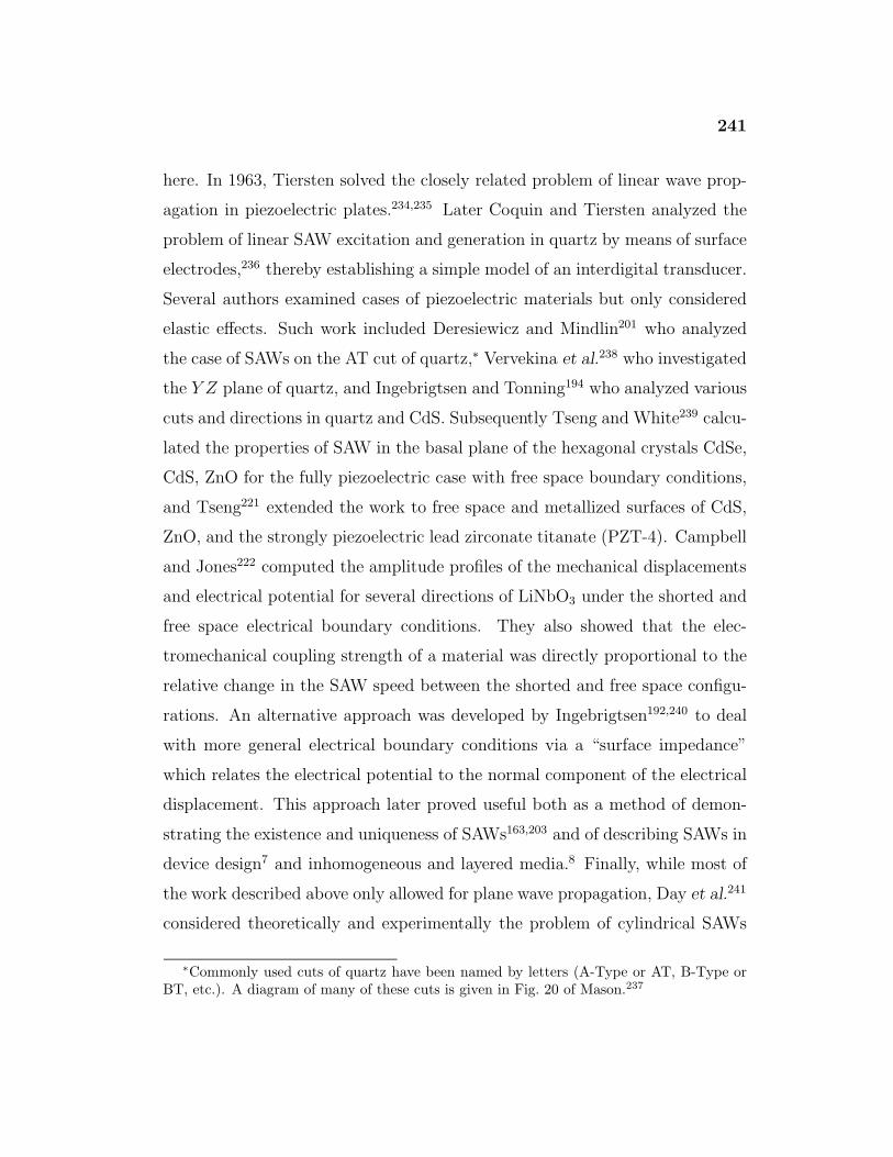
241
here. In 1963, Tiersten solved the closely related problem of linear wave prop-
agation in piezoelectric plates.234,235 Later Coquin and Tiersten analyzed the
problem of linear SAW excitation and generation in quartz by means of surface
electrodes,236 thereby establishing a simple model of an interdigital transducer.
Several authors examined cases of piezoelectric materials but only considered
elastic effects. Such work included Deresiewicz and Mindlin201 who analyzed
the case of SAWs on the AT cut of quartz,∗ Vervekina et al.238 who investigated
the Y Z plane of quartz, and Ingebrigtsen and Tonning194 who analyzed various
cuts and directions in quartz and CdS. Subsequently Tseng and White239 calcu-
lated the properties of SAW in the basal plane of the hexagonal crystals CdSe,
CdS, ZnO for the fully piezoelectric case with free space boundary conditions,
and Tseng221 extended the work to free space and metallized surfaces of CdS,
ZnO, and the strongly piezoelectric lead zirconate titanate (PZT-4). Campbell
and Jones222 computed the amplitude profiles of the mechanical displacements
and electrical potential for several directions of LiNbO3 under the shorted and
free space electrical boundary conditions. They also showed that the elec-
tromechanical coupling strength of a material was directly proportional to the
relative change in the SAW speed between the shorted and free space configu-
rations. An alternative approach was developed by Ingebrigtsen192,240 to deal
with more general electrical boundary conditions via a “surface impedance”
which relates the electrical potential to the normal component of the electrical
displacement. This approach later proved useful both as a method of demon-
strating the existence and uniqueness of SAWs163,203 and of describing SAWs in
device design7 and inhomogeneous and layered media.8 Finally, while most of
the work described above only allowed for plane wave propagation, Day et al.241
considered theoretically and experimentally the problem of cylindrical SAWs
∗Commonly used cuts of quartz have been named by letters (A-Type or AT, B-Type orBT, etc.). A diagram of many of these cuts is given in Fig. 20 of Mason.237
242
in PZT-5. See Table B.2 for a summary of the work done on linear SAWs in
piezoelectric anisotropic media of various symmetries.
The existence of piezoelectric SAWs has also been studied. The prob-
lem becomes more complicated than the nonpiezoelectric case not only by the
addition of the electrical aspect but also because the various mechanical and
electrical boundary conditions have to be taken into account. Lothe and Bar-
nett249 showed that for the case of a mechanically free surface (1) at most one
solution is possible for the electrically open circuited condition and (2) at most
two solutions are possible for the electrically short circuited condition. If two
solutions exist, one must be a Bleustein–Gulyaev wave (see Section B.1.7). No
solutions exist for mechanically clamped surfaces. Alshits et al.250 extended
these results to include piezomagnetic (see Section B.1.8) and piezoelectric–
piezomagnetic materials and provide a table describing the solutions under
all the possible combinations of mechanical, electrical, and magnetic surface
boundary conditions.
B.1.7 Bleustein–Gulyaev Waves
A different kind of SAW occurs in piezoelectric crystals when the sagittal plane
is perpendicular to an axis of twofold rotation. Due to the symmetry of this
situation, the longitudinal and vertical displacements decouple from the trans-
verse displacement and electric potential. The longitudinal and vertical com-
ponents remain intercoupled but propagate as if the piezoelectric constants of
the crystal were set to zero. The transverse displacement and electric potential
also remain intercoupled and give rise to a transversely polarized surface wave
called a Bleustein–Gulyaev wave (BGW)242,243 (See Figure B.10). This type
of wave cannot occur on the surface of a non-piezoelectric solid under normal
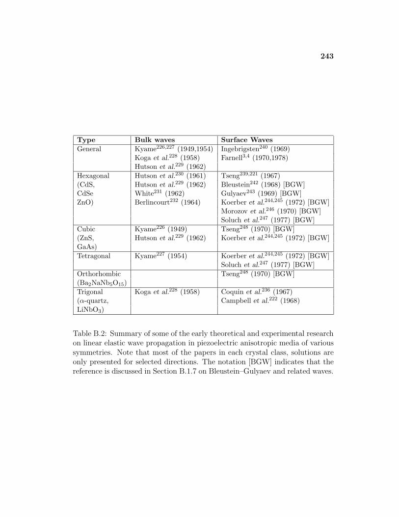
243
Type Bulk waves Surface WavesGeneral Kyame226,227 (1949,1954) Ingebrigsten240 (1969)
Koga et al.228 (1958) Farnell3,4 (1970,1978)Hutson et al.229 (1962)
Hexagonal Hutson et al.230 (1961) Tseng239,221 (1967)(CdS, Hutson et al.229 (1962) Bleustein242 (1968) [BGW]CdSe White231 (1962) Gulyaev243 (1969) [BGW]ZnO) Berlincourt232 (1964) Koerber et al.244,245 (1972) [BGW]
Morozov et al.246 (1970) [BGW]Soluch et al.247 (1977) [BGW]
Cubic Kyame226 (1949) Tseng248 (1970) [BGW](ZnS, Hutson et al.229 (1962) Koerber et al.244,245 (1972) [BGW]GaAs)Tetragonal Kyame227 (1954) Koerber et al.244,245 (1972) [BGW]
Soluch et al.247 (1977) [BGW]Orthorhombic Tseng248 (1970) [BGW](Ba2NaNb5O15)Trigonal Koga et al.228 (1958) Coquin et al.236 (1967)(α-quartz, Campbell et al.222 (1968)LiNbO3)
Table B.2: Summary of some of the early theoretical and experimental researchon linear elastic wave propagation in piezoelectric anisotropic media of varioussymmetries. Note that most of the papers in each crystal class, solutions areonly presented for selected directions. The notation [BGW] indicates that thereference is discussed in Section B.1.7 on Bleustein–Gulyaev and related waves.
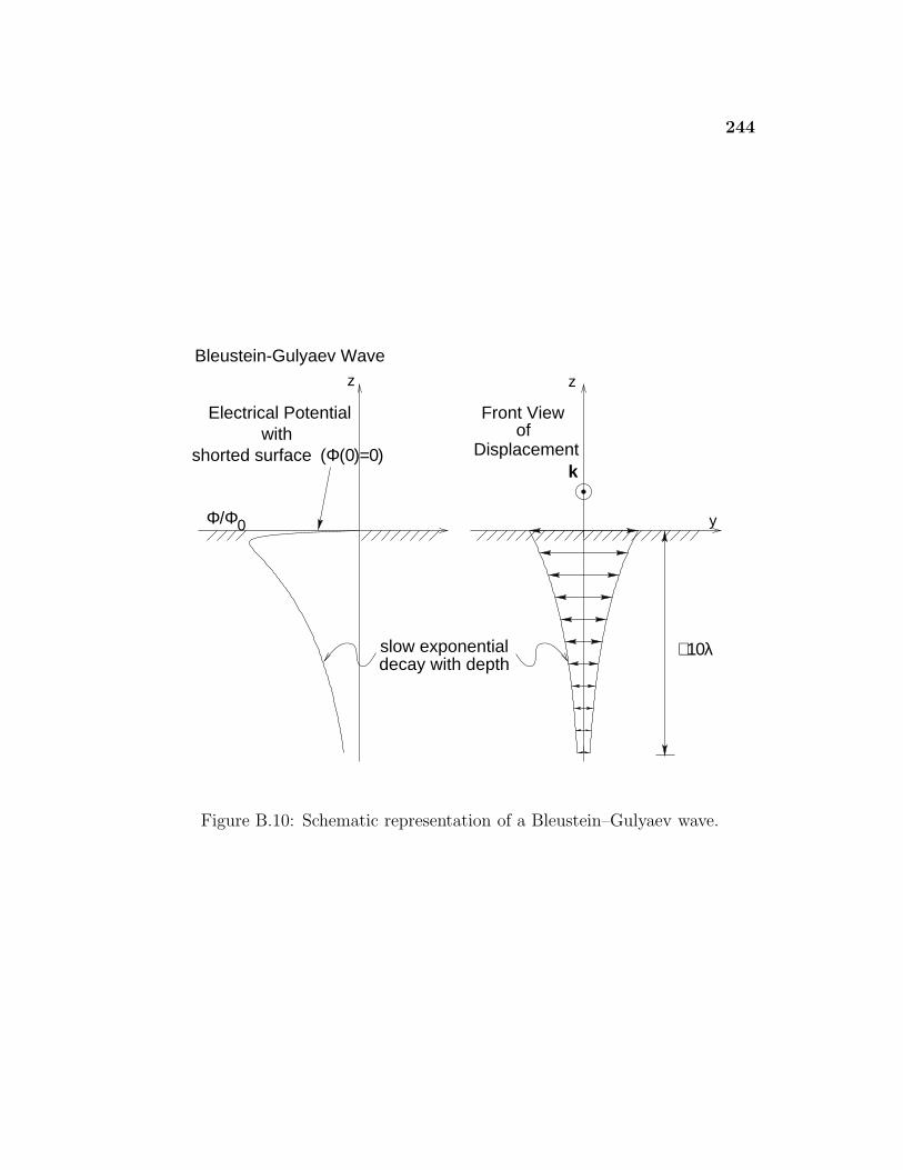
244
decay with depthslow exponential
Φ/Φ0 y
k
∼10λ
z z
shorted surface (Φ(0)=0)
Electrical Potentialwith
Front View
Displacementof
Bleustein-Gulyaev Wave
Figure B.10: Schematic representation of a Bleustein–Gulyaev wave.
245
conditions.∗ As in the case of the piezoelectric SAW considered in the previous
section, the exact form of the BGW depends upon the electrical boundary con-
dition at the surface. However, in both the ‘free space” and shorted boundary
conditions, the amplitude of transverse component decays away purely expo-
nentially from the surface, although the depth of penetration is much greater in
the former than in the latter.4 The potential grows in amplitude until it reaches
an extremum, but then decays away purely exponentially. The depth of pene-
tration in both cases is inversely proportional to the strength of the electrome-
chanical coupling.4,8 Because this coupling is relatively weak even for many
piezoelectric materials, the penetration depth of the waves is large (sometimes
several hundred or thousand wavelengths) as compared to Rayleigh or general-
ized Rayleigh waves. This property, combined with the fact that BGWs have a
larger energy flux as compared to Rayleigh waves, makes BGWs more sensitive
to imperfections in surfaces.8 With both boundary conditions, the velocities of
the BGWs are very close to the velocities of the transversely-polarized shear
bulk waves of the material. Hence, in some ways, BGWs can be considered
to be transversely-polarized shear bulk waves† perturbed into surface waves by
the piezoelectric effects of the medium.4,8
The existence of BGWs has been investigated theoretically,207 and it
has been shown that they exist in materials with several different symmetry
classes.244,245,248 Generalizations of BGWs have been found to propagate along
the interface between two piezoelectric solids252 and two dielectric solids placed
in an external electric field.253 Under circumstances where two piezoelectric
solids are separated by a vacuum gap, BGW can couple from one solid to the
∗Gulyaev and Plessky251 have shown that BGWs may be electrostrictively induced inisotropic dielectrics under the influence of a externally applied electric field.
†Note that BGWs are not the quasi-bulk surface waves described in Section B.1.4 becausethose waves have non-transverse components.
246
other solid via the potential in the gap. Such “gap” waves have been studied
both theoretically251,254,255 and experimentally.8 Acoustoelectric effects and the
amplification of BGWs have also been studied.246,247,256 For more information
on the properties and applications of linear BGWs, see Biryukov et al.8
B.1.8 Piezomagnetic Surface Acoustic Waves
Piezomagnetism, the magnetic analogue to piezoelectricity, occurs when the
mechanical forces couple to the magnetic forces in the material and vice-versa.
The analogue to the electrostrictive effect is the magnetostrictive effect which
occurs when an applied magnetization causes a mechanical strain. It also oc-
curs in all materials and varies quadratically with the magnetization. Gulyaev
et al.257 have shown that in a magnetically ordered crystal with a compen-
sated magnetic moment (i.e., an antiferromagnet) purely shear piezomagnetic
SAWs can exist in certain directions.∗ Examples259 of such piezomagnetic ma-
terials include MnF2 and CoF2. By assuming that (1) the magnetic field is
quasistatic, (2) the surface is mechanically free, and (3) the magnetic potential
is continuous across the surface, they derive expressions for the transverse dis-
placement and magnetic potential inside and outside of the crystal. They show
that unlike Bleustein–Gulyaev waves, which exhibit a superposition of rapidly
and slowly decaying terms in the expression for the electrical potential, the
magnetic potential only has a single term which decays slowly. This property
of deep penetration may make them useful for practical applications.
A limited amount of other work has been performed on piezomagnetic
waves. Parekh260,261 has shown that magnetostrictively induced, purely trans-
∗These piezomagnetic waves should not be confused with the magnetic spin waves ormagnons that can occur on the surface of ferromagnetic materials that are purely magnetic.For more information about magnons, see the review by Mills.258
247
verse shear waves can exist, thereby providing the magnetic analogue to elec-
trostrictively induced Bleustein–Gulyaev waves. Alshits et al.250 has inves-
tigated the conditions for the existence of piezomagnetic SAWs as well as
piezoelectric–piezomagnetic materials and provides a table describing the solu-
tions under all the possible combinations of mechanical, electrical, and magnetic
surface boundary conditions. A few additional references from the Russian lit-
erature on work done on magnetoacoustic waves are also given in this same
paper.
To the knowledge of this author, no work has been performed in the
area of nonlinear piezomagnetic SAWs. However, some work has been done on
linear and nonlinear magnetostrictive SAWs by Abd-Alla and Maugin.262
B.2 Dispersive Waves
Dispersive waves have the property that their wave speed depends upon fre-
quency. Hence a wave packet with many different frequency components may
have each component traveling at a different speed. In the case of strong dis-
persion, wave packets do not form shocks because the harmonic components
of the waves separate relatively quickly compared to the time scale on which
the nonlinear effects occur. Under weaker dispersion, it is possible for effects of
nonlinear distortion to balance the effects of dispersive distortion, thereby giv-
ing rise to waveforms that can propagate without any change in shape. These
waves of permanent form are also called solitons. In contrast with nondispersive
waves, systems that give rise to dispersive waves must define a characteristic
length scale over which the dispersion occurs. For SAWs, this scale is typically
given by a layer depth in layered materials or ridge spacing for corrugated sur-
faces. Because this dissertation focuses exclusively on nondispersive waves, the
brief discussion given below is included only to describe the basic types and
248
properties of dispersive SAWs. Lamb, shear horizontal (SH), Love, perturbed
Rayleigh, Sezawa, and other waves are described below.
Introductions to SAWs with dispersion are given in works by Auld,105
Farnell,4 Lewis,208 and Biryukov et al.8 The books by Ewing, Jardetzky, and
Press263 and Brekhovskikh156 cover some of the earliest work on layered media.
An excellent review on linear surface wave propagation in thin layers is given
by Farnell and Adler.5 Parker9 and Mayer10 review work on nonlinear SAWs
with dispersion. However, the topic of nonlinear SAWs with dispersion is still
very much a topic of current research. For example, Neubrand and Hess264 have
experimentally extracted information about surface layers using laser-excited
SAWs. Even more recent work by Gusev et al.265 and Eckl et al.266 has indicated
that nonlinear SAWs of permanent form may exist in layered half-spaces under
certain conditions.
B.2.1 Plate Waves (Lamb and SH Waves)
Subsequent to his famous paper on surface waves in a semi-infinite half-space,
Rayleigh267 solved the problem of linear waves propagating in a freely vibrating,
infinite, isotropic elastic plate of arbitrary thickness.∗ Around the same time,
Lamb268 also published a paper on the same topic. Because the thickness of the
plate introduces a characteristic length scale, plate waves are dispersive. For
any given wave number, plate waves may only propagate at a set of discrete
frequencies. Such discrete modes can be further classified into even and odd
modes that are symmetric (extension without bending of the middle plane) and
antisymmetric (bending without extension of the middle plane), respectively,
about the centerline of the plate.
∗Auld174 notes that Rayleigh was aware that Cauchy and Poisson had already addressedthe wave propagation problem for thin plates. Moreover, Auld notes that Cauchy had evenconsidered anisotropic plates.
249
Plate waves in isotropic media divide into two independent classes, now
commonly called Lamb waves and shear horizontal (SH) plate waves. Lamb
waves are similar to Rayleigh waves in that they have displacement components
in the longitudinal and vertical directions only (where the vertical direction is
perpendicular to the plate and the longitudinal direction is the direction of
wave propagation). As might be expected from their name, SH waves only
have their displacement in the plate transverse to the direction of propagation.
Physically, the propagation of SH waves can be understood by drawing an
analogy to the propagation of acoustic or electromagnetic waves traveling in
a waveguide, i.e., as plane waves bouncing back and forth off the sides of the
plate at such an angle that the boundary conditions are satisfied. The frequency
cut-off and dispersion exhibited in those systems also occurs with the SH wave
modes. A similar interpretation may be made for Lamb waves but is much
more complicated because mode conversion occurs between the vertical and
longitudinal components at each bounce.
Much additional work has been done on plate waves to extend descrip-
tions to other situations, e.g., curved plates14 and nonpiezoelectric183 and piezo-
electric235 anisotropic plates. See the general references on dispersive SAWs
listed above for additional information and references.
B.2.2 Layer Waves (Love, Perturbed Rayleigh, Sezawa Waves)
A configuration which occurs in many practical situations is a layer of one
solid on the substrate of a different solid with an “empty” half-space above the
layer. Examples include layers that exist in the earth’s crust and layers used to
construct microelectronic components. The thickness of the layer introduces a
characteristic length scale and makes the wave propagation dispersive. In some
ways, the half-space problem and the plate problem can be considered limits
250
of the layered half-space problem as the layer thickness goes to zero and the
substrate’s density or elastic constants go to zero, respectively. As a result,
the waves that can occur in various circumstances are similar in many ways to
those already described. Love waves, perturbed Rayleigh waves, and Sezawa
waves in isotropic materials are briefly described below.
Love waves269 are shear horizontal (transverse displacement only) waves
that occur in the layer and substrate. The displacement typically oscillates
with depth into the layer and then decays into the substrate with the number
of oscillations determining the mode number. They may occur only if the shear
velocity of the layer is less than the shear velocity of the substrate. Suppose
the thickness of the layer is L and the wavelength is λ. When λ/L � 1, the
layer is effectively only a small perturbation to the wave, and the Love wave
speed approaches the substrate shear wave speed. When λ/L � 1, most of the
wave displacement occurs in the layer, and the Love wave speed approaches
the layer shear wave speed. The Love wave speed changes continuously from
one extreme to the other and is, therefore, dispersive.
In contrast, perturbed Rayleigh waves and Sezawa waves are similar to
Rayleigh waves in a half-space in that they have displacement components in
the longitudinal and vertical directions only. They may occur regardless of
whether the layer wave speeds are faster or slower than those of the substrate.
If λ/L � 1, the layer is effectively only a small perturbation to the wave,
and the mode speed approaches the substrate Rayleigh wave speed. When
λ/L � 1, most of the wave displacement occurs in the layer, and the mode
speed approaches the layer Rayleigh wave speed. However, if the Rayleigh wave
speed of the layer is less than the Rayleigh wave speed of the substrate, higher
order modes can occur in which the displacement of the wave oscillates with
depth in the layer and then decays into the substrate. Such higher order modes
251
divide into two classes which correspond to symmetric and antisymmetric Lamb
wave modes in the limit that the density or elastic constants of the substrate
go to zero. The lowest order symmetric mode is called a perturbed Rayleigh
wave, while the lowest order antisymmetric mode is called a Sezawa wave.
Under certain circumstances (typically when the shear wave speeds of the layer
and substrate are similar), the behavior of the Sezawa wave can approach the
behavior of a Stoneley wave near the layer–substrate interface.
Much additional work has been done on surface waves in layered media
to extend descriptions to other situations, e.g., curved surfaces263 and nonpi-
ezoelectric5 and piezoelectric5 anisotropic media. For anisotropic media, the
solutions generally are much more complex because they cannot be decoupled
into Love waves and perturbed Rayleigh and Sezawa waves.270,4 See the gen-
eral references on dispersive SAWs listed above for additional information and
references.
B.2.3 Other Dispersive Surface Waves
Dispersion can arise in other situations than those described in the previous
sections. Composite materials with periodically layered media can have very
complicated mode structures.271,272 Surfaces with periodic corrugations or ran-
dom roughness can introduce a length scale which can cause dispersion; such
corrugations are important for the modeling of SAW devices. See the reviews
of the work in this area by Maradudin,273 Gulyaev and Plessky,274 Biryukov et
al.,8 and Mayer10 for additional information and references.
B.3 Summary
Many different kinds of surface acoustic waves can arise in elastic media due
to interfaces of various kinds. As shown in Table B.3, the waves divide into
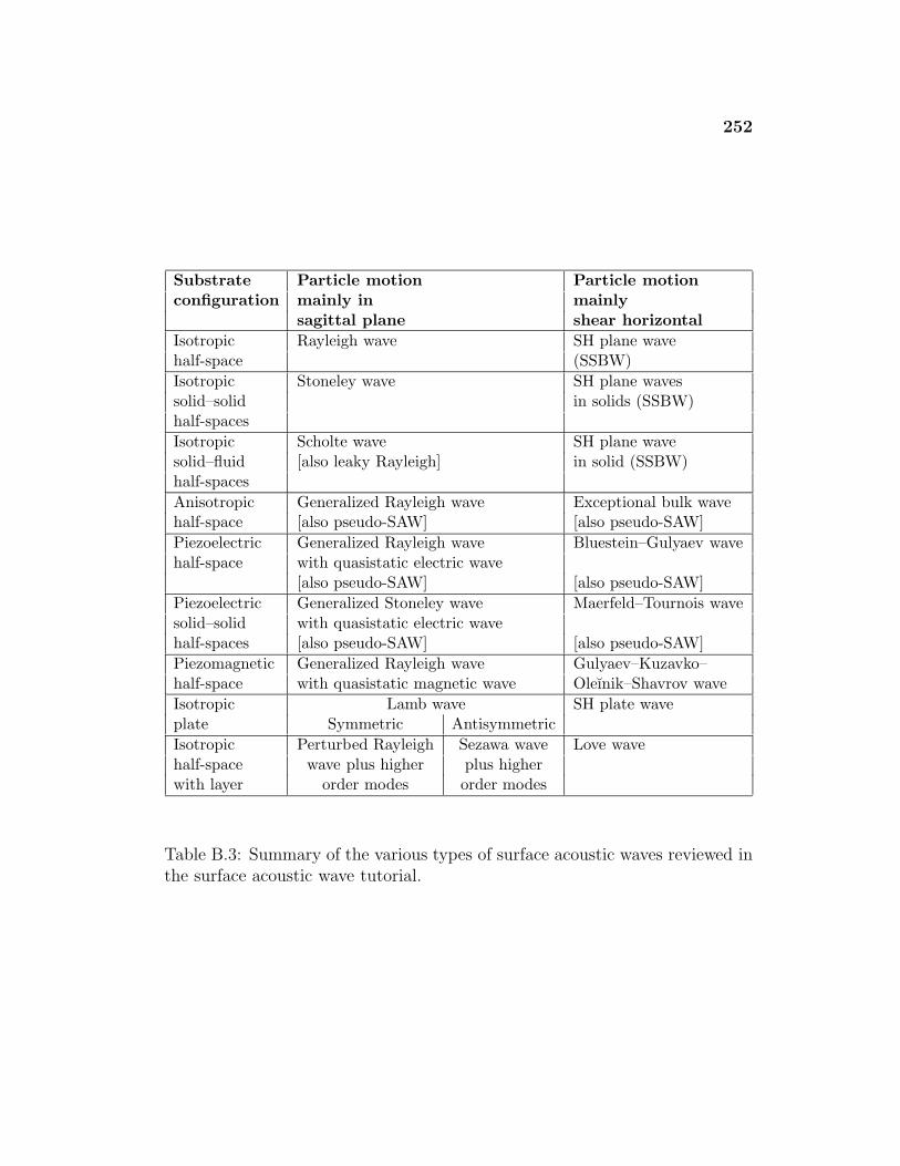
252
Substrate Particle motion Particle motionconfiguration mainly in mainly
sagittal plane shear horizontalIsotropic Rayleigh wave SH plane wavehalf-space (SSBW)Isotropic Stoneley wave SH plane wavessolid–solid in solids (SSBW)half-spacesIsotropic Scholte wave SH plane wavesolid–fluid [also leaky Rayleigh] in solid (SSBW)half-spacesAnisotropic Generalized Rayleigh wave Exceptional bulk wavehalf-space [also pseudo-SAW] [also pseudo-SAW]Piezoelectric Generalized Rayleigh wave Bluestein–Gulyaev wavehalf-space with quasistatic electric wave
[also pseudo-SAW] [also pseudo-SAW]Piezoelectric Generalized Stoneley wave Maerfeld–Tournois wavesolid–solid with quasistatic electric wavehalf-spaces [also pseudo-SAW] [also pseudo-SAW]Piezomagnetic Generalized Rayleigh wave Gulyaev–Kuzavko–half-space with quasistatic magnetic wave Oleınik–Shavrov waveIsotropic Lamb wave SH plate waveplate Symmetric AntisymmetricIsotropic Perturbed Rayleigh Sezawa wave Love wavehalf-space wave plus higher plus higherwith layer order modes order modes
Table B.3: Summary of the various types of surface acoustic waves reviewed inthe surface acoustic wave tutorial.
253
two main categories: those that have particle motion primarily in the sagittal
plane and those that have particle motion that is primarily shear horizontal∗
This tutorial has attempted to clearly describe the basic types and properties
of surface waves which the reader may find mentioned throughout the vast
literature on the subject of surface waves.
∗Maugin275 has specifically reviewed the topic of shear horizontal SAWs and discusses ina unified way many of the waves listed in the table.
Appendix C
Surface Acoustic Wave Applications Tutorial
This tutorial provides an overview of some the basic concepts used to develop
applications for surface acoustic waves (SAWs). It is by no means a complete
review of the field. For more technical and detailed information, see references
listed at the end of each section.
C.1 Signal Processing
Probably the most well-known application of SAWs is a class of solid-state
electronic components generally called SAW devices. These devices process
electrical signals by transforming an electrical input to an electrical output
via the transmission of a SAW across the surface of a piezoelectric crystal.
Electromechanical conversion at both the input and output is usually done via
the use of the interdigital transducer (IDT).276 As Gerard277 describes,
[IDTs] generally consist of interleaved combs of metal electrodes,
with each set extending from a common contact pad. The ID
transducers are photodeposited on the highly polished surface of
a precisely oriented piezoelectric crystal. Upon application of a
voltage to the contact pads, an electric field distribution having
the same spatial period of the electrodes is established between
the electrodes. By means of piezoelectric coupling, these surface-
concentrated fields produce a corresponding elastic strain distribu-
tion.
254
255
At the output, converse piezoelectric coupling causes the elastic strain of the
crystal to induce an electric signal in the IDT. By designing and combining
these IDTs in particular ways, it is possible to construct a wide range of useful
devices including filters, oscillators, pulse compressors and expanders (FM chirp
filters) using linear effects and convolvers, correlators, amplifiers, and memory
elements using nonlinear effects.11 These components have found uses in many
applications, especially mobile and wireless communication devices for personal
communication services (e.g., pagers, cellular phones), wide area networks, and
wireless local area networks.12
A few simple examples are given here to provide a basic understanding
of how such signal processing is accomplished.
In the linear regime, much of the signal processing capability comes from
creative uses of the acoustic transmission across the surface as a delay mech-
anism. Because the speed of sound is so much slower than the speed of light,
the electrical time variation of an input signal can be converted into an acous-
tical spatial variation over a relatively small length. Different points of this
spatial variation can then be sampled and manipulated by IDTs at particular
positions and with particular electrode lengths to process the signal in time.
Consider a SAW device for which an input signal f(t) gives the output signal
f(t) + f(t + τ), where τ is the desired delay time.11 This task is accomplished
by using an IDT to convert the signal f(t) to a SAW of the form f(x−ct) where
c is the SAW speed in the particular direction of propagation. By sampling
the wave with two other IDTs at two points separated by the distance cτ , the
signals f(t) and f(t + τ) are recorded. If these two IDTs are then connected
together the resulting signal is the sum f(t)+ f(t+ τ), as desired. Varying the
lengths of the electrodes varies the amount of electromechanical coupling and
hence the strength of the signal read at any given IDT sampling point.
256
In the nonlinear regime, signal processing is accomplished by exploit-
ing the nonlinearity of the crystalline medium. Consider the case of a SAW
convolver. The two input signals to be convolved are converted to counterprop-
agating SAWs via IDTs on each end of a piezoelectric crystal. A third IDT,
placed between the input IDTs, records the electrical output. If the two input
signals have sufficiently high power levels, then nonlinear harmonic generation
occurs. It can be shown that in such a process the power density of the non-
linearly produced signal is proportional to the product of the power densities
of the generating signals.11 Sampling of the wave by the middle IDT at the
appropriate intervals can then add up the product of the signals (the addition
occuring as described in the previous paragraph) and result in a convolved
signal output.11
Of course, the same effects can be achieved by standard digital electron-
ics. However, the SAW device approach has several advantages over other more
traditional methods. First, the digital electronics equivalent of a SAW device
can often be significantly more complicated.11 Second, traditional approaches
may not work well or at all at very high frequencies, whereas SAW devices
can easily function over a bandwidth from 100 MHz to 2 GHz.11,7 Moreover,
high-performance SAW devices can be cheaply and reliably produced in large
quantities.277,7 Finally, SAW devices can be integrated with other acoustic
and nonacoustic devices. Multiple functions can be implemented on the same
crystal surface and the wave traveling on the surface can be made to inter-
act with other types of external waves (e.g., light, electric, magnetic waves).7
All of these features make SAW devices very attractive for use in solid state,
microelectronic devices. As Ash7 notes,
Every modern television receiver contains at least one SAW filter;
many telecommunications systems—in particular satellite systems—
are dependent on extremely high performance SAW filters; large,
257
and to an increasing extent smaller radar systems use pulse com-
pression SAW filters; one finds high frequency SAW oscillators pen-
etrating electronic systems where previously one was forced to start
with a low frequency quartz crystal source followed by a frequency
multiplier chain. The nonlinear properties of SAW materials form
the basis of signal multiplication, which has opened up a much
wider range of signal processing capabilities. Surface acoustic wave
devices are here to stay.
For more detailed information on SAW devices, see the review by Stegeman
and Nizzoli6 and the books of Oliner13 (editor), Feldmann,7 and Campbell.278,12
C.2 Nondestructive Evaluation
Ultrasonic testing has proven to be a useful tool in the nondestructive evalu-
ation (NDE) of physical systems. By relating acoustic properties to material
or physical properties, it is possible to develop techniques to convert the (of-
ten difficult) task of nondestructively determining physical properties to the
(sometimes easier) task of making acoustic measurements. For example, mea-
surement of the density, transverse sound speed, and longitudinal sound speed
of an isotropic solid allows the Poisson’s ratio, shear modulus, and Young’s
modulus all to be computed.16 Sound velocity measurements have also been
used to determine other quantities including the mixing ratio in composites,
porosity in porcelain, moisture content in plastics, and structure and tensile
strength of gray cast iron.16 As discussed below, measurements of nonlinear
acoustic parameters may provide additional useful information about physical
properties of systems.
While both bulk acoustic waves (BAWs) and SAWs have been used to
perform NDE in wide variety of situations,16,279 the use of SAWs can be more
advantageous than BAWs in certain circumstances. Because SAWs have their
258
energy localized near the surface or interface (within approximately one to
two wavelengths), they are particularly well suited to probe the properties of
surfaces or interfaces. In fact, for thin walled or layered structures, SAWs may
be the only way to probe the sample because BAW testing requires that all
dimensions of the sample to be much larger than a wavelength.14 In addition,
because SAWs only spread two dimensionally and have a relatively smaller
cross-section than BAWs, the amplitudes produced for a given power input
may often be larger for the BAW. This can be important in NDE because often
the detected signals are very small, and the size of the initial amplitude may
decide whether a measurement may be possible at all.
SAWs have been used to characterize a variety of physical properties.
The following sections describe primarily work in the linear regime, but studies
using nonlinear SAWs have been performed as well. The brief descriptions
provided below are by no means a complete review of the extensive work that
has been done in this area; see the references cited in each section for more
information.
C.2.1 Defects
SAWs have been used to detect cracks, pits, voids, segregates, and impuri-
ties.14,280,15 A variety of methods have been developed, but two of the most
common are the pulse–echo and shadow methods. In the pulse–echo method,
defects are detected by measuring the echo reflected from them, and typically
the SAW source also acts as the detector. In the shadow method, separate SAW
source and detectors are used, and the acoustical shadow of the source signal is
measured by the detector. SAWs can exhibit strong reflection and absorption
from surface defects because their surface localization means that nearly the
entire wave is affected. They can also measure small defects quite accurately
259
over a large distance, e.g., a 0.025 mm defect has been detected at a distance
of 4 m using a pulse-echo technique.14 In sheets and tubes, Lamb waves (see
Section B.2.1) may be used with similar results, e.g., inclusions of 1 mm2 or
more in a 4 mm steel plate were reliably detected at radius of 1 m from the
source.14 In addition, Lamb waves can be used to detect segregation of surface
layers of relatively constant thickness because excitation of the surface causes
Lamb modes to occur where they would otherwise not.14 However, SAW meth-
ods have the disadvantages that (1) the presence of foreign materials in the
defects may mask their existence by allowing the SAWs to propagate through
with little change, (2) a rough surface may cause enough scattering that de-
tection of defects may be impossible, (3) visual inspection or liquid penetrant
methods may often be used more easily for many defects.16 In addition, the
interaction of even linear SAWs with very small defects (the size of the mean
free path of air molecules or about 0.1 µm) can be complicated by the nonlin-
ear relation between the compressibility and density of the air in these confined
regions.281 For more detailed information on defect detection with SAW, see
descriptions by Viktorov14 of some of the earliest work and Curtis,15 Doyle and
Scala,282 Stegeman and Nizzoli,6 Kino,280 Krautkramer and Krautkramer,16
and Schmerr283 for more recent efforts.
C.2.2 Plate and Layer Properties
Plates and layers arise in a wide variety of industrial applications. Plates
are common in applications that require metallic sheets or tubes including
ship hulls, airplane bodies, turbine blades, automotive chassis, combustor cas-
ings, and nuclear reactor pressure vessels. Layered systems are important to
many modern applications including very large scale integrated (VLSI) circuits,
micro-electro-mechanical systems (MEMS), reflective coatings on optical com-
ponents, chrome plating for corrosion protection, enamel glazing, low-friction
260
coatings, magnetic thin films for data storage, and hardening surface treatments
in steels. However, the mechanical characteristics of plates and layers, espe-
cially thin films, are not necessarily the same as those measured in the bulk
because the magnitude and directional distribution of mechanical, electrical,
magnetic, and chemical forces change as surfaces or interfaces are approached.
For example, thin films formed by vapor deposition have different properties
than layers formed by other means. Because of their localization in space near
surfaces and interfaces, SAWs have proven useful for determining the proper-
ties of plates and layers. It is well known that SAWs in plates and layers are
dispersive because the plate or layer thickness provides a characteristic length
scale for the system.5 The dispersion causes the SAW speed to vary with fre-
quency and certain modes of propagation to exist only in certain frequency
regimes. Because the dispersion relation and mode structure are functions of
the physical parameters of the system, measurements of the former can give
information about the latter.
Two examples are given here. First, plate thickness can be deduced
by exciting the sample with narrow-band Lamb waves (see Section B.2.1) suc-
cessively over a range of frequencies and looking for mode cut-on. With this
approach, plate thickness measurements from 0.015 mm to several millimeters
with precision of 0.0003 mm have been achieved.14 Secondly, measurements
of dispersion and attenuation in thin films have been performed by examining
the spectra of broad-band, laser-generated SAW pulses at various propagation
distances.264 From this data, the thickness, density, and transverse and longi-
tudinal sound speeds of the layer were extracted for a variety of layer–substrate
combinations. For additional examples see Viktorov,14 Curtis,15 Krautkramer
and Krautkramer,16 and Mayer.10
261
C.2.3 Applied and Residual Stresses
The study of stress in materials is important for many applications. Stresses
caused by the application of an external force are called applied stresses while
stresses that remain even with no force applied are designated residual stresses.
The latter are sometimes induced artificially, e.g., glass has its strength in-
creased by several orders of magnitude by the introduction of surface com-
pressional stresses due to thermal quenching or ion exchange.15 Due to the
acoustoelastic effect, the acoustic velocity of a material changes when a mate-
rial is under stress. For example, when an isotropic material is stressed, the
degeneracy of its transverse bulk wave speed velocities is broken so that differ-
ent polarizations have different speeds.16 Surface waves also exhibit this effect
and have been used to measure applied and residual stresses in solids. One ad-
vantage of SAWs for stress measurements is that they penetrate more deeply
than traditional methods like x-ray diffraction (millimeters vs. microns) and
are less strongly affected by surface roughness.280 However, the acoustic ap-
proach requires careful measurements because the changes in sound speed are
often a fraction of a percent even for large loads.15 An additional difficulty in
such velocity measurements is that stress may also cause changes in the grain
structure from the bulk material and these grain structure changes, in turn,
affect the velocity measurements.15 Residual stress measurements are possible
but tend to be more difficult for a variety of reasons.284,280 For more informa-
tion on ultrasonic stress measurements see the reviews by Curtis,15 Crecraft,284
Kino,280 and Mayer.10
C.2.4 Adhesive Bonding
Quantitative measurement and description of the strength of adhesion (bond-
ing between layers) and cohesion (bonding within a layer) is generally a com-
262
plicated and difficult problem. While adhesion and cohesion can vary with
interface chemistry, contamination, applied stresses, and roughness, it is pos-
sible to minimize and control many of these factors so as to make reasonable
studies possible.285 In layers that are relatively defect-free, bonding strength
is often proportional to elastic modulus.286 With microscopic imperfections,
the strength may be more dependent upon the type and quantity of the de-
fects.286 In both cases, acoustic waves may be useful because their velocity and
attenuation may be related to elastic modulus and defect-induced scattering.
Traditional techniques for measuring adhesion like the scratch and peel test,
while relatively simple, are destructive and often hard to reproduce.285
Some efforts have been made to use linear SAWs to investigate adhesion
between solids. Detection of Stoneley waves via an optical method287 was used
to correlate the attenuation of the waves with surface roughness and hence bond
strength.288 Shear modulus variations in the vicinity of adhesive–adherend
interfaces were determined by measuring the velocity of Rayleigh waves as
a function of adhesive thickness.289,290 Despite work in this area, problems
remain due to the complex nature of the problem and the difficulty of extracting
bond information from acoustic measurements. For example, one problem with
acoustic-based measurements of adhesion is that some organic adhesives are
highly absorptive and may mask poor bonding.16 See Curtis,286 Stegeman
and Nizzoli,6 and Krautkramer and Krautkramer16 for more information on
ultrasonic testing of adhesively bonded structures.
C.2.5 Other Material Properties
Many studies attempt to correlate velocity measurements with material prop-
erties, but attenuation measurements may also be useful. SAW attenuation
is affected by many factors including surface roughness, interaction with ther-
263
mal phonons, interactions with electrons in metals and semiconductors, ion
implantation, molecular in-diffusion, dislocations, and impurities. Often the
sensitivity can be quite high, to the extent that “just breathing on the sur-
face directly can completely attenuate a wave in a few tens of wavelengths.6”
Changes in attenuation have also been used to study phase transitions, e.g.,
superconductive thin layers.6
C.2.6 Nonlinear Ultrasonic NDE
Application of nonlinear BAWs and SAWs to NDE is a topic of current re-
search. Nonlinear effects and BAWs have been used to successfully study crack
size,6 the adhesion of composites,291 precipitate hardening in aluminum,292 and
the carbon content of quenched martensitic steels.72 Less work has been done
with SAWs, probably due to the experimental difficulties of exciting waves
that are large enough to exhibit nonlinear effects but do not destroy the sam-
ple. Several examples are given here. First, SAW excitation of a surface with
microcracks has been shown to generate a significant second harmonic signal,
often as early as 10–20% of the total fatigue life of the sample.293 Secondly,
in systems with “weak” dispersion (i.e. the mode coupling between the fun-
damental and higher harmonics is only slightly perturbed), the combination of
dispersion and nonlinearity typically gives rise to oscillations in the intensity
of the higher harmonics294–296 and has been used to investigate surface rough-
ness due to mechanical polishing.294 Lastly, measurements of the nonlinear
distortion in fused quartz have been performed by examining the spectra of
broad-band, laser-generated SAW pulses at various propagation distances.25
By curve-fitting data to theory, the various third-order elastic constants could
be deduced.
264
C.3 Chemical Sensing
SAW sensors have been developed to detect and identify chemicals. Concep-
tually, these SAW chemical sensors consist of two parts: (1) a material that
contains sites for binding the desired atomic, ionic, or molecular species and
(2) a transducer that has its response changed when the chemicals are present
in the binding material. The binding material is typically a thin film that is
deposited on a piezoelectric substrate. The SAWs are excited and detected
by interdigital transducers (see Section C.1) The adsorption and absorption
of the chemical molecules onto and into the film causes the properties of the
film to change (mass, conductivity, viscoelasticity, etc.). These changes cause
the amplitude and phase of the SAWs to be modified between the input and
output signal. Alternatively, only one IDT may be used with reflector(s) to
set up a SAW resonant cavity, typically with a resonant frequency in the range
20–300 MHz.17 In this method, the presence of the chemical species causes a
shift in the resonance frequency of the device.
Consider, for the moment, SAW devices that measure changes in reso-
nance frequency. Because an IDT transducer produces SAWs at a fixed wave-
length λ (determined by its finger spacing), measurement of the resonance
frequency f0 is effectively a measurement of the SAW velocity v0 = λf0. As
Thompson and Stone write,
The key to SAW chemical sensors, then, is understanding which
factors can affect the acoustic propagation velocity and, therefore,
result in changes of phase and resonance frequency. Following the
notation of Ricco,297 et al., these can be expressed as
∆v
v0=
1
v0
[∂v
∂m∆m +
∂v
∂c∆c +
∂v
∂ε∆ε +
∂v
∂σ∆σ +
∂v
∂T∆T +
∂v
∂P∆P + · · ·
]where m is mass, c is stiffness, ε is dielectric constant, σ is surface
conductivity, T is temperature, and P is pressure. It is possible to
265
obtain expressions for ∆v/v0 for a variety of different cases using
a perturbational approach and the appropriate boundary condi-
tions.105
Many of the earliest SAW sensors used the effects of mass loading alone, but
later sensors have taken more of these factors into account. In fact, the depen-
dence of SAW velocity on these properties has been exploited outside of their ef-
fect on chemical sensing to develop sensors specifically designed to measure tem-
perature,298,299 pressure,300 voltage,301,302 acceleration,303 and magnetic field.304
The small size and resulting portability of SAW sensors allows the
“putting of the instrument into the chemistry, not the chemistry into the instru-
ment.17” Applications have included monitoring workplaces for occupational
hazards, detecting chemical warfare agents, analyzing gas fuels, and determin-
ing ion levels in drinking water.17
The basic design of the SAW chemical sensor was introduced by Wohtjen
and Dessy305,306 in 1979. Subsequently sensors that employ other varieties of
SAWs have also been developed including Lamb waves,307 shear horizontal (SH)
waves,308 and Love waves.309 Each type has advantages and disadvantages. For
example, Lamb wave sensors have the advantages over traditional SAW devices
that they use lower frequencies (2–7 MHz as compared to 30–500 MHz), can
be constructed using standard microfabrication techniques, and can be used
for applications in both the gas and liquid phases (the latter occurs because
the speed of the plate waves is typically less than the compressional wave
speed of gases and liquids and hence no “leaky” waves are produced).17 See
the references at the end of this section for further discussion of the different
devices.
This section is by no means a complete review of this very wide-ranging
field. For more information on SAW chemical sensors, see the book by Thomp-
266
son and Stone.17
C.4 Other Applications
Many other applications have been developed using SAWs. While it is not
possible to provide a complete listing, some brief descriptions and references
are provided here. Note that inclusion in this section does not necessarily imply
that these applications are more important. The division simply expresses the
interests of the author.
C.4.1 Seismology
Seismology is the study of the acoustic disturbances generated by the move-
ments of the earth’s crust. The measurement and understanding of the propa-
gation of SAWs in the earth’s crust often play important roles in seismological
signal analysis. Because SAWs spread two dimensionally and because the near-
earth surface often has little effect on their propagation, they can often prop-
agate long distances and still be detected. Studies have shown that the most
powerful vibrations from earthquakes are in the frequency range of 0.5–5 Hz,
and, close to their source, the strongest ground motions are produced by shear
bulk waves and Love waves.310 In particular, the large horizontal motion of Love
waves is often particularly damaging to the foundations of structures.311 By
combining measurements of BAWs and SAWs at multiple locations and knowl-
edge of the wave speeds of the various signals, seismologists may determine an
earthquake’s location. By similar techniques, the location and magnitude of
underground explosions of nuclear weapons may also be monitored.312,313 How-
ever, recent work has shown that certain kinds of rock are highly nonlinear;314
this nonlinearity has been shown to cause a significant transfer of energy to
higher frequencies in seismic signals.
267
C.4.2 Acoustic Microscopy
Focusing ultrasonic beams on surfaces can excite SAWs. These waves interact
with surface features and, at high frequencies, can be used to produce detailed
acoustical images. These techniques have been used to produce images of many
different media from microelectronic circuits to biological tissues. Acoustic
microscopy has also been used to measure the elastic constants of thin films
and elastic properties of stressed materials.315 For more information, see review
articles by Bertoni,316 Chubachi,317 and Kino280 and the book by Briggs315
(editor).
C.4.3 Surface-skimming Bulk Waves (SSBW) Devices
Surface-skimming bulk waves (SSBW) (see Section B.1.4) combine many of the
advantages of SAWs and BAWs. For example, because the SAW velocity is less
than the BAW velocities, the thermal stability of the delay time for SAWs is
worse than that for BAWs in certain cuts of quartz.8 SSBW devices are used
as high frequency delay lines, filters, and resonators. For more information, see
Biryukov8 (Chapter 6) and Mayer.10
C.4.4 Acoustoelectric Applications
SAWs that propagate along the surface of a piezoelectric crystal have an accom-
panying electric field (see Section B.1.6). This makes it possible for acoustic
signals to interact with the electrons in semiconductors. The effects can often
be highly nonlinear due to the nonlinear relation between the current and field
in semiconductors. Applications include amplifiers, correlators, and optical im-
agers. For more information, see the review articles by Kino318 and Stern319
and Biryukov8 (Chapter 2).
268
C.4.5 Acoustooptic Applications
SAWs that propagate across the surface of certain materials modulate the index
of refraction of the material. This makes it possible for acoustic signals to
interact with light. Applications include optical diffraction gratings, deflectors,
modulators, and filters. As an example, modulators are used for switching light
beams in laser printers and laser communications.320 For more information, see
review articles by Chang,321 Schmidt,322 and Stegeman.323
C.4.6 Ultrasonic Motors
An ultrasonic motor is a type of actuator that uses mechanical vibrations in
the ultrasonic range as its drive source.324 For example, suppose two rings are
placed on top of one another so that they touch. Then the excitation of a
traveling Lamb wave in one ring (stator), due to frictional forces, causes the
other ring (rotor) to move in the direction of the traveling wave. Such traveling
wave motors have been developed commercially for use in auto-focusing camera
lenses. Alternatively, the frictional interaction between a small object on a
surface and the movement of a SAW can cause the object to move. As a
result, micromechanical motors can be produced that can rapidly make position
changes of an object with the accuracy of nanometers, e.g., see Kurosawa et
al..325 Ultrasonic motors also have the advantages that they are low-speed
but high-torque, have small size, and operate quietly. In addition, they are
unaffected by the presence of high magnetic fields (unlike traditional electric
motors) and, therefore, may be used in applications like magnetic resonance
imaging machines and magnetic levitating trains. See the books by Sashida and
Kenjo324 and Ueha et al.326 for comprehensive overviews of ultrasonic motor
research.
269
C.4.7 Surface Acceleration
Laser-generated, nonlinear SAWs have been used to produce local surface ac-
celerations that are high enough to throw off weakly adhering microparticles.327
Applications of this technique include cleaning microparticles from the surface
of semiconductor wafers in a vacuum, measurement of the adhesive forces of
microparticles, and visualization of the distribution of surface acoustic wave
pulses. The latter application was realized to image SAW focusing in crys-
tals.328
C.4.8 Touch Screen Technology
SAWs may be used to create screens that are sensitive to a user’s touch. A set
of SAW transducers and reflectors is arranged around the perimeter of a glass
panel. When a finger touches the screen, the SAWs are absorbed at that point
causing a touch event to be detected at that location. This type of screen has
the highest resolution and durability of any type of touch screen technology,
although it can be sensitive to large amounts of dirt, dust, and water. See the
paper by Adler329 for a brief review and discussion of this topic.
C.4.9 Animal Bioacoustics
A variety of animals are known to employ SAWs for short range communication.
Certain species of insects, frogs, kangaroo rats, mole-rats and chameleons are
able to generate and detect low frequency SAWS. For more information, see
the article by Narins.330
270
C.5 Summary
A remarkable variety of applications have been developed for SAWs in both the
linear and nonlinear regimes. With the ongoing research in the generation and
modeling of nonlinear SAWs, it is not unreasonable to expect that additional
applications will be found in future.
Appendix D
Crystals and Miller Index Notation
The properties of surface acoustic waves in anisotropic crystals depend critically
upon how the surface is oriented with respect to the crystal axes and the direc-
tion that the wave is propagating. The surfaces of cut crystals have tradition-
ally been described using a crystallographic convention called Miller indices.
Miller indices are defined by finding three noncollinear atoms on the surface
that intersect the crystal axes and then applying the following method331:
1. Find the intercepts of the three basis axes in terms of the
lattice constants.
2. Take the reciprocals of these numbers and reduce to the small-
est three integers having the same ratio. The result is enclosed
in parentheses (hkl).
Note that if the Miller indices are interpreted as vector components, the re-
sulting vector is normal to the surface of the cut. Directions are specified in a
different way331:
The indices of a direction in a crystal are expressed as the set of the
smallest integers which have the same ratios as the components of
a vector in the desired direction referred to the axis vectors. The
integers are written in square brackets, [uvw]. The x axis is the
[100] direction; the −y axis is the [010] direction. A full set of
equivalent directions is denoted this way: 〈uvw〉.
271
272
Figure D.1 shows some typical crystal cuts and how they are specified
using the Miller index notation. For example, the (001) plane intersects the
crystal axes at, x = ∞ (1/∞ = 0), y = ∞, and z = 1. Similarly, the (111)
plane intersects the crystal axes at x = 1, y = 1, and z = 1.
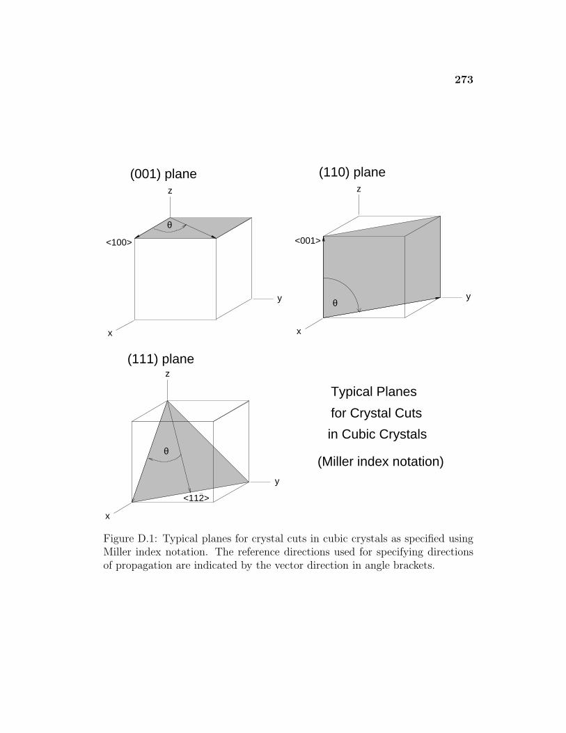
273
Typical Planes
for Crystal Cuts
in Cubic Crystals
(Miller index notation)y
x
z
θ
<112>
(111) plane
θ
y
x
z
<100>
(001) plane
y
x
z
<001>
(110) plane
θ
Figure D.1: Typical planes for crystal cuts in cubic crystals as specified usingMiller index notation. The reference directions used for specifying directionsof propagation are indicated by the vector direction in angle brackets.
Appendix E
Derivation of the Integral Transform Between
Velocity Components of a SAW in a Crystal
As stated in Section 2.3, the velocity components of SAW waveforms in a crystal
can be related by the integral transforms given by Eq. (2.100). In this section,
a derivation of this result is provided.
According to Eq. (2.89), the velocity component on the surface x3 = 0
in the xj direction is given by
vj(x, τ) =
∞∑n=−∞
vn(x)unje−inω0τ =
∞∑n=−∞
vjn(x)e−inω0τ , (E1)
where
unj =
{Bi =
∑3s=1 β
(s)i for n > 0
B∗i =
∑3s=1(β
(s)i )∗ for n < 0
}= |Bi|ei(n/|n|)φBi , (E2)
and the constants β(s)i from linear theory are defined in Section 2.1. Equa-
tion (E1) can be rewritten as
vj(x, τ) =
∞∑n=−∞
[unj
uni
][vn(x)uni]e
−inω0τ . (E3)
Substitution of Eq. (E2) into Eq. (E3) immediately yields
vjn(x) =
{(Bj/Bi)vin(x) for n > 0(B∗
j /B∗i )vin(x) for n < 0
, (E4)
which is the result relating the spectral amplitudes given in Eq. (2.99).
274
275
Calculations relating the time waveforms can be most easily carried out
by considering the problem in terms of Fourier transforms instead of Fourier
series. The continuous analogue to the series of Eq. (E1) is
vj(x, τ) =1
2π
∫ ∞
−∞v(x, ω)uj(ω)e−iωτ dω =
1
2π
∫ ∞
−∞vj(x, ω)e−iωτ dω , (E5)
where
uj(ω) =
{Bj for ω > 0B∗
j for ω < 0
}= |Bi|ei(ω/|ω|)φBi . (E6)
Correspondingly, the continuous analogue of Eq. (E3) is given by
vj(x, τ) =1
2π
∫ ∞
−∞
[uj(ω)
ui(ω)
][v(x, ω)ui(ω)]e−iωt dω . (E7)
Let F (x, ω) = v(x, ω)ui(ω) and
G(ω) =uj(ω)
ui(ω)=
{Bji = Bj/Bi for ω > 0B∗
ji = B∗j /B
∗i for ω < 0
, (E8)
so that
vj(x, τ) =1
2π
∫ ∞
−∞G(ω)F (x, ω)e−iωt dω . (E9)
Here G(ω) and F (x, ω) can be interpreted as Fourier transforms of undeter-
mined functions g(τ) and f(x, τ). Under this interpretation, the Convolution
Theorem111 can be applied to Eq. (E9) to yield
vj(x, τ) = g ∗ f =
∫ ∞
−∞f(x, τ ′)g(τ − τ ′) dτ ′ . (E10)
Hence, the computation of f(x, τ) and g(τ) fully determines the integral trans-
form.
The function f(x, τ) is found by taking the inverse Fourier transform of
F (x, ω) = vi(x, ω). This can be computed immediately from Eq. (E5)
f(x, τ) =1
2π
∫ ∞
−∞F (x, ω)e−iωτ dω =
1
2π
∫ ∞
−∞vi(x, ω)e−iωτ dω = vi(x, τ) .
(E11)
276
The function g(τ) is found by taking the inverse Fourier transform of G(ω):
g(τ) =1
2π
∫ ∞
−∞G(ω)e−iωτ dω . (E12)
However, substitution of Eq. (E8) followed straightforward evaluation of this
integral fails because the integral is not absolutely convergent. Instead, com-
pute the inverse transform
gr(τ) =1
2π
∫ ∞
−∞G(ω)e−r|ω|e−iωτ dω , (E13)
and take the limit
limr→0
gr(τ) = g(τ) . (E14)
Evaluation of the integral of Eq. (E13) is done as follows:
gr(τ) =1
2π
∫ ∞
−∞G(ω)e−r|ω|e−iωτ dω
=1
2π
[∫ 0
−∞B∗
jie(r−iτ)ω dω +
∫ ∞
0
Bjie(−r−iτ)ω dω
]=
1
2π
[B∗
ji
e(r−iτ)ω
r − iτ
∣∣∣∣0−∞
+ Bji
e(−r−iτ)ω
−r − iτ
∣∣∣∣∞0
]
=1
2π
[B∗
ji
r − iτ+
Bji
r + iτ
].
(E15)
In order to properly evaluate the limit as r → 0, Eq. (E15) may be further
rewritten as
gr(τ) =1
2π
[B∗
ji
r − iτ+
Bji
r + iτ
]=
1
2π
[B∗
ji(r + iτ) + Bji(r − iτ)
r2 + τ 2
]=
1
2π
[(Bji + B∗
ji)r − (Bji − B∗ji)iτ
r2 + τ 2
]=
(Bji + B∗
ji
2
)1
π
r
r2 + τ 2+
(Bji − B∗
ji
2i
)1
π
τ
r2 + τ 2
= Re(Bji)1
π
r
r2 + τ 2+ Im(Bji)
1
π
τ
r2 + τ 2.
(E16)
277
It then follows that
g(τ) = limr→0
gr(τ) = Re(Bji) limr→0
1
π
r
r2 + τ 2+ Im(Bji) lim
r→0
1
π
τ
r2 + τ 2. (E17)
Evaluating the first limit on the right side of Eq. (E17) yields
limr→0
1
π
r
r2 + τ 2= lim
r→0
1
π
1/r
1 + (1/r)2τ 2= lim
n→∞1
π
n
1 + n2τ 2= lim
n→∞δn(τ) = δ(τ) ,
(E18)
where δ(τ) is the Dirac delta function defined such that112∫ ∞
−∞f(τ)δ(τ) dτ = f(0) . (E19)
The last equality in Eq. (E18) is a well-known result from distribution theory.112
Evaluating the second limit on the right side of Eq. (E17) yields
limr→0
1
π
1
r2 + τ 2=
1
πτ(E20)
Substituting Eqs. (E18) and (E20) into Eq. (E17) gives
g(τ) = Re(Bji)δ(τ) + Im(Bji)1
πτ. (E21)
Substitution of Eqs. (E11) and (E21) into the convolution of Eq. (E10) then
gives the result
vj(x, τ) =
∫ ∞
−∞f(x, τ ′)g(τ − τ ′) dτ ′
=
∫ ∞
−∞vi(x, τ ′)
[Re(Bji)δ(τ − τ ′) + Im(Bji)
1
π(τ − τ ′)
]dτ ′
= Re(Bji)vi(x, τ) + Im(Bji)1
π
∫ ∞
−∞
vi(x, τ ′)τ − τ ′
dτ ′
= Re(Bji)vi(x, τ)− Im(Bji)1
π
∫ ∞
−∞
vi(x, τ ′)τ ′ − τ
dτ ′ .
(E22)
By definition,111 the Hilbert transform is
H[h(τ)] =1
πPr
∫ ∞
−∞
h(τ ′)τ ′ − τ
dτ ′ . (E23)
278
Substituting Eq. (E23) and Bji = Bj/Bi into Eq. (E22) yields
vj(x, τ) = Re(Bj/Bi)vi(x, τ)− Im(Bj/Bi)H[vi(x, τ)] . (E24)
This is the result listed in Eq. (2.100).
Appendix F
Additional Discussion of Complex-Valued
Nonlinearity Parameters
The basic results of Section 6.2.2 can be derived in an alternate way. This
alternative method provides additional insight into relationship between the
various linear and nonlinear quantities described by the theory presented in
Chapter 2.
Instead of determining the effect of phase changes on the spectral am-
plitudes, here the focus is on phase changes in the linear amplitude factors
β(s)j . As stated in Section 2.1.2, the absolute phase of the β
(s)j terms is not
determined by the theory; only relative phases between the β(s)j are fixed. To
see this, recall from Eq. (2.9) that the particle displacement for a linear SAW
in a crystal can be written in the form
uj =
3∑s=1
β(s)j eik(ls·x−ct) =
3∑s=1
β(s)j eiζskx3ei(kx1−ω0t) , (F1)
where ls = (l(s)1 , l
(s)2 , l
(s)3 ) = (1, 0, ζs), and the β
(s)j = Csα
(s)j are defined by
Eq. (2.11):
ci3kl
3∑s=1
β(s)j l
(s)l = 0 , (F2)
as a result of the stress-free boundary condition in Eq. (2.10). To examine the
effects of changing the absolute phase, let
β(s)θj = β
(s)j eiθ (F3)
279
280
for some phase angle 0 ≤ θ ≤ 2π. Multiplying both sides of Eq. (F2) by eiθ
and substituting Eq. (F3) into the result yields
ci3kl
3∑s=1
β(s)θj l
(s)l = 0 , (F4)
which shows that the β(s)θj are also valid solutions for the linear problem. The
only other condition on the β(s)θj terms is the normalization condition of the
nonlinear theory given in Eq. (2.27)
∫ 0
−∞
∣∣∣∣∣3∑
s=1
β(s)j eiζsz′
∣∣∣∣∣2
= 1 . (F5)
However, because |β(s)θj | = |β(s)
j |, it follows immediately that
∫ 0
−∞
∣∣∣∣∣3∑
s=1
β(s)θj eiζsz′
∣∣∣∣∣2
= 1 . (F6)
Thus, it has been shown if the linear amplitude factors β(s)θj are solutions of the
linear problem and satisfy the normalization condition of the nonlinear theory,
then the amplitude factors β(s)θj defined by Eq. (F3) are also valid solutions.
However, changing the phase of linear amplitude factors, also changes
other quantities in the theory which depend upon them. In particular, the rep-
resentation of the nonlinearity matrix elements, depth dependence functions,
and waveforms are all changed.
First, consider changes in the nonlinearity matrix elements under the
transformation caused by introducing β(s)θj in place of β
(s)j . Eq. (2.26) then
becomes
F θs1s2s3
= Fs1s2s3eiθ . (F7)
281
According to Eq. (2.33) for n = l + m > 0, it then follows that
Sθlm(−n) =
3∑s1,s2,s3=1
F θs1s2s3
lζs1 + mζs2 − nζ∗s3
= Slm(−n)eiθ . (F8)
For n = l + m < 0, the symmetry property of Eq. (6.3) [also Hamilton et al.,33
Eq. (80)] may be used to show that
Sθlm(−n) = (Sθ
(−l)(−m)n)∗ = (S(−l)(−m)neiθ)∗ = S∗(−l)(−m)ne−iθ = Slm(−n)e
−iθ .
(F9)
Combining Eq. (F8) and Eq. (F9) implies that for all n,
Sθlm(−n) = Slm(−n)e
i(n/|n|)θ . (F10)
By multiplying both sides of Eq. (F10) by −1/c44 and using Eq. (4.5), it im-
mediately follows that
Sθlm(−n) = Slm(−n)e
i(n/|n|)θ . (F11)
Equation (F11) matches the notation introduced previously in Eq. (6.4).
Next, consider the effect of transforming the depth functions under the
substitution β(s)θj = |β(s)θ
j | exp(iφ(s)θj ) for β
(s)j = |β(s)
j | exp(iφ(s)j ). By Eq. (F3),
it follows that
|β(s)θj | = |β(s)
j | , (F12a)
φ(s)θj = φ
(s)j + θ . (F12b)
Using Eqs. (F12), the depth functions given in Eq. (2.13) transform as
uθnj(z) =
3∑s=1
|β(s)θj | exp[i(n/|n|)φ(s)θ
j ]
=3∑
s=1
|β(s)j | exp[i(n/|n|)(φ(s)
j + θ)]
= unj(z)ei(n/|n|)θ .
(F13)
282
Note that uθnj = [uθ
(−n)j ]∗, as required by Eq. (2.13).
Finally, if the transformed velocity waveforms are defined as
vθj (x, z, τ) =
∞∑n=−∞
vn(x)uθnj(z)e−inω0τ , (F14)
then Eq. (F14) is the analogue of Eq. (6.9). The only difference between them
is that here Eq. (F14) introduces the phase factor ei(n/|n|)θ, whereas Eq. (6.9)
introduces the phase factor of e−i(n/|n|)θ from the transformed spectral ampli-
tudes of Eq. (6.8):
vn(x) = vn(x)e−i(n/|n|)θ . (F15)
In other words, Figures 6.5 and 6.6 can just as well be derived from Eq. (F14)
by replacing θ with −θ.
The close relationship between Eq. (F14) and Eq. (6.9) is not coinciden-
tal. Because the transformation of the nonlinearity matrix given in Eq. (F11)
above also implies Eq. (F15) (by the derivation in Chapter 6), the waveforms
should, strictly speaking, be reconstructed using both the transformations of
the spectral amplitudes vn(x) and the depth functions unj(z). Define the wave-
form function
vθj (x, z, τ) =
∞∑n=−∞
vθn(x)uθ
nj(z)e−inω0τ . (F16)
Substituting Eqs. (F13) and (F15) into Eq. (F16) immediately implies that for
all θ,
vθj (x, z, τ) = vj(x, z, τ) . (F17)
In other words, the velocity waveforms are invariant under the change in the ab-
solute phase of the β(s)j . This result is expected because the internal mathemat-
ical representation of the absolute phase cannot affect the physical waveforms.
283
The partial waveform transformations [partial in the sense that only vθn(x) or
only uθnj(z) are used] show how breaking the invariance of Eq. (F17) is similar
to introducing anisotropy into the physical system and thereby changing the
phase relationship between the nonlinearity matrix elements, linear amplitude
factors, and spectral components from the isotropic case.
To close, this section provides a detailed derivation of Eqs. (6.19). These
equations give the values of the transformation phase θ that are appropriate use
in conjunction with Figures 6.5 and 6.6 to characterize the various waveforms
of the velocity components. Assume that the phases differences between the
surface linear amplitude components B1, B2, and B3 are known. For example,
consider the vertical velocity component at the surface, and the idealized cases
where all the nonlinearity matrix elements have the phase θ = θlong = arg(Slm).
(If the matrix elements are not all the same phase, use a matrix element rep-
resentative of the average phase of the elements.) Then Eq. (6.10) can be
rewritten as
v3(x, τ) =
∞∑n=−∞
vθn(x)|B3|ei(n/|n|)φB3e−inω0τ
=|B3||B1|
∞∑n=−∞
vθn(x)|B1|ei(n/|n|)φB1ei(n/|n|)(φB3−φB1)e−inω0τ
=|B3||B1|
∞∑n=−∞
ei(n/|n|)(φB3−φB1)vRn (x)ei(n/|n|)θ|B1|ei(n/|n|)φB1e−inω0τ ,
(F18)
where the last step uses Eq. (6.8) with the reference Rayleigh wave spectrum
vRn (x). If θvert = φB1 − φB3 + θ, then Eq. (F18) can rewritten as
v3(x, τ) =|B3||B1|
∞∑n=−∞
vRn ei(n/|n|)θvert |B1|ei(n/|n|)φB1e−inω0τ =
|B3||B1|v
θvert1 (x, τ) .
(F19)
284
A similar derivation can be done for the transverse component. Therefore, the
transformation phases corresponding to the transverse and vertical velocity
components on the surface are given by
θtran = arg(B1)− arg(B2) + θlong , (F20a)
θvert = arg(B1)− arg(B3) + θlong , (F20b)
which is the result listed in Eqs. (6.19). As discussed at length in Chapter 6,
Eqs. (6.19) are only expected to give reasonable results when the dominant
matrix elements are similar in phase.
References
[1] J. W. S. Rayleigh, “On waves propagated along the plane surface of an
elastic solid,” Proc. London Math. Soc. 17, 4–11 (1885).
[2] M. F. Hamilton, Yu. A. Il’insky, and E. A. Zabolotskaya, “Local and
nonlocal nonlinearity in Rayleigh waves,” J. Acoust. Soc. Am. 97, 882–
890 (1995).
[3] G. W. Farnell, “Properties of elastic surface waves,” in Physical Acous-
tics, edited by W. P. Mason and R. N. Thurston (Academic Press, New
York, 1970), Vol. 6, pp. 109–166.
[4] G. W. Farnell, “Types and properties of surface waves,” in Acoustic
Surface Waves, Vol. 24 of Topics in Applied Physics, edited by A. A.
Oliner (Springer-Verlag, New York, 1978), Chap. 2, pp. 13–60.
[5] G. W. Farnell and E. L. Adler, “Elastic wave propagation in thin lay-
ers,” in Physical Acoustics, edited by W. P. Mason and R. N. Thurston
(Academic Press, New York, 1972), Vol. 9, pp. 35–127.
[6] G. I. Stegeman and F. Nizzoli, “Surface vibrations,” in Surface Excita-
tions, Vol. 9 of Modern Problems in Condensed Matter Sciences, edited
by V. M. Agranovich and R. Loudon (North-Holland, New York, 1984),
pp. 195–378.
[7] M. Feldmann and J. Henaff, Surface Acoustic Waves for Signal Processing
(Artech House, Boston, 1989).
[8] S. V. Biryukov, Y. V. Gulyaev, V. V. Krylov, and V. P. Plessky, Surface
Acoustic Waves in Inhomogeneous Media, Vol. 20 of Springer Series on
Wave Phenomena (Springer-Verlag, New York, 1995).
285
286
[9] D. F. Parker, “Nonlinear surface acoustic waves and waves on stratified
media,” in Nonlinear Waves in Solids, No. 341 in International Centre
for Mechanical Sciences Courses and Lectures, edited by A. Jeffrey and
J. Engelbrecht (Springer-Verlag, New York, 1994), pp. 289–347.
[10] A. P. Mayer, “Surface acoustic waves in nonlinear elastic media,” Physics
Reports 256, 237–366 (1995).
[11] E. A. Ash, “Fundamentals of signal processing devices,” in Acoustic Sur-
face Waves, Vol. 24 of Topics in Applied Physics, edited by A. A. Oliner
(Springer-Verlag, New York, 1978), Chap. 2, pp. 97–185.
[12] C. Campbell, Surface Acoustic Wave Devices for Mobile and Wireless
Communication (Academic Press, New York, 1998).
[13] A. A. Oliner, ed., Acoustic Surface Waves, Vol. 24 of Topics in Applied
Physics (Springer-Verlag, New York, 1978).
[14] I. A. Viktorov, Rayleigh and Lamb Waves: Physical Theory and Appli-
cations (Plenum Press, New York, 1967).
[15] G. Curtis, “The use of surface elastic waves in examining surface mechan-
ical properties,” in Ultrasonic Testing: Non-conventional Testing Tech-
niques, edited by J. Szilard (John Wiley & Sons, New York, 1982), pp.
297–380.
[16] J. Krautkramer and H. Krautkramer, Ultrasonic Testing of Materials,
4th fully revised English ed. (Springer-Verlag, New York, 1990).
[17] M. Thompson and D. C. Stone, Surface-Launched Acoustic Wave Sensors:
Chemical Sensing and Thin-Film Characterization, Vol. 144 of Chemical
Analysis (John Wiley & Sons, New York, 1997).
287
[18] D. J. Shull, M. F. Hamilton, Yu. A. Il’insky, and E. A. Zabolotskaya,
“Harmonic generation in plane and cylindrical nonlinear Rayleigh waves,”
J. Acoust. Soc. Am. 94, 418–427 (1993).
[19] E. Yu. Knight, M. F. Hamilton, Yu. A. Il’inskii, and E. A. Zabolotskaya,
“General theory for the spectral evolution of nonlinear Rayleigh waves,”
J. Acoust. Soc. Am. 102, 1402–1417 (1997).
[20] E. A. Zabolotskaya, “Nonlinear propagation of plane and circular
Rayleigh waves,” J. Acoust. Soc. Am. 91, 2569–2575 (1992).
[21] D. J. Shull, E. E. Kim, M. F. Hamilton, and E. A. Zabolotskaya, “Diffrac-
tion effects in nonlinear Rayleigh wave beams,” J. Acoust. Soc. Am. 97,
2126–2137 (1995).
[22] E. Yu. Knight, M. F. Hamilton, Yu. A. Il’inskii, and E. A. Zabolotskaya,
“On Rayleigh wave nonlinearity, and analytical approximation of the
shock formation distance,” J. Acoust. Soc. Am. 102, 2529–2535 (1997).
[23] E. Yu. Knight, “Generalization of the theory for nonlinear Rayleigh waves
to nonplanar and transient waveforms, and investigation of pulse propa-
gation,” M.A. thesis, The University of Texas at Austin, 1995.
[24] A. Lomonosov and P. Hess, “Laser excitation and propagation of nonlin-
ear surface acoustic wave pulses,” in Nonlinear Acoustics in Perspective:
Proceedings of the 14th International Symposium on Nonlinear Acous-
tics, edited by R. J. Wei (Nanjing University Press, Nanjing, China,
1996), pp. 106–111.
[25] Al. A. Kolomenskii, A. M. Lomonosov, R. Kuschnereit, P. Hess, and
V. E. Gusev, “Laser generation and detection of strongly nonlinear elastic
surface pulses,” Phys. Rev. Lett. 79, 1325–1328 (1997).
288
[26] A. Lomonosov, V. G. Mikhalevich, P. Hess, E. Yu. Knight, M. F. Hamil-
ton, and E. A. Zabolotskaya, “Laser-generated nonlinear Rayleigh waves
with shocks,” J. Acoust. Soc. Am. 105, 2093–2096 (1999).
[27] G. D. Meegan, Jr., “Theory for the spectral evolution of nonlinear Stone-
ley and Scholte waves, and related experiments,” Ph.D. thesis, The Uni-
versity of Texas at Austin, 1996.
[28] G. D. Meegan, M. F. Hamilton, Yu. A. Il’inskii, and E. A. Zabolotskaya,
“Nonlinear Stoneley and Scholte waves,” J. Acoust. Soc. Am. 106, 1712–
1723 (1999).
[29] V. E. Gusev, W. Lauriks, and J. Thoen, “Theory for the time evolution of
nonlinear Rayleigh waves in an isotropic solid,” Phys. Rev. B 55, 9344–
9347 (1997).
[30] V. E. Gusev, W. Lauriks, and J. Thoen, “Evolution equation for nonlinear
Scholte waves,” IEEE Trans. Ultrason. Ferroelectr. Freq. Control 45,
170–178 (1998).
[31] V. E. Gusev, W. Lauriks, and J. Thoen, “New evolution equations for the
nonlinear surface acoustic waves on an elastic solid of general anisotropy,”
J. Acoust. Soc. Am. 103, 3203–3215 (1998).
[32] D. F. Parker, “Waveform evolution for nonlinear surface acoustic waves,”
Int. J. Engng. Sci. 26, 59–75 (1988).
[33] M. F. Hamilton, Yu. A. Il’inskii, and E. A. Zabolotskaya, “Nonlinear
surface acoustic waves in crystals,” J. Acoust. Soc. Am. 105, 639–651
(1999).
[34] E. G. H. Lean, C. C. Tseng, and C. G. Powell, “Optical probing of
acoustic surface-wave harmonic generation,” Appl. Phys. Lett. 16, 32–35
(1970).
289
[35] M. Planat, “Multiple scale analysis of the nonlinear surface acoustic wave
propagation in anisotropic crystals,” J. Appl. Phys. 57, 4911–4915 (1985).
[36] R. W. Lardner, “Nonlinear surface acoustic waves on an elastic solid of
general anisotropy,” J. Elast. 16, 63–73 (1986).
[37] R. W. Lardner, “Nonlinear surface waves on an elastic solid,” Int. J.
Engng. Sci. 21, 1331–1342 (1983).
[38] R. W. Lardner and G. E. Tupholme, “Nonlinear surface waves on cubic
materials,” J. Elast. 16, 251–265 (1986).
[39] A. P. Harvey and G. E. Tupholme, “Nonlinear mode coupling of two co-
directional surface acoustic waves on a piezoelectric solid,” Int. J. Engng.
Sci. 29, 987–998 (1991).
[40] A. P. Harvey and G. E. Tupholme, “Propagation of anisotropic elastic
and piezoelectric nonlinear surface acoustic waves,” Wave Motion 16,
125–135 (1992).
[41] M. F. Hamilton, Yu. A. Il’insky, and E. A. Zabolotskaya, “On the exis-
tence of stationary nonlinear Rayleigh waves,” J. Acoust. Soc. Am. 93,
3089–3095 (1993).
[42] N. Kalyanasundaram, D. F. Parker, and E. A. David, “The spreading of
nonlinear elastic surface waves,” J. Elast. 24, 79–103 (1990).
[43] M. F. Hamilton, Yu. A. Il’inskii, and E. A. Zabolotskaya, “Nonlinear
surface wave propagation in crystals,” in Nonlinear Acoustics in Per-
spective: Proceedings of the 14th International Symposium on Nonlinear
Acoustics, edited by R. J. Wei (Nanjing University Press, Nanjing, China,
1996), pp. 64–69.
[44] N. Kalyanasundaram, “Non-linear propagation characteristics of
Bleustein-Gulyaev waves,” J. Sound Vib. 96, 411–420 (1984).
290
[45] A. P. Mayer, “Evolution equation for nonlinear Bleustein–Gulyaev
waves,” Int. J. Engng. Sci. 29, 999–1004 (1991).
[46] G. E. Tupholme and A. P. Harvey, “Nonlinear surface acoustic waves on
a piezoelectric solid,” Int. J. Engng. Sci. 26, 1161–1168 (1988).
[47] A. P. Harvey, R. E. Craine, and S. Syngellakis, “Nonlinear piezoelectric
surface acoustic waves using the multiple scales technique,” in Recent
Developments in Surface Acoustic Waves, Vol. 7 of Springer Series on
Wave Phenomena, edited by D. F. Parker and G. A. Maugin (Springer-
Verlag, New York, 1988), pp. 30–35.
[48] D. F. Parker and E. A. David, “Nonlinear piezoelectric surface waves,”
Int. J. Engng. Sci. 27, 565–581 (1989).
[49] E. A. David and D. F. Parker, “Nondistorting waveforms of electrostatic
surface waves,” Wave Motion 12, 315–327 (1990).
[50] M. F. Hamilton, Yu. A. Il’inskii, and E. A. Zabolotskaya, “Nonlinear
surface wave propagation in a piezoelectric material,” J. Acoust. Soc.
Am. 100, 2567(A) (1996).
[51] M. F. Hamilton, Yu. A. Il’inskii, and E. A. Zabolotskaya, “Nonlinear sur-
face acoustic waves,” Proceedings of the 15th International Symposium
on Nonlinear Acoustics (2000) [in press].
[52] M. F. Hamilton, Yu. A. Il’inskii, and E. A. Zabolotskaya, “Model equa-
tions for nonlinear surface waves,” in Proceedings of the 16th Interna-
tional Congress on Acoustics and 135th Meeting of the Acoustical Society
of America, edited by P. K. Kuhl and L. A. Crum (Acoustical Society of
America, Woodbury, New York, 1998), Vol. 3, pp. 1551–1552.
[53] R. E. Kumon, M. F. Hamilton, Yu. A. Il’inskii, E. A. Zabolotskaya,
P. Hess, A. Lomonosov, and V. G. Mikhalevich, “Pulsed nonlinear sur-
face acoustic waves in crystals,” in Proceedings of the 16th International
291
Congress on Acoustics and 135th Meeting of the Acoustical Society of
America, edited by P. K. Kuhl and L. A. Crum (Acoustical Society of
America, Woodbury, New York, 1998), Vol. 3, pp. 1557–1558.
[54] R. E. Kumon, M. F. Hamilton, P. Hess, A. Lomonosov, and V. G.
Mikhalevich, “Dependence of surface acoustic wave nonlinearity on prop-
agation direction in crystalline silicon,” Proceedings of the 15th Interna-
tional Symposium on Nonlinear Acoustics (2000) [in press].
[55] F. Rischbieter, “Messungen an Oberflachenwellen in festen Korpern,”
Acustica 16, 75–83 (1965/66).
[56] F. Rischbieter, “Messung des nichtlinearen Schallverhaltens von Alu-
minum mit Hilfe von Rayleighwellen (Measurement of the nonlinear
sound response of aluminum with the aid of Rayleigh waves),” Acustica
18, 109–112 (1967).
[57] P. O. Løpen, “Second-harmonic generation in an elastic surface wave in
α-quartz,” J. Appl. Phys. 39, 5400–5404 (1968).
[58] E. G. H. Lean, C. G. Powell, and L. Kuhn, “Acoustic surface wave mixing
on α-quartz,” Appl. Phys. Lett. 15, 10–12 (1969).
[59] E. G. Lean and C. C. Tseng, “Nonlinear effects in surface acoustic waves,”
J. Appl. Phys. 41, 3912–3917 (1970).
[60] A. J. Slobodnik, Jr., “Nonlinear effects in microwave acoustic LiNbO3
surface-wave delay lines,” J. Acoust. Soc. Am. 48, 203–210 (1970).
[61] E. Bridoux, J. M. Rouvaen, C. Coussot, and E. Dieulesaint, “Rayleigh-
wave propagation on Bi12GeO20,” Appl. Phys. Lett. 19, 523–524 (1971).
292
[62] E. L. Adler, E. Bridoux, G. Coussot, and E. Dieulesaint, “Harmonic
generation of acoustic surface waves in Bi12GeO20 and LiNbO3,” IEEE
Trans. Sonics Ultrasonics SU-20, 13–16 (1973).
[63] P. J. Vella, G. I. A. Stegeman, M. Zuliani, and V. M. Ristic, “High-
resolution spectroscopy for optical probing of continuously generated sur-
face acoustic waves,” J. Appl. Phys. 44, 1–4 (1973).
[64] J. W. Gibson and P. H. E. Meijer, “Nonlinearly generated harmonics and
attenuation of Rayleigh waves on crystalline quartz,” J. Appl. Phys. 45,
3288–3295 (1974).
[65] Y. Nakagawa, K. Yamanouchi, and K. Shibayama, “DC effects in elastic
surface waves,” Appl. Phys. Lett. 24, 160–162 (1974).
[66] P. J. Vella and G. I. Stegeman, “Surface-wave harmonic generation on
y-z, x-y, and 41 12-x lithium niobate,” J. Appl. Phys. 48, 82–85 (1977).
[67] A. Alippi, A. Palma, L. Palmieri, and G. Socino, “Phase and ampli-
tude relations between fundamental and second harmonic acoustic sur-
face waves on SiO2 and LiNbO3,” J. Appl. Phys. 48, 2182–2190 (1977).
[68] M. K. Balakirev, A. L. Belostotskii, and L. A. Fedyukhin, “Propagation
of high-intensity surface acoustic waves in lithium niobate,” Sov. Phys.
Solid State 25, 191–193 (1983).
[69] V. I. Nayanov and I. A. Vasil’ev, “Observation of weak periodic surface
acoustic shock waves in LiNbO3,” Sov. Phys. Solid State 25, 1430–1431
(1983).
[70] A. P. Brysev, V. A. Krasil’nikov, A. A. Podgornov, and I. Yu. Solodov,
“Direct observation of the profile of an elastic wave of wave of finite
amplitude on the surface of a solid,” Sov. Phys. Solid State 26, 1275–
1276 (1984).
293
[71] S. A. Telenkov, V. E. Gusev, and S. M. Avanesyan, “Nonlinear regime of
laser-induced piezoexcitation of the Rayleigh acoustic wave in CdS1−xSex
crystal,” J. Appl. Phys. 75, 3692–3694 (1994).
[72] D. C. Hurley, “Measurements of surface-wave harmonic generation in
nonpiezoelectric materials,” in Proceedings of the 16th International
Congress on Acoustics and 135th Meeting of the Acoustical Society of
America, edited by P. K. Kuhl and L. A. Crum (Acoustical Society of
America, Woodbury, New York, 1998), Vol. 3, pp. 1555–1556.
[73] D. C. Hurley, “Nonlinear propagation of narrow-band Rayleigh waves
excited by a comb transducer,” J. Acoust. Soc. Am. 106, 1782–1788
(1999).
[74] I. A. Viktorov, “Effects of a second approximation in the propagation of
an elastic solid,” Sov. Phys. Acoust. 9, 242–245 (1964).
[75] V. E. Ljamov, T.-H. Hsu, and R. M. White, “Surface elastic wave velocity
and second-harmonic generation in an elastically nonlinear medium,” J.
Appl. Phys. 43, 800–804 (1972).
[76] V. P. Reutov, “Use of the averaged variational principle for describing
multiwave interactions of elastic surface waves,” Radiophys. Quant. Elec-
tron. 16, 1307–1316 (1973).
[77] P. J. Vella, T. C. Padmore, G. I. Stegeman, and V. M. Ristic, “Nonlinear
surface-wave interactions: Parametric mixing and harmonic generation,”
J. Appl. Phys. 45, 1993–2006 (1974).
[78] H. F. Tiersten and J. C. Baumhauer, “Second harmonic generation and
parametric excitation of surface waves in elastic and piezoelectric solids,”
J. Appl. Phys. 45, 4272–4287 (1974).
[79] G. V. Anand, “Second harmonic generation in elastic surface waves on
an isotropic solid,” Int. J. Non-linear Mech. 11, 277–284 (1976).
294
[80] V. I. Pavlov and I. Yu. Solodov, “Nonlinear properties of elastic surface
waves in solids,” Sov. Phys. Solid State 19, 1727–1730 (1977).
[81] R. Normandin, M. Fukui, and G. I. Stegeman, “Analysis of paramet-
ric mixing and harmonic generation of surface acoustic waves,” J. Appl.
Phys. 50, 81–86 (1979).
[82] N. Kalyanasundaram and G. V. Anand, “Surface acoustic waves of finite
amplitude excited by a monochromatic line source,” J. Acoust. Soc. Am.
68, 567–574 (1980).
[83] N. Kalyanasundaram, “Nonlinear surface acoustic waves on an isotropic
solid,” Int. J. Engng. Soc. 19, 279–286 (1981).
[84] N. Kalyanasundaram, “Nonlinear mode coupling of surface acoustic
waves on an isotropic solid,” Int. J. Engng. Soc. 19, 435–441 (1981).
[85] N. Kalyanasundaram, R. Ravindran, and P. Prasad, “Coupled amplitude
theory of nonlinear surface acoustic waves,” J. Acoust. Soc. Am. 72, 488–
493 (1982).
[86] N. Kalyanasundaram and G. V. Anand, “Periodic Rayleigh waves of finite
amplitude on an isotropic solid,” J. Acoust. Soc. Am. 72, 1518–1523
(1982).
[87] N. Kalyanasundaram, “Nonlinear mixing of surface acoustic waves propa-
gating in opposite directions,” J. Acoust. Soc. Am. 73, 1956–1965 (1983).
[88] D. F. Parker and F. M. Talbot, “Nonlinear elastic surface waves,” in
Nonlinear Deformation Waves: Proceedings of the IUTAM Symposium,
Tallinn, Estonia SSR, USSR, International Union of Theoretical and Ap-
plied Mechanics, edited by U. Nigul and J. Engelbrecht (Springer-Verlag,
Berlin, 1983), pp. 397–403.
295
[89] R. W. Lardner, “Nonlinear Rayleigh waves: Harmonic generation, para-
metric amplification, and thermoviscous damping,” J. Appl. Phys. 55,
3251–3260 (1984).
[90] R. W. Lardner, “Waveform distortion and shock development in nonlin-
ear Rayleigh waves,” Int. J. Engng. Sci. 23, 113–118 (1985).
[91] F. Palma and G. Socino, “Diffraction effects in surface acoustic wave
harmonic generation,” J. Acoust. Soc. Am. 75, 376–381 (1984).
[92] E. A. David, “A uniform asymptotic solution for nonlinear surface acous-
tic waves,” Int. J. Engng. Sci. 23, 699–708 (1985).
[93] D. F. Parker, “The nonlinear dispersion of Rayleigh waves,” Physica
16D, 385–397 (1985).
[94] D. F. Parker and F. M. Talbot, “Analysis and computation for nonlinear
elastic surface waves of permanent form,” J. Elast. 15, 389–426 (1985).
[95] H. F. Tiersten and J. C. Baumhauer, “An analysis of second harmonic
generation of surface waves in piezoelectric solids,” J. Appl. Phys. 58,
1867–1875 (1985).
[96] G. E. Tupholme, “Multiple scale technique applied to nonlinear elas-
tic and piezoelectric surface waves,” in Recent Developments in Surface
Acoustic Waves, Vol. 7 of Springer Series on Wave Phenomena, edited by
D. F. Parker and G. A. Maugin (Springer-Verlag, New York, 1988), pp.
14–20.
[97] Y. Shui and I. Yu. Solodov, “Nonlinear properties of Rayleigh and Stone-
ley waves in solids,” J. Appl. Phys. 34, 6155–6165 (1988).
[98] I. Yu. Solodov, “Acoustic nonlinearity of a piezoelectric crystal surface,”
J. Appl. Phys. 64, 2901–2906 (1988).
296
[99] V. G. Mozhaev, “A new type of surface acoustic waves in solids due to
nonlinear elasticity,” Phys. Lett. A 139, 333–334 (1989).
[100] E. A. Zabolotskaya, “Nonlinear propagation of Rayleigh waves,” Opt.
Acoust. Rev. 1, 133–140 (1990).
[101] V. G. Mozhaev, “Effects of self-action—unexplored field of nonlinear
acoustics of solid surfaces,” in Physical Acoustics, edited by O. Leroy
and M. A. Breazeale (Plenum Press, New York, 1991), pp. 523–527.
[102] D. F. Parker and A. P. Mayer, “Dissipation of surface acoustic waves,”
in Nonlinear Waves and Dissipative Effects, edited by D. Fusco and A.
Jeffrey (Longman, London, 1991), pp. 42–51.
[103] D. F. Parker, A. P. Mayer, and A. A. Maradudin, “The projection method
for nonlinear surface acoustic waves,” Wave Motion 16, 151–162 (1992).
[104] M. F. Hamilton, Yu. A. Il’insky, and E. A. Zabolotskaya, “Evolution
equations for nonlinear Rayleigh waves,” J. Acoust. Soc. Am. 97, 891–
897 (1995).
[105] B. A. Auld, Acoustic Fields and Waves in Solids, 1st ed. (John Wiley &
Sons, New York, 1973), Vol. I and II.
[106] E. Salzmann, T. Plieninger, and K. Dransfeld, “Attenuation of elastic
surface waves in quartz at frequencies of 316 MHz and 1047 MHz,” Appl.
Phys. Lett. 13, 14–15 (1968).
[107] L. D. Landau and E. M. Lifshitz, Theory of Elasticity, Vol. 7 of Course
of Theoretical Physics, 3rd ed. (Butterworth–Heinemann, Oxford, 1995).
[108] M. F. Hamilton and D. T. Blackstock, eds., Nonlinear Acoustics (Aca-
demic Press, New York, 1998).
297
[109] H. M. Merklinger, “Fundamental-frequency component of a finite-
amplitude plane wave,” J. Acoust. Soc. Am. 54, 1760–1761 (1973).
[110] D. A. Webster and D. T. Blackstock, “Finite-amplitude saturation of
plane sound waves in air,” J. Acoust. Soc. Am. 62, 518–523 (1977).
[111] R. N. Bracewell, The Fourier Transform and Its Applications, 2nd ed.
(McGraw-Hill, New York, 1978).
[112] G. Arfken, Mathematical Methods for Physicists, 3rd ed. (Academic
Press, New York, 1985).
[113] M. J. P. Musgrave, Crystal Acoustics: Introduction to the Study of Elas-
tic Waves and Vibrations in Crystals (Holden–Day, San Francisco, 1970).
[114] R. F. S. Hearmon, “The elastic constants of crystals and other aniso-
tropic materials,” in Elastic, Piezoelectric, Pyroelectric, Piezooptic, Elec-
troptic Constants, and Nonlinear Dielectric Susceptibilities of Crystals,
Vol. III/11 of Landolt-Bornstein, New Series, edited by K.-H. Hellwege
and A. M. Hellwege (Springer-Verlag, New York, 1979), pp. 1–244.
[115] R. F. S. Hearmon, “The third- and higher-order elastic constants,” in
Elastic, Piezoelectric, Pyroelectric, Piezooptic, Electroptic Constants,
and Nonlinear Dielectric Susceptibilities of Crystals, Vol. III/11 of
Landolt-Bornstein, New Series, edited by K.-H. Hellwege and A. M. Hell-
wege (Springer-Verlag, New York, 1979), pp. 245–286.
[116] R. N. Thurston, “Waves in solids,” in Mechanics of Solids, Vol. VIa/4
of Encyclopedia of Physics, edited by S. Flugge (Springer-Verlag, New
York, 1974), pp. 109–308.
[117] D. Royer and E. Dieulesaint, “Rayleigh wave velocity and displacement
in orthorhombic, tetragonal, hexagonal, and cubic crystals,” J. Acoust.
Soc. Am. 76, 1438–1444 (1984).
298
[118] W. Borchardt-Ott, Crystallography, 2nd ed. (Springer-Verlag, New York,
1995).
[119] A. Bedford and D. S. Drumheller, Introduction to Elastic Wave Propa-
gation (John Wiley & Sons, New York, 1994).
[120] H. J. Juretschke, Crystal Physics: Macroscopic Physics of Anisotropic
Solids (W. A. Benjamin, Reading, Massachusetts, 1974).
[121] A. N. Norris, “Finite-amplitude waves in solids,” in Nonlinear Acoustics,
edited by M. F. Hamilton and D. T. Blackstock (Academic Press, New
York, 1998), Chap. 9, pp. 263–277.
[122] W. Pies and A. Weiss, in Crystal Structure Data of Inorganic Com-
pounds, Part a: Key Elements: F, Cl, Br, I, Vol. III/7a of Landolt-
Bornstein, New Series, edited by K.-H. Hellwege and A. M. Hellwege
(Springer-Verlag, New York, 1973).
[123] P. Eckerlin and H. Kandler, in Structure Data of Elements and Inter-
metallic Phases, Vol. III/6 of Landolt-Bornstein, New Series, edited by
K.-H. Hellwege and A. M. Hellwege (Springer-Verlag, New York, 1971).
[124] W. Pies and A. Weiss, in Crystal Structure Data of Inorganic Com-
pounds, Part b: Key Elements O, S, Se, Te, Part b3: Key Elements: S,
Se, Te, Vol. III/7b3 of Landolt-Bornstein, New Series, edited by K.-H.
Hellwege and A. M. Hellwege (Springer-Verlag, New York, 1982).
[125] R. F. S. Hearmon, “The elastic constants of crystals and other aniso-
tropic material,” in Elastic, Piezoelectric, Pyroelectric, Piezooptic, Elec-
troptic Constants, and Nonlinear Dielectric Susceptibilities of Crystals,
Vol. III/18 of Landolt-Bornstein, New Series, edited by K.-H. Hellwege
and A. M. Hellwege (Springer-Verlag, New York, 1984), pp. 1–154.
[126] A. G. Every and A. K. McCurdy, “The elastic constants of crystals,”
in Low Frequency Properties of Dielectric Crystals, Part a: Second and
299
Higher Order Elastic Constants, Vol. III/29a of Landolt-Bornstein, New
Series, edited by D. F. Nelson (Springer-Verlag, New York, 1992), pp.
1–634.
[127] Z.-P. Chang, “Third-order elastic constants of NaCl and KCl crystals,”
Phys. Rev. 140, 1788–1799 (1965).
[128] J. R. Drabble and R. E. B. Strathen, “The third-order elastic constants
of potassium chloride, sodium chloride and lithium fluoride,” Proc. Phys.
Soc. (London) 92, 1090–1095 (1967).
[129] M. Gluyas, “The second- and third-order elastic constants of sodium
chloride at 295◦K,” Brit. J. Appl. Phys. 18, 913–918 (1967).
[130] S. Alterovitz and D. Gerlich, “Third-order elastic moduli of strontium
fluoride,” Phys. Rev. B 1, 2718–2723 (1970).
[131] D. Gerlich, “Third-order elastic moduli of barium fluoride,” Phys. Rev.
168, 947–952 (1968).
[132] J. J. Hall, “Electronic effects in the elastic constants of n-type silicon,”
Phys. Rev. 161, 756–761 (1967).
[133] H. J. McSkimin and P. Andreatch, Jr., “Measurement of third-order mod-
uli of silicon and germanium,” J. Appl. Phys. 35, 3312–3319 (1964).
[134] E. H. Bogardus, “Third-order elastic constants of Ge, MgO, and fused
SiO2,” J. Appl. Phys. 36, 2504–2513 (1965).
[135] J. F. Thomas, Jr., “Third-order elastic constants of aluminum,” Phys.
Rev. 175, 955–962 (1968).
[136] K. Salama and G. A. Alers, “The composition dependence of the third-
order elastic constants of the Cu–Ni system,” Phys. Stat. Sol. A 41,
241–247 (1977).
300
[137] V. P. N. Sarma and P. J. Reddy, “Third-order elastic constants of single
crystal nickel at 298◦,” Phil. Mag. 27, 769–775 (1973).
[138] Y. Hiki and A. V. Granato, “Anharmonicity in noble metals; Higher order
elastic constants,” Phys. Rev. 144, 411–419 (1966).
[139] R. F. S. Hearmon, “The third- and higher-order elastic constants,” in
Elastic, Piezoelectric, Pyroelectric, Piezooptic, Electroptic Constants,
and Nonlinear Dielectric Susceptibilities of Crystals, Vol. III/18 of
Landolt-Bornstein, New Series, edited by K.-H. Hellwege and A. M. Hell-
wege (Springer-Verlag, New York, 1984), pp. 155–179.
[140] A. G. Every and A. K. McCurdy, “The third- and higher-order elastic
constants,” in Low Frequency Properties of Dielectric Crystals, Part a:
Second and Higher Order Elastic Constants, Vol. III/29a of Landolt-
Bornstein, New Series, edited by D. F. Nelson (Springer-Verlag, New
York, 1992), pp. 635–682.
[141] O. H. Prasad and M. Suryanarayana, “A simple method for the determi-
nation of all the third-order elastic constants of cubic crystals,” Acustica
38, 192–193 (1977).
[142] S. Alterovitz and D. Gerlich, “Third-order elastic moduli of calcium flu-
oride,” Phys. Rev. 184, 999–1002 (1969).
[143] M. H. Grimsditch, E. Anastassakis, and M. Cardona, “Effect of uniaxial
stress on the zone-center optical phonon of diamond,” Phys. Rev. B 18,
901–904 (1978).
[144] J. R. Drabble and M. Gluyas, “The third-order elastic moduli of ger-
manium and silicon,” in Proceedings of the International Conference on
Lattice Dynamics, Copenhagen, Denmark, edited by R. F. Wallis (Perg-
amon Press, New York, 1963), pp. 607–613.
301
[145] V. P. N. Sarma and P. J. Reddy, “Third-order elastic constants of alu-
minum,” Phys. Stat. Sol. A 10, 563–567 (1972).
[146] S. Haussuhl and P. Preu, “Determination of third-order elastic constants
from stress-shifted resonance frequencies, observed by diffraction of light.
Examples: aluminum alums of K, NH4, Cs, and CH3NH3,” Acta Cryst.
A 34, 442–446 (1978).
[147] R. Stoneley, “The seismological implications of aeolotropy in continental
structure,” Mon. Not. Roy. Astr. Soc. Geophys. Suppl. 5, 343–353 (1949).
[148] R. Stoneley, “The propagation of surface elastic waves in a cubic crystal,”
Proc. Roy. Soc. London A 232, 447–458 (1955).
[149] R. W. G. Wyckoff, Crystal Structures, 2nd ed. (John Wiley & Sons, New
York, 1965), Vol. 1.
[150] R. W. G. Wyckoff, Crystal Structures, 2nd ed. (John Wiley & Sons, New
York, 1965), Vol. 3.
[151] L. K. Zarembo and V. A. Krasil’nikov, “Nonlinear phenomena in the
propagation of elastic waves in solids,” Sov. Phys. Uspekhi 13, 778–797
(1971).
[152] K. Dransfeld and E. Salzmann, “Excitation, detection, and attenuation
of high frequency elastic surface waves,” in Physical Acoustics, edited by
W. P. Mason and R. N. Thurston (Academic Press, New York, 1970),
Vol. 7, pp. 219–272.
[153] M. F. Hamilton, “Sound beams,” in Nonlinear Acoustics, edited by M. F.
Hamilton and D. T. Blackstock (Academic Press, New York, 1998),
Chap. 8, pp. 233–261.
[154] R. T. Smith and R. W. B. Stephens, “Effects of anisotropy on ultrasonic
propagation in solids,” Prog. Appl. Mat. Res. 5, 39–64 (1964).
302
[155] V. V. Krylov and D. F. Parker, “Harmonic generation and parametric
mixing in wedge acoustic waves,” Wave Motion 15, 185–200 (1992).
[156] L. M. Brekhovskikh, Waves in Layered Media (Academic Press, New
York, 1960).
[157] K. F. Graff, Wave Motions in Elastic Solids (Dover, New York, 1991).
[158] R. Stoneley, “Elastic waves at the surface of separation of two solids,”
Proc. Roy. Soc. London A 106, 416–428 (1924).
[159] K. Sezawa and K. Kanai, “The range of possible existence of Stoneley
waves and some related problems,” Bull. Earthquake Res. Inst. 17, 1–8
(1939).
[160] J. G. Scholte, “The range of existence of Rayleigh and Stoneley waves,”
Mon. Not. Roy. Astr. Soc. Geophys. Suppl. 5, 120–126 (1947).
[161] T. E. Owen, “Surface wave phenomena in ultrasonics,” Prog. Appl. Mat.
Res. 6, 71–87 (1964).
[162] A. R. Theolen, “Stoneley waves at grain boundaries in copper,” Acta
Metall. 32, 349–356 (1984).
[163] D. M. Barnett, J. Lothe, S. D. Gavazza, and M. J. P. Musgrave, “Con-
siderations of the existence of interfacial (Stoneley) waves in bonded an-
isotropic elastic half-spaces,” Proc. Roy. Soc. London A 402, 153–166
(1985).
[164] L. Cagniard, in Reflection and Refraction of Progressive Seismic Waves
(McGraw-Hill, New York, 1962), Chap. XX, pp. 42–49, (translated by
E. A. Flinn and C. H. Dix).
303
[165] J. G. Scholte, “On the Stoneley wave equation,” Proc. K. Ned. Akad.
Wet. Amsterdam 45, 20–25; 159–164 (1942).
[166] W. L. Roever, T. F. Vining, and E. Strick, “Propagation of elastic wave
motion from an impulsive source along a fluid/solid interface,” Phil.
Trans. Roy. Soc. London A 251, 455–523 (1959).
[167] P. G. Ivanov, “Resonant parametric interaction of surface and volume
acoustic waves,” Sov. Phys. Solid State 16, 2234–2235 (1975).
[168] Y. Nakagawa, T. Dobashi, and Y. Saigusa, “Bulk-wave generation due to
the nonlinear interaction of surface acoustic waves,” J. Appl. Phys. 49,
5924–5927 (1978).
[169] T. C. Padmore and G. I. Stegeman, “Surface-wave nonlinearities: Non-
linear bulk-wave generation by two oppositely directed collinear surface
waves,” J. Appl. Phys. 47, 1209–1228 (1976).
[170] V. A. V’yun, V. V. Pnev, and I. B. Yakovin, “Excitation of bulk acoustic
waves due to interaction of surface acoustic waves,” Sov. Phys. Solid State
27, 1647–1648 (1985).
[171] R. Normandin and G. I. Stegeman, “Surface-wave generation by nonlinear
mixing of bulk waves,” J. Appl. Phys. 50, 87–90 (1979).
[172] T. L. Szabo, “Anisotropic surface acoustic wave diffraction,” in Physical
Acoustics, edited by W. P. Mason and R. N. Thurston (Academic Press,
New York, 1977), Vol. 13, Chap. 4, pp. 79–113.
[173] J. N. Howard, “Some sketches of Rayleigh,” in Rayleigh-Wave Theory
and Application, Vol. 2 of Springer Series on Wave Phenomena, edited
by E. A. Ash and E. G. S. Paige (Springer-Verlag, New York, 1985), pp.
2–9.
304
[174] B. A. Auld, “Rayleigh wave propagation,” in Rayleigh-Wave Theory and
Application, Vol. 2 of Springer Series on Wave Phenomena, edited by
E. A. Ash and E. G. S. Paige (Springer-Verlag, New York, 1985), pp.
12–28.
[175] G. F. Carrier, “The thermal-stress and body-force problems of the infinite
orthotropic solid,” Quart. Appl. Math. 2, 31–36 (1944).
[176] G. F. Carrier, “The propagation of waves in orthotropic media,” Quart.
Appl. Math. 4, 160–165 (1946).
[177] R. A. Mapleton, “Elastic wave propagation in solid media,” J. Appl.
Phys. 23, 1346–1354 (1952).
[178] M. J. P. Musgrave, “On the propagation of elastic waves in aeolotropic
media: I. General principles,” Proc. Roy. Soc. London A 226, 339–355
(1954).
[179] M. J. P. Musgrave, “On the propagation of elastic waves in aeolotropic
media: II. Media of hexagonal symmetry,” Proc. Roy. Soc. London A
226, 355–366 (1954).
[180] G. F. Miller and M. J. P. Musgrave, “On the propagation of elastic waves
in aeolotropic media: III. Media of cubic symmetry,” Proc. Roy. Soc.
London A 236, 352–383 (1956).
[181] M. J. P. Musgrave, “On whether elastic wave surfaces possess cuspidal
edges,” Proc. Cambridge Philos. Soc. 53, 897–906 (1957).
[182] M. J. P. Musgrave, “The propagation of elastic waves in crystals and
other anisotropic media,” Rep. Prog. Phys. 22, 74–96 (1959).
[183] J. L. Synge, “Elastic waves in anisotropic media,” J. Math. Phys. 35,
323–334 (1957).
305
[184] V. T. Buchwald, “Elastic waves in anisotropic media,” Proc. Roy. Soc.
London A 253, 563–580 (1959).
[185] P. C. Waterman, “Orientation dependence of elastic waves in single crys-
tals,” Phys. Rev. 113, 1240–1253 (1959).
[186] M. J. Lighthill, “Studies on magneto-hydrodynamic waves and other an-
isotropic wave motions,” Phil. Trans. Roy. Soc. London A 252, 397–430
(1960).
[187] G. F. D. Duff, “The Cauchy problem for elastic waves in an anisotropic
medium,” Phil. Trans. Roy. Soc. London A 252, 249–273 (1960).
[188] A. N. Stroh, “Steady state problems in anisotropic elasticity,” J. Math.
Phys. 41, 77–103 (1962).
[189] F. I. Fedorov, Theory of Elastic Waves in Crystals (Plenum Press, New
York, 1968).
[190] V. T. Buchwald, “Rayleigh waves in anisotropic media,” Quart. Journ.
Mech. Appl. Math. 14, 461–469 (1961).
[191] T. C. Lim and G. W. Farnell, “Search for forbidden directions of elas-
tic surface-wave propagation in anisotropic crystals,” J. Appl. Phys. 39,
4319–4325 (1968).
[192] K. A. Ingebrigtsen and A. Tonning, “Elastic surface waves in crystals,”
Phys. Rev. 184, 942–951 (1969).
[193] V. T. Buchwald, “Rayleigh waves in transversely isotropic media,” Quart.
Journ. Mech. Appl. Math. 14, 293–317 (1961).
[194] K. A. Ingebrigtsen and A. Tonning, “Numerical data for acoustic surface
waves in α-quartz and cadmium sulfide,” Appl. Phys. Lett. 9, 16–17
(1966).
306
[195] J. de Klerk and M. J. P. Musgrave, “Internal conical refraction of trans-
verse elastic waves in a cubic crystal,” Proc. Phys. Soc. (London) B 68,
81–88 (1955).
[196] L. Gold, “Rayleigh wave propagation on anisotropic (cubic) media,”
Phys. Rev. 104, 1532–1536 (1956).
[197] D. C. Gazis, R. Herman, and R. F. Wallis, “Surface elastic waves in cubic
crystals,” Phys. Rev. 119, 533–544 (1960).
[198] V. T. Buchwald and A. Davis, “Surface waves in elastic media with cubic
symmetry,” Q. Jour. Mech. Appl. Math. 16, 283–294 (1963).
[199] D. A. Tursunov, “Generalized surface waves in cubic crystals,” Sov. Phys.
Acoust. 13, 78–82 (1967).
[200] G. W. Farnell, “Elastic waves in trigonal crystals,” Can. J. Phys. 39,
65–80 (1961).
[201] H. Deresiewicz and R. D. Mindlin, “Waves on the surface of a crystal,”
J. Appl. Phys. 28, 669–671 (1957).
[202] D. M. Barnett and J. Lothe, “Consideration of the existence of surface
waves (Rayleigh wave) solutions in anisotropic elastic crystals,” J. Phys.
F: Metal Phys. 4, 671–686 (1974).
[203] D. M. Barnett and J. Lothe, “Free surface (Rayleigh) waves in aniso-
tropic elastic half-spaces: The surface impedance method,” Proc. Roy.
Soc. London A 402, 135–152 (1985).
[204] P. Chadwick and G. D. Smith, “Foundations of the theory of surface
waves in anisotropic elastic materials,” Adv. Appl. Mech. 17, 303–376
(1977).
307
[205] A. N. Darinskii, “Quasi-bulk Rayleigh waves in semi-infinite media of
arbitrary anisotropy,” Wave Motion 27, 79–93 (1998).
[206] J. Lothe and D. M. Barnett, “On the existence of surface-wave solutions
for anisotropic elastic half-spaces with free surface,” J. Appl. Phys. 47,
428–433 (1976).
[207] V. I. Al’shits and V. N. Lyubimov, “Two types of exceptional body waves
in piezoelectrics and the sectors of existence of Bleustein–Gulyaev waves,”
Sov. Phys. Crystallogr. 30, 252–256 (1985).
[208] M. F. Lewis, “On Rayleigh waves and related propagating acoustic
waves,” in Rayleigh-Wave Theory and Application, Vol. 2 of Springer
Series on Wave Phenomena, edited by E. A. Ash and E. G. S. Paige
(Springer-Verlag, New York, 1985), pp. 37–58.
[209] H. Engan, K. A. Ingebrigtsen, and A. Tonning, “Elastic surface waves
in α-quartz: Observation of leaky surface waves,” Appl. Phys. Lett. 10,
311–313 (1967).
[210] F. R. Rollins, Jr., “Ultrasonic examination of liquid-solid boundaries us-
ing a right-angle reflector technique,” J. Acoust. Soc. Am. 44, 431–434
(1968).
[211] F. R. Rollins, Jr., T.-C. Lim, and G. W. Farnell, “Ultrasonic reflectivity
and surface waves phenomena on surfaces of copper single crystals,” Appl.
Phys. Lett. 12, 236–238 (1968).
[212] R. E. Vines, S. Tamura, and J. P. Wolfe, “Surface acoustic wave focusing
and induced Rayleigh waves,” Phys. Rev. Lett. 74, 2729–2732 (1995).
[213] R. E. Vines, S. Tamura, and J. P. Wolfe, “Erratum: Surface acoustic
wave focusing and induced Rayleigh waves,” Phys. Rev. Lett. 75, 1873
(1995).
308
[214] T. C. Lim and G. W. Farnell, “Character of pseudo surface waves on
anisotropic crystals,” J. Acoust. Soc. Am. 45, 845–851 (1969).
[215] G. I. Stegeman, “Normal-mode surface waves in the pseudobranch on the
(001) plane of gallium arsenide,” J. Appl. Phys. 47, 1712–1713 (1976).
[216] E. V. Balashova and A. B. Sherman, “Excitation of surface acoustic waves
in the centrosymmetric crystal SrTiO3,” Sov. Tech. Phys. Lett. 9, 48–49
(1983).
[217] V. L. Gromashevskii, A. P. Zdebskii, and N. P. Tat’yanenko, “Excitation
and propagation of surface acoustic waves in SrTiO3,” Sov. Phys. Tech.
Phys. 29, 1065–1066 (1984).
[218] Yu. V. Gulyaev, A. V. Ermolenko, B. D. Zaitsev, V. Yu. Kalinin, and
N. I. Sinitsyn, “Nonlinear electroacoustical effects in the propagation of
surface acoustic waves in strontium titanate,” Sov. Phys. Acoust. 35,
93–94 (1989).
[219] L. Bjerkan, J. O. Fossum, and K. Fossheim, “The surface barrier Rayleigh
wave transducer,” J. Appl. Phys. 50, 5307–5321 (1979).
[220] W. G. Cady, Piezoelectricity: An Introduction to the Theory and Appli-
cations of Electromechanical Phenomena in Crystals, 1st. ed. (McGraw-
Hill, New York, 1946).
[221] C.-C. Tseng, “Elastic surface waves on free surface and metallized surface
of CdS, ZnO, and PZT-4,” J. Appl. Phys. 38, 4281–4284 (1967).
[222] J. J. Campbell and W. R. Jones, “A method for estimating optimal crys-
tal cuts and propagation directions for excitation of piezoelectric surface
waves,” IEEE Trans. Sonics Ultrasonics SU-15, 209–217 (1968).
309
[223] J. Curie and P. Curie, “Development by pressure of polar electricity in
hemihedral crystals with inclined faces,” Bull. Soc. Min. de France 3,
90–93 (1880).
[224] W. P. Mason, Piezoelectric Crystals and Their Applications to Ultrason-
ics (Von Nostrand, Princeton, NJ, 1950).
[225] F. V. Hunt, Electroacoustics: The Analysis of Transduction, and Its
Historical Background (Harvard University Press, Cambridge, Mas-
sachusetts, 1954).
[226] J. J. Kyame, “Wave propagation in piezoelectric crystals,” J. Acoust.
Soc. Am. 21, 159–167 (1949).
[227] J. J. Kyame, “Conductivity and viscosity effects on wave propagation in
piezoelectric crystals,” J. Acoust. Soc. Am. 26, 990–993 (1954).
[228] I. Koga, M. Aruga, and Y. Yoshinaka, “Theory of plane elastic waves
in a piezoelectric crystalline medium and determination of elastic and
piezoelectric constants of quartz,” Phys. Rev. 109, 1467–1473 (1958).
[229] A. R. Hutson and D. L. White, “Elastic wave propagation in piezoelectric
semiconductors,” J. Appl. Phys. 33, 40–47 (1962).
[230] A. R. Hutson, J. H. McFee, and D. L. White, “Ultrasonic amplification
in cds,” Phys. Rev. Lett. 7, 237–239 (1961).
[231] D. L. White, “Amplification of ultrasonic waves in piezoelectric semicon-
ductors,” J. Appl. Phys. 33, 2547–2555 (1962).
[232] D. A. Berlincourt, D. R. Curran, and H. Jaffe, “Piezoelectric and piezo-
magnetic materials and their function in transducers,” in Physical Acous-
tics: Principles and Methods, edited by W. P. Mason (Academic Press,
New York, 1964), Vol. 1-A, pp. 169–270.
310
[233] R. M. White and F. W. Voltmer, “Ultrasonic surface-wave amplification
in cadmium sulfide,” Appl. Phys. Lett. 8, 40–42 (1966).
[234] H. F. Tiersten, “Thickness vibrations of piezoelectric plates,” J. Acoust.
Soc. Am. 35, 53–58 (1963).
[235] H. F. Tiersten, “Wave propagation in an infinite piezoelectric plate,” J.
Acoust. Soc. Am. 35, 234–239 (1963).
[236] G. A. Coquin and H. F. Tiersten, “Analysis of the excitation and de-
tection of piezoelectric surface waves in quartz by means of surface elec-
trodes,” J. Acoust. Soc. Am. 41, 921–939 (1967).
[237] W. P. Mason, “Piezoelectric crystals and mechanical resonators,” in
Physical Acoustics, edited by W. P. Mason (Academic Press, New York,
1964), Vol. 1-A, pp. 335–415.
[238] L. V. Verevkina, L. G. Merkulov, and D. A. Tursunov, “Surface waves in
a quartz crystal,” Sov. Phys. Acoust. 12, 254–258 (1967).
[239] C.-C. Tseng and R. M. White, “Propagation of piezoelectric and elastic
surface waves on the basal plane of hexagonal piezoelectric crystals,” J.
Appl. Phys. 38, 4274–4280 (1967).
[240] K. A. Ingebrigtsen, “Surface waves in piezoelectrics,” J. Appl. Phys. 40,
2681–2686 (1969).
[241] C. K. Day and G. G. Koerber, “Annular piezoelectric surface waves,”
IEEE Trans. Sonics Ultrasonics SU-19, 461–466 (1972).
[242] J. L. Bleustein, “A new surface wave in piezoelectric materials,” Appl.
Phys. Lett. 13, 412–413 (1968).
311
[243] Yu. A. Gulyaev, “Electroacoustic surface waves on solids,” Sov. Phys.
JETP Lett. 9, 37–38 (1969).
[244] G. Koerber and R. F. Vogel, “Generalized Bleustein modes,” IEEE Trans.
Sonics Ultrasonics SU-19, 3–8 (1972).
[245] G. Koerber and R. F. Vogel, “Correction to ‘Generalized Bleustein
modes’,” IEEE Trans. Sonics Ultrasonics SU-19, 471 (1972).
[246] A. I. Morozov and M. A. Zemlyanitsyn, “Acousto-electronic interaction
in CdS for pure shear surface waves,” JETP Lett. 12, 273–275 (1970).
[247] W. Soluch, “Theory of amplification of Bleustein–Gulyaev waves in
tetragonal and hexagonal crystals,” IEEE Trans. Sonics Ultrasonics SU-
24, 43–48 (1977).
[248] C.-C. Tseng, “Piezoelectric surface waves in cubic and orthorhombic crys-
tals,” Appl. Phys. Lett. 16, 253–255 (1970).
[249] J. Lothe and D. M. Barnett, “Integral formalism for surface waves in
piezoelectric crystals. Existence considerations,” J. Appl. Phys. 47, 1799–
1807 (1976).
[250] V. I. Alshits, A. N. Darinskii, and J. Lothe, “On the existence of sur-
face waves in half-infinite anisotropic elastic media with piezoelectric and
piezomagnetic properties,” Wave Motion 16, 265–283 (1992).
[251] Yu. V. Gulyaev and V. P. Plessky, “Shear surface acoustic waves in di-
electrics in the presence of an electric field,” Phys. Lett. A 56, 491–492
(1976).
[252] C. Maerfeld and P. Tournois, “Pure shear elastic surface wave guided by
the interface of two semi-infinite media,” Appl. Phys. Lett. 19, 117–118
(1971).
312
[253] G. N. Burlak, N. Ya. Kotsarenko, and S. V. Koshevaya, “Electrostriction-
induced surface acoustoelectric waves on an interface between two me-
dia,” Sov. Phys. Solid State 18, 702–704 (1976).
[254] Yu. V. Gulyaev and V. P. Plesskii, “Acoustic gap waves in piezoelectric
materials,” Sov. Phys. Acoust. 23, 410–413 (1977).
[255] M. K. Balakirev and A. V. Gorchakov, “Coupled surface waves in piezo-
electrics,” Sov. Phys. Solid State 19, 355 (1977).
[256] H. Kuzmany, S. P. Singh, and H. I. Kabelka, “Propagation and ampli-
fication of Bleustein–Gulyaev waves in materials with strain-dependent
dielectric constant,” IEEE Trans. Sonics Ultrasonics SU-26, 127–132
(1979).
[257] Yu. V. Gulyaev, Yu. A. Kuzavko, I. N. Oleınik, and V. G. Shavrov, “New
surface magnetoacoustic waves caused by piezomagnetism,” Sov. Phys.
JETP 60, 386–387 (1984).
[258] D. L. Mills, “Surface spin waves on magnetic crystals,” in Surface Exci-
tations, Vol. 9 of Modern Problems in Condensed Matter Sciences, edited
by V. M. Agranovich and R. Loudon (North-Holland, New York, 1984),
pp. 379–439.
[259] A. S. Borovik-Romanov, “Piezomagnetism in the antiferromagnetic fluo-
rides of cobalt and manganese,” Sov. Phys. JETP 11, 786–793 (1960).
[260] J. P. Parekh, “Magnetoelastic surface wave in ferrites,” Elec. Lett. 5,
322–323 (1969).
[261] J. P. Parekh, “Propagation characteristics of magnetoelastic surface
wave,” Elec. Lett. 5, 540–541 (1969).
[262] A.-E.-N. Abd-Alla and G. A. Maugin, “Linear and nonlinear surface
waves on magnetostrictive crystals in a bias magnetic field,” in Recent
313
Developments in Surface Acoustic Waves, Vol. 7 of Springer Series on
Wave Phenomena, edited by D. F. Parker and G. A. Maugin (Springer-
Verlag, New York, 1988), pp. 36–46.
[263] W. M. Ewing, W. S. Jardetzky, and F. Press, Elastic Waves in Layered
Media (McGraw–Hill, New York, 1957).
[264] A. Neubrand and P. Hess, “Laser generation and detection of surface
acoustic waves: Elastic properties of surface layers,” J. Appl. Phys. 71,
227–238 (1992).
[265] V. Gusev, C. Glorieux, and J. Thoen, “Pseudo-Rayleigh and psuedo-
Scholte surface acoustic solitary waves,” in Proceedings of the 16th In-
ternational Congress on Acoustics and 135th Meeting of the Acoustical
Society of America, edited by P. K. Kuhl and L. A. Crum (Acoustical
Society of America, Woodbury, New York, 1998), Vol. 3, pp. 1555–1556.
[266] C. Eckl, A. P. Mayer, and A. S. Kovalev, “Do surface acoustic solitons
exist?,” Phys. Rev. Lett. 81, 983–986 (1998).
[267] J. W. S. Rayleigh, “On the free vibrations of an infinite plate of homo-
geneous isotropic elastic matter,” Proc. London Math. Soc. 20, 225–234
(1889).
[268] H. Lamb, “On the flexure of an elastic plate,” Proc. London Math. Soc.
21, 70–90 (1889).
[269] A. E. H. Love, Some Problems of Geodynamics (Cambridge University
Press, London, 1911).
[270] P. Schnitzler, “Elastic surface waves in a layered system of cadmium
sulfide on germanium,” Appl. Phys. Lett. 11, 273–275 (1967).
314
[271] G. W. Farnell, “Acoustic properties of periodic layers,” in Recent Devel-
opments in Surface Acoustic Waves, Vol. 7 of Springer Series on Wave
Phenomena, edited by D. F. Parker and G. A. Maugin (Springer-Verlag,
New York, 1988), pp. 218–235.
[272] W. A. Green, “Surface waves on a laminated half-space,” in Recent De-
velopments in Surface Acoustic Waves, Vol. 7 of Springer Series on Wave
Phenomena, edited by D. F. Parker and G. A. Maugin (Springer-Verlag,
New York, 1988), pp. 236–242.
[273] A. A. Maradudin, “Surface acoustic waves on rough surfaces,” in Recent
Developments in Surface Acoustic Waves, Vol. 7 of Springer Series on
Wave Phenomena, edited by D. F. Parker and G. A. Maugin (Springer-
Verlag, New York, 1988), pp. 100–128.
[274] Yu. V. Gulyaev and V. P. Plesskiı, “Propagation of acoustic surface waves
in periodic structures,” Sov. Phys. Usp. 32, 51–74 (1989).
[275] G. A. Maugin, “Shear horizontal surface acoustic waves on solids,” in
Recent Developments in Surface Acoustic Waves, Vol. 7 of Springer Series
on Wave Phenomena, edited by D. F. Parker and G. A. Maugin (Springer-
Verlag, New York, 1988), pp. 158–172.
[276] R. M. White and F. W. Voltmer, “Direct piezoelectric coupling to surface
elastic waves,” Appl. Phys. Lett. 7, 314–316 (1965).
[277] H. M. Gerard, “Principles of surface wave filter design,” in Acoustic Sur-
face Waves, Vol. 24 of Topics in Applied Physics, edited by A. A. Oliner
(Springer-Verlag, New York, 1978), Chap. 2, pp. 61–96.
[278] C. Campbell, Surface Acoustic Wave Devices and Their Signal Processing
Applications (Academic Press, New York, 1989).
[279] J. Szilard, ed., Ultrasonic Testing: Non-conventional Testing Techniques
(John Wiley & Sons, New York, 1982).
315
[280] G. S. Kino, “NDT with Rayleigh and optical waves,” in Rayleigh-Wave
Theory and Application, Vol. 2 of Springer Series on Wave Phenomena,
edited by E. A. Ash and E. G. S. Paige (Springer-Verlag, New York,
1985), pp. 12–28.
[281] J. Szilard, “Physical principles of ultrasonic testing,” in Ultrasonic Test-
ing: Non-conventional Testing Techniques, edited by J. Szilard (John
Wiley & Sons, New York, 1982), pp. 1–24.
[282] P. A. Doyle and C. M. Scala, “Crack depth measurement by ultrasonics:
A review,” Ultrasonics 16, 164–170 (1978).
[283] L. W. Schmerr, Jr., Fundamentals of Ultrasonic Nondestructive Evalua-
tion: A Modeling Approach (Plenum Press, New York, 1998).
[284] D. I. Crecraft, “Ultrasonic measurement of stress,” in Ultrasonic Testing:
Non-conventional Testing Techniques, edited by J. Szilard (John Wiley
& Sons, New York, 1982), pp. 437–458.
[285] J. E. E. Baglin, “Interface design for thin film adhesion,” in Fundamentals
of Adhesion, edited by L.-H. Lee (Plenum Press, New York, 1991), pp.
363–382.
[286] G. Curtis, “Non-destructive testing of adhesively bonded structures with
acoustic methods,” in Ultrasonic Testing: Non-conventional Testing
Techniques, edited by J. Szilard (John Wiley & Sons, New York, 1982),
pp. 495–554.
[287] R. O. Claus and C. H. Palmer, “Direct measurement of ultrasonic Stone-
ley waves,” Appl. Phys. Lett. 31, 547–548 (1977).
[288] R. O. Claus and R. A. Kline, “Adhesive bondline interrogation using
Stoneley wave methods,” J. Appl. Phys. 50, 8066–8069 (1979).
316
[289] G. C. Knollman and J. J. Hartog, “Shear modulus gradients in adhesive
interfaces as determined by means of ultrasonic Rayleigh waves,” J. Appl.
Phys. 53, 1516–1524 (1982).
[290] G. C. Knollman and J. J. Hartog, “Shear modulus gradients in adhesive
interfaces as determined by means of ultrasonic Rayleigh waves (II),” J.
Appl. Phys. 53, 5514–5517 (1982).
[291] S. U. Fassbender, M. Kroning, and W. Arnold, “Measurement of adhesion
strength using nonlinear acoustics,” in Nondestructive Characterization
of Materials VII, edited by A. L. Bartos, R. E. Green, Jr., and C. O.
Ruud (Transtec Publications, Lebanon, NH, 1996), pp. 783–790.
[292] J. H. Cantrell and W. T. Yost, “Effect of precipitate coherency strains
on acoustic harmonic generation,” J. Appl. Phys. 81, 2957–2962 (1997).
[293] W. L. Morris, O. Buck, and R. V. Inman, “Acoustic harmonic generation
due to fatigue damage in high-strength aluminum,” J. Appl. Phys. 50,
6737–6741 (1979).
[294] E. G. Lean and C. G. Powell, “Nondestructive testing of thin films by
harmonic generation of dispersive Rayleigh waves,” Appl. Phys. Lett. 19,
356–359 (1971).
[295] Y. Nakagawa, K. Yamanouchi, and K. Shibayama, “Control of nonlinear
effects in acoustic surface waves,” J. Appl. Phys. 45, 2817–2822 (1974).
[296] V. I. Nayanov, “Surface acoustic cnoidal waves and solitons in a LiNbO3–
(SiO film) structure,” JETP Lett. 44, 314–317 (1986).
[297] A. J. Ricco, S. J. Martin, and T. E. Zipperian, “Surface acoustic waves
gas sensor based on film conductivity changes,” Sens. Actuators 8, 319–
333 (1985).
317
[298] D. Hauden, G. Jaillet, and R. Coquerel, “Temperature sensor using SAW
delay line,” in IEEE Ultrason. Symp. (Proc.) (IEEE, Piscataway, NJ,
1981), pp. 148–151.
[299] M. Viens and J. D. N. Cheeke, “Highly sensitive temperature sensor using
SAW resonator oscillator,” Sens. Actuators A 24, 209–211 (1990).
[300] M. R. Risch, “Precision pressure sensor using quartz SAW resonators,”
Sens. Actuators 6, 127–133 (1984).
[301] R. Inaba, Y. Kasahara, and K. Wasa, “An electrostatic voltage sensor
using surface acoustic waves,” in IEEE Ultrason. Symp. (Proc.) (IEEE,
Piscataway, NJ, 1982), pp. 312–316.
[302] S. G. Joshi, “A temperature compensated high voltage probe using sur-
face acoustic waves,” in IEEE Ultrason. Symp. (Proc.) (IEEE, Piscat-
away, NJ, 1982), pp. 317–320.
[303] P. Hartemann and P.-L. Meunier, “Surface acoustic wave accelerometer,”
in IEEE Ultrason. Symp. (Proc.) (IEEE, Piscataway, NJ, 1981), pp. 152–
154.
[304] S. M. Hanna, “Magnetic field sensors based on saw propagation in mag-
netic films,” IEEE Trans. Ultrason. Ferroelec. Freq. Control UFFC-34,
191–194 (1987).
[305] H. Wohltjen and R. Dessy, “Surface acoustic wave probe for chemical
analysis. I. introduction and instrument description,” Anal. Chem. 51,
1458–1464 (1979).
[306] H. Wohltjen and R. Dessy, “Surface acoustic wave probe for chemical
analysis. II. gas chromatography detector,” Anal. Chem. 51, 1465–1475
(1979).
318
[307] C. T. Chuang and R. M. White, “Excitation and propagation of plate
modes in an acoustically-thin membrane,” in IEEE Ultrason. Symp.
(Proc.) (IEEE, Piscataway, NJ, 1982), pp. 295–298.
[308] S. J. Martin, A. J. Ricco, T. M. Niemczyk, and G. C. Frye, “Character-
ization of SH acoustic plate mode liquid sensors,” Sens. Actuators 20,
253–268 (1989).
[309] R. L. Baer and C. A. Flory, “Some limitations on the use of leaky SAW
mode sensors in liquids,” in IEEE Ultrason. Symp. (Proc.) (IEEE, Pis-
cataway, NJ, 1991), pp. 279–284.
[310] H. Doyle, Seismology (John Wiley & Sons, New York, 1995).
[311] B. A. Bolt, Earthquakes (W. H. Freeman and Co., New York, 1988).
[312] J. F. Evernden and G. E. Marsh, “Yields of US and Soviet nuclear tests,”
Physics Today 40(8), 36–44 (1987).
[313] J. Evernden, “Estimation of yields of underground explosions with em-
phasis on recent Indian and Pakistani explosions,” Physics and Society
27(4), 10–11 (1998).
[314] P. A. Johnson and P. N. J. Rasolofosaon, “Manifestation of nonlinearity
in rock: Convincing evidence over large frequency and strain intervals
from laboratory studies,” Nonlinear Proceedings in Geophysics 3, 77–88
(1996).
[315] A. Briggs, ed., Advances in Acoustic Microscopy (Plenum Press, New
York, 1995), Vol. 1.
[316] H. L. Bertoni, “Rayleigh waves in scanning acoustic microscopy,” in
Rayleigh-Wave Theory and Application, Vol. 2 of Springer Series on Wave
Phenomena, edited by E. A. Ash and E. G. S. Paige (Springer-Verlag,
New York, 1985), pp. 274–290.
319
[317] N. Chubachi, “Ultrasonic micro-spectroscopy via Rayleigh waves,” in
Rayleigh-Wave Theory and Application, Vol. 2 of Springer Series on Wave
Phenomena, edited by E. A. Ash and E. G. S. Paige (Springer-Verlag,
New York, 1985), pp. 291–297.
[318] G. S. Kino, “Acoustoelectric interactions in acoustic-surface-wave de-
vices,” Proc. IEEE 64, 724–748 (1976).
[319] E. Stern, “Acoustoelectronic Rayleigh wave devices,” in Rayleigh-Wave
Theory and Application, Vol. 2 of Springer Series on Wave Phenomena,
edited by E. A. Ash and E. G. S. Paige (Springer-Verlag, New York,
1985), pp. 219–237.
[320] H. Urabe, K. Watabe, and K. Toda, “Ultrasonic diffraction grating using
an interdigital transducer operating at a liquid–solid interface,” J. Appl.
Phys. 57, 764–766 (1985).
[321] I. C. Chang, “Acoustooptic devices and applications,” IEEE Trans. Son-
ics Ultrasonics SU-23, 2–21 (1976).
[322] R. V. Schmidt, “Acoustooptic interactions between guided optical waves
and acoustic surface waves,” IEEE Trans. Sonics Ultrasonics SU-23, 22–
33 (1976).
[323] G. I. Stegeman, “Optical probing of surface waves and surface wave de-
vices,” IEEE Trans. Sonics Ultrasonics SU-23, 33–63 (1976).
[324] T. Sashida and T. Kenjo, An Introduction of Ultrasonic Motors, Vol. 28 of
Monographs in Electrical and Electronic Engineering (Clarendon Press,
Oxford, 1993).
[325] M. Kurosawa, M. Takahashi, and T. Higuchi, “Ultrasonic linear motor
using surface acoustic waves,” IEEE Trans. Ultrason. Ferroelectr. Freq.
Control 43, 901–906 (1996).
320
[326] S. Ueha, Y. Tomikawa, M. Kurosawa, and N. Nakamura, Ultrasonic Mo-
tors: Theory and Applications, Vol. 29 of Monographs in Electrical and
Electronic Engineering (Clarendon Press, Oxford, 1993).
[327] A. A. Kolomenskii and A. A. Maznev, “Shake-off of mechanical micropar-
ticles from a silicon surface with surface acoustic waves induced by laser
pulses,” Sov. Tech. Phys. Lett. 17, 483–484 (1991).
[328] Al. A. Kolomenskii and A. A. Maznev, “Phonon-focusing effect with
laser-generated ultrasonic surface waves,” Phys. Rev. B 48, 14502–14508
(1993).
[329] R. Adler and P. J. Desmares, “An economical touch panel using SAW
absorption,” IEEE Trans. Ultrason. Ferroelec. Freq. Control UFFC-34,
195–201 (1987).
[330] P. M. Narins, “Frog vibrational communication: Lessons from the rain
forest,” Echoes 7(1), 1, 4–5 (1997).
[331] C. Kittel, Introduction to Solid State Physics, 2nd ed. (John Wiley &
Sons, New York, 1965).
Vita
Ronald Edward Kumon was born in Grosse Pointe, Michigan, on April 11, 1970,
the son of Henry Victor Kumon and Rosemary Cynthia Kumon. He grew up in
the rustic town of Hartland, Michigan. After graduating as valedictorian from
Hartland High School, Hartland, Michigan, in 1988, he entered Michigan State
University in East Lansing, Michigan. He received the degree of Bachelor of
Science with Honors in Physics and Mathematics from Michigan State Univer-
sity in June 1992. In August 1992, he matriculated into the graduate program
in the Department of Physics at The University of Texas at Austin. During his
graduate studies, he worked for three years at Applied Research Laboratories
on the thermoacoustics of the Rijke tube and for three years in the Department
of Mechanical Engineering on nonlinear surface acoustic waves in crystals. He
graduated from The University of Texas of Austin with a Ph.D. in Physics in
1999.
Permanent address: 12521 Erika, Hartland, MI 48353, U.S.A.
This dissertation was typed by the author.
321
Related Documents


![KUMON · 612.821.2 88.372.4 12 Kumon Publishing Co., Ltd., 12 . 3 / ! ; . " . . # ; [. . . ]. $. : $, % & , 2020.](https://static.cupdf.com/doc/110x72/5e7ed1be2336fa358b2ad651/kumon-6128212-883724-12-kumon-publishing-co-ltd-12-3-.jpg)

