Copyright by Joseph Leo Selinger 2018

Welcome message from author
This document is posted to help you gain knowledge. Please leave a comment to let me know what you think about it! Share it to your friends and learn new things together.
Transcript

Copyright
by
Joseph Leo Selinger
2018

The Thesis Committee for Joseph Leo Selinger
Certifies that this is the approved version of the following Thesis:
Pilot Plant Modeling of Advanced Flash Stripper with Piperazine
APPROVED BY
SUPERVISING COMMITTEE:
Gary Rochelle, Supervisor
Eric Chen
Pilot Plant Modeling of Advanced Flash Stripper with Piperazine
by
Joseph Leo Selinger
Thesis
Presented to the Faculty of the Graduate School of
The University of Texas at Austin
in Partial Fulfillment
of the Requirements
for the Degree of
Master of Science in Engineering
The University of Texas at Austin
December 2018

Dedication
To my family

v
Acknowledgements
First of all, I would like to thank my parents and my brother for their
unconditional love and support through all my years of schooling. Their support has
helped me to grow and thrive, and I would be lost without their help and good judgment.
I would like to thank my research advisor, Dr. Gary Rochelle for his wisdom and
support through my graduate program. While the work has been difficult, the knowledge
I’ve gained is priceless. While working for him both as a graduate student and a teaching
assistant I have learned about the many intricacies of carbon capture, as well as how to
both a better teacher and a better student.
Of course, I would also like to thank Maeve Cooney for her unending help with
editing and all administrative matters. Her feedback has helped not just me but the entire
group to function, from managing the budgets for the constant trips to NCCC to not so
gently cajoling us to turn in our quarterly progress reports.
I would also like to thank all the friends I have made in Austin, both in and out of
the Rochelle group. I wish the best to all the senior graduate students who have gone on
to illustrious careers, including Peter, Yu-Jeng, Yue, Ye, Darshan, Matt, Paul, Di, and
soon Kent. I wish good luck to Korede, Yuying, Tianyu, and Ching-Ting as they continue
working toward their PhD’s. A special thanks to all my friends in Texas Table Top, who
have helped keep me sane over the last few years. I will miss you all.

vi
Finally, I would like to acknowledge the financial support of the Texas Carbon
Management Program and the Cockrell School of Engineering Thrust 2000 Fellowship,
who have provided the funds to help me conduct my research to complete my degree.
vii
Abstract
Pilot Plant Modeling of Advanced Flash Stripper using Piperazine
Joseph Leo Selinger, MSE
The University of Texas at Austin, 2018
Supervisor: Gary Rochelle
Implementation of carbon capture using amine scrubbing is limited by the large
energy penalty of CO2 capture and compression. Alternative stripper designs can reduce
lost work in the stripper by implementing heat recovery unit operations and reducing
opportunities for solvent degradation. The advanced flash stripper (AFS) has reduced the
required equivalent work by 12-15% compared to the simple stripper by using multiple
solvent bypasses to equalize heat capacity across cross exchangers and minimizing lost
latent heat of water vapor in the condenser.
The Advanced Flash Stripper using 5 m piperazine was studied at the National
Carbon Capture Center (NCCC) pilot plant, which presented the novel opportunity to test
the solvent and design configuration with coal-fired power plant flue gas. Piperazine (PZ)
solvent was stripped of CO2 with an average stripper operating temperature of 150 ℃.
The energy cost averaged 2.2 GJ/MT CO2 for the AFS and 3.8 GJ/MT CO2 for the simple
stripper (SS).

viii
A temperature-control heuristic for controlling bypass flowrates was evaluated
using five AFS test cases. Using bypass temperature differences of 7 ℃, the bypass rates
were automatically controlled to within 5% of the optimal bypass configuration. While
the method was successful in simulations, unexpected heat loss in the NCCC plant
limited the accuracy of the temperature-control heuristic due to the heat loss reducing the
benefits of heat recovery unit operations.
Overall energy balances of the AFS using the Independence model showed a
positive heat gain of 65000 Btu/hr. The unexpected heat gain was attributed to an
overestimated heat of absorption in the Independence model, as well as an
underestimation of the total heat transferred from the process steam. A test AFS run was
analyzed using three different assumption methods, with energy requirements varying
from 2.1 – 3.0 GJ/MT CO2.
ix
Table of Contents
List of Tables ................................................................................................................... xiii
List of Figures ....................................................................................................................xiv
Chapter 1: Introduction ........................................................................................................1
1.1 CO2 emissions .......................................................................................................1
1.2 Amine scrubbing ...................................................................................................2
1.3 Solvent degradation ..............................................................................................4
1.4. Stripper design configurations .............................................................................5
1.5 Research Scope .....................................................................................................6
Chapter 2: Stripper Modeling Methods ...............................................................................8
2.1 Solvent model .......................................................................................................8
2.2 Measurement Terminology ...................................................................................9
2.2.1 Loading ..................................................................................................9
2.2.2 Equivalent Work ..................................................................................10
2.3 Advanced Flash Stripper – Overview .................................................................11
2.4 AFS model ..........................................................................................................13
2.4.1 Cross exchangers .................................................................................14
2.4.1.1 Exchanger – simplified design .................................................14
2.4.1.2 Heat transfer coefficient ...........................................................15
2.4.2 Steam heater and Flash Tank ...............................................................16
2.4.3 Stripper column ....................................................................................17

x
2.4.4 Lean loading.........................................................................................18
2.5 Energy Balance ...................................................................................................18
Chapter 3: NO2 Removal using Sulfite ..............................................................................20
3.1 Introduction .........................................................................................................20
3.2 Experimental Methods ........................................................................................22
3.3 Results .................................................................................................................24
3.3.1 Sulfite ...................................................................................................24
3.3.2 NO2 removal ........................................................................................25
3.3.3 pH .........................................................................................................26
3.3.4 Tank level.............................................................................................28
3.3.5 Removal requirements .........................................................................30
3.4 Modeling .............................................................................................................32
3.4.1 NO2 absorption ................................................................................................32
3.4.2 Sulfite oxidation rate ............................................................................33
3.5 Alternative inhibitor methods .............................................................................34
Chapter 4: NCCC Advanced Flash Stripper Testing .........................................................36
4.1 Introduction .........................................................................................................36
4.2 AFS testing – SRP ..............................................................................................36
4.3 NCCC methods ...................................................................................................39
4.3.1 NCCC vs SRP ......................................................................................39
4.3.2. Measurements .....................................................................................40
4.4 NCCC test case modeling ...................................................................................41
xi
4.4.1 Test case plan .......................................................................................41
4.4.2 Bypass Control .....................................................................................42
4.4.3 Test Case Results .................................................................................45
4.5 Results .................................................................................................................47
4.5.1 Experimental data collection ................................................................47
4.5.2 Data limitations ....................................................................................48
4.5.3 Material Balance ..................................................................................49
4.5.4 Heat Exchangers ..................................................................................51
4.5.4.1 Heat transfer coefficient ...........................................................51
4.5.4.2 Pressure drop ............................................................................53
4.5.5 Heat duty ..............................................................................................55
4.5.5.1 Experimental vs. model ...........................................................55
4.5.5.2 Energy balance .........................................................................56
4.5.6 Test cases .............................................................................................58
4.5.6.1 Simple Stripper ........................................................................58
4.5.6.2 Advanced Flash Stripper ..........................................................59
Chapter 5: Conclusions and Future Work ..........................................................................64
5.1 Summary of Results ............................................................................................64
5.1.1 NO2 removal ........................................................................................64
5.1.2 Advanced Flash Stripper testing ..........................................................65
5.2 Future Work ........................................................................................................66
5.2.1 NO2 removal ........................................................................................66
xii
5.2.2. Advanced Flash Stripper ....................................................................67
Appendix A: NO2 absorption with sulfite bench-scale analysis ........................................69
A.1: Bench-scale apparatus.......................................................................................69
A.1.1: Gas and liquid preparation .................................................................69
A.1.2: Reactor operation ...............................................................................70
A.2: Liquid Sample Analysis ....................................................................................72
Appendix B: NCCC AFS Overview Screenshots ..............................................................74
References ..........................................................................................................................76

xiii
List of Tables
Table 3.1: Regression parameters from oxidation model (Sexton, 2018) .........................34
Table 4.1: Comparison of NCCC and SRP advanced flash stripper designs .....................40
Table 4.2: Test cases modeled in Aspen Plus® ..................................................................42
Table 4.3: Rich bypass controlled by temperature difference ...........................................45
Table 4.4: AFS parameter test ranges ................................................................................47
xiv
List of Figures
Figure 1.1: Predicted CO2 emissions for different carbon suppliers ...................................2
Figure 1.2: Amine scrubbing process with absorber and simple stripper ............................3
Figure 1.3: 2-stage flash stripper configuration with cold bypass .......................................6
Figure 2.1: Advanced Flash Stripper design (Chen, 2017) ................................................11
Figure 2.2: Advanced Flash Stripper Aspen Plus® model .................................................14
Figure 3.1: Process Flow Diagram of SO2 polishing scrubber ..........................................22
Figure 3.2: Sulfite and thiosulfate oxidation. 9000 lb/hr flue gas, 40 ppm SO2. ..............25
Figure 3.3: NO2 removal decreases as sulfite oxidizes. .....................................................26
Figure 3.4: Cyclical NO2 removal correlation with pH .....................................................27
Figure 3.5: Prescrubber tank level and bleed .....................................................................28
Figure 4.1: Comparison of heat duty between SRP tests ...................................................37
Figure 4.2: Heat duty of SRP 2017 compared to test cases ...............................................38
Figure 4.3: Temperature differences used to optimize bypass: DT1 (blue), DT2 (red)
(Walters, 2016) .............................................................................................44
Figure 4.4: Equivalent work of test cases: optimized vs. temperature control ..................46
Figure 4.5: Overestimation of CO2 mass balance by 4%. Relative mass balance error
was calculated as % 𝑒𝑟𝑟𝑜𝑟 = (𝑚𝐶𝑂2, 𝑙𝑑𝑔 −
𝑚𝐶𝑂2, 𝑓𝑙𝑜𝑤𝑚𝑒𝑡𝑒𝑟)𝑚𝐶𝑂2, 𝑓𝑙𝑜𝑤𝑚𝑒𝑡𝑒𝑟. Solvent flow rate ranges from
10000 – 20000 lb/hr. .....................................................................................50
Figure 4.6: Lean loading range reduced when using Aspen Plus® for modeling ..............51
xv
Figure 4.7: Cross exchanger heat transfer with direct correlation for cold exchanger.
Cold cross exchanger area = 1227 ft2. Warm cross exchanger area = 207
ft2. ..................................................................................................................52
Figure 4.8: Bypass exchanger with lower U compared to cross exchangers due to
liquid-gas exchange vs. liquid-liquid heat exchange in the cross
exchangers. Bypass exchanger area = 91.5 ft2. ............................................53
Figure 4.9: Heat transfer correlation with pressure drop for the cold cross exchanger .....54
Figure 4.10: Heat transfer correlation with pressure drop for the hot cross exchanger .....54
Figure 4.11: Model and experiment heat duty inversely correlated with delta loading ....55
Figure 4.12: Modeled energy balance shows heat gain for 90% of AFS runs...................57
Figure 4.13: Simple stripper model underpredicts energy requirements, data from
05/29/18 07:00-08:30 ....................................................................................59
Figure A.1: High Gas Flow reactor and gas feed...............................................................71
Figure A.2: KOH eluent concentration gradient for sulfite analysis .................................73
Figure B.1: Screenshot of the NCCC overview control screen for the advanced flash
stripper. .........................................................................................................74

1
Chapter 1: Introduction
1.1 CO2 EMISSIONS
Coal-fired power plants are a major source of electricity worldwide, with over
1200 billion kilowatt-hours of electricity generated from coal in 2017 (EIA, 2018). Over
a third of all emissions in the United States are produced from electricity generation, with
40% of the electricity produced by burning coal. While there has been a global trend to
replace coal-fired processes with natural gas processes due to lower cost and reduced
environmental impact, both methods significantly impact global climate change. Unlike
cars with millions of individual internal combustion engines burning gasoline, electricity
is produced at fixed point sources where the flue gas has the greatest concentration of
CO2. While some countries have installed multiple renewable energy plants to provide all
or the majority of the country’s energy requirements, there is still a need to provide fossil
fuels for a portion of the energy crisis, and carbon capture offers benefits in capturing the
otherwise lost emissions.
Figure 1.1 shows the estimated change in CO2 emissions for petroleum, natural
gas, and coal over the thirty years. Coal emissions have reduced by over 30% since 2000
due to the shutdown of old plants and a global change from coal to natural gas to satisfy
consumer demand (EIA, 2018). However, CO2 emissions from coal are expected to
equalize from 2030-2050, including the shutdown of older plants that cannot reach the
efficiency standards required by the EPA. Due to the high costs of plant shutdown and
the availability of coal in the United States, there are feasible economic benefits to

2
choosing a carbon capture system (CCS) to capture CO2 and either store it or use the CO2
in another process such as enhanced oil recovery.
Figure 1.1: Predicted CO2 emissions for different carbon suppliers
1.2 AMINE SCRUBBING
Carbon capture using amine scrubbing is a mature technology for removing CO2
from flue gas, with the first design patent for the process dating back to 1930 (Bottoms,
1930). An example amine scrubbing process using the simple stripper configuration is
shown in Figure 2. Flue gas containing between 3-20% of CO2 is fed to an absorber

3
where 90% of the CO2 is absorbed into a lean amine solvent at low pressure (1 bar) and
low temperature (30 – 60 ℃). The solvent, now rich with CO2, is heated in a cross
exchanger and fed to the stripper operating at high pressure (2 – 8 bar) and high
temperature (120 – 170 ℃) using steam to provide reboiler duty. The stripped lean
solvent is then cooled in the cross exchanger and fed back to the absorber, forming a
process loop. The CO2 vapor exits the top of the stripper, is cooled to 40 ℃ to condense
excess water vapor, and finally fed to a multi-stage compressor to be compressed to 150
bar.
Figure 1.2: Amine scrubbing process with absorber and simple stripper
While carbon capture technology has been well-studied, the energy cost remains a
significant barrier to wide-spread implementation. The energy penalty of carbon capture,
including steam used in the stripper and electricity used in the compressor and pump,

4
requires 20-30% of the total electricity output of a power plant (Rochelle, 2009).
Research on the amine scrubbing process has included a variety of methods to reduce
costs and improve performance. Two of these methods are discussed in this paper:
solvent degradation from NO2 impurities and alternative stripper configurations to reduce
energy costs.
1.3 SOLVENT DEGRADATION
While an ideal amine scrubbing process does not consume any amine from the
solvent, degradation from multiple sources can increase operating costs as well as
generate possible safety risks. A major source of amine loss is oxidative degradation, in
which oxygen absorbed from the flue gas reacts with the solvent at stripper temperatures
to degrade the amine (Voice, 2013; Nielsen, 2017). In addition, flue gas from coal plants
frequently contains trace SOx and NOx impurities that can neutralize the parent amine,
requiring both reclaiming to remove the degraded amine byproducts and additional make-
up solvent to maintain the absorber/stripper loop. SO2 impurities can form aerosols of
water and amine that must be scrubbed to prevent undesired discharges of amine aerosol
to the atmosphere (Beaudry, 2017). This project specifically focuses on the risks from
NO2, which can react with secondary amines to form nitrosamines, a carcinogenic
degradation product (Garcia, Keefer, and Lijinsky, 1970). Preventing the accumulation of
nitrosamines requires both thermal decomposition in the stripper and effective
prescrubbing of the flue gas to remove NO2 and prevent initial nitrosamine formation
(Sapkota, 2015).

5
1.4. STRIPPER DESIGN CONFIGURATIONS
Alternative designs for the stripper have been proposed that reduce the net energy
usage of the stripper. The estimated minimum equivalent work required for stripping and
compression is approximately 19 kJ/mol CO2, with the remaining work lost due to
equipment working below 100% efficiency and imperfect heat recovery (Lin, 2016;
Madan, 2013). Testing has included both the simulation of different configurations using
Aspen Plus® and the Independence model, as well as the UT Austin Separation Research
Program (SRP) pilot plant directly testing promising configurations (Plaza, 2011; Van
Wagener, 2011; Sachde, 2016; Chen, 2017). The stripper configurations tested have
included the simple stripper, the 2-stage flash with and without cold bypass, the 1-stage
flash with cold bypass, and the advanced flash stripper. The 2-stage flash configuration is
shown in Figure 1.3. The pilot plant solvents have included 9 m monoethanolamine
(MEA) as well as 5 m and 8 m piperazine. Multiple piperazine solvent concentrations
were tested to measure the effect of viscosity on heat and mass transfer performance.
This work summarizes the results of the newest pilot plant test completed at the National
Carbon Capture Center (NCCC) using the advanced flash stripper and authentic coal-
fired power plant flue gas.

6
Figure 1.3: 2-stage flash stripper configuration with cold bypass
1.5 RESEARCH SCOPE
This work builds upon previous bench-scale testing of NO2 removal and pilot
plant testing of the advanced flash stripper by testing both designs at the NCCC pilot
plant. Each additional test completed at a larger scale provides new information on the
commercial feasibility of the process as a long-term mechanism to reduce global CO2
emissions and reduce the effects of climate change.
The removal of NO2 from flue gas using sulfite and thiosulfate is expanded from
bench-scale measurements using synthetic flue gas (Sexton, 2018) to the use of an actual
SO2 polisher with a feed of 40 ppm SO2. The effects of sulfite, thiosulfate, and pH are all
measured to determine the requirements for steady-state removal of 90% of NO2 in the
flue gas.
7
A summary of the AFS model using Aspen Plus® is created, summarizing the
choice of 5 m PZ as the desired solvent and how to model the different unit operations
using the available blocks and design specifications. Bypass rates are selected using
different criteria and tested using a temperature-control design heuristic. The effect of
different cold bypass flowrates is further explored in the context of heat loss and the
benefits of heat recovery specific to the AFS design.
Lastly, this work covers the NCCC testing of the advanced flash stripper using 5
m PZ for the first time, including initial test case analysis using the Aspen Plus® model.
Heat exchanger performance is modeled based on solvent rate and pressure drop, and the
energy requirement per ton of CO2 captured is calculated. Multiple methods of modeling
an individual test case are considered which each examine different limitations of the
model and possible opportunities for data reconciliation.

8
Chapter 2: Stripper Modeling Methods
This chapter covers the methods used to model the Advanced Flash Stripper in
Aspen Plus®. A summary will be provided of the individual unit operations used in the
AFS, as well as the specifications used to match results to pilot plant data and implement
new process correlations into the overall design. A summary of the pilot plant results
using the AFS is provided in Chapter 4.
2.1 SOLVENT MODEL
Simulations were performed using Aspen Plus® version 8.8. The solvent
chemistry - including CO2, water, amine, and amine carbamate - was calculated using the
electrolyte Non-Random Two-Liquid (e-NRTL) property method. The stripper column
was simulated using the Independence Piperazine model using Aspen Plus RateSep®
including regressions for thermodynamic and kinetic properties calculated based on
experimental measurements of amine solvent properties (Frailie, 2014).
All amine scrubbing experiments in this work were conducted using 5 m
piperazine (30 wt%). Piperazine is a 2nd generation solvent that has been well-studied as
replacement for the standard industrial solvent monoethanolamine (MEA). Tests of 8 m
PZ (40 wt%) showed a CO2 absorption rate double that of 7 m MEA, as well as increased
resistance to thermal and oxidative degradation (Chen, 2014, Freeman, 2011). By
improving the resistance to thermal degradation, stripper temperatures can be increased
up to 150 ℃ without observing significant thermal and oxidative degradation, compared
to the MEA maximum of 120 ℃. Operation at increased stripper temperature allows the
stripper pressure to be additionally increased, reducing the work required by the CO2

9
compressor. Recent studies have further shown 5 m PZ as a preferred solvent to 8 m PZ
due to the reduced viscosity. By reducing the solvent viscosity, the mass transfer rate
increases and the CO2 absorption rate at 40 ℃ increases by an additional 30% (Chen,
2017; Song, 2018).
The Independence Piperazine model was developed by the Rochelle group and
includes regressions for wetted area, vapor-liquid equilibrium, density, viscosity,
solubility, diffusion coefficients and heat of absorption. The development of the
Independence model is described in detail by Frailie (2014). While rate-based reactions
are required when modelling the absorber, the stripper can be modelled with equilibrium
reactions as the high temperature significantly increases the rate of all reactions. The
amine-CO2 reactions are listed below:
2𝑃𝑍 +𝐶𝑂2 ⇌ 𝑃𝑍𝐻+ +𝑃𝑍𝐶𝑂𝑂−
𝑃𝑍𝐶𝑂𝑂− +𝐶𝑂2 +𝑃𝑍𝐶𝑂𝑂− ⇌ 𝑃𝑍𝐻+ +𝑃𝑍(𝐶𝑂𝑂)22−
𝑃𝑍𝐶𝑂𝑂− +𝐶𝑂2 +𝐻2𝑂 ⇌ 𝐻+𝑃𝑍𝐶𝑂𝑂− +𝐻𝐶𝑂3-
𝑃𝑍 + 𝐻+𝑃𝑍𝐶𝑂𝑂− ⇌ 𝑃𝑍𝐻+ +𝑃𝑍𝐶𝑂𝑂−
Diprotonated piperazine (PZH22+) is not observed as a significant species in the solvent,
though dicarbamate piperazine (PZ(COO)22-) is.
2.2 MEASUREMENT TERMINOLOGY
2.2.1 Loading
Amine loading is a measurement of the CO2 absorbed by the solvent, defined as
the moles of CO2 per mole of alkalinity. The moles of CO2 include all CO2 captured in
10
carbamate form and bicarbonate formed. The exact speciation of the solvent will vary
with increased loading, as free PZ reacts to form additional carbamate and protonated
amine, as well as an increased concentration of dicarbamate. The moles of alkalinity vary
between amines, as MEA as one mole equivalent alkalinity while PZ has two moles
equivalent alkalinity per mole of amine. Piperazine is insoluble in water at low loading,
so 5 m PZ requires a minimum lean loading of 0.18 to prevent crystallization at 40 ℃, a
common absorber temperature due to the temperature of available cooling water. The
difference between rich and lean loadings is referred to as the delta loading.
2.2.2 Equivalent Work
The energy requirement for the AFS is made up of three components: reboiler
duty, compressor work, and pump work. The combined work term includes both the
reboiler cost to strip the solvent, but also the energy requirement to compress the pure
CO2 to 150 bar for industrial storage and transport. The compressor work requirement is
based on the inlet pressure of CO2 gas received from the AFS, with an increased inlet
pressure reducing the pressure ratio and the electricity requirement. The equivalent work
equation is given below:
𝑊𝑘𝐽
𝑚𝑜𝑙 𝐶𝑂= 90%
𝑇 − 𝑇
𝑇𝑄 + 𝑊 + 𝑊
The reboiler duty is converted into an estimated work requirement by multiplying by the
isentropic efficiency of the steam turbine (Bhatt, 2011) and the Carnot cycle efficiency
with Tsink = 373.15 K.
11
To reduce the simulation difficulty, the compressor is not directly modeled in the
shown AFS models. A regressed empirical correlation used to estimate the compressor
work is shown below (Madan, 2013; Lin, 2016).
𝑊𝑘𝐽
𝑚𝑜𝑙 𝐶𝑂= 15.3 − 4.6𝑙𝑛𝑃𝑖𝑛 + 0.81(𝑙𝑛𝑃𝑖𝑛) − 0.24(𝑙𝑛𝑃𝑖𝑛) + 0.03(𝑙𝑛𝑃𝑖𝑛)
2.3 ADVANCED FLASH STRIPPER – OVERVIEW
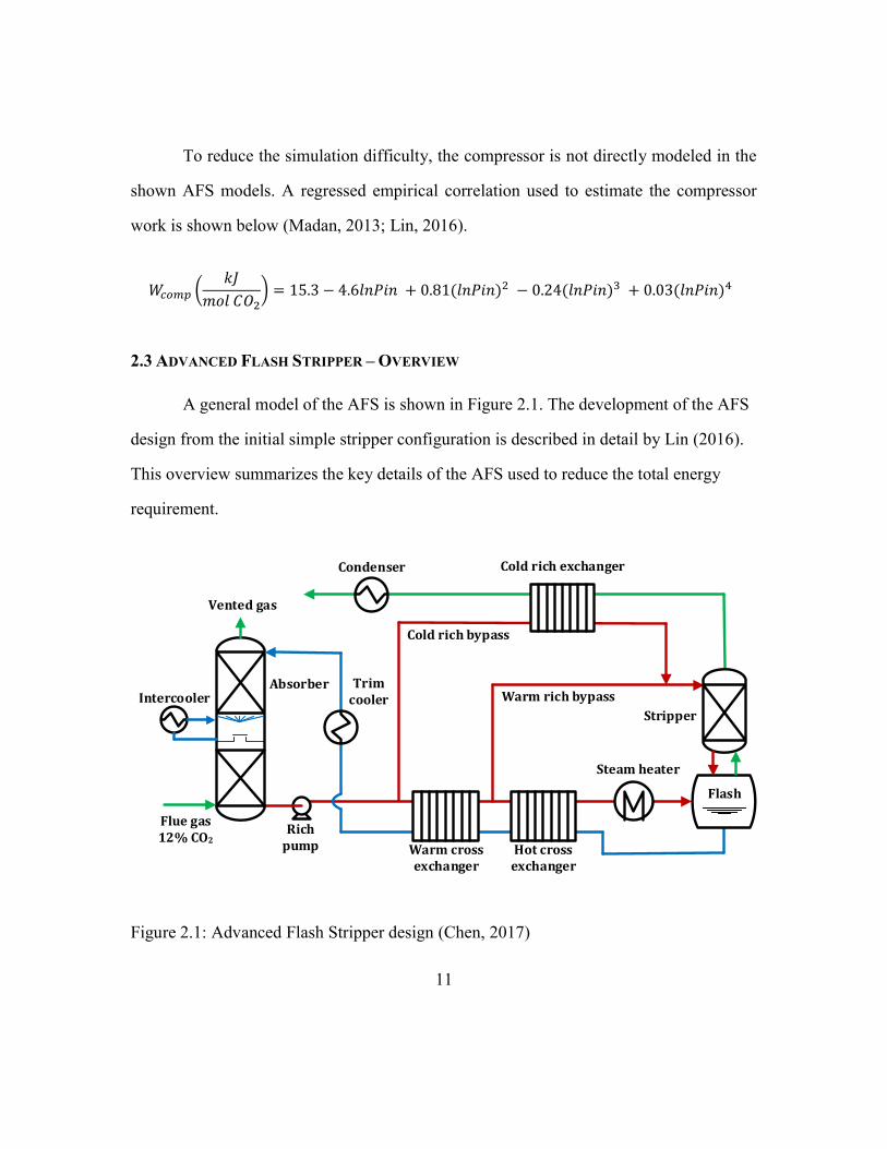
A general model of the AFS is shown in Figure 2.1. The development of the AFS
design from the initial simple stripper configuration is described in detail by Lin (2016).
This overview summarizes the key details of the AFS used to reduce the total energy
requirement.
Figure 2.1: Advanced Flash Stripper design (Chen, 2017)
Stripper
Cold rich bypass
Steam heater
Condenser Cold rich exchanger
Warm rich bypass
Flash
Warm cross exchanger
Hot cross exchanger
IntercoolerAbsorber
Flue gas12% CO2
Trim cooler
Richpump
Vented gas
12
The simple stripper design uses a single rich stream heated in a single cross
exchanger, then fed to the top of the stripper with a reboiler at the bottom heated with
steam. The advanced flash stripper separates the cross exchanger into cold and warm
exchangers, with a rich solvent bypass stream before each exchanger. The warm bypass
stream contains between 25-45% of the rich solvent and is fed to the top of the stripper,
with the balance fed to a steam heater at the bottom of the stripper that heats the solvent
to the operating temperature. The cold bypass stream strips water from the vapor inside
the stripper, reducing the water content in the hot vapor outlet to reduce energy loss in the
condenser. The temperature of the warm bypass must be selected to minimize energy
usage, as high temperatures increase the hot vapor water content, but low temperatures
require additional steam duty to heat the solvent and may lead to reabsorption of CO2 at
the top of the stripper. Previous modeling has determined the solvent bubble point as the
optimal bypass temperature (Lin, 2016). This design limits all rich solvent flashing to the
warm cross exchanger, with the cold cross exchanger transferring only sensible heat.
The cold bypass makes up a smaller portion of the rich solvent, between 2-10% of
the total rich flow. The cold bypass is used to recover heat in the cold rich exchanger
from the hot vapor containing CO2 and water (Van Wagener, 2011). The cold rich
exchanger provides additional heat recovery for the AFS, including the heat of
vaporization of water. The cold bypass receives no heat transfer from either cross
exchanger, so the benefits of heat recovery from the hot vapor must be balanced with the
heat recovery from the hot lean solvent. The heated cold bypass is combined with the
warm bypass to form a single bypass stream that enters the top of the stripper.

13
The reboiler from the simple stripper is replaced with a steam heater followed by
a flash tank to reduce solvent residence time and reduce oxidative degradation. The rich
solvent separates into two streams: a hot vapor containing water and CO2 and a lean
solvent with the lean loading determined by the operating temperature and pressure.
While the rich solvent has been effectively stripped in the flash tank, the hot vapor
contains a large mole fraction of water. The sensible and latent heat of the water vapor, if
not recovered, will be lost in the condenser which reduces the gas temperature to 40 ℃
and condenses water to produce a vapor that is 99% CO2. The stripper provides direct
contact heat recovery by contacting the vapor with warm bypass solvent, while the cold
bypass exchanger provides indirect contact heat recovery with the cold rich bypass.
2.4 AFS MODEL
Figure 2.2 shows the advanced flash stripper modeled in Aspen Plus®. While the multi-
stage compressor is not included in the model, the compressor work is estimated based on
the correlation given in section 2.2.2 and used in the calculation of equivalent work.

14
Figure 2.2: Advanced Flash Stripper Aspen Plus® model
The following sections describe how the individual unit operations of the AFS are
modeled in Aspen Plus®, including design specifications.
2.4.1 Cross exchangers
2.4.1.1 Exchanger – simplified design
For the two cross exchangers and the cold bypass exchanger, each exchanger is
modeled as a pair of heater blocks with a connecting heat stream. This is done to reduce
the difficulty of model convergence compared to the more complex MHeatX block which
provides a more complete analysis of the temperature change within the heat exchanger.
Each heater block requires two specifications out of four options: outlet temperature,
pressure drop, heat duty, or temperature change. The direction of the heat stream arrow is
nontrivial when modeling the exchanger; the heat duty of the second heater block is equal
15
and opposite the duty of the first heater block, removing one degree of freedom. As an
example, in Figure 2 the rich-end heater temperature and pressure drop are specified for
the cold and warm heater blocks, with the heat duties specified for the lean-end heater
blocks.
2.4.1.2 Heat transfer coefficient
While the double heater block method is simpler to converge, UA is not directly
calculated unlike the MHeatX method. Setting the UA for the double heater block
method in Aspen Plus® is done in two parts. First, a calculator block is used to calculate
the log mean temperature difference (LMTD) for the two heater blocks, then determine
the UA based on the specified or calculated heat duty. The same calculator block is also
used to determine the correct UA based on correlations for the heat exchanger based on
the solvent flow. Second, a design specification is used to match the actual UA to the
correct UA by varying the outlet temperature or heat duty. If the heat duty or outlet
temperature is overestimated, it is possible for the hot rich stream to exit at a higher
temperature than the hot lean stream, which is not possible in reality. This causes the
LMTD to be calculated as infinity, causing the simulation to throw an error. To prevent
this, the initial guess of the exchanger heat duty must be underestimated to guarantee a
feasible initial UA which can be improved with multiple iterations.
16
2.4.2 Steam heater and Flash Tank
The steam heater and flash tank are modeled as a single flash block with the
stripper operating temperature specified. The flash block can be modeled with one of two
configurations: the simplified model and the high temperature model shown in Figure 2.
In the simplified model, the stripper bottoms product feeds directly into the flash
tank, which then provides a single lean solvent stream at the operating temperature. This
method assumes perfect heat transfer between the hot rich feed and the hot lean bottoms,
and the temperature of the vapor outlet to the bottom of the stripper is exactly the
operating temperature. This method only includes a single operating temperature for the
stripper sump, but does not reflect the realities of the actual steam heater configuration.
Not only do the temperatures in the stripper sump not reach equilibrium, the rich solvent
must be heated above the operating temperature since the lean solvent exiting the stripper
is several degrees colder than the sump.
The high temperature model accounts for the variation in temperature within the
sump by instead modeling the lean solvent using two streams: one exiting the flash tank
and one exiting the stripper. The two streams are then mixed together to form the actual
lean solvent flow, which is fed through the cross exchangers for heat recovery. The
mixed stream is assumed to be at the operating temperature, an average of the hotter flash
tank flow and the colder stripper flow. The temperature of the flash tank is determined
using a design specification that varies the flash temperature to fit the mixed lean stream
to the operating temperature.

17
Figure 2.2: AFS stripper and flash tank, simplified model (a), high temperature model
(b).
2.4.3 Stripper column
The stripper column is modeled with a RadFracTM block with a liquid feed of
warm bypass at the top and a vapor feed of water and CO2 at the bottom. The
Independence model calculates the actual wetted area as approximately 15%, so an actual
stripper built based on the model results would need a height nearly seven times larger
than predicted by the model. The amine is stripped of CO2 primarily in the stripper sump,
with the majority of the actual column used to strip water from the vapor to increase the
CO2 mole fraction. Increasing the height of the column effectively reduces the LMTD of
the stripper, with greater heat transfer to the liquid feed. Existing Aspen Plus® models for
the AFS do not include heat loss, so the temperature of the hot vapor exiting is bounded
by the temperatures of both inputs. Chapter 4 will show how heat loss at the pilot scale
can change these results due to heat loss in the top of the stripper and the pipe length.

18
2.4.4 Lean loading
Lean and rich loading, along with the solvent rate, are defined by the absorber
performance. To achieve a specified lean loading, the temperature and pressure of the
stripper must be modified. When designing the AFS the operating temperature is selected
based on the thermal stability of the solvent, as well as the temperature of the available
steam provided at the site. Given a fixed temperature, the lean loading is controlled by
varying the stripper pressure. A design specification is used that maintains the lean
loading by controlling the pressure in the flash tank, where the majority of CO2 stripping
occurs. To correct for the changing pressure, the pump pressure is recalculated based on
the stripper pressure and any pressure drop through the main cross exchangers to provide
the required discharge pressure.
2.5 ENERGY BALANCE
A full energy balance was developed for the pilot plant data shown in Chapter 4.
The energy balance includes the inlet rich stream, outlet rich stream, CO2 product and
water condensate, steam, and cooling water. The rich solvent molality and rich loading
were calculated based on the solvent density and viscosity, and was assumed to be
accurate for the balance. The product flow was assumed to be pure CO2 and measured
with a flowmeter. A flowmeter for the liquid condensate existed, but did not provide
accurate readings. To maintain the material balance, the lean solvent composition and
flowrates were calculated based on the previous three streams. Aspen Plus® was used to
calculate the enthalpy of each stream based on the given flowrates, temperatures,

19
pressures, and compositions. A summary of the energy balance results for the NCCC
pilot plant campaign is given in Chapter 4.

20
Chapter 3: NO2 Removal using Sulfite
3.1 INTRODUCTION
NO2 impurities in flue gas may react with amines used in post combustion carbon
capture to form nitrosamines. The formation of nitrosamines degrades the amine solvent,
requiring makeup solvent and additional operating costs. While nitrosamine accumulation
in the stripper can be limited using high operating temperatures and thermal reclaiming
(Fine, 2015), neither method prevents the initial amine degradation from occurring, and
both still require the disposal of oxidized byproducts. One low-cost solution takes
advantage of the existing SO2 polisher used to capture 99% of SO2 in the flue gas. The
formula for SO2 absorption in the polisher is shown in Equation 1.
𝑆𝑂 + 2𝑂𝐻 → 𝑆𝑂 + 𝐻 𝑂 (1)
NO2 reacts with sulfite to form nitrite and sulfite free radicals (Equation 2), which
in the presence of oxygen can cause a chain reaction forming multiple free radicals that
eventually oxidize to sulfate or dithionate (Equations 3-6). This reaction occurs in the
liquid boundary layer in the polisher and the reaction mechanisms were originally
determined by Nash (1979) and Huie and Neta (1984).
𝑁𝑂 + 𝑆𝑂 → 𝑁𝑂 + 𝑆𝑂• (2)

21
𝑆𝑂• + 𝑂 → 𝑆𝑂• (3)
𝑆𝑂• + 𝑆𝑂 → 𝑆𝑂• + 𝑆𝑂 (4)
𝑆𝑂• + 𝑆𝑂 → 𝑆𝑂• + 𝑆𝑂 (5)
2𝑆𝑂• → 𝑆 𝑂 (6)
Due to the formation of additional free radicals, multiple moles of sulfite are
oxidized to capture a single mole of NO2. To reduce the sulfite oxidation, an alternate
reaction mechanism using thiosulfate as a free radical inhibitor was proposed by Owens
(1984).
𝑆𝑂• + 𝑆 𝑂 → 𝑆 𝑂• + 𝑆𝑂 (7)
𝑆𝑂 + 𝑆𝑂 → 2𝑆𝑂 (8)
𝑆 𝑂• + 𝑆 𝑂• → 𝑆 𝑂 (9)
To determine the feasibility of sulfite absorption with thiosulfate inhibitor for NO2
absorption, experiments were carried out at the National Carbon Capture Center using
coal-fired flue gas containing 40 ppm SO2 and their existing SO2 prescrubber with a 99%
removal rate. This chapter covers the results of scrubbing 1-5 ppm NO2 from flue gas,
including the sulfite oxidation rate and the benefits of thiosulfate as a free radical
scavenger.

22
3.2 EXPERIMENTAL METHODS
The pilot plant testing of the SO2 polisher for NO2 scrubbing was carried out
using a 1300-gallon polishing scrubber with 9000 lb/hr of coal flue gas containing 12%
CO2, 7% O2 and 40 ppm SO2. Solvent was constantly circulated between the scrubber and
a buffer tank at 1500 lb/hr, which was used for the addition of chemicals and solvent
bleeding. Figure 3.1 shows a simplified drawing of the scrubber and buffer tank,
including chemical addition and disposal. The pH was maintained between 7.5 and 10
using sodium hydroxide. The pH in the scrubber varied significantly due to intermittent
addition of 10 wt% NaOH when the pH decreased below 8. The SO2 in the flue gas was
converted first to sulfite and subsequently oxidized to sulfate, with 99% SO2 removal.
Figure 3.1: Process Flow Diagram of SO2 polishing scrubber

23
The buffer tank level increased during the pilot plant campaign due to water
condensation from the flue gas, which diluted the added sulfite and thiosulfate. The tank
level was initially reduced to 30% when adding sulfite, thiosulfate, and EDTA, and
maintained below 80%. The campaign was conducted in two parts. For the first week,
flue gas was used containing 0-1 ppm NO2 with no additives. For the following five
weeks, supplemental NO2 was added to the flue gas to increase the concentration to 3-5
ppm NO2. The variation in flue gas concentration was due to the valve used to maintain
the supplemental NO2 flowrate, which was based on average flue gas flowrate and not
controlled based on specific concentration.
Solid sodium sulfate, sodium thiosulfate pentahydrate, and EDTA were all
purchased from Fischer Scientific and dissolved in water before adding to the buffer tank.
After measuring the concentrations of the unmodified prescrubber solvent, the sulfite was
increased to 22 mmol/kg, thiosulfate to 120 mmol/kg, and EDTA to 0.02 mmol/kg.
Before adding the supplemental NO2 after the first week of operation, additional
thiosulfate was added to a concentration of 230 mmol/kg.
During the campaign, liquid samples were collected approximately once per day,
with additional samples taken while adding chemicals. Samples were immediately mixed
with 35 wt % formaldehyde at a ratio of 2 g formaldehyde / 10 g sample to completely
react all sulfite to form methylsulfonic acid. The samples were shipped to Austin for
additional analysis. To determine the rate of sulfite and thiosulfate oxidation, the liquid
samples were analyzed using anion chromatography. The anion chromatography method
and the bench-scale testing apparatus are both described in Appendix A.

24
3.3 RESULTS
3.3.1 Sulfite
The initial addition of thiosulfate significantly reduced oxidation within the
prescrubber tank, leading to a net increase in sulfite over the first week of operation.
During the first three days of operation, sulfite increased from 22 mmol/kg to 53
mmol/kg. Thiosulfate decreased over the first week due to both reacting with sulfite
radicals and tank dilution due to water condensation in the flue gas. As thiosulfate
decreased below 90 mmol/kg, the sulfite concentration reached a maximum at 52
mmol/kg, then decreased to 45 mmol/kg over the remainder of week 1.
During weeks 2-6, sulfite loss was first order with respect to sulfite as shown in
Figure 3.2. The rate constant was 3.0 hr-1, more than an order of magnitude greater than
previous bench-scale experiments with rate constants of 50-400 hr-1 (Sexton 2018). The
reduced rate constant was due to the feed of 40 ppm SO2 in the flue gas, producing a
constant sulfite feed that was unaffected by the concentration of either sulfite or
thiosulfate.
25
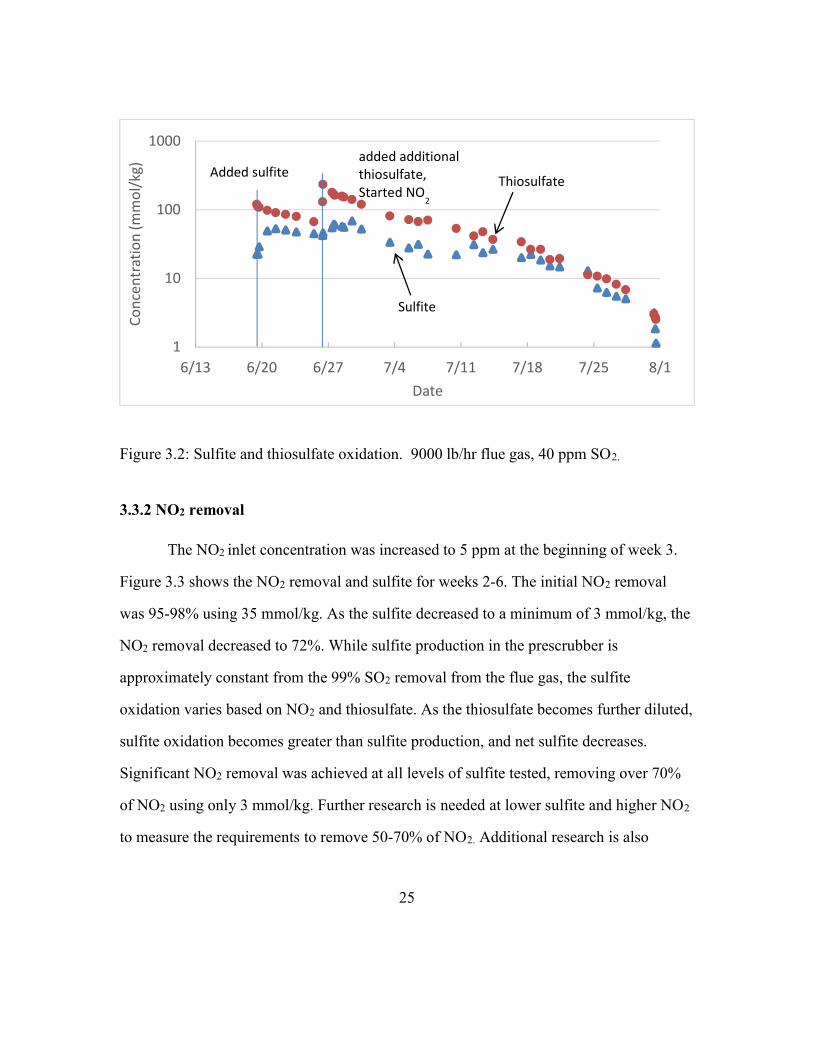
Figure 3.2: Sulfite and thiosulfate oxidation. 9000 lb/hr flue gas, 40 ppm SO2.
3.3.2 NO2 removal
The NO2 inlet concentration was increased to 5 ppm at the beginning of week 3.
Figure 3.3 shows the NO2 removal and sulfite for weeks 2-6. The initial NO2 removal
was 95-98% using 35 mmol/kg. As the sulfite decreased to a minimum of 3 mmol/kg, the
NO2 removal decreased to 72%. While sulfite production in the prescrubber is
approximately constant from the 99% SO2 removal from the flue gas, the sulfite
oxidation varies based on NO2 and thiosulfate. As the thiosulfate becomes further diluted,
sulfite oxidation becomes greater than sulfite production, and net sulfite decreases.
Significant NO2 removal was achieved at all levels of sulfite tested, removing over 70%
of NO2 using only 3 mmol/kg. Further research is needed at lower sulfite and higher NO2
to measure the requirements to remove 50-70% of NO2. Additional research is also
1
10
100
1000
6/13 6/20 6/27 7/4 7/11 7/18 7/25 8/1
Conc
entr
atio
n (m
mol
/kg)
Date
Added sulfite added additional thiosulfate, Started NO
2
Sulfite
Thiosulfate

26
needed at reduced oxygen concentrations, which will further reduce the oxidation rate
while not affecting sulfite production from SO2.
Figure 3.3: NO2 removal decreases as sulfite oxidizes.
3.3.3 pH
As seen in Figure 3.3, NO2 removal showed a clear cyclical trend, with an
average period of 4 days. Figure 3.4 once again shows the NO2 removal, now compared
to pH. An increase in pH is immediately followed by an increase in removal that decays
as the pH drops below 8. Increasing the pH by 1.5 points improves NO2 removal by 5-
8%, which was not correlated with sulfite or thiosulfate concentrations.
0
5
10
15
20
25
30
35
40
70%
75%
80%
85%
90%
95%
100%
6/29 7/6 7/13 7/20 7/27 8/3
Sulfi
te (m
mol
/kg)
NO
2re
mov
al
Date
NO2
Removal
Sulfite
27
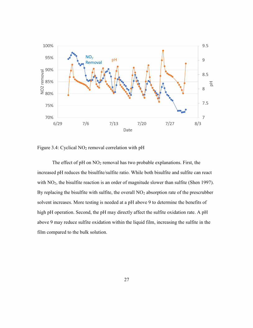
Figure 3.4: Cyclical NO2 removal correlation with pH
The effect of pH on NO2 removal has two probable explanations. First, the
increased pH reduces the bisulfite/sulfite ratio. While both bisulfite and sulfite can react
with NO2, the bisulfite reaction is an order of magnitude slower than sulfite (Shen 1997).
By replacing the bisulfite with sulfite, the overall NO2 absorption rate of the prescrubber
solvent increases. More testing is needed at a pH above 9 to determine the benefits of
high pH operation. Second, the pH may directly affect the sulfite oxidation rate. A pH
above 9 may reduce sulfite oxidation within the liquid film, increasing the sulfite in the
film compared to the bulk solution.

28
3.3.4 Tank level
Due to condensed water in the flue gas, the liquid level in the prescrubber tank
increased by 2-4% per day. Figure 3.5 shows the tank level in percent during the
campaign, including multiple solution bleeds. The tank level was initially reduced to 30%
at the beginning of week 1 while adding chemicals, then reduced to 30% again at the
beginning of week 3. Instead of a constant solution bleed from the tank, the level was
maintained by large intermittent bleeds to maintain a specific level. After adding
chemicals at the beginning of week 2, the level was allowed to increase to 80%. The level
was maintained between 60% and 80% for the remainder of the campaign. Additional
spikes in level occurred when sodium hydroxide was added to maintain a pH over 8. The
sulfate concentration was controlled by both solvent dilution and the intermittent bleeds.
Figure 3.5: Prescrubber tank level and bleed
0102030405060708090
6/17 6/24 7/1 7/8 7/15 7/22 7/29 8/5
Tank
Lev
el (%
)
Date

29
The loss of thiosulfate was due to both reactions with free radicals and tank
bleeds. Figure 3.6 shows the total moles of thiosulfate from weeks 2-5. The prescrubber
solution lost 260 moles of thiosulfate over 750 hours, with 60 moles of the loss attributed
to solution disposal. An average of 0.27 mol/hr of thiosulfate was lost due to oxidation,
accounting for over 75% of thiosulfate lost. For the given flue gas feed of 9000 lb/hr with
5 ppm NO2, the replenishment rate for thiosulfate is 0.4 mol / mol NO2. This corrsponds
apporximately to the stoichiometry:
2 S2O32- + 2 NO2 ↔ 2 S2O3
- + 2 NO2-
2 S2O3- ↔ S4O6
2-
S4O62- + SO3
2- ↔ S3O62- + S2O3
2-
Overall:
S2O32- + 2 NO2 + SO3
2- ↔ 2 NO2- + S3O6
2-
Figure 3.6: Total thiosulfate losses.
0
50
100
150
200
250
300
0 100 200 300 400 500 600 700 800
Thio
sulfa
te (m
oles
)
Hours

30
3.3.5 Removal requirements
In order to maintain a constant 90% removal of NO2, the sulfite concentration
must be maintained by reducing the oxidation rate below the rate of sulfite addition from
flue gas SO2. Varying thiosulfate adjusts the steady-state concentration of sulfite in the
prescrubber, requiring makeup thiosulfate which was not tested in this campaign. Figure
3.7 shows a power law correlation between the thiosulfate concentration and the steady-
state concentration of sulfite. The correlation was developed using a thiosulfate range
from 5 to 180 mmol/kg. Doubling the thiosulfate increases sulfite by a factor of 1.6. The
correlation is dependent on both SO2 and NO2 in the flue gas. Increasing SO2 increases
the rate of sulfite production and reduces the required thiosulfate, while NO2 increases
sulfite oxidation and requires additional thiosulfate. The effects of total gas flow are
mixed, as additional NO2 may lead to a rapid spike in sulfite oxidation. The correlation
also assumes O2 at 5-7%, which plays a key role in propagating the sulfite free radical
reactions. The effects of reducing the O2 below 5% are unclear: Shen predicted a
proportional reduction in oxidation with O2 concentration, while Fine predicted the
oxidation rate would only decrease below 5% as the liquid boundary layer is depleted of
oxygen. Bench-scale experiments conducted by Sexton et al. corroborate Shen, as
reducing oxygen from 21% to 8% significantly reduced the oxidation rate.

31
Figure 3.7: Steady-state sulfite correlation with thiosulfate, 40 ppm SO2, 5 ppm NO2.
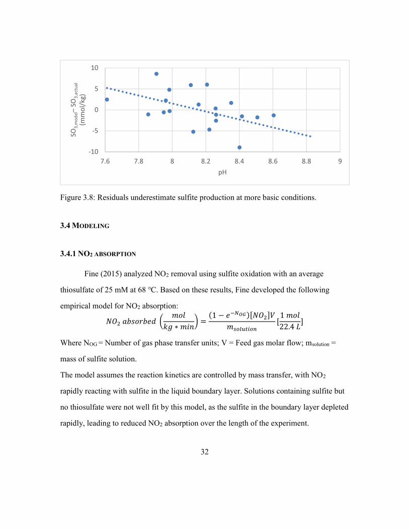
The data in Figure 3.7 were collected at an average pH of 8.2, but actual pH
varied from 7.5 to 9.5. As discussed previously, pH directly correlated with increased
NO2 removal regardless of sulfite and thiosulfate concentrations. Figure 3.8 shows the
residuals of the sulfite-thiosulfate correlation correlated with pH. The correlation
overestimates sulfite at low pH, and underestimates sulfite at high pH. The additional
residual correlation suggests high pH significantly reduced sulfite oxidation. By
increasing the pH in the prescrubber, a higher concentration of sulfite can be achieved
without increasing thiosulfate.
32
Figure 3.8: Residuals underestimate sulfite production at more basic conditions.
3.4 MODELING
3.4.1 NO2 ABSORPTION
Fine (2015) analyzed NO2 removal using sulfite oxidation with an average
thiosulfate of 25 mM at 68 ℃. Based on these results, Fine developed the following
empirical model for NO2 absorption:
𝑁𝑂 𝑎𝑏𝑠𝑜𝑟𝑏𝑒𝑑 𝑚𝑜𝑙
𝑘𝑔 ∗ 𝑚𝑖𝑛=
(1 − 𝑒 )[𝑁𝑂 ]𝑉
𝑚[1 𝑚𝑜𝑙
22.4 𝐿]
Where NOG = Number of gas phase transfer units; V = Feed gas molar flow; msolution =
mass of sulfite solution.
The model assumes the reaction kinetics are controlled by mass transfer, with NO2
rapidly reacting with sulfite in the liquid boundary layer. Solutions containing sulfite but
no thiosulfate were not well fit by this model, as the sulfite in the boundary layer depleted
rapidly, leading to reduced NO2 absorption over the length of the experiment.
-10
-5
0
5
10
7.6 7.8 8 8.2 8.4 8.6 8.8 9
SO3,
mod
el–
SO3,
actu
al(m
mol
/kg)
pH
33
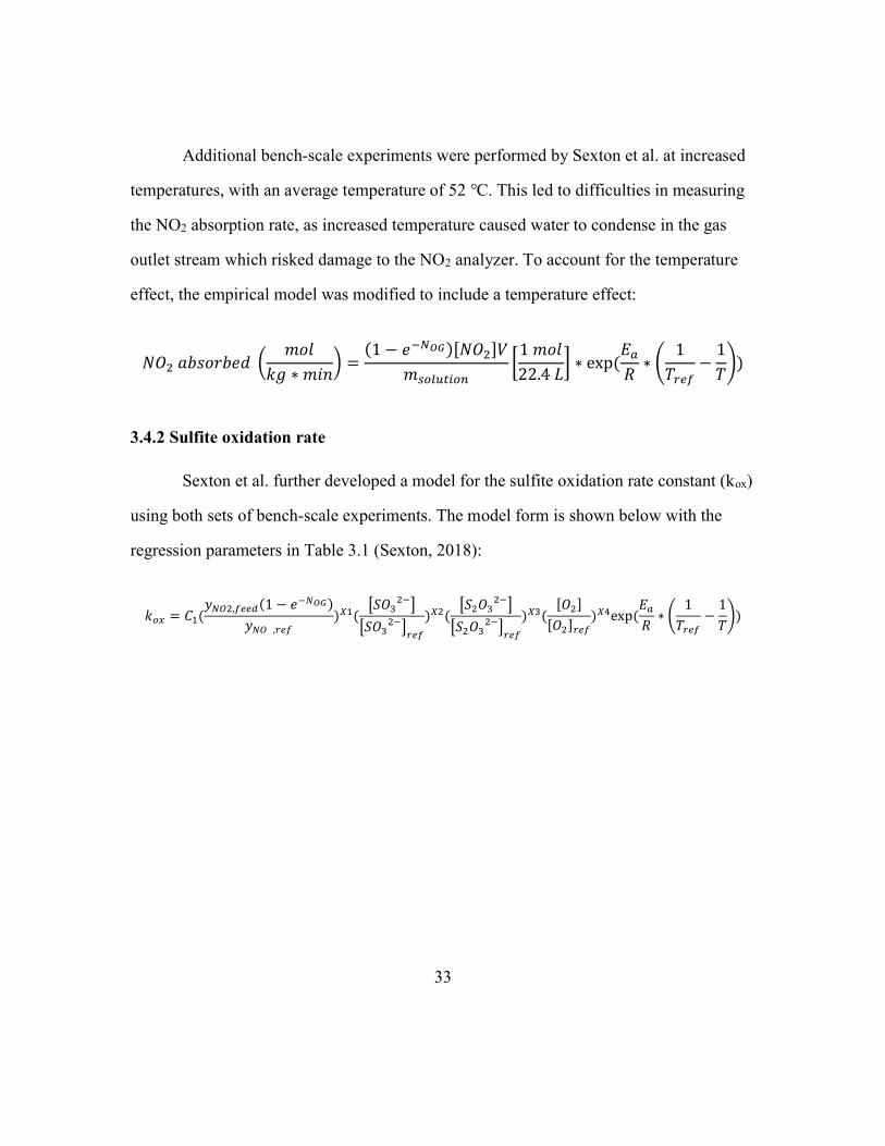
Additional bench-scale experiments were performed by Sexton et al. at increased
temperatures, with an average temperature of 52 ℃. This led to difficulties in measuring
the NO2 absorption rate, as increased temperature caused water to condense in the gas
outlet stream which risked damage to the NO2 analyzer. To account for the temperature
effect, the empirical model was modified to include a temperature effect:
𝑁𝑂 𝑎𝑏𝑠𝑜𝑟𝑏𝑒𝑑 𝑚𝑜𝑙
𝑘𝑔 ∗ 𝑚𝑖𝑛=
(1 − 𝑒 )[𝑁𝑂 ]𝑉
𝑚
1 𝑚𝑜𝑙
22.4 𝐿∗ exp (
𝐸
𝑅∗
1
𝑇−
1
𝑇)
3.4.2 Sulfite oxidation rate
Sexton et al. further developed a model for the sulfite oxidation rate constant (kox)
using both sets of bench-scale experiments. The model form is shown below with the
regression parameters in Table 3.1 (Sexton, 2018):
𝑘 = 𝐶 (𝑦 , (1 − 𝑒 )
𝑦 ,
) (𝑆𝑂
𝑆𝑂) (
𝑆 𝑂
𝑆 𝑂) (
[𝑂 ]
[𝑂 ]) exp (
𝐸
𝑅∗
1
𝑇−
1
𝑇)

34
Table 3.1: Regression parameters from oxidation model (Sexton, 2018)
Parameter Regressed Model
C1 7.30
Ea (kJ/mol) 23.8
X1 (Nitrite) 0.55
X2 (Sulfite) -0.05
X3 (Thiosulfate) -0.39
X4 (Oxygen) 0.18
The expanded empirical model includes all relevant process variables expected to affect
sulfite oxidation. Of particular interest is the limited effect of thiosulfate and oxygen
found in the model. This is due to the majority of data using a minimum of 25 mM
thiosulfate and 4% oxygen. While inhibited sulfite solutions reduce the number of moles
of sulfite oxidized / mole of NO2 absorbed by an order of magnitude compared to
uninhibited solutions, there are rapidly diminishing returns with additional thiosulfate. A
similar effect is seen for oxygen, with very low (<4%) O2 in the feed gas significantly
reducing sulfite oxidation which is not seen in the existing data set.
3.5 ALTERNATIVE INHIBITOR METHODS
The estimated cost of thiosulfate pentahydrate is $0.70/lb. Two alternative
methods have been considered for further reducing this cost. The first method is direct

35
production of thiosulfate from colloidal sulfur. The reaction of sulfur with sulfite to
produce thiosulfate is as follows:
S + SO32-
→ S2O32-
Initial testing using sulfur to produce thiosulfate have shown over 90% yield within 24
hours of addition, though sufficient agitation is needed to ensure the sulfur does not settle
to the bottom of the vessel. Using sulfur may require a large initial feed of sulfite and
thiosulfate to the prescrubber during start-up to ensure the reaction proceeds while NO2 is
absorbed. Without an initial feed of thiosulfate, the sulfite will oxidize to sulfate rather
than react with the sulfur. To reach steady-state, the sulfite-thiosulfate correlation must be
used to maintain the sulfite while the sulfur reacts with sulfite to produce more thiosulfate
and further inhibit oxidation.
In design cases where the SO2 feed is low, there may not be sufficient sulfite
produced to effectively remove NO2 regardless of inhibitor quantity. While NO2 removal
can still be conducted in the prescrubber, an alternate non-sulfite inhibitor is required.
Fine showed tertiary amines provide effective oxidation inhibition by preferentially
reacting with NO2. Unlike sulfite, tertiary amines are not affected by oxygen-rich flue
gas, providing additional benefits.

36
Chapter 4: NCCC Advanced Flash Stripper Testing
4.1 INTRODUCTION
Demonstrating the effectiveness of novel stripper configurations and solvents
requires not only process modelling but also experimental results at the pilot scale. The
pilot plant at the UT Austin Separations Research Program (SRP) has tested a variety of
design configurations using piperazine, including the simple stripper, 1- and 2-stage flash
with cold bypass, and the advanced flash stripper (Van Wagener, 2011; Lin, 2016; Chen,
2017). SRP completed two pilot plant campaigns using piperazine and the AFS; first in
2015 using 5m and 8m PZ and a flue gas containing 12% CO2, then again in 2017 using
5m PZ and flue gas ranging from 4% to 20% CO2. The SRP campaign results from 2015
have been discussed in depth by Lin, Chen, and Rochelle (2016), and the 2017 campaign
results have been analyzed by Chen et al. (2017). The results from the NCCC pilot plant
in this chapter have been previously published (Selinger, 2018).
4.2 AFS TESTING – SRP
The initial SRP test of the AFS was the first test of the new configuration, and
showed reduced heat duty compared to previous designs and the benefits of a less viscous
solvent on heat transfer. Figure 4.1 shows the reboiler heat duty of the 2015 SRP testing
compared to previous tests over the past five years. The AFS showed a reduction of heat
duty by 25% compared to the simple stripper, with heat duty ranging from 2.1-2.9 GJ/MT
CO2. Varying the cold and warm bypasses also determined that optimization of the
bypass percentages could reduce heat duty by 5-15% (Lin, 2014).

37
Figure 4.1: Comparison of heat duty between SRP tests
The SRP campaign in 2017 continued testing with the AFS configurations, now
only using 5m PZ. Testing included three concentrations of CO2 in the flue gas
representing three design cases: 3.5% to represent natural gas-fired turbines, 12% for
coal-fired power plants, and 20% for a new hybrid process combining membranes with
amine scrubbing to produce a flue gas with increased CO2 percentage. Since the stripper
operating conditions are defined by the rich loading, lean loading, and solvent flowrate,
the inlet CO2 does not directly affect performance. However, reduced inlet CO2 requires a
lower lean loading and increased solvent flowrate to achieve the desired removal rate,
which increases the required heat duty of the stripper.

38
Figure 4.2 shows the performance of the SRP 2017 AFS compared to test cases
modeled in Aspen Plus®. Lean loading was strongly correlated with heat duty, with an
average delta loading of 0.15. Reducing the lean loading from 0.24 to 0.18 while
maintaining a constant AFS operating temperature of 150 ℃ required reducing the
stripper pressure from 5.4 barg to 4.1 barg. The reduced pressure in the stripper reduces
the CO2 to water ratio in the stripper due to the changes in the heat of vaporization of
water compared to the heat of desorption of CO2. As the water content in the hot vapor
exiting the stripper increases, more energy is lost in the condenser removing condensate,
leading to increased overall energy costs.
Figure 4.2: Heat duty of SRP 2017 compared to test cases
The test plan cases showed an average heat duty approximately 20% less than the
actual pilot plant results. This difference includes the estimated heat loss of the stripper,

39
with increased solvent flowrates leading to increased heat loss. The heat loss as a
percentage of total duty is expected to reduce as the process is further scaled-up to
commercial size. In addition to heat loss, the model may have underestimated the energy
requirements by underestimating the heat of desorption of 5 m PZ. A low heat of
desorption solvent requires less energy to strip the CO2 from the rich solvent, so the total
energy requirement would be underestimated.
4.3 NCCC METHODS
4.3.1 NCCC vs SRP
The remainder of this chapter covers the testing completed at the National Carbon
Capture Center (NCCC) pilot plant conducted between February to August 2018. The
NCCC pilot plant is connected to the Gaston coal-fired power plant in Wilsonville,
Alabama, which provided a fraction of the flue gas produced by an 880 MW coal boiler
to the pilot plant. The NCCC pilot plant provided two key benefits compared to the SRP
pilot plant testing previously completed. First, the flue gas directly represents the
conditions of flue gas from a commercial coal plant, including trace NOx, SOx, and
particulate. The SRP pilot plant uses a synthetic flue gas made up of air and CO2, with
SO2 injected during some runs to test the formation of aerosols. Second, the NCCC plant
provides an increased flowrate of flue gas, equivalent to 0.5 MW compared to SRP’s 0.1
MW. Table 4.1 summarizes the differences between the NCCC design and the SRP
design.

40
Table 4.1: Comparison of NCCC and SRP advanced flash stripper designs
NCCC SRP
Stripper diameter (in) 10 10
Stripper height (m) 4 2.25
Packing material RSR 0.5, 0.7 RSR 0.5
Flue gas origin Coal plant Synthetic
Flue gas rate 0.5-0.6 MW 0.1 MW
4.3.2. Measurements
Data was collected from all instruments once per minute, and averaged over
steady-state periods to define individual runs. CO2 product flow was measured using a
CO2 flowmeter, though some data was lost due to intermittent plugging of the flow meter.
The product flow was also estimated using the rich solvent flow, PZ molality, and delta
loading. Molality and loading were calculated based on density, viscosity, and
temperature using a regressed model for PZ loading (Freeman, 2011; Zhang et al., 2017).
Due to a broken viscosity measurement on the lean stream, both molality and loading
could not be directly determined for the lean return solvent. To calculate lean loading, the
molality was assumed identical to the rich molality, and loading was calculated using
only the density of piperazine. The density-viscosity correlation is listed below:

41
= ∗ (0.0407 ∗ 𝐶 + .0008 ∗ 𝐶 + .991)
µ = µ ∗ exp [26.16
𝑇− .0265 ∗ (7.69 ∗ 𝐶 − 7.80 ∗ 𝐶 + 3.37 ∗ 𝐶 ∗ 𝐶 )]
µ = 2.41 ∗ 10 ∗ 10 . /( )
= density (kg/m3); = viscosity PZ (cP); C = concentration (mol/kg); T = temperature
(K)
Given density, viscosity, and temperature, the correlation system of equations can be
solved.
4.4 NCCC TEST CASE MODELING
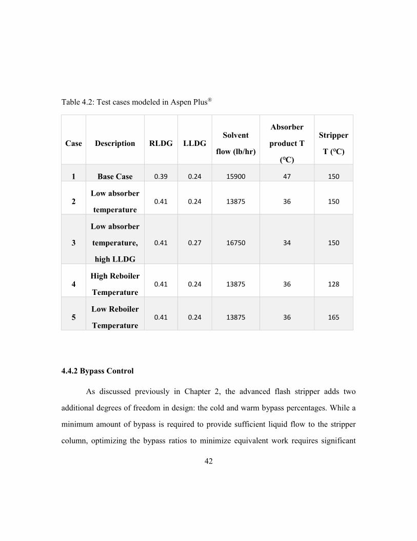
4.4.1 Test case plan
Before starting the NCCC campaign, test cases were simulated in Aspen Plus® to
estimate the equivalent work and optimize the bypasses based on the Independence
model. Table 4.2 lists five test cases analyzed, representing a range of conditions to be
tested during the campaign. Case 1 represents the base case, with a lean loading of 0.24
and an operating temperature at 150 ℃. Cases 2 and 3 reduce absorber temperature by 7
℃, which increases the CO2 mass transfer driving force and requires less solvent to
capture 90% of CO2 in the flue gas. Cases 4 and 5 test the effects of stripper operating
temperature between 128 ℃ to 165 ℃, directly increasing pressure along with
temperature to maintain lean loading.
42
Table 4.2: Test cases modeled in Aspen Plus®
Case Description RLDG LLDG Solvent
flow (lb/hr)
Absorber
product T
(℃)
Stripper
T (℃)
1 Base Case 0.39 0.24 15900 47 150
2 Low absorber
temperature 0.41 0.24 13875 36 150
3
Low absorber
temperature,
high LLDG
0.41 0.27 16750 34 150
4 High Reboiler
Temperature 0.41 0.24 13875 36 128
5 Low Reboiler
Temperature 0.41 0.24 13875 36 165
4.4.2 Bypass Control
As discussed previously in Chapter 2, the advanced flash stripper adds two
additional degrees of freedom in design: the cold and warm bypass percentages. While a
minimum amount of bypass is required to provide sufficient liquid flow to the stripper
column, optimizing the bypass ratios to minimize equivalent work requires significant
43
testing to determine and varies with changes to any process variable. While model
optimization can be completed through multiple simulations, real-world testing is limited
and an alternate heuristic must be developed to rapidly identify optimal or near-optimal
bypass percentages.
Alternative process controls methods for the AFS were studied by Matt Walters
(2016). Analyses of process control methods identify the temperature differences
between hot vapor exiting the stripper and the bypass streams as process variables that
can be controlled to minimize heat duty. Rather than set the mass flowrates for each
bypass stream, the temperature differences would be specified and the mass flowrates
controlled. One advantage of this method is the automatic readjustment of bypass
flowrates as process changes are made, though this was not implemented in the design of
the NCCC pilot plant. The temperature differences are referred to as DT1 and DT2 for
the cold and total bypass streams. Figure 4.3 shows the temperature differences used for
process control.

44
Figure 4.3: Temperature differences used to optimize bypass: DT1 (blue), DT2 (red)
(Walters, 2016)
The temperature differences are calculated as follows:
DT1 = Tstripper gas – TCX3 Cold Outlet
DT2 = Tstripper gas – Ttotalbypass

45
4.4.3 Test Case Results
The five test cases were modeled with two bypass calculation methods. First, each
case was optimized to minimize equivalent work. Second, DT1 and DT2 were both
assumed as 7 ℃ and the models were recalculated. Table 4.3 lists the bypass percentages
for each case when using temperature control. When using DT1 and DT2 as controls, the
mass flowrates varied significantly without the need to update the actual controls.
Table 4.3: Rich bypass controlled by temperature difference
Case Description Cold bypass (%) Warm bypass (%)
Base Case 7.8 26.9
Low absorber
temperature 7.1 32.1
Low absorber
temperature,
high LLDG
4.6 18.7
High Reboiler
Temperature 4.9 24.9
Low Reboiler
Temperature 15.8 40.1
The bypass percentages vary significantly based on solvent loading and
temperature. Both bypasses are minimized when operating at increased lean loading and
increased temperature, and maximized when reducing temperature. Overall, the bypass

46
flow is dependent on the stripper pressure, with increased pressure raising the CO2 to
water ratio in the hot vapor. With less water trapped in the hot vapor exiting the stripper,
less cold bypass is needed to recover the latent heat of steam.
Figure 4.4 compares the equivalent work from the temperature control cases to
the actual optimized results. All temperature control cases showed similar performance to
the optimized results, with the largest differences due to variations in operating
temperature. While these tests suggest temperature control as a viable heuristic, the
method is limited by several factors. First, the temperatures measured assumed no heat
loss, which reduce temperature differences. Second, while 7 ℃ was assumed for both
DT1 and DT2, it is not obvious these temperature differences are optimal for all process
designs. Third, the NCCC plant required the bypass flow rates to be directly set by the
operator and did not have control systems to vary the flow set points based on
temperature differences.
Figure 4.4: Equivalent work of test cases: optimized vs. temperature control
36
37
38
39
40
41
42
43
Base Case(BC)
BC, Low T BC, Low T,High LLDG
High Reb T Low Reb T
Equi
vale
nt w
ork
(kJ /
mol
CO
2) Temperature Controlled
Optimized

47
4.5 RESULTS
4.5.1 Experimental data collection
Data was collected from the NCCC pilot plant from January-August 2018, with
several shutdowns due to repairs or reduced demand. After initial water testing, 600
hours of parametric testing with the AFS was completed. The simple stripper
configuration was also tested for an additional 250 hours, using only the cold cross
exchanger which limited available heat recovery. Finally, long-term testing with the AFS
was conducted for 1350 hours before shutting down. Table 4.4 summarizes the AFS
conditions tested during the campaign. Example AFS control system overview
screenshots are included in Appendix B.
Table 4.4: AFS parameter test ranges
Parameter Range
Lean Loading 0.20 – 0.27 mol/equiv PZ
Rich Loading 0.37 – 0.41 mol/equiv PZ
Solvent Flow 10000 – 20000 lb/hr
Stripper Temperature 133 - 155 ℃
Stripper Pressure 35 – 92 psig
Cold bypass flow 500 – 1500 lb/hr
Warm bypass flow 2500 – 7200 lb/hr
48
4.5.2 Data limitations
When the temperature control heuristic was used in Section 4.4 to simulate NCCC
performance, it was assumed that DT1 and DT2 would both be positive values. In a
simulated design with no heat loss, this is by definition true: the hot vapor outlet
temperature is between the temperature of the bypass and the stripper operating
temperature. However, heat loss occurring in the AFS reduced DT2 far below expected,
with an average DT2 of -4 compared to the expected value of 7 ℃. This change limited
the effectiveness of the temperature control heuristic.
Unlike the design of SRP, the temperature transmitter measuring the hot CO2
vapor (TI40503) is not placed directly near the hot vapor outlet; rather, it is placed just
before the cold bypass. Because of this difference in placement, two possible sources of
heat loss are possible: heat loss in the column and heat loss in the pipe between the
column and exchanger. If heat is lost in the column, additional water would be condensed
and the CO2 to water ratio of the vapor would increase. If heat is lost in the pipe, the
additional water exits the top of the column but condenses in the pipe before the
exchanger. Unfortunately, the flow rate of liquid condensate from the condenser was not
accurately measured, so the water loss cannot be directly determined. Regardless of the
heat loss source, the heat loss limits the benefits of heat recovery from the cold bypass
exchanger. As seen in the test cases with high lean loading, reducing latent heat in the hot
vapor reduces the required cold bypass flow.
49
4.5.3 Material Balance
The total CO2 removal of the AFS can be calculated by two methods: the flow of
product CO2 exiting the AFS and the delta loading of the solvent multiplied by molality
and solvent flow rate. Figure 4.5 shows the relative error of the measured CO2 flow rate
compared to the change in loading method over all AFS runs. The solvent and loading
method used the density-viscosity correlation to determine both rich and lean loading.
The solvent method of determining CO2 flow effectively closed the material balance,
with an average overestimate of 4%. The variation may be due to variations in the
measurement of rich solvent flow, but the consistent positive overestimation suggests the
density-viscosity correlation may require an additional multiplier to match the results to
real data.

50
Figure 4.5: Overestimation of CO2 mass balance by 4%. Relative mass balance error was
calculated as % 𝑒𝑟𝑟𝑜𝑟 = ( , , )
,. Solvent flow rate ranges
from 10000 – 20000 lb/hr.
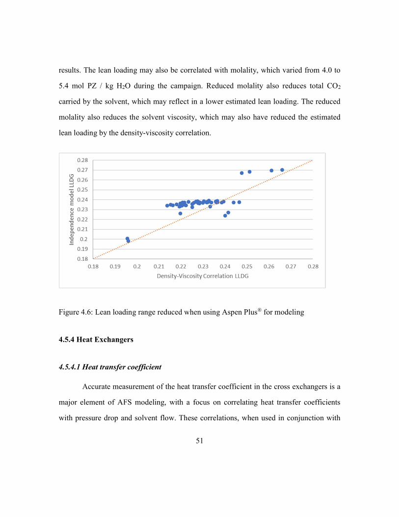
The majority of runs in the NCCC test plan included a lean loading of 0.24
mol/PZ equiv, with stripper temperature and pressure calculated to provide the desired
lean loading. The required pressure was calculated using the Independence model in
Aspen Plus®. Figure 4.6 compares the lean loading calculated by the Independence model
to the lean loading calculated by the density-viscosity correlation. While the runs at low
and high loading were similar for both methods, the correlation showed a greater
variation of lean loadings between 0.21 and 0.25 mol/PZ equiv, while the Independence
model limited the range of loadings between 0.23 and 0.24 mol/PZ equiv. It is
additionally possible another variable beyond pressure and temperature must be
considered when modelling runs, which would better match the model to match the actual
51
results. The lean loading may also be correlated with molality, which varied from 4.0 to
5.4 mol PZ / kg H2O during the campaign. Reduced molality also reduces total CO2
carried by the solvent, which may reflect in a lower estimated lean loading. The reduced
molality also reduces the solvent viscosity, which may also have reduced the estimated
lean loading by the density-viscosity correlation.
Figure 4.6: Lean loading range reduced when using Aspen Plus® for modeling
4.5.4 Heat Exchangers
4.5.4.1 Heat transfer coefficient
Accurate measurement of the heat transfer coefficient in the cross exchangers is a
major element of AFS modeling, with a focus on correlating heat transfer coefficients
with pressure drop and solvent flow. These correlations, when used in conjunction with

52
Aspen Plus®, allow for optimization of bypass rates and further testing of novel design
cases. Figure 4.7 correlates heat transfer coefficients to solvent rate for the two cross
exchangers, while Figure 4.8 does the same for the cold bypass exchanger. Both cold
exchangers directly correlated heat transfer to solvent rate, with U increasing with
average solvent rate by powers of 0.96 for the cold cross and 1.108 for the cold bypass.
The direct correlation is expected as the solvent does not flash in either cold exchanger.
All average flows for Figure 4.8 are clustered around 8 set points due to fixed solvent rate
settings used for all runs. The hot exchanger, which includes some flashing in all runs,
shows a reduced power-law correlation of 0.66, with heat transfer no longer directly
scaling with solvent flow. Flashing within the exchanger leads to nucleate boiling, which
is limited by the temperature approach.
Figure 4.7: Cross exchanger heat transfer with direct correlation for cold exchanger. Cold
cross exchanger area = 1227 ft2. Warm cross exchanger area = 207 ft2.
y = 0.0136x0.9607
R² = 0.9525
y = 0.606x0.6582
R² = 0.6848
80
130
180
230
280
330
380
430
8000 10000 12000 14000 16000 18000 20000
U (B
tu/h
r/ft
2 /℉
)
Avg flow (lb/hr)
Cold Exchanger
Warm Exchanger

53
Figure 4.8: Bypass exchanger with lower U compared to cross exchangers due to liquid-
gas exchange vs. liquid-liquid heat exchange in the cross exchangers.
Bypass exchanger area = 91.5 ft2.
4.5.4.2 Pressure drop
Selecting pressure drop in heat exchangers requires balancing heat transfer
performance with increased capital and operating costs. As solvent flow increases, the
fluid velocity causes additional turbulence within the exchanger, increasing both heat
transfer and pressure drop. The optimum fluid velocity in the cross exchanger is
dependent on the capital costs of the pump and heat exchanger as well as the cost of
steam and electricity (Lin, 2016). Figures 4.9 and 4.10 show the increased heat transfer
coefficient with respect to pressure drop for the cold and hot cross exchangers. As
previously seen in Figure 7, the hot cross exchanger correlation is less accurate than the
cold cross exchanger correlation due to flashing at high temperatures.

54
Figure 4.9: Heat transfer correlation with pressure drop for the cold cross exchanger
Figure 4.10: Heat transfer correlation with pressure drop for the hot cross exchanger
y = 68.986x0.666
R² = 0.9342
90
100
110
120
130
140
150
160
170
180
190
1.5 2.0 2.5 3.0 3.5 4.0 4.5
U (
Btu
/hr/
ft2/
℉)
Average pressure drop (psi)
y = 44.469x0.6273
R² = 0.6722
100
150
200
250
300
350
400
14 16 18 20 22 24 26 28
U (
Btu
/hr/
ft2/
℉)
Warm cross exchanger Rich dP (psi)

55
4.5.5 Heat duty
4.5.5.1 Experimental vs. model
The heat duty for the advanced flash stripper was calculated using the measured
flowrate and pressure of steam and the product flowrate of CO2 measured by flowmeter,
assuming complete condensation of steam. Figure 4.11 shows the total heat duty per
metric ton of CO2 vs. delta loading. The data shown includes the initial test plan model
results, the factorial testing, and the long-term testing at the end of the campaign lasting
six weeks. The long-term data includes measurements in the morning and afternoon to
determine the effect of ambient temperature on performance.
Figure 4.11: Model and experiment heat duty inversely correlated with delta loading
2.0
2.1
2.2
2.3
2.4
2.5
2.6
2.7
0.140 0.145 0.150 0.155 0.160 0.165 0.170 0.175 0.180
Hea
t dut
y (G
J/M
T C
O2)
DeltaLDG
Long-term Morning Long-term Afternoon Factorial Model

56
The heat duty was reduced with increased delta loading, due to a lower solvent
rate required to strip a fixed flowrate of CO2. Both factorial and long-term testing
required lower heat rates than predicted from the modeled test cases, despite heat loss not
being included in the Aspen model. Long-term morning results (07:00-08:30) showed
slightly better performance than long-term afternoon results (15:00-16:30). The lower
heat rates were partially caused by better heat transfer coefficients in the cross exchanger
compared to predictions based on previous heat exchanger performance at SRP. The
minimum heat duty required during long-term testing was 2.0 GJ/MT CO2, with an
estimated 0.2-0.3 GJ/MT CO2 of the cost due to heat loss.
4.5.5.2 Energy balance
An energy balance was performed using the Independence model over the
complete AFS to determine total heat loss. The energy balance, as previous discussed in
Chapter 2, includes the rich solvent feed, lean solvent return, CO2 product flow,
condensed water, steam inlet and outlet, and cooling water inlet and outlet. The AFS is
not modeled for the energy balance, only the enthalpy of the individual streams based on
temperature, pressure, flowrate, and loading. The total energy input to the system is from
the solvent feed, medium pressure steam, and cooling water inlet. As expected, the outlet
components of the solvent have a total enthalpy greater than the inlet solvent feed, with
that additional energy provided by the steam through the steam heater. While heat loss
was estimated at 0.2-0.3 GJ/MT CO2 based on previous pilot plant campaigns, the energy
balance showed the majority of AFS runs to have a net heat gain. Figure 4.12 compares

57
the heat loss to the reboiler duty, with the lowest reboiler duty cases unsurprisingly
showing the largest heat gain.
The results suggest two possible sources of the discrepancy. First, the
Independence model incorrectly estimates the solvent heat capacity, heat of absorption,
or both. Second, it may be possible the heat duty is underestimated due to errors in
measuring the steam properties. It is possible the steam may be superheated rather than
saturated vapor, thus providing additional energy beyond the heat of vaporization. While
previous testing estimated the AFS reduces equivalent work by 14% compared to the
simple stripper, the NCCC results suggest the AFS reduces energy requirements by
nearly 30%.
Figure 4.12: Modeled energy balance shows heat gain for 90% of AFS runs
1.8
1.9
2
2.1
2.2
2.3
2.4
2.5
2.6
-300000 -250000 -200000 -150000 -100000 -50000 0 50000 100000
Hea
t dut
y (G
J/M
T)
Heat loss (Btu/hr)

58
4.5.6 Test cases
One AFS case and one simple stripper case from the NCCC campaign were fully
modeled in Aspen Plus® to determine heat loss sources and estimated steam/CO2 ratios
compared to the actual measurements from the pilot plant. Both cases have similar rich
and lean loadings, and Aspen Plus® models estimate similar energy requirements. The
actual plant data is shown in green, and all modelled results are shown in red.
4.5.6.1 Simple Stripper
Figure 4.13 shows the simple stripper test case, with the inlet rich conditions and
rich temperature measurements defined by the campaign results. The hot vapor was 6 ℉
colder than predicted, and the cold lean solvent was 7 ℉ colder; both differences were
expected due to heat loss. The simple stripper model underpredicted the energy
requirements by 15%.

59
Figure 4.13: Simple stripper model underpredicts energy requirements, data from
05/29/18 07:00-08:30
4.5.6.2 Advanced Flash Stripper
The advanced flash stripper test case was modeled with three different sets of
assumptions to determine the model accuracy and discrepancies for future data
reconciliation. Figure 4.14 shows the AFS test case with the warm rich and hot rich
temperatures assumed from the pilot results, similar to the simple stripper test case.
However, the AFS model significantly underpredicts the energy requirements by over
30% compared to previous predictions by Lin (2016). The discrepancy in the hot vapor
temperature is a greater factor in the AFS test case, with the temperature over 20 ℉
below the modeled result. The lower temperature indicates a low water mole fraction in
the vapor, so there is less available latent heat for heat recovery. With reduced latent heat,

60
additional sensible heat is recovered in the bypass exchanger, leading to a vapor outlet
temperature over 40 ℉ below the model predictions. This heat loss limits the benefits of
the AFS configuration, which is already designed to reduce heat loss in the condenser. If
heat recovery is minimal due to heat loss, capital costs could be reduced by reducing the
size of the cold bypass exchanger, or even eliminating it altogether.
Figure 4.14: AFS model overpredicts energy requirements, data from 08/13/18 04:00-
07:00
A significant cause of the energy overprediction is the temperature of the hot rich
solvent entering the steam heater. Given that the vapor fraction of the rich solvent is
calculated based on the solvent temperature and pressure, a slight discrepancy in the
temperature reading could significantly affect the calculated heat transfer in the hot cross
exchanger. The second model makes two changes from the original assumptions. First,
the warm lean temperature is specified instead of the hot rich temperature. While the lean

61
temperature differences include some heat loss within the exchanger, there is no
vaporization within the stream so the estimated heat transfer is easier to measure. Second,
the temperature of the hot vapor was reduced to the measured pilot plant temperature to
more accurately estimate the performance of the cold bypass exchanger.
Figure 4.15 shows the results of the second AFS model, with a reduced energy
requirement of 2.45 GJ/MT CO2. While this model still overpredicts the energy usage,
the temperature of the hot rich solvent is increased by 9 ℉, reducing the demand on the
steam heater. The model also improves the accuracy of the cold cross exchanger and cold
bypass exchanger outlet temperatures, both of which are within 3 ℉ of the actual results.
The accuracy of the cold bypass exchange outlet is of particular interest, as it suggests the
model accurately estimates the mole fraction of water in the vapor when reduced to the
actual temperature.
Figure 4.15: Alternate AFS model, warm temperatures specified

62
The third model, rather than calculating the heat duty based on the loadings,
instead assumes the heat duty is correct and recalculates the loadings required to achieve
it. The solvent flowrate and delta loading remain unchanged so the CO2 product flow rate
is held constant, but the rich and lean loadings are increased. Figure 4.16 shows the
results of the third model, with the rich and lean loadings increased from 0.39/0.23
respectively to 0.43/0.27. To increase the lean loading, the stripper pressure was
increased from 90 psia to 100 psia. Increasing the loadings by over 10% is beyond the
expected error of the density-viscosity correlation and are not likely to represent the
actual pilot plant results. However, the actual heat of absorption and heat capacity may be
better represented by the increased loading, which can be updated through data
reconciliation.
Figure 4.16: Alternate AFS model, heat duty specified

63
Of particular interest is the cold bypass exchanger gas outlet temperature, which the
model predicts as 30 ℉ below the actual result. The underestimated temperature is due to
very low available latent heat in the hot vapor, thus requiring additional sensible heat to
provide the necessary heat transfer. This result is not representative of the actual
campaign data due to the increased pressure reducing the enthalpy of the stream and
limiting the benefits of heat recovery. Additional work is needed to reconcile the model
with the pilot plant data to develop an improved model based on the results shown.

64
Chapter 5: Conclusions and Future Work
5.1 SUMMARY OF RESULTS
5.1.1 NO2 removal
The addition of thiosulfate and sulfite to the SO2 prescrubber was successful in
removing over 90% of the NO2 from flue gas by inhibiting the oxidation of sulfite. The
initial NO2 removal was 98% with 60 mmol/kg sulfite, decreasing to 70% as sulfite
reached 3 mmol/kg. Removal was based on both sulfite and pH, with an average pH of
8.2 maintained by intermittent addition of sodium hydroxide. Maintaining a pH at a
minimum of 8.5 increased NO2 removal by up to 8% compared to a pH of 7.5.
Given a constant feed of SO2 in the flue gas, increasing thiosulfate reduced sulfite
oxidation and increased the steady-state concentration of sulfite in the prescrubber. As
thiosulfate decreased, sulfite decreased simultaneously regardless of NO2 concentration
due to oxidation from the inlet oxygen. Given 9000 lb/hr of flue gas with 5 ppm NO2 and
40 ppm SO2, a sulfite concentration of 25 mmol/kg is required to remove 90% of NO2. 50
mmol/kg of thiosulfate is required to maintain steady-state sulfite at 25 mmol/kg,
Bench-scale experiments testing sulfite oxidation were combined to develop
empirical correlations for NO2 absorbed and the sulfite oxidation rate constant. Both
models were updated to include additional temperature effects based on increased tests at
commercial operating temperatures of 50-55 ℃. Reducing the oxygen weight fraction in
the flue gas was found to reduce sulfite oxidation at all concentrations of oxygen, rather
than only below 5%. While adding additional thiosulfate during bench-scale experiments
65
showed diminishing returns in reducing sulfite oxidation, improved performance was
seen at the pilot-scale due to the additional feed of SO2 which was rapidly converted to
sulfite.
5.1.2 Advanced Flash Stripper testing
The advanced flash stripper was tested using 5 m PZ at the National Carbon
Capture Center, using 0.5 MW equivalent flue gas from a coal-fired power plant. Given a
rich solvent feed which absorbed over 90% of CO2 from flue gas, an average steam
heater duty of 2.2 GJ/MT CO2 was required to strip the solvent to lean conditions.
Attempts to measure heat loss were unsuccessful due to an inaccurate energy balance
possibly overestimating the heat of absorption of the solvent and underestimating the heat
of vaporization of steam provided. The heat loss measured for the NCCC campaign
ranged from 280,000 Btu/hr of heat gained to 58,000 Btu/hr of heat lost. The estimated
heat loss before the campaign based on plant size and estimated solvent rate was 80,000
Btu/hr.
Attempts to develop a temperature-control heuristic for selecting bypass rates was
successfully modeled using an average bypass temperature difference of 20 ℉. However,
attempts to apply the heuristic to the pilot plant results were unsuccessful due to heat loss
at the top of the stripper, reducing the warm bypass temperature difference to -7 ℉. In
addition, a limited range of bypass solvent rates were tested due to the design of the
control loops, which did not cover a large range of temperature differences. While the
heuristic was not effective in this campaign, it may be of future value in new campaigns

66
if the control loops for the bypass are controlled by cascading results from temperature
difference controllers.
A test case using the advanced flash stripper was analyzed using three different
sets of temperature and loading assumptions, with heat duties ranging from 2.07 to 2.97
GJ/MT CO2. Assuming the warm lean and rich solvent temperatures and calculating the
hot rich solvent temperature reduced the heat duty to 2.45 GJ/MT CO2, likely due to the
model more accurately estimating the solvent vaporization percentage. Increasing both
rich and lean loadings by 0.04 reduced the heat duty to match the pilot plant results, due
to a combination of reduced heat of absorption and heat of vaporization of water in the
stripper column.
5.2 FUTURE WORK
5.2.1 NO2 removal
With the initial testing at NCCC complete, the next steps include the direct
production of thiosulfate from colloidal sulfur and improved bench-scale sulfite oxidation
analysis. The reaction of sulfur with sulfite to form thiosulfate has been studied and
initial reaction rates have been calculated, but further research is needed to determine the
effect of pH and agitation rate. The agitation rate is of particular interest, as colloidal
sulfur particles can combine into larger solids if left unagitated. Improved testing is
required to first make sure sulfur particles can be successfully dissolved into the
prescrubber solution, then react to form thiosulfate while feeding a constant stream of
NO2. Initial dissolving of the sulfur in water before adding to the prescrubber may reduce

67
the risk of large solid formations, but the low volume may limit how much sulfur can be
dissolved at one time.
To improve the bench-scale reaction rate experiments, more cases must be
completed at 50-55 ℃ to measure the effects of pH and varied NO2 flow. A significant
difficulty in analyzing the flue gas with the NO2 analyzer was the addition of water,
causing the solvent to become concentrated and risk damaging the equipment. While
water traps have already been added to the process, an additional drier line added to
remove excess water can reduce the risk of damaging the equipment. In addition, more
experiments with varied buffer concentrations and pH to measure the effects of pH on the
process. Of particular interest is the change in pH over time affecting the NO2, with
varying removal rate as the pH either decreases.
5.2.2. Advanced Flash Stripper
Additional NCCC testing is planned in early 2019, which will require further
analysis of the collected results. To effectively model the new runs using the
Independence model, the Aspen Plus® design configuration must be updated with three
additional changes. First, the heat exchanger correlations for pressure drop and the heat
transfer coefficient must be updated based on the results collected in chapter 4. Second,
the heat loss estimates in different components of the process must be estimated and new
models developed to include them in the calculation. Third, the model must eventually be
reconciled with the new NCCC results to update the heat of absorption to better match
performance at higher loading.

68
Beyond the continued NCCC testing, further design configuration testing may be
expanded to include a greater focus on capital costs. While previous designs have
primarily focused on reducing equivalent work, the increase in renewable energy may
reduce fossil fuel plant operation to intermittent usage based on daily energy demand. If
carbon capture is only needed intermittently, alternate designs that save capital cost while
slightly increasing the equivalent work may be beneficial. By the same logic, increased
complexity of design such as including additional bypasses may provide a slight
improvement in operating cost while requiring greater capital cost later on. Different
configurations with a wide range of designs should be considered based on an annualized
cost, which may result in less efficient designs still providing the best value.

69
Appendix A: NO2 absorption with sulfite bench-scale analysis
A.1: BENCH-SCALE APPARATUS
A.1.1: Gas and liquid preparation
The high gas flow (HGF) apparatus previously used by Fine (2016) was adapted
for continued bench-scale analysis of NO2 absorption using sulfite and thiosulfate. The
apparatus methodology is adapted from Sexton (2018).
A synthetic flue gas was created from a combination of air saturated with water,
CO2, 5000 ppm NO2 in nitrogen, and nitrogen. Dry air was fed through a heated water
saturator to maintain the water balance in the reactor. The saturated air was combined
with CO2 and NO2 to produce a feed containing 12% CO2 and 2-5 ppm NO2 representing
prescrubber conditions. Nitrogen was added to reduce oxygen from 21% to 3-8% in
several experiments. All gas flows were controlled by mass flow controllers.
The HGF reactor was filled with 350 mL of solvent containing desired
concentrations of aqueous sulfite and thiosulfate, with an additional 50 mL prepared for
rinsing the reactor. Sodium carbonate and sodium bicarbonate were also added to
simulate equilibrium conditions of a 10 wt % NaOH solution with 12% CO2 flue gas, the
expected operating conditions for the SO2 prescrubber. The equilibrium conditions were
estimated based on data on absorption of CO2 into K2CO3 solutions from Hilliard (2008).
The carbonate to bicarbonate ratio in the solution was 3:1, with an average starting pH of
9.5. For some experiments, FeSO4 was added to test the effects of ferrous ions on the
sulfite oxidation rate. Trace EDTA (0.02 mmol/kg) was added to most solutions to

70
chelate undesired metal ions, with excess EDTA added in some experiments to test the
effects of EDTA on NO2 absorption.
The solution was prepared 2-3 hours ahead of the experiment, with sulfite added
shortly before starting the experiment to prevent oxidation while mixing. The reactor was
rinsed with deionized water and 50 mL of solvent before adding the solvent to the
reactor. When the solvent reached the operating temperature of the reactor, the
experiment was started.
A.1.2: Reactor operation
The complete HGF apparatus is shown in Figure A.1. The reactor was maintained
at constant temperature using a temperature-controlled circulating oil bath. The reactor
operated in two configurations: “reactor” mode and “bypass” mode, controlled by 3-way
valves. In both configurations, the outlet gas was diluted with excess air and fed to a
Thermo Scientific model 42i trace level NOX analyzer. The excess air was required to
reduce the NO2 concentration under the maximum allowable NO2 concentration of 1000
ppb.
In bypass mode, the gas bypassed the reactor entirely and was fed directly to the
analyzer. This setting was used at the beginning of the experiment to calibrate the
analyzer and while collecting liquid samples. In reactor mode, the gas was sparged
through the sulfite solution, and the outlet stream fed to the NO2 analyzer to measure NO2
removal. A vacuum pump was used to pull the outlet gas through the analyzer before
finally venting to the fume hood. Two liquid entrainment traps were added to the HGF to

71
prevent water condensation within the analyzer, which could damage the reactor
internals.
Each experiment lasted 1-3 hours, with seven liquid samples collected at fixed
intervals. Longer experiments were required when testing highly inhibited solutions
where the oxidation over a 1-hour period was not measurable. Liquid samples were
collected by switching the reactor to bypass mode, then extracting a 1 mL sample of
solvent from the top of the reactor. The samples were immediately mixed with 0.1 g of 35
wt% formaldehyde to form methylsulfonic acid (MSA), which does not oxidize like
sulfite at room temperature. The NO2 gas tubing was flushed with nitrogen at the end of
each experiment to remove residual NO2 from the HGF.
Figure A.1: High Gas Flow reactor and gas feed

72
A.2: LIQUID SAMPLE ANALYSIS
Liquid samples were analyzed for sulfite, sulfate, and thiosulfate concentration
using anion chromatography. To prevent the oxidation of sulfite at room temperature, 0.1
g 37 wt% formaldehyde was added for every 1 g of sample. Samples were stored at room
temperature for up to 3 weeks before analysis without significant sulfite oxidation.
Samples were diluted by 30x with deionized water and analyzed using a Dionex ICS-
3000 anion chromatography with an IonPac AS15 column.
The anion chromatograph uses a KOH eluent from 15 to 50 mM to characterize
sulfite, sulfate, and thiosulfate. The concentration gradient used is shown in Figure
A.2.The KOH concentration is increased from 15 to 45 mM to elute the final thiosulfate
peak and improve peak separation of MSA and sulfate. The peaks were integrated and
calibrated using of sulfite, sulfate, and thiosulfate standards.

73
Figure A.2: KOH eluent concentration gradient for sulfite analysis

74
Appendix B: NCCC AFS Overview Screenshots
Figure B.1: Screenshot of the NCCC overview control screen for the advanced flash stripper.
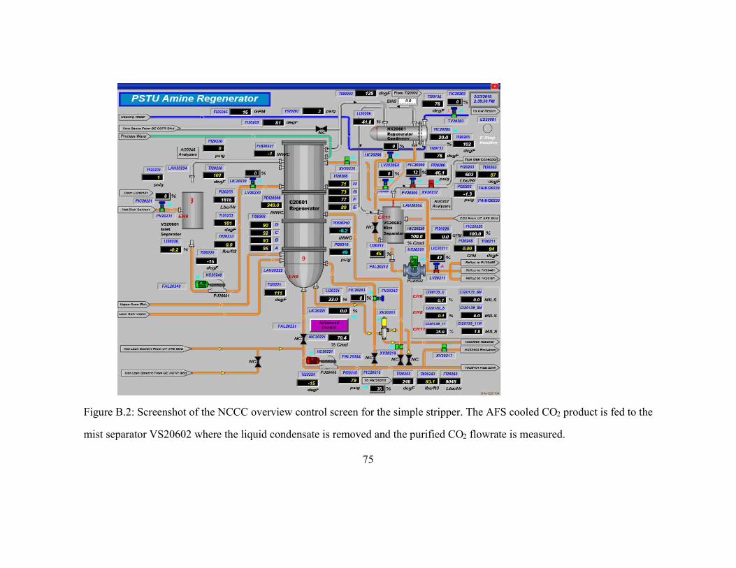
75
Figure B.2: Screenshot of the NCCC overview control screen for the simple stripper. The AFS cooled CO2 product is fed to the
mist separator VS20602 where the liquid condensate is removed and the purified CO2 flowrate is measured.

76
References
Beaudry MR. Aerosol Measurement and Mitigation in CO2 Capture by Amine Scrubbing.
The University of Texas at Austin. Ph.D. Dissertation. 2018.
Bottoms. R. Patent No. 1,783,901. United States of America. December 2, 1930.
Chen E, Fulk SM, Sachde D, Lin YJ, Rochelle GT. “Pilot Plant Activities with
Concentrated Piperazine”. Energy Procedia, 2014;63:1376–1391.
Chen E, Zhang Y, Lin YJ, Nielsen P, Rochelle GT. “Review of Recent Pilot Plant
Activities with Concentrated Piperazine”. Energy Procedia, 2017;114:1110–
1127.
Chen et al. Advanced Flash Stripper with Concentrated Piperazine and Absorber
Intercooling. The University of Texas at Austin. Internal Report. 2017.
EIA. (2018). Annual Energy Outlook 2018 with projections to 2050. Annual Report.
2018.
Fine NA. Nitrosamine Management in Aqueous Amines for Post-Combustion Carbon
Capture. The University of Texas at Austin. Ph.D. Dissertation. 2015.
Frailie PT. Modeling of Carbone Dioxide Absorption/Stripping by Aqueous
Methyldiethanolamine/Piperazine. The University of Texas at Austin. Ph.D.
Dissertation. 2014.
Freeman SA. Thermal Degradation and Oxidation of Aqueous Piperazine for Carbon
Dioxide Capture. The University of Texas at Austin. Ph.D. Dissertation. 2011.

77
Garcia H, Keefer L, Lijinsky W. “Carcinogenicity of Nitrosothiomorpholine and 1-
Nitrosopiperazine in Rats.” Z. Krebsforsch 1970;74: 179– 184.
Hilliard, MD. A Predictive Thermodynamic Model for an Aqueous Blend of Potassium
Carbonate, Piperazine, and Monoethanolamine for Carbon Dioxide Capture from
Flue Gas. The University of Texas at Austin. Ph.D. Dissertation. 2008
Huie RE, Neta P. “Chemical Behavior of Sulfur Trioxide SO3- and SO5
- Radicals in
Aqueous Solutions.” J Phys Chem-US. 1984;88(23):5665–5669.
Lin YJ, Chen E, Rochelle GT. “Pilot plant test of the advanced flash stripper for CO2
capture”. Faraday Discuss. 2016;192, 37–58.
Lin YJ, Rochelle GT. “Optimization of Advanced Flash Stripper for CO2 Capture using
Piperazine”. Energy Procedia 2014;63:1504–1513.
Lin YJ. Modeling Advanced Flash Stripper for Carbon Dioxide Capture Using Aqueous
Amines. The University of Texas at Austin. Ph.D. Dissertation. 2016.
Madan T. Modeling of Stripper Configurations for CO2 Capture using Aqueous
Piperazine. The University of Texas at Austin. M.S. Thesis. 2013.
Nash T. “The Effect of Nitrogen Dioxide and of some Transition Metals on the Oxidation
of Dilute Bisulphite Solutions.” Atmos Environ. 1979;13(8):1149–1154.
Nielsen P. Oxidation of Piperazine in Post-Combustion Carbon Capture. The University
of Texas at Austin. Ph.D. Dissertation. 2017.
Owens DR. Sulfite Oxidation Inhibited by Thiosulfate. The University of Texas at Austin.
M.S. Thesis. 1984.

78
Plaza JM. Modeling of Carbon Dioxide Absorption using Aqueous Monoethanolamine,
Piperazine and Promoted Potassium Carbonate. The University of Texas at
Austin. Ph.D. Dissertation. 2011.
Rochelle GT. “Amine scrubbing for CO2 capture”. Science 2009;325:1652–1654.
Sachde D. Absorber Performance and Configurations for CO2 Capture Using Aqueous
Piperazine. The University of Texas at Austin. Ph.D. Dissertation. 2016.
Sapkota VN, Fine NA, Rochelle GT. “NO2-Catalyzed Sulfite Oxidation.” Ind Eng Chem
Res. 2015;54:4815–4822.
Selinger JL, Rochelle GT. “Analysis of advanced flash stripper performance using 5 m
piperazine.” Proceedings of GHGT-14, Melbourne, Australia. 2018
Sexton A et al. “Minimizing Solvent Oxidation with NO2 Prescrubbing.” Paper #CMTC-
486336-MS. Carbon Management Technology Conference. 2017.
Shen CH. Nitrogen Dioxide Absorption in Aqueous Sodium Sulfite. PhD Dissertation.
The University of Texas at Austin. 1997.
Song D. Effect of Liquid Viscosity on Liquid Film Mass Transfer for Packings. The
University of Texas at Austin. Ph.D. Dissertation. 2017.
Van Wagener DH. Stripper Modeling for CO2 Removal Using Monoethanolamine and
Piperazine Solvents. The University of Texas at Austin. Ph.D. Dissertation. 2011.
Voice, A. K. 2013. Amine Oxidation in Carbon Dioxide Capture by Aqueous Scrubbing.
PhD Dissertation. The University of Texas at Austin.

79
Walters MS. Dynamic Modeling of Post-Combustion Amine Scrubbing for Process
Control Strategy Development. The University of Texas at Austin. Ph.D.
Dissertation. 2016.
Zhang Y, Sachde D, Chen E, Rochelle GT. “Modeling of absorber pilot plant
performance for CO2 capture with aqueous piperazine.” Int. J. Greenh. Gas Con.
2017. 64, 300–313.
Related Documents