Copyright by Gillian Roxanne Grindstaff 2021

Copyright

by

Gillian Roxanne Grindstaff

2021

The Dissertation Committee for Gillian Roxanne Grindstaffcertifies that this is the approved version of the following dissertation:

Geometric Data Analysis for Phylogenetic Trees and

Non-contractible Manifolds

Committee:

Andrew Blumberg, Co-Supervisor

David Ben-Zvi, Co-Supervisor

Lewis Bowen

Megan Owen

Ngoc Tran



by

Gillian Roxanne Grindstaff

DISSERTATION

Presented to the Faculty of the Graduate School of

The University of Texas at Austin

in Partial Fulfillment

of the Requirements

for the Degree of

DOCTOR OF PHILOSOPHY

THE UNIVERSITY OF TEXAS AT AUSTIN

August 2021

Dedicated to my father, Chuck.

Acknowledgments

I would like to thank my committee members for their mentorship,

encouragement, and teaching. In particular, the content of Chapter 3 was

developed in collaboration with Megan Owen, who was extremely patient with

me in the process of writing and submitting my first paper.

I am deeply grateful for the camaraderie and support of all my fellow

grad students at UT, especially my academic siblings, MGMN, and the cohort

of 2015 - you made it joyful, when it didn’t have to be. I’d also like to thank

my real siblings, Russell and Abby, for being stellar roommates. And I could

not have made it without Eliza, Katie, Mike, and Hadrien, who supported me

through countless personal and professional struggles.

Most of all, I owe a profound debt of gratitude to my advisor, Andrew

Blumberg. His unwavering encouragement and enthusiasm for my success

carried me through grad school - I would not have finished this degree without

him.

v



Publication No.

Gillian Roxanne Grindstaff, Ph.D.

The University of Texas at Austin, 2021

Supervisors: Andrew BlumbergDavid Ben-Zvi

A phylogenetic tree is an acyclic graph with distinctly labeled leaves,

whose internal edges have a positive weight. Given a set {1, 2, . . . , n} of n

leaves, the collection of all phylogenetic trees with this leaf set can be as-

sembled into a metric cube complex known as phylogenetic tree space, or

Billera-Holmes-Vogtmann tree space, after [9]. In Chapter 2, we show that

the isometry group of this space is the symmetric group Sn. This fact is rele-

vant to the analysis of some statistical tests of phylogenetic trees, such as those

introduced in [11]. In Chapter 3, co-authored with Megan Owen, we give a

rigorous framework for comparing trees in different moduli spaces of phyloge-

netic trees, and apply this to define extension spaces of trees, a conservative

split-based supertree construction method, and two measures of compatibility

between tree fragments.

In Chapter 4, we discuss some techniques in manifold learning, and

outline a new topologically-constrained nonlinear dimensionality reduction al-

vi

gorithm, which quickly reduces a nerve complex build on local tangent space

approximations to produce a small number of manifold charts, visualized by a

collection of least squares alignments of contractible components. We also give

a method to optimize tangent space alignment on a sphere, and a template

for using local tensor decomposition of higher-order moments to extend this

technique to intersecting and stratified manifolds.

vii

Table of Contents

Acknowledgments v

Abstract vi

List of Figures x

Chapter 1. Phylogenetic tree space 1

1.1 Notation and Definitions . . . . . . . . . . . . . . . . . . . . . 2

1.1.1 Phylogenetic trees . . . . . . . . . . . . . . . . . . . . . 2

1.1.2 Tree Space . . . . . . . . . . . . . . . . . . . . . . . . . 4

1.1.3 Link graph . . . . . . . . . . . . . . . . . . . . . . . . . 6

Chapter 2. Isometries of phylogenetic tree space 7

2.1 Background . . . . . . . . . . . . . . . . . . . . . . . . . . . . 7

2.1.1 Automorphisms versus isometries . . . . . . . . . . . . . 9

2.2 Main Theorem . . . . . . . . . . . . . . . . . . . . . . . . . . . 10

2.2.1 Link Automorphisms . . . . . . . . . . . . . . . . . . . 11

2.2.2 Measure and Isometry . . . . . . . . . . . . . . . . . . . 17

2.2.3 Proof of Main Theorem . . . . . . . . . . . . . . . . . . 20

Chapter 3. Representations of Partial Leaf Sets 23

3.1 Introduction . . . . . . . . . . . . . . . . . . . . . . . . . . . . 24

3.2 Background . . . . . . . . . . . . . . . . . . . . . . . . . . . . 28

3.2.1 Tree dimensionality reduction . . . . . . . . . . . . . . . 29

3.3 The Pre-Image of the Tree Dimensionality Reduction Map . . 32

3.3.1 Extension by one leaf . . . . . . . . . . . . . . . . . . . 34

3.3.2 Extension by Multiple Leaves . . . . . . . . . . . . . . . 38

3.3.3 Calculating the Metric Extension Space . . . . . . . . . 39

3.3.3.1 Combinatorial Step . . . . . . . . . . . . . . . . 40

viii

3.3.3.2 Metric Step . . . . . . . . . . . . . . . . . . . . 46

3.3.4 Comparing extension spaces . . . . . . . . . . . . . . . . 51

3.4 Extension of tree sets . . . . . . . . . . . . . . . . . . . . . . . 53

3.4.1 Combinatorial intersection . . . . . . . . . . . . . . . . 56

3.4.2 Metric intersection . . . . . . . . . . . . . . . . . . . . . 58

3.5 Relaxation . . . . . . . . . . . . . . . . . . . . . . . . . . . . . 61

3.5.1 Uniform α-relaxation . . . . . . . . . . . . . . . . . . . 62

3.5.1.1 Computing αT . . . . . . . . . . . . . . . . . . 67

3.5.1.2 Computing ENT (α) . . . . . . . . . . . . . . . . 69

3.5.2 Proportional relaxation . . . . . . . . . . . . . . . . . . 69

Chapter 4. Manifold Learning and Dimensionality Reductionfor Non-trivial Topology 72

4.1 Introduction . . . . . . . . . . . . . . . . . . . . . . . . . . . . 72

4.2 Gaussian mixture model fitting . . . . . . . . . . . . . . . . . . 76

4.3 Tensor Decomposition . . . . . . . . . . . . . . . . . . . . . . . 79

4.3.1 Data Moments . . . . . . . . . . . . . . . . . . . . . . . 79

4.3.2 GPCA using symmetric block decomposition . . . . . . 80

4.3.3 Local rank estimation . . . . . . . . . . . . . . . . . . . 82

4.4 Multiple charts . . . . . . . . . . . . . . . . . . . . . . . . . . 84

4.4.1 Procedure . . . . . . . . . . . . . . . . . . . . . . . . . . 88

4.4.2 Transition Maps . . . . . . . . . . . . . . . . . . . . . . 91

4.4.3 Intersection Spaces . . . . . . . . . . . . . . . . . . . . . 91

4.4.4 Nerve Conjectures . . . . . . . . . . . . . . . . . . . . . 92

4.5 The alignment G . . . . . . . . . . . . . . . . . . . . . . . . . 93

4.5.1 Flat alignment of Gaussians . . . . . . . . . . . . . . . . 93

4.5.2 Example . . . . . . . . . . . . . . . . . . . . . . . . . . 99

4.5.3 Spherical Alignment . . . . . . . . . . . . . . . . . . . . 100

Index 102

Bibliography 103

Vita 112

ix

List of Figures

1.1 Phylogenetic Tree of Life. Image credit Wikimedia Commons. 2

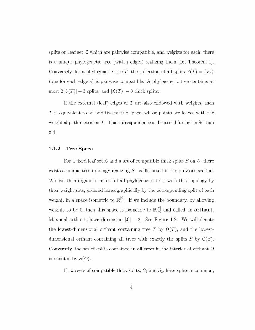
1.2 Left, a single orthant. Center, five orthants identified alongcommon split sets. Right, the link L5 of the origin, isomorphicto the Petersen graph. Image credit [9] and Wikimedia commons. 5

2.2 Left, a neighborhood in BHV5 with volume (3/2)πϵ2; Right, aneighborhood of c, with volume 15/4πϵ2. . . . . . . . . . . . . 21

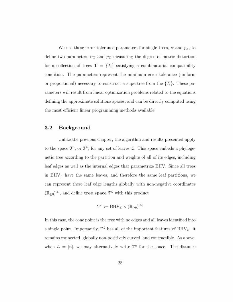
3.1 Left, a tree with 5 leaves. Center, the tree with leaf 5 and itsedge deleted, resulting in a degree two vertex (in red). Right,the tree after concatenating the two edges adjacent to the degreetwo vertex. . . . . . . . . . . . . . . . . . . . . . . . . . . . . . 31

3.2 Left, a tree T with 4 leaves, {1, 2, 3, 5}. Right, the orthantsof T5 containing the preimage Ψ−1

4(T ), with the subspace corre-

sponding to the preimage shown with the thick solid lines. Notethat the dimensions corresponding to the 4 leaf edges lengthswere not included for clarity. . . . . . . . . . . . . . . . . . . . 38

3.3 The connection graph G5T for tree T from Example 3.3.2. The

vertices corresponding to elements ofQ are labeled by the smallerof the two pieces of the partition. The leaf partitions have auto-matic compatibility - these edges are shown dotted, while com-patible thick partitions have colored edges. . . . . . . . . . . 42

3.4 The connection space S5T for tree T from Example 3.3.2. . . . 42

3.5 Left, tree T (repeated from Figure 3.2) and a second tree T ′ withleaves {1, 2, 3, 4}. Center, the T -shaped subspace of Ψ−1

5(T ) and

the T ′-shaped subspace of Ψ−15(T ′), with their unique intersec-

tion circled. Right, the tree at the intersection point of the twosubspaces. . . . . . . . . . . . . . . . . . . . . . . . . . . . . 54

3.6 The extension spaces ENT and EN

T ′′ from Example 3.5.1 inter-sected with the orthant corresponding to splits 13|245, 25|134,and 2|1345. Note that if the extension spaces are projectedonto the 2-dimensional orthant corresponding to splits 13|245and 25|134 they appear to intersect. . . . . . . . . . . . . . . . 63

x

3.7 The α-extension region of tree T from Example 3.3.2 is thedarker shaded region within the 5 orthants. Here α = 0.05. . 65

4.1 Array reference . . . . . . . . . . . . . . . . . . . . . . . . . . 97

4.2 Left, 1000 points on a sphere in R3. Right, the visualized charts. 100

xi

Chapter 1

Phylogenetic tree space

In the context of evolutionary biology, given a set of organisms referred

to as taxa, a phylogenetic tree is a semi-labeled, weighted acyclic graph repre-

senting a possible evolutionary relationship between the taxa, using genotypic

or phenotypic data. Such trees typically have a root which represents the com-

mon ancestor of the taxa, with a branch point at each speciation event, and a

leaf for each taxon, such that the taxa which share more features are “nearer”

to each other in the tree. The phylogenetic tree itself represents a finite metric

space, with metric given by shortest weighted path length: a sequence of edges

without repetition gives a unique path from one leaf to another, and the sum

of their lengths is the distance, quantifying the genetic or phenotypic changes

and differences between the taxa.

In addition to the distances between the taxa that a single phylogenetic

tree represents, a distance between distinct phylogenetic trees with the same

set of taxa can also be defined through the construction of phylogenetic tree

space Tn and BHVn, for taxa labels {1, . . . , n}[9]. Each tree is represented by

a point in tree space, with location determined by the topology (shape) of the

tree and its vector of edge lengths. The BHV distance between two trees is

1

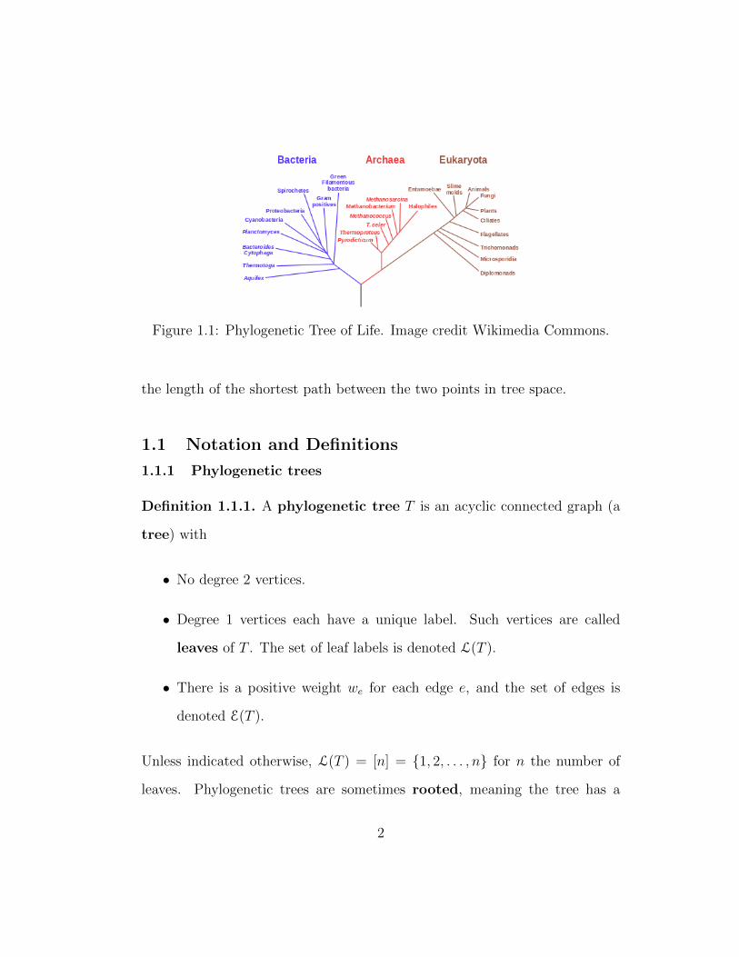
Figure 1.1: Phylogenetic Tree of Life. Image credit Wikimedia Commons.

the length of the shortest path between the two points in tree space.

1.1 Notation and Definitions

1.1.1 Phylogenetic trees

Definition 1.1.1. A phylogenetic tree T is an acyclic connected graph (a

tree) with

• No degree 2 vertices.

• Degree 1 vertices each have a unique label. Such vertices are called

leaves of T . The set of leaf labels is denoted L(T ).

• There is a positive weight we for each edge e, and the set of edges is

denoted E(T ).

Unless indicated otherwise, L(T ) = [n] = {1, 2, . . . , n} for n the number of

leaves. Phylogenetic trees are sometimes rooted, meaning the tree has a

2

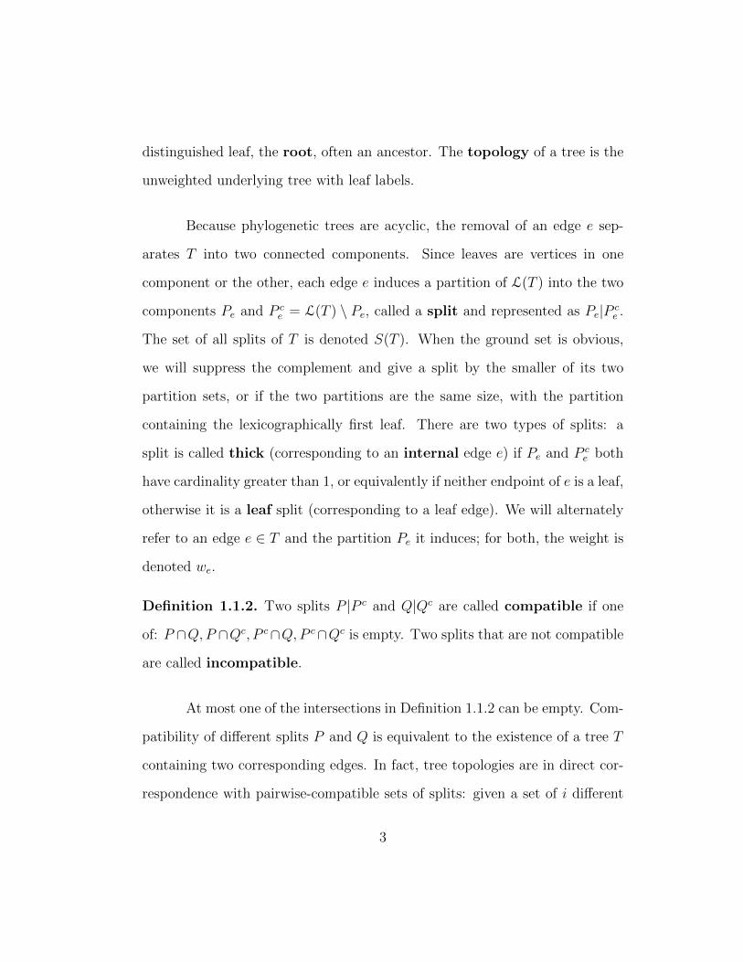
distinguished leaf, the root, often an ancestor. The topology of a tree is the

unweighted underlying tree with leaf labels.

Because phylogenetic trees are acyclic, the removal of an edge e sep-

arates T into two connected components. Since leaves are vertices in one

component or the other, each edge e induces a partition of L(T ) into the two

components Pe and P ce = L(T ) \ Pe, called a split and represented as Pe|P c

e .

The set of all splits of T is denoted S(T ). When the ground set is obvious,

we will suppress the complement and give a split by the smaller of its two

partition sets, or if the two partitions are the same size, with the partition

containing the lexicographically first leaf. There are two types of splits: a

split is called thick (corresponding to an internal edge e) if Pe and P ce both

have cardinality greater than 1, or equivalently if neither endpoint of e is a leaf,

otherwise it is a leaf split (corresponding to a leaf edge). We will alternately

refer to an edge e ∈ T and the partition Pe it induces; for both, the weight is

denoted we.

Definition 1.1.2. Two splits P |P c and Q|Qc are called compatible if one

of: P ∩Q,P ∩Qc, P c∩Q,P c∩Qc is empty. Two splits that are not compatible

are called incompatible.

At most one of the intersections in Definition 1.1.2 can be empty. Com-

patibility of different splits P and Q is equivalent to the existence of a tree T

containing two corresponding edges. In fact, tree topologies are in direct cor-

respondence with pairwise-compatible sets of splits: given a set of i different

3

splits on leaf set L which are pairwise compatible, and weights for each, there

is a unique phylogenetic tree (with i edges) realizing them [16, Theorem 1].

Conversely, for a phylogenetic tree T , the collection of all splits S(T ) = {Pe}

(one for each edge e) is pairwise compatible. A phylogenetic tree contains at

most 2|L(T )| − 3 splits, and |L(T )| − 3 thick splits.

If the external (leaf) edges of T are also endowed with weights, then

T is equivalent to an additive metric space, whose points are leaves with the

weighted path metric on T . This correspondence is discussed further in Section

2.4.

1.1.2 Tree Space

For a fixed leaf set L and a set of compatible thick splits S on L, there

exists a unique tree topology realizing S, as discussed in the previous section.

We can then organize the set of all phylogenetic trees with this topology by

their weight sets, ordered lexicographically by the corresponding split of each

weight, in a space isometric to R|S|+ . If we include the boundary, by allowing

weights to be 0, then this space is isometric to R|S|≥0 and called an orthant.

Maximal orthants have dimension |L| − 3. See Figure 1.2. We will denote

the lowest-dimensional orthant containing tree T by O(T ), and the lowest-

dimensional orthant containing all trees with exactly the splits S by O(S).

Conversely, the set of splits contained in all trees in the interior of orthant O

is denoted by S(O).

If two sets of compatible thick splits, S1 and S2, have splits in common,

4

Figure 1.2: Left, a single orthant. Center, five orthants identified along com-mon split sets. Right, the link L5 of the origin, isomorphic to the Petersengraph. Image credit [9] and Wikimedia commons.

C = S1 ∩ S2, then the orthants corresponding to S1 and S2 each have a

boundary orthant R|C|≥0 that contains the same trees. We identify all such

common boundary orthants to produce a single space, called the Billera-

Holmes-Vogtmann (BHV) treespace and denoted BHVL, where L is the

leaf set of all trees. When L = [n], we will alternatively write BHVn for the

space. The empty split set S = ∅ produces a single point, called the cone

point, 0, which represents the unique star-shaped tree with no internal edges.

The cone point is contained in each orthant at the origin, so the identified space

is path-connected. We define the distance dBHV(T, T′) between points T and

T ′ in this space to be the infimum of the lengths of all piecewise smooth paths

from T to T ′, where path length is calculated by summing the L2 distances of

the path restricted to each orthant it passes through.

The BHV treespace was first proposed by Billera, Holmes, and Vogt-

mann in [9], where they showed that it is a contractible, complete, and globally

non-positively curved, or CAT(0), cube complex. Global non-positive curva-

5

ture implies that there is a unique shortest path, or geodesic, between each pair

of trees in the space. There exists a polynomial time algorithm to calculate

this path and its length, given by Owen and Provan in [45].

1.1.3 Link graph

Definition 1.1.3. The link LL := LL(0) of the cone point 0 is the set of all

trees in BHVL which have internal edge lengths summing to 1. Homeomor-

phically, LL is the set of trees in BHVL at fixed L1 distance from 0.

Because BHVL is a cube complex, LL is a simplicial complex; the face

maps are restrictions of face maps of the cube complex, and every k-face of

the cube complex intersects the link in a (k− 1)-simplex. In particular, the 0-

simplices correspond to single splits, the 1-simplices correspond to compatible

split pairs, and k-simplices correspond to trees sharing the same k non-zero

splits which have edge lengths summing to 1.

6

Chapter 2

Isometries of phylogenetic tree space

BHV space, with geodesic metric, can be used to give precise geometric

characterizations of collections of phylogenies, and to perform various statis-

tical tests, such as those defined in [31], [59], and [5]. In [11], the matrix of

pairwise distances between trees in a set is used as a signature to perform

statistical inference. With techniques like this, which operate on the distance

matrix instead of the trees themselves, the results are insensitive to isometry;

this renders the classification of isometries of BHVn extremely relevant.

In Theorem 2.2.1, previously published in [27], we show that the group

of isometries of BHV space is the symmetric group Sn, for n the total number

of leaves including root. These isometries correspond to simple permutations

of the leaves.

2.1 Background

An orthant boundary component of codimension k corresponds to a

“degenerate” tree topology: trees on the boundary are 0 along k axes, so

k of the edges in the orthant tree topology have length zero. This leaves a

non-binary tree topology with n − k − 3 non-trivial internal edges, and this

7

6

1 2 3 4 5

0.25

0.3

0.45

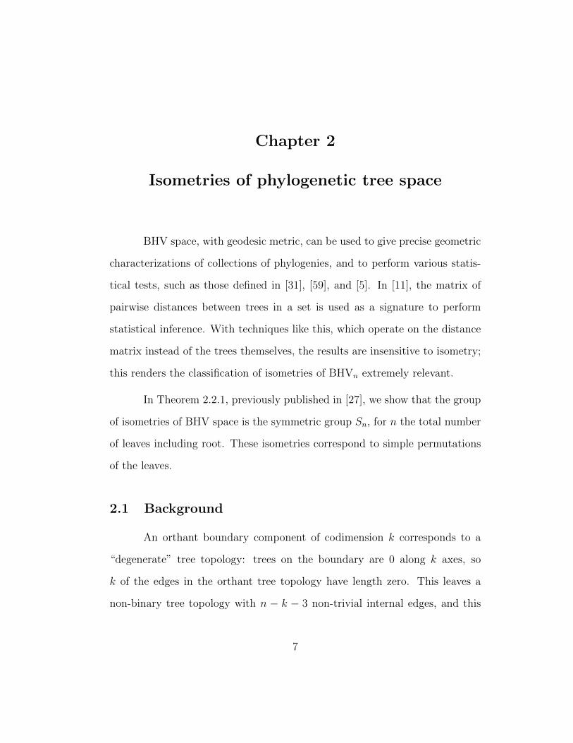
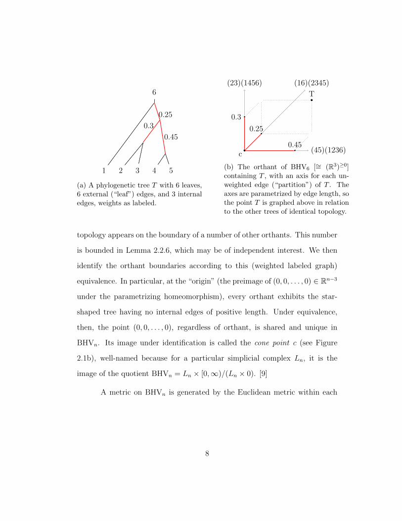
(a) A phylogenetic tree T with 6 leaves,6 external (“leaf”) edges, and 3 internaledges, weights as labeled.

(16)(2345)

c

0.3

0.45

0.25

T

(23)(1456)

(45)(1236)

(b) The orthant of BHV6 [∼= (R3)≥0]containing T , with an axis for each un-weighted edge (“partition”) of T . Theaxes are parametrized by edge length, sothe point T is graphed above in relationto the other trees of identical topology.

topology appears on the boundary of a number of other orthants. This number

is bounded in Lemma 2.2.6, which may be of independent interest. We then

identify the orthant boundaries according to this (weighted labeled graph)

equivalence. In particular, at the “origin” (the preimage of (0, 0, . . . , 0) ∈ Rn−3

under the parametrizing homeomorphism), every orthant exhibits the star-

shaped tree having no internal edges of positive length. Under equivalence,

then, the point (0, 0, . . . , 0), regardless of orthant, is shared and unique in

BHVn. Its image under identification is called the cone point c (see Figure

2.1b), well-named because for a particular simplicial complex Ln, it is the

image of the quotient BHVn = Ln × [0,∞)/(Ln × 0). [9]

A metric on BHVn is generated by the Euclidean metric within each

8

orthant: a path γ between trees T and T ′ has length

ℓ(γ) =∑S∈O

|γ ∩ S|,

where | · | is Euclidean path length via restriction to an orthant, and O is the

set of all orthants in BHVn. Then

d(T, T ′) := infγ:γ(0)=T,γ(1)=T ′

ℓ(γ)

is a complete metric, which is realized by a unique geodesic γ with ℓ(γ) =

d(T, T ′) [9]. The natural Lebesgue measure for open sets in BHV is described

analogously in Section 2.2.2 in order to give the volume of small neighborhoods

of points in BHVn; we suspect this might also be of independent interest.

2.1.1 Automorphisms versus isometries

It might seem natural to classify isometries of BHVn, which is a CAT(0)

cube complex (see [48]), via natural isomorphisms of that structure. However,

it is important to note that in general, isometries of cube complexes can ex-

ceed their cube complex automorphisms, and if the cubes are endowed with a

different metric, an automorphism may not be an isometry at all. As a trivial

example, one can consider the integer cubulation of R2, which in addition to

the D4 × Z2 lattice isometries, retains the O(2) × R2 real isometries, which

do not preserve the cube complex structure. This discrepancy was addressed

recently in [14] - Bregman shows that for a CAT(0) cube complex C with unit

euclidean metric on each cube and global metric given by minimal path length,

9

if Isom(C) = Aut(C), then there is a full subcomplex D of C admitting a de-

composition into a product E ×Rn , where E is a full subcomplex of D. This

shows that in some sense, the only additional isometries come from an Rn-type

subcomplex, possibly with non-flat curvature. We note that our result gives

a counterexample to the converse: the full subcomplex of BHV5 given by any

5-cycle in the link is R2 with the singular cone metric Cone(R2, 5), but we do

not gain any additional isometries.

Besides the proof given in Section 2.2.1 of this chapter, Aut(BHVn) is

known from the work of Abreu and Pacini classifying cone complex automor-

phisms of the moduli space M trop0,n of tropical genus 0 curves with n marked

points[1]. Their result is closely related to our Proposition 2.2.3. Inspection

of the argument suggests that they are proving the same essential combina-

torial fact, through an inductive technique. In fact, our main result could be

proved via theirs through a direct application of Lemma 2.2.6 to the interior

of top-dimensional orthants, analogously to our proof in Section 2.2.3 that

Aut(Ln) = Isom(Ln).

2.2 Main Theorem

Theorem 2.2.1. For n ≥ 3, the isometry group of BHVn is isomorphic to

Sn. These isometries correspond to permutation of leaf labels.

It is clear that a permutation of the leaf labels induces an isometry

from BHVn to itself, so the following lemmas will build to the converse. This

10

will involve two stages.

First, in Section 2.2.1 we will use the Erdos-Ko-Rado theorem to give a

new proof that the automorphism group of Ln, the spherical simplicial complex

of points at distance 1 from the origin, is Sn. As we’ve remarked already, this

fact is implied by recent work of [1], who computed the automorphisms of

BHVn as a cone complex.

In Section 2.2.2, we will then give local bounds on the natural volume

measure in BHVn to show that any isometry of BHVn induces a self-map of the

unit sphere Ln, and any isometry of the unit sphere to itself is an automorphism

of simplicial complexes. Having classified these in the previous section, we

conclude in Section 2.2.3 that any isometric automorphism of BHVn must be

a relabeling.

2.2.1 Link Automorphisms

Following [9], BHVn can be expressed as a cone on a simplicial complex

Ln, constructed:

• A 0-simplex (vertex) v for each subset Pv ⊂ {1, 2, . . . , n} such that 2 ≤

|Pv| < n/2. The size |Pv| will often be denoted k. Each Pv determines a

partition Pv, Pcv of [n], unique for k < n/2. If n is even, we also include

a vertex for each pair P, P c with |P | = |P c| = n/2.

• A 1-simplex (edge) (v, w) for each compatible pair (Pv, Pcv ) and (Pw, P

cw).

Pv and Pw are said to be compatible if one of the sets [Pv ∩ Pw, Pv ∩

11

P cw, P

cv ∩Pw, P

cv ∩P c

w] is empty. We will simplify this condition in Lemma

2.2.2.

• The complex (graph) constructed up to this point is denoted L1n, the

1-skeleton of Ln.

• Ln is the simplicial complex with a k-simplex, k > 1, for each (k + 1)-

clique present in L1n (i.e. Ln is a flag simplicial complex).

• Ln is realized geometrically as a right-angled spherical simplicial com-

plex: for Sk the unit sphere in Rk, each simplex is isometric to

{(x1, . . . , xk+1) ∈ Sk : xi ≥ 0 for all i}

with the spherical metric.

• Finally, BHVn is a right-angled spherical metric cone on Ln, as described

in [17]. Practically, this means that each tree topology is parametrized

by n − 3 non-negative, real coordinates, with the local standard metric

in Rn−3, as shown in the introduction.

We begin with some facts about L1n, and then show the automorphism group

of L1n in Proposition 2.2.3. This gives the automorphisms of Ln via the flag

property in Corollary 2.2.4.

Lemma 2.2.1. The degree of a vertex v of partition size k in L1n is given by:

deg(v) = 2k + 2n−k − n− 4

12

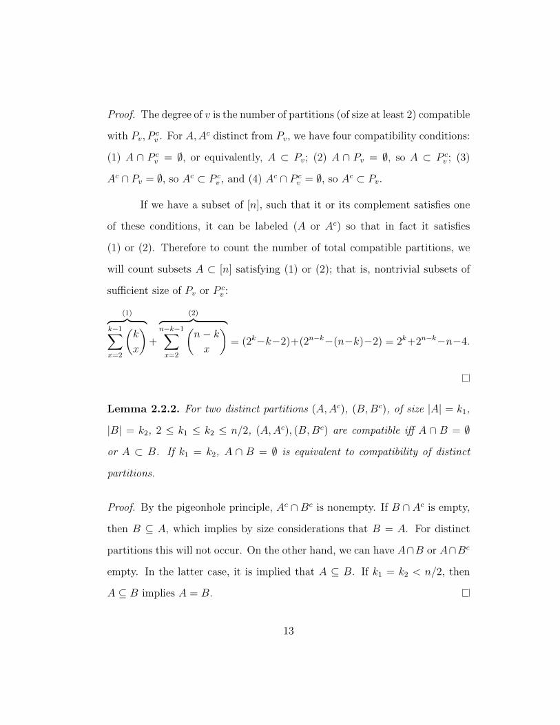
Proof. The degree of v is the number of partitions (of size at least 2) compatible

with Pv, Pcv . For A,A

c distinct from Pv, we have four compatibility conditions:

(1) A ∩ P cv = ∅, or equivalently, A ⊂ Pv; (2) A ∩ Pv = ∅, so A ⊂ P c

v ; (3)

Ac ∩ Pv = ∅, so Ac ⊂ P cv , and (4) Ac ∩ P c

v = ∅, so Ac ⊂ Pv.

If we have a subset of [n], such that it or its complement satisfies one

of these conditions, it can be labeled (A or Ac) so that in fact it satisfies

(1) or (2). Therefore to count the number of total compatible partitions, we

will count subsets A ⊂ [n] satisfying (1) or (2); that is, nontrivial subsets of

sufficient size of Pv or P cv :

(1)︷︸︸︷k−1∑x=2

(k

x

)+

(2)︷︸︸︷n−k−1∑x=2

(n− k

x

)= (2k−k−2)+(2n−k−(n−k)−2) = 2k+2n−k−n−4.

Lemma 2.2.2. For two distinct partitions (A,Ac), (B,Bc), of size |A| = k1,

|B| = k2, 2 ≤ k1 ≤ k2 ≤ n/2, (A,Ac), (B,Bc) are compatible iff A ∩ B = ∅

or A ⊂ B. If k1 = k2, A ∩ B = ∅ is equivalent to compatibility of distinct

partitions.

Proof. By the pigeonhole principle, Ac ∩ Bc is nonempty. If B ∩ Ac is empty,

then B ⊆ A, which implies by size considerations that B = A. For distinct

partitions this will not occur. On the other hand, we can have A∩B or A∩Bc

empty. In the latter case, it is implied that A ⊆ B. If k1 = k2 < n/2, then

A ⊆ B implies A = B.

13

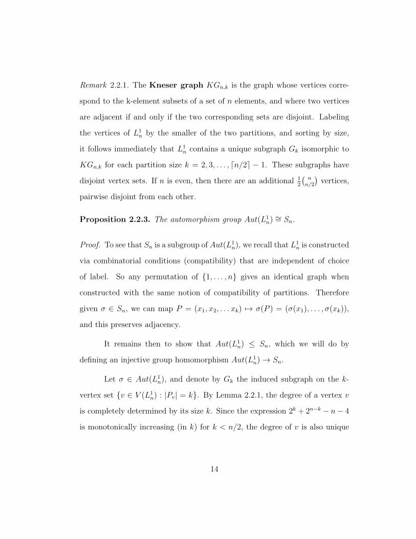
Remark 2.2.1. The Kneser graph KGn,k is the graph whose vertices corre-

spond to the k-element subsets of a set of n elements, and where two vertices

are adjacent if and only if the two corresponding sets are disjoint. Labeling

the vertices of L1n by the smaller of the two partitions, and sorting by size,

it follows immediately that L1n contains a unique subgraph Gk isomorphic to

KGn,k for each partition size k = 2, 3, . . . , ⌈n/2⌉ − 1. These subgraphs have

disjoint vertex sets. If n is even, then there are an additional 12

(n

n/2

)vertices,

pairwise disjoint from each other.

Proposition 2.2.3. The automorphism group Aut(L1n)

∼= Sn.

Proof. To see that Sn is a subgroup of Aut(L1n), we recall that L

1n is constructed

via combinatorial conditions (compatibility) that are independent of choice

of label. So any permutation of {1, . . . , n} gives an identical graph when

constructed with the same notion of compatibility of partitions. Therefore

given σ ∈ Sn, we can map P = (x1, x2, . . . xk) 7→ σ(P ) = (σ(x1), . . . , σ(xk)),

and this preserves adjacency.

It remains then to show that Aut(L1n) ≤ Sn, which we will do by

defining an injective group homomorphism Aut(L1n) → Sn.

Let σ ∈ Aut(L1n), and denote by Gk the induced subgraph on the k-

vertex set {v ∈ V (L1n) : |Pv| = k}. By Lemma 2.2.1, the degree of a vertex v

is completely determined by its size k. Since the expression 2k + 2n−k − n− 4

is monotonically increasing (in k) for k < n/2, the degree of v is also unique

14

to vertices of the same partition size. This means that σ(v) must be contained

in Gk, so σ restricts to a graph automorphism on Gk.

We now show that this restriction map Aut(L1n) → Aut(Gk) is injective

for 2 ≤ k < n/2. Let σidk be an automorphism of L1n which acts as the identity

on Gk. Then we show that Gk+1 is fixed as well, using the fact that adjacencies

to Gk are preserved under automorphism.

Let N(Pv)+1 denote the set of neighbors of v ∈ Gk ⊂ L1

n of size k + 1,

i.e.

N(Pv)+1 = {Pw ∈ Gk+1 : Pv ⊂ Pw or Pv ∩ Pw = ∅}

by Lemma 2.2.2. Similarly, we denote byN(Pv)−1 the set of neighbors of v with

partitions one size lower: N(Pv)−1 = {Pw ∈ Gk−1 : Pw ⊂ Pv or Pv ∩ Pw = ∅}.

Let Pz = (x1, x2, . . . , xk+1) ∈ Gk+1. Then (x1, x2, . . . , xk+1) is the unique

partition of size k + 1 which is compatible with all of its size-k neighbors:

{Pz} =⋂

Pv∈N(Pz)−1

N(Pv)+1

To show this, we note that for two distinct (k + 1)-partitions of the same

size, there exists at least one set of k labels which is compatible with one and

not the other: for Pw = Pz, there is a label i ∈ Pw, i /∈ Pz and there is a

j ∈ P cw, j /∈ Pz (by size considerations), so that any k-subset of P c

z containing

both i and j is compatible with Pz, but cannot be compatible with Pw, which

excludes Pw from this intersection.

15

Now, since adjacencies and Gk are preserved by any automorphism,

N(Pv)+1 is preserved by σidk for v ∈ Gk. So we can conclude by the set

equivalence above that Pz is preserved as well, which gives the desired result

that σidk(Gk+1) = Gk+1, which implies that Gj for j > k is preserved under σ,

by repetition of the same argument. We have

Pz =⋂

α∈P cz

N(x1 . . . xk, α)−1,

which shows σidk(Gj) = Gj for j < k in the same manner. Since V (L1n) =⊔⌊n/2⌋

k=1 V (Gk), we have shown that σidk ∈ ker(Aut(L1n) → Aut(Gk)) acts triv-

ially on the vertices of L1n, so must be the trivial automorphism.

Now following [24], we show that Aut(Gk) ∼= Sn for 2 ≤ k < n/2. By

the Erdos-Ko-Rado Theorem, any family of subsets of {1, 2, . . . , n} of uniform

size k having pairwise-nonempty intersection has size ≤(n−1k−1

), and the subsets

achieving equality are of the form

G(i)k = {v ∈ Gk : i ∈ Pv}

for i ∈ [n].[22] Since these partitions pairwise-intersect, they are pairwise

disjoint in Gk, and by definition form a maximum-size independent set in

Gk. Correspondingly, σ ∈ Aut(Gk) must induce a permutation on these

maximum independent sets, which determines a (surjective) homomorphism

Aut(Gk) → Sn. To see that this is an isomorphism, note that if σ fixes the

G(i)k , it must be the identity: suppose σ(v) = v. Then there exists some j ∈ Pv

such that j /∈ Pσ(v). This would imply that σ(G(j)k ) = G

(j)k , a contradiction.

16

Now we see that Aut(L1n)

∼= Aut(Gk) ∼= Sn (for any/all 2 ≤ k < n/2,

we really only needed one), which completes the proof.

Corollary 2.2.4. The group of simplicial automorphisms of Ln is isomorphic

to Aut(L1n).

Proof. Let n ≥ 3 be given. First we note that Aut(Ln) = Aut(L1n): each sim-

plicial automorphism induces an automorphism of the 1-skeleton, and since

Ln contains no simplices with the same 1-skeleton, this map is injective. Then

since Ln is a flag complex ([9]), given a graph automorphism of L1n, we can de-

fine a canonical extension by sending a k-simplex to the k-simplex determined

by the image of its 1-skeleton k-clique.

2.2.2 Measure and Isometry

We will now consider the entire metric space BHVn, and show that the

standard embedding of Ln into the unit sphere is invariant under isometry.

There is a natural volume measure µ on B(BHVn), which is given by

the local Lebesgue measure in each orthant. Explicitly, for A ∈ B(BHVn),

µ(A) =∑S

|A ∩ S|

where S ∼= (R+)n−3 is an orthant of BHVn and |·| is the real Lebesgue measure.

As we will see in the following lemmas, the volume of small neighborhoods can

vary exponentially under translation; this fact is one of the major impediments

to statistical techniques in tree space.

17

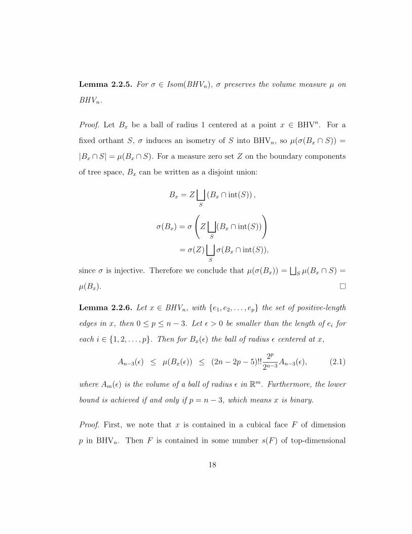
Lemma 2.2.5. For σ ∈ Isom(BHVn), σ preserves the volume measure µ on

BHVn.

Proof. Let Bx be a ball of radius 1 centered at a point x ∈ BHVn. For a

fixed orthant S, σ induces an isometry of S into BHVn, so µ(σ(Bx ∩ S)) =

|Bx ∩ S| = µ(Bx ∩ S). For a measure zero set Z on the boundary components

of tree space, Bx can be written as a disjoint union:

Bx = Z⊔S

(Bx ∩ int(S)) ,

σ(Bx) = σ

(Z⊔S

(Bx ∩ int(S))

)= σ(Z)

⊔S

σ(Bx ∩ int(S)),

since σ is injective. Therefore we conclude that µ(σ(Bx)) =⊔

S µ(Bx ∩ S) =

µ(Bx).

Lemma 2.2.6. Let x ∈ BHVn, with {e1, e2, . . . , ep} the set of positive-length

edges in x, then 0 ≤ p ≤ n− 3. Let ϵ > 0 be smaller than the length of ei for

each i ∈ {1, 2, . . . , p}. Then for Bx(ϵ) the ball of radius ϵ centered at x,

An−3(ϵ) ≤ µ(Bx(ϵ)) ≤ (2n− 2p− 5)!!2p

2n−3An−3(ϵ), (2.1)

where Am(ϵ) is the volume of a ball of radius ϵ in Rm. Furthermore, the lower

bound is achieved if and only if p = n− 3, which means x is binary.

Proof. First, we note that x is contained in a cubical face F of dimension

p in BHVn. Then F is contained in some number s(F ) of top-dimensional

18

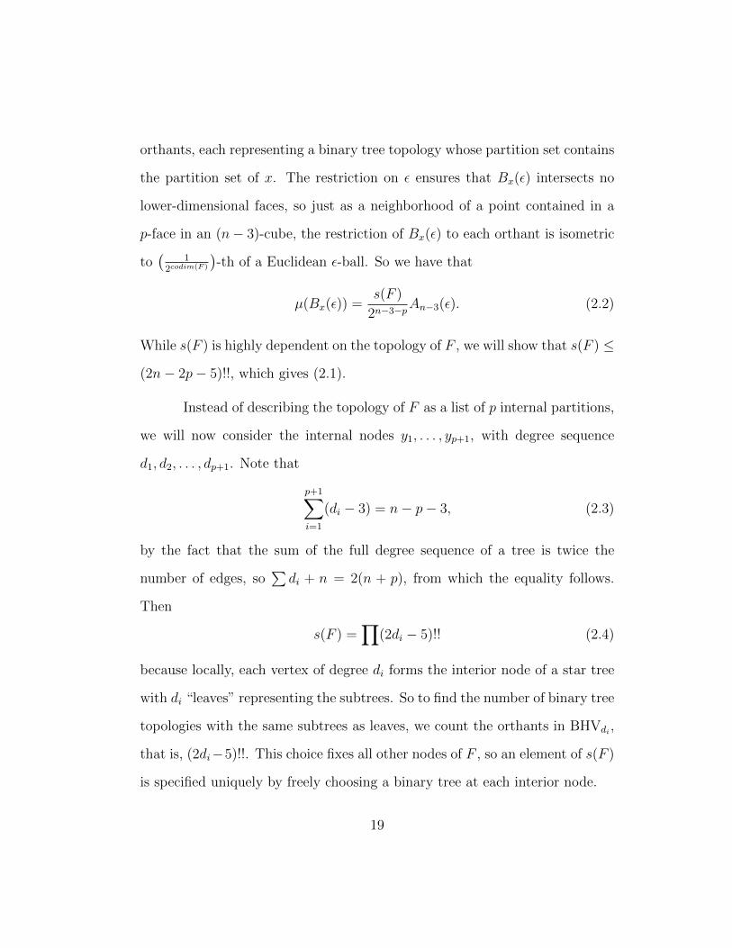
orthants, each representing a binary tree topology whose partition set contains

the partition set of x. The restriction on ϵ ensures that Bx(ϵ) intersects no

lower-dimensional faces, so just as a neighborhood of a point contained in a

p-face in an (n− 3)-cube, the restriction of Bx(ϵ) to each orthant is isometric

to(

12codim(F )

)-th of a Euclidean ϵ-ball. So we have that

µ(Bx(ϵ)) =s(F )

2n−3−pAn−3(ϵ). (2.2)

While s(F ) is highly dependent on the topology of F , we will show that s(F ) ≤

(2n− 2p− 5)!!, which gives (2.1).

Instead of describing the topology of F as a list of p internal partitions,

we will now consider the internal nodes y1, . . . , yp+1, with degree sequence

d1, d2, . . . , dp+1. Note that

p+1∑i=1

(di − 3) = n− p− 3, (2.3)

by the fact that the sum of the full degree sequence of a tree is twice the

number of edges, so∑

di + n = 2(n + p), from which the equality follows.

Then

s(F ) =∏

(2di − 5)!! (2.4)

because locally, each vertex of degree di forms the interior node of a star tree

with di “leaves” representing the subtrees. So to find the number of binary tree

topologies with the same subtrees as leaves, we count the orthants in BHVdi ,

that is, (2di−5)!!. This choice fixes all other nodes of F , so an element of s(F )

is specified uniquely by freely choosing a binary tree at each interior node.

19

Next we note that (2di − 5)!! has di − 3 terms greater than 1. For

any degree sequence di, we then have by (2.3) that the product (2.4) has

(n− p− 3) non-trivial terms, each of which is at least 3, which gives the lower

bound. This product is maximized with the degree sequence n− p, 3, 3, . . . , 3,

for which s(F ) = (2(n−p)−5)!!, which gives the upper bound. For p < n−3,

s(F ) is strictly greater than 2n−3−p. For p = n − 3, we have a coefficient of

1. These two facts show that the lower bound is achieved only for binary

trees.

Corollary 2.2.7. Let n ≥ 4, c the cone point in BHVn, x = c ∈ BHVn. Then

µ(Bc(ϵ)) > µ(Bx(ϵ)) for ϵ < mine∈E(x) we, where E(x) is the set of edges of x

as a graph, and we their respective weight in x, so that ϵ is smaller than the

length of the smallest non-zero edge of x.

Proof. First note that µ(Bc(ϵ)) =(2n−5)!!2n−3 An−3(ϵ) for any ϵ > 0, where Am(ϵ)

is the volume of a ball of radius ϵ in Rm. Then for x = c, p ≥ 1, so by Lemma

2.2.6,

µ(Bx(ϵ)) ≤ (2n− 7)!!2

2n−3An−3(ϵ).

But since 2 < 2n− 5, µ(Bx(ϵ)) < µ(Bc(ϵ)).

2.2.3 Proof of Main Theorem

Proof. Let n ≥ 4 be given.

Each of the relabeling automorphisms of Ln is an isometry, and it ex-

tends in the obvious way to an isometry of BHVn by relabeling the leaves of

20

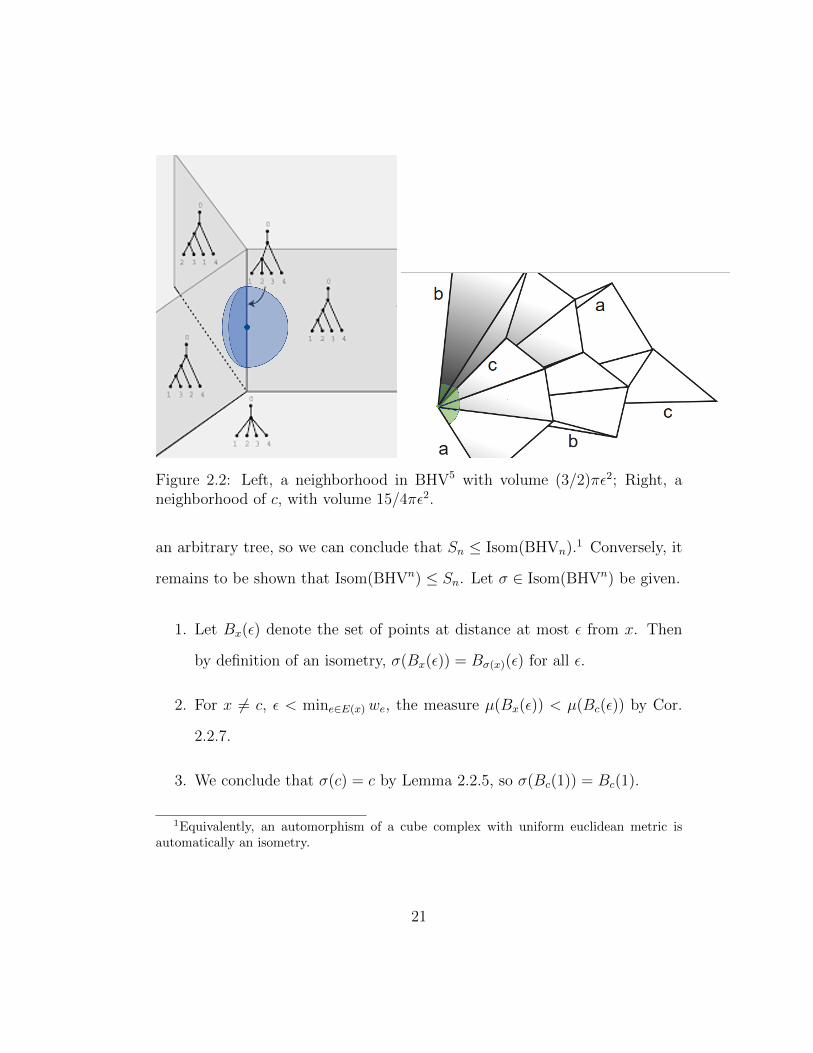
Figure 2.2: Left, a neighborhood in BHV5 with volume (3/2)πϵ2; Right, aneighborhood of c, with volume 15/4πϵ2.

an arbitrary tree, so we can conclude that Sn ≤ Isom(BHVn).1 Conversely, it

remains to be shown that Isom(BHVn) ≤ Sn. Let σ ∈ Isom(BHVn) be given.

1. Let Bx(ϵ) denote the set of points at distance at most ϵ from x. Then

by definition of an isometry, σ(Bx(ϵ)) = Bσ(x)(ϵ) for all ϵ.

2. For x = c, ϵ < mine∈E(x) we, the measure µ(Bx(ϵ)) < µ(Bc(ϵ)) by Cor.

2.2.7.

3. We conclude that σ(c) = c by Lemma 2.2.5, so σ(Bc(1)) = Bc(1).

1Equivalently, an automorphism of a cube complex with uniform euclidean metric isautomatically an isometry.

21

4. Since Ln = ∂(Bc(1)) is the set of points at distance 1 from c, we conclude

that σ(Ln) = Ln.

5. In the remainder of the proof, we will show that Isom(Ln) = Aut(Ln) ∼=

Sn, and this will give the titular result.

Let σ ∈ Isom(Ln)be given. Let x ∈ Ln be a binary tree, so x is contained in

the interior of an (n−4)-simplex. Then by Lemma 2.2.6 and Lemma 2.2.5, σ(x)

is also necessarily a binary tree, and so contained in the interior of an (n− 4)-

simplex in Ln. An isometry which restricts to τ : int(∆n−4) → int(∆n−4) on

the interior of an (n − 4)-simplex must extend by continuity to an isometry

τ : ∆n−4 → ∆n−4. Such an isometry is a simplicial map, sending k-simplices

to k-simplices. But every k-simplex in Ln is on the boundary of a maximal

simplex (equivalently, every non-binary tree has a choice of additional edges

making it binary), so we conclude that σ is a simplicial map from Ln to Ln,

i.e. σ ∈ Aut(Ln). Since every automorphism is an isometry, we conclude

Isom(Ln) ∼= Aut(Ln), and by Corollary 2.2.4, Aut(L1n)

∼= Aut(Ln) ∼= Sn.

22

Chapter 3

Representations of Partial Leaf Sets

Phylogenetric tree space allows for direct comparison and summary of

trees that have different shape and size. However, it is sometimes necessary to

analyze collections of trees on nonidentical taxa sets (i.e., with different num-

bers of leaves), and in this context it is not evident how to apply BHV space.

Ren et al. [46] approach this problem by describing a combinatorial algorithm

extending tree topologies to regions in higher-dimensional tree spaces, so that

one can quickly compute which topologies contain a given tree as partial data.

In this work, joint with Megan Owen, and previously published in [28], we

refine and adapt their algorithm to work for metric trees to give a full char-

acterization of the subspace of extensions of a subtree (see Algorithm 1 and

Equation 3.1). We describe how to apply our algorithm to define and search

a space of possible supertrees and, for a collection of tree fragments with dif-

ferent leaf sets, to measure their compatibility. We give theoretical guarantees

on computation speed and accuracy for each procedure.

23

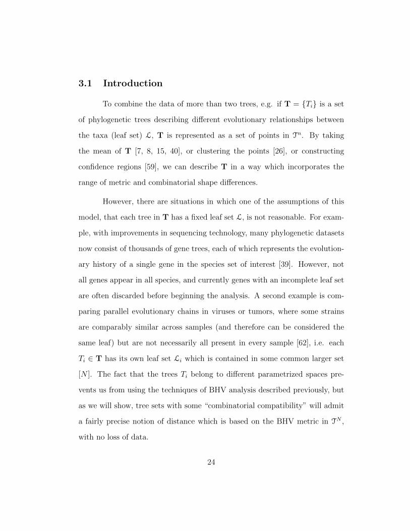
3.1 Introduction

To combine the data of more than two trees, e.g. if T = {Ti} is a set

of phylogenetic trees describing different evolutionary relationships between

the taxa (leaf set) L, T is represented as a set of points in Tn. By taking

the mean of T [7, 8, 15, 40], or clustering the points [26], or constructing

confidence regions [59], we can describe T in a way which incorporates the

range of metric and combinatorial shape differences.

However, there are situations in which one of the assumptions of this

model, that each tree in T has a fixed leaf set L, is not reasonable. For exam-

ple, with improvements in sequencing technology, many phylogenetic datasets

now consist of thousands of gene trees, each of which represents the evolution-

ary history of a single gene in the species set of interest [39]. However, not

all genes appear in all species, and currently genes with an incomplete leaf set

are often discarded before beginning the analysis. A second example is com-

paring parallel evolutionary chains in viruses or tumors, where some strains

are comparably similar across samples (and therefore can be considered the

same leaf) but are not necessarily all present in every sample [62], i.e. each

Ti ∈ T has its own leaf set Li which is contained in some common larger set

[N ]. The fact that the trees Ti belong to different parametrized spaces pre-

vents us from using the techniques of BHV analysis described previously, but

as we will show, tree sets with some “combinatorial compatibility” will admit

a fairly precise notion of distance which is based on the BHV metric in TN ,

with no loss of data.

24

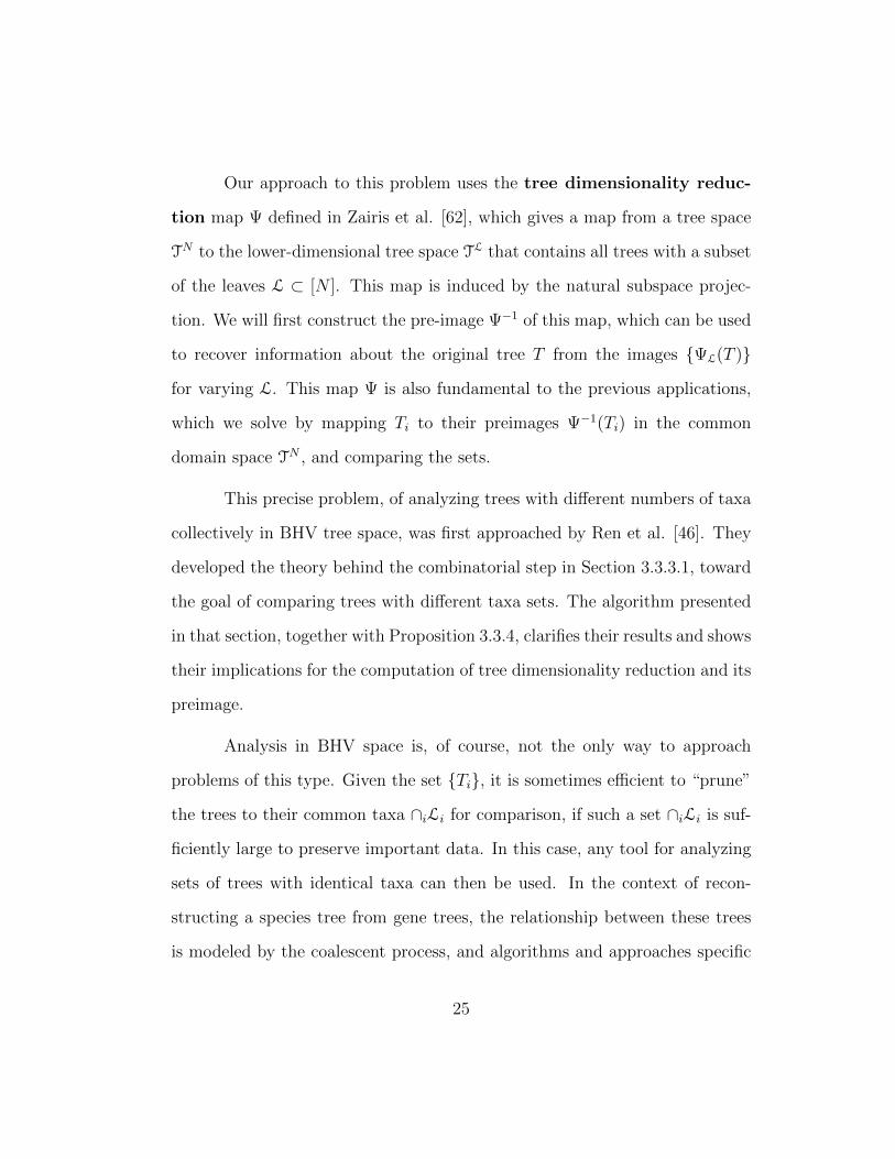
Our approach to this problem uses the tree dimensionality reduc-

tion map Ψ defined in Zairis et al. [62], which gives a map from a tree space

TN to the lower-dimensional tree space TL that contains all trees with a subset

of the leaves L ⊂ [N ]. This map is induced by the natural subspace projec-

tion. We will first construct the pre-image Ψ−1 of this map, which can be used

to recover information about the original tree T from the images {ΨL(T )}

for varying L. This map Ψ is also fundamental to the previous applications,

which we solve by mapping Ti to their preimages Ψ−1(Ti) in the common

domain space TN , and comparing the sets.

This precise problem, of analyzing trees with different numbers of taxa

collectively in BHV tree space, was first approached by Ren et al. [46]. They

developed the theory behind the combinatorial step in Section 3.3.3.1, toward

the goal of comparing trees with different taxa sets. The algorithm presented

in that section, together with Proposition 3.3.4, clarifies their results and shows

their implications for the computation of tree dimensionality reduction and its

preimage.

Analysis in BHV space is, of course, not the only way to approach

problems of this type. Given the set {Ti}, it is sometimes efficient to “prune”

the trees to their common taxa ∩iLi for comparison, if such a set ∩iLi is suf-

ficiently large to preserve important data. In this case, any tool for analyzing

sets of trees with identical taxa can then be used. In the context of recon-

structing a species tree from gene trees, the relationship between these trees

is modeled by the coalescent process, and algorithms and approaches specific

25

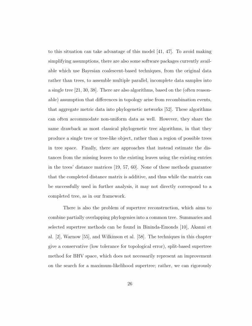
to this situation can take advantage of this model [41, 47]. To avoid making

simplifying assumptions, there are also some software packages currently avail-

able which use Bayesian coalescent-based techniques, from the original data

rather than trees, to assemble multiple parallel, incomplete data samples into

a single tree [21, 30, 38]. There are also algorithms, based on the (often reason-

able) assumption that differences in topology arise from recombination events,

that aggregate metric data into phylogenetic networks [52]. These algorithms

can often accommodate non-uniform data as well. However, they share the

same drawback as most classical phylogenetic tree algorithms, in that they

produce a single tree or tree-like object, rather than a region of possible trees

in tree space. Finally, there are approaches that instead estimate the dis-

tances from the missing leaves to the existing leaves using the existing entries

in the trees’ distance matrices [19, 57, 60]. None of these methods guarantee

that the completed distance matrix is additive, and thus while the matrix can

be successfully used in further analysis, it may not directly correspond to a

completed tree, as in our framework.

There is also the problem of supertree reconstruction, which aims to

combine partially overlapping phylogenies into a common tree. Summaries and

selected supertree methods can be found in Bininda-Emonds [10], Akanni et

al. [2], Warnow [55], and Wilkinson et al. [58]. The techniques in this chapter

give a conservative (low tolerance for topological error), split-based supertree

method for BHV space, which does not necessarily represent an improvement

on the search for a maximum-likelihood supertree; rather, we can rigorously

26

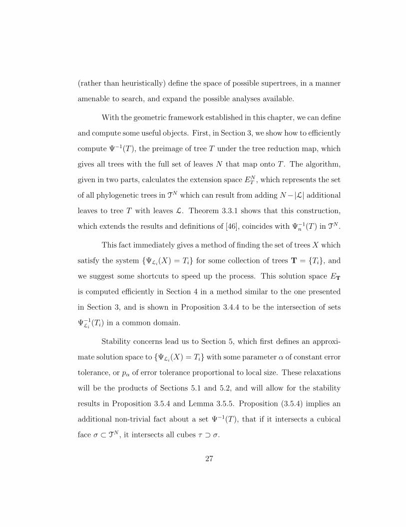
(rather than heuristically) define the space of possible supertrees, in a manner

amenable to search, and expand the possible analyses available.

With the geometric framework established in this chapter, we can define

and compute some useful objects. First, in Section 3, we show how to efficiently

compute Ψ−1(T ), the preimage of tree T under the tree reduction map, which

gives all trees with the full set of leaves N that map onto T . The algorithm,

given in two parts, calculates the extension space ENT , which represents the set

of all phylogenetic trees in TN which can result from adding N−|L| additional

leaves to tree T with leaves L. Theorem 3.3.1 shows that this construction,

which extends the results and definitions of [46], coincides with Ψ−1n (T ) in TN .

This fact immediately gives a method of finding the set of treesX which

satisfy the system {ΨLi(X) = Ti} for some collection of trees T = {Ti}, and

we suggest some shortcuts to speed up the process. This solution space ET

is computed efficiently in Section 4 in a method similar to the one presented

in Section 3, and is shown in Proposition 3.4.4 to be the intersection of sets

Ψ−1Li(Ti) in a common domain.

Stability concerns lead us to Section 5, which first defines an approxi-

mate solution space to {ΨLi(X) = Ti} with some parameter α of constant error

tolerance, or pα of error tolerance proportional to local size. These relaxations

will be the products of Sections 5.1 and 5.2, and will allow for the stability

results in Proposition 3.5.4 and Lemma 3.5.5. Proposition (3.5.4) implies an

additional non-trivial fact about a set Ψ−1(T ), that if it intersects a cubical

face σ ⊂ TN , it intersects all cubes τ ⊃ σ.

27

We use these error tolerance parameters for single trees, α and pα, to

define two parameters αT and pT measuring the degree of metric distortion

for a collection of trees T = {Ti} satisfying a combinatorial compatibility

condition. The parameters represent the minimum error tolerance (uniform

or proportional) necessary to construct a supertree from the {Ti}. These pa-

rameters will result from linear optimization problems related to the equations

defining the approximate solutions spaces, and can be directly computed using

the most efficient linear programming methods available.

3.2 Background

Unlike the previous chapter, the algorithm and results presented apply

to the space Tn, or TL, for any set of leaves L. This space embeds a phyloge-

netic tree according to the partition and weights of all of its edges, including

leaf edges as well as the internal edges that parametrize BHV. Since all trees

in BHVL have the same leaves, and therefore the same leaf partitions, we

can represent these leaf edge lengths globally with non-negative coordinates

(R≥0)|L|, and define tree space TL with this product

TL := BHVL × (R≥0)|L|

In this case, the cone point is the tree with no edges and all leaves identified into

a single point. Importantly, TL has all of the important features of BHVL: it

remains connected, globally non-positively curved, and contractible. As above,

when L = [n], we may alternatively write Tn for the space. The distance

28

dTL(·, ·): TL × TL → R can also be computed by a version of the algorithm of

Owen and Provan [45].

BHVL can then be expressed as a cone on LL based at 0 (hence the

name “cone point”), with the cone dimension parametrizing magnitude. De-

note the 1-skeleton of the link L1L. The global non-positive curvature condition

on BHVL implies that LL is a flag complex, meaning that each k-clique in L1L

bounds a k-simplex in LL, which corresponds uniquely to the orthant of di-

mension k spanned by the k splits. Thus, LL is recoverable from L1L, which

together encode all of the non-linearity of BHVL. In [46], and in the algorithm

presented in Section 3.3, L1L is used to calculate the (combinatorial) extension

objects GTs,n,ℓ and STs,n,ℓ.

3.2.1 Tree dimensionality reduction

A weighted graph, endowed with the shortest path metric, is a metric

space whose underlying set is the vertices of the graph. Acyclic graphs have

unique geodesics, and so a metric tree with n leaves can be equivalently con-

sidered as a metric on the set of n leaves, with distance between two leaves

given by the length of the unique path between them. A metric δ which arises

from a tree in this way is called an additive metric, and satisfies the four

point condition:

δ(a, b) + δ(c, d) ≤ max{δ(a, c) + δ(b, d), δ(a, d) + δ(b, c)}

for all leaves a, b, c, d.

29

The four point condition is also sufficient to determine additivity, which

in turn implies the existence of a unique tree realizing this metric [16]. The

additive distance matrix of a tree T with leaf set L = {ℓ1, ℓ2, ..., ℓn} is

denoted AT and is an n × n matrix where the (i, j)-th entry is δ(ℓi, ℓj), the

distance between leaves ℓi and ℓj in tree T .

A subspace of an additive metric space is additive, and additive sub-

spaces can be seen as forming subtrees. Tree dimensionality reduction

(TDR), as defined in [62], is a method of generating the tree for a subspace of

an additive metric space from the original metric tree, and for a more general

class of metric spaces called “nearly” additive. This work concerns strictly ad-

ditive metric spaces, although many algorithms exist to project nearly additive

spaces to tree approximations.

Definition 3.2.1. Let T be a tree with leaf set [N ] = {1, 2, . . . , N}, and

let L ⊂ [N ]. The tree dimensionality reduction map ΨL : T[N ] → TL

is the map sending T ∈ TN to the induced subtree spanned by the leaves

L, where the induced subtree contains the vertices and edges on the shortest

paths through T between the leaves in L, with each resulting degree 2 vertex v

and its incident edges (v, u1), (v, u2) with lengths ℓ1 and ℓ2 respectively, being

replaced by a single edge (u1, u2) with length ℓ1 + ℓ2. We refer to this process

as concatenation of (v, u1) and (v, u2).

Example 3.2.1. Starting with the tree on the left in Figure 3.1, tree dimen-

sionality reduction to the leaf set {1, 2, 3, 4} is performed by first pruning the

30

Figure 3.1: Left, a tree with 5 leaves. Center, the tree with leaf 5 and itsedge deleted, resulting in a degree two vertex (in red). Right, the tree afterconcatenating the two edges adjacent to the degree two vertex.

5th leaf and its leaf edge, which gives the center tree. This tree has a degree 2

vertex, in red, which is removed, its boundary edges concatenated, to produce

the final tree on the right.

We will also consider the related dimensionality reduction map on splits,

which we will refer to as projection. For a split P |P c on leaf set [N ], the

projection onto the leaf set L ⊂ [N ] is the split (P ∩ L)|(P c ∩ L). Note that

one of P ∩L or P c∩L may be empty, in which case the image is trivial. Since

the tree dimensionality map ΨL operating on tree T ∈ TN has the effect of

projecting all splits S = S(T ) onto the leaf set L, we will abuse notation and

use ΨL(S) to represent this combinatorial projection.

The following result states that the dimensionality reduction will act

on a tree naturally, when considered as an additive metric space.

Proposition 3.2.2 ([62, Proposition 4.4]). Let T be a tree with leaf set [N ] =

{1, 2, . . . , N}, and additive distance matrix AT . Let L ⊂ [N ], and define

31

(AT )L to be the submatrix of AT with rows and columns indexed by L. Then

AΨL(T ) = (AT )L.

Note that Proposition 3.2.2 implies that if L ⊂ L′ ⊂ [N ], then ΨL ◦

ΨL′ = ΨL on TN .

3.3 The Pre-Image of the Tree Dimensionality Reduc-tion Map

The aim of this section will be to algorithmically construct the preimage

of the tree dimensionality reduction map ΨL : TN → TL, for L ⊂ [N ], |L| = n.

We start with a binary tree T ∈ TL with edge lengths we for e ∈ E(T ), and

want to describe and compute the set of all trees T ∈ TN such that ΨL(T ) = T .

Since by Proposition 3.2.2 the distance of the leaves N\L to each other and to

the leaves L does not affect the distance between the leaves L, many different

tree topologies can map to T under ΨL. Thus it is not immediately obvious

how this set Ψ−1L (T ) should be described.

As this section demonstrates, one effective approach, which we call the

extension algorithm, is to:

1. Note that for any T ∈ TN , the topology of the image ΨL(T ) is completely

determined by the topology of T , and ΨL acts linearly on the E(T ) edge

weights in the orthant O(T ) in TN . Thus, for a fixed maximal orthant of

TN , ΨL restricts to a linear map M : R2N−3 → R2n−3. Any non-maximal

orthant is on the boundary of at least three maximal orthants, and the

32

linear map of any of these maximal orthants can be used.

2. Find the orthants with a topology T such that ΨL(T ) has the same

topology as T . By Proposition 3.3.4, these orthants can be determined

by individual and pairwise properties of their splits.

3. For a fixed orthant O, form the matrix MOT which encodes the way the

edges of trees in O concatenate under ΨL.

4. Find the positive solutions of the linear system of equations MOT x

O = w,

where w is the vector of edge weights in T , to determine the points

T ∼ xO ∈ O such that when ΨL is performed, all of the edges of T ∈ O

which concatenate to form an edge e ∈ T have weights summing to we.

5. Take the union of all of the orthant-wise solutions, which we call the

extension space ENT .

We will show that ENT = Ψ−1

L (T ) ⊂ TN , and that the resulting space

is connected, continuous, piecewise linear, of local dimension 2(N − n), and

computable in cubic time relative to its size.

Note that we will assume that T is binary, since an unresolved tree is

often used in biology when the underlying relationship of certain leaves or sub-

trees is not known. In such cases, the edge lengths near the unresolved vertex

would not necessarily represent the expected length of their corresponding split

in the true tree, which is the main assumption we are using. Thus we focus

33

on binary trees, and leave incorporating unresolved trees into this framework

for future work.

3.3.1 Extension by one leaf

To give some intuition for how the extension space relates to the original

tree, and to show the mechanics of the base case for later results, we first

examine the case where N = |L|+ 1. That is, we want to find the set of trees

Ψ−1L (T ) which have one additional leaf, labeled g.

Definition 3.3.1. Let Ψg : TN → TN\g be the tree dimensionality reduction

map which deletes leaf g ∈ [N ] and its adjacent edge, and concatenates the

two edges at leaf g’s attachment point. We will refer to this reduction as an

g-pruning.

The reverse of pruning a leaf g is attaching a new leaf g to the tree with

a new edge. We call this attachment operation grafting.

Definition 3.3.2. For a tree T ∈ TL, the tree T is a g-grafting of T if

L(T )\L(T ) = {g}, and Ψg(T ) = T .

In other words, a grafting of T consists of a tree identical to T , but

with one additional leaf g and its leaf edge eg. In considering the possibilities

for such a grafting, there are two independent choices: the non-negative length

of eg, and a point on T at which to graft the non-leaf end. The next lemma

shows the consequences of these two choices, and a bit more.

34

Lemma 3.3.1. For tree T ∈ TL and leaf g /∈ L, the space of g-graftings of T ,

denoted Ψ−1g (T ), is the direct product of R≥0 and a piecewise-linear connected

curve which is graph-isomorphic to T and which intersects a strict subset of

orthants each in a 1-dimensional linear curve.

Proof. Consider any tree T ∈ TL, leaf g /∈ L and length x ≥ 0. Recall that

E(T ) is the set of edges of tree T ∈ TL, with each edge e ∈ E(T ) having split

Pe and length we.

We can attach a new edge eg of length wg ending in leaf g to any point,

including an endpoint, on any edge of T to get a g-grafting of T . Thus the set

of g-graftings of T , Ψ−1g (T ), is not empty. For any T ∈ Ψ−1

g (T ), its additive

metric AT restricted to the leaves L is just the additive metric of T , AT . It

follows T can be completely characterized by two independent choices: the

choice of point on T for grafting, the space of which is graph-isomorphic to T ,

and a choice of length for the grafted leaf edge, which can be any non-negative

real number.

Let e ∈ E(T ) be the edge to which eg, which has split Pg = g|L, will be

grafted to form T . If we are grafting g to a vertex of T , then choose e to be

one of the edges adjacent to this vertex. For each edge f ∈ E(T )\e, the two

partitions of the leaves in the corresponding split Pf induce two subtrees of T ,

and edge e is completely contained in one of these subtrees. Add leaf g to the

partition of Pf corresponding to this subtree to get Pf , the corresponding split

in T . The split Pe becomes the splits PeL= Pe|(P c

e ∪ g) and PeR= (Pe∪ g)|P c

e

35

in T . If eg was grafted to an endpoint of e, then one of PeL, Pe

Rwill have zero

weight, but we will still include it here as a split for consistency. Thus T has

precisely the splits {Pf : f ∈ E(T )\e} ∪ Pg ∪ PeL ∪ Pe

R.

For each edge f ∈ E\e, the weight of split Pf in T is the same as the

weight of split Pf in T , since the edge corresponding to Pf projects to the edge

corresponding to Pf without distortion. Thus, we will represent the weight of

edge f in T by wf as well. Split Pg has weight wg, and let splits PeLand

PeRhave weights wL

e and wRe , respectively. Then the space of all T formed by

grafting leaf g to edge e is a two-parameter family satisfying we = wLe + wR

e ,

and wg, wLe , w

Re ≥ 0. Note that wg is a free parameter, and we = wL

e +wRe is the

equation of a line. Thus this solution space in this orthant is the direct product

of R≥0 with the line that intersects the orthant boundaries at wLe = 0, wR

e = we

and at wLe = we, w

Re = 0.

It remains to show that the lines given by wLe +wR

e = we in each orthant

are connected and graph isomorphic to tree T . Let e and e′ be two adjacent

edges in T , separated by vertex v. Edges e and e′ are compatible because they

exist in the same tree, and thus the intersection of one partition from each split

is empty. Without loss of generality (by temporarily renaming the partitions

if necessary), assume that Pe ∩ Pe′ = ∅. Then the case wLe = we, w

Re = 0

corresponds to a tree with splits PeL

= Pe|(P ce ∪ g), with weight we, and

Pe′ = Pe′|(P ce′ ∪ g), with weight we′ , as well as splits Pf , with weight wf , for

all f ∈ E(T )\{e, e′}, and Pg, with weight eg. The case wLe′ = we′ , w

Re′ = 0

corresponds to a tree with splits Pe′L= Pe′ |(P c

e′ ∪ g), with weight we′ , and

36

Pe = Pe|(P ce ∪ g), with weight we, as well as splits Pf , with weight wf , for

all f ∈ E(T )\{e, e′}, and Pg, with weight eg. But these split and weight

sets are identical, and thus the two line endpoints coincide. Since the two

of these line segments meet if and only if they correspond to attaching leaf

g to adjacent edges in e, we get that the piecewise-linear connected curve is

graph-isomorhpic to T .

Example 3.3.2. Suppose we have a tree T with labels {1, 2, 3, 5} as depicted in

Figure 3.2, with leaf edges having length {0.15, 0.3, 0.2, 0.25} respectively, and

interior edge length 0.2. The corresponding additive distance matrix (indexed

respectively) is given by

AT =

0 .65 .35 .6.65 0 .7 .55.35 .7 0 .65.6 .55 .65 0

Then the preimage Ψ−1

4(T ) is the product of the subspace of T5 depicted on the

right in Figure 3.2 (with leaf edge length for 1, 2, 3, 5 determined uniquely by

the point on Ψ4(T ) below) and the copy of R≥0 (not shown) representing the

“4”-leaf edge length. If we fix the length y of the 4 leaf, the (4, y)-grafting of T

is the subspace shown by a thick line, together with unique local leaf coordinates

(w1, w2, w3, w4, w5) = (0.15− x(14), 0.3− x(24), 0.2− x(34), y, 0.25− x(45))

where x(14), x(24), x(34), x(45) are the weights of splits (14), (24), (34), (45), re-

spectively, if that split exists in the tree, and 0 otherwise.

Because Figure 3.2 omits the dimensions for the leaf edges, the four line

segments corresponding to grafting g to a leaf edge appear to end mid-orthant.

37

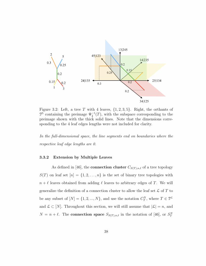
Figure 3.2: Left, a tree T with 4 leaves, {1, 2, 3, 5}. Right, the orthants ofT5 containing the preimage Ψ−1

4(T ), with the subspace corresponding to the

preimage shown with the thick solid lines. Note that the dimensions corre-sponding to the 4 leaf edges lengths were not included for clarity.

In the full-dimensional space, the line segments end on boundaries where the

respective leaf edge lengths are 0.

3.3.2 Extension by Multiple Leaves

As defined in [46], the connection cluster CS(T ),n,ℓ of a tree topology

S(T ) on leaf set [n] = {1, 2, . . . , n} is the set of binary tree topologies with

n + ℓ leaves obtained from adding ℓ leaves to arbitrary edges of T . We will

generalize the definition of a connection cluster to allow the leaf set L of T to

be any subset of [N ] = {1, 2, ..., N}, and use the notation CNT , where T ∈ TL

and L ⊂ [N ]. Throughout this section, we will still assume that |L| = n, and

N = n + ℓ. The connection space SS(T ),n,ℓ in the notation of [46], or SNT

38

in our notation, is the union of the closed orthants in TN that represent the

elements of CTN , i.e. a non-negative real orthant for every unweighted tree in

CTN under the normal identification of faces. The connection graph GS(T ),n,ℓ,

or with a change of notation, GNT , is the intersection of SN

T with the link L1N , in

which maximal cliques give elements of CNT . Ren et al. [46] and Lemma 3.3.5

below show that the edges of a connection graph are determined by normal

pairwise compatibility of splits in TN , which allows for quick computation of

CTN .

The connection space SNT can also be seen as the preimage in TN under

ΨL of the entire orthant represented by S(T ), namely Ψ−1L (O(T )). Similarly,

the connection graph GNT is the corresponding preimage of the complete n-

graph on S(T ). We are then interested in the subspace of SNT , restricted by

the edge lengths of T , which projects under tree dimensionality reduction to T .

This subspace will be a 2ℓ-dimensional linear submanifold supported in SNT .

In other words, once the combinatorics of the extended trees are calculated

through the connection cluster, we can use a set of (2n − 3) linear equations

parametrized by the edge lengths in T to constrain sums of fixed edges in TN

, and give the complete preimage Ψ−1L (T ).

3.3.3 Calculating the Metric Extension Space

In this section we will construct, for phylogenetic tree T ∈ Tn, the

subset ENT ⊂ ST

N ⊂ TN which results from gluing ℓ leaves of arbitrary length

to the metric tree T . The computation of the extension space ENT has two

39

steps:

The first step is the computation of SNT , via the method in [46] for

constructing GNT and CN

T . We will see that SNT is the preimage under ΨL of

the orthant containing T .

The second step introduces the constraint that under the action of ΨL

on SNT , the process of deleting and concatenating edge lengths as described

in Definition 3.2.1 yields T precisely. To find the trees which satisfy this

constraint, we solve a system of linear equations separately for each orthant

in SNT .

3.3.3.1 Combinatorial Step

As in the previous section, we let {Pe}e∈E(T ) be the splits of T (includ-

ing the leaf edges), with corresponding lengths {we}e∈E(T ). We will first state

the algorithm for computing the connection cluster CNT and give an example,

before proving correctness.

40

Algorithm 1 Computation of Connection Cluster

1: For each Pe, construct the set Qe of splits projecting to Pe by adding theℓ labels N\L to Pe or P

ce in all possible 2ℓ ways.

2: Take the union Q = ∪e∈E(T )Qe to get the vertices of the connection graphGN

T . Add an edge between each pair of vertices if and only if the twosplits are compatible, which can be checked by the condition given inDefinition 1.1.2.

3: Find all maximal (n + ℓ − 3) cliques in the subgraph of thick partitions,which is found by removing the leaf splits. Extend each maximal clique toinclude the leaf partitions, which are compatible with all other partitions,and return the corresponding set of cliques CN

T .

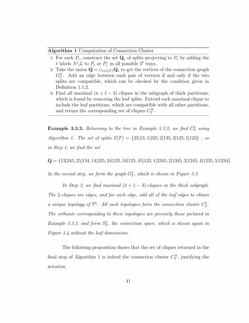
Example 3.3.3. Returning to the tree in Example 3.3.2, we find C5T using

Algorithm 1. The set of splits S(T ) = {25|13, 1|235, 2|135, 3|125, 5|123} , so

in Step 1, we find the set

Q = {13|245, 25|134, 14|235, 24|125, 34|125, 45|123, 1|2345, 2|1345, 3|1245, 4|1235, 5|1234}

In the second step, we form the graph G5T , which is shown in Figure 3.3.

In Step 3, we find maximal (4 + 1 − 3)-cliques in the thick subgraph.

The 2-cliques are edges, and for each edge, add all of the leaf edges to obtain

a unique topology of T5. All such topologies form the connection cluster C5T .

The orthants corresponding to these topologies are precisely those pictured in

Example 3.3.2, and form S5T , the connection space, which is shown again in

Figure 3.4 without the leaf dimensions.

The following proposition shows that the set of cliques returned in the

final step of Algorithm 1 is indeed the connection cluster CNT , justifying the

notation.

41

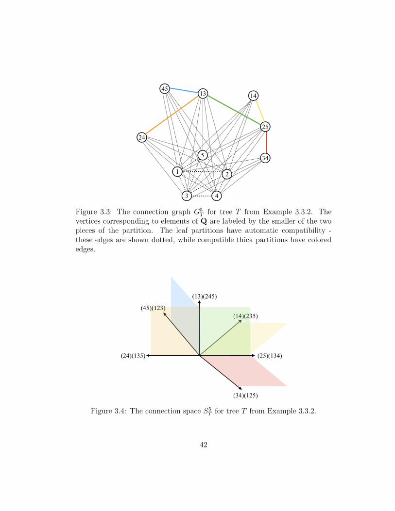
Figure 3.3: The connection graph G5T for tree T from Example 3.3.2. The

vertices corresponding to elements of Q are labeled by the smaller of the twopieces of the partition. The leaf partitions have automatic compatibility -these edges are shown dotted, while compatible thick partitions have colorededges.

Figure 3.4: The connection space S5T for tree T from Example 3.3.2.

42

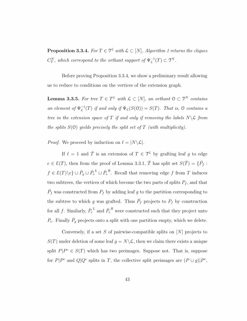
Proposition 3.3.4. For T ∈ TL with L ⊂ [N ], Algorithm 1 returns the cliques

CNT , which correspond to the orthant support of Ψ−1

L (T ) ⊂ TN .

Before proving Proposition 3.3.4, we show a preliminary result allowing

us to reduce to conditions on the vertices of the extension graph.

Lemma 3.3.5. For tree T ∈ TL with L ⊂ [N ], an orthant O ⊂ TN contains

an element of Ψ−1L (T ) if and only if ΨL(S(O)) = S(T ). That is, O contains a

tree in the extension space of T if and only if removing the labels N\L from

the splits S(O) yields precisely the split set of T (with multiplicity).

Proof. We proceed by induction on ℓ = |N\L|.

If ℓ = 1 and T is an extension of T ∈ TL by grafting leaf g to edge

e ∈ E(T ), then from the proof of Lemma 3.3.1, T has split set S(T ) = {Pf :

f ∈ E(T )\e} ∪ Pg ∪ PeL ∪ Pe

R. Recall that removing edge f from T induces

two subtrees, the vertices of which become the two parts of splits Pf , and that

Pf was constructed from Pf by adding leaf g to the partition corresponding to

the subtree to which g was grafted. Thus Pf projects to Pf by construction

for all f . Similarly, PeLand Pe

Rwere constructed such that they project unto

Pe. Finally Pg projects onto a split with one partition empty, which we delete.

Conversely, if a set S of pairwise-compatible splits on [N ] projects to

S(T ) under deletion of some leaf g = N\L, then we claim there exists a unique

split P |P c ∈ S(T ) which has two preimages. Suppose not. That is, suppose

for P |P c and Q|Qc splits in T , the collective split preimages are (P ∪ g)|P c,

43

P |(P c ∪ g), (Q ∪ g)|Qc, and Q|(Qc ∪ g). Then compatibility of P and Q in

T guarantees that precisely one of Q ∩ P,Qc ∩ P,Q ∩ P c, Qc ∩ P c is empty,

say without loss of generality Q ∩ P . Then (Q ∪ g)|Qc and (P ∪ g)|P c are

not compatible, because none of the four intersections of their partitions are

empty. Thus S contains only one of them. So for any pair of splits in T , there

are at most 3 preimage splits in S, and unique splits have distinct preimages,

so we conclude that there is a unique split in T with both preimages, i.e. the

set S must look precisely as above, {Pf : f ∈ E(T )\e} ∪ Pg ∪ PeL ∪ Pe

R, and

therefore we can construct T ∈ Ψ−1L (T ) uniquely by grafting the g-leaf edge to

the middle of edge e.

So we have the result for the ℓ = 1 case.

Then assume for induction that there exists T ∈ O ⊂ Tn+ℓ such that

ΨL(T ) = T , if and only if ΨL(S(O)) = S(T ). Then let O′ be an orthant

in Tn+ℓ+1. So then Ψn+ℓ(O′) is an orthant in Tn+ℓ, and applying the induc-

tive hypothesis, there exists T ′ ∈ Ψn+ℓ(O′) with ΨL(T

′) = T if and only if

ΨL(S(Ψn+ℓ(O′))) = S(T ). Since S(Ψn+ℓ(O

′)) = Ψn+ℓ(S(O′)) from the one-

step case, and ΨL(Ψn+ℓ(S(O′))) = ΨL(S(O

′)), giving us the forward direction.

For the reverse direction, we know that T ′ ∈ Ψn+ℓ(O′), which means that there

is some tree T ∈ O such that Ψn+ℓ(T ) = T ′ by the base case. For T then,

ΨL(T ) = ΨLΨn+ℓT = ΨLT′ = T , and the proof is complete.

Proof. (of Proposition 3.3.4) Suppose we have a maximal clique in GTN . Then

this clique represents a set of pairwise compatible splits. Since L1n is a flag

44

complex, these splits represents an orthant O in TN , of dimension correspond-

ing to the size of the clique. By Lemma 3.3.5, these splits projects to the splits

of T , so the orthant O contains elements of the extension space.

Conversely, suppose a tree T is in the extension space. Then by Lemma 3.3.5,

the splits of T are among the vertex set of GTN , and since T is a tree in TN , its

splits are compatible. Since compatibility is the condition for connectivity in

GTN as well as L1

n, T maps to a clique in GTN .

Proposition 3.3.6. The complexity of Algorithm 1 is O(23ℓn3).

Proof. In the first step of the algorithm, we do a simple enumeration, with

run time (2n − 3)2ℓ. The second step of removing duplicates and initializing

the graph is then O(22ℓn2), and to check compatibility is O(2n−3+ ℓ) in each

pair, so has O(22ℓn3). By [54], the run time of maximal clique enumeration is

O(|E| ∗ |V |), and from [46] we have that the vertex set has size 2ℓ(2n − 2) −

ℓ − n − 1, and the edge set size being at most the square of the size of the

vertex set, we have a O(23ℓn3) run time for clique enumeration. Thus step 3

dominates the other steps, which gives the result.

Note that while Algorithm 1 is fairly quick in n, it may be the case

that we have small fragments of large trees, implying a very dominant ℓ term.

In this case, Algorithm 1 is essentially reconstructing a large portion of Tn+ℓ,

and so there is not much improvement which can be made, since the solution

space itself is large. In the next section we will address a method for handling

small tree fragments among a set of tree fragments.

45

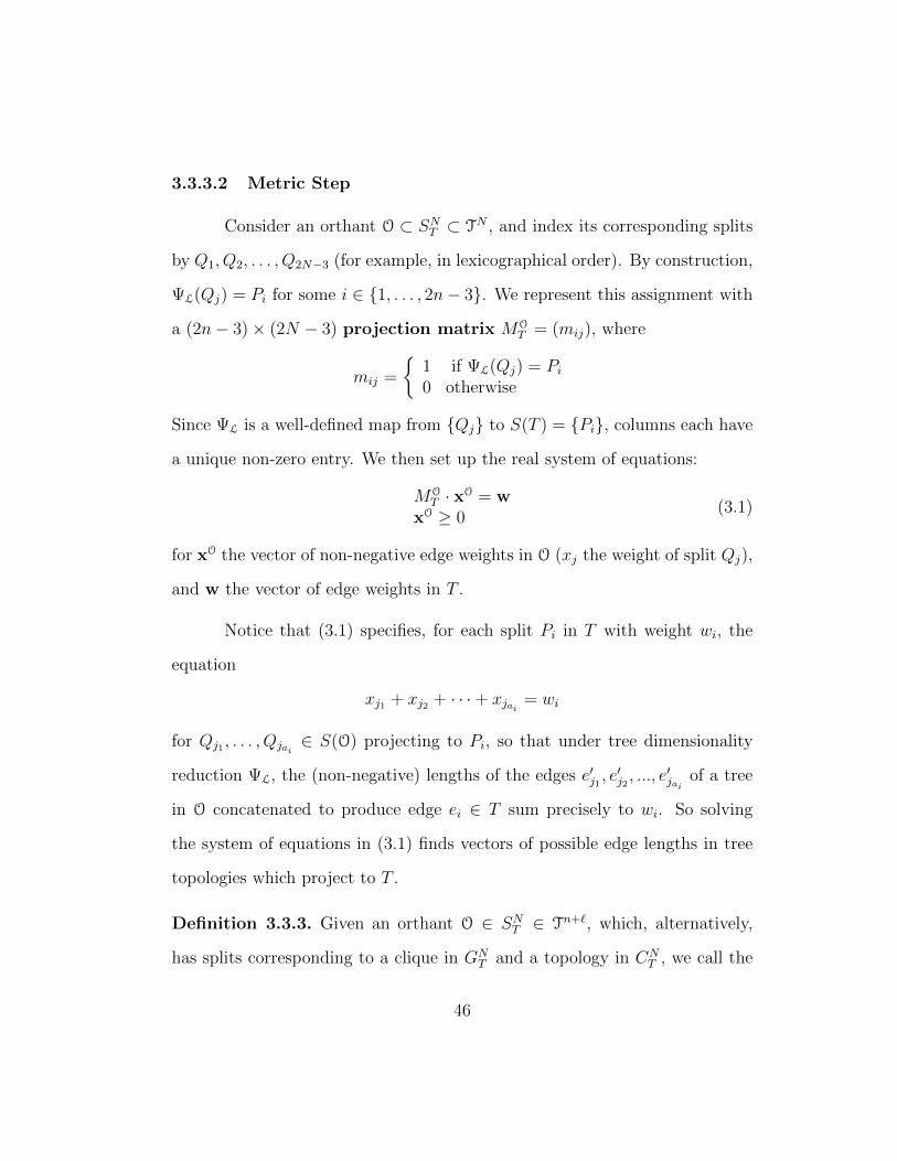
3.3.3.2 Metric Step

Consider an orthant O ⊂ SNT ⊂ TN , and index its corresponding splits

by Q1, Q2, . . . , Q2N−3 (for example, in lexicographical order). By construction,

ΨL(Qj) = Pi for some i ∈ {1, . . . , 2n− 3}. We represent this assignment with

a (2n− 3)× (2N − 3) projection matrix MOT = (mij), where

mij =

{1 if ΨL(Qj) = Pi

0 otherwise

Since ΨL is a well-defined map from {Qj} to S(T ) = {Pi}, columns each have

a unique non-zero entry. We then set up the real system of equations:

MOT · xO = w

xO ≥ 0(3.1)

for xO the vector of non-negative edge weights in O (xj the weight of split Qj),

and w the vector of edge weights in T .

Notice that (3.1) specifies, for each split Pi in T with weight wi, the

equation

xj1 + xj2 + · · ·+ xjai= wi

for Qj1 , . . . , Qjai∈ S(O) projecting to Pi, so that under tree dimensionality

reduction ΨL, the (non-negative) lengths of the edges e′j1 , e′j2, ..., e′jai of a tree

in O concatenated to produce edge ei ∈ T sum precisely to wi. So solving

the system of equations in (3.1) finds vectors of possible edge lengths in tree

topologies which project to T .

Definition 3.3.3. Given an orthant O ∈ SNT ∈ Tn+ℓ, which, alternatively,

has splits corresponding to a clique in GNT and a topology in CN

T , we call the

46

set of xO satisfying (3.1) the extension space of T in O, denoted EOT . The

extension space of T in TN is defined to be the union of extension spaces

over all orthants in the connection space:

ENT :=

⋃O∈SN

T

EOT .

Note that the image of Q = {Q1, . . . , Q2N−3} under tree dimensionality

reduction to L(T ) gives a partition of the set into precisely 2n−3 components,

because ΨL(Q) is well-defined and surjective on Pi’s. Because it is a partition

and wi > 0, we are guaranteed a solution of dimension∑

j mij − 1 to (3.1),

and a total solution space of dimension

2n−3∑i=1

((2N−3∑j=1

mij

)− 1

)=

2N−3∑j=1

2n−3∑i=1

mij− (2n−3) = (2N−3)− (2n−3) = 2ℓ.

The extension space ENT generalizes the single leaf extension case in that, after

the equations are solved for all orthants, the result is the direct product of a

piecewise-linear connected ℓ-manifold (intersecting a strict subset of orthants

each in an ℓ-dimensional linear subspace), with (R≥0)ℓ. Connectivity follows

from the consideration that if two orthants share a k-dimensional face, then

that face is represented as a k-clique in the connection graph, and the metric

extension space meets the face in a set of equations of precisely the same sort

on each side.

Proposition 3.3.7. For leaf set L ⊂ [N ], let T ∈ TL be a binary tree. The

extension space of T , ENT , is connected. Furthermore, for adjacent orthants

O1,O2 ⊂ SNT , EO1∩O2

T = EO1T ∩ O2 = O1 ∩ EO2

T .

47

Proof. For each orthant O ⊂ SNT , the extension space EO

T is connected, since

it is the solution of a linear system of equations, restricted to the non-negative

orthant. Any two adjacent orthants O1,O2 ⊂ SNT share some k-dimensional

boundary orthant, which corresponds to a k-clique in the connection graph.

Suppose the k splits in the clique are Qj1 , Qj2 , . . . , Qjk . Then any solutions xO1 ,

xO2 on the boundary only have non-zero weights for the splits Qj1 , Qj2 , . . . , Qjk .

Furthermore, since the projection of each Qj onto a unique split Pi in S(T )

does not depend on the orthant, when we remove the 0 weights from each

system of equations (MO1T · xO1 = w and MO2

T · xO2 = w), the two systems of

equations will now be identical. Therefore the intersection of EO1T and EO2

T is

precisely each of their intersections with the boundary orthant O1 ∩ O2.

Example 3.3.8. Returning to the tree T from Examples 3.3.2 and 3.3.3, based

on the projection Ψ4(Qj) which deletes the label “4”, we set up the following

linear system.

x25|134 + x13|245 = 0.2 = w13|25x24|135 + x2|1345 = 0.3 = w2|135x45|123 + x5|1234 = 0.25 = w5|123x14|235 + x1|2345 = 0.15 = w1|235x34|125 + x3|1245 = 0.2 = w3|125xj ≥ 0 ∀j

Without the leaf dimensions, the portion of the extension space pictured in

Example 3.4 is specified by the first equation and the non-negative constraints.

We now show that the extension space ENT defined in Definition 3.3.3 is

indeed the pre-image of the tree dimensionality reduction map ΨL : TN → TL.

Theorem 3.3.1. Let L ⊂ [N ] and T ∈ TL. Then ENT = Ψ−1

L (T ) ⊂ TN .

48

Proof. By construction and Proposition 3.3.4, ENT ⊂ SN

T , so ΨL(S(T )) =

S(T ) for each T ∈ ENT , i.e. EN

T and Ψ−1L (T ) intersect the same orthant set,

given by SNT . Furthermore, the procedure of dimension reduction as given in

Definition 3.2.1 guarantees that each edge ei ∈ E(ΨL(T )) will be obtained by

concatenating edges ej projecting to ei. Thus, to satisfy T = ΨL(T ), for a fixed

orthant O ∈ SNT , there is a fixed procedure of dimensionality reduction, and a

fixed set of splits {Qj}, each with weight wj, projecting to some Pi ∈ S(T ).

Therefore ΨL(T ) = T is equivalent to having∑

j:ΨL(Qj)=Piwj = wi for each

ei ∈ E(T ) with weight wi, which is precisely the condition specified by the

equations of EOT . Since EN

T and Ψ−1L (T ) agree in each orthant, we have the

result.

Complexity of the Extension Algorithm

If we restrict our computation to a single orthant, the matrixMOT can be

computed by calculating each ΨL(Qj) and matching with Pi, which is O(N).

Each such computation determines a column of MOT (with unique non-zero

entry in i-th position), so MOT is computed in O(N2).

The barrier to a polynomial time algorithm is the size of CNT , which by

[46] is

(2(n+ ℓ)− 5)!!

(2n− 5)!!∈ O(N ℓ).

These two estimates imply that computing all extension matrices is less than

quadratic in the support size of the space.

49

Proposition 3.3.9. The computation of the collection of matrices MOT is

O(N ℓ+2), which dominates the complexity of the previous steps in the extension

algorithm. Thus, the complexity of the extension algorithm is O(N ℓ+2).

Proof. The complexity of MOT follows from the above observations. Combined

with Proposition 3.3.6, the complete extension algorithm will be dominated

by N ℓ+2+23ℓn3, and so we have the complexity bound given in the statement.

For ℓ << n fixed, this is polynomial of degree ℓ+ 2.

The actual space of solutions, a convex affine polytope, can be presented

by its boundary vertices in each orthant; interior points can then be expressed

as convex combinations of boundary vertices. These convex combinations can

be computed, but there are a lot of them: since M is rank n, we expect around(Nn

)basic feasible solutions, which gives an estimate for boundary vertices. In

low dimensions, enumeration might be reasonable; there exist algorithms to

do this. In general, we will operate on this space in indirect ways.

Lemma 3.3.10. Let binary tree T ∈ TL with L ⊂ [N ], |L| = n, and |N\L| =

ℓ. To test whether a point x ∈ TN is in ENT , it is sufficient to check whether

ΨL(x) = T , which is O(N).

Proof. The first part is obvious from Theorem 3.2.1. For the complexity, we

note that in order to check the latter condition, we must perform dimensional-

ity reduction on x, which can be done in O(ℓ) from the tree representation of

50

x: each successive leaf removal results in at most one concatenation (see Defi-

nition 3.2.1). Then we must compare ΨL(x) to T . Since they are both binary

trees in TL, they each have 2n − 3 splits and, as graphs, 2n − 4 vertices. We

can therefore determine isometry by traversing the two trees simultaneously,

starting at the same leaf, which is O(n). Since N > n, ℓ, we have the result,

which is not tight.

For the more general statement of Lemma 3.3.10, see Proposition 3.4.5.

Remark 3.3.1. To find a point x in EOT which optimizes a linear function f(x) in

orthant O, standard linear programming methods will find a global solution in

polynomial time, with an average runtime ∼ N3B using the simplex method.

To estimate B, we note that matrices MOT will always be (2n− 3)× (2N − 3)

(binary) matrices, with 2n−3 edge lengths in floating point numbers, requiring

a total of O(Nn) bits, for a total average run time on the order of N4n.

3.3.4 Comparing extension spaces

One might hope that, as we have dTL(·, ·) which gives a well-defined

metric on TL, we can use this metric to define a meaningful distance between

ENT1

and ENT2

as sets. Though this calculation is possible, distances between

the sets E1 and E2 in TN do not produce a metric on extension spaces.

Remark 3.3.2. The distance function dEN : (ENT , EN

T ′) 7→ inf T∈ENT ,T ′∈EN

T ′dTN (T , T ′)

is not a pseudometric. To see this, take two distinct points T1,T2 in a non-

trivial extension space E; they are each trivial extensions of themselves, so they

51

are in the domain of the distance function, and there is a positive tree space

distance dTN (T1,T2) = dEN (T1,T2). However, each have inf T∈E(Ti, T ) = 0,

i = 1, 2, so inf T∈E(T1, T ) + inf T∈E(T2, T ) = 0, which violates the triangle in-

equality. Furthermore, dEN (E1, E2) = 0 and dEN (E2, E3) = 0 do not imply

dEN (E1, E3) = 0.

However, the vanishing of this quantity is meaningful, and corresponds

to a “compatibility” of trees:

Lemma 3.3.11. Let ENT and EN

T ′ be extension spaces of T ∈ TL and T ′ ∈ TL′,

respectively, where L,L′ ⊆ [N ]. Then dEN (ENT , EN

T ′) = 0 if and only if there

exists a tree T ∈ TN which contains all the splits of T and all the splits of T ′,

with lengths as in T and T ′.

Proof. If distance is zero then they intersect, since extension spaces are locally

affine. If they intersect, their intersection is non-empty, and we can choose

a tree T in this intersection. Then by Proposition 3.3.1, T projects to each

of T and T ′ under ΨL(T ) and ΨL(T ′), and so T contains a preimage of each

split P ∈ T, P ′ ∈ T ′, which separates the same leaves that P and P ′ do.

Furthermore by previous results we know that the pairwise distances between

leaves are preserved between T and T (and T ′ and T).

Then T can be seen as combining the information of T and T ′, as in

the case that T and T ′ are samples of a larger tree on different taxa subsets,

and this dEN (ENT , EN

T ′) = 0 case (and later, dEN (ENT , EN

T ′) < ϵ ) is what we

will explore in the next section.

52

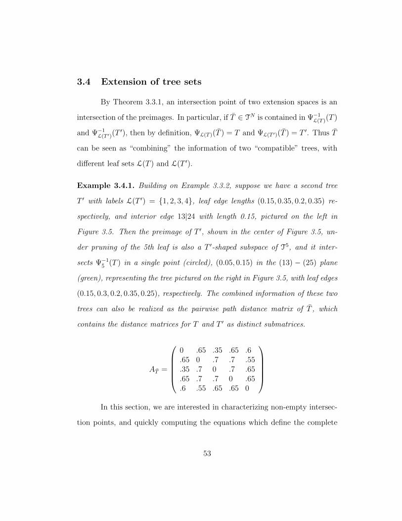
3.4 Extension of tree sets

By Theorem 3.3.1, an intersection point of two extension spaces is an

intersection of the preimages. In particular, if T ∈ TN is contained in Ψ−1L(T )(T )

and Ψ−1L(T ′)(T

′), then by definition, ΨL(T )(T ) = T and ΨL(T ′)(T ) = T ′. Thus T

can be seen as “combining” the information of two “compatible” trees, with

different leaf sets L(T ) and L(T ′).

Example 3.4.1. Building on Example 3.3.2, suppose we have a second tree

T ′ with labels L(T ′) = {1, 2, 3, 4}, leaf edge lengths (0.15, 0.35, 0.2, 0.35) re-

spectively, and interior edge 13|24 with length 0.15, pictured on the left in

Figure 3.5. Then the preimage of T ′, shown in the center of Figure 3.5, un-

der pruning of the 5th leaf is also a T ′-shaped subspace of T5, and it inter-

sects Ψ−15(T ) in a single point (circled), (0.05, 0.15) in the (13) − (25) plane

(green), representing the tree pictured on the right in Figure 3.5, with leaf edges

(0.15, 0.3, 0.2, 0.35, 0.25), respectively. The combined information of these two

trees can also be realized as the pairwise path distance matrix of T , which

contains the distance matrices for T and T ′ as distinct submatrices.

AT =

0 .65 .35 .65 .6.65 0 .7 .7 .55.35 .7 0 .7 .65.65 .7 .7 0 .65.6 .55 .65 .65 0

In this section, we are interested in characterizing non-empty intersec-

tion points, and quickly computing the equations which define the complete

53

Figure 3.5: Left, tree T (repeated from Figure 3.2) and a second tree T ′ withleaves {1, 2, 3, 4}. Center, the T -shaped subspace of Ψ−1

5(T ) and the T ′-shaped

subspace of Ψ−15(T ′), with their unique intersection circled. Right, the tree at

the intersection point of the two subspaces.

54

set. More generally, consider a collection of trees T = {T1, . . . , Tk} with any

leaf sets Lr, where |Lr| = nr. By fixing ℓr = N − nr we consider their tree

dimensionality reduction preimages Ψ−1Lr(Tr) collectively in TN . We can now

define generalizations of the

• connection cluster CNT := ∩rC

NTr,

• connection space SNT := ∩rS

NTr, and

• connection graph GNT := ∩rG

NTr.

These generalizations, CNT , SN

T , and GNT , correspond to the topologies in TN

which simultaneously extend S(Tr) for all Tr ∈ T.

As in Section 3, where T = {T}, we will first find CNT , and then find

solutions to a system of metric constraints, which gives the intersection ex-

tension space ENT := ∩rE

NTi. However, due to the high codimension of EN

Tr,

the extension space of T can be unstable under small treespace perturbations

of the Tr. In the next section, we will present two relaxations which will allow

for bounded independent perturbations of T1, . . . , Tk, which produces a neigh-

borhood of each ENTr

for transverse intersection. These relaxations also give

rise to two “measures of compatibility”, αT and pT, the minimum parameter

under two relaxation regimes giving a non-empty extension intersection. In

the final section, we will discuss methods for consolidating more diverse tree

topologies, which will choose orthants of highest likelihood for analysis.

55

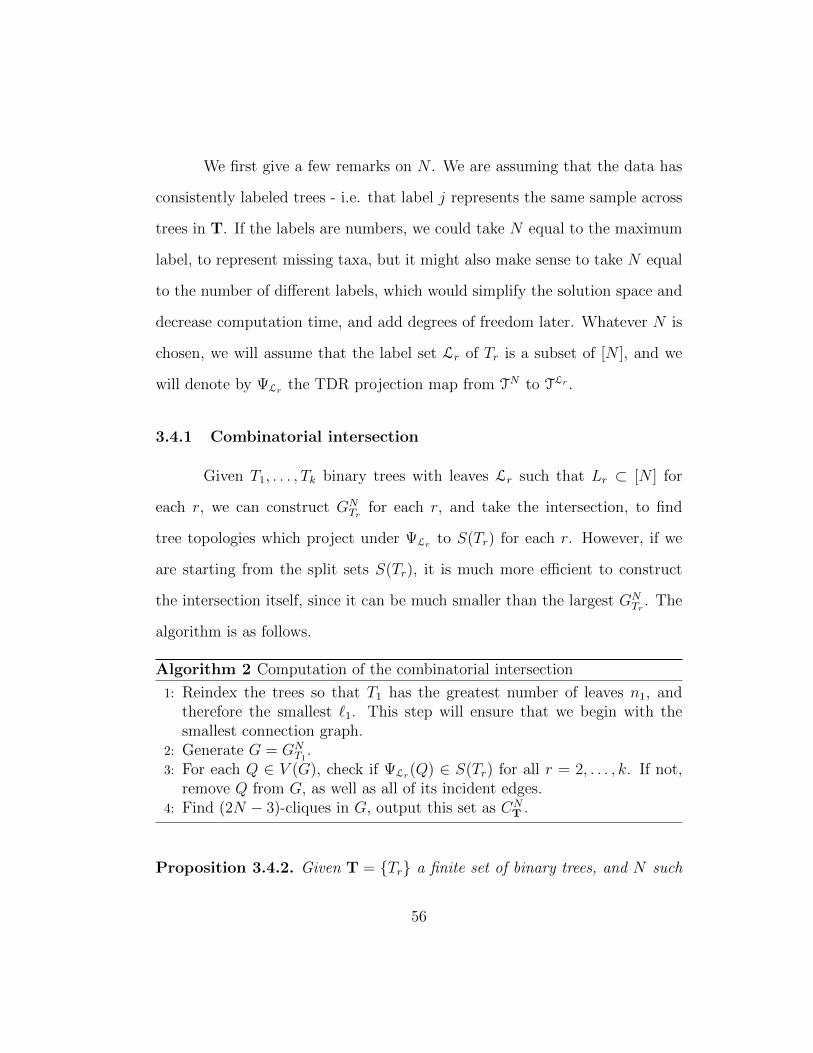
We first give a few remarks on N . We are assuming that the data has

consistently labeled trees - i.e. that label j represents the same sample across

trees in T. If the labels are numbers, we could take N equal to the maximum

label, to represent missing taxa, but it might also make sense to take N equal

to the number of different labels, which would simplify the solution space and

decrease computation time, and add degrees of freedom later. Whatever N is

chosen, we will assume that the label set Lr of Tr is a subset of [N ], and we

will denote by ΨLr the TDR projection map from TN to TLr .

3.4.1 Combinatorial intersection

Given T1, . . . , Tk binary trees with leaves Lr such that Lr ⊂ [N ] for

each r, we can construct GNTr

for each r, and take the intersection, to find

tree topologies which project under ΨLr to S(Tr) for each r. However, if we

are starting from the split sets S(Tr), it is much more efficient to construct

the intersection itself, since it can be much smaller than the largest GNTr. The

algorithm is as follows.

Algorithm 2 Computation of the combinatorial intersection

1: Reindex the trees so that T1 has the greatest number of leaves n1, andtherefore the smallest ℓ1. This step will ensure that we begin with thesmallest connection graph.

2: Generate G = GNT1.

3: For each Q ∈ V (G), check if ΨLr(Q) ∈ S(Tr) for all r = 2, . . . , k. If not,remove Q from G, as well as all of its incident edges.

4: Find (2N − 3)-cliques in G, output this set as CNT .

Proposition 3.4.2. Given T = {Tr} a finite set of binary trees, and N such

56

that Lr ⊂ [N ] for each r, then G =⋂

r GNTr, and therefore topology C ∈ CN

T if

and only if ΨLr(S(C)) = S(Tr) for each Tr.

Proof. By construction of the final graph G in Algorithm 2, V (G) consists of

splits Qj such that ΨLr(Qj) ∈ S(Tr) for each r. This is the vertex set of ∩rGNTr,

by construction. The edges of G, formed in Step 2 of Algorithm 2, come from

pairwise compatibility, which is independent of the original tree set. We know

also that compatibility determines adjacency equally for each GNTr, so that the

intersection of connection graphs is the full subgraph of the intersection of the

vertex set in L1N , and any edge which is present in GN

T1is present in all GTr

containing both endpoints. Therefore all edges of ∩rGNTr

are present in Step

2, and none are deleted, since their endpoints remain. So G = ∩rGNTr.

We can also note that if K is a maximal (2N − 3)-clique in G, then K

is also a maximal clique in each GNTr, and conversely, so that CN

T = ∩rCNTr.

Next, we note that by Proposition 3.3.4, topology C ∈ CNTr

if and only

if ΨLr(S(C)) = S(Tr). Then since CNT = ∩rC

NTr, it follows that C ∈ CN

T if and

only if ΨLr(N) = S(Tr) for each r.

Definition 3.4.1. We call a set T = {Tr} of binary trees combinatorially

compatible if CNT = ∅.

Definition 3.4.1 relates to edge compatibility (Definition 1.1.2), but edge

compatibility is not a special case of it. The requirement that the inputs be

binary trees would need to be generalized.

57

Proposition 3.4.3. If N · k < 22ℓ1, then the complexity of Algorithm 2 is

O(23ℓ1n31). If N ·k > 22ℓ1 , then it is O(2ℓ1n4

1k2). Either way, it is O(23ℓ1n4

1k2).

Proof. Reindexing the trees to put the tree with the most leaves first is O(k).

By Proposition 3.3.6, we have that Step 2 is O(22ℓ1n31). For Step 3, we iterate

through each of ∼ 2ℓ1n1 vertices, and for each, delete leaves to get down to

Lr (order N) and compare with the 2nr − 3 splits of Tr (order nr(2nr − 3) ∼

2n2r ⪅ 2n2

1). In total, then, Step 3 is O(2ℓ1n31Nk), and we can simplify to

O(2ℓ1n41k

2) by noting that N < k · n1. For Step 4, in the worst case, the size

of G is comparable to GNT1, so by Proposition 3.3.6, Step 4 is O(23ℓ1n3

1). If

N · k < 22ℓ1 , then Step 4 dominates. If not, Step 3 does.

3.4.2 Metric intersection

Given a binary topology C ∈ CNTwith splits Q1, . . . , QN−3, plus leaf

splits QN−2, . . . , Q2N−3, we have an 2ℓr-dimensional solution space for each

Tr, cut out by a set of equations

xm1 + xm2 + · · ·+ xmaj= wi

for each Pi ∈ S(Tr), i = 1, . . . , 2nr − 3. The collection of equations from all

Tr defines a solution space: either it is empty, or there is some linear subspace

of solutions, with dimension at most minr ℓr, which simultaneously satisfies

the collection of metric constraints. Unlike the single-tree extension case, this

system can be overdetermined, and have no solution in an orthant O ∈ SNT .

58

Definition 3.4.2. Let O ∈ SNT be an orthant in the intersection cluster, with

split lengths parametrized by respective coordinates (x1, . . . , x2N−3). Let MOTr

be the (2nr − 3)× (2N − 3) projection matrix of S to TLr . We then writeMO

T1

MOT2

...MO

Tk

xO =

w1

w2...wk

, xO ≥ 0 (3.2)

Then the solution space of xO satisfying (3.2) is denoted EOT. In (3.2),

the matrix on the left is denoted MOT for brevity, and the vector on the right

hand side wT, so expressing the equation more compactly, MOTxO = wT. The

intersection extension space of a collection T of trees is defined to be

ENT :=

⋃O∈ST

EOT,

where as before, N is taken to be the size of the total leaf set L(T) and

ℓr = N − nr for Tr ∈ T of size nr.

Note that when T = {T}, ENT = T , since N is set to L(T ), unless we

set a larger extension space, in which case ENT = EN

T , and so the results of

Section 3 are a special case of Definition 3.4.2 and the algorithm for computing

the intersection extension space.

Definition 3.4.3. Given a finite set of binary trees T, we call the set com-

patible if ET = ∅.

Trivially, for T ∈ TN , ΨL(T ) and ΨL′(T ) are compatible for L,L′ ⊂ [N ].

59

Proposition 3.4.4. For a collection T of trees with total leaf set of size N , the

intersection extension region of T is the intersection of the extension regions

of T ∈ T. That is, EOT =

⋂T∈T EO

T , ENT =

⋂T∈T EN

T .

Proof. From Proposition 3.4.2, we know that the orthant support of the inter-

section is the intersection of the orthant supports. Thus⋂T

ENT =

⋂T

⋃O

EOT =

⋃O

⋂T

EOT =

⋃O

EOT,

where the first equality is by definition of the intersection extension space,

the middle from finiteness of this union and intersection, and the last equality

follows from the fact that the intersection of real linear varieties is the vanishing

set of the collection of generating equations.

Complexity of computing the intersection extension space

As in Section 3, we can quickly do the operations that size allows.

For C = max{∑

Tr∈T 2nr − 3, N}, equation (3.2) is a C-dimensional system of

equations which can be set up in O(kN2) time. As before, this solution space

is cumbersome to describe enumeratively and quick to search.

Proposition 3.4.5. Given T = {Tr}r=1,...,k, [N ] = ∪Lr, and a tree T ∈ TN ,

the decision problem “Is T in ENT ?” can be solved in O(kN) time.

Proof. To answer the decision problem, it suffices to check, for each Tr ∈ T,

if ΨLr(T ) = Tr. By Lemma 3.3.10, each can be done in O(N) time, so the

problem is O(kN) time.

60

CNT may be substantially smaller than CN

T1(which is on the order of

N ℓ1), so a complete description may be possible. A starting point is linear

feasibility, i.e. determining if the system (3.2) has a solution, which, in contrast

to the single-tree case, is not automatically true. To solve, we introduce C slack

variables yP and a ℓ∞-norm variable α, and we minimize α subject to

(MO

T I)( xO

yP

)=(wT

)xma ≥ 0

α ≥ yP ≥ 0

(3.3)

This LP has an initial feasible solution: xO = 0, yP = wT, and minα = 0

if and only if there is an xO satisfying (3.2). This step takes as long as your

favorite LP solver, for example the simplex method, which will have an average

runtime of O(C5). In the next section we will investigate the case minα > 0.

For the LP formulation, skip to Section 3.5.1.1.

3.5 Relaxation

Since each ENTr

(for collection {Tr} as in Section 3.4 with fixed N =

nr + ℓr) is locally a submanifold of codimension 2nr − 3 in each orthant, for

nr + nr′ > N + 1, two extension manifolds will not intersect stably. Thus, a

small perturbation in two different projections of an N -tree may give the im-

pression of subtree incompatibility, as illustrated in Example 3.5.1 below. In

the language of our linear optimization problem (3.3), given a small amount

of sampling error in compatible trees, we may obtain an approximate solu-

tion with small, but positive, objective value. To ensure stability of inter-

61

section, we find a minimum amount of error αT, and find intersections of

αT-neighborhoods of the ENTr

in each orthant.

Example 3.5.1. Suppose tree T is as shown in Figure 3.5 and previous ex-

amples, and let T ′′ be tree T ′ in Figure 3.5 with the weight of the leaf 2 edge,

w2|134, being 0.3 instead of 0.35. Consider the 3-dimensional orthant O cor-

responding to splits 13|245, 25|134, and 2|1345. Then the intersection of ENT

with O is the solution to

x13|245 = 0.15

x2|1345 + x25|134 = 0.3 (3.4)

and the intersection of ENT ′′ with O is the solution to

x2|1345 = 0.3

x13|245 + x25|134 = 0.2 (3.5)

However, there is no common solution to both (3.4) and (3.5), as shown in

Figure 3.6. Thus the perturbation of the leaf 2 edge weight by 0.05 (or any

other small amount) in tree T ′′ means the extension spaces ENT and EN

T ′′ no

longer intersect.

3.5.1 Uniform α-relaxation

We can uniformly expand a single orthant of extension region EOT by

replacing each equation of the form

xm1 + xm2 + · · ·+ xmaj= wi

62

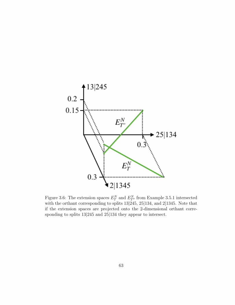
Figure 3.6: The extension spaces ENT and EN

T ′′ from Example 3.5.1 intersectedwith the orthant corresponding to splits 13|245, 25|134, and 2|1345. Note thatif the extension spaces are projected onto the 2-dimensional orthant corre-sponding to splits 13|245 and 25|134 they appear to intersect.

63

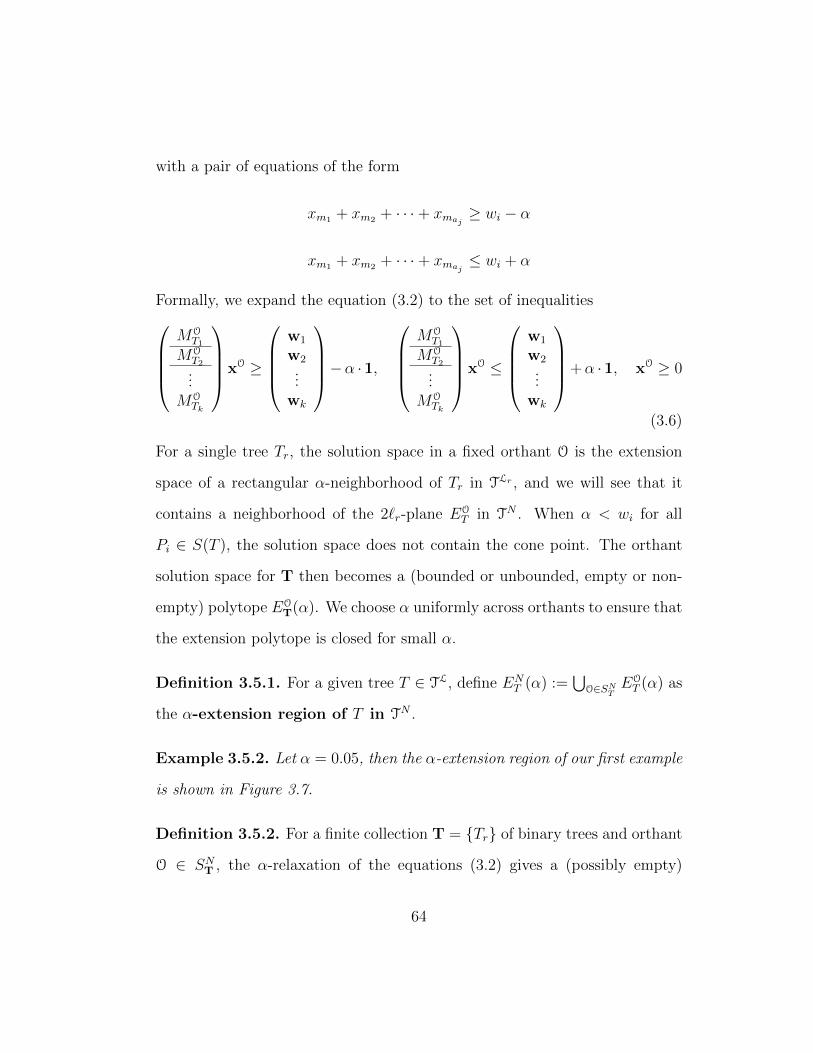
with a pair of equations of the form

xm1 + xm2 + · · ·+ xmaj≥ wi − α

xm1 + xm2 + · · ·+ xmaj≤ wi + α

Formally, we expand the equation (3.2) to the set of inequalitiesMO

T1

MOT2

...MO

Tk

xO ≥

w1

w2...wk

−α ·1,

MO

T1

MOT2

...MO

Tk

xO ≤

w1

w2...wk

+α ·1, xO ≥ 0

(3.6)

For a single tree Tr, the solution space in a fixed orthant O is the extension

space of a rectangular α-neighborhood of Tr in TLr , and we will see that it

contains a neighborhood of the 2ℓr-plane EOT in TN . When α < wi for all

Pi ∈ S(T ), the solution space does not contain the cone point. The orthant

solution space for T then becomes a (bounded or unbounded, empty or non-

empty) polytope EOT(α). We choose α uniformly across orthants to ensure that

the extension polytope is closed for small α.

Definition 3.5.1. For a given tree T ∈ TL, define ENT (α) :=

⋃O∈SN

TEO

T (α) as

the α-extension region of T in TN .

Example 3.5.2. Let α = 0.05, then the α-extension region of our first example

is shown in Figure 3.7.

Definition 3.5.2. For a finite collection T = {Tr} of binary trees and orthant

O ∈ SNT , the α-relaxation of the equations (3.2) gives a (possibly empty)

64

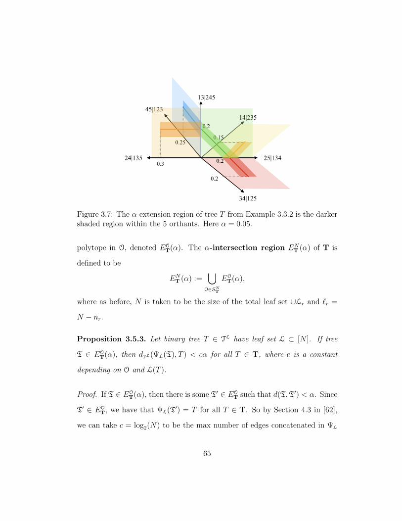
Figure 3.7: The α-extension region of tree T from Example 3.3.2 is the darkershaded region within the 5 orthants. Here α = 0.05.

polytope in O, denoted EOT(α). The α-intersection region EN

T (α) of T is

defined to be

ENT (α) :=

⋃O∈SN

T

EOT(α),

where as before, N is taken to be the size of the total leaf set ∪Lr and ℓr =

N − nr.

Proposition 3.5.3. Let binary tree T ∈ TL have leaf set L ⊂ [N ]. If tree

T ∈ EOT(α), then dTL(ΨL(T), T ) < cα for all T ∈ T, where c is a constant

depending on O and L(T ).

Proof. If T ∈ EOT(α), then there is some T′ ∈ EO

T such that d(T,T′) < α. Since

T′ ∈ EOT, we have that ΨL(T

′) = T for all T ∈ T. So by Section 4.3 in [62],

we can take c = log2(N) to be the max number of edges concatenated in ΨL

65

acting on S(TN).

Note that ENT (α) is not defined as an α-neighborhood of EN

T , but its

restriction to each orthant in SNT is an α-neighborhood in that orthant. Fur-

thermore, for small α, ENT (α) is closely related to the neighborhood.

Proposition 3.5.4. Let T ∈ TL be a binary tree with leaf set L ⊂ [N ]. For

α < log2(N)−1mine∈E(T ) we, ENT (α) contains the α-neighborhood of EN

T in TN .

Proof. The α-neighborhood Nα := Nα(ENT ) ⊂ TN is path-connected. Suppose

T ∈ Nα\ENT (α). Since Nα ∩ O = EN

T (α) for O ⊂ SNT , we conclude that T /∈ O

for any orthant of the connection space, so the orthant O′ containing T does

not contain a preimage of some edge e′ ∈ E(T ), i.e. e′ /∈ ΨL(S(O)). Since

the neighborhood is path-connected though, between T and ENT there is some

geodesic path γ contained in Nα, corresponding to a deformation of T to some

tree T ∈ ENT .

Consider the image of γ under ΨL. ΨL(T) does not have edge e′, so

ΨL(γ) must have length at least the length of the projection to e′. Therefore

the length of ΨL(γ) must be greater than α since the e′ component of the path

has length at least we′ ≥ minewe > log2(N)α. By [61] geodesic lengths grow

by at most log2(N) under ΨL, which implies T /∈ Nα, a contradiction.

Lemma 3.5.5. Let T = {Tr} be a finite set of binary trees in TN , each with

leaf set L(Tr) ⊂ [N ]. If α1 < α2, then ENT (α1) ⊂ EN

T (α2). For T, T ′ ∈ TL

with dTL(T, T ′) < min{α, log2(N)−1minej∈T wj}, we have the inclusion ENT ′ ⊂

ENT (α).

66

Proof. The first statement is clear from construction. For the second, if

dTL(T, T ′) < minwj/ log(N), then we have that T ′ has the same split set as T ,

with w′j the corresponding lengths. Each w′

j < wj + dTL(T, T ′) < wj + α, and

similarly w′j > wj−dTL(T, T ′) > wj−α, so solutions to xm1+xm2+· · ·+xmaj

=

w′j satisfy both inequalities.

Definition 3.5.3. For a finite, combinatorially compatible collection T of

trees {Tr}, each with leaf set L(Tr) ⊂ [N ], and a given orthant O ∈ SNT ,

we denote by αOT the infimum of α such that EO

T(α) is non-empty. Then the

intersection parameter αT := minO αOT.

If T can be obtained from a single N -tree by deleting subsets of the

leaves, then αT = 0. We also have a natural upper bound on αOT given by

the length of the longest edge in T (so that ENT (α) contains all EN

T (α)), so

αOT is guaranteed to be finite. The parameter αT represents minimum amount

the preimages of the trees Tr must be perturbed to have a metric solution,

assuming combinatorial compatibility.

3.5.1.1 Computing αT

When the system of equations (3.3) has a non-zero optimal solution,

we conclude that (3.2) had no solutions in that orthant, but we also obtain a

valuable by-product: a measure of the degree to which the extension spaces

ENTr

miss each other. For a solution xO,yP to (3.3), for each r = 1, . . . , k

we have a unique subset (yP )r ⊂ yP , satisfying only the system of equations

67

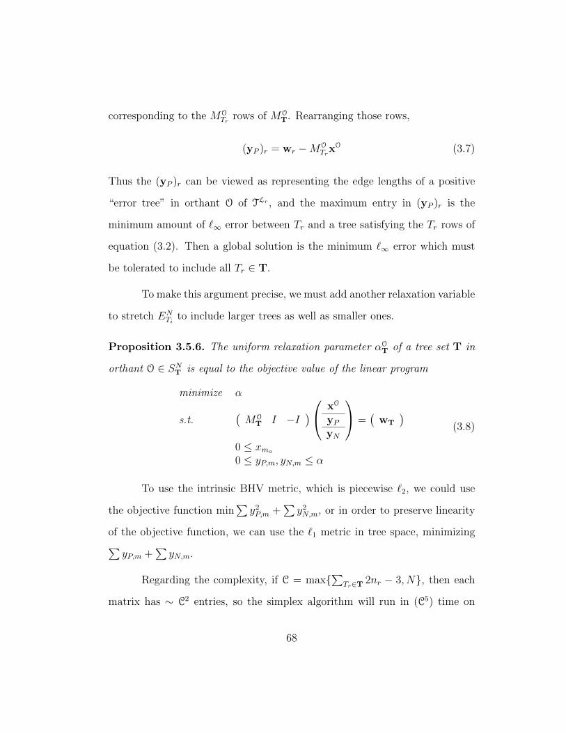
corresponding to the MOTr

rows of MOT. Rearranging those rows,

(yP )r = wr −MOTrxO (3.7)

Thus the (yP )r can be viewed as representing the edge lengths of a positive

“error tree” in orthant O of TLr , and the maximum entry in (yP )r is the

minimum amount of ℓ∞ error between Tr and a tree satisfying the Tr rows of

equation (3.2). Then a global solution is the minimum ℓ∞ error which must

be tolerated to include all Tr ∈ T.

To make this argument precise, we must add another relaxation variable

to stretch ENTi

to include larger trees as well as smaller ones.

Proposition 3.5.6. The uniform relaxation parameter αOT of a tree set T in

orthant O ∈ SNT is equal to the objective value of the linear program

minimize α

s.t.(MO

T I −I) xO

yP

yN

=(wT

)0 ≤ xma

0 ≤ yP,m, yN,m ≤ α

(3.8)

To use the intrinsic BHV metric, which is piecewise ℓ2, we could use

the objective function min∑

y2P,m +∑

y2N,m, or in order to preserve linearity

of the objective function, we can use the ℓ1 metric in tree space, minimizing∑yP,m +

∑yN,m.

Regarding the complexity, if C = max{∑

Tr∈T 2nr − 3, N}, then each

matrix has ∼ C2 entries, so the simplex algorithm will run in (C5) time on

68

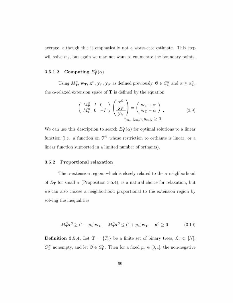
average, although this is emphatically not a worst-case estimate. This step

will solve αT, but again we may not want to enumerate the boundary points.

3.5.1.2 Computing ENT (α)

Using MOT, wT, x

O, yP , yN as defined previously, O ∈ SNT and α ≥ αS

T,

the α-relaxed extension space of T is defined by the equation

(MO

T I 0MO

T 0 −I

) xO

yP

yN

=

(wT + αwT − α

)xma , ym,P , ym,N ≥ 0

. (3.9)

We can use this description to search ENT (α) for optimal solutions to a linear

function (i.e. a function on TN whose restriction to orthants is linear, or a

linear function supported in a limited number of orthants).

3.5.2 Proportional relaxation

The α-extension region, which is closely related to the α neighborhood

of ET for small α (Proposition 3.5.4), is a natural choice for relaxation, but

we can also choose a neighborhood proportional to the extension region by

solving the inequalities

MOTx

O ≥ (1− pα)wT, MOTx

O ≤ (1 + pα)wT, xO ≥ 0 (3.10)

Definition 3.5.4. Let T = {Tr} be a finite set of binary trees, Lr ⊂ [N ],

CNT nonempty, and let O ∈ SN

T . Then for a fixed pα ∈ [0, 1], the non-negative

69

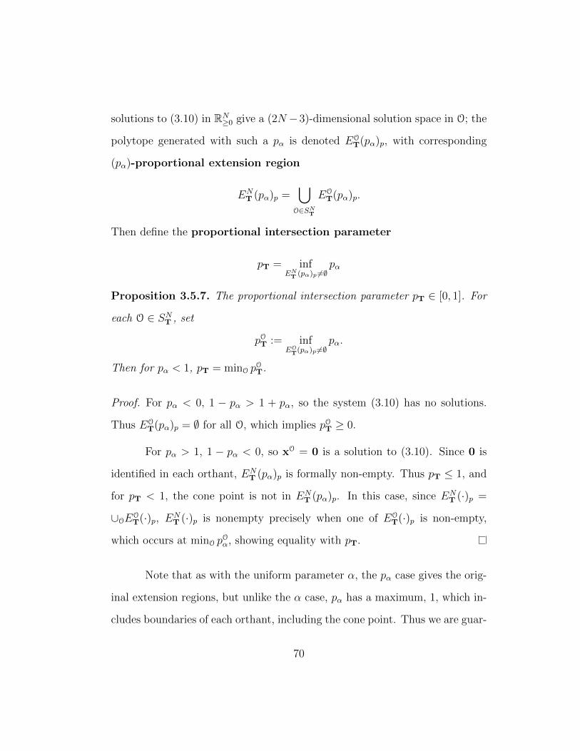
solutions to (3.10) in RN≥0 give a (2N −3)-dimensional solution space in O; the

polytope generated with such a pα is denoted EOT(pα)p, with corresponding

(pα)-proportional extension region

ENT (pα)p =

⋃O∈SN

T

EOT(pα)p.

Then define the proportional intersection parameter

pT = infEN

T (pα)p =∅pα

Proposition 3.5.7. The proportional intersection parameter pT ∈ [0, 1]. For

each O ∈ SNT , set

pOT := infEO

T(pα)p =∅pα.

Then for pα < 1, pT = minO pOT.

Proof. For pα < 0, 1 − pα > 1 + pα, so the system (3.10) has no solutions.

Thus EOT(pα)p = ∅ for all O, which implies pOT ≥ 0.

For pα > 1, 1 − pα < 0, so xO = 0 is a solution to (3.10). Since 0 is

identified in each orthant, ENT (pα)p is formally non-empty. Thus pT ≤ 1, and

for pT < 1, the cone point is not in ENT (pα)p. In this case, since EN

T (·)p =

∪OEOT(·)p, EN

T (·)p is nonempty precisely when one of EOT(·)p is non-empty,

which occurs at minO pOα, showing equality with pT.

Note that as with the uniform parameter α, the pα case gives the orig-

inal extension regions, but unlike the α case, pα has a maximum, 1, which in-

cludes boundaries of each orthant, including the cone point. Thus we are guar-

70

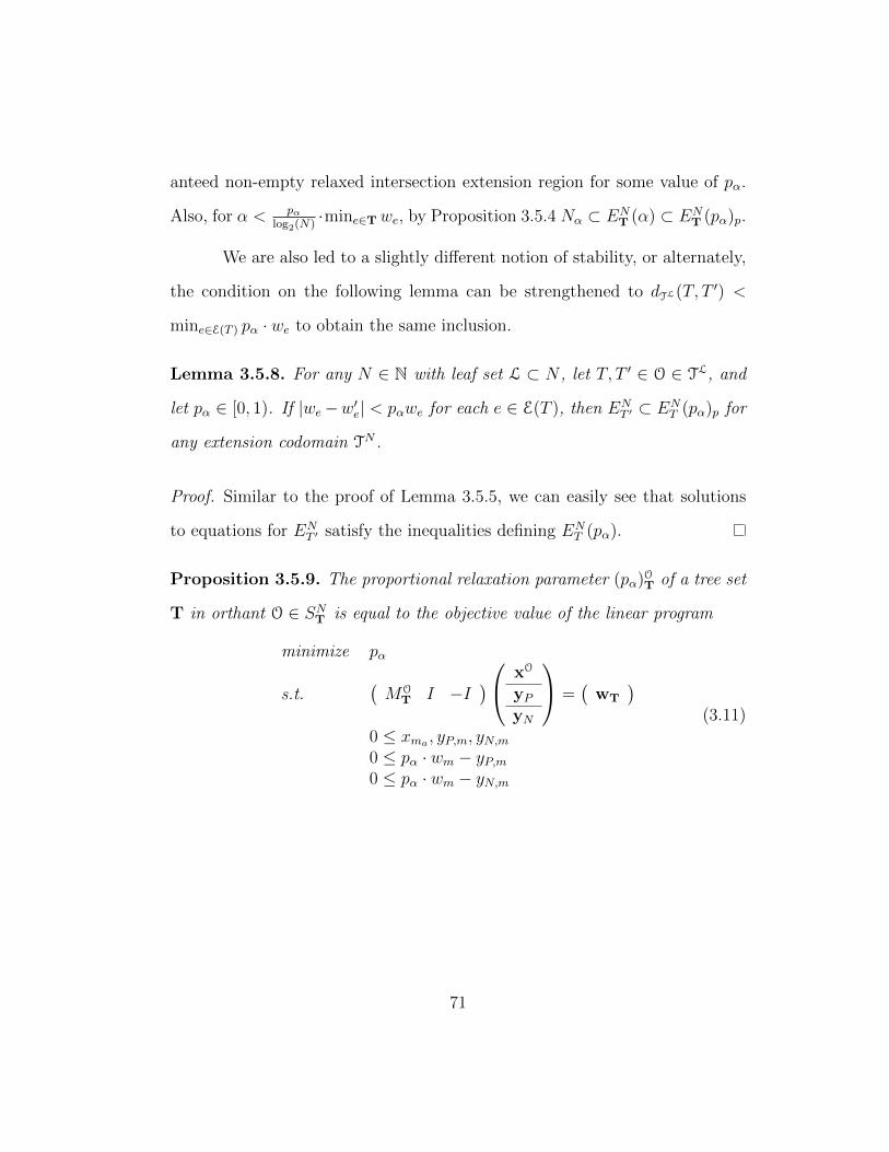
anteed non-empty relaxed intersection extension region for some value of pα.

Also, for α < pαlog2(N)

·mine∈Twe, by Proposition 3.5.4 Nα ⊂ ENT (α) ⊂ EN

T (pα)p.

We are also led to a slightly different notion of stability, or alternately,

the condition on the following lemma can be strengthened to dTL(T, T ′) <

mine∈E(T ) pα · we to obtain the same inclusion.

Lemma 3.5.8. For any N ∈ N with leaf set L ⊂ N , let T, T ′ ∈ O ∈ TL, and

let pα ∈ [0, 1). If |we −w′e| < pαwe for each e ∈ E(T ), then EN

T ′ ⊂ ENT (pα)p for

any extension codomain TN .

Proof. Similar to the proof of Lemma 3.5.5, we can easily see that solutions

to equations for ENT ′ satisfy the inequalities defining EN

T (pα).

Proposition 3.5.9. The proportional relaxation parameter (pα)OT of a tree set

T in orthant O ∈ SNT is equal to the objective value of the linear program

minimize pα

s.t.(MO

T I −I) xO

yP

yN

=(wT

)0 ≤ xma , yP,m, yN,m

0 ≤ pα · wm − yP,m0 ≤ pα · wm − yN,m

(3.11)

71

Chapter 4

Manifold Learning and Dimensionality

Reduction for Non-trivial Topology

In this chapter we give exposition of some techniques in manifold learn-

ing, and outline three new heuristic methods currently in development for pre-

serving various topological features in the process. The main output will be

a set of non-linear projections for the manifold depending on the local distri-

butions of data - after fitting a mixture of locally flat models, we group the

local subspaces based on topological data and align each in low-dimensional

Euclidean space or on a sphere.

4.1 Introduction

Given a set of sample points Y = (y1, . . . , yN) ⊂ Rn, and a suspi-

cion that they may lie on or near some lower-dimensional embedded manifold

M ⊂ Rn, manifold learning either attempts to construct a non-linear dimen-

sionality reduction map (NLDR), or to provide a description of the best-fit

manifold for the data, freely or within a parametrized family. Manifold learn-

ing is a very active and applied area, but most techniques assume that the

manifold in question is contractible or relatively flat, often trying to find the

72

best representation in R2 or R3 independent of structure.

There are some notable exceptions. Riemannian manifold learning [37],

for example, embeds a base tangent plane isometrically and extends iteratively

outward, minimizing distortion to angle and geodesic length. This can be done

locally at points of interest or globally at the centroid.

By fitting not just the manifold, but the tangent bundle, we move to-

ward additional geometric structure. If M is flat, meaning with zero curvature

at every point, then a map from the tangent bundle to Rd gives the unique

flat connection, meaning parallel transport along curves is path-independent

and given by translation of the vector in Rd. Tangent space alignment [63]

uses local PCA and a technique similar to the least squares method of Section

4.5.1 to align local frames in Rd. This also works to preserve local geometry

and global structure, although [63], like manifold charting [13], assembles a

single flat chart. This works best if M is close to a compact subset of a linear

affine subspace in Rn.

Recently, Scoccola and Perea have developed a technique of approx-

imating Euclidean vector bundles using nearest-neighbors PCA and the or-

thogonal Procrustes alignment between pairs of approximate tangent spaces

[49]. This allows them to specify an orthogonal structure group, and to go on

to define approximate cocycle conditions, estimates of characteristic classes,

and a reconstruction theorem that allows for precise guarantees on homotopy

equivalence.

73

In all of these techniques there is a tradeoff between topological fidelity

and speed of computation1, and we aim toward bridging the gap.

Our approach is to extend the least squares alignment of [13] to the

case where M is

• a sphere

• non-contractible, with high reach and bounded curvature

• a union of contractible manifolds, not necessarily disjoint, of possibly

mixed dimension, intersecting transversely.

Using the same flat tangent space alignment optimization, we patch together

the local linear subspace arrangements resulting from the symmetric block

decomposition of Kileel and Pereira [33]. Following their GPCA algorithm,

we decompose the 2n-th data moment, where n ≥ 2, to robustly approximate

the local structure, which may be a transverse intersection of tangent spaces

of various dimension.

We also generalize the alignment algorithm to optimize connections

on a sphere of dimension d. A theorem of Kobayashi states that the Levi-

Civita connection on a smooth surface is the pullback under the Gauss map

of the Levi-Civita connection on the sphere. In projecting to the sphere with

1For example, the Niyogi-Smale-Weinberger result guaranteeing homotopy equivalence ofthe Cech complex requires quite high amounts of samples, which then create an intractibleload on the already computationally intensive persistent-homology algorithms.[43]

74

minimal distortion, we construct a discrete dimension-reduced approximation

of the Gauss map, which will give us a dimension-reduced approximation of

the Levi-Civita connection on an unknown manifold, which may very well have

torsion/holonomy.

Our procedure assumes that Y lies on some unknown compact mani-

fold M ⊂ Rn, with bounded reach and curvature. We will construct a (proba-

bilistic) open cover consisting of ellipsoidal distributions in Rn, together with

projection maps to local coordinates Uj ⊂ Rd, and find a small set of relatively

flat charts to cover M, which can be quickly aligned in Rd.

1. (Section 4.3.3) Estimate the intrinsic dimension[s] d of the data locally.

2. Estimate the embedded tangent bundle structure with a Gaussian mix-

ture model {πj,N(µj,Σj)}j=1,...,k. Sections 4.2 and 4.3 give different

methods, for manifolds and stratified/mixed manifolds, respectively, or

any GMM approximation will suffice. In either case, we take the d princi-

pal components of the local model to represent the tangent plane TµjM.

3. Instead of set inclusion determining membership yi ∈ Uj, we compute

stochastic membership weights from the density functions of our cover.

This is a significant relaxation of the notion of an open set which accounts

for both off-manifold and on-manifold noise. To each point y ∈ Y,

calculate pky recording the relative likelihood that y belongs to chart k.

This is either the normalization of a vector of density functions fk(y) for

75

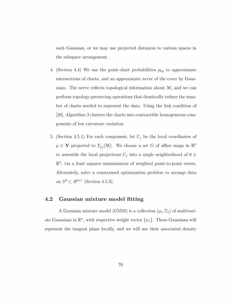
each Gaussian, or we may use projected distances to various spaces in

the subspace arrangement.

4. (Section 4.4) We use the point-chart probabilities pky to approximate

intersections of charts, and an approximate nerve of the cover by Gaus-

sians. The nerve reflects topological information about M, and we can

perform topology-preserving operations that drastically reduce the num-

ber of charts needed to represent the data. Using the link condition of

[20], Algorithm 3 clusters the charts into contractible homogeneous com-

ponents of low curvature variation.

5. (Section 4.5.1) For each component, let Uj be the local coordinates of

y ∈ Y projected to Tµj(M). We choose a set G of affine maps in Rd

to assemble the local projections Uj into a single neighborhood of 0 ∈

Rd, via a least squares minimization of weighted point-to-point errors.

Alternately, solve a constrained optimization problem to arrange data

on Sd ⊂ Rd+1 (Section 4.5.3).

4.2 Gaussian mixture model fitting

A Gaussian mixture model (GMM) is a collection (µi,Σi) of multivari-

ate Gaussians in Rn, with respective weight vector {wi}. These Gaussians will

represent the tangent plane locally, and we will use their associated density

76

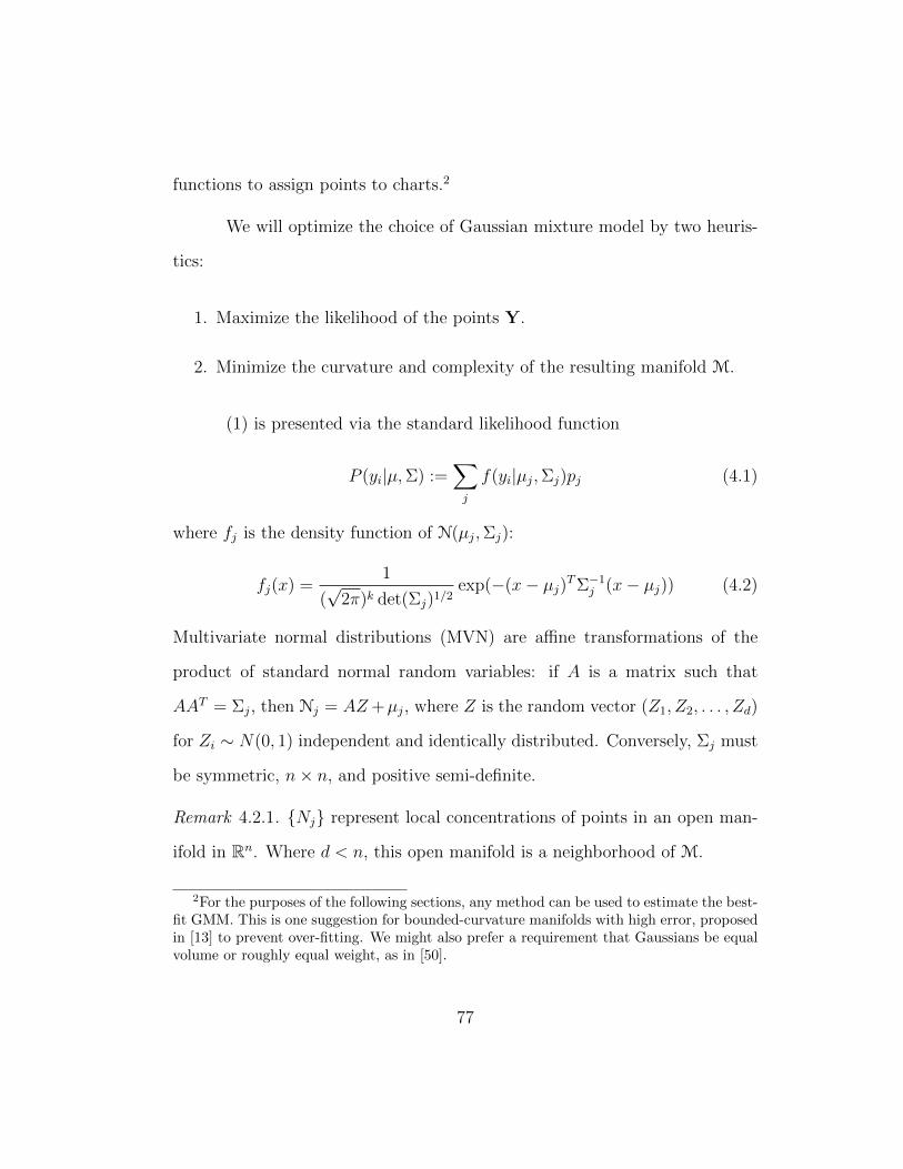
functions to assign points to charts.2

We will optimize the choice of Gaussian mixture model by two heuris-

tics:

1. Maximize the likelihood of the points Y.

2. Minimize the curvature and complexity of the resulting manifold M.

(1) is presented via the standard likelihood function

P (yi|µ,Σ) :=∑j

f(yi|µj,Σj)pj (4.1)

where fj is the density function of N(µj,Σj):

fj(x) =1

(√2π)k det(Σj)1/2

exp(−(x− µj)TΣ−1

j (x− µj)) (4.2)

Multivariate normal distributions (MVN) are affine transformations of the

product of standard normal random variables: if A is a matrix such that

AAT = Σj, then Nj = AZ+µj, where Z is the random vector (Z1, Z2, . . . , Zd)

for Zi ∼ N(0, 1) independent and identically distributed. Conversely, Σj must

be symmetric, n× n, and positive semi-definite.

Remark 4.2.1. {Nj} represent local concentrations of points in an open man-

ifold in Rn. Where d < n, this open manifold is a neighborhood of M.

2For the purposes of the following sections, any method can be used to estimate the best-fit GMM. This is one suggestion for bounded-curvature manifolds with high error, proposedin [13] to prevent over-fitting. We might also prefer a requirement that Gaussians be equalvolume or roughly equal weight, as in [50].

77

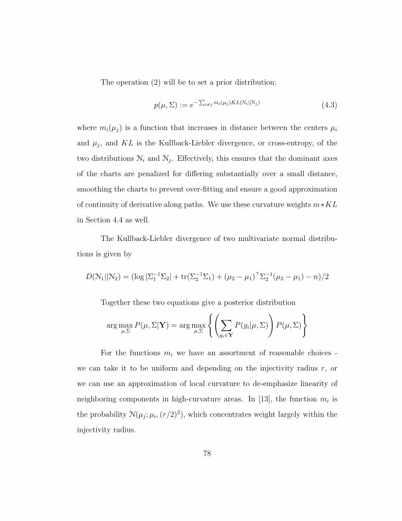
The operation (2) will be to set a prior distribution:

p(µ,Σ) := e−∑

i=j mi(µj)KL(Ni||Nj) (4.3)

where mi(µj) is a function that increases in distance between the centers µi

and µj, and KL is the Kullback-Liebler divergence, or cross-entropy, of the

two distributions Ni and Nj. Effectively, this ensures that the dominant axes

of the charts are penalized for differing substantially over a small distance,

smoothing the charts to prevent over-fitting and ensure a good approximation

of continuity of derivative along paths. We use these curvature weights m∗KL

in Section 4.4 as well.

The Kullback-Liebler divergence of two multivariate normal distribu-

tions is given by

D(N1||N2) = (log |Σ−11 Σ2|+ tr(Σ−1

2 Σ1) + (µ2 − µ1)⊤Σ−1

2 (µ2 − µ1)− n)/2

Together these two equations give a posterior distribution

argmaxµ,Σ

P (µ,Σ|Y) = argmaxµ,Σ

{(∑yi∈Y

P (yi|µ,Σ)

)P (µ,Σ)

}

For the functions mi we have an assortment of reasonable choices -

we can take it to be uniform and depending on the injectivity radius r, or

we can use an approximation of local curvature to de-emphasize linearity of

neighboring components in high-curvature areas. In [13], the function mi is

the probability N(µj;µi, (r/2)2), which concentrates weight largely within the

injectivity radius.

78

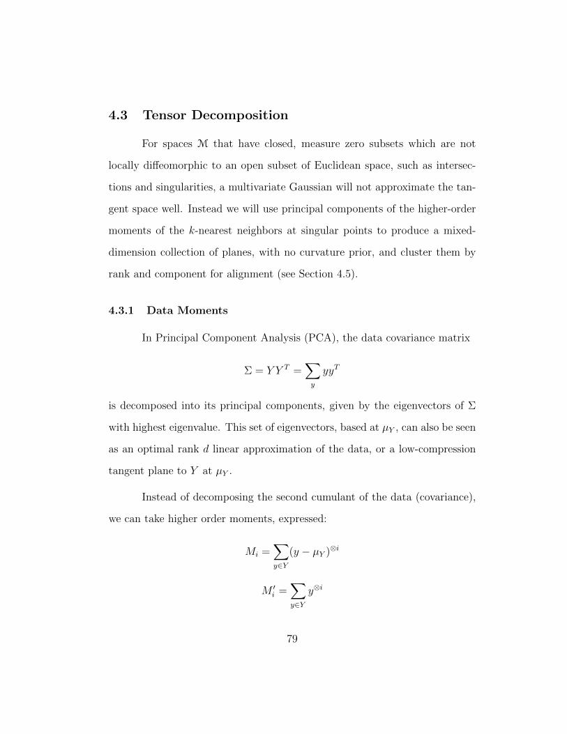
4.3 Tensor Decomposition

For spaces M that have closed, measure zero subsets which are not

locally diffeomorphic to an open subset of Euclidean space, such as intersec-

tions and singularities, a multivariate Gaussian will not approximate the tan-

gent space well. Instead we will use principal components of the higher-order

moments of the k-nearest neighbors at singular points to produce a mixed-

dimension collection of planes, with no curvature prior, and cluster them by

rank and component for alignment (see Section 4.5).

4.3.1 Data Moments

In Principal Component Analysis (PCA), the data covariance matrix

Σ = Y Y T =∑y

yyT

is decomposed into its principal components, given by the eigenvectors of Σ

with highest eigenvalue. This set of eigenvectors, based at µY , can also be seen

as an optimal rank d linear approximation of the data, or a low-compression

tangent plane to Y at µY .

Instead of decomposing the second cumulant of the data (covariance),

we can take higher order moments, expressed:

Mi =∑y∈Y

(y − µY )⊗i

M ′i =

∑y∈Y

y⊗i

79

for the centralized moment and the moment about the origin, respectively.3

This i-moment is a real symmetric tensor of order i.

Summarizing the data via its principal components works most accu-

rately for Gaussian random variables, for which the principal components are

the orthogonal directions with highest subsequent variance, and the distribu-

tion is independent along each, so that it can be completely specified by a

mean and covariance matrix. In general, higher order moments (and more

directly, cumulants) can be seen as some measure of non-Gaussian behavior

- cumulants of a multivariate normal distribution vanish after the first and

second.

4.3.2 GPCA using symmetric block decomposition

In [33], Kileel and Pereira define a symmetric block decomposition algo-

rithm using Sylvester’s catalecticant method, which factors a symmetric tensor

T into a sum of real symmetric Tucker products :

T =R∑i=1

(Ai;Ai; . . . ;Ai) · Λi

for a collection of core tensors Λi ∈ SymTmℓi, and factor matrices Ai ∈ Mn×ℓi .

This is called an (A1, . . . , AR)-symmetric block term tensor decomposition.

This is similar to other block term decompositions (see, e.g. [34][35][36]),

except the decomposition itself is symmetric.

3We note that this can be computationally intensive. Recent results of Sherman andKolda allow for implicit computation of low-rank symmetric approximations to the higher-order moment tensors[51].

80

Suppose Y ∈ Rn is a random variable supported on a subspace ar-

rangement S = ∪Ri=1Si ⊂ Rn, where each Si is a linear subspace of respective

dimension di. Then for Ai ∈ Mn×di such that Si = colspan(Ai), for each m,

the moment tensor E[Y ⊗m] ∈ SymTmn admits a symmetric block term decom-

position as above, with Ai as factor matrix coefficients. This is Lemma 6.1 in

[33]; we replicate the proof here to give demonstrate the particular significance

of the decomposition.

Proof. First, we decompose Y . Let x be the discrete random variable over

[R] with probabilities wi corresponding to the measure of Y restricted to the

subspace Si. For a choice of basis b1, . . . , bdi of Si, let Bi be the n× di matrix

(b1b2 . . . bdi)T . Let yi be the random variable in Rdi induced by the projection

Bi : Si → Rdi . Then Y = {Biyi}x, and

E[Y ⊗m] =R∑i=1

wiE[(Biyi)⊗m] (4.4)

Multilinearity of the m-way tensor product and linearity of expectation give

=R∑i=1

wi(Bi; . . . ;Bi) · E[y⊗mi ]. (4.5)

Setting Λi = wiE[y⊗mi ], we see that this decomposes the m-moment of Y from

an m-tensor of length n to a sum of R m-tensors of respective length di, each

corresponding to the n-moment of the restriction of Y to Si using a particular

choice of basis.

Of course, the choice of basis for a subspace Si is only unique up to ac-

tion of GLd(R). As for the converse - if we decompose the moment tensor into

81

symmetric blocks, is Y supported minimally on that subspace arrangement?

- computational convergence may depend on properties of the arrangement,

such as the dimension of pairwise intersections.

4.3.3 Local rank estimation

The naive approach to adapting [63], [49] to the stratified or trans-

versely intersecting setting would be to apply GPCA to k-nearest neighbors

at each point. This is possible, but since GPCA detects linear subspace ar-

rangements, and not affine subspace arrangements, the results we get a small

distance from an intersection locus will not reflect the local structure accu-

rately.

A better method would be to detect points x at which the tangent

space is a union of linear subspaces based at x in Rn. To accomplish this,

we assume we have a uniform sampling density ρ, and examine the growth of

neighborhoods based at x.

Let βx(r) be the number of points y ∈ Y such that ||y − x|| ≤ r. Then

for a d-dimensional locally linear neighborhood, under ideal circumstances,

βx(r) = ρAdrd

where Ad is the volume of a unit ball in Rd, and

(log(βx(r)))′ =

d

r,

so that the dimension is approximately the slope of the plot log(βx(r)). In

practice, these values are computed with βx(r) as the independent variable:

82

ordering nearest neighbors by distance, βx(r) takes on discrete values 1, 2, . . . , k

(if we are using the k nearest neighbors), and the radius of each new point is

recorded. We can average the slope by computing

1

log(k)

k∑i=1

log(i)− log(i− 1)

ri − ri−1

· ri

However, at small scales, noise will cause βx(r) to grow as ρAnrn, and as r

exceeds the injectivity radius, reach, or nears the radius of curvature in any

direction, βx(r) will grow in excess of d again. If we have bounds on curvature,

reach, injectivity, and noise, then we can take the sum

1

log(max{i : ri < κ}/min{i : ri > ϵ})∑

i:ϵ<ri<κ

rilog(i)− log(i− 1)

ri − ri−1

for only those neighbors in the annulus ϵ < r < κ, for ϵ the upper bound

on noise and κ the lower bound on reach, injectivity, and curvature in any

direction, to increase accuracy.

If x is on the singular locus of M, contained in the closure of a d-

dimensional stratum, then the growth will look similar:

βx(r) = mxρAdrd

where mx can be an integer, if Tx(M) is a union of mx linear subspaces; or

a multiple of 1/2, if x lies on the boundary of a halfspace; or another real

number if x is a cone-type singularity.

Given d, to estimate mx we compute the values

βx(r)

ρAdrd

83

for all r. We suspect this can be used to give a rank estimate for the local

moment tensor∑

y∈kNN(x) y⊗i, given some restrictions on the singularity type.

If x is a singular point lying in the closure of a number of strata of

different dimensions di, then

r log(βx(r))′ =

∑dimx,iAdir

di∑mx,iAdir

di

will not be linear, but it will be continuous - this distinguishes it from the case

where Tx can’t be estimated accurately by tensor decomposition; if x is near a

singular point, or the neighborhood radius exceeds the reach, then log(βx(r))′

will be discontinuous, and we should not use this neighborhood for tangent

plane inference.

4.4 Multiple charts

Let {µi,Σi} be a Gaussian mixture fit to the data Y . Associated to

this mixture are the density functions fi(y) (See 4.2). For (i1, . . . , iℓ) ∈ [k]ℓ,

define the probability vector

q(i1,...,iℓ)(y) = min(fi1(y), fi2(y), . . . , fiℓ(y))

We choose a threshold value t for the nerve complex. A reasonable value

of t will depend on the ambient dimension and the size of M, such as t ∼

(2π)−n/2|Y |−1/2 where |Y | is the volume of the convex hull of points Y .

Definition 4.4.1. We define the nerve complex ∆t(Y, {µi,Σi}) for t ∈ [0, 1]:

• ∆0 = [k], for k the number of charts

84

• For ℓ ≥ 2, (i1, . . . , iℓ) ∈ ∆(Y )ℓ when ||q(i1,...,iℓ)||∞ > t.

For M a stratified manifold or union of manifolds, we may want to

add the pairwise Kullback-Leibler divergence of (i1, . . . , iℓ) into q(i1,...,iℓ), so

that transverse tangent spaces are less likely to be highly connected. For

M a Riemannian manifold, we can relax restrictions on curvature by using

intersection for adjacency.

Definition 4.4.2. ∆(Y, {µi,Σi}) is called flag if for every v1, . . . , vℓ, vℓ+1 ∈

V (∆(Y )) such that (vi, vj) ∈ E(∆(Y )) for all i = j ∈ [ℓ+1], then (v1 . . . vℓ+1) ∈

∆ℓ is an ℓ-simplex in ∆ (see 2.2.1).

If ∆(Y ) is flag, then by definition, it can be stored by its graph adja-

cency matrix.

Lemma 4.4.1. ∆(Y ) is a flag simplicial complex, i.e. σ′ ⊂ σ implies σ′ ∈

∆(Y ) for every σ ∈ ∆(Y ), and if σ ∈ ∆(Y ) for every face σ of σ′, then

σ′ ∈ ∆(Y ).

Proof. That ∆(Y ) is a simplicial complex follows from the fact that

min(fi1 , . . . , fiℓ , fiℓ+1) ≤ min(fi1 , . . . , fiℓ),

so that if the former is greater than t for some y, and therefore a simplex in

∆(Y ), using the same y, its faces are as well.

To show that ∆(Y ) is flag, suppose maxy(q(j,k)(y)) > t for all j, k ∈

(i1, . . . , iℓ). Then

maxy

(q(i1,...,iℓ)(y)) = maxy

(mini

fi(y)) = maxy

(mini,j

q(i,j)(y)) > t

85

shows that (i1, . . . , iℓ) is the basis of a simplex in ∆(Y ).

The nerve complex represents the nerve of the open cover (Ui, [Vi]d)

of Y (the projection to the principal components of Σi, see Section 4.5.1), a

discrete approximation of M, where M is compact. We are inspired by the

Nerve Theorem:

Theorem 4.4.1. (Nerve Theorem, see Hatcher [29]) If X is a paracompact

space, and U is an open cover of X such that the intersection of any finite

subfamily of U is either empty or contractible, then |∆(U)| ≃ X, i.e. the

geometric realization of ∆(U) is homotopy equivalent to X.

Assuming that U is a Cech cover of M, the nerve preserves the homo-

topy type of M. Using operations which preserve the topology of |∆(U)|, we

construct a simpler complex which contains instructions for the combination

of multiple tangent planes into charts.

The main technique we will use is edge contraction. In [20], it is proven

that if the edge ab satisfies a link condition in the complex ∆, then the contrac-

tion ∆/C(a, b) ≃ ∆. Regarding the charts, contraction will mean combining

the charts Ua and Ub, or if a and b already represent index sets A and B,

then contraction will result in a vertex label A ∪ B, so that all charts Ui for

i ∈ A ∪B are aligned using Section 4.5.1.

Definition 4.4.3. (See 1.1.3 for comparison; this is slightly more general) The

star of a set X ⊂ ∆ denoted St(X), is the set of cofaces of all σ ∈ X, that

86

is, all simplices containing σ as a face. For a subset S of ∆, the closure of S,

denoted S, is the set of simplices in S and all of their faces. Then the link of

X, denoted Lk(X), is the set of simplices in St(X) \ St(X).

The link condition for an edge ab is satisfied if Lk(ab) = Lk(a)∩Lk(b).

To check this, we must be able to compute the link: find all simplices σ

containing a (resp. b, ab), list all faces, and use set operations to compare

Lk(ab) with Lk(a) and Lk(b).

Lemma 4.4.2. If ∆ is a flag complex, the link condition can be checked using

the adjacency matrix, without constructing higher simplices.

Proof. We first show that if v is a 0-simplex, then Lk(v) = Lk(v) can be

computed using adjacencies. Let w1, . . . , wm be the set of neighbors of v,

and find {e ∈ ∆ : e = (wi, wj)}. Then the link of v is given by the flag

complex over w1, . . . , wm, {e = (wi, wj)}: since v is adjacent to all wi, if a

set of wi1 , wi2 , . . . , wik are pairwise adjacent, then since ∆ is a flag complex,

< wi1 , wi2 , . . . , wik > is a face of the simplex < v,wi1 , wi2 , . . . , wik > in δ. For

a 1-simplex e = (v, w), Lk(e) is given by the flag complex over the induced

subgraph on N(v) ∩N(w). So the link condition can be checked by comput-

ing the neighbor sets N(v) and N(w), taking the intersection N(v) ∩ N(w),

finding the induced subgraph ∆N(v),∆N(w),∆N(v,w) for each, and comparing

the intersection ∆N(v) ∩∆N(w) with ∆N(v,w).

87

4.4.1 Procedure

Once we have our nerve complex ∆, we search for a cover of ∆ via

contractible subcomplexes, favoring neighbors which are closer in mean and

tangent space spanned.

1. For each e = (v, w) ∈ E(∆), let Fvw = e−|mv(µw)+mw(µv)|∗KL(Nv ||Nw), for m

as in Section 4.2 and KL the Kullback-Liebler divergence of Gaussian

distributions Nb and Nv.

2. Begin with a random basepoint b ∈ V (∆).

3. For all edges (b, v) incident to b, check the link condition. Denote by Eb

the set of edges satisfying the link condition.

4. Choose v = argminv Fbv.

5. Contract edge (b, v): for each simplex containing v, map σ = (. . . , v, . . . ) 7→

(. . . , b, . . . ). When a simplex contains both b and v, it collapses down

one dimension. Relabel b as b∪v. If σ is a 1-simplex (edge), it retains its

value Fvw, except when σ is produced by the contraction of a 2-simplex

to a 1-simplex; in that case, F(b∪v)w := min(Fbw, Fvw).

6. At the i-th iteration, basepoint bI now has labels b, v1, . . . , vi−1. Again,

we check the link condition for all neighbors, choose the neighbor vi =

argminFbIv, and contract.

88

7. Stop when |I| ≥ maxsize, or when no incident edges satisfy the link

condition.

8. Repeat the process, choosing a new basepoint when necessary, until no

edges satisfy the link condition. The number of vertices in the final

complex is the chart number C, and the set of vertex labels is the nerve

cover I1, . . . , IC .

9. Once we have the nerve cover {I1, . . . , IC}, we pass each index set I to

the flat alignment algorithm of Section 4.5.1: create the submatrix of

QQT (as in 4.5.1) with rows and columns indexed by I, take the trailing

eigenvectors of QIQTI + 1 to get GI , which maps the sets Uj for j ∈ I to

a common chart in Rd.

10. The result is C charts, with transition maps as defined in Section 4.4.2.

89

Algorithm 3 Nerve Decomposition Algorithm

1: for (v, w) ∈ ∆1, compute Fvw from {µi,Σi} values.2: points = random ordering of ∆0

3: for b ∈ points:4: set I[b] = {b}.5: while(|I[b]| ≤maxsize):6: Find neighb = {(b, v) ∈ ∆1}7: for (b, v) ∈ neighb:8: If link condition(b, v) = true and v not in I already:9: add (b, v) to Eb

10: if Eb = NULL: break11: else:12: find argument (b, v∗) of min{Fbv : (b, v) ∈ Eb}.13: (∆, F ) = contract(∆, F, (b, v∗)))14: add v∗ to I[b].15: remove v∗ from points

16: C = length(I)17: return (∆, I)

Since we are adding vertices by adjacency, UI always remains connected. Sim-

ilarly, UI is contractible, since by results of [20], I is produced by topology-

preserving contraction of the nerve complex. The homotopy type of the tan-

gent space cover {Ui} is given by the type of the resulting contracted nerve.

The number of charts C is bounded below by the topological complexity of

the cover Ui, which approximates TC(M).

For k <√N , the alignment step dominates runtime, but efficiencies

can be obtained in reducing the storage of ∆.

90

4.4.2 Transition Maps

There are a couple distinct natural ways to define the transition maps

ϕ′ij : U

′i → U ′

j.

By linear alignment: for each pair U ′i and U ′

j of new charts, if their

intersection on Y is non-empty (with respect to the threshold), there is a subset

vi ∈ U ′i and wj ∈ U ′

j such that vi is contained in a simplex that intersects U ′j,

and similarly with wj. Then the transition maps are defined on connected

components of vi ∪ wj by the linear alignment GC(vi∪wj).

By interpolation of data: U ′i → U ′

j for U ′i ∩ U ′

j = ∅ are given on Y by

the image of y in each - if pyi′ > t, pyj′ > t, then ϕij(GU ′iy) = GU ′

j(y). This

map will not be linear, continuous, or well-defined on points not in Y , but it

will provide the best preservation of paths in Y .

4.4.3 Intersection Spaces

Suppose we have a local decomposition of tensors as given in Section

4.3.2, i.e. a collection of R weights wi, projection matrices Bi, and moment

tensors Λi.

If∑

(Bi;Bi;Bi;Bi)Λi is a 4th moment, and if a neighborhood of the

singular point x at which GPCA has been performed looks like a mixture of

Gaussians based at x and supported on the subspaces generated by Bi, then

Wick’s Theorem implies that on each subspace,

E[(yi − µi)⊗4]ijkℓ = ΣijΣkℓ + ΣikΣjℓ + ΣiℓΣjk

91

so that the covariance matrix entries generate the fourth moment, and with

enough information, can be recovered. In [23], a technique is described to give

a maximum likelihood mixture of mean-zero Gaussians using tensor decom-

position of the 3rd, 4th, and 6th moments. We propose either an analogous

technique, or to use a direct tangent space alignment such as [63] which does

not depend on a maximum variance basis for the tangent plane.

Once we have a collection of transverse Gaussians centered at µ, we can

alternately depend on the high Kullback-Liebler divergence between different

subspaces to prevent adjacency in the nerve complex, adjust mµ(µ) to be

quite large, or manually enforce that Gaussians based at the same mean are

an independent set in the complex. This will allow Algorithm 3 to separate

the charts into different components.

4.4.4 Nerve Conjectures

Conjecture 1. Let M ⊂ Rn be a smooth manifold, with reach ρ and curvature

bounded by κ. Let ϵ < ρ/2 be given. Suppose Y is a random uniform sample

of sufficiently high density. If the nerve ∆(Y, {µi,Σi}) is contractible and k

sufficiently large, then P(M ≃ ·) → 1.

Conjecture 2. Let M be a manifold in Rn, and let {Ui} ⊂ M be a Cech cover

of open balls of radius r, with r less than the reach and injectivity radius.

Replace each Ui with a Gaussian distribution centered at p with axes in the

tangent plane to p of length r, and normal axes of length ϵ. Let Y ∼ Unif(Mϵ)

be a sample of size N . Then P[∆(Y, {µi,Σi}) ≃ M] → 1 as N → ∞.

92

4.5 The alignment G

Once we have the model best fitting the data, we can take advantage

of the intrinsic dimension d of the data to compute a dimensionality reduction

map which reflects the local geometry. If M, or a suitable subset of M, is

contractible and close to flat, then we will be able to assemble the local charts

linearly into a best-fit map to Rd.

4.5.1 Flat alignment of Gaussians

Here we follow a technique similar to [13] or [63], with some modifica-

tions as noted.

N number of data points in Yn original dimension, y ∈ Rn

d intrinsic dimensionD ambient dimension of desired embedding, D ≥ d

Let D ≥ d be the chosen ambient embedding dimension for our align-

ment. A smaller D produces more data compression; D = d produces a classic

tangent space alignment. An ambient codimension of 1 or 2 may be desired

to preserve intrinsic features of M, for example if M is not contractible or has

high curvature, keeping in mind that in some cases, M might not isometrically

embed without an ambient dimension over 2d.

Per Section 4.2, we have a set {(µk,Σk)} of multivariate Gaussians

with global weight vector wk. Using the corresponding density functions f ,

this gives rise to pointwise assignment weights wky = fµk,Σk(y) ∗ wk of each

93

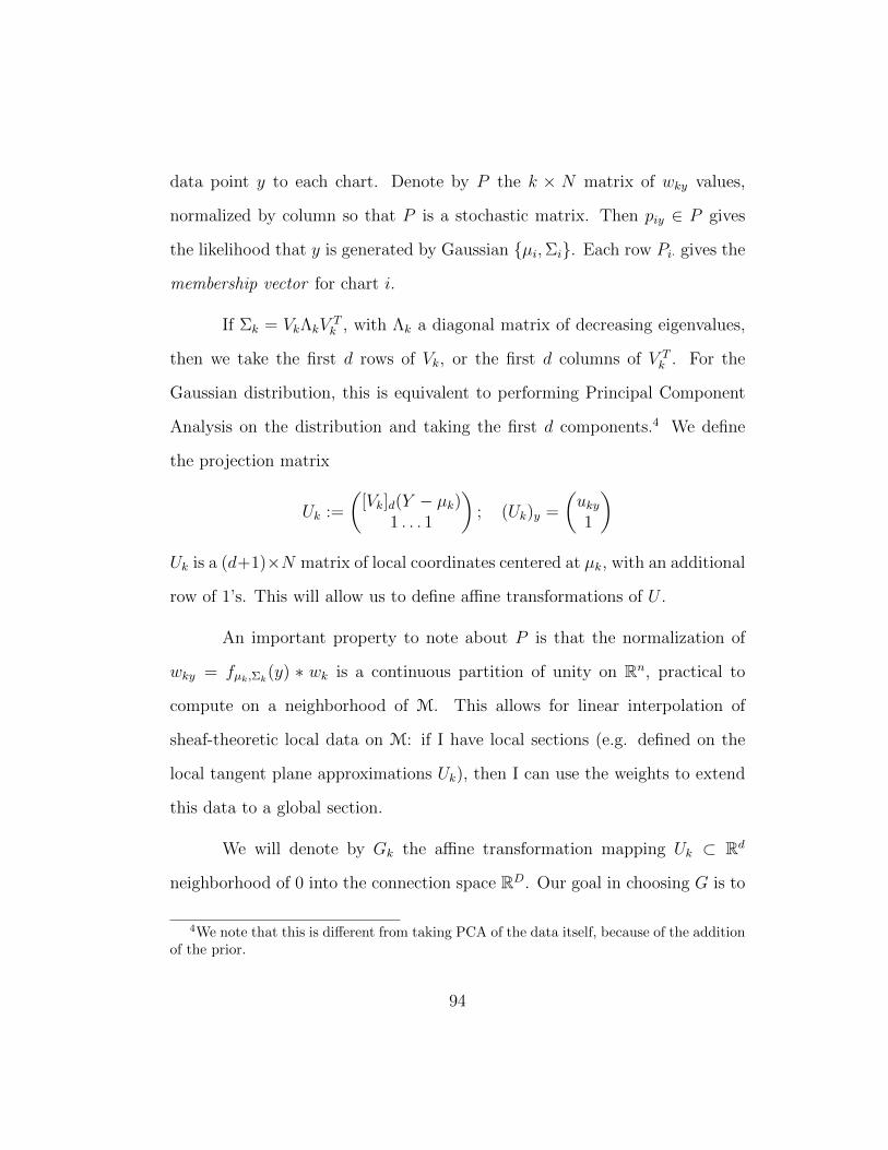
data point y to each chart. Denote by P the k × N matrix of wky values,

normalized by column so that P is a stochastic matrix. Then piy ∈ P gives

the likelihood that y is generated by Gaussian {µi,Σi}. Each row Pi· gives the

membership vector for chart i.

If Σk = VkΛkVTk , with Λk a diagonal matrix of decreasing eigenvalues,

then we take the first d rows of Vk, or the first d columns of V Tk . For the

Gaussian distribution, this is equivalent to performing Principal Component

Analysis on the distribution and taking the first d components.4 We define

the projection matrix

Uk :=

([Vk]d(Y − µk)

1 . . . 1

); (Uk)y =

(uky

1

)Uk is a (d+1)×N matrix of local coordinates centered at µk, with an additional

row of 1’s. This will allow us to define affine transformations of U .

An important property to note about P is that the normalization of

wky = fµk,Σk(y) ∗ wk is a continuous partition of unity on Rn, practical to

compute on a neighborhood of M. This allows for linear interpolation of

sheaf-theoretic local data on M: if I have local sections (e.g. defined on the

local tangent plane approximations Uk), then I can use the weights to extend

this data to a global section.

We will denote by Gk the affine transformation mapping Uk ⊂ Rd

neighborhood of 0 into the connection space RD. Our goal in choosing G is to

4We note that this is different from taking PCA of the data itself, because of the additionof the prior.

94

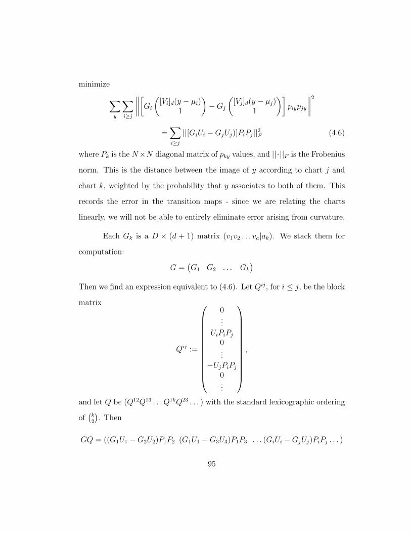
minimize∑y

∑i≥j

∥∥∥∥[Gi

([Vi]d(y − µi)

1

)−Gj

([Vj]d(y − µj)

1

)]piypjy

∥∥∥∥2=∑i≥j

||[GiUi −GjUj)]PiPj||2F (4.6)

where Pk is the N×N diagonal matrix of pky values, and ||·||F is the Frobenius

norm. This is the distance between the image of y according to chart j and

chart k, weighted by the probability that y associates to both of them. This

records the error in the transition maps - since we are relating the charts

linearly, we will not be able to entirely eliminate error arising from curvature.

Each Gk is a D × (d + 1) matrix (v1v2 . . . va|ak). We stack them for

computation:

G =(G1 G2 . . . Gk

)Then we find an expression equivalent to (4.6). Let Qij, for i ≤ j, be the block

matrix

Qij :=

0...

UiPiPj

0...

−UjPiPj

0...

,

and let Q be (Q12Q13 . . . Q1kQ23 . . . ) with the standard lexicographic ordering

of(k2

). Then

GQ = ((G1U1 −G2U2)P1P2 (G1U1 −G3U3)P1P3 . . . (GiUi −GjUj)PiPj . . . )

95

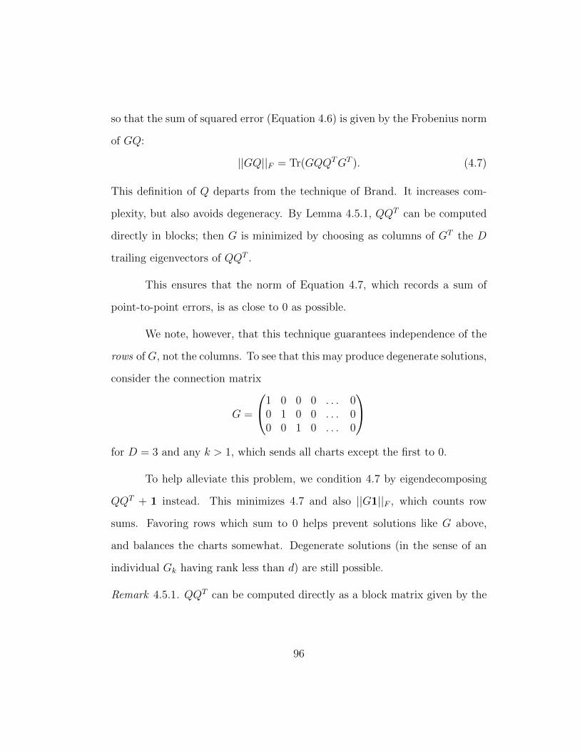
so that the sum of squared error (Equation 4.6) is given by the Frobenius norm

of GQ:

||GQ||F = Tr(GQQTGT ). (4.7)

This definition of Q departs from the technique of Brand. It increases com-

plexity, but also avoids degeneracy. By Lemma 4.5.1, QQT can be computed

directly in blocks; then G is minimized by choosing as columns of GT the D

trailing eigenvectors of QQT .

This ensures that the norm of Equation 4.7, which records a sum of

point-to-point errors, is as close to 0 as possible.

We note, however, that this technique guarantees independence of the

rows of G, not the columns. To see that this may produce degenerate solutions,

consider the connection matrix

G =

1 0 0 0 . . . 00 1 0 0 . . . 00 0 1 0 . . . 0

for D = 3 and any k > 1, which sends all charts except the first to 0.

To help alleviate this problem, we condition 4.7 by eigendecomposing

QQT + 1 instead. This minimizes 4.7 and also ||G1||F , which counts row

sums. Favoring rows which sum to 0 helps prevent solutions like G above,

and balances the charts somewhat. Degenerate solutions (in the sense of an

individual Gk having rank less than d) are still possible.

Remark 4.5.1. QQT can be computed directly as a block matrix given by the

96

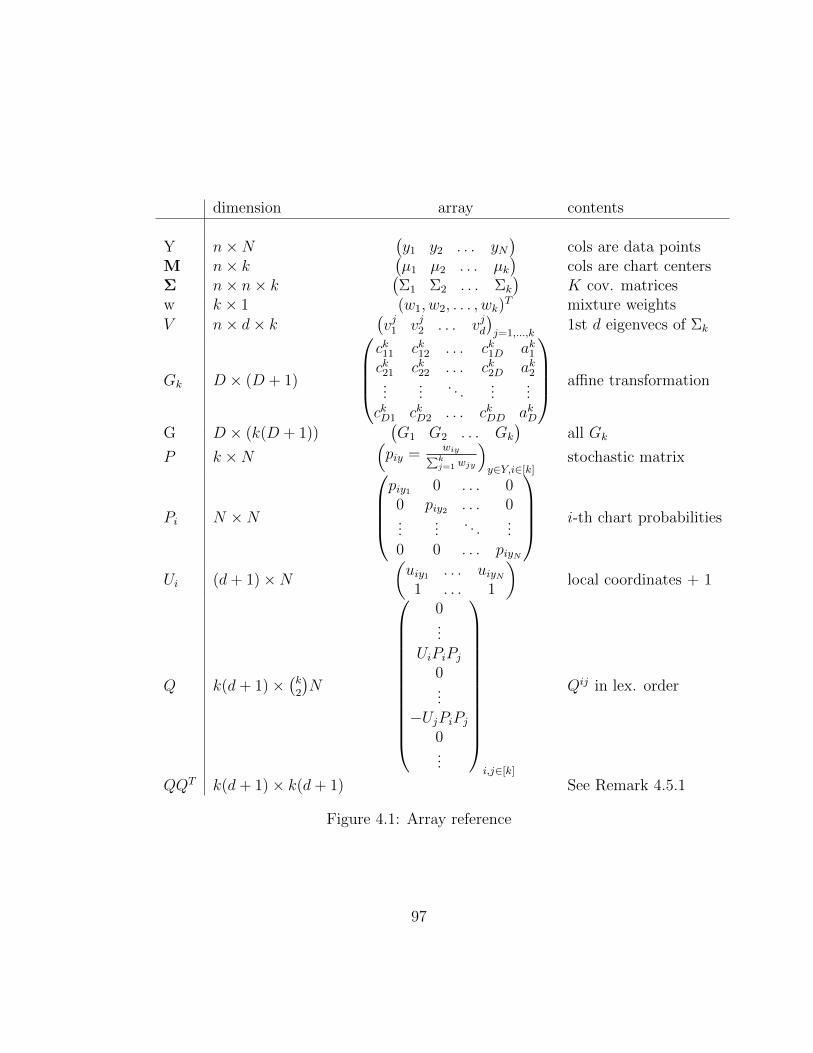
dimension array contents

Y n×N(y1 y2 . . . yN

)cols are data points

M n× k(µ1 µ2 . . . µk

)cols are chart centers

Σ n× n× k(Σ1 Σ2 . . . Σk

)K cov. matrices

w k × 1 (w1, w2, . . . , wk)T mixture weights

V n× d× k(vj1 vj2 . . . vjd

)j=1,...,k

1st d eigenvecs of Σk

Gk D × (D + 1)

ck11 ck12 . . . ck1D ak1ck21 ck22 . . . ck2D ak2...

.... . .

......

ckD1 ckD2 . . . ckDD akD

affine transformation

G D × (k(D + 1))(G1 G2 . . . Gk

)all Gk

P k ×N(piy =

wiy∑kj=1 wjy

)y∈Y,i∈[k]

stochastic matrix

Pi N ×N

piy1 0 . . . 00 piy2 . . . 0...

.... . .

...0 0 . . . piyN

i-th chart probabilities

Ui (d+ 1)×N

(uiy1 . . . uiyN

1 . . . 1

)local coordinates + 1

Q k(d+ 1)×(k2

)N

0...

UiPiPj

0...

−UjPiPj

0...

i,j∈[k]

Qij in lex. order

QQT k(d+ 1)× k(d+ 1) See Remark 4.5.1

Figure 4.1: Array reference

97

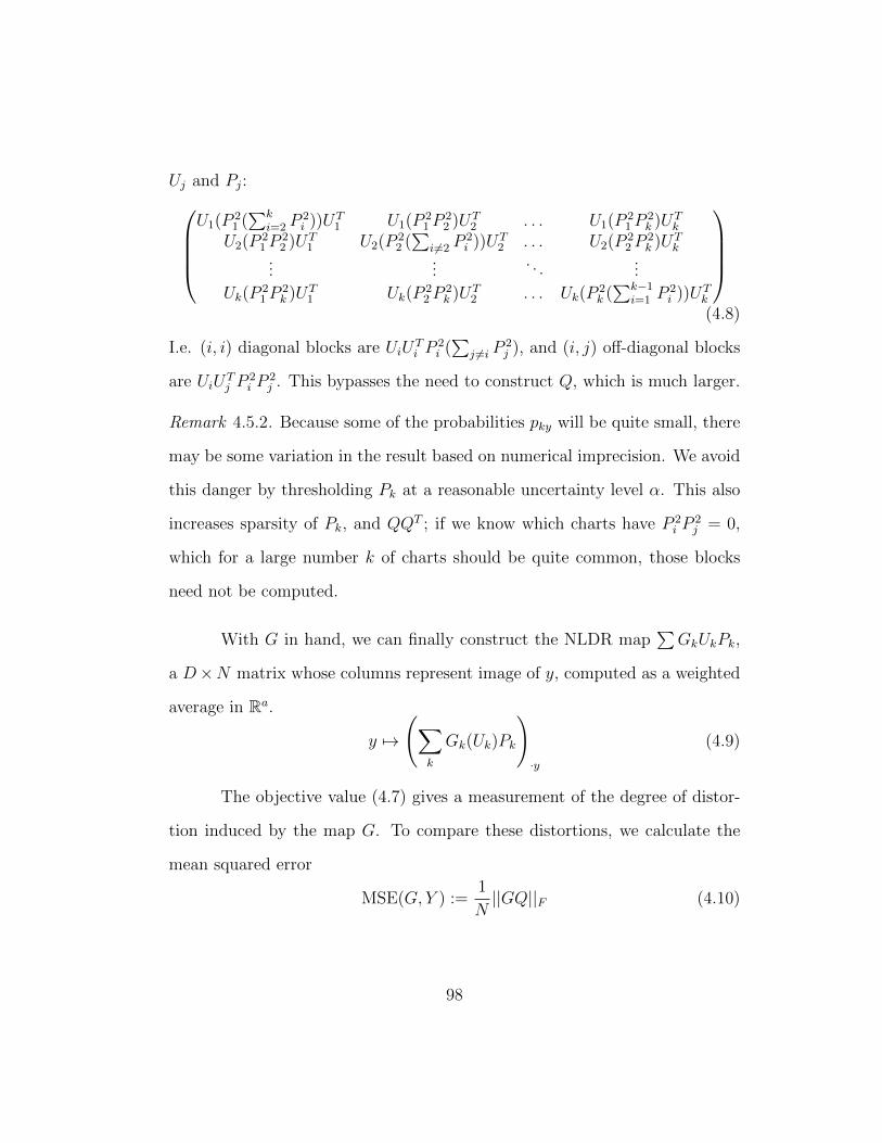
Uj and Pj:U1(P

21 (∑k

i=2 P2i ))U

T1 U1(P

21P

22 )U

T2 . . . U1(P

21P

2k )U

Tk

U2(P21P

22 )U

T1 U2(P

22 (∑

i =2 P2i ))U

T2 . . . U2(P

22P

2k )U

Tk

......

. . ....

Uk(P21P

2k )U

T1 Uk(P

22P

2k )U

T2 . . . Uk(P

2k (∑k−1

i=1 P2i ))U

Tk

(4.8)

I.e. (i, i) diagonal blocks are UiUTi P

2i (∑

j =i P2j ), and (i, j) off-diagonal blocks

are UiUTj P

2i P

2j . This bypasses the need to construct Q, which is much larger.

Remark 4.5.2. Because some of the probabilities pky will be quite small, there

may be some variation in the result based on numerical imprecision. We avoid

this danger by thresholding Pk at a reasonable uncertainty level α. This also

increases sparsity of Pk, and QQT ; if we know which charts have P 2i P

2j = 0,

which for a large number k of charts should be quite common, those blocks

need not be computed.

With G in hand, we can finally construct the NLDR map∑

GkUkPk,

a D×N matrix whose columns represent image of y, computed as a weighted

average in Ra.

y 7→

(∑k

Gk(Uk)Pk

)·y

(4.9)

The objective value (4.7) gives a measurement of the degree of distor-

tion induced by the map G. To compare these distortions, we calculate the

mean squared error

MSE(G, Y ) :=1

N||GQ||F (4.10)

98

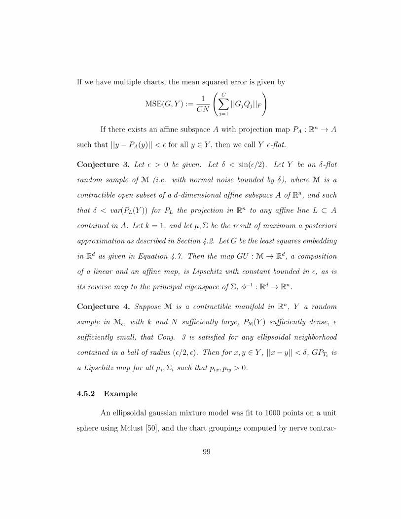
If we have multiple charts, the mean squared error is given by

MSE(G, Y ) :=1

CN

(C∑

j=1

||GjQj||F

)

If there exists an affine subspace A with projection map PA : Rn → A

such that ||y − PA(y)|| < ϵ for all y ∈ Y , then we call Y ϵ-flat.

Conjecture 3. Let ϵ > 0 be given. Let δ < sin(ϵ/2). Let Y be an δ-flat

random sample of M (i.e. with normal noise bounded by δ), where M is a

contractible open subset of a d-dimensional affine subspace A of Rn, and such

that δ < var(PL(Y )) for PL the projection in Rn to any affine line L ⊂ A

contained in A. Let k = 1, and let µ,Σ be the result of maximum a posteriori

approximation as described in Section 4.2. Let G be the least squares embedding

in Rd as given in Equation 4.7. Then the map GU : M → Rd, a composition

of a linear and an affine map, is Lipschitz with constant bounded in ϵ, as is

its reverse map to the principal eigenspace of Σ, ϕ−1 : Rd → Rn.

Conjecture 4. Suppose M is a contractible manifold in Rn, Y a random

sample in Mϵ, with k and N sufficiently large, PM(Y ) sufficiently dense, ϵ

sufficiently small, that Conj. 3 is satisfied for any ellipsoidal neighborhood

contained in a ball of radius (ϵ/2, ϵ). Then for x, y ∈ Y , ||x− y|| < δ, GPTiis

a Lipschitz map for all µi,Σi such that pix, piy > 0.

4.5.2 Example

An ellipsoidal gaussian mixture model was fit to 1000 points on a unit

sphere using Mclust [50], and the chart groupings computed by nerve contrac-

99

tion as in Section 4.4. The output contracted nerve is the boundary of a 3-

simplex (homeomorphic to the sphere), with basis {(4), (2, 6, 8, 10), (7), (1, 3, 5, 9)}.

The grouped charts were then aligned using Section 4.5.1, and plotted accord-

ing to Equation 4.9, with size of point given by the probability it belongs to

that chart collection. The resulting visualization in R2 is given in Figure 4.2.

Figure 4.2: Left, 1000 points on a sphere in R3. Right, the visualized charts.

4.5.3 Spherical Alignment

If M is not contractible, then it will not embed diffeomorphically in Rd;

however, we may have a reasonable embedding in Rd+1 or Rd+2.

Here we restrict to the special case where D = d+1, and we would like

to fit the data to the unit sphere Sd.

100

We modify the technique of the previous section, adding constraints to

the optimization problem (4.7).

||ai|| = 1, ⟨cij, ai⟩ = 0 (4.11)

for cij columns of Gi. This ensures that the center of the tangent plane is

translated to a point on Sd, and that span(ci1, ci2, . . . , c

id) lies in TSd(ai) ⊂ Rd+1.

Let λ be a vector of Lagrange multipliers

(λ11, λ

12, . . . , λ

1d, λ

1d+1, λ

21, λ

22, . . . , λ

2d, λ

2d+1, . . . , . . . , λ

k1, λ

k2, . . . , λ

kd, λ

kd+1)

T

where λij corresponds to the j-th column vector of Gi via the equations

L(λ,G) = Tr(GQQTGT )−∑

λij⟨cij, ai⟩

0 = ∇GTr(GQQTGT )−∑

λij∇G⟨cij, ai⟩

0 = 2GQQT −d∑

j=1

∑i

λij

(. . . 0 ai . . . cij 0 . . .

)+∑i

λid+1

(0 . . . 0 2ai . . . 0

)0 = 2GQQT −GΛ,

where Λ is the matrix

Λ =

B1 0 . . . 00 B2 . . . 0...

.... . .

...0 0 . . . Bk

; Bi =

0 . . . 0 λi

1

0 . . . 0 λi2

.... . .

......

0 . . . 0 λid

λi1 . . . λi

d 2λid+1

So we have G(2QQT − Λ) = 0, which together with the constraints ⟨cij, ai⟩ =

0, ⟨ai, ai⟩ = 1, makes (d+ 1)(d+ 2)k equations in (d+ 1)(d+ 2)k variables.

101

Index

Abstract, vi

Acknowledgments, v

BHV, 5

Bibliography, 111

chart number, 89

charts, 89, 93, 98, 99

connection cluster, 41

connection, flat, 93

core tensors, 80

Data manifolds, 72

data moments, 79

Dedication, iv

dimension estimation, 82

factor matrix, 80

flag, 12, 85

Gaussian mixture model, 77

GPCA, 79, 80

Isometries of phylogenetic tree space,

7

link, 6, 87

link condition, 87

link skeleton L1L, 29

mean squared error, 98

membership vector, 94

nerve, 76, 84, 86

nerve complex, 84

nerve cover, 89

nerve decomposition, 90

Non-contractible manifolds, 84

partition of unity, 94

PCA, 80

phylogenetic tree, 2

rank, 82

Representations of Partial Leaf Sets,

23

spherical alignment, 100

splits P, P c, 3

star, 86

tangent space alignment, 93

tensor, 80

tensor decomposition, 79, 80

transition maps, 91

tree dimensionality reduction, 25, 29–

32, 47, 48

tree space TL, 28

tree space metric, 29

tree topology, 3

tucker product, 80

102

Bibliography

[1] Alex Abreu and Marco Pacini. The automorphism group of Mtrop0,n and

Mtrop0,n . Journal of Combinatorial Theory, Series A, 154:583–597, 2018.

[2] W. A. Akanni, M. Wilkinson, C. J. Creevey, P. G. Foster, and D. Pisani.

Implementing and testing bayesian and maximum-likelihood supertree

methods in phylogenetics. Royal Society Open Science, 2(8), 08.

[3] David Ayala, John Francis, and Hiro Lee Tanaka. Local structures on

stratified spaces. Advances in Mathematics, 307:903–1028, 2017.

[4] Martin Azizyan, Aarti Singh, and Larry Wasserman. Minimax theory

for high-dimensional gaussian mixtures with sparse mean separation. In

Proceedings of the 26th International Conference on Neural Information

Processing Systems - Volume 2, NIPS’13, page 2139–2147, Red Hook,

NY, USA, 2013. Curran Associates Inc.

[5] Dennis Barden and Huiling Le. The logarithm map, its limits and frechet

means in orthant spaces. Proceedings of the London Mathematical

Society, 117(4):751–789, jun 2018.

[6] Dennis Barden, Huiling Le, and Megan Owen. Central limit theorems

for Frechet means in the space of phylogenetic trees. Electronic Journal

of Probability, 18(none):1 – 25, 2013.

103

[7] M. Bacak. Computing medians and means in Hadamard spaces. SIAM

Journal on Optimization, 24:1542–1566, 09 2014.

[8] P. Benner, M. Bacak, and P. Y. Bourguignon. Point estimates in phylo-

genetic reconstructions. Bioinformatics, 30:i534–i540, 08 2014.

[9] Louis J. Billera, Susan P. Holmes, and Karen Vogtmann. Geometry of the

space of phylogenetic trees. Advances in Applied Mathematics, 27(4):733

– 767, 2001.

[10] O. R. Bininda-Emonds, editor. Phylogenetic supertrees: combining

information to reveal the tree of life, volume 4 of Computational Biology.

Springer Netherlands, 2004.

[11] Andrew J. Blumberg, Prithwish Bhaumik, and Stephen G. Walker. Test-

ing to distinguish measures on metric spaces, 2018.

[12] Debra Boutin. Identifying graph automorphisms using determining sets.

Electr. J. Comb., 13, 09 2006.

[13] M. Brand. Charting a manifold. In NIPS, 2002.

[14] Corey Bregman. Isometry groups of cat(0) cube complexes, 2017.

[15] Daniel G. Brown and Megan Owen. Mean and Variance of Phylogenetic

Trees. Systematic Biology, 69(1):139–154, 06 2019.

104

[16] Peter Buneman. The recovery of trees from measures of dissimilarity. In

Mathematics the the Archeological and Historical Sciences, pages 387–

395, United Kingdom, 1971. Edinburgh University Press.

[17] Dmitri Burago, Yuri Burago, and Sergei Ivanov. A Course in Metric

Geometry, volume 33 of Graduate Studies in Mathematics. American

Mathematical Society, 2001.

[18] Jose Caceres, Delia Garijo, Antonio Gonzalez, Alberto Marquez, and

Marıa Puertas. The determining number of kneser graphs. Discrete

Mathematics and Theoretical Computer Science. DMTCS [electronic

only], 15, 01 2013.

[19] Damien M. de Vienne, Sebastien Ollier, and Gabriela Aguileta. Phylo-

MCOA: A Fast and Efficient Method to Detect Outlier Genes and Species

in Phylogenomics Using Multiple Co-inertia Analysis. Molecular Biology

and Evolution, 29(6):1587–1598, 01 2012.

[20] Tamal K. Dey, Herbert Edelsbrunner, Sumanta Guha, and Dmitry V.

Nekhayev. Topology preserving edge contraction. Publications de l’

Institut Mathematique, 60:23–45, 1999.

[21] A.J. Drummond and A. Rambaut. Beast: Bayesian evolutionary analysis

by sampling trees. BMC Evolutionary Biology, 7(214), 2007.

[22] P. Erdos, Chao Ko, and R. Rado. Intersection theorems for systems of

finite sets. The Quarterly Journal of Mathematics, 12(1):313–320, 01

105

1961.

[23] Rong Ge, Qingqing Huang, and Sham M. Kakade. Learning mixtures

of gaussians in high dimensions. In Proceedings of the Forty-Seventh

Annual ACM Symposium on Theory of Computing, STOC ’15, page

761–770, New York, NY, USA, 2015. Association for Computing Ma-

chinery.

[24] Chris Godsil and Gordon Royle. Algebraic Graph Theory, volume 207 of

Graduate Texts in Mathematics. Springer-Verlag New York, 2001.

[25] Mark Goresky and Robert MacPherson. Stratified Morse Theory. Ergeb-

nisse der Mathematik und ihrer Grenzgebiete. Springer-Verlag, 1988.

[26] K. Gori, T. Suchan, N. Alvarez, N. Goldman, and C. Dessimoz. Clus-

tering genes of common evolutionary history. Molecular biology and

evolution, 33:1590–1605, 2016.

[27] Gillian Grindstaff. The isometry group of phylogenetic tree space is Sn.

Proceedings of the American Mathematical Society, 2020.

[28] Gillian Grindstaff and Megan Owen. Representations of partial leaf

sets in phylogenetic tree space. SIAM Journal on Applied Algebra and

Geometry, 3:691–720, 2019.

[29] Allen Hatcher. Algebraic Topology. Cambridge University Press, De-

cember 2001.

106

[30] J. Heled and A. J. Drummond. Bayesian inference of species trees from

multilocus data. Molecular biology and evolution, 27:570–580, 2009.

[31] Susan Holmes. Statistical approach to tests involving phylogenies. Mathematics

of Evolution and Phylogeny, pages 91–120, 2005.

[32] J.P. Huelsenbeck and F. Ronquist. Mrbayes: Bayesian inference of phy-

logenetic trees. Bioinformatics, 17:754–755, 2001.

[33] Joe Kileel and Joao M. Pereira. Subspace power method for symmetric

tensor decomposition and generalized pca, 2020.

[34] L. Lathauwer. Decompositions of a higher-order tensor in block terms -

part i: Lemmas for partitioned matrices. SIAM J. Matrix Anal. Appl.,

30:1022–1032, 2008.

[35] L. Lathauwer. Decompositions of a higher-order tensor in block terms

- part ii: Definitions and uniqueness. SIAM J. Matrix Anal. Appl.,

30:1033–1066, 2008.

[36] Lieven Lathauwer and Dimitri Nion. Decompositions of a higher-order

tensor in block terms—part iii: Alternating least squares algorithms.

SIAM J. Matrix Analysis Applications, 30:1067–1083, 01 2008.

[37] Tong Lin and Hongbin Zha. Riemannian manifold learning. IEEE

Transactions on Pattern Analysis and Machine Intelligence, 30(5):796–

809, 2008.

107

[38] L. Liu. Best: Bayesian estimation of species trees under the coalescent

model. Bioinformatics, 24:2542–2543, 2008.

[39] Wayne P. Maddison. Gene trees in species trees. Systematic Biology,

46(3):523–536, 1997.

[40] Ezra Miller, Megan Owen, and J. Scott Provan. Polyhedral computa-

tional geometry for averaging metric phylogenetic trees. Advances in

Applied Mathematics, 68:51 – 91, 2015.

[41] Siavash Mirarab and Tandy Warnow. ASTRAL-II: coalescent-based

species tree estimation with many hundreds of taxa and thousands of

genes. Bioinformatics, 31(12):i44–i52, 06 2015.

[42] Anthea Monod, Bo Lin, Ruriko Yoshida, and Qiwen Kang. Tropical

geometry of phylogenetic tree space: A statistical perspective, 2020.

[43] Partha Niyogi, Stephen Smale, and Shmuel Weinberger. Finding the

homology of submanifolds with high confidence from random samples.

Discrete and Computational Geometry, 39:419–441, 2008.

[44] Megan Owen. Computing geodesic distances in tree space. SIAM

Journal on Discrete Mathematics, 25:1506–1529, 2011.

[45] Megan Owen and Scott Provan. A fast algorithm for computing geodesic

distances in tree space. IEEE/ACM Trans. Computational Biology and

Bioinformatics, 8:2–13, 2011.

108

[46] Y. Ren, S. Zha, J. Bi, J.A. Sanchez, C. Monical, M. Delcourt, R. Guzman,

and R. Davidson. A combinatorial method for connecting bhv spaces

representing different numbers of taxa. 2017.

[47] J. A. Rhodes. Topological metrizations of trees, and new quartet methods

of tree inference. IEEE/ACM Transactions in Computational Biology

and Bioinformatics, 17(6):2107–2118, 2020.

[48] Michah Sageev. CAT (0) cube complexes and groups, volume 21 of

IAS/Park City Mathematics Series, pages 7–54]. American Mathematical

Society, 2014.

[49] Luis Scoccola and Jose A. Perea. Approximate and discrete euclidean

vector bundles. 2021.

[50] Luca Scrucca, Michael Fop, T. Brendan Murphy, and Adrian E. Raftery.

mclust 5: clustering, classification and density estimation using Gaussian

finite mixture models. The R Journal, 8(1):289–317, 2016.

[51] Samantha Sherman and Tamara G. Kolda. Estimating higher-order mo-

ments using symmetric tensor decomposition. SIAM Journal on Matrix

Analysis and Applications, 41(3):1369–1387, 2020.

[52] Cuong Than, Derek Ruths, and Luay Nakhleh. Phylonet: A software

package for analyzing and reconstructing reticulate evolutionary relation-

ships. BMC bioinformatics, 9:322, 02 2008.

109

[53] Michael E. Tipping and Christopher M. Bishop. Probabilistic principal

component analysis. Journal of the Royal Statistical Society. Series B

(Statistical Methodology), 61(3):611–622, 1999.

[54] Shuji Tsukiyama, Mikio Ide, Hiromu Ariyoshi, and I. Shirakawa. A new

algorithm for generating all the maximal independent sets. SIAM J.

Comput., 6:505–517, 09 1977.

[55] Tandy Warnow. Supertree construction: Opportunities and challenges,

2018.

[56] Stephen Watson. The classification of metrics and multivariate statistical

analysis. Topology and its Applications, 99(2):237–261, 1999.

[57] Grady Weyenberg, Peter Huggins, Christopher Schardl, Daniel Howe, and

Ruriko Yoshida. Kdetrees: Non-parametric estimation of phylogenetic

tree distributions. Bioinformatics (Oxford, England), 30, 04 2014.

[58] Mark Wilkinson, James A. Cotton, Chris Creevey, Oliver Eulenstein, Si-

mon R. Harris, Francois-Joseph Lapointe, Claudine Levasseur, James O.

Mcinerney, Davide Pisani, and Joseph L. Thorley. The Shape of Su-

pertrees to Come: Tree Shape Related Properties of Fourteen Supertree

Methods. Systematic Biology, 54(3):419–431, 06 2005.

[59] Amy Willis. Confidence sets for phylogenetic trees. Journal of the

American Statistical Association, 114(525):235–244, 2019.

110

[60] Niko Yasui, Chrysafis Vogiatzis, Ruriko Yoshida, and Kenji Fukumizu.

imphy: Imputing phylogenetic trees with missing information using math-

ematical programming. IEEE/ACM Transactions on Computational

Biology and Bioinformatics, 17(4):1222–1230, 2020.

[61] Sakellarios Zairis, Hossein Khiabanian, Andrew J. Blumberg, and Raul

Rabadan. Moduli spaces of phylogenetic trees describing tumor evolu-

tionary patterns. In Dominik Slezak, Ah-Hwee Tan, James F. Peters,

and Lars Schwabe, editors, Brain Informatics and Health, pages 528–539,

Cham, 2014. Springer International Publishing.

[62] Sakellarios Zairis, Hossein Khiabanian, Andrew J. Blumberg, and Raul

Rabadan. Genomic data analysis in tree spaces, 2016.

[63] Zhenyue Zhang and Hongyuan Zha. Principal manifolds and nonlinear

dimensionality reduction via tangent space alignment. SIAM JOURNAL

ON SCIENTIFIC COMPUTING, pages 313–338, 2004.

111

Vita

Gillian Roxanne Grindstaff was born in Long Beach, California on May

6, 1992, the daughter of Charles C. Grindstaff and Randi M. Summer. In

2010, she graduated from Highland Park High School in Dallas, Texas, and

moved to Claremont, California for a liberal arts education at Pomona College,

including a semester abroad in Budapest. She spent summers at the Claremont

Colleges and Oregon State University on undergraduate research projects. She

received a Bachelor of Arts degree from Pomona College in 2014, majoring in

Mathematics. After graduation she worked remotely designing curriculum for

Minerva Schools at KGI, and attended the Math in Moscow program. During

her time in Russia, she was accepted to the University of Texas at Austin

mathematics program. She began her graduate studies here in 2015.

Permanent address: 1156 Kenilworth Ave.Kenwood, CA 95452

This dissertation was typeset with LATEX† by the author.

†LATEX is a document preparation system developed by Leslie Lamport as a specialversion of Donald Knuth’s TEX Program.

112

Copyright by Gillian Roxanne Grindstaff 2021

Documents