Copyright 2015, Bo Hu

Digital Signal Processor Based Voice Recognition

by

Bo Hu, B.S.

A Thesis

In

Electrical Engineering

Submitted to the Graduate Faculty

of Texas Tech University in

Partial Fulfillment of

the Requirements for

the Degree of

MASTER OF SCIENCE

IN

ELECTRICAL ENGINEERING

Approved

Brian Nutter

Chair of Committee

Changzhi Li

Mark Sheridan

Dean of the Graduate School

May, 2015

Copyright 2015, Bo Hu

Texas Tech University, Bo Hu, May 2015

ii

TABLE OF CONTENTS

ABSTRACT………………………………………………...………………………..iii LIST OF TABLES…………………………………………………………………...iv

LIST OF FIGURES…………………………………………………………………..v

I INTRODUCTION ..................................................................................................... 1 Background ................................................................................................................ 1 Research history and recent advances ........................................................................ 2 System structure and function .................................................................................... 3

II BASIC THEORY OF VOICE RECOGNITION ................................................... 6 Basic knowledge of voice signal ................................................................................ 6 Structure of an isolated word recognition system ...................................................... 6 Time domain analysis of voice signal ........................................................................ 8

Sampling of a voice signal ................................................................................................. 8 Pre-emphasis ..................................................................................................................... 9 Windowing .......................................................................................................................... 9 Start and end point detection ........................................................................................... 10

Short-time power analysis ................................................................................ 11

Short-time zero-crossing rate analysis ............................................................. 12

Double threshold detection .............................................................................. 12

III FREQUENCY DOMAIN ANALYSIS ................................................................ 15 Short-time Fourier analysis ...................................................................................... 15

Short-time Fourier transform ............................................................................................ 15 Fast Fourier transform ...................................................................................................... 16

The fast Fourier transform using radix-2 ......................................................... 16

Decimation-in-time (DIT) radix-2 fast Fourier transform ............................... 17

Feature parameter extraction .................................................................................... 19 Dynamic time warping ............................................................................................. 21

IV HARDWARE INITIALIZATION ...................................................................... 27 V CONCLUSION ....................................................................................................... 30

Software procedures ................................................................................................. 30 Result analysis .......................................................................................................... 33

REFERENCE ............................................................................................................. 42


iii

ABSTRACT

Language is the most convenient and natural way to communicate. Voice

recognition is a powerful means for people to communicate with computers and

machines through language. This thesis discusses a speaker-dependent isolated-word

voice recognition system.

Software design is discussed based on the characteristics of voice signals.

Primary procedures are pre-emphasis, start and end point detection, feature parameter

extraction, and pattern matching. The critical bands feature vector is used in feature

parameter extraction, and a dynamic time warping algorithm is used in pattern

matching.

The system is built on a TMS320C6713 DSP DSK. The TMS320C6713 DSP

DSK provides all the necessary hardware for the system, such as digital signal

processer, codec with ADC and DAC, CPLD, LEDs and DIP switches. The codec

converts the input voice signal. The C6713 DSP analyzes and recognizes the signal.

The LEDs show the result and system working status. The DIP switches control the

system.

Keywords: voice recognition, dynamic time warping (DTW), C6713 DSK


iv

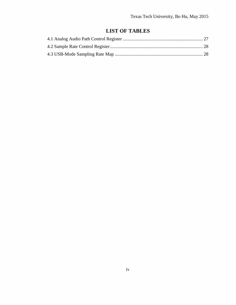
LIST OF TABLES

4.1 Analog Audio Path Control Register ..................................................................... 27

4.2 Sample Rate Control Register ................................................................................ 28

4.3 USB-Mode Sampling Rate Map ............................................................................ 28


v

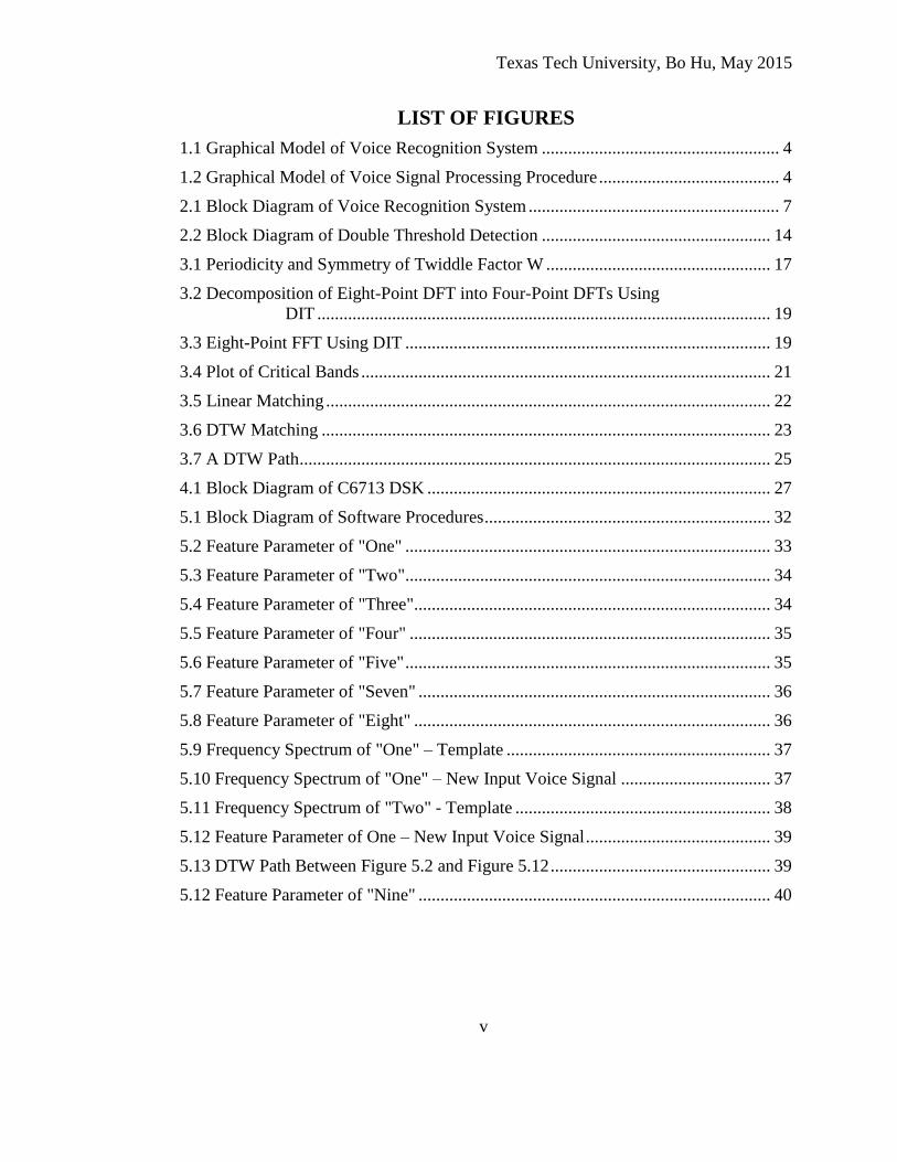
LIST OF FIGURES

1.1 Graphical Model of Voice Recognition System ...................................................... 4

1.2 Graphical Model of Voice Signal Processing Procedure ......................................... 4

2.1 Block Diagram of Voice Recognition System ......................................................... 7

2.2 Block Diagram of Double Threshold Detection .................................................... 14

3.1 Periodicity and Symmetry of Twiddle Factor W ................................................... 17

3.2 Decomposition of Eight-Point DFT into Four-Point DFTs Using

DIT ....................................................................................................... 19

3.3 Eight-Point FFT Using DIT ................................................................................... 19

3.4 Plot of Critical Bands ............................................................................................. 21

3.5 Linear Matching ..................................................................................................... 22

3.6 DTW Matching ...................................................................................................... 23

3.7 A DTW Path ........................................................................................................... 25

4.1 Block Diagram of C6713 DSK .............................................................................. 27

5.1 Block Diagram of Software Procedures ................................................................. 32

5.2 Feature Parameter of "One" ................................................................................... 33

5.3 Feature Parameter of "Two" ................................................................................... 34

5.4 Feature Parameter of "Three" ................................................................................. 34

5.5 Feature Parameter of "Four" .................................................................................. 35

5.6 Feature Parameter of "Five" ................................................................................... 35

5.7 Feature Parameter of "Seven" ................................................................................ 36

5.8 Feature Parameter of "Eight" ................................................................................. 36

5.9 Frequency Spectrum of "One" – Template ............................................................ 37

5.10 Frequency Spectrum of "One" – New Input Voice Signal .................................. 37

5.11 Frequency Spectrum of "Two" - Template .......................................................... 38

5.12 Feature Parameter of One – New Input Voice Signal .......................................... 39

5.13 DTW Path Between Figure 5.2 and Figure 5.12 .................................................. 39

5.12 Feature Parameter of "Nine" ................................................................................ 40


1

CHAPTER I

INTRODUCTION

Background

Voice plays a very important role in human intelligence. It is the most

convenient and basic method for people to communicate with each other. Thus, people

would appreciate voice as a method to communicate with computers. With the rapid

development of computer science and digital signal processing, voice recognition

technology has entered a mature period. The basic research object of voice recognition

is voice signal. The purpose of a voice recognition system is to tell the differences

between different voice signals. Voice recognition is a very important research field in

voice signal processing. Voice recognition is the ability of machines to recognize a

spoken command. Voice recognition systems can be classified into two categories:

speaker-dependent and speaker-independent. Speaker-dependent systems work by

comparing an input word with a user-supplied pattern. The user-supplied pattern is

computed during a pattern training exercise. Speaker-independent systems do not

require a pattern training exercise. Voice recognition systems can be classified by

recognition method into three categories: feature block matching, stochastic modeling

and probability analysis. Moreover, we can choose different objects to recognize, such

as isolated words, phonemes, syllables, isolated sentences and continuous voice.

A voice signal is processed through digital signal processing. In our highly

developed information society, using a digital method to do voice signal transmission,

voice signal storage, voice signal recognition, voice signal synthesis, and voice signal

enhancement is the most important and basic part of our digital communication

networks. Digital processing has some advantages over analog processing: (1) digital

processing techniques can perform very complicated signal analysis, (2) a voice signal

is a combination of phonemes, so it is can be viewed as a discrete signal, (3) a digital

system is reliable, fast, inexpensive, and can easily perform a real-time task, (4) digital


2

voice signals can be transmitted in a channel with strong interference, and it is easy to

encrypt a digital voice signal. Two representations of a voice digital signal are by

waveform and by parameter. Waveform representation represents the waveform of an

analog voice signal after sampling and quantization. Parameter representation

represents the voice signal as the output of a voice model after analysis and

processing.

Voice recognition offers many advantages, including:

(1) Use of voice recognition systems to deliver message is faster and more

direct than communication with script and image.

(2) Using voice recognition systems can completely free eyes and hands.

When driving or doing activities in which both eyes and hands are

required, a voice recognition system can deliver messages and control other

devices. This is true especially under certain circumstance where one can

only hear and speak.

(3) Voice recognition systems are easy to embed in an operating system and

control system.

Research history and recent advances

In the 1960’s, the use of the computer motivated the development of voice

recognition. Swedish scientist Fant’s paper about the acoustic theory of speech

production[13] laid the foundation establishing the digital model of a voice signal.

Some very important digital signal processing theories and algorithms such as digital

signal filters and fast Fourier transforms were developed during the same period.

Those theories and algorithms are the theoretical and technical foundation of voice

digital signal processing.

In the 1970’s, some research achievements had a significant impact on the

improvement and development of voice signal processing. Itakura put forward a

dynamic time warping technique[12] to achieve timing matching between input voice


3

signal and reference template. This technique created a new idea in research of

matching algorithms. A voice compression and feature extraction technique, linear

predictive coding, was used in voice signal processing. It became the most efficient

tool and was widely used in voice signal analysis and voice signal synthesis. In the

same frame time, the hidden Markov model was developed for other applications.

In the 1980’s, a new high-efficiency data compression technique based on

cluster analysis called vector quantization was used in voice recognition, voice coding

and speaker recognition. Another breakthrough was application of the hidden Markov

model to describe voice signals. The hidden Markov model turned voice recognition

algorithms from pattern matching into statistical models. It allowed engineers to build

superior voice recognition systems statistically.

In the 1990’s, research into artificial neural networks, the improvements of

vector quantization techniques, and hidden Markov models and inexpensive

microprocessors again promoted the application and development of digital voice

processing techniques.

Voice signal processing is interdisciplinary. It is a combination of digital signal

processing and phonetics. Developments in either field pushed voice signal processing

forward. Voice signal processing requires a high-speed digital signal processor to

perform the complicated algorithms and do real-time processing. That is one of the

main reasons that digital signal processors were designed and improved. They all help

each other to move forward.

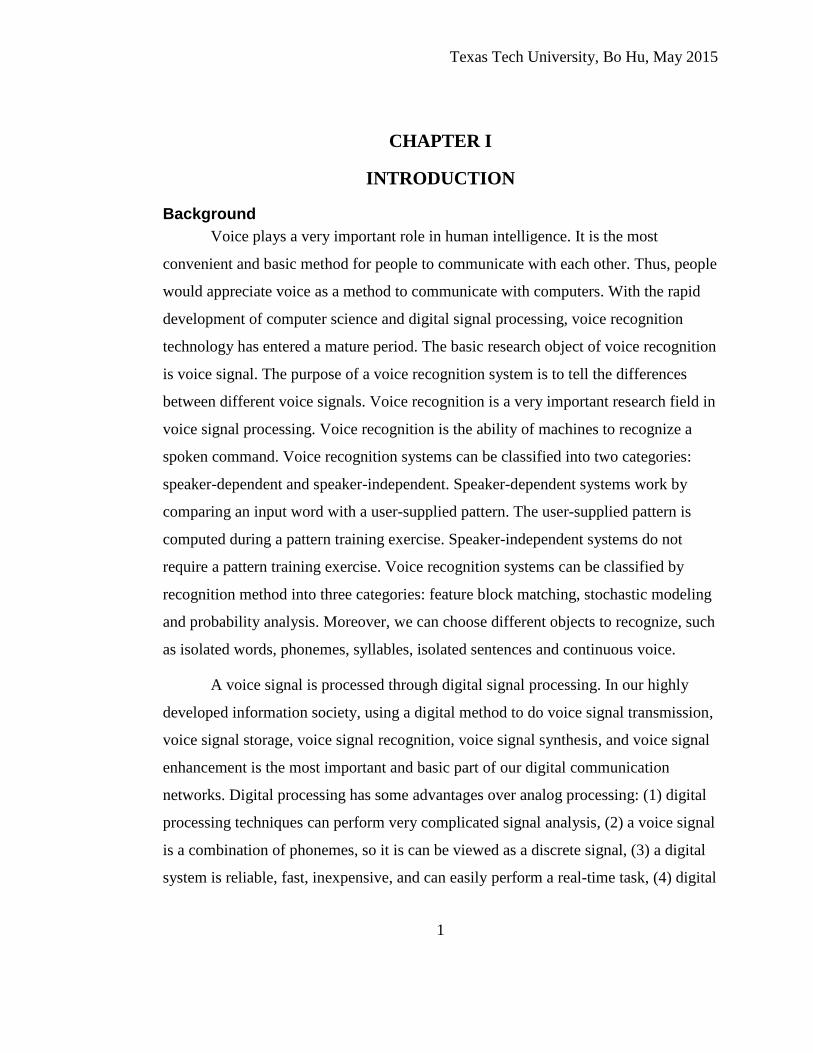
System structure and function

This system will use LEDs to show the input voice signals. First, the stereo

audio codec samples the input voice signal from a microphone. Second, the codec

passes the digital signal to the digital signal processor and the digital signal processor

analyzes the signal. Finally, the digital signal processor controls the LEDs to show the

input voice signal. At the same time, the four DIP switches control the whole system


4

to reset templates, collect the input voice signal, and process the input voice signal.

Figure 1.1 shows the relationship of every component in this system.

Fig 1.1 Graphical Model of Voice Recognition System

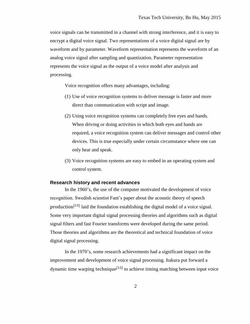
The key component of the system is the digital signal processor, the

TMS320C6713. The C6713 performs all the digital signal processing in this system.

The process can be divided into three modules: preprocessing, feature vector

extraction, and pattern matching. Figure 1.2 below shows the voice signal processing

procedures of this system.

Fig 1.2 Graphical Model of Voice Signal Processing Procedure

In this thesis, the software design of this voice recognition system will be

mainly discussed. TMS320C6713 DSK is the hardware used in this design. The

C6713 digital signal processer, AIC CODEC, LEDs, and DIP switches are embedded

on the C6713 DSK. The following chapters will discuss:

Input

voice

signal

Preprocessing Feature vector

extraction Pattern matching

Microphone AIC CODEC

Digital

Signal

Processor

LEDs

DIP

Switches


5

(1) Analysis of the structure and components of a voice recognition

system.

(2) A method to achieve start and end point detection. A method that

analyzes short-time power and short-time zero-crossing rate is used to

minimize the interference of noise in this system.

(3) Feature parameter extraction using critical bands.

(4) Analysis of a method to achieve pattern matching. A dynamic time

warping algorithm is used to correct the non-linear differences between

two voice signals.

(5) Software design of the voice recognition system.


6

CHAPTER II

BASIC THEORY OF VOICE RECOGNITION

Basic knowledge of voice signal

Voice is a special kind of sound wave, generated by humans and composed of

a series of phonemes. It has some physical features, such as:

(1) Tone, which depends on the frequency of the sound wave.

(2) Loudness, also called volume, which depends on the amplitude of the

sound wave.

(3) Duration, the epoch over which the sound wave is generated.

Three methods are used to generate three different sound types. They are called

voiced sound, unvoiced sound, and plosive. Based on the different mechanisms of

generating a sound, the voice signal can be simulated by a linear time-varying system.

Structure of an isolated word recognition system

The basic processing unit of an isolated word recognition system is a single

discontinuous word. An isolated word recognition system is composed of three

modules. They are the preprocessing module, the feature vector extraction module and

the pattern matching module.

Pre-emphasis, windowing and start-point and end-point detection are

completed in the preprocessing module. They all have significant influence on the

system performance. Windowing segments the input voice signal into continuous

pieces, so that the input voice signal can be analyzed piece by piece. Start-point and

end-point detection determines the start and end of useful input voice signal and

ignores insignificant signals. It reduces computation and increases accuracy of the

system. If preprocessing doesn’t work well or the right start and end can’t be found,

we can’t calculate an accurate feature vector. Moreover, we will likely get poor results

after pattern matching.


7

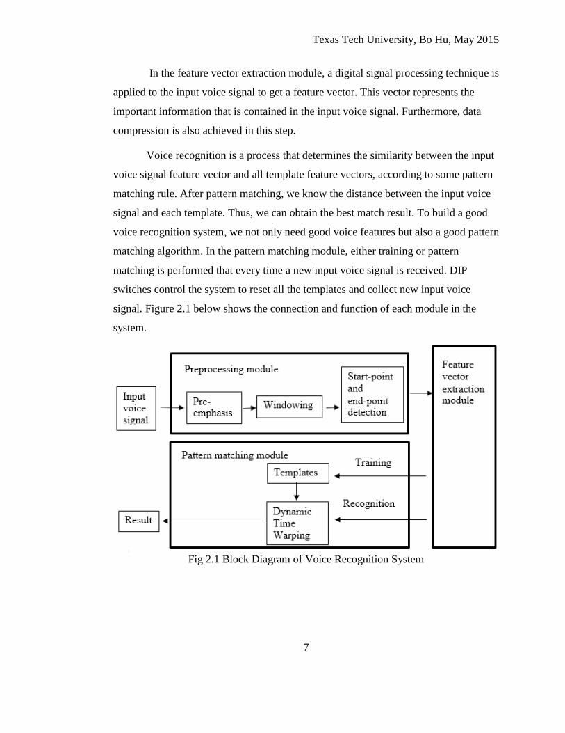
In the feature vector extraction module, a digital signal processing technique is

applied to the input voice signal to get a feature vector. This vector represents the

important information that is contained in the input voice signal. Furthermore, data

compression is also achieved in this step.

Voice recognition is a process that determines the similarity between the input

voice signal feature vector and all template feature vectors, according to some pattern

matching rule. After pattern matching, we know the distance between the input voice

signal and each template. Thus, we can obtain the best match result. To build a good

voice recognition system, we not only need good voice features but also a good pattern

matching algorithm. In the pattern matching module, either training or pattern

matching is performed that every time a new input voice signal is received. DIP

switches control the system to reset all the templates and collect new input voice

signal. Figure 2.1 below shows the connection and function of each module in the

system.

Fig 2.1 Block Diagram of Voice Recognition System

Recognition


8

Time domain analysis of voice signal

Voice is a time domain signal. To analyze a voice signal, the waveform in the

time domain is the most direct approach. Time domain analysis is usually used to do

basic parameter analysis, voice signal segmentation, preprocessing and classification.

The characteristics of time domain analysis are:

(1) It is very straightforward, and it has very clear physical significance.

(2) It is relatively easy to achieve, and it requires less computation.

(3) It can obtain some very important parameters of the voice signal.

Sampling of a voice signal

According to the Nyquist sampling theorem, if an analog signal has a limited

frequency spectrum bandwidth and has the maximum frequency component at

frequency 𝐹𝑚𝑎𝑥, the original analog signal can be exactly recovered from the sampled

signal if the analog signal is sampled at a frequency that is not less than 2𝐹𝑚𝑎𝑥. In

terms of voice signal, the frequency spectrum of voiced sound goes down rapidly at

frequencies higher than 4 kHz, but the frequency spectrum of unvoiced sound doesn’t

go down at frequencies higher than 4 kHz. On the contrary, the frequency spectrum of

unvoiced sound continues to go up, and it doesn’t go down until 8 kHz. Therefore, to

represent a voice signal accurately, signals under 10 kHz should be preserved, and a

sampling frequency of at least 20 kHz is needed. According to some experiments,

however, 5.7 kHz is approximately the maximum frequency that has a significant

influence on clarity and analyzability of a voice signal. The international

telecommunication union proposes to only use the voice signal component under the

frequency of 3.4 kHz, requiring a sampling frequency of 8 kHz in a voice code-decode

system. Theoretically, this damages the clarity of the voice signal. However, it only

loses information about a few unvoiced sounds, and voice signal has a very high

redundancy. The voice signal can still be understood even information from a few

unvoiced sounds is lost.


9

Pre-emphasis

Glottal excitation has an influence on the average power spectrum of a voice

signal. When the voice signal comes out, there is a 6dB/octave attenuation. Therefore,

the high frequency components of the voice signal should be enhanced before the

voice signal is analyzed. This step helps to reduce the influence of noise, improve the

signal to noise ratio, and obtain a better frequency spectrum. Usually, it can be

achieved by using a digital filter to pre-emphasize the input voice signal. The filter is a

first order filter shown below:

H(Z) = 1 – a𝑍−1

y(n) = x(n) – a * x(n-1)

x(n) is the original input voice sequence, y(n) is the pre-emphasis sequence, and a is

the pre-emphasis coefficient. Usually the value of coefficient a is between 0.9-1.0. In

this application, coefficient a is 0.95.

Windowing

Voice signal is a typical non-stationary signal that varies with time. When we

analyze a voice signal, we tend to do so on only a small portion of it. The reason for

this is that we typically assume that the voice signal is a short-time stationary signal

during the time span of our analysis. Hence, the physical feature parameters of the

voice signal are approximately constant during that time span. Thus, we can apply

several kinds of short-time analysis methods to voice signals. Because, voice signal

varies rapidly, we have to cut it into small frames to analyze. Analyzing each frame of

the voice signal allows analysis of a continuous voice signal. Hence, we window the

input voice signal before analysis. There is a little overlap between each continuous

frame, and the process result from a frame of signal is usually a number or an array.

Windowing can be seen as multiplying a voice signal by a series of coefficients that

are zeros except for the region of interest. We can ignore all of the zeros and focus on

the windowed part of the input signal.


10

y(n) = x(n) * w(n)

The expression above shows how windowing is done to an input signal. x(n) is

the input voice signal sequence, w(n) is the window sequence, and y(n) is the output

sequence after windowing. If the coefficients of the window are not constant, there

will be some kind of weighting applied to the signal. The most frequently used

window functions are rectangular window, Hanning window and Hamming window.

The function of each window is showed below:

(1) Rectangular window 𝑤(𝑛) = {1; 0 ≤ 𝑛 ≤ 𝐿 − 1

0; 𝑜𝑡ℎ𝑒𝑟𝑤𝑖𝑠𝑒

(2) Hanning window 𝑤(𝑛) = {0.5 [1 − cos (

2𝜋𝑛

𝐿−1)] ; 0 ≤ 𝑛 ≤ 𝐿 − 1


(3) Hamming window 𝑤(𝑛) = {0.54 − 0.46 cos (

2𝜋𝑛

𝐿−1) ; 0 ≤ 𝑛 ≤ 𝐿 − 1


L is the length of the window. Multiplying the input voice signal by the

window in the time domain is equivalent to the convolution between Fourier

transforms of the input voice signal and the window in the frequency domain.

Generally, we want the window to have high frequency identification rate, which

requires a narrow main lobe, and want less spectrum leakage, which requires

significant attenuation in the side lobes. A rectangular window has a very narrow main

lobe, but the abrupt change at the edge can cause distortion in the signal. To reduce the

distortion, we can use a smoother window. The Hanning window is a raised cosine

window. It has small side lobes but a wide main lobe. The Hamming window is an

improved cosine window. The attenuation of the first side lobe of a Hamming window

is 42 dB, and it has a relatively high frequency identification rate. Therefore, the

Hamming window is chosen for this voice recognition system.

Start and end point detection

The purpose of start and end point detection is to determine the existence of

input voice signal. If it exists, the start and end point are detected and determined. We


11

only need to analyze the signal between the start and end point. An effective start and

end point detection can reduce the processing time of the system and reduce noise

interference. It ensures the performance of the whole system.

Generally, there are two ways to detect the start point and the end point, short-

time power and short-time zero-crossing rate. In this voice recognition system, a

combination of these two methods is used to reduce noise interference.

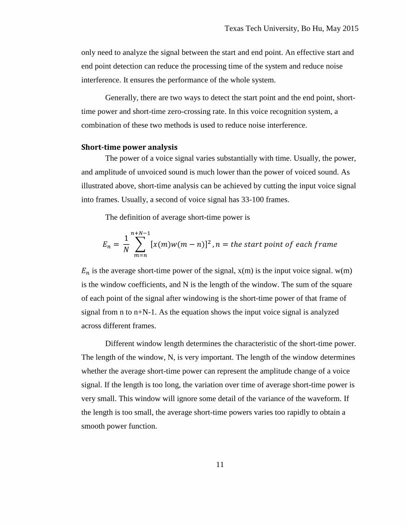
Short-time power analysis

The power of a voice signal varies substantially with time. Usually, the power,

and amplitude of unvoiced sound is much lower than the power of voiced sound. As

illustrated above, short-time analysis can be achieved by cutting the input voice signal

into frames. Usually, a second of voice signal has 33-100 frames.

The definition of average short-time power is

𝐸𝑛 = 1

𝑁∑ [𝑥(𝑚)𝑤(𝑚 − 𝑛)]2

𝑛+𝑁−1

𝑚=𝑛

, 𝑛 = 𝑡ℎ𝑒 𝑠𝑡𝑎𝑟𝑡 𝑝𝑜𝑖𝑛𝑡 𝑜𝑓 𝑒𝑎𝑐ℎ 𝑓𝑟𝑎𝑚𝑒

𝐸𝑛 is the average short-time power of the signal, x(m) is the input voice signal. w(m)

is the window coefficients, and N is the length of the window. The sum of the square

of each point of the signal after windowing is the short-time power of that frame of

signal from n to n+N-1. As the equation shows the input voice signal is analyzed

across different frames.

Different window length determines the characteristic of the short-time power.

The length of the window, N, is very important. The length of the window determines

whether the average short-time power can represent the amplitude change of a voice

signal. If the length is too long, the variation over time of average short-time power is

very small. This window will ignore some detail of the variance of the waveform. If

the length is too small, the average short-time powers varies too rapidly to obtain a

smooth power function.


12

Short-time zero-crossing rate analysis

The zero-crossing rate is the number of occurrence per unit time that the input

voice signal changes sign. The mathematical definition of short-time zero-crossing

rate is:

𝑍𝑛 = 1

2∑ |𝑠𝑔𝑛[𝑥(𝑚)] − 𝑠𝑔𝑛[𝑥(𝑚 − 1)]|

𝑛+𝑁−1

𝑚=𝑛

, 𝑛 = 𝑡ℎ𝑒 𝑠𝑡𝑎𝑟𝑡 𝑝𝑜𝑖𝑛𝑡 𝑜𝑓 𝑒𝑎𝑐ℎ 𝑓𝑟𝑎𝑚𝑒

sgn[] is a sign function:

𝑠𝑔𝑛[𝑥(𝑛)] {1, 𝑥(𝑛) ≥ 0

−1, 𝑥(𝑛) < 0,

x(n) is the input voice signal, 𝑍𝑛 is the zero-crossing rate, factor N is the length of a

frame. As the equation above shows, if there is a sign change, 𝑍𝑛 will increment by 1,

and if there isn’t a sign change, 𝑍𝑛 will increment by 0. Every time after calculating

the value of this expression, |𝑠𝑔𝑛[𝑥(𝑚)] − 𝑠𝑔𝑛[𝑥(𝑚 − 1)]|, the value of m will

increment by 1. We can go through every point of one frame when factor m varies

from n to n+N-1. The value of 𝑍𝑛 is the short-time zero-crossing rate after every point

in the frame is used in the calculation.

Double threshold detection

Double threshold detection uses average short-time power and short-time zero-

crossing rate together to determine the start and end point. Under a high signal to noise

ratio, the start and end point can be easily determined by using average short-time

power alone. But in fact, we don’t usually have a very good signal to noise ratio. It is

inaccurate to use average short-time power alone to determine the start and end point

when the voice signal and background noise is similar. Because the power of the noise

varies substantially over time just like the input voice signal. Double threshold

detection considers that a real input voice signal produces a relatively big average

short-time power.


13

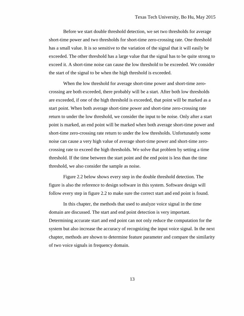
Before we start double threshold detection, we set two thresholds for average

short-time power and two thresholds for short-time zero-crossing rate. One threshold

has a small value. It is so sensitive to the variation of the signal that it will easily be

exceeded. The other threshold has a large value that the signal has to be quite strong to

exceed it. A short-time noise can cause the low threshold to be exceeded. We consider

the start of the signal to be when the high threshold is exceeded.

When the low threshold for average short-time power and short-time zero-

crossing are both exceeded, there probably will be a start. After both low thresholds

are exceeded, if one of the high threshold is exceeded, that point will be marked as a

start point. When both average short-time power and short-time zero-crossing rate

return to under the low threshold, we consider the input to be noise. Only after a start

point is marked, an end point will be marked when both average short-time power and

short-time zero-crossing rate return to under the low thresholds. Unfortunately some

noise can cause a very high value of average short-time power and short-time zero-

crossing rate to exceed the high thresholds. We solve that problem by setting a time

threshold. If the time between the start point and the end point is less than the time

threshold, we also consider the sample as noise.

Figure 2.2 below shows every step in the double threshold detection. The

figure is also the reference to design software in this system. Software design will

follow every step in figure 2.2 to make sure the correct start and end point is found.

In this chapter, the methods that used to analyze voice signal in the time

domain are discussed. The start and end point detection is very important.

Determining accurate start and end point can not only reduce the computation for the

system but also increase the accuracy of recognizing the input voice signal. In the next

chapter, methods are shown to determine feature parameter and compare the similarity

of two voice signals in frequency domain.


14

Start

Calculate average short-time power and short-time zero-crossing rate

Larger than both

low thresholds

Yes

No

Next frame of signal

Mark start point

Larger than one of the high

threshold in next 3 frames Cancel start point

No

Yes

Calculate average short-time power and short-time zero-crossing rate

Smaller than both

low thresholds

No

Next frame of signal

Yes

Mark end point

End

Fig 2.2 Block Diagram of Double Threshold Detection


15

CHAPTER III

FREQUENCY DOMAIN ANALYSIS

Short-time Fourier analysis

In voice signal analysis, the Fourier transform is a very helpful tool to analyze

the frequency components. Some features of the voice signal can be obtained from the

frequency spectrum. The short-time Fourier transform is applied to short-time Fourier

analysis.

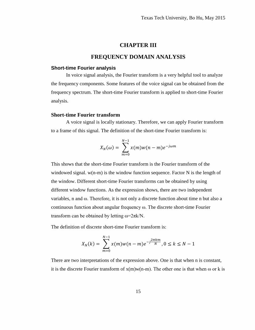
Short-time Fourier transform

A voice signal is locally stationary. Therefore, we can apply Fourier transform

to a frame of this signal. The definition of the short-time Fourier transform is:

𝑋𝑁(𝜔) = ∑ 𝑥(𝑚)𝑤(𝑛 − 𝑚)𝑒−𝑗𝜔𝑚

𝑁−1

𝑚=0

This shows that the short-time Fourier transform is the Fourier transform of the

windowed signal. w(n-m) is the window function sequence. Factor N is the length of

the window. Different short-time Fourier transforms can be obtained by using

different window functions. As the expression shows, there are two independent

variables, n and ω. Therefore, it is not only a discrete function about time n but also a

continuous function about angular frequency ω. The discrete short-time Fourier

transform can be obtained by letting ω=2πk/N.

The definition of discrete short-time Fourier transform is:

𝑋𝑁(𝑘) = ∑ 𝑥(𝑚)𝑤(𝑛 − 𝑚)𝑒−𝑗2𝜋𝑘𝑚

𝑁

𝑁−1

𝑚=0

, 0 ≤ 𝑘 ≤ 𝑁 − 1

There are two interpretations of the expression above. One is that when n is constant,

it is the discrete Fourier transform of x(m)w(n-m). The other one is that when ω or k is


16

constant, 𝑋𝑁(𝑘) can be seen as a function of time n. It is the convolution of the voice

signal and the window.

Fast Fourier transform

The fast Fourier transform is a highly efficient algorithm used to convert a time

domain signal into a frequency domain signal. The fast Fourier transform requires less

computation than discrete Fourier transform, and is easier to implement on a digital

signal processor.

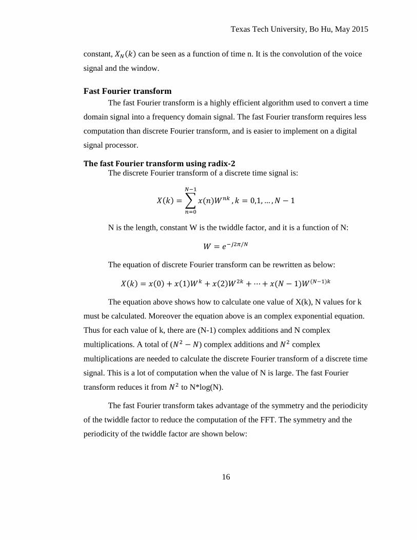
The fast Fourier transform using radix-2 The discrete Fourier transform of a discrete time signal is:

𝑋(𝑘) = ∑ 𝑥(𝑛)𝑊𝑛𝑘

𝑁−1

𝑛=0

, 𝑘 = 0,1, … , 𝑁 − 1

N is the length, constant W is the twiddle factor, and it is a function of N:

𝑊 = 𝑒−𝑗2𝜋/𝑁

The equation of discrete Fourier transform can be rewritten as below:

𝑋(𝑘) = 𝑥(0) + 𝑥(1)𝑊𝑘 + 𝑥(2)𝑊2𝑘 + ⋯ + 𝑥(𝑁 − 1)𝑊(𝑁−1)𝑘

The equation above shows how to calculate one value of X(k), N values for k

must be calculated. Moreover the equation above is an complex exponential equation.

Thus for each value of k, there are (N-1) complex additions and N complex

multiplications. A total of (𝑁2 − 𝑁) complex additions and 𝑁2 complex

multiplications are needed to calculate the discrete Fourier transform of a discrete time

signal. This is a lot of computation when the value of N is large. The fast Fourier

transform reduces it from 𝑁2 to N*log(N).

The fast Fourier transform takes advantage of the symmetry and the periodicity

of the twiddle factor to reduce the computation of the FFT. The symmetry and the

periodicity of the twiddle factor are shown below:


17

𝑊𝑘+𝑁 = 𝑊𝑘 (periodicity)

𝑊𝑘+𝑁/2 = −𝑊𝑘 (symmetry)

As the equations above show, periodicity means 𝑊𝑘 will be the same value N

points later, and 𝑊𝑛𝑘 will be the opposite value N/2 points later. Figure 3.1 shows an

example of the periodicity and the symmetry of the twiddle factor W for N=8.

Fig 3.1 Periodicity and Symmetry of Twiddle Factor 𝑊[3]

For different value of k, we can obtain 𝑊9 = 𝑊1, 𝑊10 = 𝑊2, and so on.

For a radix-2, the fast Fourier transform decomposes an N point DFT into two

N/2 point DFTs. And each N/2 point DFT is further decomposed into two N/4 point

DFTs. The decomposition ends when an N point DFT is decomposed into N/2 two

point DFTs. For a radix-2 FFT, N must be the power of 2, and the last decomposition

is two point DFT.

Decimation-in-time (DIT) radix-2 fast Fourier transform Decimation-in-time decomposes the input sequence into smaller subsequences.

DIT decomposes the input sequence into an even sequence and an odd sequence. Thus

we can rewrite the DFT equation as below:


18

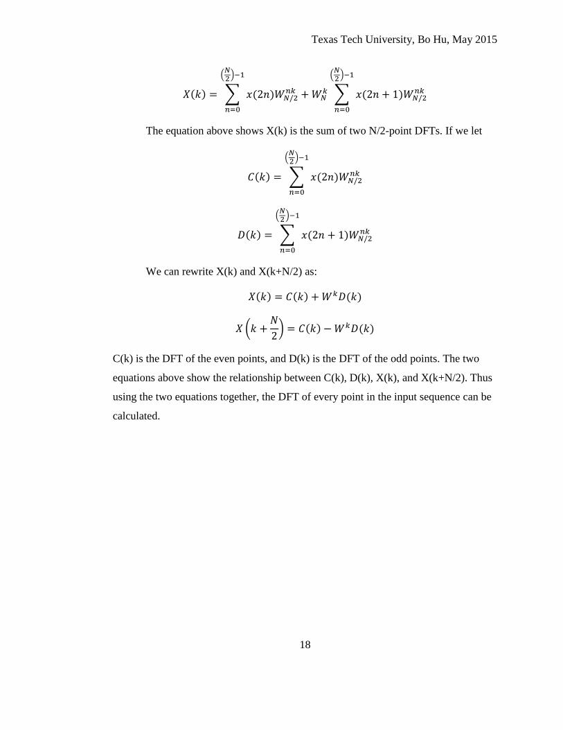
𝑋(𝑘) = ∑ 𝑥(2𝑛)𝑊𝑁/2𝑛𝑘

(𝑁2

)−1

𝑛=0

+ 𝑊𝑁𝑘 ∑ 𝑥(2𝑛 + 1)𝑊𝑁/2

𝑛𝑘

(𝑁2

)−1

𝑛=0

The equation above shows X(k) is the sum of two N/2-point DFTs. If we let

𝐶(𝑘) = ∑ 𝑥(2𝑛)𝑊𝑁/2𝑛𝑘

(𝑁2

)−1

𝑛=0

𝐷(𝑘) = ∑ 𝑥(2𝑛 + 1)𝑊𝑁/2𝑛𝑘

(𝑁2

)−1

𝑛=0

We can rewrite X(k) and X(k+N/2) as:

𝑋(𝑘) = 𝐶(𝑘) + 𝑊𝑘𝐷(𝑘)

𝑋 (𝑘 +𝑁

2) = 𝐶(𝑘) − 𝑊𝑘𝐷(𝑘)

C(k) is the DFT of the even points, and D(k) is the DFT of the odd points. The two

equations above show the relationship between C(k), D(k), X(k), and X(k+N/2). Thus

using the two equations together, the DFT of every point in the input sequence can be

calculated.


19

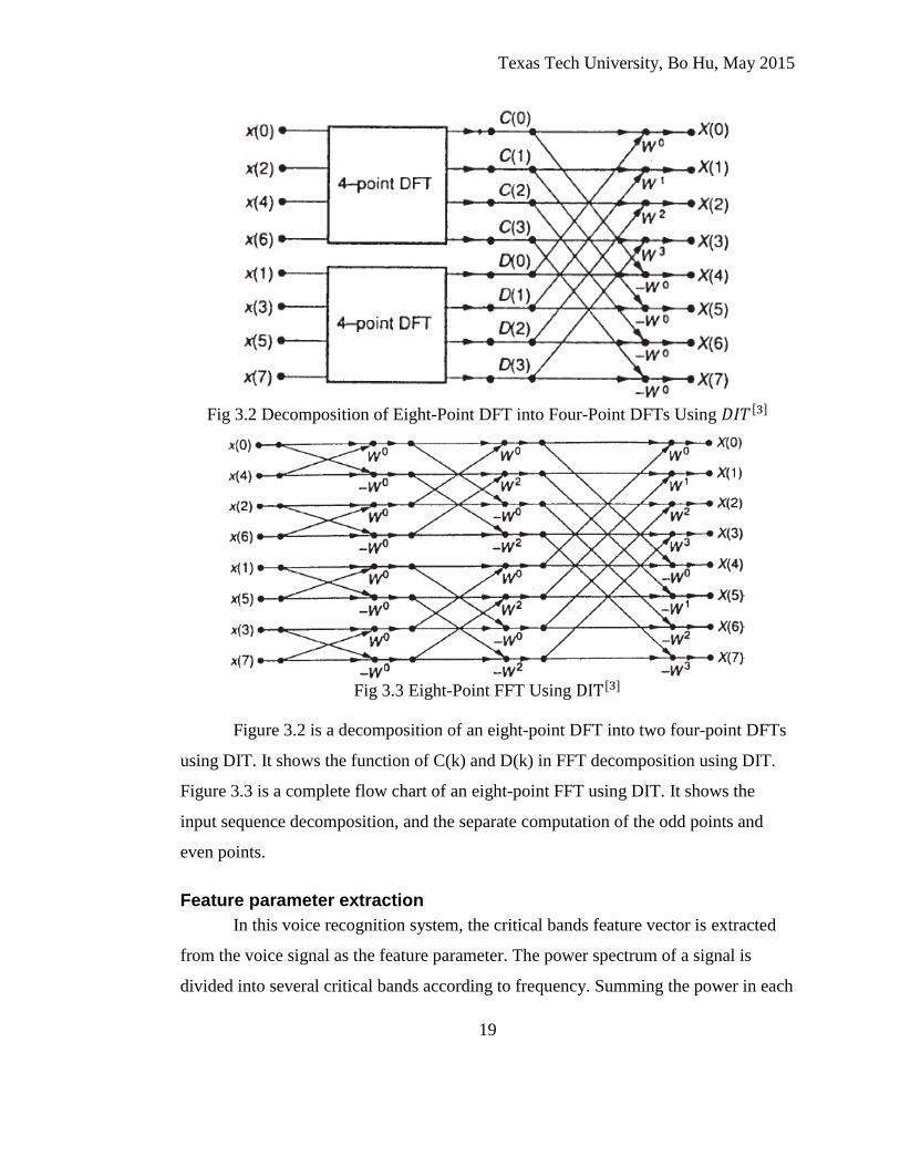
Fig 3.2 Decomposition of Eight-Point DFT into Four-Point DFTs Using 𝐷𝐼𝑇[3]

Fig 3.3 Eight-Point FFT Using DIT[3]

Figure 3.2 is a decomposition of an eight-point DFT into two four-point DFTs

using DIT. It shows the function of C(k) and D(k) in FFT decomposition using DIT.

Figure 3.3 is a complete flow chart of an eight-point FFT using DIT. It shows the

input sequence decomposition, and the separate computation of the odd points and

even points.

Feature parameter extraction

In this voice recognition system, the critical bands feature vector is extracted

from the voice signal as the feature parameter. The power spectrum of a signal is

divided into several critical bands according to frequency. Summing the power in each


20

critical band, we can get a corresponding critical band feature vector. A critical band

feature vector can be calculated for each frame of the input voice signal.

The first step to calculate the critical bands vector is to calculate the power

spectrum. The power spectrum is the square of the absolute value after discrete

Fourier transform of every frame of windowed voice signal. In this case, a 256 point

discrete Fourier transform is performed with a sample frequency of 8 kHz. Thus each

windowed signal is 32 ms.

The second step is to calculate cut-off frequency of each critical band. The cut-

off frequency is calculated by the expression below:

𝑙 = 26.81𝑓�̂�

1960 + 𝑓�̂�

− 0.53

The cut-off frequency can be calculated by setting l from 1 to the value we need. And

the cut-off frequency is larger than zero and less than half of the sample frequency.

Zero and 𝑓1̂ constitute the extents of the first critical band. 𝑓1̂ and 𝑓2̂ constitute the

second critical band. The rest of the critical bands can be done in the same manner.

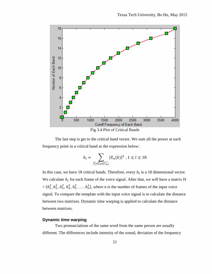
As figure 3.4 below shows, the frequency at each square is the cut-off

frequency for each critical band. The frequency ends at 4 kHz, because 4 kHz is the

maximum frequency we want to analyze in this application. As the figure shows, there

are 18 critical bands in total.


21

Fig 3.4 Plot of Critical Bands

The last step is get to the critical band vector. We sum all the power at each

frequency point in a critical band as the expression below:

ℎ𝑙 = ∑ |𝑋𝑛(𝑘)|2

𝑓�̂�≤𝑓�̂�≤𝑓𝑙+1̂

, 1 ≤ 𝑙 ≤ 18

In this case, we have 18 critical bands. Therefore, every ℎ𝑙 is a 18 dimensional vector.

We calculate ℎ𝑙 for each frame of the voice signal. After that, we will have a matrix H

= [ℎ1𝑇 , ℎ2

𝑇, ℎ3𝑇, ℎ4

𝑇, ℎ5𝑇……ℎ𝑛

𝑇], where n is the number of frames of the input voice

signal. To compare the template with the input voice signal is to calculate the distance

between two matrixes. Dynamic time warping is applied to calculate the distance

between matrixes.

Dynamic time warping

Two pronunciations of the same word from the same person are usually

different. The differences include intensity of the sound, deviation of the frequency


22

spectrum, and the duration of each syllable. Usually the syllables of the two

pronunciations don’t correspond to each other linearly along the time axis. Even

though a person tries to pronounce the word as same as the last time, there will still be

differences. We need to calibrate the feature parameters in time. Dynamic time

warping (DTW) is a pattern matching technique that uses dynamic programming to

solve the non-linear problem between two feature parameters. It works very well in

isolated word recognition.

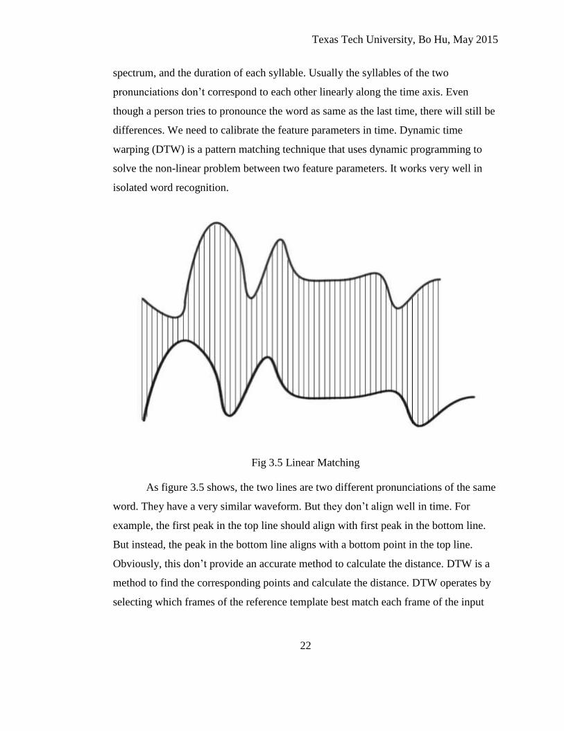
Fig 3.5 Linear Matching

As figure 3.5 shows, the two lines are two different pronunciations of the same

word. They have a very similar waveform. But they don’t align well in time. For

example, the first peak in the top line should align with first peak in the bottom line.

But instead, the peak in the bottom line aligns with a bottom point in the top line.

Obviously, this don’t provide an accurate method to calculate the distance. DTW is a

method to find the corresponding points and calculate the distance. DTW operates by

selecting which frames of the reference template best match each frame of the input


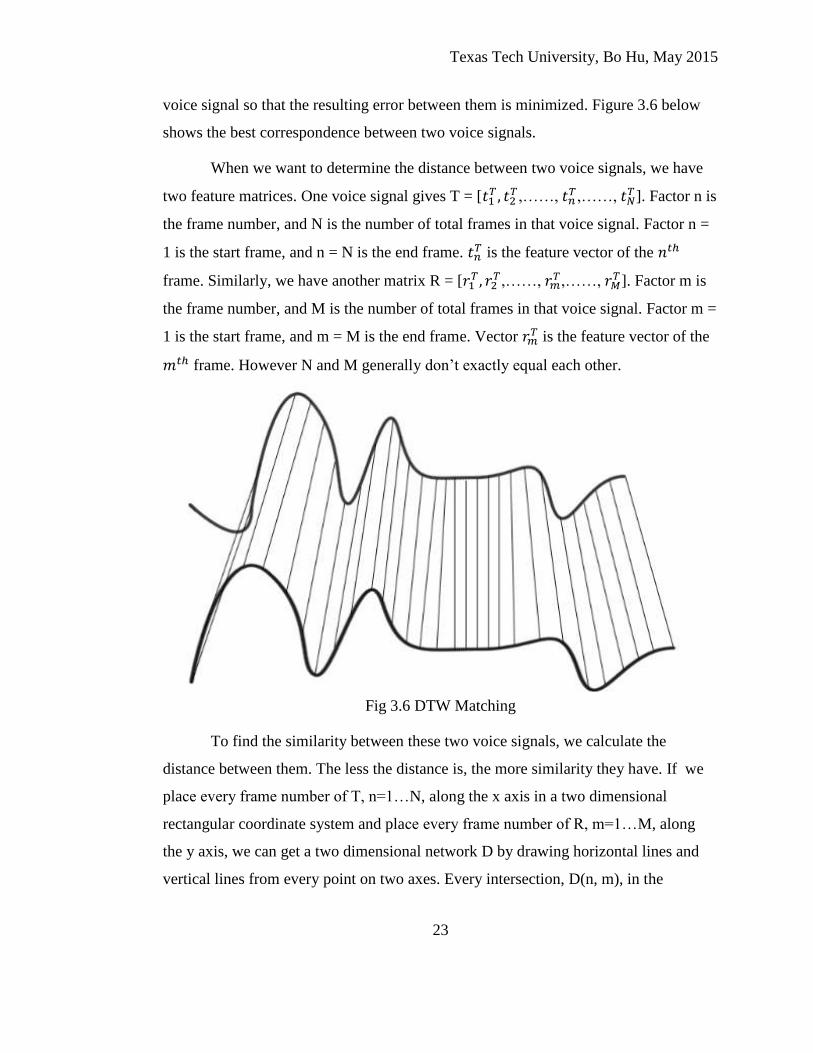
23

voice signal so that the resulting error between them is minimized. Figure 3.6 below

shows the best correspondence between two voice signals.

When we want to determine the distance between two voice signals, we have

two feature matrices. One voice signal gives T = [𝑡1𝑇 , 𝑡2

𝑇,……, 𝑡𝑛𝑇,……, 𝑡𝑁

𝑇]. Factor n is

the frame number, and N is the number of total frames in that voice signal. Factor n =

1 is the start frame, and n = N is the end frame. 𝑡𝑛𝑇 is the feature vector of the 𝑛𝑡ℎ

frame. Similarly, we have another matrix R = [𝑟1𝑇 , 𝑟2

𝑇,……, 𝑟𝑚𝑇,……, 𝑟𝑀

𝑇]. Factor m is

the frame number, and M is the number of total frames in that voice signal. Factor m =

1 is the start frame, and m = M is the end frame. Vector 𝑟𝑚𝑇 is the feature vector of the

𝑚𝑡ℎ frame. However N and M generally don’t exactly equal each other.

Fig 3.6 DTW Matching

To find the similarity between these two voice signals, we calculate the

distance between them. The less the distance is, the more similarity they have. If we

place every frame number of T, n=1…N, along the x axis in a two dimensional

rectangular coordinate system and place every frame number of R, m=1…M, along

the y axis, we can get a two dimensional network D by drawing horizontal lines and

vertical lines from every point on two axes. Every intersection, D(n, m), in the


24

network is the intersection of the 𝑛𝑡ℎ frame in T and the 𝑚𝑡ℎ frame in R. Value of the

intersection, D(n, m), is the Euclidean distance between the 𝑛𝑡ℎ frame in T and the

𝑚𝑡ℎ frame in R. DTW finds the best path to connect the start and the end in the

network. Each frame pair, 𝑛𝑡ℎ and 𝑚𝑡ℎ, to which every point on the path is

corresponding is the frame pair used to calculate the distance between two voice

signals. The path isn’t chosen randomly. There is a defined method to determine the

path.

(1) Every path starts at point (1,1) and ends at point (N,M), because the time

sequence can’t be changed.

(2) If 𝐷𝑘−1 = (𝑎′, 𝑏′), the next point, 𝐷𝑘 = (𝑎, 𝑏), on the path must satisfy,

(𝑎 − 𝑎′) ≤ 1 and (𝑏 − 𝑏′) ≤ 1. Therefore, a point can only be connected

to the point which is adjacent to it. This makes sure that the best path

includes every frame number of both T and R.

(3) If 𝐷𝑘−1 = (𝑎′, 𝑏′), the next point, 𝐷𝑘 = (𝑎, 𝑏), on the path must satisfy,

(𝑎 − 𝑎′) ≥ 0 and (𝑏 − 𝑏′) ≥ 0. Therefore all the points on the path are

monotonic. This makes sure that the lines that connect two voice signals in

Fig 3.2 don’t cross each other.

According to the rules above, if the current point on the path is 𝐷𝑘 = (𝑎, 𝑏),

only three possibilities exist for the previous point, 𝐷𝑘 = (𝑎 − 1, 𝑏 − 1), 𝐷𝑘 = (𝑎 −

1, 𝑏) and 𝐷𝑘 = (𝑎, 𝑏 − 1). Therefore, we can obtain a distance matrix, DIS(N,M),

by:

𝐷𝐼𝑆(𝑛, 𝑚) = 𝐷(𝑛, 𝑚) + min [𝐷𝐼𝑆(𝑛 − 1, 𝑚), 𝐷𝐼𝑆(𝑛, 𝑚 − 1), 𝐷𝐼𝑆(𝑛 − 1, 𝑚 − 1)]

D(n, m) is the Euclidean distance of the 𝑛𝑡ℎ frame in T and the 𝑚𝑡ℎ frame in

R. DIS(n, m) is the shortest distance from D(1, 1) to D(n, m), which means that the

path from D(1, 1) to D(n, m) is the best path, since DIS(n, m) is always the shortest

distance from previous points. Therefore DIS(N, M) is always the shortest distance

from D(1,1) to D(N, M). The path from D(1,1) to D(N, M) is the best path we are

seeking.


25

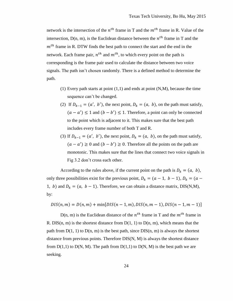
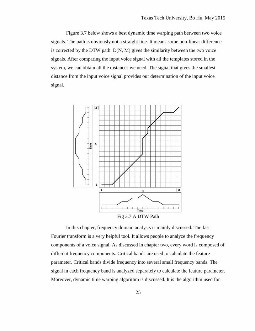
Figure 3.7 below shows a best dynamic time warping path between two voice

signals. The path is obviously not a straight line. It means some non-linear difference

is corrected by the DTW path. D(N, M) gives the similarity between the two voice

signals. After comparing the input voice signal with all the templates stored in the

system, we can obtain all the distances we need. The signal that gives the smallest

distance from the input voice signal provides our determination of the input voice

signal.

Fig 3.7 A DTW Path

In this chapter, frequency domain analysis is mainly discussed. The fast

Fourier transform is a very helpful tool. It allows people to analyze the frequency

components of a voice signal. As discussed in chapter two, every word is composed of

different frequency components. Critical bands are used to calculate the feature

parameter. Critical bands divide frequency into several small frequency bands. The

signal in each frequency band is analyzed separately to calculate the feature parameter.

Moreover, dynamic time warping algorithm is discussed. It is the algorithm used for


26

pattern matching. It corrects the non-linear difference between two voice signals to

obtain the best similarity. So far, the methods that are needed in time domain analysis

and frequency domain analysis have been discussed. In the next chapter, software

design will be discussed.


27

CHAPTER IV

HARDWARE INITIALIZATION

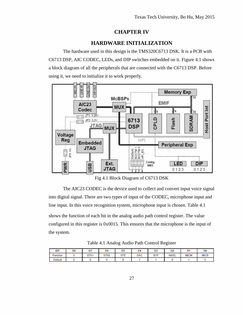
The hardware used in this design is the TMS320C6713 DSK. It is a PCB with

C6713 DSP, AIC CODEC, LEDs, and DIP switches embedded on it. Figure 4.1 shows

a block diagram of all the peripherals that are connected with the C6713 DSP. Before

using it, we need to initialize it to work properly.

Fig 4.1 Block Diagram of C6713 DSK

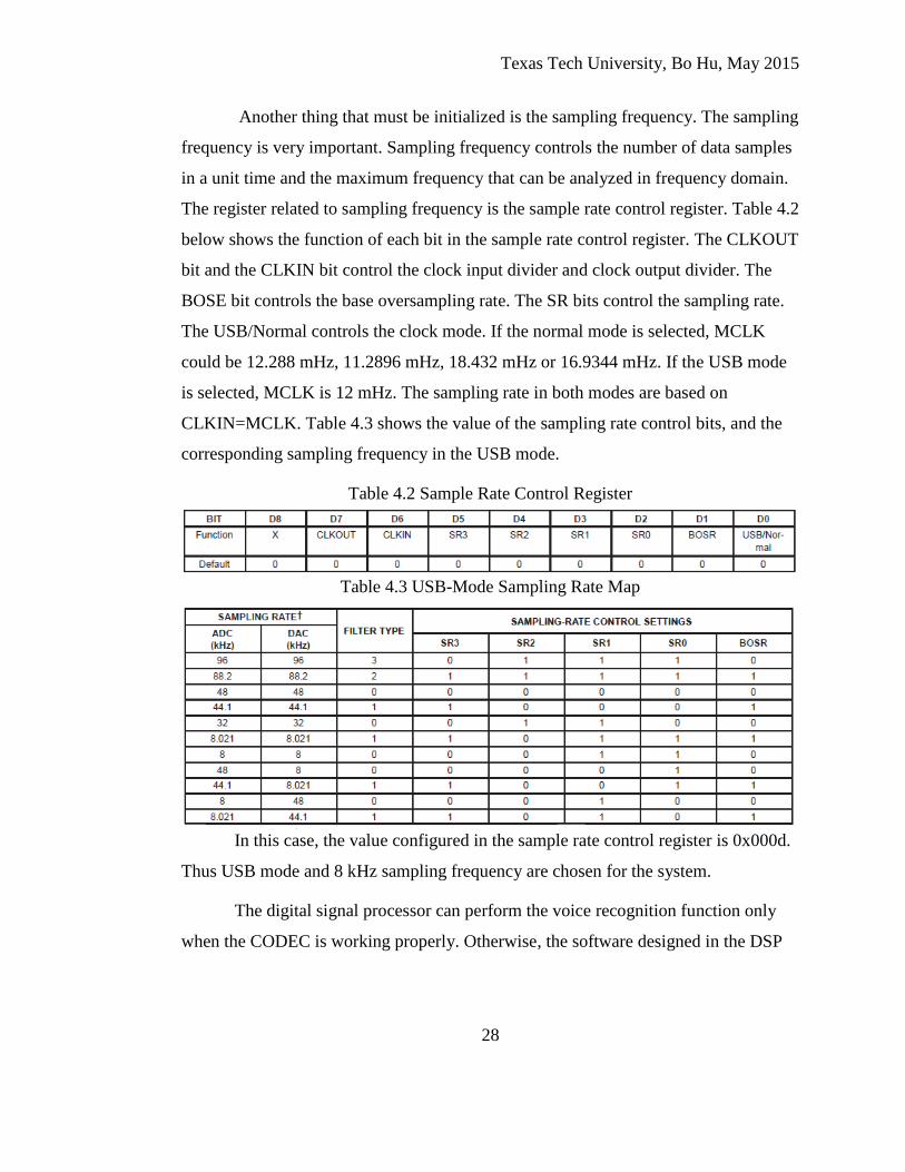
The AIC23 CODEC is the device used to collect and convert input voice signal

into digital signal. There are two types of input of the CODEC, microphone input and

line input. In this voice recognition system, microphone input is chosen. Table 4.1

shows the function of each bit in the analog audio path control register. The value

configured in this register is 0x0015. This ensures that the microphone is the input of

the system.

Table 4.1 Analog Audio Path Control Register


28

Another thing that must be initialized is the sampling frequency. The sampling

frequency is very important. Sampling frequency controls the number of data samples

in a unit time and the maximum frequency that can be analyzed in frequency domain.

The register related to sampling frequency is the sample rate control register. Table 4.2

below shows the function of each bit in the sample rate control register. The CLKOUT

bit and the CLKIN bit control the clock input divider and clock output divider. The

BOSE bit controls the base oversampling rate. The SR bits control the sampling rate.

The USB/Normal controls the clock mode. If the normal mode is selected, MCLK

could be 12.288 mHz, 11.2896 mHz, 18.432 mHz or 16.9344 mHz. If the USB mode

is selected, MCLK is 12 mHz. The sampling rate in both modes are based on

CLKIN=MCLK. Table 4.3 shows the value of the sampling rate control bits, and the

corresponding sampling frequency in the USB mode.

Table 4.2 Sample Rate Control Register

Table 4.3 USB-Mode Sampling Rate Map

In this case, the value configured in the sample rate control register is 0x000d.

Thus USB mode and 8 kHz sampling frequency are chosen for the system.

The digital signal processor can perform the voice recognition function only

when the CODEC is working properly. Otherwise, the software designed in the DSP


29

can’t meet the requirements for the voice recognition system. The final chapter

provides test results and conclusions.


30

CHAPTER V

CONCLUSION

A speaker-dependent isolated word voice recognition system has been

achieved. There are seven templates in this system. The system was tested several

times to recognize seven different words.

Because a microphone is used to collect the input voice signal, noise

interference is inevitable. The sample frequency is 8 kHz and a 12000-point array is

used to store the input voice signal. At most, 1.5 s of input voice signal can be stored,

which is enough for people to speak one word. DIP switches are used to control the

system. DIP 1 is used to reset the stored templates, and DIP 0 is used to control the

system to acquire new input voice signals. LEDs are used to show the recognition

results and the status of the system. When a new input voice signal is acquired, LED0-

LED2 are used to show the recognition results in binary. LED3 is used to show the

status of the system. If it is on, the system is ready for an input signal, and if it is off

the system won’t do anything. If there is an invalid input signal, all the LEDs will be

lighted.

Software procedures

Figure 5.1 shows the software procedures designed in the digital signal

processer for every new input voice signal. If the DIP 0 is down the system will ignore

all the input voice signal from the microphone, and if DIP 0 is up the system will

process the input voice signal. The first procedure is to pre-emphasize the input voice

signal after the system collects enough data. The second procedure is to detect the start

and end point of the significant information in the input voice signal. After we have

the start and end point of the input voice signal, we can calculate the number of frames

during that period of signal. A frame is 256 points long. If the number of frames is

larger than 20, the input voice signal is considered as a valid input signal. If the

number of frames is smaller than 20, the input voice signal is considered as an invalid

input noise. Once we have a valid input voice signal, we convert it into the frequency


31

domain to analyze the frequency components of the signal. After fast Fourier

transform is applied to the signal, the feature parameter is calculated by using the

critical bands. The feature parameter for each frame of input voice signal is an 18

dimensional vector. At this point, if the templates aren’t fully set, the feature

parameter is stored in the corresponding template. If there are enough templates, the

dynamic time warping algorithm is applied to calculate the distance between the input

voice signal and every template. The shortest distance determines the corresponding

template to the input voice signal. However, if the shortest distance is larger than the

distance we can accept, the input voice signal is considered to be invalid noise. The

final procedure is to light the LEDs to show the result. The system will light all LEDs

to show an invalid input voice signal, and light the binary combination of LEDs to

show a valid result. After the system shows the result, the system is ready to process a

new input voice signal.


32

Fig 5.1 Block Diagram of Software Procedures

Start

Collect input

Pre-emphasis and windowing

Enough frames

of input

Yes

No

FFT, and feature parameter extraction

Recognition

Yes

No

Set template

Calculate distance using dynamic time warping

Use LEDs to show result

End

Start and end point detection

Valid

Yes

No

Light all LEDs


33

Result analysis

The system is tested with eight different words: “one”, “two”, “three”, “four”,

“five”, “seven”, “eight”, and “nine”. “One”, “two”, “three’, “four”, “five”, “seven”,

and “eight” are valid input voice signals. The feature parameter of these seven words

are stored in the templates. The word “nine” is a false track used to test whether the

system can identify it as an invalid input voice signal. The word six is not used in the

test, because six has a very unique pronunciation. It ends with two voiceless

consonants, and therefore it is hard to get a valid input signal.

The method used to calculate the feature parameter is discussed above. The

figures below show the feature parameter of each word, “one”, “two”, “three”, “four”,

“five”, “seven”, and “eight”.

Fig 5.2 Feature Parameter of “One”


34

Fig 5.3 Feature Parameter of “Two”

Fig 5.4 Feature Parameter of “Three”


35

Fig 5.5 Feature Parameter of “Four”

Fig 5.6 Feature Parameter of “Five”


36

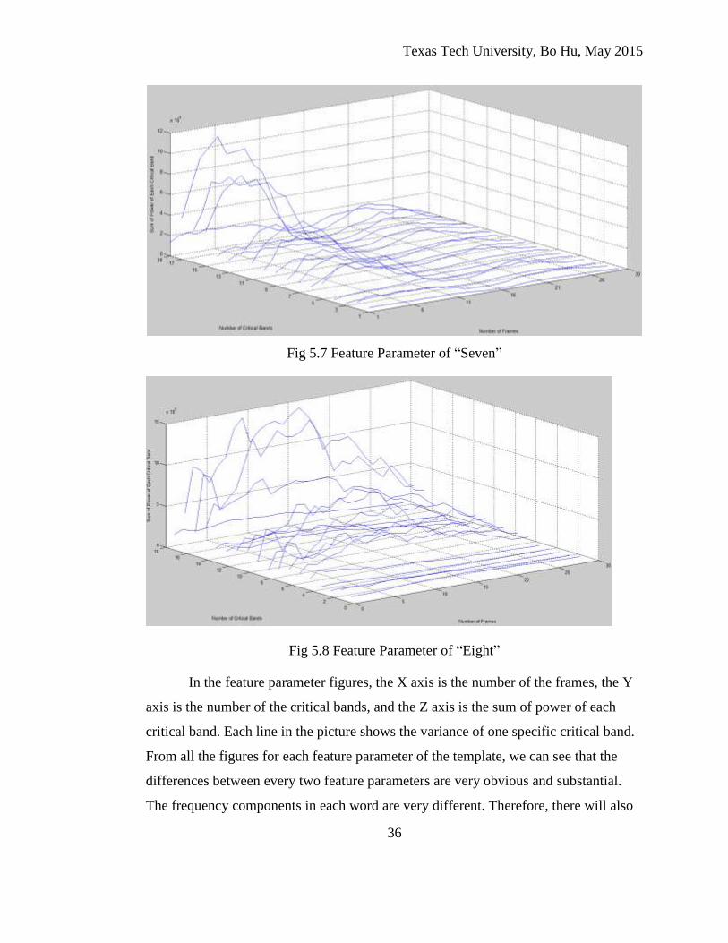
Fig 5.7 Feature Parameter of “Seven”

Fig 5.8 Feature Parameter of “Eight”

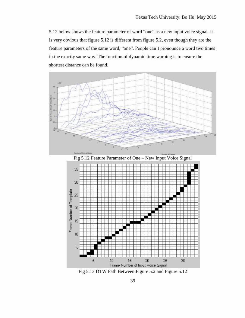
In the feature parameter figures, the X axis is the number of the frames, the Y

axis is the number of the critical bands, and the Z axis is the sum of power of each

critical band. Each line in the picture shows the variance of one specific critical band.

From all the figures for each feature parameter of the template, we can see that the

differences between every two feature parameters are very obvious and substantial.

The frequency components in each word are very different. Therefore, there will also


37

be significant differences in the distances between the input voice signal and every

template. With the differences in the distances, we can tell the similarity between the

input voice signal and every template. The word that has the shortest distance with

input voice signal is the result of the voice recognition. The corresponding LEDs will

be lighted up to show the result.

Fig 5.9 Frequency Spectrum of “One” – Template

Fig 5.10 Frequency Spectrum of “One” – New Input Voice Signal


38

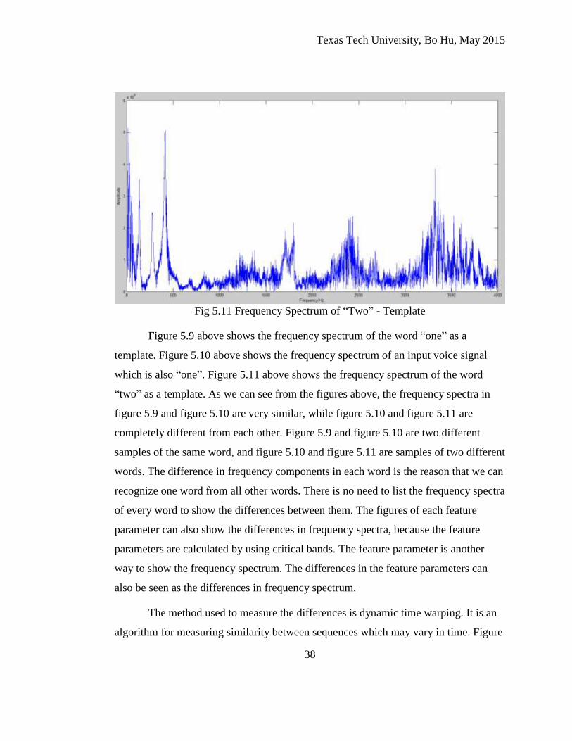
Fig 5.11 Frequency Spectrum of “Two” - Template

Figure 5.9 above shows the frequency spectrum of the word “one” as a

template. Figure 5.10 above shows the frequency spectrum of an input voice signal

which is also “one”. Figure 5.11 above shows the frequency spectrum of the word

“two” as a template. As we can see from the figures above, the frequency spectra in

figure 5.9 and figure 5.10 are very similar, while figure 5.10 and figure 5.11 are

completely different from each other. Figure 5.9 and figure 5.10 are two different

samples of the same word, and figure 5.10 and figure 5.11 are samples of two different

words. The difference in frequency components in each word is the reason that we can

recognize one word from all other words. There is no need to list the frequency spectra

of every word to show the differences between them. The figures of each feature

parameter can also show the differences in frequency spectra, because the feature

parameters are calculated by using critical bands. The feature parameter is another

way to show the frequency spectrum. The differences in the feature parameters can

also be seen as the differences in frequency spectrum.

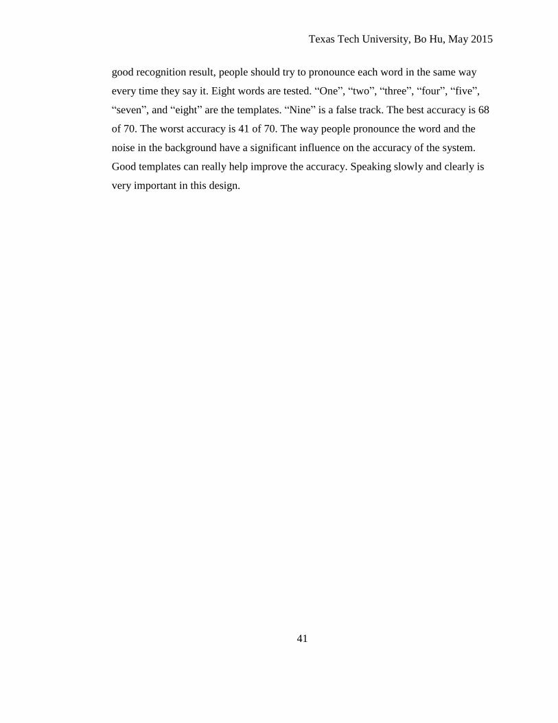
The method used to measure the differences is dynamic time warping. It is an

algorithm for measuring similarity between sequences which may vary in time. Figure


39

5.12 below shows the feature parameter of word “one” as a new input voice signal. It

is very obvious that figure 5.12 is different from figure 5.2, even though they are the

feature parameters of the same word, “one”. People can’t pronounce a word two times

in the exactly same way. The function of dynamic time warping is to ensure the

shortest distance can be found.

Fig 5.12 Feature Parameter of One – New Input Voice Signal

Fig 5.13 DTW Path Between Figure 5.2 and Figure 5.12


40

Figure 5.13 above shows an actual dynamic time warping path between figure

5.2 and figure 5.12. The last grid at the top right corner is always the shortest distance

between two sequences. Even though differences exist between in figure 5.2 and

figure 5.12, the distance between them is still the shortest among all the templates,

from figure 5.2 to figure 5.8. The new input voice signal is recognized correctly.

The word nine is used as a false track in the test. Figure 5.14 below shows the

feature parameter of word nine.

Fig 5.14 Feature Parameter of “Nine”

The feature parameter figures of each word are very intuitive. The feature

parameter of nine is not similar to any other feature parameter of all the templates,

“one”, “two”, “three”, “four”, “five”, “seven”, and “eight”. Thus the shortest distance

between “nine” and all the templates is a very large number. In this case, the input

voice signal is defined as not similar to any template.

If we look carefully, we can find that the feature parameter of “one” is very

similar to the feature parameter of “five”. Usually when the input voice signal is “one”

or “five”, the distance between input signal and feature parameter of “one” is very

close to the distance between input signal and feature parameter of “five”. There is a

possibility that the system may be confused about “one” and “five”. Therefore to get a


41

good recognition result, people should try to pronounce each word in the same way

every time they say it. Eight words are tested. “One”, “two”, “three”, “four”, “five”,

“seven”, and “eight” are the templates. “Nine” is a false track. The best accuracy is 68

of 70. The worst accuracy is 41 of 70. The way people pronounce the word and the

noise in the background have a significant influence on the accuracy of the system.

Good templates can really help improve the accuracy. Speaking slowly and clearly is

very important in this design.


42

REFERENCE

[1] Muzaffar, F. Mohsim, B. and Naz, F. (2005) DSP implementation of voice

recognition using dynamic time warping algorithm. Engineering science and

technology, pp. 1-7.

[2] De Vos, L. and Kammerer, B. (1996) Algorithm and DSP-implementation for a

speaker-independent single-word speech recognizer with additional speaker-dependent

say-in facility. Interactive voice technology for telecommunications applications, pp.

53-56.

[3] Chassaing, R. (2002) DSP Applications Using C and the TMS320C6x DSK.

Hoboken, New Jersey: John Wiley & Sons, Inc.,

[4] Yu, F. (2008) Structure and Hardware Design of TMS320C6000 DSP. Beijing:

Beihang University Press.

[5] Hu, H. (2000) Modern Speech Signal Processing. Beijing: Publishing House of

Electronics Industry.

[6] Texas Instruments, (2006) TMS320C6713 Floating-Point Digital Signal Processor-

SPRS294B.

[7] Texas Instruments, (2004) TMS320C6000 DSP Interrupt Selector Reference

Guide-SPRU646A.

[8] Texas Instruments, (2006) TMS320C6000 DSP Multichannel Buffered Serial Port

Reference Guide-SPRU580G.

[9] Texas Instruments, (2010) TMS320C67x DSP Library Programmer’s Reference

Guide-SPRU657C.

[10] Texas Instruments, (2002) TLV320AIC32 Data Manual.

[11] Altera, (2006) MAX 3000A Programmable Logic Device Family Data Sheet.


43

[12] Itakura, F. (1975) Minimum prediction residual principle applied to speech

recognition. IEEE Trans. on Acoustics, Speech, and Signal Processing (ASSP), ASSP-

23(1), pp. 67-72.

[13] Fant, G. (1961) Acoustic theory of speech production. The Hague: Mouton.

Copyright 2015, Bo Hu

Documents