Copyright © 2012 Pearson Education. All rights reserved. 15-1 Copyright © 2012 Pearson Education. All rights reserved. Chapter 15 Inference for Counts: Chi-Square Tests

Welcome message from author
This document is posted to help you gain knowledge. Please leave a comment to let me know what you think about it! Share it to your friends and learn new things together.
Transcript

Copyright © 2012 Pearson Education. All rights reserved. 15-1
Copyright © 2012 Pearson Education. All rights reserved.
Chapter 15
Inference for Counts:
Chi-Square Tests

Copyright © 2012 Pearson Education. All rights reserved. 15-2
15.1 Goodness-of-Fit TestsGiven the following…
1) Counts of items in each of several categories
2) A model that predicts the distribution of the relative frequencies
…this question naturally arises:
“Does the actual distribution differ from the model because of random error, or do the differences mean that the model does not fit the data?”
In other words, “How good is the fit?”

Copyright © 2012 Pearson Education. All rights reserved. 15-3
15.1 Goodness-of-Fit TestsExample: Stock Market “Up” Days
Sample of 1000 “up” days Population of Stock Market Days
“Up” days appear to be more common than expected on certain days, especially on Fridays.
Null Hypothesis: The distribution of “up” days is no different from the population distribution.
Test the hypothesis with a chi-square goodness-of-fit test.
Copyright © 2012 Pearson Education. All rights reserved. 15-4
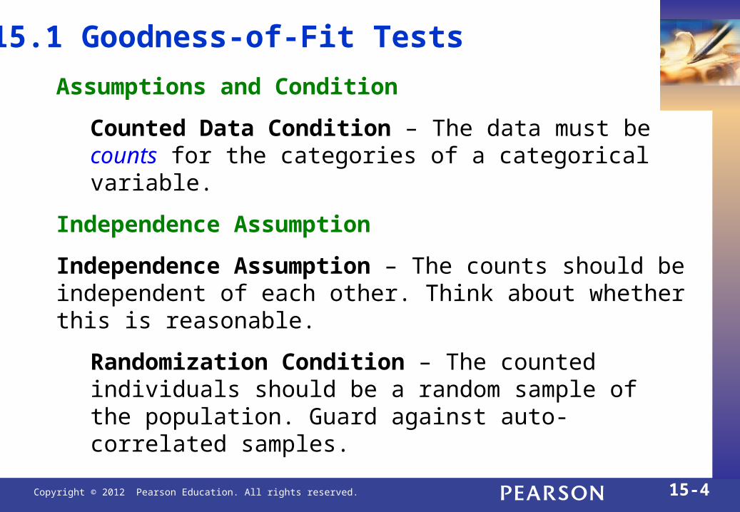
15.1 Goodness-of-Fit Tests
Assumptions and Condition
Counted Data Condition – The data must be counts for the categories of a categorical variable.
Independence Assumption
Independence Assumption – The counts should be independent of each other. Think about whether this is reasonable.
Randomization Condition – The counted individuals should be a random sample of the population. Guard against auto-correlated samples.

Copyright © 2012 Pearson Education. All rights reserved. 15-5
Sample Size Assumption
Sample Size Assumption -- There must be enough data so check the following condition.
Expected Cell Frequency Condition – Expect at least 5 individuals per cell.
15.1 Goodness-of-Fit Tests

Copyright © 2012 Pearson Education. All rights reserved. 15-6
15.1 Goodness-of-Fit TestsChi-Square Model
To decide if the null model is plausible, look at the differences between the observed values and the values expected if the model were true.
Note that “accumulates” the relative squared deviation of each cell from its expected value.
So, gets “big” when i) the data set is large and/or ii) the model is a poor fit.
2
2

Copyright © 2012 Pearson Education. All rights reserved. 15-7
15.1 Goodness-of-Fit TestsThe Chi-Square Calculation

Copyright © 2012 Pearson Education. All rights reserved. 15-8
15.1 Goodness-of-Fit TestsExample : Credit Cards
At a major credit card bank, the percentages of people who historically apply for the Silver, Gold, and Platinum cards are 60%, 30%, and 10% respectively. In a recent sample of customers, 110 applied for Silver, 55 for Gold, and 35 for Platinum. Is there evidence to suggest the percentages have changed?
What type of test do you conduct?
What are the expected values?
Find the test statistic and p-value.
State conclusions.

Copyright © 2012 Pearson Education. All rights reserved. 15-9
15.1 Goodness-of-Fit TestsExample : Credit Cards
At a major credit card bank, the percentages of people who historically apply for the Silver, Gold, and Platinum cards are 60%, 30%, and 10% respectively. In a recent sample of customers, 110 applied for Silver, 55 for Gold, and 35 for Platinum. Is there evidence to suggest the percentages have changed?
What type of test do you conduct? This is a goodness-of-fit test comparing a single sample to previous information (the null model).
What are the expected values?
Silver Gold Platinum
Observed 110 55 35
Expected 120 60 20

Copyright © 2012 Pearson Education. All rights reserved. 15-10
15.1 Goodness-of-Fit TestsExample : Credit Cards
At a major credit card bank, the percentages of people who historically apply for the Silver, Gold, and Platinum cards are 60%, 30%, and 10% respectively. In a recent sample of customers, 110 applied for Silver, 55 for Gold, and 35 for Platinum. Is there evidence to suggest the percentages have changed?
Find the test statistic and p-value. Using df = 2, the p-value < 0.005
State conclusions. Reject the null hypothesis. There is sufficient evidence customers are not applying for cards in the traditional proportions.
2
2
2 2 2110 120 55 60 35 20
120 60 2012.499
all cells
Obs Exp
Exp
Copyright © 2012 Pearson Education. All rights reserved. 15-11
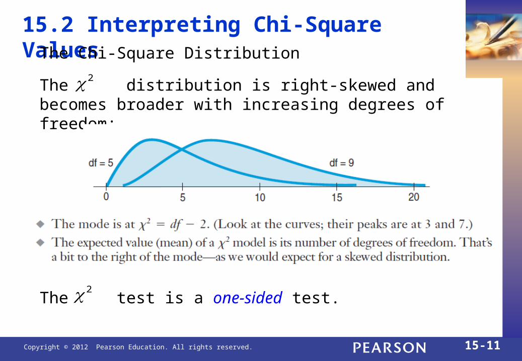
15.2 Interpreting Chi-Square ValuesThe Chi-Square Distribution
The distribution is right-skewed and becomes broader with increasing degrees of freedom:
2
The test is a one-sided test.2
Copyright © 2012 Pearson Education. All rights reserved. 15-12
15.2 Interpreting Chi-Square Values
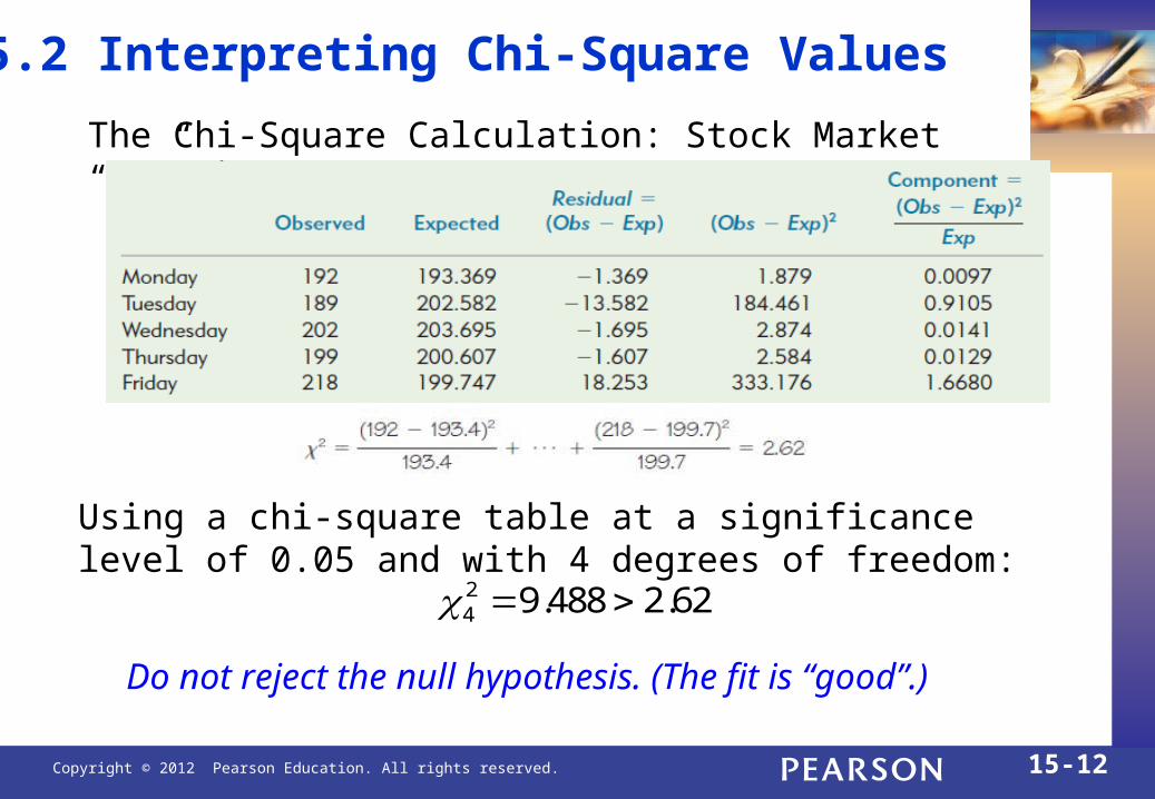
The Chi-Square Calculation: Stock Market “Up” Days
Using a chi-square table at a significance level of 0.05 and with 4 degrees of freedom:
24 9.488 2.62
Do not reject the null hypothesis. (The fit is “good”.)

Copyright © 2012 Pearson Education. All rights reserved. 15-13
When we reject a null hypothesis, we can examine the residuals in each cell to discover which values are extraordinary.
Because we might compare residuals for cells with very different counts, we should examine standardized residuals:
15.3 Examining the Residuals
Note that standardized residuals from goodness-of-fit tests are actually z-scores (which we already know how to interpret and analyze).

Copyright © 2012 Pearson Education. All rights reserved. 15-14
Standardized residuals for the trading days data:
15.3 Examining the Residuals
• None of these values is remarkable.
• The largest, Friday, at 1.292, is not impressive when viewed as a z-score.
• The deviations are in the direction of a “weekend effect”, but they aren’t quite large enough for us to conclude they are real.

Copyright © 2012 Pearson Education. All rights reserved. 15-15
Below are responses to the question, “How important is it to seek your utmost attractive appearance?”
15.4 The Chi-Square Test for Homogeneity

Copyright © 2012 Pearson Education. All rights reserved. 15-16
Convert the results to “column percentages”:
15.4 The Chi-Square Test for Homogeneity
Response patterns are beginning to become apparent.
Copyright © 2012 Pearson Education. All rights reserved. 15-17
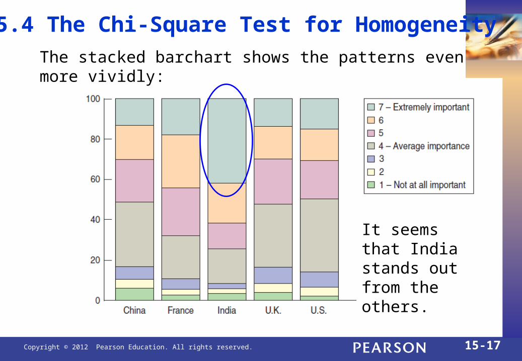
The stacked barchart shows the patterns even more vividly:
15.4 The Chi-Square Test for Homogeneity
It seems that India stands out from the others.

Copyright © 2012 Pearson Education. All rights reserved. 15-18
But, are the differences real or just natural sampling variation?
15.4 The Chi-Square Test for Homogeneity
Our null hypothesis is that the relative frequency distributions are the same (homogeneous) for each country.
Test the hypothesis with a chi-square test for homogeneity.

Copyright © 2012 Pearson Education. All rights reserved. 15-19
Use the Row % column to determine the expected counts for each table column (each country):
15.4 The Chi-Square Test for Homogeneity

Copyright © 2012 Pearson Education. All rights reserved. 15-20
Assumptions and Conditions
15.4 The Chi-Square Test for Homogeneity
Counted Data Condition – Data must be counts
Independence Assumption – Counts need to be independent from each other. Check for randomization
Randomization Condition – Random sample needed
Sample Size Assumption – There must be enough data so check the following condition.
Expected Cell Frequency Condition – Expect at least 5 individuals per cell.

Copyright © 2012 Pearson Education. All rights reserved. 15-21
Following the pattern of the goodness-of-fit test, compute the component for each cell:
15.4 The Chi-Square Test for Homogeneity
2
ComponentObs Exp
Exp
Then, sum the components:
2
2
all cells
Obs Exp
Exp
The degrees of freedom are 1 1 .R C
(The for the appearance survey indicates that the differences between countries are not due to random chance.)
2

Copyright © 2012 Pearson Education. All rights reserved. 15-22
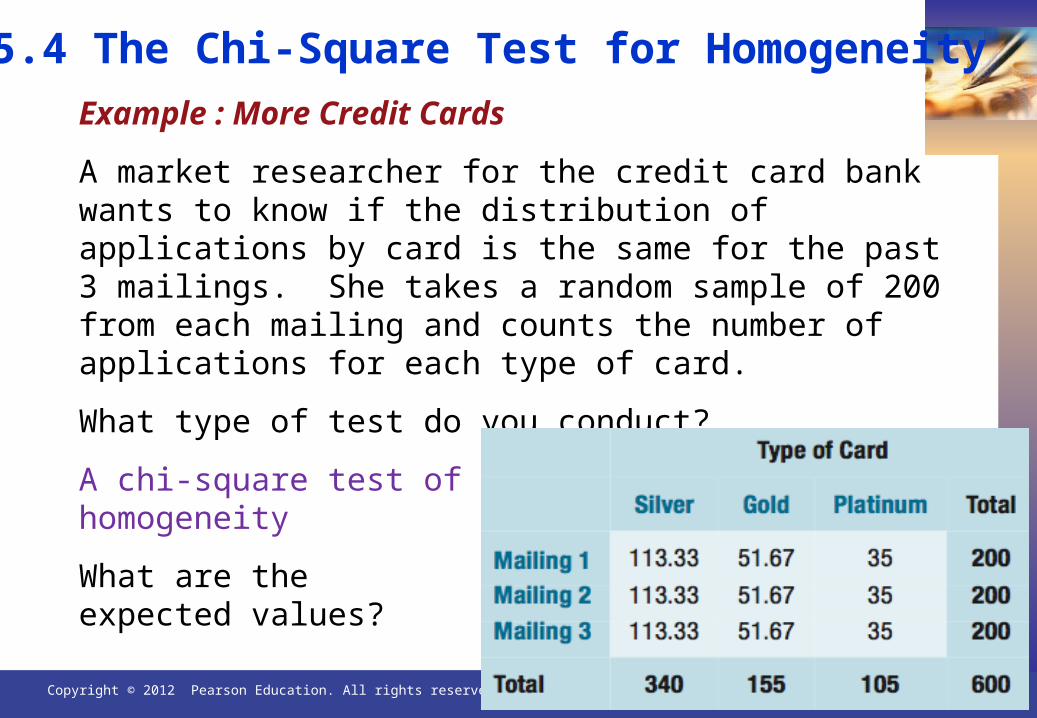
Example: More Credit Cards
A market researcher for the credit card bank wants to know if the distribution of applications by card is the same for the past 3 mailings. She takes a random sample of 200 from each mailing and counts the number of applications for each type of card.
What type of test do you conduct?
What are the expected values?
Find the test statistic and p-value.
State conclusions.
15.4 The Chi-Square Test for Homogeneity
Copyright © 2012 Pearson Education. All rights reserved. 15-23
Example : More Credit Cards
A market researcher for the credit card bank wants to know if the distribution of applications by card is the same for the past 3 mailings. She takes a random sample of 200 from each mailing and counts the number of applications for each type of card.
What type of test do you conduct?
A chi-square test ofhomogeneity
What are theexpected values?
15.4 The Chi-Square Test for Homogeneity

Copyright © 2012 Pearson Education. All rights reserved. 15-24
Example : More Credit Cards
A market researcher for the credit card bank wants to know if the distribution of applications by card is the same for the past 3 mailings. She takes a random sample of 200 from each mailing and counts the number of applications for each type of card.
Find the test statistic.
Given p-value > 0.10,state conclusions. Fail to reject the null. There is insufficient evidence to suggest that the distributions are different for the three mailings.
15.4 The Chi-Square Test for Homogeneity
2
2
2 2 2120 113.33 50 51.67 40 35
...113.33 51.67 35
2.7806
all cells
Obs Exp
Exp

Copyright © 2012 Pearson Education. All rights reserved. 15-25
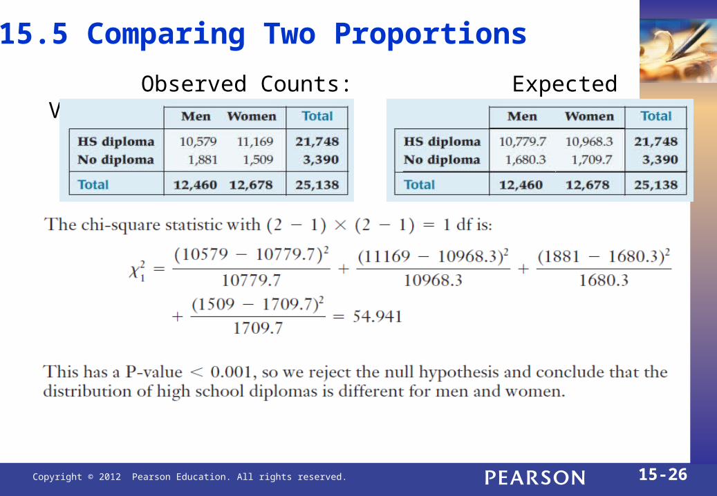
15.5 Comparing Two Proportions
Sample of 25,000 24-year-olds:
Men: 84.9% diploma rate
Women: 88.1% diploma rate
Are women more likely to graduate high school than men, or are the differences due to random variation?
Overall, of the sample had diplomas.
Use this proportion to compute the expected values.
2174886.5144%
25138
Copyright © 2012 Pearson Education. All rights reserved. 15-26
15.5 Comparing Two Proportions
Observed Counts: Expected Values:

Copyright © 2012 Pearson Education. All rights reserved. 15-27
15.5 Comparing Two Proportions

Copyright © 2012 Pearson Education. All rights reserved. 15-28
15.5 Comparing Two Proportions
Sample of 25,000 24-year-olds:
For high school graduation, a 95% confidence interval for the true difference between women’s and men’s rates is:
We can be 95% confident that women’s rates of having a HS diploma by 2000 were 2.36% to 4.04% higher than men’s.
1 2 2 21 2
1 2
ˆ ˆ ˆ ˆˆ ˆ( ) *
(0.881)(0.119) (0.849)(0.151)(0.881 0.849)
12678 2460(0.0236, 0.0404)
p q p qp p z
n n

Copyright © 2012 Pearson Education. All rights reserved. 15-29
15.6 Chi-Square Test of Independence
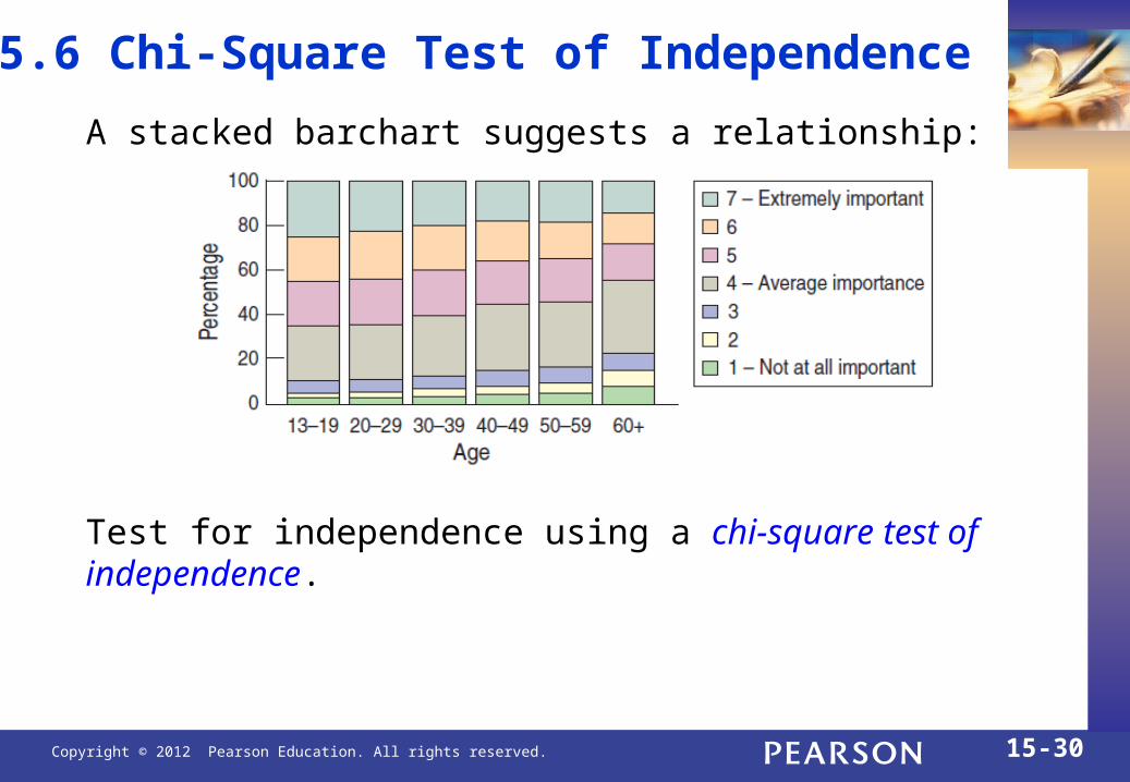
The table below shows the importance of personal appearance for several age groups.
Are Age and Appearance independent, or is there a relationship?
Copyright © 2012 Pearson Education. All rights reserved. 15-30
15.6 Chi-Square Test of Independence
A stacked barchart suggests a relationship:
Test for independence using a chi-square test of independence.

Copyright © 2012 Pearson Education. All rights reserved. 15-31
15.6 Chi-Square Test of Independence
The test is mechanically equivalent to the test for homogeneity, but with some differences in how we think about the data and the results:
•Homogeneity Test: one variable (Appearance) measured on two or more populations (countries).
•Independence Test: Two variables (Appearance and Age) measured on a single population.
We ask the question “Are the variables independent?” rather than “Are the groups homogeneous?” This subtle distinction is important when drawing conclusions.

Copyright © 2012 Pearson Education. All rights reserved. 15-32
Assumptions and Conditions
15.6 Chi-Square Test of Independence
Counted Data Condition – Data must be counts
Independence Assumption – Counts need to be independent from each other. Check for randomization
Randomization Condition – Random sample needed
Sample Size Assumption – There must be enough data so check the following condition.
Expected Cell Frequency Condition – Expect at least 5 individuals per cell.
Copyright © 2012 Pearson Education. All rights reserved. 15-33
15.6 Chi-Square Test of Independence
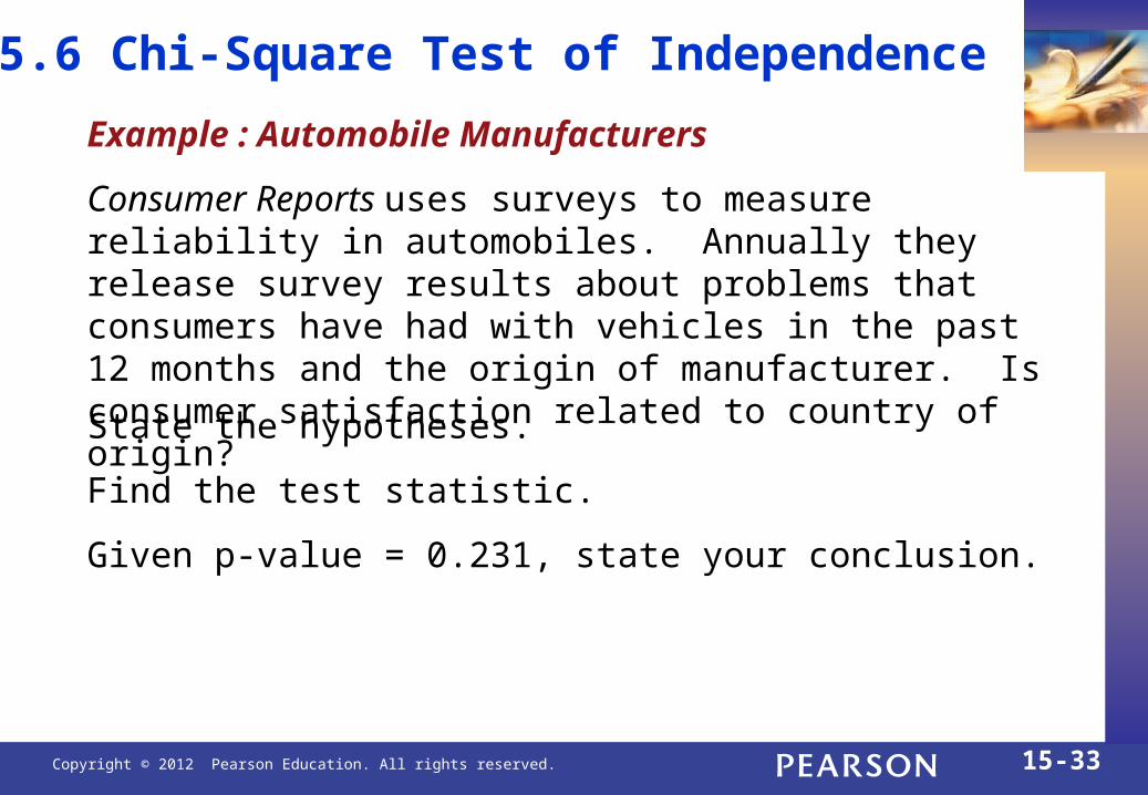
Example : Automobile Manufacturers
Consumer Reports uses surveys to measure reliability in automobiles. Annually they release survey results about problems that consumers have had with vehicles in the past 12 months and the origin of manufacturer. Is consumer satisfaction related to country of origin?
State the hypotheses.
Find the test statistic.
Given p-value = 0.231, state your conclusion.

Copyright © 2012 Pearson Education. All rights reserved. 15-34
15.6 Chi-Square Test of IndependenceExample : Automobile Manufacturers
Consumer Reports uses surveys to measure reliability in automobiles. Annually they release survey results about problems that consumers have had with vehicles in the past 12 months and the origin of manufacturer. Is consumer satisfaction related to country of origin?
State the hypotheses.
Find the test statistic.
Given p-value = 0.231, state your conclusion. There is not enough evidence to conclude there is an association between vehicle problems and origin of vehicle.
2 2 2
2 88 83.33 79 83.33 17 16.67...
83.33 83.33 16.67 2.928
o
a
H : Rate of problems is independent of manufacturer's origin
H : Rate of problems is not independent of manufacturer's origin

Copyright © 2012 Pearson Education. All rights reserved. 15-35
15.6 Chi-Square Test of Independence
For the Appearance and Age example, we reject the null hypothesis that the variables are independent.
So, it may be of interest to know how differently two age groups (teens and 30-something adults) select the “very important” category (Appearance response 6 or 7).
Construct a confidence interval for the true difference in proportions…

Copyright © 2012 Pearson Education. All rights reserved. 15-36
15.6 Chi-Square Test of Independence
From the data table, the percentage responses for Appearance = 6 or 7 are as follows:
Teens: 45.17%
30-39: 39.91%
The 95% confidence interval is found below:

Copyright © 2012 Pearson Education. All rights reserved. 15-37
Don’t use chi-square methods unless you have counts.
Beware large samples! With a sufficiently large sample size, a chi-square test can always reject the null hypothesis.
Don’t say that one variable “depends” on the other just because they’re not independent.

Copyright © 2012 Pearson Education. All rights reserved. 15-38
What Have We Learned?
Recognize when a chi-square test of goodness of fit, homogeneity, or independence is appropriate.
For each test, find the expected cell frequencies.
For each test, check the assumptions and corresponding conditions and know how to complete the test.
• Counted data condition.• Independence assumption; randomization makes independence more
plausible.• Sample size assumption with the expected cell frequency condition;
expect at least 5 observations in each cell.

Copyright © 2012 Pearson Education. All rights reserved. 15-39
What Have We Learned?
Interpret a chi-square test.• Even though we might believe the model, we cannot prove that the data
fit the model with a chi-square test because that would mean confirming the null hypothesis.
Examine the standardized residuals to understand what cells were responsible for rejecting a null hypothesis.

Copyright © 2012 Pearson Education. All rights reserved. 15-40
What Have We Learned?
Compare two proportions.
State the null hypothesis for a test of independence and understand how that is different from the null hypothesis for a test of homogeneity.
• Both are computed the same way. You may not find both offered by your technology. You can use either one as long as you interpret your result correctly.
Related Documents