Copyright © 2010 Pearson Prentice Hall. All rights reserved. Chapter 10 Cash Flow Estimation

Copyright © 2010 Pearson Prentice Hall. All rights reserved. Chapter 10 Cash Flow Estimation.
Dec 21, 2015
Welcome message from author
This document is posted to help you gain knowledge. Please leave a comment to let me know what you think about it! Share it to your friends and learn new things together.
Transcript
Copyright © 2010 Pearson Prentice Hall. All rights reserved.
Chapter 10
Cash Flow Estimation

Copyright © 2010 Pearson Prentice Hall. All rights reserved.10-2
Learning Objectives
1. Understand the importance of cash flow and the distinction between cash flow and profits.
2. Identify incremental cash flow.3. Calculate depreciation and cost recovery.4. Understand the cash flow associated with
the disposal of depreciable assets.5. Estimate incremental cash flow for capital
budgeting decisions.

Copyright © 2010 Pearson Prentice Hall. All rights reserved.10-3
10.1 The Importance of Cash Flow
Cash flow measures the actual inflow and outflow of cash, while profits represent merely an accounting measure of periodic performance.
A firm can spend its operating cash flow but not its net income.
Some firms have net losses (due to high depreciation write-offs) and yet can pay dividends from cash balances, while others show profits and may not have the cash available.
Thus, cash flow is broader than net income.
Copyright © 2010 Pearson Prentice Hall. All rights reserved.10-4
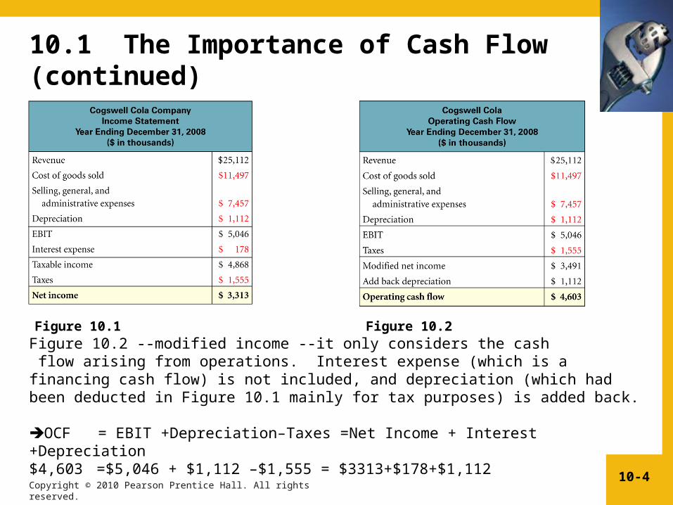
10.1 The Importance of Cash Flow (continued)
Figure 10.2 --modified income --it only considers the cash flow arising from operations. Interest expense (which is a financing cash flow) is not included, and depreciation (which had been deducted in Figure 10.1 mainly for tax purposes) is added back. OCF = EBIT +Depreciation–Taxes =Net Income + Interest +Depreciation$4,603 =$5,046 + $1,112 –$1,555 = $3313+$178+$1,112
Figure 10.1 Figure 10.2

Copyright © 2010 Pearson Prentice Hall. All rights reserved.10-5
10.2 Estimating Cash Flow for Projects: Incremental Cash Flow
• For expansion, replacement, or new project analysis, incremental effects on revenues and expenses must be considered.
• Careful estimation and evaluation of the timing and magnitude of incremental cash flows are very important.
• 7 important issues to be kept track of: • sunk costs• opportunity cost • erosion • synergy gains • working capital • capital expenditures• depreciation or cost recovery of assets
Copyright © 2010 Pearson Prentice Hall. All rights reserved.10-6
10.2 (A) Sunk costs
• Expenses that have already been incurred, or that will be incurred, regardless of the decision to accept or reject a project.
• For example, a marketing research study exploring business possibilities in a region would be a sunk cost, since its expenditure has taken place prior to undertaking the project and will have to be paid whether or not the project is taken on.
• These costs, although part of the income statement, should not be considered as part of the relevant cash flows when evaluating a capital budgeting proposal.

Copyright © 2010 Pearson Prentice Hall. All rights reserved.10-7
10.2 (B) Opportunity costs
• Costs that may not be directly observable or obvious, but result from benefits that are lost as a result of taking on a project.
• For example, if a firm decides to use an idle piece of equipment as part of a new business, the value of the equipment that could be realized by either selling or leasing it would be a relevant opportunity cost.
• These costs should be included.
Copyright © 2010 Pearson Prentice Hall. All rights reserved.10-8
10.2 (C) Erosion costs
• Costs that arise when a new product or service competes with revenue generated by a current product or service offered by a firm.
• For example, if a store offers two types of photocopying services--a newer, more expensive choice and an older economical one.
• Some of the revenues from the older repeat customers will be lost and should therefore be accounted for in the incremental cash flows.

Copyright © 2010 Pearson Prentice Hall. All rights reserved.10-9
10.2 (C) Erosion costs (continued)
Example 1: Erosion costsProblem Frosty Desserts currently sells 100,000 of its Strawberry
Shortcake Delight each year for $3.50 per serving. Its cost per serving is $1.75. Its chef has come up with a newer, richer concoction, “Extra-Creamy Strawberry Wonder,” which costs $2.00 per serving, will retail for $4.50 and should bring in 130,000 customers. It is estimated that after the launch, the sales for the original variety will drop by 15%. Estimate the erosion cost associated with this venture.
Copyright © 2010 Pearson Prentice Hall. All rights reserved.10-10
10.2 (C) Erosion costs (continued)
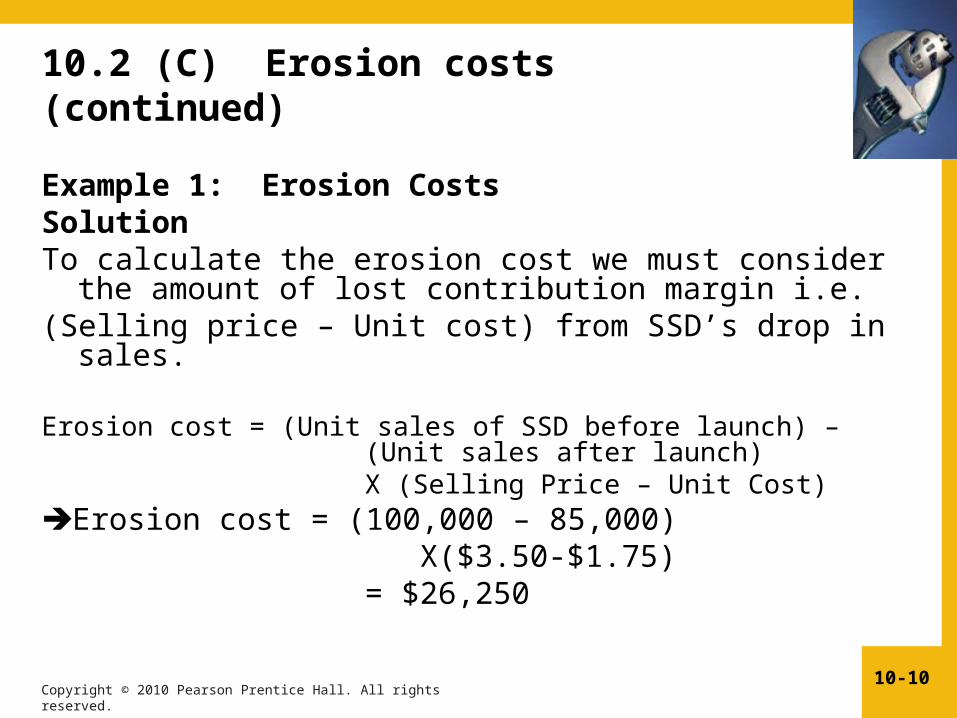
Example 1: Erosion CostsSolutionTo calculate the erosion cost we must consider the
amount of lost contribution margin i.e.(Selling price – Unit cost) from SSD’s drop in sales. Erosion cost = (Unit sales of SSD before launch) –
(Unit sales after launch) X (Selling Price – Unit Cost)
Erosion cost = (100,000 – 85,000) X($3.50-$1.75) = $26,250
Copyright © 2010 Pearson Prentice Hall. All rights reserved.10-11
10.2 (C) Erosion costs (continued)
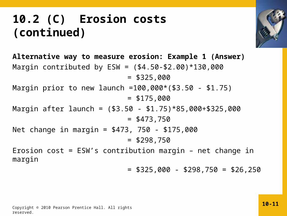
Alternative way to measure erosion: Example 1 (Answer)Margin contributed by ESW = ($4.50-$2.00)*130,000
= $325,000 Margin prior to new launch =100,000*($3.50 - $1.75)
= $175,000Margin after launch = ($3.50 - $1.75)*85,000+$325,000
= $473,750Net change in margin = $473, 750 - $175,000
= $298,750Erosion cost = ESW’s contribution margin – net change in margin
= $325,000 - $298,750 = $26,250
Copyright © 2010 Pearson Prentice Hall. All rights reserved.10-12
10.2 (D) Synergy gains
The increase in sales of an existing product due to the introduction of a new complementary product. For example, if a gas station with a convenience store attached adds a line of fresh donuts and bagels, the sales of coffee and milk would result in synergy gains.

Copyright © 2010 Pearson Prentice Hall. All rights reserved.10-13
10.2 (E) Working capital
• Additional cash flows arising from changes in current assets such as inventory and receivables (uses) and current liabilities such as accounts payables (sources) that occur as a result of a new project.
• Generally, at the end of the project, these additional cash flows are recovered and must be accordingly shown as cash inflows.
• Even though the net cash outflows--due to increase in net working capital at the start-- may equal the net cash inflow arising from the liquidation of the assets at the end, the time value of money effects make these costs relevant.
Copyright © 2010 Pearson Prentice Hall. All rights reserved.10-14
10.3 Capital Spending and Depreciation
Capital expenditures are allowed to be expensed on an annual basis and can be used as tax shields.
The portion written off in the income statement each year is called the depreciation expense; and the accumulated total kept track of in the balance sheet is known as Accumulated Depreciation.
Thus, the book value of an asset equals its original cost minus its accumulated depreciation.
Copyright © 2010 Pearson Prentice Hall. All rights reserved.10-15
10.3 Capital Spending and Depreciation (continued)
The two reasons we need to deal with depreciation when doing capital budgeting problems are:1) the tax-flow implications from the operating cash flow
and 2) the gain or loss at disposal of a capital asset.
Firms have a choice of using either straight line depreciation rates, or the modified accelerated cost recovery system (MACRS) rates for allocating the annual depreciation expense arising from an asset acquisition.
Copyright © 2010 Pearson Prentice Hall. All rights reserved.10-16
10.3 (A) Straight-line depreciation
• The annual depreciation expense is calculated by dividing the initial cost plus installation minus the expected residual value (at termination) equally over the expected productive life of the asset.
• The annual depreciation expenses are the same for each year.
Copyright © 2010 Pearson Prentice Hall. All rights reserved.10-17
10.3 (B) MACRS (Modified Accelerated Cost Recovery System)
• MACRS rates were established by the federal government in 1981 as a way to allow firms to accelerate the depreciation write-off in the early years of an asset’s life.
• These rates are set up based on various asset categories (class-lives).
Copyright © 2010 Pearson Prentice Hall. All rights reserved.10-18
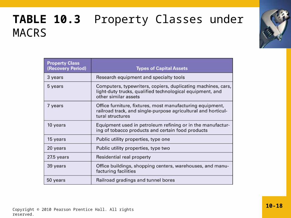
TABLE 10.3 Property Classes under MACRS
Copyright © 2010 Pearson Prentice Hall. All rights reserved.10-19
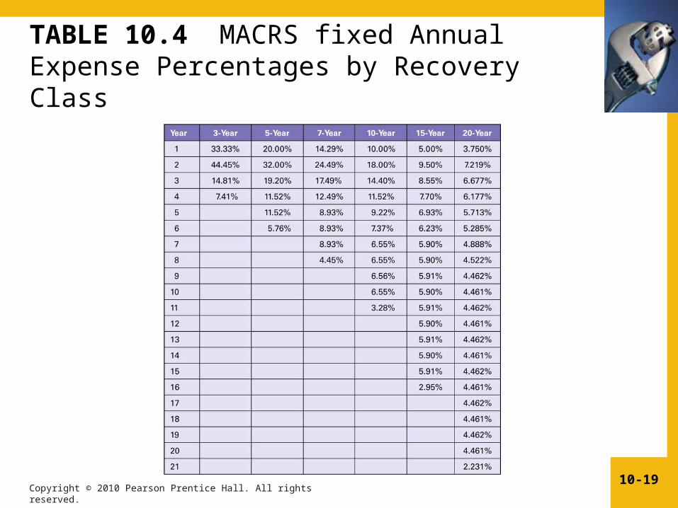
TABLE 10.4 MACRS fixed Annual Expense Percentages by Recovery Class

Copyright © 2010 Pearson Prentice Hall. All rights reserved.10-20
10.3 (B) MACRS (continued)
• Each class life appears to have one additional year of depreciation than the class-life states, e.g. a 3-year class life asset is depreciated over 4 years.
• What is actually happening is that the government assumes that the asset is put into use for only half a year at the start (half-year convention), and is thereby allowed ½ year of depreciation, with the last year (Year 4) also taking ½ year of depreciation.
• The depreciation rates in each column add up to 100%, i.e., there is no need to deduct residual value, with higher rates being allowed in earlier years and less in later years.
• With higher depreciation rates allowed in earlier years, the tax savings are higher due to the time value of money.
Copyright © 2010 Pearson Prentice Hall. All rights reserved.10-21
10.3 (B) MACRS (continued)
Example 2: MACRS DepreciationProblem The Grand Junction Furniture Company has
just bought some specialty tools to be used in the manufacture of high-end furniture. The cost of the equipment is $400,000 with an additional $30,000 for installation. If the company has a marginal tax rate of 30%, compute the annual tax savings that would be realized from using MACRS depreciation rates.

Copyright © 2010 Pearson Prentice Hall. All rights reserved.10-22
10.3 (B) MACRS (continued)
Example 2: MACRS DepreciationSolution
According to Table 10.3, specialty tools fall under a 3-year class asset, with rates in Years 1-4 of 33.33%, 44.45%, 14.81%, and 7.41% respectively.
Depreciable basis = Cost + Installation = $400,000 + $30,000 = $430,000
The annual depreciation expenses (i.e., annual rate*Dep. Basis)are shown below:
Year MACRS
rate Dep. Exp 1 33.33% $ 143,319 2 44.45% $ 191,135 3 14.81% $ 63,683 4 7.41% $ 31,863 Total 100.00% $ 430,000
Copyright © 2010 Pearson Prentice Hall. All rights reserved.10-23
10.4 Cash Flow and the Disposal of Capital Equipment
When a depreciable asset is sold, the cash inflow that results can be higher than, equal to, or lower than the actual selling price of the asset, depending on whether it was sold above (taxable gain), at (zero-gain) or below (tax credit) book value. If the sale results in a taxable gain, then the cash inflow is reduced by the amount of the taxes
i.e. (Tax rate*(Selling Price –Book Value). i.e. (Tax rate*(Selling Price –Book Value). If the selling price is exactly equal to book value, the cash inflow equals the sale price.
Copyright © 2010 Pearson Prentice Hall. All rights reserved.10-24
10.4 Cash Flow and the Disposal of Capital Equipment (continued)
If the asset is sold below its book value, a loss results, which can be written off in taxes for the year, effectively resulting in an addition to cash inflows equal to
(Book Value – Selling Price)*Tax rate(Book Value – Selling Price)*Tax rate.
Thus, the cash flow resulting from after-tax salvage value of a depreciable asset is calculated as follows:
After-tax Salvage Value = Selling Price – Tax rate * After-tax Salvage Value = Selling Price – Tax rate * (Selling price – Book Value)(Selling price – Book Value)
ORSelling Price + Tax rate * (Book Value – Selling Price)Selling Price + Tax rate * (Book Value – Selling Price)
Copyright © 2010 Pearson Prentice Hall. All rights reserved.10-25
10.4 Cash Flow and the Disposal of Capital Equipment (continued)
Example 3: Tax Effects from Disposal Cash FlowProblem Let’s say that the manager of the Grand Junction
Furniture Company decides to sell the specialty tools, acquired 2 years ago at a cost of $430,000 (including installation), to another firm for $125,000. How much of an after-tax cash flow will result? Assume that the tools were being depreciated based on the 3-year MACRS rates and that the company’s marginal tax rate is 35%.

Copyright © 2010 Pearson Prentice Hall. All rights reserved.10-26
10.4 Cash Flow and the Disposal of Capital Equipment (continued)
SolutionDepreciable basis = $430,000Year 1 depreciation rate = 33.33%Year 2 depreciation rate = 44.45% Total depreciation taken so far = $430,000 * (33.33% + 44.45%)
= $334, 454 Book Value = Depreciable basis – Accumulated depreciationBook Value = $430,000 - $334,454 = $95,546 Selling price = $125,000 > Book Value Taxable gain on the sale Taxable gain = $125,000-$95,546 = $29,454 After-tax Salvage Value= Selling Price – (Tax rate*Taxable gain ) =$125,000 - .35*($29,454) =$125,000-$10,308.9 =$114,691.1
Copyright © 2010 Pearson Prentice Hall. All rights reserved.10-27
10.5 Projected Cash Flow for a New Project
Four steps are typically involved:1. Determination of the initial capital
investment for the projectPurchase cost + Installation+Initial Increase in Net Working
Capital ––After––Tax Salvage Value from Disposal of Old Asset (if any)
Copyright © 2010 Pearson Prentice Hall. All rights reserved.10-28
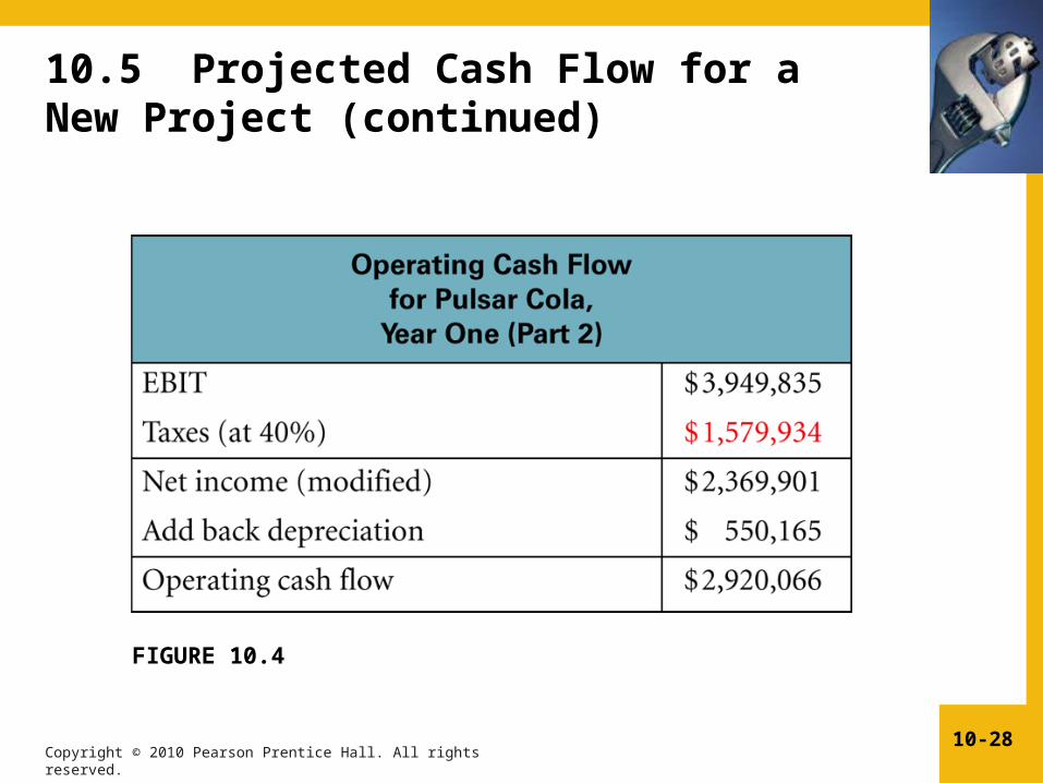
10.5 Projected Cash Flow for a New Project (continued)
FIGURE 10.4
Copyright © 2010 Pearson Prentice Hall. All rights reserved.10-29
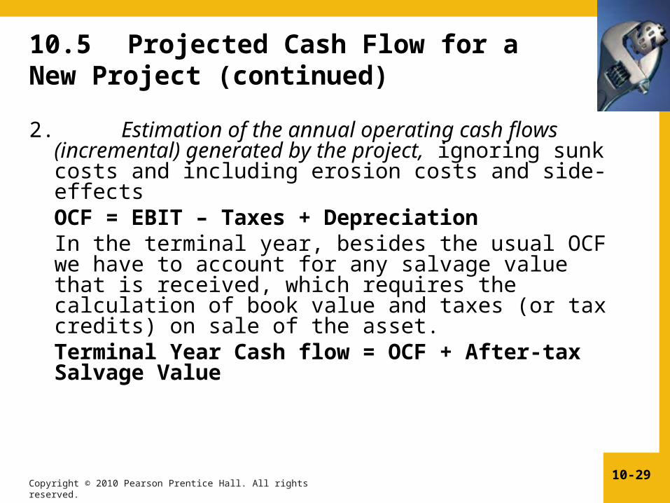
10.5 Projected Cash Flow for a New Project (continued)
2. Estimation of the annual operating cash flows (incremental) generated by the project, ignoring sunk costs and including erosion costs and side-effects OCF = EBIT – Taxes + Depreciation In the terminal year, besides the usual OCF we have to account for any salvage value that is received, which requires the calculation of book value and taxes (or tax credits) on sale of the asset.
Terminal Year Cash flow = OCF + After-tax Salvage Value
Copyright © 2010 Pearson Prentice Hall. All rights reserved.10-30
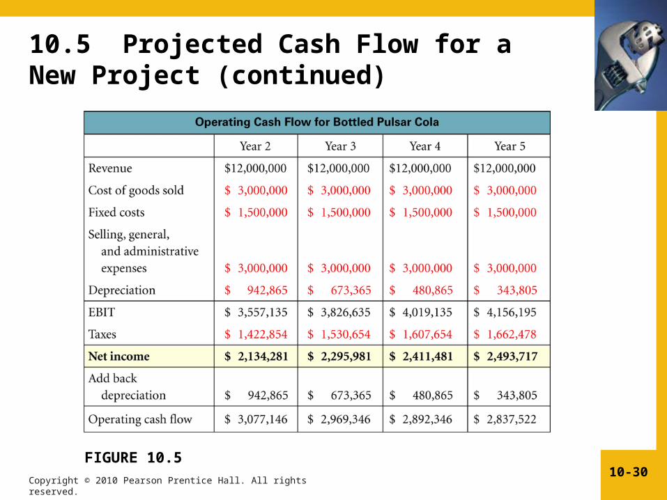
10.5 Projected Cash Flow for a New Project (continued)
FIGURE 10.5
Copyright © 2010 Pearson Prentice Hall. All rights reserved.10-31
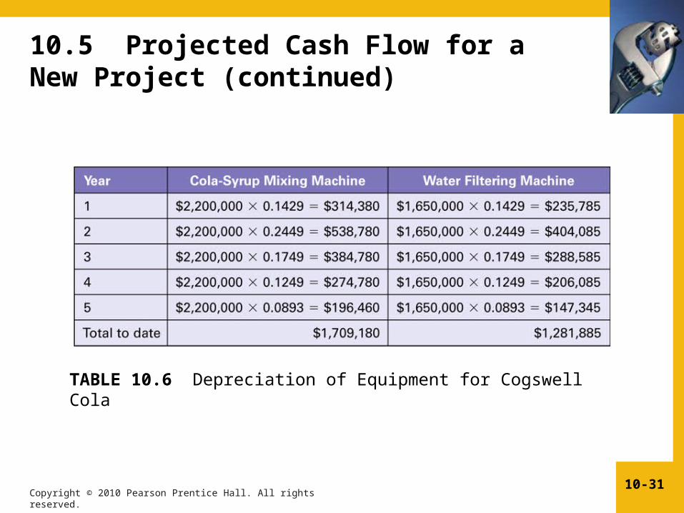
10.5 Projected Cash Flow for a New Project (continued)
TABLE 10.6 Depreciation of Equipment for Cogswell Cola
Copyright © 2010 Pearson Prentice Hall. All rights reserved.10-32
10.5 Projected Cash Flow for a New Project (continued)
3. Determination of the change in net working capital, which is usually an increase (outflow) at the beginning and a reduction (inflow) at the end
4. Evaluation of the proposed project using
an appropriate discount or hurdle rate and either the NPV or IRR approach
Copyright © 2010 Pearson Prentice Hall. All rights reserved.10-33
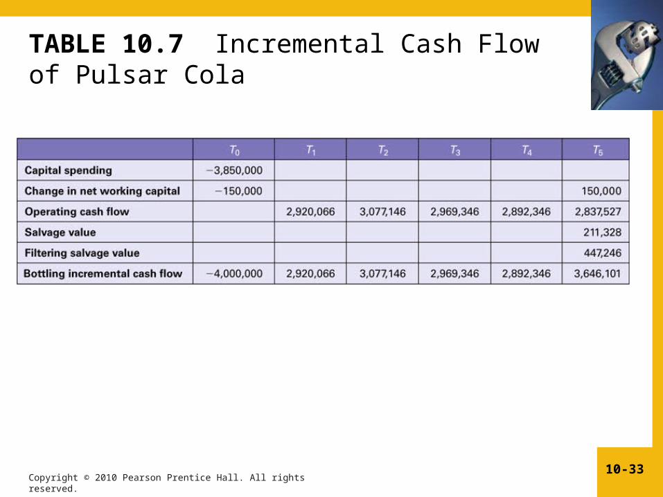
TABLE 10.7 Incremental Cash Flow of Pulsar Cola

Copyright © 2010 Pearson Prentice Hall. All rights reserved.10-34
Figure 10.6 Spreadsheet application for Pulsar Cola: calculating NPV, IRR, and MIRR
Copyright © 2010 Pearson Prentice Hall. All rights reserved.10-35
ADDITIONAL PROBLEMS WITH ANSWERSProblem 1
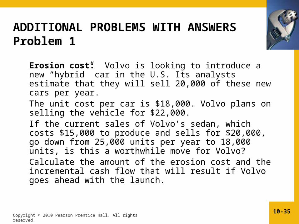
Erosion cost: Volvo is looking to introduce a new “hybrid” car in the U.S. Its analysts estimate that they will sell 20,000 of these new cars per year. The unit cost per car is $18,000. Volvo plans on selling the vehicle for $22,000. If the current sales of Volvo’s sedan, which costs $15,000 to produce and sells for $20,000, go down from 25,000 units per year to 18,000 units, is this a worthwhile move for Volvo? Calculate the amount of the erosion cost and the incremental cash flow that will result if Volvo goes ahead with the launch.

Copyright © 2010 Pearson Prentice Hall. All rights reserved.10-36
OLD SEDANCurrent EBIT = # of cars sold *(Price – Cost)
= 25,000*($20,000-$15,000) = $125,000,000= $125,000,000EBIT (after launch) = 18,000 *($5000) = $90,000,000
Lost EBIT = $125,000,000 - $90,000,000 = $35,000,000= Erosion Cost
HYBRIDEBIT = 20,000 * ($22,000-$18,000) = $80,000,000
COMBINED EBIT= $80,000,000 + $90,000,000 = $170,000,000$170,000,000 Since the Combined EBIT is higher than the current EBIT by $45,000,000, it would be a worthwhile move for Volvo.
ADDITIONAL PROBLEMS WITH ANSWERSProblem 1 (ANSWER)
Copyright © 2010 Pearson Prentice Hall. All rights reserved.10-37
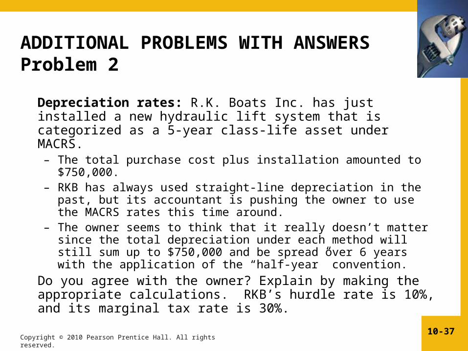
Depreciation rates: R.K. Boats Inc. has just installed a new hydraulic lift system that is categorized as a 5-year class-life asset under MACRS. – The total purchase cost plus installation amounted to $750,000.
– RKB has always used straight-line depreciation in the past, but
its accountant is pushing the owner to use the MACRS rates this time around.
– The owner seems to think that it really doesn’t matter since the total depreciation under each method will still sum up to $750,000 and be spread over 6 years with the application of the “half-year” convention.
Do you agree with the owner? Explain by making the appropriate calculations. RKB’s hurdle rate is 10%, and its marginal tax rate is 30%.
ADDITIONAL PROBLEMS WITH ANSWERSProblem 2

Copyright © 2010 Pearson Prentice Hall. All rights reserved.10-38
Under straight-line depreciation: Annual dep.exp. = Cost + Installation / Life = $750,000/5 = $150,000
Using the “half-year” convention, the comparison of yearly depreciation under the 2 methods is as follows:
ADDITIONAL PROBLEMS WITH ANSWERSProblem 2 (ANSWER)
Year MACRS
rate MACRS
Dep. St. Line
Dep Diff. Tax Gain
1 20% 150000 75,000 75,000 22500 2 32% 240000 150000 90,000 27000 3 19.20% 144000 150000 -6,000 -1800 4 11.52% 86400 150000 -63,600 -19080 5 11.52% 86400 150000 -63,600 -19080 6 5.76% 43200 75000 -31,800 -9540
Total 100% 750000 750000 0 0
NPV @10%
$2,265.82
So clearly, with the tax advantages coming in earlier, i.e., in the first two years, the time value of money advantages makes it a positive NPV move.
Copyright © 2010 Pearson Prentice Hall. All rights reserved.10-39
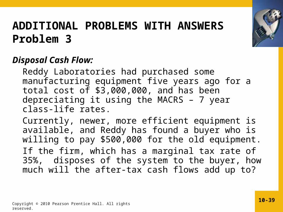
ADDITIONAL PROBLEMS WITH ANSWERSProblem 3Disposal Cash Flow: Reddy Laboratories had purchased some
manufacturing equipment five years ago for a total cost of $3,000,000, and has been depreciating it using the MACRS – 7 year class-life rates. Currently, newer, more efficient equipment is available, and Reddy has found a buyer who is willing to pay $500,000 for the old equipment. If the firm, which has a marginal tax rate of 35%, disposes of the system to the buyer, how much will the after-tax cash flows add up to?

Copyright © 2010 Pearson Prentice Hall. All rights reserved.10-40
ADDITIONAL PROBLEMS WITH ANSWERSProblem 3 (Answer)
After 5 years, the book value would be (0893+.0893+.0445)*$3,000,000Book value = 0.2231*$3,000,000 = $669, 300Loss on sale = Selling Price – Book value = $500,000 - $669,30
= -$169,300Tax credit = Tax rate * Loss = 0.35*$169,300 = $59,255After-tax cash inflow = Selling price + Tax credit
= $500,000 + $59,255 = $559,255
The 7-year MACRS rates are as follows:

Copyright © 2010 Pearson Prentice Hall. All rights reserved.10-41
Operating cash flow (growing each year; MACRS). Balik Ventures is looking at a project with the following forecasted sales: first-year sales quantity of 20,000 with an annual growth rate of 4% over the next 5 years. – the sales price per unit is $35.00 and will grow at 5% per year. – The production costs are expected to be 45% of the current year’s
sales price. – The manufacturing equipment to aid this project will have a total cost
(including installation) of $2,200,000. – It will be depreciated using MACRS and has a five-year
MACRS life classification. – Fixed costs are $285,000 per year. The firm has a tax rate of 35%.
What is the operating cash flow for this project over these 5 years? Hint: Use a spreadsheet and round units to the nearest whole number.
ADDITIONAL PROBLEMS WITH ANSWERSProblem 4
Copyright © 2010 Pearson Prentice Hall. All rights reserved.10-42
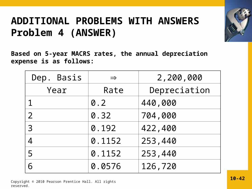
ADDITIONAL PROBLEMS WITH ANSWERSProblem 4 (ANSWER)Based on 5-year MACRS rates, the annual depreciation expense is as follows:
Dep. Basis 2,200,000
Year Rate Depreciation
1 0.2 440,000
2 0.32 704,000
3 0.192 422,400
4 0.1152 253,440
5 0.1152 253,440
6 0.0576 126,720

Copyright © 2010 Pearson Prentice Hall. All rights reserved.10-43
ADDITIONAL PROBLEMS WITH ANSWERSProblem 4 (ANSWER)The operating cash flow over the 5-year period is calculated as follows:
Rate Year 1 Year 2 Year 3 Year 4 Year 5
Unit sales 4% 30,000 31,200 32,448 33,746 35,096 Sales price 5% $35.00 $36.75 $38.59 $40.52 $42.54 Revenues
$1,050,000 $1,146,600 $1,252,087 $1,367,279 $1,493,069
Prod. Costs 45% $472,500 $515,970 $563,439 $615,276 $671,881 Fixed costs
$ 285,000 $ 285,000 $ 285,000 $ 285,000 $ 285,000
Depreciation
$440,000 $704,000 $422,400 $253,440 $253,440 EBIT
($147,500) ($358,370) ($18,752) $213,564 $282,748
Taxes 35% ($51,625) ($125,430) ($6,563) $74,747 $98,962 Net Income
($95,875) ($232,941) ($12,189) $138,816 $183,786
Add Dep
$440,000 $704,000 $422,400 $253,440 $253,440 Op. Cash Flow $344,125 $471,060 $410,211 $392,256 $437,226
Copyright © 2010 Pearson Prentice Hall. All rights reserved.10-44
ADDITIONAL PROBLEMS WITH ANSWERSProblem 5
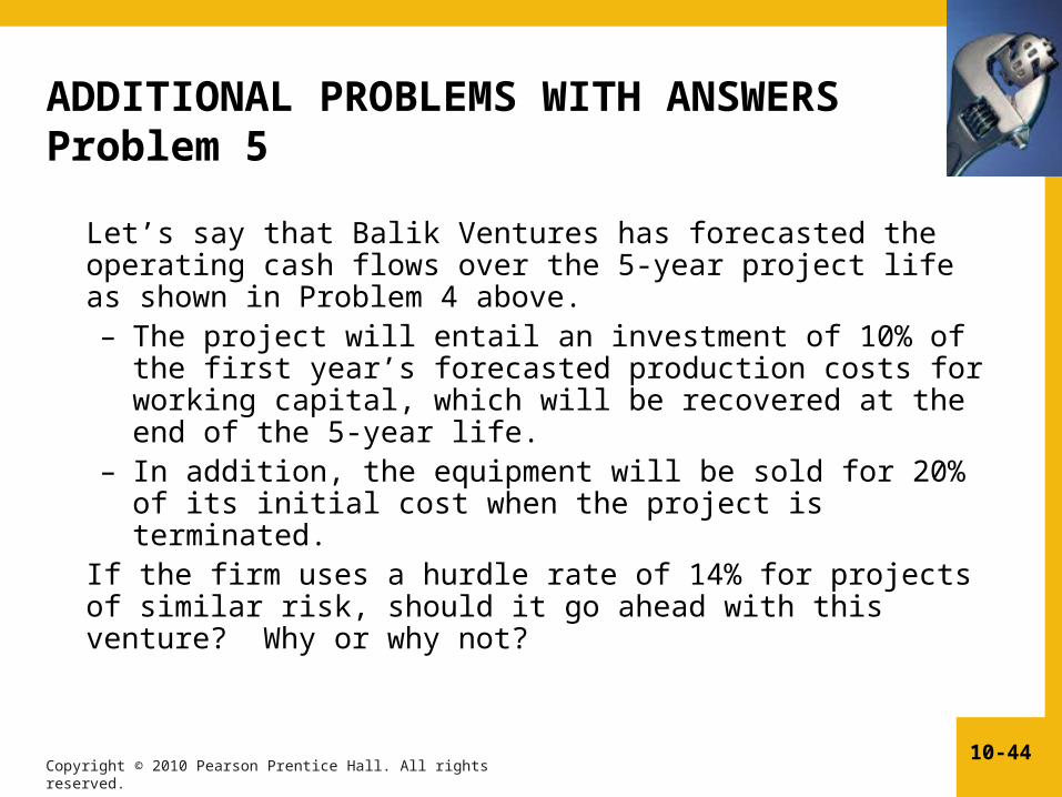
Let’s say that Balik Ventures has forecasted the operating cash flows over the 5-year project life as shown in Problem 4 above. – The project will entail an investment of 10% of the first
year’s forecasted production costs for working capital, which will be recovered at the end of the 5-year life.
– In addition, the equipment will be sold for 20% of its initial cost when the project is terminated.
If the firm uses a hurdle rate of 14% for projects of similar risk, should it go ahead with this venture? Why or why not?
Copyright © 2010 Pearson Prentice Hall. All rights reserved.10-45
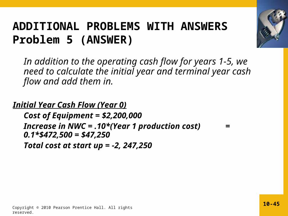
ADDITIONAL PROBLEMS WITH ANSWERSProblem 5 (ANSWER)
In addition to the operating cash flow for years 1-5, we need to calculate the initial year and terminal year cash flow and add them in.
Initial Year Cash Flow (Year 0)
Cost of Equipment = $2,200,000Increase in NWC = .10*(Year 1 production cost) = 0.1*$472,500 = $47,250Total cost at start up = -2, 247,250
Copyright © 2010 Pearson Prentice Hall. All rights reserved.10-46
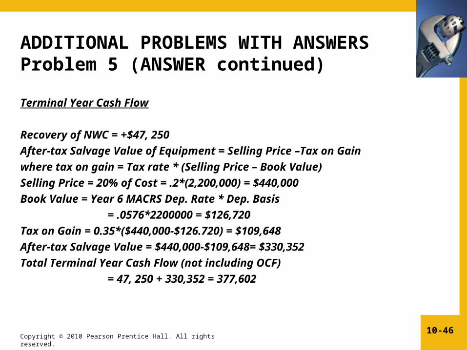
ADDITIONAL PROBLEMS WITH ANSWERSProblem 5 (ANSWER continued)Terminal Year Cash Flow Recovery of NWC = +$47, 250After-tax Salvage Value of Equipment = Selling Price –Tax on Gainwhere tax on gain = Tax rate * (Selling Price – Book Value)Selling Price = 20% of Cost = .2*(2,200,000) = $440,000Book Value = Year 6 MACRS Dep. Rate * Dep. Basis
= .0576*2200000 = $126,720Tax on Gain = 0.35*($440,000-$126.720) = $109,648After-tax Salvage Value = $440,000-$109,648= $330,352 Total Terminal Year Cash Flow (not including OCF)
= 47, 250 + 330,352 = 377,602

Copyright © 2010 Pearson Prentice Hall. All rights reserved.10-47
ADDITIONAL PROBLEMS WITH ANSWERSProblem 5 (ANSWER continued)
Year Cash Flow 0 -$2,247,250 1 $344,125 2 $471,060 3 $410,211 4 $392,256 5 $437,226+377,602=$814,828
NPV @10% = -$463,045.5 REJECT THE PROJECT!

Copyright © 2010 Pearson Prentice Hall. All rights reserved.10-48
TABLE 10.1 Annual Incremental Cash Revenues
Copyright © 2010 Pearson Prentice Hall. All rights reserved.10-49
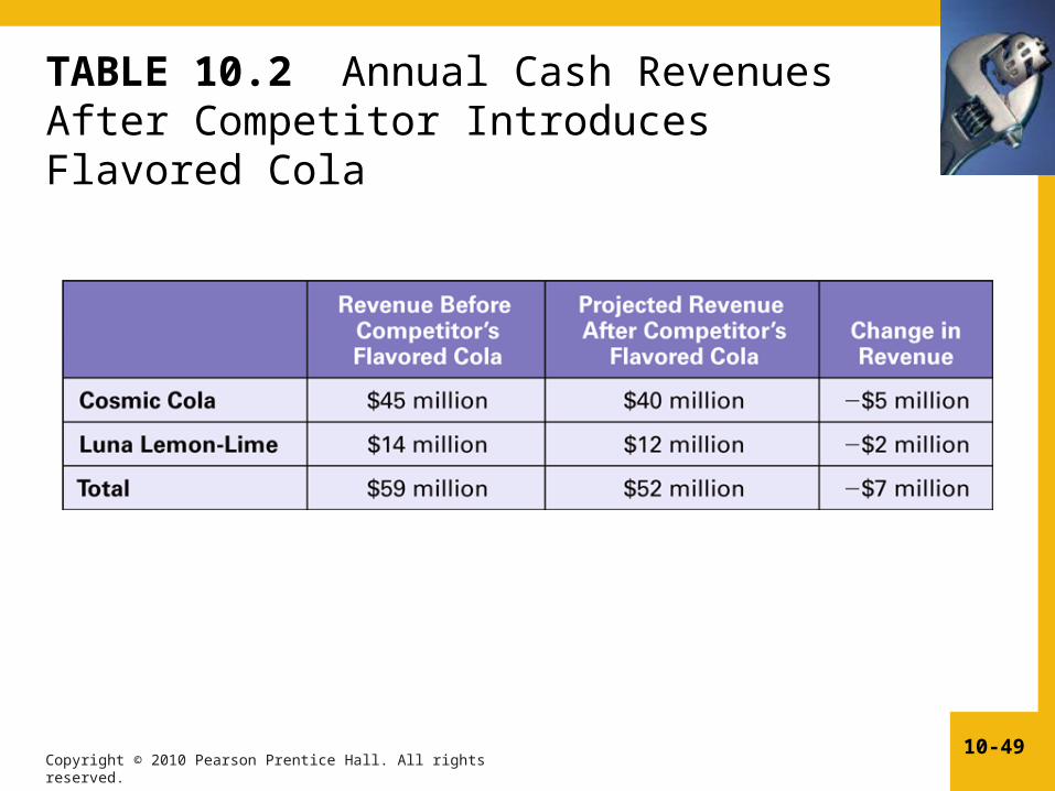
TABLE 10.2 Annual Cash Revenues After Competitor Introduces Flavored Cola

Copyright © 2010 Pearson Prentice Hall. All rights reserved.10-50
TABLE 10.5 Annual Depreciation Expense of Equipment for Cogswell Cola
Copyright © 2010 Pearson Prentice Hall. All rights reserved.10-51
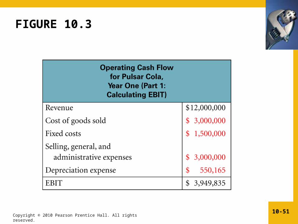
FIGURE 10.3
Related Documents