Copyright © 2009 PMI RiskSIGNovember 5-6, 2009 RiskSIG - Advancing the State of the Art A collaboration of the PMI, Rome Italy Chapter and the RiskSIG.

Copyright © 2009 PMI RiskSIGNovember 5-6, 2009

RiskSIG - Advancing the State of the ArtRiskSIG - Advancing the State of the Art

A collaboration of theA collaboration of the PMI, Rome Italy Chapter PMI, Rome Italy Chapter

and the RiskSIGand the RiskSIG

““Project Risk Management – Project Risk Management – An International An International

Perspective”Perspective”

Copyright © 2009 PMI RiskSIG Slide 2November 5-6, 2009

Bayesian Networks:

A Novel Approach

For Modelling Uncertainty in Projects

By: Vahid Khodakarami


Outline:

What is missing in current PRM practice? Bayesian Networks Application of BNs in PRM Models Case study


Conceptual steps in PRMP

Risk IdentificationQualitative Analysis

Risk Analysis (Risk Measurement)Quantitative Analysis

Risk Response (Mitigation)


Project Scheduling Under uncertainty

(CPM) PERT Simulation Critical chain


What is missing?

Causality in project uncertainty Estimation and Subjectivity Unknown Risks (Common cause factors) Trade-off between time, cost and

performance Dynamic Learning


Bayesian Networks (BNs)

Graphical modelNodes (variables)Arcs (causality)

Probabilistic (Bayesian) inference


Bayesian vs. Frequentist

Frequentist Bayesian

Variables Random Uncertain

Probability

Physical Property

(Data)

Degree of belief (Subjective)

Inference Confidence interval

Bayes’ Theorem

only feasible

method for many

practical problems


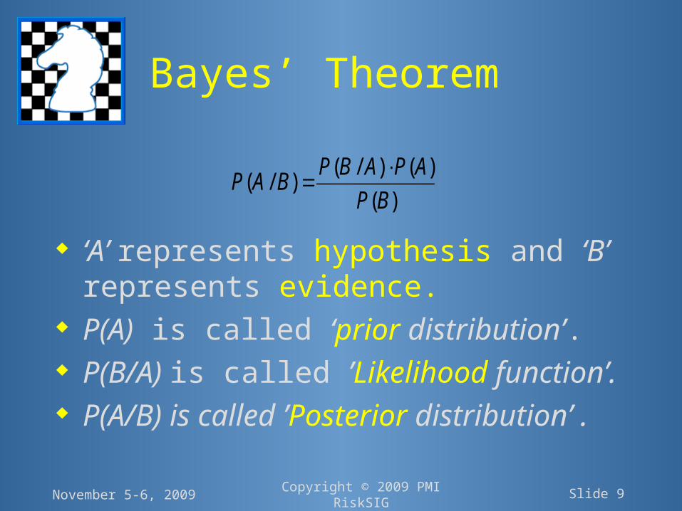
Bayes’ Theorem

‘A’ represents hypothesis and ‘B’ represents evidence.

P(A) is called ‘prior distribution’. P(B/A) is called ’Likelihood function’. P(A/B) is called ’Posterior distribution’ .

( / ) ( )( / )

( )

P B A P AP A B

P B


Constructing BN

High 0.7

Low 0.3

On time 0.95

Late 0.05

Prior Probability

Sub-contract On time Late

Staff Experience High Low High Low No 0.99 0.8 0.7 0.02Delay Yes 0.01 0.2 0.3 0.98

Conditional Probability


Inference in BN(cause to effect)

With no other information

P(Delay)=0.14.4

Knowing the sub-contract is late

P(Delay)=0.50.7


Backward Propagation(effect to cause)

Prior probability with no data

(0.7,0.3)

Posterior (learnt) probability

(0.28,0.72)


BNs Advantages

Rigorous method to make formal use of subjective data Explicitly quantify uncertainty Make predictions with incomplete data Reason from effect to cause as well as from cause to effect Update previous beliefs in the light of new data (learning) Complex sensitivity analysis


BNs Applications

Industrial Processor Fault Diagnosis - by

Intel Auxiliary Turbine Diagnosis -

by GE Diagnosis of space shuttle

propulsion systems - by NASA/Rockwell

Situation assessment for nuclear power plant – NRC

Medical Diagnosis Internal Medicine Pathology diagnosis - Breast Cancer Manager

Commercial Software troubleshooting and

advice – MS-Office Financial Market Analysis Information Retrieval Software Defect detection

Military Automatic Target Recognition

– MITRE Autonomous control of

unmanned underwater vehicle - Lockheed Martin


Bayesian CPM

ES

D

EFLF

LS

PredecessorActivities

SuccessorActivities

Su

ccesso

rs

Pred

ecesso

rs

Duration Model

CPM Calculation[ j ]jES Max EF one of the predecessor activities |

EF ES D

LS LF D

[ j ]jLF Min LS one of the successor activities | Slack LS ES LF EF


BCPM Example

D=5 EF=5

LS=0 Slack=0 LF=5

ES=0

A

D=4 EF=9

LS=9 Slack=4 LF=13

ES=5

B

D=10 EF=15

LS=5 Slack=0 LF=15

ES=5

C

D=2 EF=11

LS=13 Slack=4 LF=15

ES=9

D

D=5 EF=20

LS=15 Slack=0 LF=20

ES=15

E


Activity Duration


Trade off


Trade off (Prior vs. required resources )


Known Risk


Known Risk (Control)


Known Risk (Impact)


Known Risk (Response)


Unknown Factors


Unknown Factors (Learning)


Learnt distribution


Total Duration


Case Study (construction Project)


Case Study (Bayesian CPM)


Case Study (predictive)


Case Study (diagnostic)


Case Study (learning)


Summary

Current practice in modelling risk in project time management has serious limitations

BNs are particularly suitable for modelling uncertainty in project

The proposed models provide a new generation of project risk assessment tools that are better informed and hence, more valid


Questions?

Thank you for your attention

Copyright © 2009 PMI RiskSIGNovember 5-6, 2009 RiskSIG - Advancing the State of the Art A collaboration of the PMI, Rome Italy Chapter and the RiskSIG.

Documents