Copyright © 2009 Pearson Education, Inc. 10.2 LEARNING GOAL Interpret and carry out hypothesis tests for independence of variables with data organized.

Copyright © 2009 Pearson Education, Inc.

10.2

LEARNING GOAL

Interpret and carry out hypothesis tests for independence of variables with data organized in two-way tables.

Hypothesis Testing with Two-Way Tables

Slide 10.2- 2Copyright © 2009 Pearson Education, Inc.

Identifying the Hypotheses with Two Variables

Suppose that administrators at a college are concerned that there may be bias in the way degrees are awarded to men and women in different departments. They therefore collect data on the number of degrees awarded to men and women in different departments.

These data concern two variables: major and gender.

To test whether there is bias in the awarding of degrees, the administrators ask the following question:

Do the data suggest a relationship between the two variables?

Slide 10.2- 3Copyright © 2009 Pearson Education, Inc.

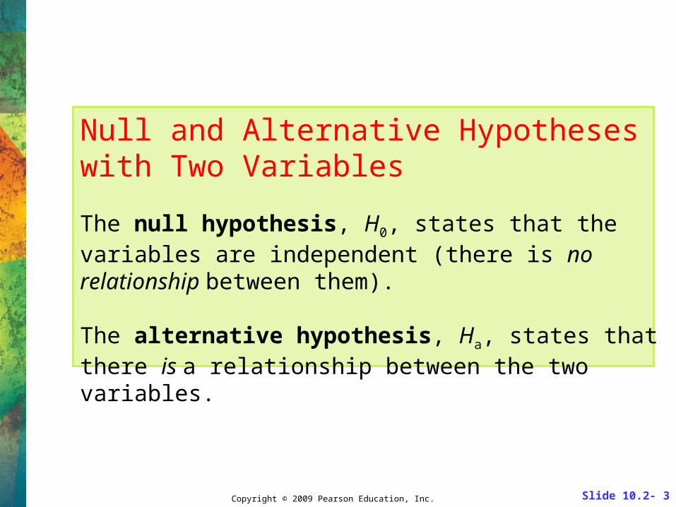
Null and Alternative Hypotheses with Two Variables

The null hypothesis, H0, states that the variables are independent (there is no relationship between them).

The alternative hypothesis, Ha, states that there is a relationship between the two variables.

Slide 10.2- 4Copyright © 2009 Pearson Education, Inc.

Displaying the Data in Two-Way Tables

With the hypotheses identified, the next step in the hypothesis test is to examine the data set to see if it supports rejecting or not rejecting the null hypothesis.

We can display the data efficiently with a two-way table (also called a contingency table), so named because it displays two variables.

Slide 10.2- 5Copyright © 2009 Pearson Education, Inc.

Note: One variable is displayed along the columns and the other along the rows. Here, there are only two rows because gender can be only either male or female. There are many columns for the majors, with just the first few shown here.

Slide 10.2- 6Copyright © 2009 Pearson Education, Inc.

Two-Way TablesA two-way table shows the relationship between two variables by listing one variable in the rows and the other variable in the columns.

The entries in the table’s cells are called frequencies (or counts).

Slide 10.2- 7Copyright © 2009 Pearson Education, Inc.

Here, to simplify the calculations, let’s focus on just twomajors, biology and business.

Does a person’s gender influence whether he or she chooses to major in biology or business?

Table 10.3 shows the biology and business data extracted from Table 10.2, along with row and column totals.

Slide 10.2- 8Copyright © 2009 Pearson Education, Inc.

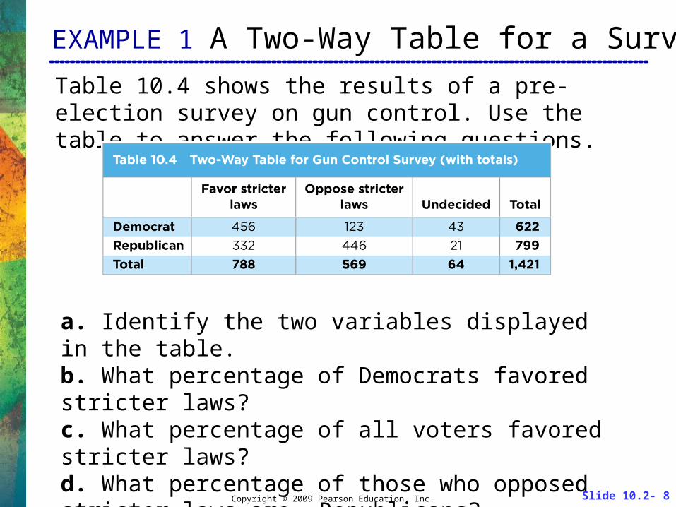
Table 10.4 shows the results of a pre-election survey on gun control. Use the table to answer the following questions.

a. Identify the two variables displayed in the table.b. What percentage of Democrats favored stricter laws?c. What percentage of all voters favored stricter laws?d. What percentage of those who opposed stricter laws are Republicans?

EXAMPLE 1 A Two-Way Table for a Survey

Slide 10.2- 9Copyright © 2009 Pearson Education, Inc.

Note that the total of the row totals and the total of the column totals are equal.a. The rows show the variable survey response, which can be either “favor stricter laws,” “oppose stricter laws,” or “undecided.” The columns show the variable party affiliation,which in this table can be either Democrat or Republican.b. Of the 622 Democrats polled, 456 favored stricter laws. The percentage of Democrats favoring stricter laws is 456/622 = 0.733, or 73.3%.

EXAMPLE 1 A Two-Way Table for a Survey

Solution:

Slide 10.2- 10Copyright © 2009 Pearson Education, Inc.

c. Of the 1,421 people polled, 788 favored stricter laws. The percentage of all respondents favoring stricter laws is 788/1,421 = 0.555, or 55.5%.d. Of the 569 people polled who opposed stricter laws, 446 are Republicans. Since 446/569 = 0.783, 78.3% of those opposed to stricter laws are Republicans.

EXAMPLE 1 A Two-Way Table for a Survey

Solution: (cont.)

Slide 10.2- 11Copyright © 2009 Pearson Education, Inc.

Carrying Out the Hypothesis TestThe basic idea of the hypothesis test is the same as always—to decide whether the data provide enough evidence to reject the null hypothesis.

For the case of a test with a two-way table, the specific steps are as follows:

• As always, we start by assuming that the null hypothesis is true, meaning there is no relationship between the two variables. In that case, we would expect the frequencies (the numbers in the individual cells) in the two-way table to be those that would occur by pure chance.

Our first step, then, is to find a way to calculate the frequencies we would expect by chance.

Slide 10.2- 12Copyright © 2009 Pearson Education, Inc.

• We next compare the frequencies expected by chance to the observed frequencies from the sample, which are the frequencies displayed in the table.

We do this by calculating something called the chi-square statistic (pronounced “ky-square”) for the sample data, which here plays a role similar to the role of the standard score z in the hypothesis tests we carried out in Chapter 9 or the role of the t test statistic in Section 10.1.

Carrying Out the Hypothesis Test(cont.)

Slide 10.2- 13Copyright © 2009 Pearson Education, Inc.

• Recall that for the hypothesis tests in Chapter 9, we made the decision about whether to reject or not reject the null hypothesis by comparing the computed value of the standard score for the sample data to critical values given in tables; similarly, in Section 10.1 we compared computed values of the t test statistic to values found in a table.

Here, we do the same thing, except rather than using critical values for the standard score or t, we use critical values for the chi-square statistic.

Carrying Out the Hypothesis Test(cont.)

Slide 10.2- 14Copyright © 2009 Pearson Education, Inc.

As an example of the process, let’s work through these steps with the data in Table 10.3.

Our first step is to find the frequencies we would expect in Table 10.3 if there were no relationship between the variables, which is equivalent to the frequency expected by chance alone.

Let’s start by finding the frequency we would expect by chance for male business majors.

Finding the Frequencies Expected by Chance

Carrying Out the Hypothesis Test

Slide 10.2- 15Copyright © 2009 Pearson Education, Inc.

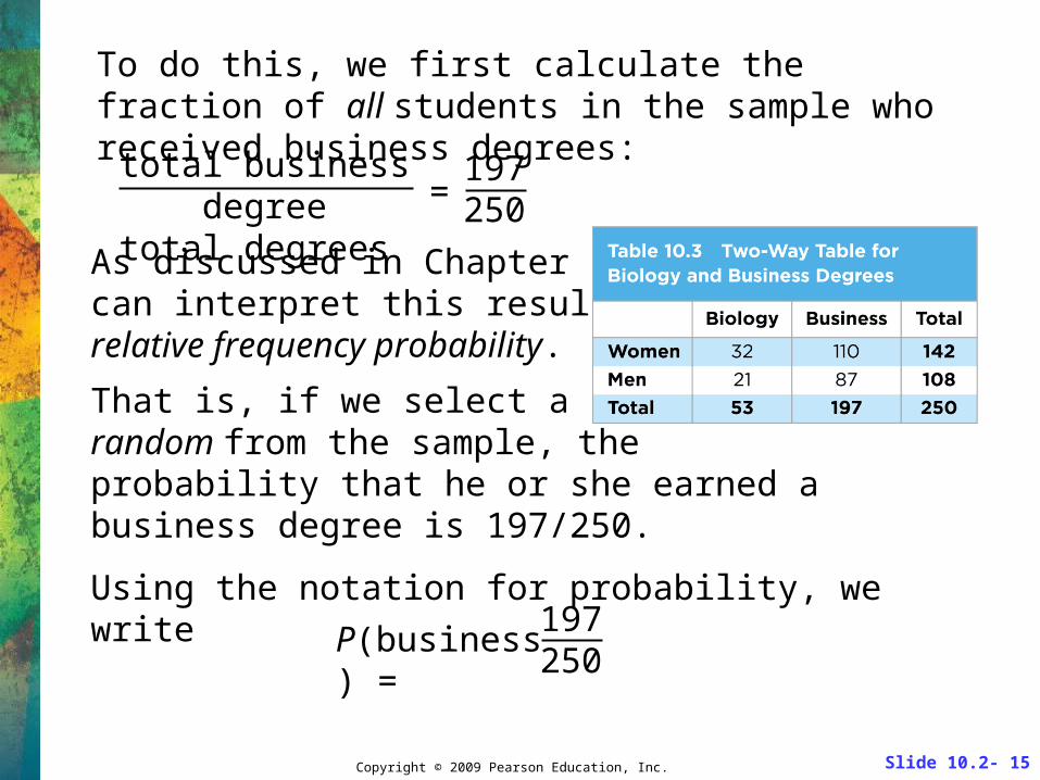
197250

P(business) =

As discussed in Chapter 6, we can interpret this result as a relative frequency probability.

That is, if we select a student at random from the sample, the probability that he or she earned a business degree is 197/250.

Using the notation for probability, we write

To do this, we first calculate the fraction of all students in the sample who received business degrees:

total business degreetotal degrees

197250=

Slide 10.2- 16Copyright © 2009 Pearson Education, Inc.

Recall from Section 6.5 that if two events A and B are independent (the outcome of one does not affect the probability of the other), then

We can apply this rule to determine the probability that a student is both a man and a business major (assuming the null hypothesis that gender is independent of major):

P(man and business) =

P(A and B) = P(A) × P(B)

108250

P(man) × P(business) = × ≈ 0.3404197250

Similarly, if we select a student at random from the sample, the probability that this student is a man is

108250

P(man) =

Slide 10.2- 17Copyright © 2009 Pearson Education, Inc.

This probability is equivalent to the fraction of the total students whom we expect to be male business majors if there is no relationship between gender and major.

108250 × × 250 ≈ 85.104

197250

We therefore multiply this probability by the total number of students in the sample (250) to find the number (or frequency) of male business majors that we expect by chance:

We call this value the expected frequency for the number of male business majors.

Slide 10.2- 18Copyright © 2009 Pearson Education, Inc.

DefinitionThe expected frequencies in a two-way table are the frequencies we would expect by chance if there were no relationship between the row and column variables.

Slide 10.2- 19Copyright © 2009 Pearson Education, Inc.

Find the frequencies expected by chance for female business majors in Table 10.3.

Solution:

EXAMPLE 2 Expected Frequencies for Table 10.3

P(woman and business) = P(woman) × P(business) =

142250

× ≈ 0.4476197250

We now find the expected frequency by multiplying the cell probability by the total number of students (250):

142250250 × × ≈ 111.896

197250

Slide 10.2- 20Copyright © 2009 Pearson Education, Inc.

The calculations for men biology majors and women biology majors are shown below.

108250250 × × ≈ 22.896

53250

Expected frequency of men biology majors =

142250250 × × ≈ 30.104

53250

Expected frequency of women biology majors =

Solution: (cont.)

Slide 10.2- 21Copyright © 2009 Pearson Education, Inc.

Table 10.5 repeats the data from Table 10.3, but this time it also shows the expected frequency for each cell (in parentheses).

To check that we did our work correctly, we confirm that the total of all four expected frequencies equals the total of 250 students in the sample:

Notice also that the values in the “Total” row and “Total” column are the same for both the observed frequencies and the frequencies expected by chance. This should always be the case, providing another good check on your work.

85.104 + 111.896 + 22.896 + 30.104 = 250.000

Slide 10.2- 22Copyright © 2009 Pearson Education, Inc.

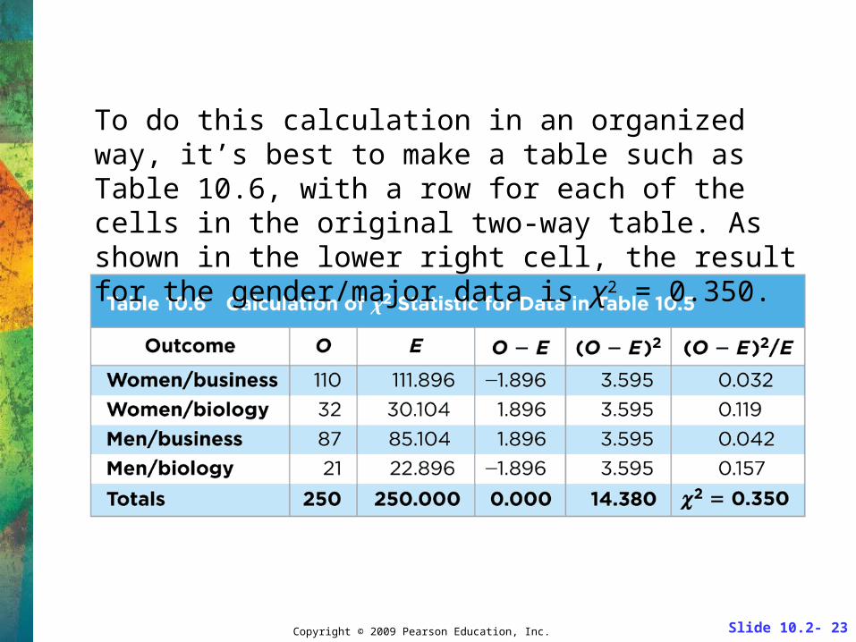
Finding the Chi-Square StatisticStep 1. For each cell in the two-way table, identify O as

the observed frequency and E as the expected frequency if the null hypothesis is true (no relationship between the variables).

Step 2. Compute the value (O - E)2/E for each cell.

Step 3. Sum the values from step 2 to get the chi-square statistic:

2 = sum of all values(O - E)2

E

The larger the value of 2, the greater the average difference between the observed and expected frequencies in the cells.

Slide 10.2- 23Copyright © 2009 Pearson Education, Inc.

To do this calculation in an organized way, it’s best to make a table such as Table 10.6, with a row for each of the cells in the original two-way table. As shown in the lower right cell, the result for the gender/major data is χ2 = 0.350.

Slide 10.2- 24Copyright © 2009 Pearson Education, Inc.

Finding the Frequencies Expected by Chance

Computing the Chi-Square Statistic

Making the Decision

Carrying Out the Hypothesis Test

The value of χ2 gives us a way of testing the null hypothesis of no relationship between the variables.

If χ2 is small, then the average difference between the observed and expected frequencies is small and we should not reject the null hypothesis.

If χ2 is large, then the average difference between the observed and expected frequencies is large and we have reason to reject the null hypothesis of independence.

Slide 10.2- 25Copyright © 2009 Pearson Education, Inc.

To quantify what we mean by “small” or “large,” we compare the χ2 value found for the sample data to critical values:

• If the calculated value of χ2 is less than the critical value, the differences between the observed and expected values are small and there is not enough evidence to reject the null hypothesis.

• If the calculated value of χ2 is greater than or equal to the critical value, then there is enough evidence in the sample to reject the null hypothesis (at the given level of significance).

Slide 10.2- 26Copyright © 2009 Pearson Education, Inc.

Table 10.7 gives the critical values of χ2 for two significance levels, 0.05 and 0.01. Notice that the critical values differ for different table sizes, so you must make sure you read the critical values for a data set from the appropriate table size row.

Slide 10.2- 27Copyright © 2009 Pearson Education, Inc.

For the gender/major data we have been studying in Tables 10.3 (slide 7) and 10.5 (slide 22), there are two rows and two columns (do not count the “total” rows or columns), which means a table size of 2 × 2.

Looking in the first row of Table 10.7 (previous slide), we see that the critical value of χ2 for significance at the 0.05 level is 3.841.

The chi-square value that we found for the gender/major data is χ2 = 0.350; because this is less than the critical value of 3.841, we cannot reject the null hypothesis.

Of course, failing to reject the null hypothesis does not prove that major and gender are independent. It simply means thatwe do not have enough evidence to justify rejecting the null hypothesis of independence.

Slide 10.2- 28Copyright © 2009 Pearson Education, Inc.

A (hypothetical) study seeks to determine whether vitamin C has an effect in preventing colds. Among a sample of 220 people, 105 randomly selected people took a vitamin C pill daily for a period of 10 weeks and the remaining 115 people took a placebo daily for 10 weeks. At the end of 10 weeks, the number of people who got colds was recorded. Table 10.8 summarizes the results. Determine whether there is a relationship between taking vitamin C and getting colds.

EXAMPLE 3 Vitamin C Test

Slide 10.2- 29Copyright © 2009 Pearson Education, Inc.

Solution: We begin by stating the null and alternative hypotheses.

H0 (null hypothesis): There is no relationship between taking vitamin C and getting colds; that is, vitamin C has no more effect on colds than the placebo.

Ha (alternative hypothesis): There is a relationship between taking vitamin C and getting colds; that is, the numbers of colds in the two groups are not what we would expect if vitamin C and the placebo were equally effective (or equally ineffective).

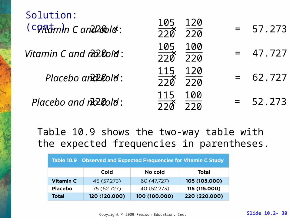
As always, we assume that the null hypothesis is true and calculate the expected frequency for each cell in the table. Noting that the sample size is 220 and proceeding as in Example 2, we find the following expected frequencies (next slide):

Slide 10.2- 30Copyright © 2009 Pearson Education, Inc.

105220220 × × = 57.273

120220Vitamin C and cold:

105220220 × × = 47.727

100220Vitamin C and no cold:

115220220 × × = 62.727

120220Placebo and cold:

115220220 × × = 52.273

100220Placebo and no cold:

Table 10.9 shows the two-way table with the expected frequencies in parentheses.

Solution: (cont.)

Slide 10.2- 31Copyright © 2009 Pearson Education, Inc.

We now compute the chi-square statistic for the sample data.

Table 10.10 shows how we organize the work; you should confirm all the calculations shown.

Solution: (cont.)

Slide 10.2- 32Copyright © 2009 Pearson Education, Inc.

To make the decision about whether to reject the null hypothesis, we compare the value of chi-square for the sample data, χ2 = 11.069, to the critical values from Table 10.7.

We look in the row for a table size of 2 × 2, because the original data in Table 10.8 have two rows and two columns (not counting the “total” values). We see that the critical value of χ2 for significance at the 0.01 level is 6.635.

Because our sample value of χ2 = 11.069 is greater than this critical value, we reject the null hypothesis and conclude that there is a relationship between vitamin C and colds.

That is, based on the data from this sample, there is reason to believe that vitamin C does have more effect on colds than a placebo.