Copyright © 2004 Brooks/Cole, a division of Thomson Learning, Inc. 1 Chapter 8 Network Models to accompany Operations Research: Applications & Algorithms,

Copyright © 2004 Brooks/Cole, a division of Thomson Learning, Inc.

1

Chapter 8Network Models

to accompanyOperations Research: Applications & Algorithms,

4th edition, by Wayne L. Winston


2

Description

Many important optimization problems can be analyzed by means of graphical or network representation. In this chapter the following network models will be discussed:

1. Shortest path problems

2. Maximum flow problems

3. CPM-PERT project scheduling models

4. Minimum Cost Network Flow Problems5. Minimum spanning tree problems


3

WHAT IS CPM/PERT FOR?

CPM/PERT are fundamental tools of project management and are used for one of a kind, often large and expensive, decisions such as building docks, airports and starting a new factory. Such decisions can be described via mathematical models, but this is not essential. Some would argue that CPM/PERT is not a pure OR topic. CPM/PERT really falls into gray area that can be claimed by fields other than OR also.


4

General Comments on CPM/PERT vs. ALB

Assembly Line Balancing (ALB) are naturally not discussed in this text, but it is important to be aware of the huge difference between the ALB and CPM/PERT concepts because the precedence diagrams look so similar.

Activity on node (AON) method of network precedence diagram drawing (not used in this chapter) and the ALB diagram are identical looking at first. The ALB deals with small repetitive items such as TV’s while CPM/PERT deals with large one of a kind projects.


5

8.1 Basic DefinitionsA graph or network is defined by two sets of symbols:• Nodes: A set of points or vertices(call it V) are called nodes of a graph or network.

• Arcs: An arc consists of an ordered pair of vertices and represents a possible direction of motion that may occur between vertices.

1 2

Nodes

1 2

Arc


6

• Chain: A sequence of arcs such that every arc has exactly one vertex in common with the previous arc is called a chain.

1 2

Common vertex between two arcs


7

• Path: A path is a chain in which the terminal node of each arc is identical to the initial node of next arc.

For example in the figure below (1,2)-(2,3)-(4,3) is a chain but not a path; (1,2)-(2,3)-(3,4) is a chain and a path, which represents a way to travel from node 1 to node 4.

2 3

1 4


8

8.2 Shortest Path Problems

Assume that each arc in the network has a length associated with it. Suppose we start with a particular node. The problem of finding the shortest path from node 1 to any other node in the network is called a shortest path problem. The general structure and solution methods of a shortest path problem will be shown in the following example.


9

Car (or machine) replacement example:

Let’s assume that we have just purchased a new car (or machine) for $12,000 at time 0. The cost of maintaining the car during a year depends on the age of the car at the beginning of the year, as given in the table below.

Age of Car (Years)

Annual Maintenance cost

Age of Car (Years)

Trade-in Price

0 $2,000 1 $7,000

1 $4,000 2 $6,000

2 $5,000 3 $2,000

3 $9,000 4 $1,000

4 $12,000 5 $0


10

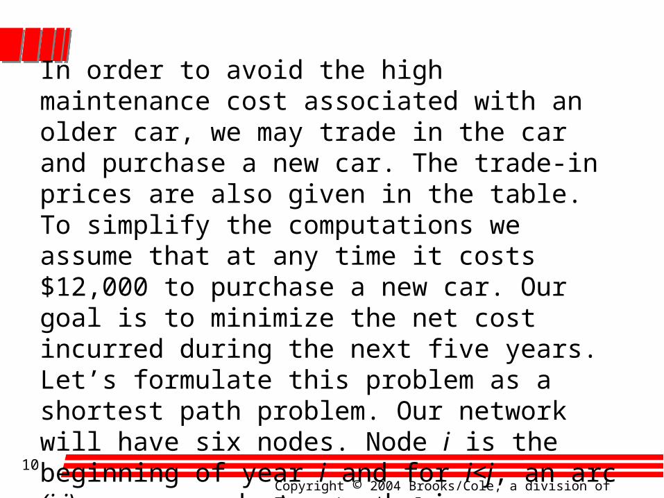
In order to avoid the high maintenance cost associated with an older car, we may trade in the car and purchase a new car. The trade-in prices are also given in the table. To simplify the computations we assume that at any time it costs $12,000 to purchase a new car. Our goal is to minimize the net cost incurred during the next five years. Let’s formulate this problem as a shortest path problem. Our network will have six nodes. Node i is the beginning of year i and for i<j, an arc (i,j) corresponds to purchasing a new car at the beginning of year i and keeping it until the beginning of year j. The length of arc (i,j) (call it cij) is the total net cost incurred from year i to j.


11

Thus:

cij = maintenance cost incurred during years i,i+1,…,j-1

+cost of purchasing a car at the beginning of year i

-trade-in value received at the beginning of year j.

Applying this formula to the information we will obtain the following:

c12=2+12-7=7 c13=2+4+12-6=12 c14=2+4+5+12-2=21

c15=2+4+5+9+12-1=31 c13=2+4+5+9+12+12-0=44 c23=2+12-7=7

c24=2+4+12-6=12 c25=2+4+5+12-2=21 c26=2+4+5+9+12-1=31

c34=2+12-7=7 c35=2+4+12-6=12 c36=2+4+5+12-2=21

c45=2+12-7=7 c46=2+4+12-6=12 c56=2+12-7=7


12

Network for minimizing car costs

1 654327 7 7 7 7

21

12

12

21

31

12

21

31

44

12

From the figure below we can see that both path 1-3-5-6 and1-2-4-6 will give us the shortest path with a value of 31.


13

8.3 Maximum Flow Problems

Many situations can be modeled by a network in which the arcs may be thought of as having a capacity that limits the quantity of a product that may be shipped through the arc. In these situations, it is often desired to transport the maximum amount of flow from a starting point (called the source) to a terminal point (called the sink). Such problems are called maximum flow problems.


14

An example for maximum flow problemSunco Oil wants to ship the maximum possible amount of oil (per hour) via pipeline from node so to node si as shown in the figure below.

so si21(2)2 (2)3 (2)2

(0)3

a0(2)

3(0)4 (0)1

The various arcs represent pipelines of different diameters. The maximum number of barrels of oil that can be pumped througheach arc is shown in the table above (also called arc capacity).

Arc Capacity

(so,1) 2

(so,2) 3

(1,2) 3

(1,3) 4

(3,si) 1

(2,si) 2


15

For reasons that will become clear soon, an artificial arc called a0 is added from the sink to the source. To formulate an LP about this problem first we should determine the decision variable.

Xij = Millions of barrels of oil per hour that will pass through arc(i,j) of pipeline.

For a flow to be feasible it needs to be in the following range:

0 <= flow through each arc <= arc capacity

And

Flow into node i = Flow out from node i


16

Let X0 be the flow through the artificial arc, the conservation of flow implies that X0 = total amount of oil entering the sink. Thus, Sunco’s goal is to maximize X0.

Max Z= X0

S.t. Xso,1<=2 (Arc Capacity constraints)

Xso,2<=3

X12<=3

X2,si<=2

X13<=4

X3,si<=1

X0=Xso,1+Xso,2 (Node so flow constraints)

Xso,1=X12+X13 (Node 1 flow constraints)

Xso,2+X12=X2,si (Node 2 flow constraints)

X13+X3,si (Node 3 flow constraints)

X3,si+X2,si=X0 (Node si flow constraints)

Xij>=0


17

One optimal solution to this LP is Z=3, Xso,1=2, X13=1, X12=1, Xso,2=1, X3,si=1, X2,si=2, Xo=3.


18

8.4 CPM and PERTNetwork models can be used as an aid in the scheduling of large complex projects that consist of many activities.

CPM: If the duration of each activity is known with certainty, the Critical Path Method (CPM) can be used to determine the length of time required to complete a project.

PERT: If the duration of activities is not known with certainty, the Program Evaluation and Review Technique (PERT) can be used to estimate the probability that the project will be completed by a given deadline.


19

CPM and PERT are used in many applications including the following:

• Scheduling construction projects such as office buildings, highways and swimming pools• Developing countdown and “hold” procedure for the launching of space crafts• Installing new computer systems• Designing and marketing new products• Completing corporate mergers• Building ships


20

To apply CPM and PERT, we need a list of activities that make up the project. The project is considered to be completed when all activities have been completed. For each activity there is a set of activities (called the predecessors of the activity) that must be completed before the activity begins. A project network is used to represent the precedence relationships between activities. In the following discussions the activities will be represented by arcs and the nodes will be used to represent completion of a set of activities (Activity on arc (AOA) type of network).

1 32A B

Activity A must be completed before activity B starts


21

While constructing an AOA type of project diagram one should use the following rules:• Node 1 represents the start of the project. An arc should lead from node 1 to represent each activity that has no predecessors.

• A node (called the finish node) representing the completion of the project should be included in the network.

• Number the nodes in the network so that the node representing the completion time of an activity always has a larger number than the node representing the beginning of an activity.

• An activity should not be represented by more than one arc in the network

• Two nodes can be connected by at most one arc.

To avoid violating rules 4 and 5, it can be sometimes necessary to utilize a dummy activity that takes zero time.


22

An example for CPM

Widgetco is about to introduce a new product. A list of activities and the precedence relationships are given in the table below. Draw a project diagram for this project.

Activity Predecessors Duration(days)

A:train workers - 6

B:purchase raw materials - 9

C:produce product 1 A, B 8

D:produce product 2 A, B 7

E:test product 2 D 10

F:assemble products 1&2 C, E 12


23

Project Diagram for Widgetco

1

65

42

3A 6

B 9

Dummy

C 8

D 7

E 10

F 12

Node 1 = starting nodeNode 6 = finish node


24

Important definitions for computation

Early Event Time: The early event time for node i, represented by ET(i), is the earliest time at which the event corresponding to node i can occur.

Late Event Time: The late event time for node i, represented by LT(i), is the latest time at which the event corresponding to node i can occur without delaying the completion of the project.


25

Computation of early event time

To find the early event time for each node in the project network we follow the steps below:• Find each prior event to node i that is connected by an arc to node i. These events are immediate predecessors of node i.• To the ET for each immediate predecessor of the node i add the duration of the activity connecting the immediate predecessor to node i.• ET(i) equals the maximum of the sums computed in previous step.


26

Computing ET(i). We start with the beginning node

3

4

5

6

8

4

3

ET(1)=0 (The starting node is always 0)

Let’s say ET(3)=6ET(4)=8, ET(5)=10

133)5(

124)4(

148)3(

max)6(

ET

ET

ET

ET

ET(6)=14


27

Computation of late event time

To compute LT(i) we begin with the finish node and go backwards and we follow the steps below:• Find each node that occurs after node i and is connected to node i by an arc. These events are immediate successors of node i.• From the LT for each immediate successor to node i subtract the duration of the activity joining the successor the node i.• LT(i) is the smallest of the differences determined in previous step.


28

Let’s compute LT(I)’s for the Widgetco example:

From the graph we know that the late completion time for node 6 is 38. Since node 6 is the only immediate successor of node 6, LT(5)=LT(6)-12=26. Same way LT(4)= LT(5)-10=16.

Nodes 4 and 5 are the immediate successors of node 3. Thus;

90-LT(3)LT(2)

188)5(

97)4(min)3(

LT

LTLT


29

36)3(

09)2(min)1(

LT

LTLT


30

Total Float

Before the project is begun, the duration of each activity is unknown, and the duration of each activity used to construct the project network is just an estimate of the activity’s actual completion time. The concept of total float of an activity can be used as a measure of how important it is to keep each activity’s duration from greatly exceeding our estimate of its completion time. Total float is represented by TF(i,j) and equals:

TF(i,j)=LT(j)-ET(i)-tij


31

For Widgetco example ET(i)’s and LT(i)’s are as follows:

Node ET(i) LT(i)

1 0 0

2 9 9

3 9 9

4 16 16

5 26 26

6 38 38


32

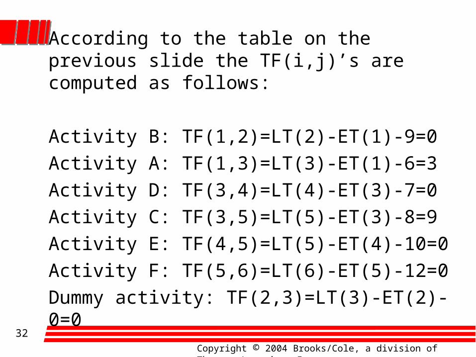
According to the table on the previous slide the TF(i,j)’s are computed as follows:

Activity B: TF(1,2)=LT(2)-ET(1)-9=0

Activity A: TF(1,3)=LT(3)-ET(1)-6=3

Activity D: TF(3,4)=LT(4)-ET(3)-7=0

Activity C: TF(3,5)=LT(5)-ET(3)-8=9

Activity E: TF(4,5)=LT(5)-ET(4)-10=0

Activity F: TF(5,6)=LT(6)-ET(5)-12=0

Dummy activity: TF(2,3)=LT(3)-ET(2)-0=0


33

Critical path

• An activity with a total float of zero is a critical activity• A path from node 1 to the finish node that consists entirely of critical activities is called a critical path.

For Widgetco example 1-2-3-4-5-6 is a critical path.


34

Free Float

Free float is the amount by which the starting time of the activity corresponding to arc(i,j) can be delayed without delaying the start of any later activity beyond the earliest possible starting time. Free float is calculated as follows:

FF(I,j)=ET(j)-ET(i)-tij


35

According to the table on the previous slide the FF(i,j)’s are computed as follows:

Activity B: FF(1,2)=9-0-9=0

Activity A: FF(1,3)=9-0-6=3

Activity D: FF(3,4)=16-9-7=0

Activity C: FF(3,5)=26-9-8=9

Activity E: FF(4,5)=26-16-10=0

Activity F: FF(5,6)=38-26-12=0

For example a delay up to 9 days in the start or duration of activity C will not delay the start of later activities.


36

Using LP to find a critical pathDecision variable:

Xij:the time that the event corresponding to node j occurs

Since our goal is to minimize the time required to complete the project, we use an objective function of:

Z=XF-X1

Note that for each activity (i,j), before j occurs , i must occur and activity (i,j) must be completed.


37

Min Z =X6-X1

S.T. X3>=X1+6 (Arc (1,3) constraint)

X2>=X1+9 (Arc (1,2) constraint)





X3>=X2 (Arc (2,3) constraint)

The optimal solution to this LP is Z=38, X1=0, X2=9, X3=9, X4=16, X5=26, X6=38


38

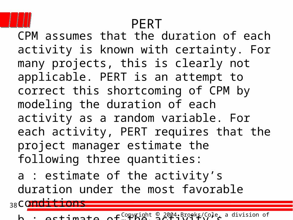
PERTCPM assumes that the duration of each activity is known with certainty. For many projects, this is clearly not applicable. PERT is an attempt to correct this shortcoming of CPM by modeling the duration of each activity as a random variable. For each activity, PERT requires that the project manager estimate the following three quantities:

a : estimate of the activity’s duration under the most favorable conditions

b : estimate of the activity’s duration under the least favorable conditions

m : most likely value for the activity’s duration


39

Let Tij be the duration of activity (i,j). PERT requires the assumption that Tij follows a beta distribution. According to this assumption, it can be shown that the mean and variance of Tij may be approximated by

36

)(var

6

4)(

2abT

bmaTE

ij

ij


40

PERT requires the assumption that the durations of all activities are independent. Thus,

pathji

ijTE),(

)(

pathji

ijT),(

var

: expected duration of activities on any path

: variance of duration of activities on any path


41

Let CP be the random variable denoting the total duration of the activities on a critical path found by CPM. PERT assumes that the critical path found by CPM contains enough activities to allow us to invoke the Central Limit Theorem and conclude that the following is normally distributed:

thcriticalpaji

ijTCP),(


42

a, b and m for activities in Widgetco

Activity a b m

(1,2) 5 13 9

(1,3) 2 10 6

(3,5) 3 13 8

(3,4) 1 13 7

(4,5) 8 12 10

(5,6) 9 15 12


43

According to the table on the previous slide:

136

)915(var,12

6

48159)(

44.036

)812(var,10

6

40128)(

436

)113(var,7

6

28131)(

78.236

)313(var,8

6

32133)(

78.136

)210(var,6

6

24102)(

78.136

)513(var,9

6

36135)(

2

5656

2

4545

2

3434

2

3535

2

1313

2

1212

TTE

TTE

TTE

TTE

TTE

TTE


44

Of course, the fact that arc (2,3) is a dummy arc yields

E(T23)=varT23=0

The critical path was 1-2-3-4-5-6. Thus,

E(CP)=9+0+7+10+12=38

varCP=1.78+0+4+0.44+1=7.22

Then the standard deviation for CP is (7.22)1/2=2.69

And

13.0)12.1()69.2

3835

69.2

38()35(

ZP

CPPCPP


45

PERT implies that there is a 13% chance that the project will be completed within 35 days.


46

8.5 Minimum Cost Network Flow Problems

The transportation, assignment, transshipment, shortest path, maximum flow, and CPM problems are all special cases of minimum cost network flow problems (MCNFP). Any MCNFP can be solved by a generalization of the transportation simplex called the network simplex.


47

To define MCNFP, let

Xij= number of units of flow sent from node i to node j through arc(i,j)

bi= net supply (outflow-inflow) at node i

cij= cost of transporting 1 unit of flow from node i to node j via arc(i,j)

Lij= lower bound of flow through arc(i,j) (if there is no lower bound, let Lij=0)

Uij= upper bound of flow through arc(i,j) (if there is no upper bound, let Uij=infinity)


48

Then the MCNFP can be modeled as follows:

ijijij

j k

ikiij

allarcs

ijij

UXL

bXXts

Xc

..

min

(for each node i in the network)

(for each arc in the network)


49

Formulating a transportation problem as an MCNFP

Consider the transportation problem below:

1

2 4

3

Supply point 1

Supply point 2 Demand point 2

Demand point 1

1 2 4 (Node 1)

3 4 5 (Node 2)

6 (Node 3) 3 (Node 4)


50

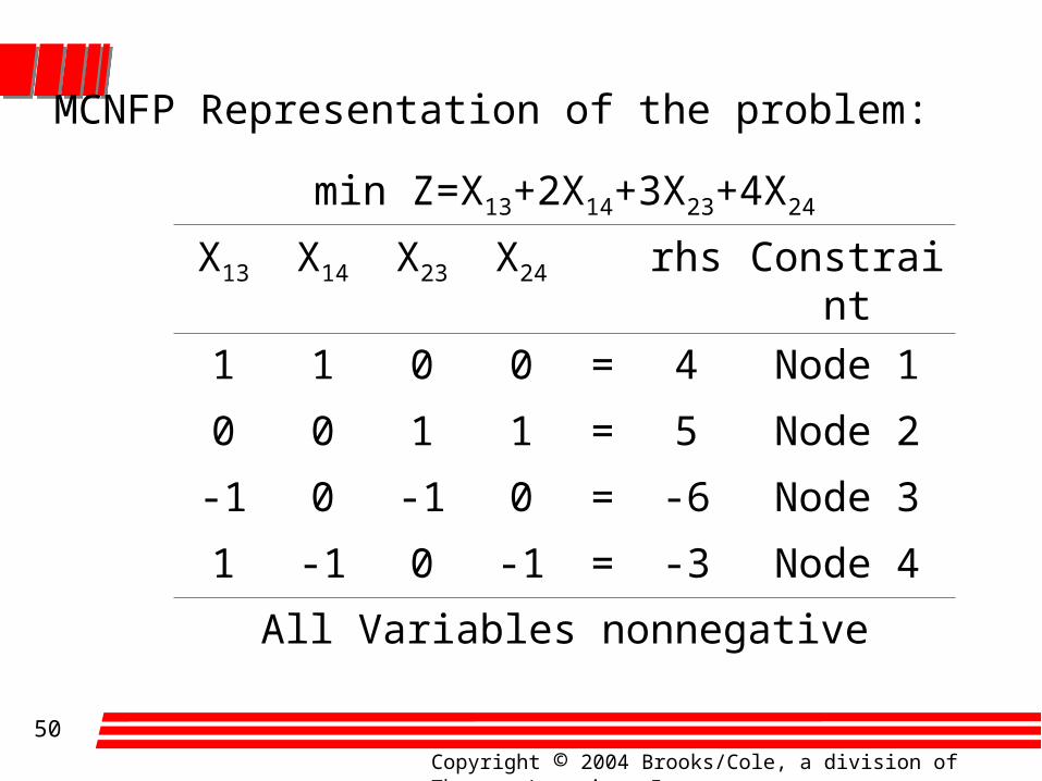
MCNFP Representation of the problem:

min Z=X13+2X14+3X23+4X24

X13 X14 X23 X24 rhs Constraint

1 1 0 0 = 4 Node 1

0 0 1 1 = 5 Node 2

-1 0 -1 0 = -6 Node 3

1 -1 0 -1 = -3 Node 4

All Variables nonnegative


51

8.6 Minimum Spanning Tree Problems

Suppose that each arc (i,j) in a network has a length associated with it and that arc (i,j) represents a way of connecting node i to node j. For example, if each node in a network represents a computer in a computer network, arc(i,j) might represent an underground cable that connects computer i to computer j. In many applications, we want to determine the set of arcs in a network that connect all nodes such that the sum of the length of the arcs is minimized. Clearly, such a group of arcs contain no loop.


52

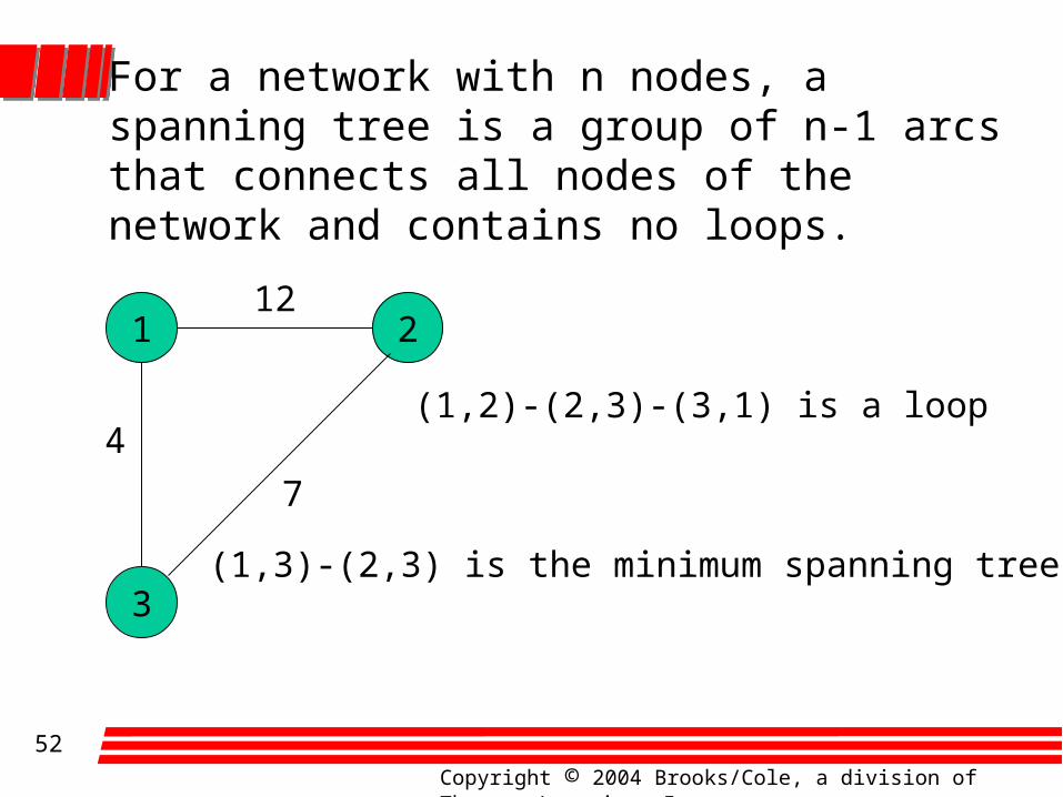
For a network with n nodes, a spanning tree is a group of n-1 arcs that connects all nodes of the network and contains no loops.

1

3

212

7

4(1,2)-(2,3)-(3,1) is a loop

(1,3)-(2,3) is the minimum spanning tree


53

The following method (MST Algorithm) may be used to find a minimum spanning tree:

• Begin at any node i, and join node i to the node in the network (call it node j) that is closest to node i. The two nodes i and j now form a connected set of nodes C={i,j}, and arc (i,j) will be in the minimum spanning tree. The remaining nodes in the network (call them Ć) are referred to as the unconnected set of nodes.


54

• Now choose a member of Ć (call it n) that is closest to some node in C. Let m represent the node in C that is closest to n. Then the arc(m,n) will be in the minimum spanning tree. Now update C and Ć. Since n is now connected to {i,j}, C now equals {i,j,n} and we must eliminate node n from Ć.

• Repeat this process until a minimum spanning tree is found. Ties for closest node and arc to be included in the minimum spanning tree may be broken arbitrarily.


55

Example: The State University campus has five computers. The distances between computers are given in the figure below. What is the minimum length of cable required to interconnect the computers? Note that if two computers are not connected this is because of underground rock formations.

4

2

5

3

1

6

4

5

1

3

2

2

2

4


56

Solution: We want to find the minimum spanning tree.• Iteration 1: Following the MST algorithm discussed before, we arbitrarily choose node 1 to begin. The closest node is node 2. Now C={1,2}, Ć={3,4,5}, and arc(1,2) will be in the minimum spanning tree.

4

2

5

3

1

6

4

5

1

3

2

2

2

4


57

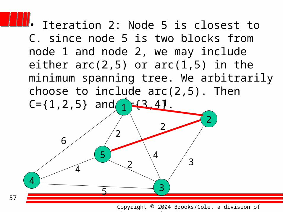
• Iteration 2: Node 5 is closest to C. since node 5 is two blocks from node 1 and node 2, we may include either arc(2,5) or arc(1,5) in the minimum spanning tree. We arbitrarily choose to include arc(2,5). Then C={1,2,5} and Ć={3,4}.

4

2

5

3

1

6

4

5

1

3

2

2

2

4


58

• Iteration 3: Since node 3 is two blocks from node 5, we may include arc(5,3) in the minimum spanning tree. Now C={1,2,5,3} and Ć={4}.

4

2

5

3

1

6

4

5

1

3

2

2

2

4


59

• Iteration 4: Node 5 is the closest node to node 4. Thus, we add arc(5,4) to the minimum spanning tree.

We now have a minimum spanning tree consisting of arcs(1,2), (2,5), (5,3), and (5,4). The length of the minimum spanning tree is 1+2+2+4=9 blocks.

4

2

5

3

1

6

4

5

1

3

2

2

2

4

Copyright © 2004 Brooks/Cole, a division of Thomson Learning, Inc. 1 Chapter 8 Network Models to accompany Operations Research: Applications & Algorithms,

Documents

division of thomson

arc slide

shortest path problems

following network models

network representation

winston slide

cpmpert deals

terminal node