Coping with Prosperity: The Response of Parents’ Child Care Time Use to Rising Earnings

1

Coping with Prosperity: The Response of Parents’ Child Care Time Use to

Rising Earnings

James M. Payne

Friday Afternoon Research GroupNovember 15, 2013

Coping with Prosperity: The Response of Parents’ Child Care Time Use to

Rising Earnings

2

Coping with Prosperity

• FACETIME—direct child care time• Physical & medical care• Reading, playing, sports, arts & crafts• Schooling & homework• Conversing

• BEHALFTIME—indirect child care time• Organizing and planning • Attending events, conferences, etc. • Dropping off/picking up/waiting • Obtaining medical care • Using child care services

Defining the dependent variables

Defining the dependent variables

3

• Parents seek to accumulate human capital in their children,with household production function:

human capital = f (FACETIME, Market services)

wheremarket services = f (Purchased services,

BEHALFTIME)

An increase in parents’ wage rates raises:• nominal incomes, and thus demand for human

capital in children• absolute prices of both own time and market

services, and the relative price of own time

Propositions Coping with Prosperity Propositions

4

• Expectation: Rising wages will lead to• an increase in FACETIME (probably)• an increase in market services

(unambiguously) and hence in BEHALFTIME• an increase in BEHALFTIME relative to

FACETIME

Propositions Coping with Prosperity Propositions

5

Wages child care time use is well established, but . . .

no studies have separated the income and price effects

Challenges (1) Coping with Prosperity Challenges

6

Zeroes in time use data A. 4 sources of zeroes

1. measurement error2. the individual will not participate in the activity3. corner solution4. diary window is shorter than the consumption period

B. Log transformation cannot be used to reduce heteroscedasticity

C. Tobit models common, but generate biased estimatesGould (1992), Keen (1986), Daunfeldt and Hellström (2007), Stewart (2009), Frazis and Stewart (2010)

Challenges (2) Coping with Prosperity Challenges

7

Wage variable problems

--endogeneity

--sample selection bias

Challenges (3) Coping with Prosperity Challenges

8

Missing income data in the Current Population Survey (CPS)

A. 34% missing wage data (2003) with negative selectionHeckman and LaFontaine (2006); 15.6% in my parents-only ATUS sample

B. Census’ modified hot deck imputation produces match biasHirsch and Macpherson (2004), Bollinger and Hirsch (2006, 2010)

Challenges (4) Coping with Prosperity Challenges

9

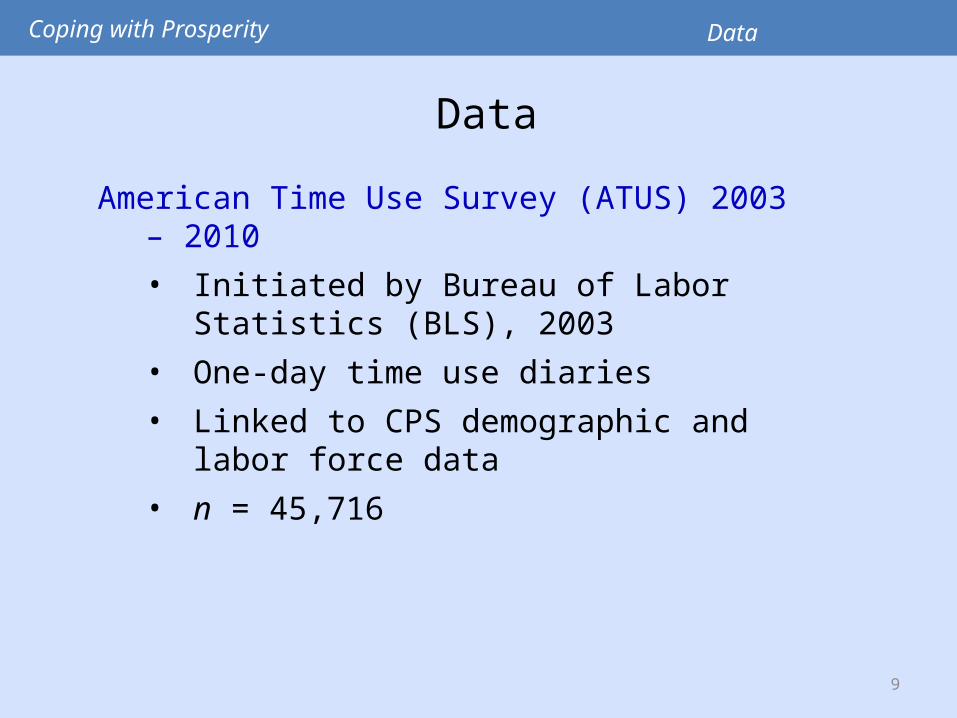
DataAmerican Time Use Survey (ATUS) 2003 –

2010• Initiated by Bureau of Labor Statistics

(BLS), 2003• One-day time use diaries• Linked to CPS demographic and labor

force data• n = 45,716

Coping with Prosperity Data

10

Coping with Prosperity

Descriptive statistics(minutes on diary day)

Two dependent variables

11

Coping with Prosperity

• Two inputs for producing human capital in children:

• Own time, which is FACETIME with price pf

• Market services (S)• Two components:• Purchases (P) with share γ and price pp • BEHALFTIME with share τ and price pb = pf • γ + τ = 1

Theoretical model

Theoretical model

12

Coping with Prosperity

Key point: How will a change in hourly earnings (w) affect input prices?

• pf : FACETIME consists only of time, so pf = w, = 1

• ps = γpp + τpb (weighted average of component prices)

• = 0 (prices of services are orthogonal to w)

• = τ (since pb = pf and = 1)

• So = τ < 1: an increase in earnings reduces the price of market services S relative to FACETIME, and . . .

• predicts that BEHALFTIME will be substituted for FACETIME

Theoretical model

13

Coping with Prosperity

Challenges (4): Estimating earnings from CPS • Use updated ATUS earnings data

• If available and valid, use hourly wage rate (TRERNHLY)

• If not, use weekly earnings (TRERNWA) divided by usual weekly work hours (TEHRUSLT)

• If topcoded, use estimates from Hirsch and Macpherson (2011)

• If not available, set to missing and impute later

• Adjust to 2003 constant dollars using CPI-U-SL to create rEARNHR

ATUS earnings data

14

Challenges (4): Multiple imputation (MI) of missing data• Rubin (1987)

• Process is intended to . . .• Fill blanks with “neutral” values• Preserve variation in the data

• Use EM/MCMC multiple imputation method

• Create several (m) different data sets, and• Model each set (imputation)

separately• Combine estimates using Rubin’s

Rule

Coping with Prosperity Multiple imputation

15

Coping with Prosperity

Multiple imputation

• Impute all missing covariates• Create m = 10 imputed data sets

Multiple imputation

16

Coping with Prosperity

Challenges (3): Endogeneity and sample selection in real hourly

earnings (rEARNHR)• Two problems—rEARNHR is:

• Endogenous with child care time (Heckman r = 0.14, p-value < 0.001)

• Unobserved for nonworking parents

ATUS earnings data

17

Coping with Prosperity

• Two-step solution—Millinet (2001) from Amemiya (1985):Heckman (1979) sample selection model, with

• 1st step: probit model—estimate probability of being employed (WORKING = 1)

• 2nd step: Include instrument (METRO) in OLS model for estimated real hourly earnings

• Result: one estimated earnings variable, rEARNHRhat, accommodating both endogeneity and sample selection bias

ATUS earnings data

18

Coping with Prosperity

1st step probit (Heckman) for WORKING = 1

2nd step OLS (Heckman) for rEARNHRhat

Instrument for

endogeneity

(METRO*)

double hurdle

models with x = rEARNHRhat

• Two-step solution

ATUS earnings data

19

Coping with Prosperity Inverse hyperbolic sine

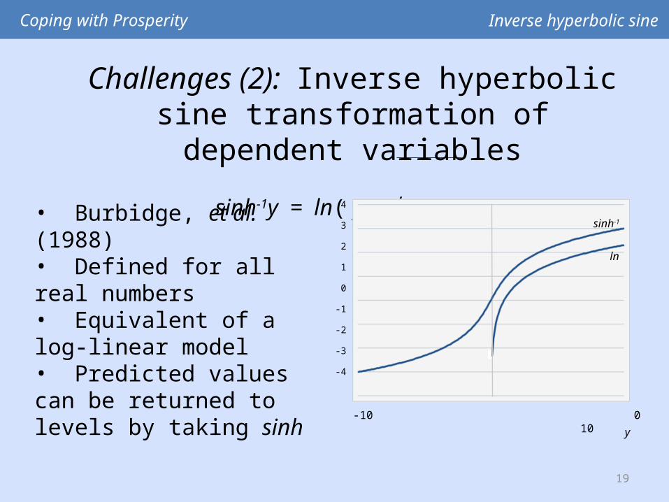
Challenges (2): Inverse hyperbolic sine transformation of dependent

variablessinh-1y = ln( y + √ y2 + 1 )• Burbidge, et al.

(1988)• Defined for all real numbers• Equivalent of a log-linear model• Predicted values can be returned to levels by taking sinh

4

3

2

1

0

-1

-2

-3

-4

-10 0 10 y

sinh-1

ln

20

Challenges (2): Double hurdle model

• Cragg (1971), Lin & Schmidt (1984)

• Assumes a corner solution

• Zero time use observations arise because some people never do the activity

• Two hurdles to engaging in the activity:• 1st hurdle: choosing whether to do

the activity• 2nd hurdle: choosing how much to do

the activity

Coping with Prosperity Double-hurdle model

21

Coping with Prosperity Estimation—Double hurdle

Estimation—Double hurdle Two-part model—estimate, separately for both FACETIME and BEHALFTIME

A. First-hurdle probit models for all observations

B. Second-hurdle truncated normal models using OLS for nonzero observations of FACETIME and BEHALFTIME

22

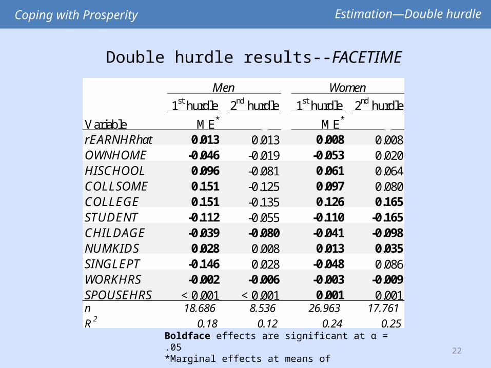
Coping with Prosperity Estimation—Double hurdle

Double hurdle results--FACETIME

Boldface effects are significant at α = .05*Marginal effects at means of regressors

1st hurdle 2nd hurdle 1st hurdle 2nd hurdleVariable ME* ME*

rEARNHRhat 0.013 0.013 0.008 0.008OWNHOME -0.046 -0.019 -0.053 0.020HISCHOOL 0.096 -0.081 0.061 0.064COLLSOME 0.151 -0.125 0.097 0.080COLLEGE 0.151 -0.135 0.126 0.165STUDENT -0.112 -0.055 -0.110 -0.165CHILDAGE -0.039 -0.080 -0.041 -0.098NUMKIDS 0.028 0.008 0.013 0.035SINGLEPT -0.146 0.028 -0.048 0.086WORKHRS -0.002 -0.006 -0.003 -0.009SPOUSEHRS < 0.001 < 0.001 0.001 0.001n 18,686 8,536 26,963 17,761 R 2 0.18 0.12 0.24 0.25

Men Women

23

Coping with Prosperity Estimation—Double hurdle

Double hurdle results--BEHALFTIME

Boldface effects are significant at α = .05*Marginal effects at means of regressors

1st hurdle 2nd hurdle 1st hurdle 2nd hurdleVariable ME* ME*

rEARNHRhat 0.003 0.012 0.008 -0.001OWNHOME -0.018 -0.020 -0.023 0.047HISCHOOL 0.042 0.171 0.022 0.163COLLSOME 0.061 0.231 0.041 0.172COLLEGE 0.071 0.123 0.037 0.334STUDENT -0.041 0.222 -0.025 -0.112CHILDAGE -0.002 -0.012 -0.005 -0.023NUMKIDS 0.038 0.078 0.053 0.106SINGLEPT 0.025 -0.406 0.044 0.170GOVEMP 0.042 -0.265 0.093 0.031PRIVEMP 0.021 -0.246 0.071 -0.089SELFEMP 0.051 -0.075 0.058 -0.092WORKHRS -0.001 -0.003 -0.001 -0.007SPOUSEHRS 0.001 -0.001 0.002 0.005n 18,686 3,731 26,963 9,570 R 2 0.07 0.08 0.10 0.12

Men Women

24

Coping with Prosperity

Challenges (1): Testing the hypothesis • Construct a ratio of BEHALFTIME and FACETIME and observe the effect of earnings on this

• Due to zeroes in the data, I construct the ratio of the marginal effects (ME) in the probit model

Theoretical model

25

Coping with Prosperity Substitution of BEHALFTIME for FACETIME

Substitution of BEHALFTIME for FACETIME

• 1st hurdle probit model—strong results for both variables for women• Fit a bivariate probit model for women for each imputed data set, and combine results using Rubin’s Rule• For both variables, calculate marginal effects at:• P10 Q1 Median Q3 P90 P95 of rEARNHRhat• P10 Q1 Median Q3 P90 of CHILDAGE• Medians of WORKHRS (30 hrs.) and SPOUSEHRS

(40 hrs.)• Means of other continuous variables• White, female, college graduate, US citizen,

married, homeowner, not a student, employed by a private firm, for a Monday in January, 2009

26

Coping with Prosperity Substitution of BEHALFTIME for FACETIME

Sensitivity analysis—marginal effects from bivariate probit model

*Earnings shown are the means of the 10 imputations; models were estimated using imputation-specific means

-0.0798 1.4760 -0.0029 1.5610 0.0853 1.6583 0.2181 1.8051 0.2977 1.8930 0.3742 1.9776

-0.0955 1.3589 -0.0185 1.4439 0.0696 1.5413 0.2024 1.6880 0.2820 1.7759 0.3586 1.8606

-0.1580 0.8907 -0.0811 0.9757 0.0071 1.0731 0.1399 1.2198 0.2195 1.3077 0.2960 1.3923

-0.2362 0.3054 -0.1592 0.3904 -0.0710 0.4878 0.0618 0.6346 0.1413 0.7225 0.2179 0.8071

-0.2831 -0.0457 -0.2061 0.0393 -0.1179 0.1367 0.0149 0.2834 0.0944 0.3713 0.1710 0.4559

Hourly earnings (2003$) (rEARNHRhat)*$2.69 $5.92 $9.61 $15.18 $18.55 $21.73

P 95

-0.0541 -0.0019 0.0514 0.1208 0.1572 0.1892

P 90P 10 Q 1 Median Q 3

0.2126

-0.0702 -0.0128 0.0452 0.1199 0.1588 0.1927

-0.1774 -0.0831 0.0066 0.1147 0.1679

0.3750

-0.7732 -0.4078 -0.1456 0.0973 0.1956 0.2700

† -5.2482 -0.8631 0.0524 0.2543

Age of youngest child

(CHILDAGE )

Q 3

P 90

P 100

2

6

11

15

Q 1

Median

MEBEHALFTIME /MEFACETIME

Cell contents: MEFACETIMEMEBEHALFTIME

27

Coping with Prosperity Substitution of BEHALFTIME for FACETIME

Comparisons from bivariate probit model

• Substitution of BEHALFTIME for FACETIME occurs as earnings rise• Effect is similar but: • smaller for blacks• smaller for high school graduates• larger for single parents

28

Coping with Prosperity Conclusions

Conclusions

Primary hypothesis • Parents substitute BEHALFTIME for FACETIME as earnings rise

Secondary hypotheses• Substitution effect is larger for single parents• For women, schooling positively affects the likelihood of engaging in both FACETIME and BEHALFTIME as well as the amount of time; for men, it affects the likelihoods only