COORDINATING STRATEGIC CAPACITY PLANNING IN THE ...sdw1/karabuk1.pdfindustry typically entails long-term strategic planning and short-term operational planning organized in a hierarchical

Technical Report 99T-11, Department of IMSE, Lehigh University

COORDINATING STRATEGIC CAPACITY PLANNING IN THE SEMICONDUCTOR INDUSTRY

SULEYMAN KARABUK and S. DAVID WU

Manufacturing Logistics Institute, Department of Industrial and Manufacturing Systems Engineering, Lehigh University, Bethlehem, Pennsylvania, [email protected]

Abstract

We study strategic capacity planning in the semiconductor industry. Working with a major US semiconductor manufacturer on the strategic configuration of their worldwide production capacities, we identify two unique characteristics of this problem as follows: (1) wafer demands and manufacturing capacity are both main sources of uncertainty, and (2) capacity planning must consider two distinct viewpoints: a product perspective concerning marketing and strategic demand management, and a process standpoint involving manufacturing, yield, and technology configuration. These two unique characteristics change, in a fundamental way, how strategic capacity planning problem should be approached. To describe this complex problem, we first formulate a multi-stage stochastic program with recourses where demand and capacity uncertainties are incorporated via a scenario structure. To reconcile the marketing and manufacturing perspectives to the problem, we consider a decomposition of the planning problem resembling decentralized decision-making involving the headquarter, the marketing manager, and the manufacturing manager. To study various trade-offs under this decentralized structure, we develop recourse approximation schemes simulating different decentralization strategies. These schemes vary in information requirements and complexity, while providing insight on the value of information in this environment. We conduct extensive experiments to analyze the characteristics of decisions under different levels of uncertainties, and assess the value of alternative schemes from the standpoint of computational requirements and solution quality. The results indicate that it is possible to arrive at near optimal solutions (within 6.5%) with information decentralization while using a fraction (less than 16.2%) of the computer time. Subject Classification: Facilities/equipment planning, capacity expansion: strategic capacity planning, Programming/stochastic: scenario analysis, recourse approximation, Production, planning: decentralized coordination.

2

Production capacity is the most significant portion of capital investment in semiconductor wafer manufacturing. Effective utilization and expansion of production capacity have significant cost implications, and arguably drives the profitability of the operation. Capacity management in the industry typically entails long-term strategic planning and short-term operational planning organized in a hierarchical manner. Strategic planning decisions include how much of which aggregate microelectronics technology to produce in what facilities, and which capacity element to expand within what timeframe so as to meet the projected demands. Operational planning determines capacity adjustment or reconfigurations among microelectronic technologies when more accurate demand and capacity information becomes available. Operational planning is frequent and dynamic so as to accommodate weekly production wafer "starts" to be released to manufacturing. In this paper we focus on the strategic capacity-planning problem while considering operational planning decisions as the short-term recourse of the capacity plan. Our study is based on real planning scenarios at a major US semiconductor manufacturer. One important characteristic of semiconductor capacity planning is that both product demands and manufacturing capacity are sources of uncertainty. As is the case in most hi-tech industries, the semiconductor market has a demand structure that is intrinsically volatile. A microelectronic chip that faces high demands today may be quickly outdated in a few months with the introduction of a next-generation chip requiring an enhanced manufacturing process. New manufacturing processes create high variability in the yields, and consequently uncertainty on the manufacturing throughput, which in turn lead to uncertainty in capacity estimation. Since the production volumes are typically high (for the interests of achieving economies of scale), extreme outcomes on demand and capacity realizations can lead to very undesirable business consequences. Therefore, it is important to consider different scenarios during long-term capacity planning. We propose a scenario based stochastic programming model to the problem, which produces a capacity configuration that hedges against extreme outcomes of demand and capacity fluctuation. 1. BACKGROUND 1.1 Context of the Semiconductor Industry

While capacity configuration and allocation are important decisions for any manufacturing company, a few factors make this problem especially crucial to the semiconductor industry. First is the high cost and long lead-time for equipment procurement and clean-room construction. The semiconductor wafer fabrication process requires state-of-the-art manufacturing equipment, many costs millions and must be ordered up to twelve months in advance. Wafers must be made in high purity clean rooms which cost anywhere from several hundred millions to a few billions to build and take one to two years to construct. Because of the long lead-time involved, capacity expansion decisions must be made far in advance. A wrong decision in either over- or under- estimation could have major impacts on profitability: suppose a decision is made to expand capacity for a certain technology but the demand does not materialize, significant loss could result due to under-utilization. On the other hand, if the capacity for a certain technology is not expanded timely to meet market demands, a significant loss of market share may result. Some believes that the semiconductor stock fluctuations in the earlier part of year 2000 are triggered by a combination of the above.

3

A second factor that exacerbates the impact of capacity planning in semiconductor is the rapid advancement of fab technologies and the pace of transition from old technologies to new. Semiconductor technologies can be defined in several ways, one of which is the space between features on a semiconductor die, known in the industry as line width. The most expensive and crucial pieces of equipment in the wafer fabrication line are used in the photolithography process, where the chip features are defined on a silicon wafer. With each advancement in photolithography technology, new and more expensive equipment must be purchased so that features with smaller line widths can be produced. Although the equipment is more expensive, it allows the manufacturer to either make smaller chips or fit more features on the same size chip, effectively reducing manufacturing costs for a given chip functionality. Another factor in the advancement of semiconductor manufacturing technology is the size of the wafers. Equipment manufacturers are continuously trying to increase the wafer size, which increases the number of chips to be made at once and produces higher yields, which in turn reduces the unit manufacturing cost. As semiconductor technologies advance, the company must be prepared to switch manufacturing capability to the newer technologies. These transitions take time and they must be anticipated correctly. A premature transition will lead to costly under utilization, or forcing manufacturing to use newer, more expensive equipment to manufacture older technologies that do not generate expected revenue. An overdue transition lead to missed market opportunities, which also lead to lower ROI for the capital investment.

A third factor unique to the semiconductor industry is that manufacturing capacity often

suffers high variability. The aggregate notion of manufacturing capacity used during strategic planning is in reality an approximation at best. Given a particular capacity configuration for each clean room, the manufacturing manager still has much flexibility in how that capacity is utilized, and his/her decision will determine what the “effective capacity” ultimately is. For instance, newer equipment can typically be used to manufacture older technologies, albeit at a lower cost efficiency. Further, the “effective capacity” to manufacture the same technology is different in each location, depending upon the technology mixture (capacity configuration), the wafer size made in that facility, skill level of the labor, and myriad other factors. This is further complicated by contractual requirements with the customer, which may dictate that certain products must be made in certain locations. Finally, if there is not enough capacity in the company owned facilities, outsourced foundry capacity can be bought for some technologies, at a higher cost. If wafers are made at a foundry, there may be contractual requirements that specify a minimum purchase. All of these factors come into play to make manufacturing capacity a significant source of uncertainty at the point of strategic planning. 1.2 Related Literature The idea of incorporating uncertainty in mathematical modeling goes back to the early work of Dantzig (1955). Although this modeling view represents real world problems more accurately, it is not attractive for practical applications until recently due to its high computational requirement. With the availability of inexpensive computing power and sophisticated solvers, stochastic programming models are increasingly popular. Numerous stochastic programming models have been suggested for strategic decision making such as capacity planning, medium term production planning, and power generation planning (Takriti et. al. (1996)). Bienstock and Saphiro (1988) model the strategic resource acquisition decisions as a stochastic program with

4

recourse. They apply the model at an electric utility to make fuel contract, and plant construction decisions under demand uncertainty. In another study, Eppen et al. (1989) model the strategic capacity-planning problem of a major automobile manufacturer. Decisions in the model include setting up or shutting down facilities for some of the product lines under consideration. The main source of uncertainty in their model is product demand over a medium term planning period. In a more recent study Berman et. al. (1994) apply a stochastic programming model to solve for the capacity expansion problem in service industry with uncertain demand. Their model determines the size, location, and timing of the expansions so as to maximize the total expected profit. Escudero et al. (1993), analyze different modeling approaches to the production and capacity-planning problem using stochastic programming. For the semiconductor manufacturer in our study, capacity planning is an aggregate planning problem to be considered at the beginning of the planning year. We propose a unique two-stage stochastic program where the stage-one decisions concern about capacity expansions and configurations to be made here-and-now, while the stage-two decisions consider operational decisions as recourses carried out by two distinct decision entities: product (or marketing) managers (PMs), and manufacturing managers (MMs). PMs and MMs take different recuperative actions under each particular scenario realization of demand and capacity. The literature that studies the effects of multiple decision entities and decentralized information is known as multidivisional decision-making. In a typical setting, authority is delegated to different divisions of the firm so as to ease the complexity of information gathering, processing, and hence decision-making. Burton and Obel (1984) discuss the rational behind decentralization and review issues in designing decentralization mechanisms in detail. In the earlier literature of decentralized planning, the most widely used approach is to model the overall decision problem as a deterministic linear program, identify the decision entities (divisions) and their subproblems then apply mathematical decomposition techniques to facilitate the information flow between the decision entities and the central coordinator (Christensen and Obel (1978), Burton and Obel (1980), (Burton and Obel, (1995))). These previous studies focused on linear and deterministic decision models taking advantage of well-studied decomposition principles. We are not aware of any work in the literature that studies the effect of decentralization in a stochastic decision making environment. As we will demonstrate in the paper, the fact that each decision entity considers a different set of scenarios in their local decision problem creates challenging issues. 2. PROBLEM FORMULATION AND SOLUTION APPROACH 2.1. The Strategic Capacity Planning Problem For the semiconductor manufacturer we studied, strategic capacity planning is considered at the beginning of each fiscal year, with a typical time horizon of five years. Capacity planning can be described as an iterative process between the following two main components: (1) capacity expansion, given projected product demands, identify the required manufacturing technologies and their capacity levels to be physically expanded or outsourced through the planning period, and (2) capacity configuration, determine which facility is to be configured with which technologies mix. The overall objective is to meet a revenue model based on strategic demand planning (which blends demand forecasting and proactive market development strategies). This objective can be viewed as meeting projected demands with minimized total costs. Capacity is

5

expressed in terms of wafer starts per week and capacity configuration is the number of wafer starts for each technology at each facility throughout the planning horizon. Physical capacity-expansion requires a lead-time up to two years and these decisions are implemented once determined at the beginning of the planning period, i.e., fixed before actual demand and capacity realize. Outsourcing arrangements need a shorter lead-time and can be delayed till uncertainty is somewhat reduced during the planning period. Capacity configuration decisions are subject to adjustments throughout the year in order to accommodate unforeseen changes in capacity and demand. The decisions involed in strategic capacity planning are as follows: xijt, the number of wafer starts per week for technology i (i∈M) to be configured at facility j (j∈F) during planning period t (t∈T), σjt and yjt represent 0-1 capacity expansion decision, and the volume of expansion (in wafer starts), respectively, at facility j during period t. zijt represents the technology certification decision, a 0-1 variable indicating whether technology i should be certified for production at facility j in period t. To simplify the notation, we use the set names interchangeable with the set cardinality. The capacity configuration (xijt) and capacity expansion (yjt) variables are both continuous and nonnegative, whereas the capacity expansion (σjt) and technology certification (zijt) decisions are binary. These decisions represent the semiconductor headquarters’ strategic plan for medium- to long-term capacity expansion and configuration. The plan is implemented on a rolling horizon basis in that a new five-year plan is generated at the beginning of each year. We define the two elements of uncertainty, demand and capacity, as scenario sets S1 and S2, respectively. Each element s1∈S1 (s2∈S2) identify a demand (capacity) vector with probability of occurrence of πs1 (πs2). A scenario for the capacity-planning problem is fully described by a pair of demand and capacity vectors from S1 and S2. Let S be the set of all scenarios obtained by all combinations of demand and capacity possibilities and πs1s2 ((s1,,s2)∈S) be the probability obtained by πs1πs2 (demand and capacity scenarios are defined exogenously and independently). Recall that capacity configuration decisions are subject to adjustments throughout the year to accommodate demand and capacity variations. Change in capacity configuration is modeled as recourse to the strategic planning decision during operation when the plan unfolds. We define a positive and a negative configuration change under scenario (s1,s2) ∈S as +

21sijt,s/ and −21, ssijt/ ,

respectively. While changing capacity configurations is unavoidable, it is costly because this disrupts the regular flow of manufacturing which results in increased inventory and manufacturing cycle times. Although it is desirable to satisfy all demand from in-house production, for a certain type of capacity shortfall, outsourcing could be more economical. Preferably outsourcing is considered together with the option of building ahead in-house while carrying inventory through periods. We denote outsourcing and inventory decisions under different scenarios by variables Omts1s2, and Imts1s2 respectively. Note that holding inventory is highly undesirable in the semiconductor industry due to the volatile nature of demands and the fact that the chance of scraping on-hand inventory is as high as 50%. Another factor that influences the capacity planning decisions is the bias each product manager (PM) has about the supply source. Due to the perceived quality level and delivery performance, some manufacturing facilities are strongly preferred over others. Interestingly, some of these preferences are imposed by the customers, who would go so far as paying a premium to ensure

6

the manufacturing origin of their products. This factor is capture in the model, where we measure the violation of PMs’ supply preferences by a variable Eijts1s2 and assume that there is a profit loss associated with preference violations (an additional cost in the model). On the manufacturing side, due to high capital costs, it is desirable to keep the facilities highly utilized. We measure the amount of capacity usage that is required by MMs’ to achieve a target utilization level by variable Ujts1s2. This penalizes capacity under-utilization and ensures that expansions are not considered before existing capacity is utilized. Let cx

ijt, cσ

jt, cyjt, c

zijt, c

Ujt, c

Iit, c

Oit, c

Eijt denote the unit costs associated with the variable in the

superscript (e.g. cxijt is the unit cost associated with xijt). Capacity expansion costs and technology

certification costs are adjusted to reflect the time value of money, however, to simplify notation we do not express this explicitly. We define c+

ijt, c−ijt as the unit costs for positive and negative

configuration changes, respectively. Having laid out all the variables and parameters we can now define the cost-minimizing objective function. The objective is to minimize total costs involved in meeting all projected demand, which consists of total capacity expansion and expected production, configuration deviation, capacity under-utilization, inventory carrying, outsourcing and preference violation costs. The objective function is expressed more formally as follows:

)1(

))()((

cos

),(,

)()(

)()(

,,)(

),(

21

21

2121

21

21

21

21

2121

21

21

2121

21

21

∑ ∑∑∑ ∑∑∑ ∑∑∑ ∑∑

∑ ∑∑∑∑ ∑∑∑∑∑∑∑∑

∈ ∈∈∈ ∈∈

∈ ∈∈∈ ∈∈

∈ ∈ ∈

−−++

∈

∈ ∈∈ ∈∈ ∈∈ ∈ ∈

++

++

−+++

+++

Tt Njissijt

Eijt

Sssss

Tt Misits

Oit

Sssss

Tt Mi

sitsIit

Sss

ss

Tt Fj

sjtsUjt

Sss

ss

Tt Fj Missijt

xijtijtssijt

xijtijt

Sssss

Nji Tt

ijtzij

Fj Tt

jtyjt

Fj Tt

jtjt

Fj Mi Tt

ijtxij

EcOc

IcUc

cccc

zcyccxc

ts) (total Minimize

ππ

ππ

δδπ

σσ

Let pjts1s2 denote the capacity of facility j in period t under scenario s1s2. We describe the capacity availability constraints as follows. The capacity that will be available through expansion is assumed to be known with certainty, and once a capacity expansion is made it is available in succeeding periods too. An intermediate variable '

21sfmtsX is defined in (3) so that the actual

configuration can be measured under each scenario.

)3()(,,,

)2()(,,

21'

211

'

212121

2121

SssTtMiFjxX

SssTtFjypX

sijtssijtsijtsijts

t

jsjtsMi

sijts

∈∈∈∈∀−+=

∈∈∈∀+≤

−+=∈

∑∑δδ

ττ

Capacity expansion at each period are constrained by the upper and lower bounds (ujt and l jt respectively). The upper bound is imposed due to physical limitations such as space availability for installing machines, and the lower bound reflects the fact that once a new machine is installed, capacity is increased by at least a fixed amount. The expansion constraints can be described as follows.

7

)5(,

)4(,

TtFjuy

TtFjly

jtjtjt

jtjtjt

∈∈∀≤

∈∈∀≥

σ

σ

A single facility cannot manufacture all microelectronic products (each require a different technology) offered by the firm. Although there is always room to improve profitability by installing new equipment or implementing new process that expand the capability of a facility. For a facility to qualify for producing a certain microelectronics technology, a rather costly quality certificate must be obtained from an independent audit. This typically involves the testing of initial batches of wafers satisfying specified yield and quality requirements. Constraint set (6) enforces this certification constraint, where B is a sufficiently big number.

)6(,),(1

TtNjizBxt

ijijt ∈∈∀≤ ∑=τ

τ

The total capacity is the maximum capacity available for a product mix. Due to technological restrictions imposed by bottleneck resources in the clean room, a given technology can only use up a part of the total capacity in any given period. Let gij be the fraction of capacity of facility j that is available for technology i. Constraint set (7) describes these technology-related capacity restrictions.

)7()(,,,)( 211

'2121

SssTtMiFjypgXt

jsjtsijsijts ∈∈∈∈∀+≤ ∑=τ

τ

As a managerial policy at the semiconductor headquater, 90% capacity utilization is considered as a target, which forms a capacity upper bound. This is due to the historic observation that when facilities operate beyond a certain utilization level, throughput drops significantly due to increased equipment failures and congestion in the system. Constraint set (8) imposes the utilization rule.

)8()(,,)(9.0 211

'212121

SssTtFjypUXt

jsjtssjtsMi

sijts ∈∈∈∀+≥+ ∑∑=∈ τ

τ

At the strategic capacity planning phase, the policy of the firm is to satisfy all demands under every scenario. The demands can be balanced by either inventory from previous periods or outsourcing at that period as described by (9), where dits1s2 represents the demand for technology i during period t under scenario s1s2.

)9()(,, 211'

2121212121SssTtMidOIIX sitssitssitsssit

Fj

sijts ∈∈∈∀=+−+ −∈∑

Let hij represent the fraction of total demand for technology i that is preferred to be supplied by facility j. Constraint set (10) specifies supply preferences of the PMs, where N is the set of facility-technology pairs for which certification decisions are considered.

8

)10()(,,),( 21'

212121 SssTtNjidhEX sitsijsijtssijts ∈∈∈∀≥+

The beginning and ending inventory is desired to be zero for planning purposes. Costraint set (11) implements this decision rule.

)11(,0,)(,0 2121TtSssMiI sits =∈∈∀=

Let (SP) denote the strategic capacity-planning model described by (1) - (11). While this model captures all important aspects of the problem from the viewpoint of the semiconductor headquarter, it is difficult to gather all demand and capacity related information from the local divisions. Another concern is that with realistic size problems it may be difficult to solve (SP) optimally. In the next section, we develop alternative stochastic programming models, which approximate (SP) via different scenario approximation schemes. 2.2. A Decentralized Planning Model We now consider a decentralized planning viewpoint where PMs and MMs consider their own local decisions while the headquarter consider only global aspect of the problem. This particular viewpoint more accurately captures the dynamics of the capacity planning process in industry reality, while mathematically it could be viewed as an approximation of the “ideal” optimization problem. Before starting our exposition, we first make the observation that the strategic capacity planning problem (SP) is a multistage stochastic program with block separable recourse (Louveaux, 1986). Therefore, it can be posed as a two-stage stochastic model as follows: (SP)

),,,(),(

SzyxQzcyccxcMinimize SP

Nji Ttijt

zij

Fj Ttjt

yjt

Fj Ttjtjt

Fj Mi Ttijt

xij ++++ ∑ ∑∑∑∑∑∑∑∑

∈ ∈∈ ∈∈ ∈∈ ∈ ∈

σσ

subject to (4)-(6) where QSP(x,y,z,S) is the recourse function defined by the second stage problem:

−

++

++

−++

=

∑ ∑∑∑ ∑∑∑ ∑∑∑ ∑∑

∑ ∑∑∑

∈ ∈∈∈ ∈∈

∈ ∈∈∈ ∈∈

∈ ∈ ∈

−−++

∈

)11()7(),3(),2(..

))()((

),,,(

),(,

)()(

)()(

,,)(

21

21

2121

21

21

21

21

2121

21

21

2121

21

21

ts

EcOc

IcUc

ccccminimize

SzyxQ

Tt Nji

ssijtEijt

Sss

ss

Tt Mi

sitsOit

Sss

ss

Tt Misits

Iit

Sssss

Tt Fjsjts

Uj

Sssss

Tt Fj Missijt

xijitssijt

xijit

Sssss

SP

ππ

ππ

δδπ

In this two-stage setting, the first stage problem makes up the capacity expansion decisions of the headquarter (at the strategic level) whereas the second stage recourse problem constitutes operational level adjustments made by the PMs and MMs once a demand and/or capacity scenario is observed. Also observe that the second stage problem is a combined manufacturing and marketing subproblems bundled by the capacity reconfiguration variables for each scenario (i.e. +

21sijt,s/ and −21, ssijt/ ). Although one may quickly observe that the second stage problem is

separable by scenarios, this is not the most sensible way to decompose the decisions due to the way information is organized at the firm. From the viewpoint of decentralized decision making where main decision entitities or the PMs and MMs keep control over their local information, it

9

is useful to take the following point of view: the recourse problem represent the manufacturing (marketing) subproblem with complete information about capacity (demands) senarios and certain information about the demands (capacity), charaterized by senario set SMM (SPM). When complete and symmetrical information is available to PMs and MMs, the two versions of the recourse problems become one (i.e., SMM= SPM=S and constraints (2),(3),(7)-(11)). When partial and/or asymmetric information is available from the other side, PMs (MMs) must approximate the capacity (demands) scenarios from the manufacturing (marketing) side (i.e., SMM⊂ S, SPM⊂ S, and SMM≠ SPM) while considering a subset of the constraints (e.g., its own local constraints). To analyze this particular model of decentralized planning, we introduce the following notation: define +)(

21MM

sijtsδ and −)(21

MMsijtsδ as the capacity reconfiguration decisions of the manufacturing

managers, and +)(21

PMsijtsδ and −)(

21PM

sijtsδ as the desired resource adjustment of the product (marketing)

managers. Using these new variables, and scenario sets SMM and SPM, we defined the manufacturing managers' problem (MMP) and the product managers' problem (PMP) as follows. (MMP)

∑ ∑∑∑ ∑∑∑∈ ∈∈∈ ∈ ∈

−−++

∈

+−++Tt Fj

sjtsUj

Sss

ss

Tt Fj Mi

MMsijts

xijit

MMsijts

xijit

Sss

ss Uccccc

:costs) operating (expected Minimize

21

21

212121

21

21

)(

)()(

)(

))()(( πδδπ

subject to

MMt

jsjtssjtsMj

sijts

MMt

jsjtsijsijts

MMMMsijts

MMsijtsijtsijts

MMt

jsjts

Mi

sijts

SssTtFjypUX

SssTtMiFjypgX

SssTtMiFjxX

SssTtFjypX

∈∈∈∀+≥+

∈∈∈∈∀+≤

∈∈∈∈∀−+=

∈∈∈∀+≤

∑∑

∑

∑∑

=∈

=

−+=∈

)(,,)(9.0

)(,,,)(

)(,,,

)(,,

211

'

211

'

21)()('

211

'

212121

2121

212121

2121

ττ

ττ

ττ

δδ

(PMP)

∑ ∑∑∑ ∑∑∑ ∑∑∑ ∑∑∑

∈ ∈∈∈ ∈∈

∈ ∈∈∈ ∈ ∈

−−++

∈

++

+−++

Tt Nji

sijtsEijt

Sss

ss

Tt Mi

sitsOit

Sss

ss

Tt Misits

Iit

Sssss

Tt Fj Mi

PMsijts

xijit

PMsijts

xijit

Sssss

EcOc

Iccccc

:costs) fill order (expected Minimize

),()()(

)(

)()(

)(

21

21

2121

21

21

21

21

212121

21

21))()((

ππ

πδδπ

subject to

TtSssMiI

SssTtNjidhEX

SssTtMiFjxX

SssTtMidOIIX

PMsits

PMsitsijsijtssijts

PMPMsijts

PMsijtsijtsijts

PMsitssitsssitssti

Fj

sijts

,0,)(,0

)(,,),(

)(,,,

)(,,

21

21'

21)()('

21,,1,'

21

212121

212121

2121212121

=∈∈∀=

∈∈∈∀≥+

∈∈∈∈∀−+=

∈∈∈∀=+−+

−+

−∈∑

δδ

If we are to allow local decision makers to solve their own decision problems (MMP) and (PMP) instead of the bundled recourse problem QSP(x,y,z,S), a significant reduction of computational

10

requirement could be expected, as the cardinality of the scenario set may be significantly smaller (i.e., in the extreme case when MM and PM only consider their own scenarios, |S|=|SMM|× |SPM|). However, it is not difficult to see that doing so is equivalent to relaxing the following necessary bundling constraints between the two divisional subproblems when considered under QSP(x,y,z,S):

)13()(,,,

)12()(,,,

21)()(

21)()(

212121

212121

SssTtFjMi

SssTtFjMi

PMsijts

MMsijtssijts

PMsijts

MMsijtssijts

∈∈∈∈∀==

∈∈∈∈∀==−−−

+++

δδδ

δδδ

Solving (MMP) and (PMP) without constraints (12) and (13) will most likely lead to poor lower bound solution to QSP(x,y,z,S), thus the overall problem (SP). This should be intuitive because each subproblem misses very decisive information about the other side (i.e., demand or capacity), it is likely to generate highly biased decisions to its own favor, which in turn may steer the headquarter's solution away from the overall optimum. Specifically, the manufacturing subproblem (MMP) has no information about demand scenarios and how thir reconfiguration decisions may affect the costs of the marketing division. On the other hand, the marketing subproblem (PMP) uses only the configuration deviation costs to adjust local decisions of “how much supply to request” but without any information on capacity availability and utilization costs. The two sides are unlikely to reach any agreement, even less efficient coordination. From a pure computational point of view, traditional mathematical programming technique such as Lagrangean decomposition would suggest relaxing the bundling constraints while adding a Largrangean term in the subproblem objectives. Unfortunatly, this approach requires excessive communication between the two decision entities (on their recourse variable values, δPM and δMM). We propose a new form of decomposition motivated by the information requirements of this decentralized decision problem. The basic idea is that we require the MMs (PMs) to consider a version of the PMs’ (MMs’) problem as a second stage recourse problem of its own local decision problem, i.e., we reformulate each subproblem as a two-stage stochastic program with recourse where the first stage is the local decision problem MMP (PMP) while the recourse problem is defined as a model of it's opponent's subproblem PMP (MMP). The intuition behind this approach is that each decision maker contemplates a “model of others” when making its decisions since the other decision entities represent a main source of uncertainty to its decision problem. With this decomposition scheme, we compansate for the loss of information by relaxation of constraints (12) and (13). We expressed the reformulation as subproblems (MMP)' and (PMP)' as follows: (MMP) '

Minimize (MMP) + ),( )()(

2121

−+ MMsijts

MMsijts

MMQ δδ

where QMM(.)={ (PMP)| +)(21

MMsijtsδ → +)(

21PM

sijtsδ , −)(21

MMsijtsδ → −)(

21PM

sijtsδ }

(PMP)'

Minimize (PMP) + ),( )()(

2121

−+ PMsijts

PMsijts

PMQ δδ

where QPM(.)={ (MMP)| +)(21

PMsijtsδ → +)(

21MM

sijtsδ , −)(21

PMsijtsδ → −)(

21MM

sijtsδ }

11

The recourse functions QMM(.) and QPM(.) correspond to the manufacturing and marketing subproblems, respectively. Notice that both (MMP)' and (PMP)' are approximations for the term QSP(x,y,z,S), which is the recourse based on complete information in problem (SP). To establish a basis that would allow us to compare centralized vs. decentralized planning strategies, we now define decentralized planning as an approximation to the centralized planning problem (SP) as follows using (MMP)' and (PMP)'. (ASP)

''

),(

))(1()( PMPMMP

zcyccxcMinimizeNji Tt

ijtzij

Fj Tt

jtyjt

Fj Tt

jtjt

Fj Mi Tt

ijtxij

αα

σσ

−++

+++ ∑ ∑∑∑∑∑∑∑∑∈ ∈∈ ∈∈ ∈∈ ∈ ∈

subject to (4)-(6) and ]1,0[∈α . Problem (ASP) consists of stage 1 of problem (SP) plus a convex combination of two recourse approximations as described by (MMP)' and (PMP)'. The weight α can be interpreted as the headquarter’s way to reconcile operational decisions made by the divisions based on the perceived accuracy and information value of the related division’s computations. Throughout this study, we set α to 0.5. It should be clear that problem (ASP) approximates (SP) while at the same time attaining a structure suitable for decentralized planning. Interestingly, (ASP) takes the viewpoint that the headquarter makes stage-1 capacity expansion and configuration decisions considering future recourses to be made by manufacturing and marketing. Different from a typical two-stage stochastic program is the fact that decision makers who actually carry out the recourses are different from ones who make the first stage decision. This is in fact the very nature of the semiconductor capacity planning problem in reality. In other words, we assume that the recourse policy used under a particular scenario is not known exactly a priori and must be approximated at time zero. Coordination of the three decision entities: the headquarter, the PMs and the MMs ultimately drives the efficiency of the decision. This strategic decision structure suggests an operational structure for capacity adjustment over the course of the year where the recourse problems (MMP)' and (PMP)' represent base decision models for the local decision makers in manufacturing and marketing, respectively. 2.3 Solution Strategies for (ASP) and Their Implications on Information Usage We now define a few solution strategies for (ASP) so as to gain insights on the performance-computation trade-off when different forms of information are used. Full Recourse and No Recourse: Recall that the recourse function in subproblems (MMP)' and (PMP)' represent a "model of others" in the sense that it captures some aspects of the scenarios and constraints of the other side. Conceptually, the recourse term in the subproblems (MMP)' and (PMP)' can vary from a full description of the scenario of the other side (complete information, no approximation), to a complete empty set (no information). We refer to the former case as the full recourse model which corresponds to the original problem (SP) (i.e. (ASP) = (SP)), or the centralized model. We refer to the latter extreme as the no recourse model.

12

Partial Recourse: Since problems (MMP)' and (PMP)' are both posed as two-stage stochastic programs, we can apply recourse approximation methods to construct recourse functions for subproblems (i.e. QMM(.) and QPM(.)). One approach is to include all the constraints and decision variables but approximate the scenarios of the other side. Since the capacity and demand distributions are considered private information for the manufacturing and marketing divisions, respectively, this approximation is consistent with the information availability in real problems. Two most basic recourse approximation methods in the stochastic programming literature are Jensen's lower bound and Edmunsen-Madansky upper bound (Kall and Wallace (1994), and Birge and Louveaux (1996)) approximations for minimization problems. Jensen's lower bound is computed by using the expected value of random parameters in the recourse function. Modified this way the recourse function intentionally underestimates the true value over all values of the first stage variables. On the other hand, Edmunsen-Madansky upper bound is computed using an approximate distribution for the random parameters in the recourse. This distribution is constructed by taking the support points of the random variable distribution and resample the probability density function on these points. Edmunsen and Madansky prove that the recourse function formed this way provides an upper bound to the original over all values of first stage variables. Although simple and use little information about the random variables, the two methods are known to perform well in terms of approximating the original recourse function. We term this approximation as the partial recourse model. It is closer to the full recourse model in terms of information requirements and the degree of coupling between subproblems. There are several more sophisticated and accurate recourse approximation techniques in the literature (c.f., Birge and Wets (1986)), however, they also require a much increased information transparency to the headquater, which render them unsuitable for our study. Simple Recourse: The decisions that affect both subproblems are the capacity configuration decisions that are set by the headquarter (the stage 1 decision in (SP)). The two subproblems must compute their local costs as a function of the configuration decisions. Since both subproblems are expressed as linear programs, their corresponding recourse functions (in SP) are piecewise linear. We can therefore construct a linear approximation of this cost function as follows: first, include in the subproblem a deviation cost incurred to the other side for each unit of capacity configuration that deviates from some base configuration value. Define X*(MM) and X*(PM) as follows.

X*(MM) = {X(MM) | min (MMP)} X*(PM) = {X(PM) | min (PMP) s.t. +)(

21PM

sijtsδ = −)(21

PMsijtsδ = 0}

X*(MM) is the capacity configuration vector that optimizes the manufacturing subproblem. Similarly, X*(PM) minimizes the marketing subproblem which does not consider the capacity configuration deviations. Next, we make the following definitions.

C*(MM) = min (MMP) s.t. X= X*(MM) C*(PM) = min (PMP) s.t. +)(

21PM

sijtsδ = −)(21

PMsijtsδ = 0, X= X*(PM)

Consider the manufacturing subproblem (i.e. (MMP)) and the modified marketing subproblem (i.e. (PMP) s.t. +)(

21PM

sijtsδ = −)(21

PMsijtsδ = 0). If we set X=X* in both problems and solve them, the dual

13

variable values provide us with the unit cost of deviating from the configuration given by X* . In this setting, deviating from X* is the same as perturbing the right hand side of the relevant subproblem constraints. Let β∗(MM) (β∗(PM)) be the dual prices associated with unit deviations

(both positive and negative) in X*(MM) (X*(PM)), and −+ )()(

,MM*MM* δδ (

−+ )()(,

PM*PM* δδ ) be the

variables which measure the deviations from the capacity configuration that is optimized for the manufacturing (marketing) subproblem. Thus, we can define QMM(.) and QPM(.) for simple recourse as follows.

QMM(.)=min )*()*()*()*( )(11

11

1

PM

Tt Fj Mi

PMijts

PMijts

PMijt

Sss CX ++∑ ∑∑∑

∈ ∈ ∈

−+

∈

δβπ

s.t.

11)()*()*()( ,,,

111SsTtMiFjXX PM

ijtsPM

ijtsPM

ijtMM

ijts ∈∈∈∈∀−+= −+ δδ , and

QPM(.) = min )*()*()*()*( )(22

22

2

MM

Tt Fj Mi

MMijts

MMijts

MMijt

Sss CX ++∑ ∑∑∑

∈ ∈ ∈

−+

∈

δβπ

s.t.

22)()*()*()( ,,,

222SsTtMiFjXX MM

ijtsMM

ijtsMM

ijtPM

ijts ∈∈∈∈∀−+= −+ δδ

Note that the constant terms C*(MM) and C*(PM) are shown in the formulation for illustrative purposes. They do not go into the model during optimization. The above procedure is analogous to generating two cuts (around the optimal solution) in Benders' decomposition given the capacity configuration values that optimize each subproblem. From a different perspective, we can say that the “other side’s” subproblem is approximated by using a dual basis. Since the formulation of (MMP)' ((PMP)') with the above QMM(.) (QPM(.)) definition corresponds to a two-stage stochastic programming model with simple recourse (Kall and Wallace (1994)), we refer to this approach as the simple recourse model. The simple recourse model is in between partial recourse and no recourse models in terms of approximation complexity and information decentralization. In our analysis using the dual prices to determine configuration deviation costs (i.e. β∗(MM), β∗(PM)), we realized that the solution is quiet sensitive at X* in both subproblems. That is, for most unit deviations the basis changes, thus invalidates the dual prices. Since the simple recourse model is an approximation in itself, we wanted to obtain the deviation costs accurately in order not to cause more deterioration in the approximation. This requires solving the subproblem optimally for each unit deviation from X* and recording the objective function difference between the computed one and C*. Considering that we are changing the right hand side of a subproblem by one unit it takes only a few more iterations from the basis obtained for computing the X* , to find the new optimum. Hence, the computational burden that this approach brings over using the dual prices is negligible, but the accuracy it brings is significant. In this section we have developed four decentralized planning schemes that approximate the centralized model. In these approximation schemes, as the modeling complexity decreases, the degree of coupling between manufacturing and marketing subproblems also decreases. In the next section, we conduct intensive computational testing on these approximation schemes. We are particularly interested in the tradeoff between solution quality and the degree of “coupling”

14

between subproblems; we use this study as a means to analyze the cost-tradeoff between centralization and decentralization capacity planning. Further Discussions There are different decomposition techniques available to solve the stochastic models developed in this section (see Ruszczynski (1997)), among which Benders' decomposition (Benders (1962)) is the most widely used one due to its simplicity and effectiveness. Application of Benders' decomposition to solve the models in a decentralized environment can be interpreted as follows. The center announces a capacity configuration and expansion decision vector. The manufacturing and marketing subproblems solve (MMP)' and (PMP)' respectively and send their bid prices against the announced decisions. In return, the Headquarter takes a convex combination (as in the objective function of (ASP)) of the prices they receive from the subproblems to form an estimation of the cost function associated with their decisions (that is, add an optimality cut to the master problem). This is a typical resource-directive decomposition application, which will converge to the optimal solution of problem (ASP) at the end of iterations. For computational testing, we will solve each of the above approximation as modified versions of the monolithic model as opposed to implementing the actual decomposition algorithm one-by-one. In this way, we can isolate the merit of the proposed approximation methods without the bias introduced by any particular implementation. 3. COMPUTATIONAL EXPERIMENTS 3.1. Data generation To test a wide range of demand and capacity scenarios we use characteristics extracted from the semiconductor facility to generate experimental data. The data characteristics are consistent with that used by the planning specialist during annual capacity planning. To simulate matured technologies with stable demand, and new technologies with highly variable demand over time we generate the demands for a technology over multiple periods from a uniform distribution with mean and range drawn from two uniform distributions. The capacities from fab facilities are drawn from a uniform distribution whose mean is set equal to the total demand for that facility with the upper and lower supports set at 30% above and below of the mean, respectively. Negative values are truncated to zero. On average, taken over the instances used in the experiment, the total demand exceeds total capacity by about 10%. For each facility (technology), scenarios are generated by discretizing a normal distribution defined by the capacity (demand). The normal distribution is truncated at 3 times the standard deviation from the mean on both ends and divided into 6 equal intervals. The midpoints of the intervals are taken as the scenario values and the probability density contained in an interval is taken as the probability associated with that scenario. All capacity (demand) scenarios are applied to all facilities (products). Table 1 summarizes the parameters that have a common generation method over all the problem instances.

15

Table 1. Distributions used to generate common cost parameters Parameter Value distribution Parameter Value distribution pjt

A= F

dm

mt∑

pjt ~U(a*0.7,a*1.3)

dit a~U(300,600) b~U(50,150) dit~U(a-b/2, a+b/2)

ujt U(pjt* 0.30, pjt* 0.50) l jt U(pjt* 0.10, pjt* 0.15) hij U(dit*0.40, dit*0.80 ) gij U(pjt* 0.30, pjt* 0.70) cx

ij U (50,100) cEij U(100,200) cy

jt U(25,50) cUit 50 3.2. Experimental Design We identify three important factors that can affect the performance of the decision models: (i) degree of variability in both capacity and demand scenarios, (ii) the problem size, and (iii) the cost structure. Since all models use scenario approximation in the (second stage) recourse problem, as the variability in the scenario distribution increases the approximation error may also increase. In the experiment, we used coefficient of variation values of 0.1 and 0.3 to represent low and high variability, respectively. The simple recourse model approximates the decision variables and the constraints of the other side’s subproblem, hence, as the problem size increases the approximation quality may be affected. We therefore examine two levels of problem sizes. For small problems we set the number of facilities to 3, the number of technologies to 12 and the number of planning periods to 3 with 6 demand scenarios and 6 capacity scenarios defined per period. In addition, we set the cardinality of set N (technology facility pairs for which certification decisions are to be made) to 40% of the number of technologies and the set is formed by selecting random facility-technology pairs. We implemented all models in AMPL and used the CPLEX 6.5 solver. The problems are solved on a Pentium Celeron based PC running at 433 MHz with 128MB of memory. The resulting (SP) model has 21 binary, 15,129 variables with 10,602 linear constraints and on the average it takes 30 CPU seconds to find the optimal solution. For large problems, we increased the number of technologies from 12 to 18 and the number of planning periods from 3 to 5. The resulting problem has 50 binary, 37,725 variables with 26,310 linear constraints, which on the average takes 160 CPU seconds to find the optimal solution. Since there are many cost parameters involved in the model, we considered cost structure an additional experimental factor. Through initial trials, we identify a subset of cost factors that are most influential on the solution quality as follows: capacity expansion fixed cost, technology certification fixed cost, outsourcing cost, inventory carrying cost, and configuration deviation costs. We group these cost factors into two: (1) capacity expansion fixed costs and certification costs which affect the stage 1 costs and capacity expansion amount, and (2) outsourcing, inventory carrying and configuration deviation costs which effect whether the optimum solution will rely more on in-house capacity (including capacity expansions) or more on outsourcing. We consider two levels (high and low) for each parameter group which in turn defines four different cost structures (CS1-CS4) as summarized in Table 2. Given historic data we have in the semiconductor facility under study, we performed pilot experiments to set the distribution parameters such that under low expansion cost the total capacity expansions made is

16

approximately 8% of the total expected capacity (over all facilities and periods), whereas for high expansion cost this is reduces to 5%. Similarly, the low and high levels of outsourcing costs is set by pilot experiments as follows: we measured the ratio of total expected in-house production and total expected demand; at the low level, where outsourcing is relatively cheaper than inventory carrying and deviation costs, the ratio is set at 80%, whereas it is set at 95% at the high level where outsourcing is relatively more expensive. These conditions are consistent with the insights we have gained from experienced planners. Table 3 further summarizes the experimental factors and their levels. Table 2. Levels of the cost structure factor and their descriptions CS1 CS2 CS3 CS4 Expansion Cost Low Low High High Outsourcing Cost High Low High Low cS

jt U(30000,40000) U(30000,40000) U(70000,80000) U(70000,80000) cz

ij U(30000,40000) U(30000,40000) U(70000,80000) U(70000,80000) cO

it U(400,500) U(200,300) U(400,500) U(200,300) cI

it U(200,300) U(400,500) U(200,300) U(400,500) c+

it, c−it U(200,300) U(400,500) U(200,300) U(400,500)

Table 3. Experimental factors and their levels Experimental Factor Levels 1. Variability in capacity scenarios

(coefficient of variation) - Cap_CV 0.1 0.3

2. Variability in demand scenarios (coefficient of variation) - Dem_CV

0.1 0.3

3. Problem size (S=small, L=large) S L 4. Cost Structure CS1 - CS4 As discussed earlier, the strategic capacity planning decisions include capacity configuration, capacity expansion and certification, which make up the stage 1 of the (SP) model. The operational decisions correspond to stage 2 recourses and is computed only to determine the optimum stage 1 decisions rather than actual implementation. We therefore evaluate the four alternative recourse models (solution strategies for ASP) as follows: we first solve problem (ASP) using one of the three strategies (i.e. partial recourse (PR), simple recourse (SR), no recourse (NR), and full recourse (OPT)), then set the stage 1 decisions variables in (SP) to the solution obtained in (ASP), we then resolve (SP) optimally. The resulting solution is the simulated stochastic solution for problem (ASP), which we consider in the evaluations. We do not consider the CPU time used for finding the simulated solution value in the time comparison. Neither do we include the preprocessing time (i.e., CPU time involved to find the base configuration values and deviation cost coefficients) needed for the simple recourse approach. A common approach used to measure the benefits of stochastic analysis versus a deterministic one is to compute the Value of Stochastic Solution (VSS) (Birge and Louveaux, 1997). Since all the models developed in this study are different forms of Stochastic Programming models, we included the simulated stochastic solution of the deterministic model, which we denote by EEV, in the comparisons as an absolute performance minimum that any stochastic model must achieve.

17

We applied performance analysis on the proposed models using two main criteria: percent deviation from the overall stochastic optimal and computation time. We present the experimental results in the next section. 3.3. Experimental Results We identified two recourse approximation methods that can be used for recourse approximation under the partial recourse approach: Jensen’s lower bound (LB) and Edmunsen-Madansky upper bound (UB) approximations. Our pilot experiments reveal no significant difference between these two methods when combined with other factor combinations. We therefore use the Jensen’s lower bound approach for the partial recourse. We further determine the number of replications for each factor combination after some pilot runs. We tried up to 30 replications and found that the relative ranking does not change after 10 replications. Therefore, we used 10 replications throughout the experiment. A first look at the results showed that the problem size and capacity expansion cost level have virtually no effect on the performance of the proposed models in relation to the optimum. This indicates that the performance of the methods may scale well with the problem size. It is not surprising that the level of capacity expansion fixed cost and certification cost does not have a substantial effect because these costs constitute a small fraction of the total expected cost in the optimal solution (on the average 14% to 18% of the total at their low and high levels, respectively). Therefore, in the rest of the analysis we present the results for large problems using cost structures CS1 and CS2. We first analyzed the effects of the scenario variability on the optimal solution. We examine several different combinations of capacity and demand CV values and record the OPT, the optimal solution value, ta, the ratio between expected capacity usage and expected available capacity (including expansions), and te, the ratio of total capacity expansion and total expected available capacity. The results are summarized in Table 4. Table 4. Analysis of the optimal solution under different levels of scenario variability CS1 CS2 Fac_CV Dem_CV OPT ta te OPT ta te 0.1 0.1 4434266 97.8 5.8 4295228 91.6 5.0 0.1 0.3 6520839 91.0 6.1 5851379 76.8 2.3 0.3 0.1 5377170 97.2 10.9 5336760 90.9 10.6 0.3 0.3 7133114 92.8 9.8 6854442 76.8 8.1 As one would expect, an increase in demand and capacity variability increases the expected total costs regardless of the cost structure. However, the cost increase is more sensitive to demand variability than it is to capacity variability. Another observation is that high variability in capacity leads to capacity expansions (notice the increase in te) whereas demand variability is smoothed out by outsourcing (notice the decrease in ta). This suggests for the interest of reducing overall costs, spending effort on reducing demand variability is more fruitful than reducing capacity variability (by expansion).

18

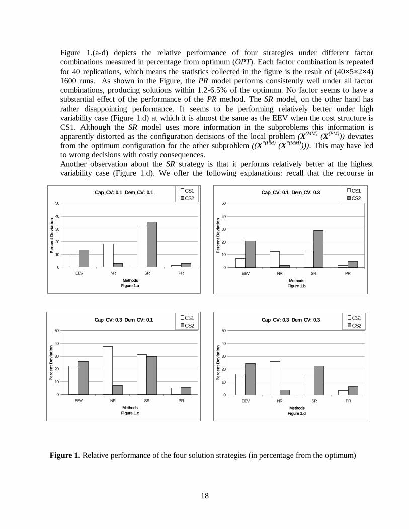
Figure 1.(a-d) depicts the relative performance of four strategies under different factor combinations measured in percentage from optimum (OPT). Each factor combination is repeated for 40 replications, which means the statistics collected in the figure is the result of (40×5×2×4) 1600 runs. As shown in the Figure, the PR model performs consistently well under all factor combinations, producing solutions within 1.2-6.5% of the optimum. No factor seems to have a substantial effect of the performance of the PR method. The SR model, on the other hand has rather disappointing performance. It seems to be performing relatively better under high variability case (Figure 1.d) at which it is almost the same as the EEV when the cost structure is CS1. Although the SR model uses more information in the subproblems this information is apparently distorted as the configuration decisions of the local problem (X(MM) (X(PM))) deviates from the optimum configuration for the other subproblem ((X*(PM) (X*(MM)))). This may have led to wrong decisions with costly consequences. Another observation about the SR strategy is that it performs relatively better at the highest variability case (Figure 1.d). We offer the following explanations: recall that the recourse in

Cap_CV: 0.1 Dem_CV: 0.1

0

10

20

30

40

50

EEV NR SR PR

MethodsFigure 1.a

Per

cent

Dev

iatio

n

CS1CS2

Cap_CV: 0.1 Dem_CV: 0.3

0

10

20

30

40

50

EEV NR SR PR

MethodsFigure 1.b

Per

cent

Dev

iatio

n

CS1CS2

Cap_CV: 0.3 Dem_CV: 0.1

0

10

20

30

40

50

EEV NR SR PR

MethodsFigure 1.c

Per

cent

Dev

iatio

n

CS1CS2

Cap_CV: 0.3 Dem_CV: 0.3

0

10

20

30

40

50

EEV NR SR PR

MethodsFigure 1.d

Per

cent

Dev

iatio

n

CS1CS2

Figure 1. Relative performance of the four solution strategies (in percentage from the optimum)

19

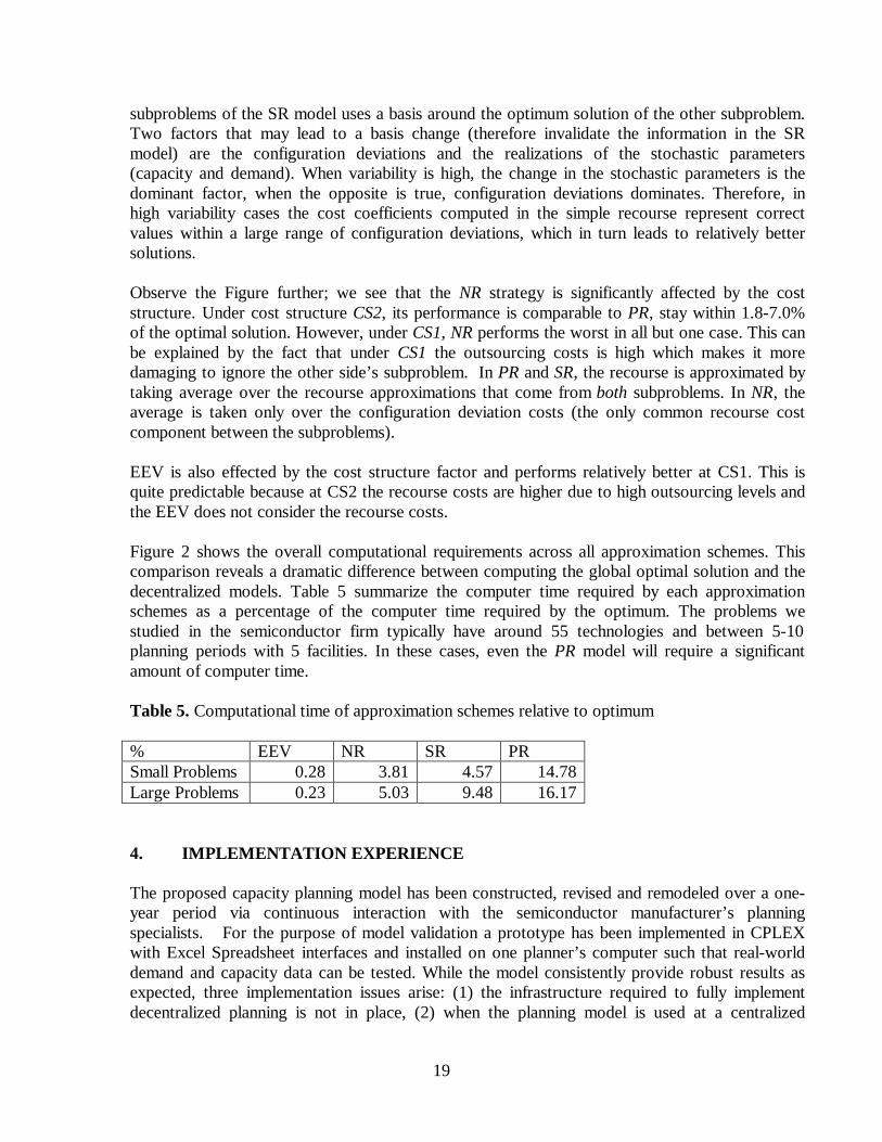
subproblems of the SR model uses a basis around the optimum solution of the other subproblem. Two factors that may lead to a basis change (therefore invalidate the information in the SR model) are the configuration deviations and the realizations of the stochastic parameters (capacity and demand). When variability is high, the change in the stochastic parameters is the dominant factor, when the opposite is true, configuration deviations dominates. Therefore, in high variability cases the cost coefficients computed in the simple recourse represent correct values within a large range of configuration deviations, which in turn leads to relatively better solutions. Observe the Figure further; we see that the NR strategy is significantly affected by the cost structure. Under cost structure CS2, its performance is comparable to PR, stay within 1.8-7.0% of the optimal solution. However, under CS1, NR performs the worst in all but one case. This can be explained by the fact that under CS1 the outsourcing costs is high which makes it more damaging to ignore the other side’s subproblem. In PR and SR, the recourse is approximated by taking average over the recourse approximations that come from both subproblems. In NR, the average is taken only over the configuration deviation costs (the only common recourse cost component between the subproblems). EEV is also effected by the cost structure factor and performs relatively better at CS1. This is quite predictable because at CS2 the recourse costs are higher due to high outsourcing levels and the EEV does not consider the recourse costs. Figure 2 shows the overall computational requirements across all approximation schemes. This comparison reveals a dramatic difference between computing the global optimal solution and the decentralized models. Table 5 summarize the computer time required by each approximation schemes as a percentage of the computer time required by the optimum. The problems we studied in the semiconductor firm typically have around 55 technologies and between 5-10 planning periods with 5 facilities. In these cases, even the PR model will require a significant amount of computer time. Table 5. Computational time of approximation schemes relative to optimum % EEV NR SR PR Small Problems 0.28 3.81 4.57 14.78 Large Problems 0.23 5.03 9.48 16.17 4. IMPLEMENTATION EXPERIENCE The proposed capacity planning model has been constructed, revised and remodeled over a one-year period via continuous interaction with the semiconductor manufacturer’s planning specialists. For the purpose of model validation a prototype has been implemented in CPLEX with Excel Spreadsheet interfaces and installed on one planner’s computer such that real-world demand and capacity data can be tested. While the model consistently provide robust results as expected, three implementation issues arise: (1) the infrastructure required to fully implement decentralized planning is not in place, (2) when the planning model is used at a centralized

20

location in the headquarter the information requirement (local cost information in particular) for the stochastic model becomes very high, and (3) the planner needs more flexibility to insert “non-quantitative” planning preferences and constraints due to various practical insights (e.g., a certain customer insists on using a particular manufacturing facility). For these reasons, the scenario analysis embedded in the stochastic programming model can only serve as an off-line analysis tool, allowing the planner to contemplate long-term planning ramifications. In the mean time, a simplified deterministic version (similar to EEV) of the model was implemented using Microsoft Excel and solved using the enhanced Excel Solver. The input data is extracted from the corporate ERP and imported to the model via Access database. This process has been automated to a large extend using Visual Basic for Applications (VBA). This particular configuration allows the planner to constantly “twig” the input data so as to incorporate additional insights and planning preferences. On the other hand, the constant data feed allows up-to-date information to be used in the planning process with heavy planner intervention. A future step is to integrate the scenario model into the on-line planning process to generate robust capacity plans. However, this cannot be done until proper infrastructure is set up to allow direct planning involvement from geographically separated marketing and manufacturing decision makers. The recent development in web-centric ERP systems provides possible support for such implementation. 5. CONCLUSIONS In this study, we develop a strategic capacity-planning model for a major semiconductor manufacturer. Motivated by the decentralized nature of these decisions between marketing and manufacturing, we proposed alternative scenario approximation schemes based on various assumptions of information usage. These schemes vary in complexity and information requirements, thus providing unique insights on the trade-off between decentralization and solution quality. We conduct extensive experiments (1,600 runs not including the pilot experiments) to gain insight on the solution characteristics under different levels of scenario variability, cost structures, and decision environments; and at the same time evaluate the performance of different scenario approximation schemes.

Small Problems

0.1 1.1 1.44.5

30.2

0

5

10

15

20

25

30

35

EEV NR SR PR OPT

MethodsFigure 2.a

Ave

rage

CP

U ti

me

(Sec

onds

)

Large Problems

0.4 8.1 15.2 25.9

160.0

020406080

100120140160180

EEV NR SR PR OPTMethodsFigure 2b

Ave

rage

CP

U ti

me

(Sec

onds

)

Figure 2. Average computational requirements for the approximation schemes

21

We observe that demand and capacity variability has distinct effects on the optimum stochastic solution. Specifically, capacity uncertainty induces more capacity expansions whereas demand uncertainty induces a higher level of outsourcing. This observation provides insight on strategic capacity planning decisions in semiconductor industry as capacity expansion and outsourcing present distinctly different cost implications. Our experiment shows that substantial benefits can be achieved by using a stochastic programming model for strategic capacity-planning problem (as demonstrated by the compassion with EEV), and that decentralization of decisions to the manufacturing and marketing managers can be achieved with a somewhat minor tradeoff in total cost. The partial recourse (PR) scheme, although the most demanding in terms of information and computational requirements produces near-optimal solutions (within 6.5%) with a small fraction of the computer time (at 16.17%). On the other hand the NR scheme performs well under a specific cost structure where the outsourcing costs dominate. Considering the low information requirements of NR and its low computational requirements, it may be worthwhile to investigate more special cases where it performs well. The simple recourse scheme falling between NR and PR (in terms of complexity) produces rather disappointing results.

ACKNOWLEDGEMENT The research is supported, in part, by National Science Foundation Grants DMI-9732173, DMI-9634808 and a grant from Lucent Technologies. We are greatly in debt to Jonathan Green who documented the problem context and implementation status of this project.

REFERENCES Benders, J.F., 1962, "Partitioning Procedures for Solving Mixed Variables Programming Problems", Numer. Math., 4:238-252. Berman, O., and Ganz, Z., and Wagner, J.M., 1994, "A Stochastic Optimization Model for Planning Capacity Expansion in a Service Industry under Uncertain Demand", Naval Research Logistics, Vol. 41, pp. 545-564. Bienstock, D., and Shapiro, J.F., 1988, "Optimizing Resource Acquisition Decisions by Stochastic Programming", Management Science, Vol. 34, No.2. Birge, J.R., 1984, "Decomposition and Partitioning Methods for Multistage Linear Programs", Operations Research, Vol.33, No.5. ___ 1997, "Stochastic Programming Computation and Applications", Informs Journal on Computing, Vol.9, No.2. Birge, J. R., and Wets, R.J.B., 1986, "Designing Approximation Schemes for Stochastic Optimization Problems, in Particular for Stochastic Programs with Recourse", Mathematical Programming Study 27, pp. 54-102.

22

Birge, J.R., and Louveaux, Francois, 1997, Introduction to Stochastic Programming, Springer Series in Operations Research, Springer-Verlag, New York Burton, R.M., and Obel, B., 1980, "The Efficiency of the Price, Budget, and Mixed Approaches under Varying a Priori Information Levels for Decentralized Planning", Management Science, Vol. 26, No.4. ___ 1984, Designing efficient organizations : modelling and experimentation, Elsevier Science Pub. Co., New York, N.Y., U.S.A ___ 1995, "Mathematical Contingency Modeling For Organizational Design: Taking Stock", Design Models for Hierarchical Organizations: Computation Information and Decentralization, edited by R. Burton and B. Obel, Kluwer Academic Publishers. Carpentier, P., and Cohen, G., and Culioli, J.-V., 1996, "Stochastic Optimization of Unit Commitment: a New Decomposition Framework", IEEE Transactions on Power Systems, Vol. 11, No. 2. Christensen, J., and Obel, B., 1978, "Simulation of Decentralized Planning in Two Danish Organizations Using Linear Programming Decomposition", Management Science, Vol.24, No.15. Dantzig, G.B., 1955, "Linear Programming Under Uncertainty", Management Science, Vol.1, No.3 and 4, pp.197-206. Dantzig, G.B., and Wolfe, P., 1961, "The Decomposition Algorithm for Linear Programs", Econometrica, Vol. 29, No.4. Escudero, L. F., and Kamesam, P., and V., King, A., J., and Wets, R. J-B., 1993, "Production Planning via Scenario Modeling", Annals of Operations Research, 43, pp.311-335. Eppen, G.D., and Martin, R.K., and Schrage, L., 1989, "A Scenario Approach to Capacity Planning", Operations Research, Vol 37, No. 4. Kall, P. and Wallace, S.W., 1994, Stochastic Programming, Wiley-Interscience Series in Systems and Optimization. Louveaux, F., 1986, "Multistage Stochastic Programs with Block-Separable Recourse", Mathematical Programming Study 28, pp. 48-62. Prekopa, A., 1995, Stochastic Programming, Kluwer Academic Publishers, Dordrecht. Takriti, S., and Birge, J. R., and Long, E., 1996, "A stochastic Mode for the Unit Commitment Problem", IEEE Transactions on Power Systems, Vol. 11, No. 3. Wallace, S.W. and Yan, T., 1993, "Bounding Multistage Stochastic Programs from Above", Mathematical Programming, 61, pp.111-129.