COOPERATIVES AND BRAZILIAN AGRICULTURAL PRODUCTION: A SPATIAL ANALYSIS Área ANPEC: Área 11 - Economia Agrícola e do Meio Ambiente Mateus de Carvalho Reis Neves: Professor Adjunto do Departamento de Economia Rural, Universidade Federal de Viçosa (UFV), Viçosa, MG, Brasil. E-mail: [email protected] Lucas Siqueira de Castro: Professor do Departamento de Economia, Universidade Federal Rural do Rio de Janeiro (UFRRJ), Seropédica, RJ, Brasil. E-mail: [email protected] Carlos Otávio de Freitas: Professor do Departamento de Administração, Universidade Federal Rural do Rio de Janeiro (UFRRJ), Seropédica, RJ, Brasil. E-mail: [email protected] Resumo: Como importantes elos de ligação entre os produtores e o mercado, e respondendo direta ou indiretamente por relevante parte do Produto Interno Bruto agropecuário nacional, as cooperativas carecem de estudos que mensurem o quanto são capazes de influenciar a produção no meio rural, considerando as diferenças regionais brasileiras. Assim, com este trabalho visou-se avaliar a existência e a magnitude do efeito das cooperativas na produção agropecuária das regiões brasileiras. Para tanto, foi construída uma função de produção, tendo as cooperativas como um fator deslocador da função de produção, considerando correção espacial, em nível municipal, para as regiões brasileiras. Os resultados evidenciam dependência espacial nos dados utilizados, justificando a abordagem metodológica utilizada neste trabalho. Verificou-se efeito positivo do cooperativismo no Valor Bruto da Produção da agropecuária nos municípios das regiões Sudeste, Centro-Oeste e Sul, ao passo em que se notou influência restritiva da associação às cooperativas no Norte e Nordeste do país. Conclui-se, portanto, que a expansão do cooperativismo pelas regiões do país não foi um processo homogêneo, havendo ainda um longo caminho a ser percorrido para que se tenham níveis mais elevados de cooperação no meio rural brasileiro. Palavras-Chave: Cooperativismo; Econometria Espacial; Função de Produção. Abstract: Cooperatives are important linkages between producers and the market, responding directly or indirectly for a relevant portion of the agricultural gross domestic product. There is a lack of studies that measure how much cooperatives influence production in the rural environment, considering the Brazilian regional differences. Thus, the objective is to identify the influence of cooperatives in the agricultural production of Brazilian regions. Therefore, a production function considering cooperatives as one of its inputs was constructed, considering a spatial correction at the municipal level for the Brazilian regions. The results show that there is spatial dependence on the data used, justifying the methodological approach used in this work. There was a positive effect of cooperatives on the Gross Value of Agricultural Production in the municipalities of the Southeast, Center-West and South regions, while the restrictive influence of the cooperative association in the North and Northeast of the country was noted. It is concluded, therefore, that the expansion of cooperatives by the regions of the country was not a homogeneous process, and that there is still a long way to go in order to have higher levels of cooperation in the Brazilian countryside. Keywords: Cooperatives; Spatial Econometrics; Production Function. JEL: Q13, C21

Welcome message from author
This document is posted to help you gain knowledge. Please leave a comment to let me know what you think about it! Share it to your friends and learn new things together.
Transcript

COOPERATIVES AND BRAZILIAN AGRICULTURAL PRODUCTION: A SPATIAL
ANALYSIS
Área ANPEC: Área 11 - Economia Agrícola e do Meio Ambiente
Mateus de Carvalho Reis Neves: Professor Adjunto do Departamento de Economia Rural, Universidade
Federal de Viçosa (UFV), Viçosa, MG, Brasil. E-mail: [email protected]
Lucas Siqueira de Castro: Professor do Departamento de Economia, Universidade Federal Rural do Rio
de Janeiro (UFRRJ), Seropédica, RJ, Brasil. E-mail: [email protected]
Carlos Otávio de Freitas: Professor do Departamento de Administração, Universidade Federal Rural do
Rio de Janeiro (UFRRJ), Seropédica, RJ, Brasil. E-mail: [email protected]
Resumo:
Como importantes elos de ligação entre os produtores e o mercado, e respondendo direta ou indiretamente
por relevante parte do Produto Interno Bruto agropecuário nacional, as cooperativas carecem de estudos
que mensurem o quanto são capazes de influenciar a produção no meio rural, considerando as diferenças
regionais brasileiras. Assim, com este trabalho visou-se avaliar a existência e a magnitude do efeito das
cooperativas na produção agropecuária das regiões brasileiras. Para tanto, foi construída uma função de
produção, tendo as cooperativas como um fator deslocador da função de produção, considerando correção
espacial, em nível municipal, para as regiões brasileiras. Os resultados evidenciam dependência espacial
nos dados utilizados, justificando a abordagem metodológica utilizada neste trabalho. Verificou-se efeito
positivo do cooperativismo no Valor Bruto da Produção da agropecuária nos municípios das regiões
Sudeste, Centro-Oeste e Sul, ao passo em que se notou influência restritiva da associação às cooperativas
no Norte e Nordeste do país. Conclui-se, portanto, que a expansão do cooperativismo pelas regiões do país
não foi um processo homogêneo, havendo ainda um longo caminho a ser percorrido para que se tenham
níveis mais elevados de cooperação no meio rural brasileiro.
Palavras-Chave: Cooperativismo; Econometria Espacial; Função de Produção.
Abstract:
Cooperatives are important linkages between producers and the market, responding directly or indirectly
for a relevant portion of the agricultural gross domestic product. There is a lack of studies that measure
how much cooperatives influence production in the rural environment, considering the Brazilian regional
differences. Thus, the objective is to identify the influence of cooperatives in the agricultural production of
Brazilian regions. Therefore, a production function considering cooperatives as one of its inputs was
constructed, considering a spatial correction at the municipal level for the Brazilian regions. The results
show that there is spatial dependence on the data used, justifying the methodological approach used in this
work. There was a positive effect of cooperatives on the Gross Value of Agricultural Production in the
municipalities of the Southeast, Center-West and South regions, while the restrictive influence of the
cooperative association in the North and Northeast of the country was noted. It is concluded, therefore,
that the expansion of cooperatives by the regions of the country was not a homogeneous process, and that
there is still a long way to go in order to have higher levels of cooperation in the Brazilian countryside.
Keywords: Cooperatives; Spatial Econometrics; Production Function.
JEL: Q13, C21
COOPERATIVES AND BRAZILIAN AGRICULTURAL PRODUCTION: A SPATIAL
ANALYSIS
Área ANPEC: Área 11 - Economia Agrícola e do Meio Ambiente
Resumo:
Como importantes elos de ligação entre os produtores e o mercado, e respondendo direta ou indiretamente
por relevante parte do Produto Interno Bruto agropecuário nacional, as cooperativas carecem de estudos
que mensurem o quanto são capazes de influenciar a produção no meio rural, considerando as diferenças
regionais brasileiras. Assim, com este trabalho visou-se avaliar a existência e a magnitude do efeito das
cooperativas na produção agropecuária das regiões brasileiras. Para tanto, foi construída uma função de
produção, tendo as cooperativas como um fator deslocador da função de produção, considerando correção
espacial, em nível municipal, para as regiões brasileiras. Os resultados evidenciam dependência espacial
nos dados utilizados, justificando a abordagem metodológica utilizada neste trabalho. Verificou-se efeito
positivo do cooperativismo no Valor Bruto da Produção da agropecuária nos municípios das regiões
Sudeste, Centro-Oeste e Sul, ao passo em que se notou influência restritiva da associação às cooperativas
no Norte e Nordeste do país. Conclui-se, portanto, que a expansão do cooperativismo pelas regiões do país
não foi um processo homogêneo, havendo ainda um longo caminho a ser percorrido para que se tenham
níveis mais elevados de cooperação no meio rural brasileiro.
Palavras-Chave: Cooperativismo; Econometria Espacial; Função de Produção.
Abstract:
Cooperatives are important linkages between producers and the market, responding directly or indirectly
for a relevant portion of the agricultural gross domestic product. There is a lack of studies that measure
how much cooperatives influence production in the rural environment, considering the Brazilian regional
differences. Thus, the objective is to identify the influence of cooperatives in the agricultural production of
Brazilian regions. Therefore, a production function considering cooperatives as one of its inputs was
constructed, considering a spatial correction at the municipal level for the Brazilian regions. The results
show that there is spatial dependence on the data used, justifying the methodological approach used in this
work. There was a positive effect of cooperatives on the Gross Value of Agricultural Production in the
municipalities of the Southeast, Center-West and South regions, while the restrictive influence of the
cooperative association in the North and Northeast of the country was noted. It is concluded, therefore,
that the expansion of cooperatives by the regions of the country was not a homogeneous process, and that
there is still a long way to go in order to have higher levels of cooperation in the Brazilian countryside.
Keywords: Cooperatives; Spatial Econometrics; Production Function.
JEL: Q13, C21

1. Introduction
Cooperatives1 in rural areas primarily comprise farmers seeking to alleviate the anxiety associated with
their activities. In Brazil, according to data taken from the last Agricultural Census, approximately 41% of
the gross value of agricultural and livestock production (GVP) passes through a cooperative (IBGE, 2016).
Thus, cooperatives coordinate the activities of actors in the primary sector of the economy and provide
important market access routes.
Although relevant in terms of agriculture, few studies assess the influence of agricultural and livestock
cooperatives in Brazil from economic or production perspectives. Internationally, authors such as
McNamara et al. (2001), Folsom (2003), Zeuli et al. (2003), Zeuli and Deller (2007), Rodrigo (2012),
Cazzuffi (2013), and Jardine et al. (2014) have evaluated the economic effects of cooperatives in rural
areas. These studies consider the impacts of cooperatives on, among other things, the value of production
and the gross domestic product (GDP)2. However, none consider cooperatives in the context of Brazilian
agriculture.
Studies on cooperativism in Brazilian agriculture need to consider the characteristics of regions, as
reflected in the rural environment. The findings of studies by, for example, Helfand and Brunstein (2001),
Silva et al. (2003), FGV (2010), Kageyama et al. (2013), Helfand et al. (2014), and Belik (2015) reinforce
the differences in productive patterns and the inequalities in agricultural areas. Such inequalities are not
restricted to the large property versus small property dichotomy. Profound heterogeneity exists even among
the smaller establishments in the various regions of Brazil.
Therefore, in this study, we examine the influence of cooperatives on agricultural production in
Brazilian regions, which is markedly heterogeneous in terms of production, socioeconomic factors, and
“social capital”, in the sense shown by Putnam (1995). Given this objective, we employ a production
function that includes spatial corrections, and takes inputs commonly used in rural production, considering
the cooperatives and its influence in the productive process.
The article consists of four sections besides this introduction. In the second section, we briefly discuss
the cooperativism in the Brazilian agricultural sector. In the third section, we present the empirical strategy
used, and the data source. In the fourth section, we bring the discussion about the results. Finally, the fifth
section deals with the final considerations about the established problem.
2. Cooperativism in Rural Brazil: Relevance and Heterogeneity
The literature on the economics of organizations explains the existence of agricultural cooperatives in
terms of their ability to: a) generate economies of scale; b) access new markets, including international
markets; c) reduce costs through vertical integration; d) reduce risks in joint actions; e) enable members to
access and adopt technologies and inputs through technical assistance services; f) provide members with
greater bargaining power to obtain better prices; and g) dilute the risk of economic activities by undertaking
joint actions (Bonus, 1986; Sexton, 1986; Staatz, 1987; Hansmann, 1988, 1996; Sexton and Iskow, 1988;
Bialoskorski Neto, 2000; Valentinov, 2007).
These characteristics explain the spread of cooperativism in several countries. In Japan, agricultural
cooperatives include around 90% of all farmers, while in Canada and Norway, 4 out of 10 farmers are
members of cooperatives. Furthermore, in New Zealand, cooperatives account for 95% of the dairy market
and 22% of GDP (Namorado, 2013).
In Brazil, the use of the cooperative model dates back to the end of the 19th century in the states of São
Paulo and Pernambuco. In 1902, the first rural credit cooperative (or credit unions) of the Raiffeisen model
emerged (Nova Petrópolis, RS), followed in 1907 by the first agricultural cooperative (Minas Gerais).
During the first half of the 20th century, these were the most relevant agricultural cooperatives in terms of
1 Although the word “cooperative” can be applied to different types of collectively developed activities, we use the term to
describe a democratically controlled and managed business model. In many countries, as in Brazil, cooperatives are defined
legally as a specific type of corporation, and are subject to specific federal legislation (Zeuli and Radel, 2005). 2 Similar works can be found in Zeuli and Deller (2007) and Uzea and Duguid (2015). Both analyze the nuances of the economic
impact of cooperatives, highlighting the methodologies used in such studies.
volume of business, and were largely responsible for the diffusion of the cooperative ideology throughout
the country (Silva et al., 2003).
Pinho (1996) and Presno (2001) assert that cooperatives were fomented by the government since the
1930s as instruments for the application and dissemination of public policies oriented to the agrarian sector
(e.g., technical assistance, market access, etc.). However, no prior studies have examined the sustainability
of most cooperatives created as a result of these policies. Additionally, the 1980s were characterized by a
slowdown in national economic activity and state interventionist policies, coupled with growing demand
for more modern management practices. These factors led to the disappearance of many agricultural
cooperatives, as well as a growing fear of such organizations (Pinho, 1992; Presno, 2001; Bialoskorski
Neto, 2005).
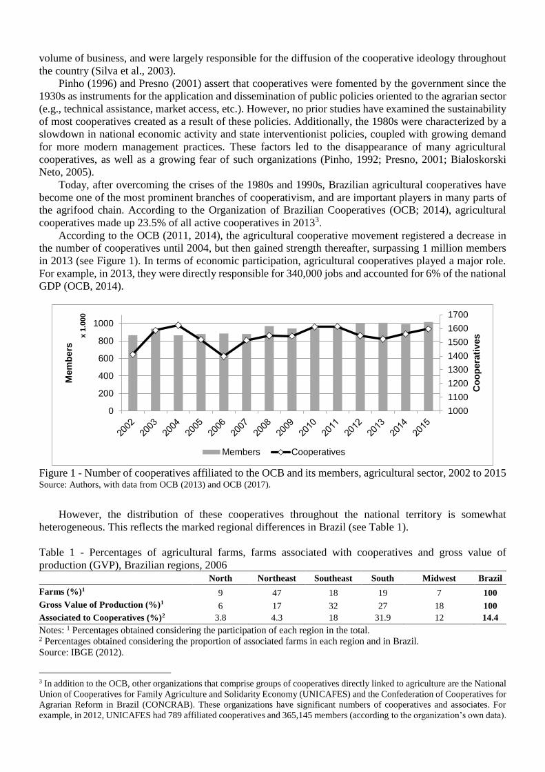
Today, after overcoming the crises of the 1980s and 1990s, Brazilian agricultural cooperatives have
become one of the most prominent branches of cooperativism, and are important players in many parts of
the agrifood chain. According to the Organization of Brazilian Cooperatives (OCB; 2014), agricultural
cooperatives made up 23.5% of all active cooperatives in 20133.
According to the OCB (2011, 2014), the agricultural cooperative movement registered a decrease in
the number of cooperatives until 2004, but then gained strength thereafter, surpassing 1 million members
in 2013 (see Figure 1). In terms of economic participation, agricultural cooperatives played a major role.
For example, in 2013, they were directly responsible for 340,000 jobs and accounted for 6% of the national
GDP (OCB, 2014).
Figure 1 - Number of cooperatives affiliated to the OCB and its members, agricultural sector, 2002 to 2015 Source: Authors, with data from OCB (2013) and OCB (2017).
However, the distribution of these cooperatives throughout the national territory is somewhat
heterogeneous. This reflects the marked regional differences in Brazil (see Table 1).
Table 1 - Percentages of agricultural farms, farms associated with cooperatives and gross value of
production (GVP), Brazilian regions, 2006 North Northeast Southeast South Midwest Brazil
Farms (%)1 9 47 18 19 7 100
Gross Value of Production (%)1 6 17 32 27 18 100
Associated to Cooperatives (%)2 3.8 4.3 18 31.9 12 14.4
Notes: 1 Percentages obtained considering the participation of each region in the total. 2 Percentages obtained considering the proportion of associated farms in each region and in Brazil.
Source: IBGE (2012).
3 In addition to the OCB, other organizations that comprise groups of cooperatives directly linked to agriculture are the National
Union of Cooperatives for Family Agriculture and Solidarity Economy (UNICAFES) and the Confederation of Cooperatives for
Agrarian Reform in Brazil (CONCRAB). These organizations have significant numbers of cooperatives and associates. For
example, in 2012, UNICAFES had 789 affiliated cooperatives and 365,145 members (according to the organization’s own data).
1000
1100
1200
1300
1400
1500
1600
1700
0
200
400
600
800
1000
Co
op
era
tiv
es
Mem
bers
x 1
.000
Members Cooperatives

According to data taken from the 2006 Agricultural Census, on average, 14.4% of farms were
associated with cooperatives. In addition, there is an evident disparity between the Brazil regions, not only
in terms of the consolidation of the cooperative movement, but also in terms of the number of farms and
the agricultural GVP. According to Helfand and Brunstein (2001), these regional differences are recurrent
in analyses of Brazilian agriculture. This reflects the diverse conditions in the infrastructure, labor market,
and distances from consumer centers and other points, as well as case-specific cooperation, cultural, and
historical issues.
In 2006, only 3.8% of the rural establishments in the North Region were associated with cooperatives.
In the Northeast, where a little over 4% of the establishments were associated with cooperatives, there was
a significant contrast between the proportion of establishments (47%) and their participation in the GVP
(17%). In contrast, the South and Southeast Regions had the highest percentages of establishments
associated with cooperatives (31.9% and 18%, respectively). These two regions also showed the highest
participation in the gross value of agricultural production (GVP), leading to the question of whether, in fact,
cooperatives aid the production of agricultural establishments.
Although it does not completely explain the magnitude, these regional differences in Brazilian
cooperativism were strongly influenced by immigrants. Germans, Italians, and Japanese settled in the South
and Southeast Regions. Many of these immigrants had some experience with associativism, instilling the
culture, cooperative education, and high level of social capital4 necessary to serve as a foundation for a
competitive cooperativism structure (Silva et al., 2003). In addition, governmental aid contributed to these
regional discrepancies, with the greatest flow in recent decades going to the Southeast Region (Duarte,
1986).
3. Empirical Strategy
3.1. Production Function
We employ a generic production functional relationship, 𝑌 = 𝑓(𝑊, 𝐿, 𝐾 … ), as described in Humphrey
(1997), where Y is the output resulting from the combination of the factors of work W, land L, capital K,
and so on, and adapt it to the objective of this work, as follows:
𝑌𝑖 = 𝑓(𝑊𝑖, 𝐿𝑖 , 𝐼𝑖, 𝐾𝑖, 𝐶𝑖), (1)
where 𝑌𝑖 is the gross value of agricultural production, 𝑊𝑖 refers to the work units used, 𝐿𝑖 is the cultivated
area (in hectares), 𝐼𝑖 represents the amount spent on inputs (in USD5), 𝐾𝑖 refers to farm buildings (in USD),
and 𝐶𝑖 is the proportion of farmers who are members of cooperatives. These variables all refer to the
agricultural establishments in municipality i.
The cooperatives 𝐶𝑖 in this function are not a direct factor of production, but act as dislocators of the
production function6. For example, they would allow rural producers access to new inputs and markets. As
defined by Curi (1997), investments in access to information, modern industrial parks, technical assistance,
and rural extensions can be understood as modernizing agriculture, promoting these elements and leading
to changes in the level of Brazilian agriculture.
The theoretical adequacy of this functional relationship was proposed by Cobb and Douglas (1928).
The Cobb–Douglas functional form is commonly used because it is a simple model with a restricted number
of properties, such as elasticity and constant returns to scale (Coelli et al., 1998). Acording to Baumol
(1977) and Castro (2002), despite its limitations, the Cobb–Douglas specification provides results that are
easy to interpret (the estimated coefficients are the model’s own elasticity), as well as good statistical
qualities in terms of adherence to the data. The model is also useful in the estimation process, because it
becomes linear when rewritten using the logarithmic form of each variable:
4 As defined in Putnam (1995), this capital is a coalition of elements, namely, trust, reciprocity, social cohesion, and civism. 5 The average exchange rate in 2006 was R$2.17/USD. 6 Here, we perform a cross-sectional analysis, based on the importance of technology, as in the innovation model induced by
Hayami and Ruttan (1971), where technology is as an endogenous variable in the process of production growth.
𝑙𝑛𝑌𝑖 = 𝑙𝑛𝐴 + 𝛼𝑙𝑛𝑊𝑖 + 𝛽1𝑙𝑛𝐿𝑖 + 𝛽2𝑙𝑛𝐼𝑖 + 𝛽3𝑙𝑛𝐾𝑖 + 𝛽4𝑙𝑛𝐶𝑖. (2)
This function minimizes the number of coefficients to be estimated and avoids possible
multicollinearity problems. Then, we add the spatial characteristics of the final model used in this work to
the function. Because the perspectives involve geographical disaggregation at the municipal level, we
consider the possibility of spatial dependence between the regions. In other words, a municipality might be
affected by the characteristics of neighboring municipalities, and vice versa, which would make it
impossible to interpret the results from the ordinary least squares (OLS) method.
3.2. Spatial Aspects
The first step in the investigation is an exploratory spatial data analysis (ESDA). The ESDA uses
Moran’s I, which considers both global and local perspectives on the variables.
The second step is a conventional estimation of the models using the OLS method. Here, the Moran
test is also applied to the residual values of the MQO model in order to verify the existence of spatial
autocorrelation. If found, the model developed in the third step needs to eliminate this problem by including
spatial lags/interactions. More specific tests, such as the Lagrange multiplier and its robust versions, are
used to identify the type of spatial lag to be included in the estimated model7.
The final specification of the spatial model is given in equations (3a) and (3b):
𝑦𝑖𝑡 = 𝛼 + 𝜌𝑊𝑦𝑖𝑡 + 𝑋𝑖𝑡𝛽 + 𝑊𝑋𝑖𝑡𝜏 + 𝜉𝑖𝑡 (3a)
𝜉𝑖𝑡 = 𝜆𝑊𝜉𝑖𝑡 + 𝜀𝑖𝑡, (3b)
where 𝜏, 𝜌, and 𝜆 are coefficients to be estimated; y represents the dependent variable, namely, the gross
value of agricultural production; X is a vector of the control variables defined in the previous subsection;
W denotes the spatial weighting matrices; and 𝜉 corresponds to the error term.
Imposing restrictions on the spatial parameters of equation (3), we determine several spatial models.
For 𝜏 = 𝜆 = 0 and 𝜌 ≠ 0, we obtain the SAR model. For 𝜏 = 𝜌 = 0 and 𝜆 ≠ 0, we have the SEM mode.
For 𝜆 = 0, 𝜏 ≠ 0, and 𝜌 ≠ 0, we obtain the SDM model. For 𝜌 = 0, 𝜏 ≠ 0, and 𝜆 ≠ 0, we have the SDEM
model, and for 𝜌 = 𝜆 = 0 and 𝜏 ≠ 0, we have the SLX model8.
In addition to information on given contiguous areas, spatial models generate coefficients of partial
correlations between variables. LeSage and Pace (2009) show that it is possible to divide these coefficients
as direct, indirect, and total effects. For this, it is necessary that the spatial dependence be observable, as in
the SAR, SDM, and SLX models. If this is possible, using the technique increases the quality of the
information on the influence of cooperatives on agricultural production in the various regions of Brazil.
3.3 Data
The data used in this study are taken from the 2006 Brazilian Agricultural Census, the last year of this
study in Brazil (IBGE, 2016). The Census covered the period January 1 to December 31, 2006, and provides
cross-sectional data (IBGE, 2012). Note that the model discussed in the previous sections is not estimated
using farm-level data.
The results of the 2006 Agricultural Census are disclosed at the level of administrative units (i.e.,
municipalities) in order to aggregate agricultural establishments. This aggregation preserves the identities
of farmers. Therefore, the basic unit of analysis of the data used for the operationalization of the restricted
profit function are farms, aggregated by municipalities in the Brazilian macro-regions.
Considering the 5,500 municipalities that make up the units of analysis, we assume that this is the
maximum number of observations. According to Helfand et al. (2015), the aggregation of the data leads to
7 The literature lists other procedures that facilitate the estimation of spatial models. Among the commonly employed there are
the classic, the hybrid, the Hendry (Florax et al., 2003) and the complete (Almeida, 2012). 8 If the spatial parameters of equation (3) are null, the model obtained is the conventional OLS.
an assumption of homogeneity between the observations. Here, each of the 5,500 “representative farms“9
reflect the average behavior of a group of individual farms in a given municipality. These 5,500
municipalities encompass 5,175,636 farms, according to data taken from the IBGE (2016).
To estimate the production function, the GVP in 2006 (production), in USD, is defined as the output
variable. The factors of production are defined by the following variables: a) productive area (land, in
hectares (ha)), as the sum of the areas used for agriculture, livestock, and agroforestry, used as a proxy of
the land factor; b) total value (in USD), of farm goods (capital), used as a proxy for capital goods; c) the
sum of the number of family work units (wu) and contracted workers (work)10, used as a proxy for the work
factor; and d) non-productive expenditure (inputs), which is the sum (in USD) of expenses related to soil
correctives, fertilizers, pesticides, animal medicines, seeds and seedlings, salt/feed, fuel, and energy, used
as a proxy for the inputs.
The variable of interest, cooperative membership, is used here based on evidence that these
organizations can influence the optimal choices of rural producers. Thus, an important issue in this work is
finding a way to represent this variable. Because the 2006 Agricultural Census does not provide micro-
level data, one alternative is to consider the percentage of farmers who answered “yes” to the question,
“Are you a member of a cooperative?” Therefore, this variable is represented by the proportion of all farms
in each municipality that provided positive responses.
In Brazil, cooperativism is strongly influenced by the Rochdale Principles11, from the first legislation
on cooperatives to the “Cooperative Law” of 1971, as noted by Pinho (1992). Thus, by legal imposition,
cooperatives have free entry, except for technical limitations on accepting additional members. Similarly,
there is no restriction on the departure of members. However, in order for a rural producer to be part of a
cooperative, he must live in the region where the cooperative operates and must contribute to capital. Thus,
the decision to join a cooperative by a rural producer is complex and involves several factors: the
availability of cooperatives and other capital companies offering equivalent services, prices, and cultural
and historical aspects. These factors all influence the number of rural producers who opt to join a
cooperative.
It is important to consider the regional differences of Brazil when analyzing the production function
for the municipalities. According to Buainain et al. (2007), in addition to the natural conditions, the
Brazilian territory is heterogeneous by other factors, such as those related to the historical process of
colonization. With this in mind, the regression is estimated by considering fixed effects at regional levels
in an attempt to control this spatial heterogeneity. To do so, the variable of interest was being regressed on
dummies for each macro-region of the country (North (DN), Northeast (DNE), Southeast (DSE), and
Central–West (DMW), with the South region as base category). The dummy variables take the value one
when the municipality belongs to a unit of the federation, and zero otherwise. Thus, these variables are
included in the model to represent the level of cooperative membership in the municipalities of each region
in Brazil.
Note that all aggregations, data generation, and analyses are carried out using STATA®, Geoda®,
GeodaSpace®, and R.
4. Results
4.1. Descriptive Statistics
9 For a discussion of the consequences of using “representative farms” in rural economy studies, refer to Nerlove and Bachman
(1960), Barker and Stanton (1965), and Sharples (1969). 10 According to the methodology of the 2006 Brazilian Agricultural Census, the family work unit (wu) is calculated as the sum
of the number of persons, men or women, 14 years of age or older and with ties of kinship (including the person who runs the
farm), more than half the number of persons with ties of kinship and who are under the age of 14, the number of employees in
“other ” condition aged 14 years or over, and half the number of employees in the “other” condition under the age of 14 years.
The contracted work unit is the sum of the number of men and women who are permanent employees and 14 years of age or
older, half the number of permanent employees under the age of 14 years, partner employees over the age of 14 years, and half
the number of employees younger than 14 years of age, plus the result of dividing the number of days paid in 2006 by 260, and
that of dividing the days of work by 260 (IBGE, 2012). 11 In 1966, on the occasion of the Congress of the International Cooperative Alliance in Vienna, the “Principles” of the Rochdale
Pioneers (first cooperative, created in this British district) were established.
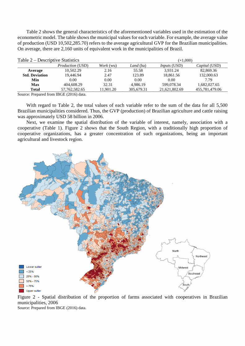
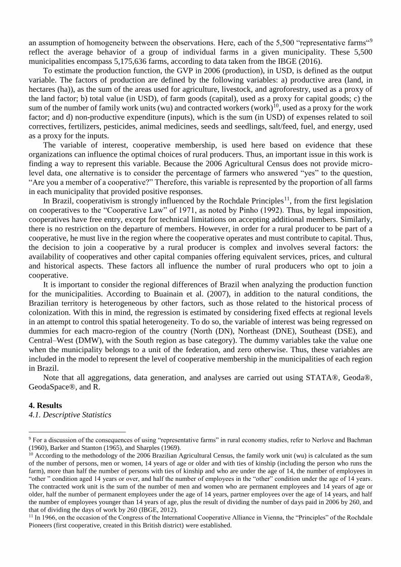
Table 2 shows the general characteristics of the aforementioned variables used in the estimation of the
econometric model. The table shows the municipal values for each variable. For example, the average value
of production (USD 10,502,285.70) refers to the average agricultural GVP for the Brazilian municipalities.
On average, there are 2,160 units of equivalent work in the municipalities of Brazil.
Table 2 – Descriptive Statistics (×1,000) Production (USD) Work (wu) Land (ha) Inputs (USD) Capital (USD)
Average 10,502.29 2.16 55.58 3,931.24 82,869.36
Std. Deviation 19,446.94 2.47 123.89 18,861.56 132,000.63
Min 0.00 0.00 0.00 0.00 7.79
Max 404,608.29 32.31 4,986.19 599,078.34 1,682,027.65
Total 57,762,582.65 11,901.20 305,679.31 21,621,802.69 455,781,479.06
Source: Prepared from IBGE (2016) data.
With regard to Table 2, the total values of each variable refer to the sum of the data for all 5,500
Brazilian municipalities considered. Thus, the GVP (production) of Brazilian agriculture and cattle raising
was approximately USD 58 billion in 2006.
Next, we examine the spatial distribution of the variable of interest, namely, association with a
cooperative (Table 1). Figure 2 shows that the South Region, with a traditionally high proportion of
cooperative organizations, has a greater concentration of such organizations, being an important
agricultural and livestock region.
Figure 2 - Spatial distribution of the proportion of farms associated with cooperatives in Brazilian
municipalities, 2006 Source: Prepared from IBGE (2016) data.

In the Southeast Region, which has an average of 18% of agricultural establishments associated with
cooperatives, there is a concentration of municipalities with a proportion of members above 0.20 in the
state of Minas Gerais and in the state of São Paulo. Then, Goiás and Mato Grosso do Sul also have high
proportions of establishments in cooperatives in the Central–West Region, which has a lower concentration
of municipalities and high rates of association with cooperatives. In the municipalities of the North and
Northeast of the country, it is clear that most of these belong to the lower quantiles of rates of association
with cooperatives (Ceará, Maranhão, Piauí, Amazonas, and Roraima).
4.2. Spatial Data Analysis
The exploratory spatial data analysis (ESDA) performed on the dependent and control variables is
divided into two parts: global and local. In both analyses, it was necessary to determine the most appropriate
types of spatial weighting matrices (W). The choice of matrices for these procedures is based on the
procedure proposed in Baumont (2004)12.
In the overall evaluation, the matrices chosen were those of type k neighbors. The grading of the
matrices per variable is shown in Table 3, which also shows the results of the Moran test. In general,
regardless of the variable analyzed, the p-values are statistically significant at the 1% level, which indicates
the existence of spatial patterns in the variables selected at the municipal level for Brazil.
Table 3 - Moran's I statistics for the dependent and control variables
Matrixes Variable Values Average Std. Deviation Z p-values
k-4 capital 0.4115 0.0000 0.0090 45.9204 0.0000***
k-7 work 0.3190 0.0000 0.0068 46.6213 0.0000***
k-2 cooperatives 0.7876 0.0000 0.0124 63.7351 0.0000***
k-2 land 0.4337 0.0000 0.0124 35.0992 0.0000***
k-5 production 0.2264 0.0000 0.0081 28.1154 0.0000***
k-3 inputs 0.1282 0.0000 0.0103 12.5167 0.0000***
Source: Prepared by the authors.
Note: * Significant at the 10% level; ** Significant at the 5% level; *** Significant at the 1% level.
Indicating the existence of spatial autocorrelation, the results also provide clues on determining how
these patterns manifest themselves. Signals of the coefficients indicate the presence of positive spatial
dependence, which configures geographic concentration by two modes. In the first, municipalities with
high production values, for example, will make border with municipalities with similar values. In the
second, municipalities with low land values will be contiguous with municipalities with similar
characteristics.
The local research is conducted using local indicator of spatial association (LISA) maps, operating
nearby k-2 matrices. In this case, we chose the mapping for the variable of interest (association to
cooperatives) only, as shown in Figure 3. This analysis allows us to observe the majority of the two types
of clusters (high–high and low–low), in addition to several municipalities whose indicators of local spatial
autocorrelation are not statistically significant.
The high–high clusters indicate municipalities and neighboring municipalities with high rates of
association with cooperatives (above average). This cluster is concentrated in the Southeast, South, and
Central–West Regions, historically marked by the existence of a greater number of farms associated with
cooperatives. Strong and comprehensive cooperatives operating in the headquarters and adjacent
municipalities are common in the South Region, primarily in the states of Paraná and Santa Catarina, as
well as in the milk supply cooperatives of the Southeast (Neves and Braga, 2014). Added to this is the
important role of credit unions in providing credit to many rural producers in these regions.
On the other hand, clusters of the low–low type are located in the North and Northeast, with the greater
quantity being in the latter region. These are regions where cooperativism is still not as widespread as it is
12 The procedure is to perform spatial autocorrelation tests, such as Moran’s I, on OLS residual values. The option for the matrix
is chosen based on the test result with the largest statistically significant spatial autocorrelation. Thus, the Baumont (2004)
procedure prevents the existence of bias associated with the way the spatial matrices are selected.
in the Central–West and South Regions of Brazil. This pattern is very similar to that established by the
spatial dispersion of Figure 2.
Figure 3 - LISA cluster map for the variable of interest (cooperative membership), 2006. Source: Prepared by the authors.
4.3. Effect of cooperative membership
Following the analysis proposed in the empirical strategy, the model was initially estimated using the
OLS approach (see Table 4)13. The results reported in the second column (OLS model) show that all control
variables are statistically significant at the 1% level. This includes the dummies that capture the regional
membership rate of cooperatives. However, a verification of the diagnostic tests reveals traces of spatial
dependence. This confirms the results of the ESDA, just as the residual values were heteroscedastic and
non-normal. Thus, as predicted, the OLS model proved to be poorly specified, which makes it impossible
to interpret its coefficients.
In order to expand the types of spatial autocorrelation, we perform Lagrange multiplier tests for the lag
(MLρ) and for the autoregressive error (MLλ). These tests were all statistically different from zero, which
suggests, preliminarily, that the spatial model of interest may be one of SAR, SEM, SDM, or SDEM.
To determine the most adequate of the suggested models, we apply the method of Stakhovych and
Bijmolt (2009). This criterion compares the Akaike statistics provided by the estimated models, which use
different spatial lag matrices. The best choice is the model that presents the lowest Akaike value and that,
at the same time, eliminates the problem of spatial dependence.
13 Note that for the estimation of the econometric models, we interpolate the interest variable (cooperative member rate) using
dummies for each region of Brazil (DN, DNE, DSE, and DMW, with the South Region as the base category).
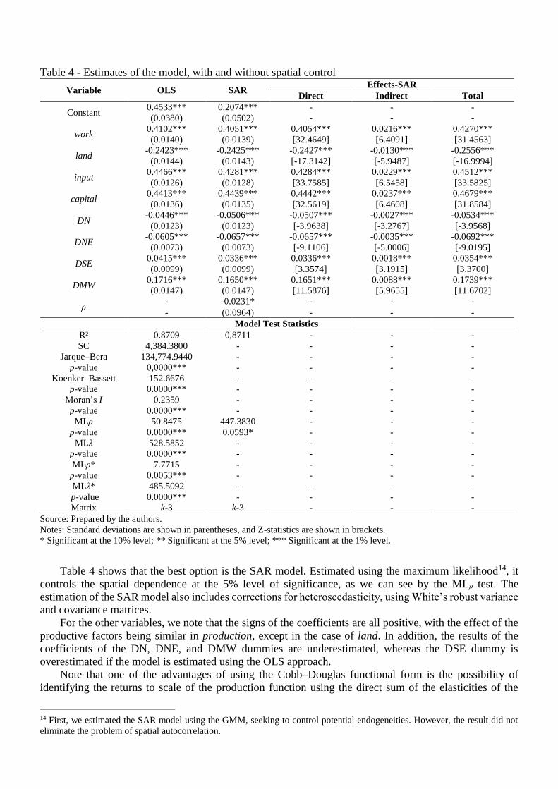
Table 4 - Estimates of the model, with and without spatial control
Variable OLS SAR Effects-SAR
Direct Indirect Total
Constant 0.4533*** 0.2074*** - - -
(0.0380) (0.0502) - - -
work 0.4102*** 0.4051*** 0.4054*** 0.0216*** 0.4270***
(0.0140) (0.0139) [32.4649] [6.4091] [31.4563]
land -0.2423*** -0.2425*** -0.2427*** -0.0130*** -0.2556***
(0.0144) (0.0143) [-17.3142] [-5.9487] [-16.9994]
input 0.4466*** 0.4281*** 0.4284*** 0.0229*** 0.4512***
(0.0126) (0.0128) [33.7585] [6.5458] [33.5825]
capital 0.4413*** 0.4439*** 0.4442*** 0.0237*** 0.4679***
(0.0136) (0.0135) [32.5619] [6.4608] [31.8584]
DN -0.0446*** -0.0506*** -0.0507*** -0.0027*** -0.0534***
(0.0123) (0.0123) [-3.9638] [-3.2767] [-3.9568]
DNE -0.0605*** -0.0657*** -0.0657*** -0.0035*** -0.0692***
(0.0073) (0.0073) [-9.1106] [-5.0006] [-9.0195]
DSE 0.0415*** 0.0336*** 0.0336*** 0.0018*** 0.0354***
(0.0099) (0.0099) [3.3574] [3.1915] [3.3700]
DMW 0.1716*** 0.1650*** 0.1651*** 0.0088*** 0.1739***
(0.0147) (0.0147) [11.5876] [5.9655] [11.6702]
ρ - -0.0231* - - -
- (0.0964) - - -
Model Test Statistics
R² 0.8709 0,8711 - - -
SC 4,384.3800 - - - -
Jarque–Bera 134,774.9440 - - - -
p-value 0,0000*** - - - -
Koenker–Bassett 152.6676 - - - -
p-value 0.0000*** - - - -
Moran’s I 0.2359 - - - -
p-value 0.0000*** - - - -
MLρ 50.8475 447.3830 - - -
p-value 0.0000*** 0.0593* - - -
MLλ 528.5852 - - - -
p-value 0.0000*** - - - -
MLρ* 7.7715 - - - -
p-value 0.0053*** - - - -
MLλ* 485.5092 - - - -
p-value 0.0000*** - - - -
Matrix k-3 k-3 - - -
Source: Prepared by the authors.
Notes: Standard deviations are shown in parentheses, and Z-statistics are shown in brackets.
* Significant at the 10% level; ** Significant at the 5% level; *** Significant at the 1% level.
Table 4 shows that the best option is the SAR model. Estimated using the maximum likelihood14, it
controls the spatial dependence at the 5% level of significance, as we can see by the MLρ test. The
estimation of the SAR model also includes corrections for heteroscedasticity, using White’s robust variance
and covariance matrices.
For the other variables, we note that the signs of the coefficients are all positive, with the effect of the
productive factors being similar in production, except in the case of land. In addition, the results of the
coefficients of the DN, DNE, and DMW dummies are underestimated, whereas the DSE dummy is
overestimated if the model is estimated using the OLS approach.
Note that one of the advantages of using the Cobb–Douglas functional form is the possibility of
identifying the returns to scale of the production function using the direct sum of the elasticities of the
14 First, we estimated the SAR model using the GMM, seeking to control potential endogeneities. However, the result did not
eliminate the problem of spatial autocorrelation.

productive factors (Chambers, 1988). Here, the estimated function has a sum of elasticities of 1.04. That is,
the return on the technology used approaches constant returns to scale (Table 4). This result is similar to
that found by Alves et al. (2012), who, using microdata of the 2006 Census of Agriculture, identified a
return to scale near unity (0.924). In addition, Helfand et al. (2015), using data from the 2006 Census of
Agriculture, obtained a return to the scale of 1.0215.
4.3.1. Effects in the Southeast, Central–West, and South Regions
The partitioned effects of the dummies are arranged in the last three columns of Table 4, and all are
statistically significant for all variables. In general, the association by a farmer with a cooperative has a
positive and direct influence on the growth of agricultural production in his municipality. It also indirectly
influences the agricultural production of contiguous municipalities in the Central–West Region and
Southeast Region in 2006, in comparison with the South Region of Brazil (base region).
Thus, a 10% increase in the cooperative association rate, ceteris paribus, would increase the GVP of
the municipalities of the Central–West Region by 1.65%, with an effect on neighboring municipalities of
around 0.09%. This would culminate in a total effect of increasing the GVP by about 1.74%. For the
Southeast Region, this increase would lead to an effect of 0.42% on the GVP of the municipalities of the
region, with a result of 0.02% in the neighboring municipalities, leading to a total effect of 0.44%. In turn,
the base category, the South Region, would show an average increase in GVP, ceteris paribus, of 0.8%.
Based on the values in Table 1 and Table 2, we can say that a 10% increase in the contingent of
cooperative members would have a positive impact of USD 275 million, or 0.61%, of the GVP of the three
regions.
To explain these results, note that the cooperative system has a significant relevance among grain
producers, mainly in the Central–West Region and South Region. In this sense, according to Zanon and
Saes (2010), a significant portion of soybean production (57%) is delivered in cooperatives. Still, according
to the authors, the smallest soy producing properties are concentrated in the southern region of the country.
This reinforces the importance of the participation of soy producers in cooperatives in the region. Similar
to soybeans, 43% of corn production uses a cooperative as a marketing channel (IBGE, 2016).
Some of the largest agricultural cooperatives in the country are located in the South and Midwest of
Brazil. The main products grown by their members are rice and cotton, as well as wheat, in Rio Grande do
Sul (OCB, 2013). With regard to livestock, important cooperatives in the South and Southeast are
responsible for receiving and processing milk and meat, the latter being mainly chicken and pork.
According to Chaddad (2007), Brazil is one of the largest producers in the world, with up to 40% of all
milk collected being delivered through cooperatives.
Farmers who grow sugarcane in the state of São Paulo and coffee in Minas Gerais and Espírito Santo
are among those who most seek cooperatives to obtain inputs and to dispose of their production. According
to the IBGE (2016), 48% of coffee produced in Brazil is delivered in cooperatives. According to Oñate and
Lima (2012), independent producers account for some 30% of São Paulo's sugarcane production. However,
this does not diminish the relevance of cooperatives to independent producers, because, according to Oñate
and Lima (2012), credit unions are an important source of financing for sugarcane producers.
Another relevant point in this regard concerns the local impact of these cooperatives. In general, they
obtain most inputs locally. Because cooperative associates are usually members of the community, they
can support the purchase of these inputs locally (even if they are more expensive). After all, in the long run,
it is expected that social and economic benefits will be generated for the community. Using the same logic,
consumers can buy more from their local cooperatives, especially if they are members (Fulton and Ketilson,
1992; Merrett and Walzer, 2001).
In addition to the economic and productive issues, we mention the high level of social capital existing
predominantly in the South Region (Silva et al., 2003). This capital is tied to joint projects that promote
15 In contrast to this article, Alves et al. (2012) use three production factors to represent the production frontier of Brazil: labor
expenses, land expenses, and expenditure on technological inputs. Helfand et al. (2015) use land, family labor, intermediate
inputs purchased, and stock of capital (machinery, animals, and trees). Thus, the small difference in the returns on productive
factors may be due to differences in the model specifications in each study.
collaboration for the mutual benefit of society as a whole. This characteristic drives the cooperative
movement and should be developed and stimulated through education for cooperation in all regions of the
country.
4.3.2. Effects in the North and Northeast Regions
The opposite effect to the Southeast and Central–West Regions is found in the North and Northeast
Regions. In these regions, an association of more 10% of farms to cooperatives in the municipalities directly
affects the agricultural GVP by -0.51% in the North Region and 0.65% in Northeast Region, ceteris paribus.
At the same time, it indirectly affects the neighboring municipalities, generating a decrease of 0.03% in the
first region, and 0.04% in the second. Thus, a 10% increase in associates in these regions would decrease
GVP by USD 87 million, or 0.65%. Even so, the combined result, considering the effect of the variation in
the number of cooperatives in the five Brazilian regions (North, Northeast, Southeast, Central–West, and
South) would be positive, at USD 188 million.
The negative effect of cooperativism in the North and Northeast Regions of Brazil, when compared to
the South Region, can be explained by the history of mutual organizations in these regions. Traditionally,
deep contrasts marked Northeastern cooperativism. Cooperatives were created by local power groups (i.e.,
large landowners) aiming to occupy managerial positions and exert influence over small producers, who
formed the vast majority of members (Rios, 1973).
In addition, both the North and the Northeast Regions resent the absence of effective development
policies. This culminates in difficulties for many cooperatives in accessing resources and infrastructure
enabling them to improve their management and production practices. This is accompanied by a lack of
planning and investment capacity, yielding cooperatives with a low level of competitiveness and
capitalization, especially in the case of smaller ones (Silva et al., 2003).
However, the search for the revitalization of cooperativism in these regions is under way. It is an effort
that involves universities, representative entities, and public and private agencies in the construction of
channels to discuss the model most appropriate to local realities. Furthermore, it focuses on economic and
social sustainability, focusing on the training of members and managers of cooperatives and associations
(Silva et al., 2003).
Specifically, note that despite its negative results, the Northeast Region is endowed with an associative
wealth and collective actions that supplant the legal form. The act of cooperating through various
organizational forms (formal and informal associations) enables mutual solidarity. These are not part of the
official statistics but are no less important. On the contrary, supporting these enterprises can allow the
development of their financial and management capacities. This is necessary so that these enterprises can
make a greater difference to the production and the quality of life in the agricultural areas. They are treated
as organizational forms that, according to Rios (1973), are part of the “pre-cooperative stage.” They aim at
learning by coordinating efforts and strengthening the social capital of its members.
5. Conclusions
Support for actions aimed at publicizing and strengthening cooperativism in Brazil should be based on
studies that measure their real impact on their members and on the regional and national economies. In this
sense, it is important that we have precise measures of the return of the association with cooperatives. We
seek to clarify whether the association with cooperatives has the capacity to raise the economic income of
the agricultural establishment. Such estimates are useful for government and representative bodies of the
cooperative sector. This may justify political support for investment aimed at the propagation of cooperative
education and the incentive of these organizations for local economic development and for the supply of
goods and services.
Thus, the methodology proposed in this work allowed us to shed light on a topic that has not yet been
explored in the literature, namely, the influence of cooperatives on agricultural production in Brazilian
regions. Using a parsimonious model and including spatial corrections, we found that being associated with
a cooperative is a positive factor for farmers in the Southeast and Central–West Regions in terms of
production. In turn, belonging to a cooperative in the North and Northeast Regions has a negative impact
on farmers’ production, as compared with farmers in the South Region (base region).
The results also show that the diffusion of the cooperative model throughout the country may not be
sufficient proof of its viability as an organization or of its positive influence on the communities in which
it is inserted. Recent unsuccessful experiences and crises experienced by cooperatives demonstrate that
there is a long way to go before Brazil’s cooperative rates in rural areas are as high as those in other
countries. In addition, the ineffective impact of cooperatives in regions where the movement is not as
widespread shows that the national cooperatives may not yet be compatible with the benefits they
potentially generate.
Finally, note that in many places in the Northeast and North Regions, cooperativism may not yet be
the most appropriate organizational form. Informal groups, associations, rural unions, and other formats of
collective enterprises may be more suitable for farmers. Such organizations offer possibilities for collective
action to farmers without the complexities of managing cooperative enterprises. They often act as true pre-
cooperative trials, preparing members for more complex organizations, such as cooperatives.
References
ALMEIDA, E. S. Econometria Espacial Aplicada. Campinas, SP: Editora Alínea, 2012.
ALVES, E.; SOUZA, G. D. S.; ROCHA, D. D. P. Lucratividade da agricultura. Revista de Política
Agrícola, v. 21, n. 2, p. 45-63, 2012.
BARKER, R.; STANTON, B.F. Estimation and aggregation of firm supply functions. Journal of Farm
Economics, v. 47, n. 3, p. 701-712, 1965.
BAUMOL, W. J. Economic theory and operations analysis. London: Prentice-Hall, 1977.
BAUMONT, C. Spatial Effects in housing price models: do house prices capitalize urban development
policies in the agglomeration of Dijon (1999)? Mimeo., Université de Bourgogne, 2004.
BELIK, W. A Heterogeneidade e suas Implicações para as Políticas Públicas no Rural Brasileiro. Revista
de Economia e Sociologia Rural, v. 53, n. 1, p. 9-30, 2015.
BIALOSKORSKI NETO, S. Agribusiness Cooperativo. In. ZYLBERSZTAJN, D.; NEVES, M.F. (Org.).
Economia e gestão dos negócios agroalimentares: indústria de alimentos, indústria de insumos, produção
agropecuária, distribuição. São Paulo: Pioneira, p. 235-253, 2000.
BIALOSKORSKI NETO, S. Cooperativas agropecuarias do Estado de Sao Paulo: uma analise da
evolucao na decada de 90. Informacoes Economicas, Sao Paulo, v. 35, p. 1-11, 2005.
BONUS, H. The cooperative association as a business enterprise: a study in the economics of transactions.
Journal of Institutional and Theoretical Economics (JITE)/Zeitschrift für die gesamte Staatswissenschaft,
v. 142, n.2, p. 310-339, 1986.
BUAINAIN, A. M.; GONZALEZ, M. G.; SOUZA FILHO, H. M. F.; VIEIRA, A. C. P. Alternativas de
financiamento agropecuário: experiências no Brasil e na América Latina. Brasília: Instituto
Interamericano de Cooperação Agrícola, 2007.
CASTRO, N. Custos de transporte e produção agropecuária no Brasil, 1970-1996. Agricultura em Sao
Paulo, v. 49, n. 2, p. 87-109, 2002.

CAZZUFFI, C. Small scale farmers in the market and the role of processing and marketing cooperatives:
A case study of Italian dairy farmers. 2013. Thesis (PhD in Economics). University of Sussex, 2013.
CHADDAD, F.R. Cooperativas no agronegócio do leite: mudanças organizacionais e estratégicas em
resposta à globalização. Organizações Rurais & Agroindustriais, v. 9, n. 1, p. 69-78, 2007.
CHAMBERS, R. G. Applied Production Analysis: a dual approach. Cambridge University Press, 1988.
COBB, C.W.; DOUGLAS, P.H. A theory of production. The American Economic Review, v. 18, n. 1, p.
139-165, 1928.
COELLI, T. J., RAO, D. S. P., BATTESE, G. E. An introduction to efficiency and productivity analysis.
Kluwer Academic Publishers, 1998.
CURI, W. F. Eficiência e fontes de crescimento da agricultura mineira na dinâmica de ajustamento da
economia brasileira. Viçosa, 1997. Thesis (PhD in Agricultural Economics). Universidade Federal de
Viçosa, 1997.
DUARTE, L.M.G. Capitalismo e Cooperativismo no RGS: o cooperativismo empresarial e a expansão do
capitalismo no setor rural do Rio Grande do Sul. Porto Alegre, L&PM/ANPOCS, 1986.
FGV – FUNDACAO GETULIO VARGAS; IBRE – INSTITUTO BRASILEIRO DE ECONOMIA.
Quem produz o que no campo: quanto e onde II. Censo Agropecuario 2006. Resultados: Brasil e regioes.
Brasilia: CNA, 2010.
FLORAX, R. J. G. M.; FOLMER, H.; REY, S. J. Specification searches in spatial econometrics: The
relevance of Hendry’s methodology, Regional Science and Urban Economics, vol. 33, n.5, p. 557-79,
2003.
FOLSOM, J. Measuring the Economic Impact of Cooperatives in Minnesota. RBS Research Report 200,
Washington, DC, United States Department of Agriculture, Rural Business-Cooperative Service,
December 2003.
FULTON, M.E.; KETILSON, L.H. The role of cooperatives in communities: Examples from
Saskatchewan. Journal of Agricultural Cooperation, v. 7, p. 15-42, 1992.
HANSMANN, H. Ownership of the Firm. Journal of Law, Economics, and Organization, v. 4, n. 2, p.
267-304, 1988.
HANSMANN, H. The Ownership of Enterprise, Cambridge: The Belknap Press of Harvard University
Press, 1996.
HAYAMI, Y.; RUTTAN, V. W. Agricultural Development: an international perspective. Baltimore: The
Johns Hopkins Press, 1971.
HELFAND, S.; PEREIRA, M.; SOARES, W. Pequenos e médios produtores na agricultura brasileira:
situação atual e perspectivas. O mundo rural no Brasil do século XXI: a formação de um novo padrão
agrário e agrícola. Brasília/Campinas: Embrapa/Instituto de Economia da Unicamp, 2014.
HELFAND, S.M.; BRUNSTEIN, L.F. The changing structure of the Brazilian agricultural sector and the
limitations of the 1995/96 agricultural census. Revista de Economia e Sociologia Rural, v. 39, n. 3, p. 179-
203, 2001.
HELFAND, S.M.; MAGALHÃES, M.M.; RADA, N.E. Brazil's Agricultural Total Factor Productivity
Growth by Farm Size. In. Annals of 2011 AAEA Annual Meeting, San Francisco, CA, July 26-28.
Agricultural & Applied Economics Association, 2015.
HUMPHREY, T.M. Algebraic production functions and their uses before Cobb-Douglas. Economic
Quarterly - Federal Reserve Bank of Richmond, 83(1), 51-83, 1997.
IBGE - INSTITUTO BRASILEIRO DE GEOGRAFIA E ESTATÍSTICA. Censo Agropecuário 2006:
Brasil, grandes regiões e unidades da Federação (Segunda Apuração). Rio de Janeiro: MPOG, 2012.
IBGE - INSTITUTO BRASILEIRO DE GEOGRAFIA E ESTATÍSTICA. SIDRA. Sistema IBGE de
Recuperação Automática. Brasília, 2016. Disponível em: <http://www.sidra.ibge.gov.br>. Acesso em: 12
dez. 2016.
JARDINE, S.L.; LIN, C.Y.C.; SANCHIRICO, J.N. Measuring Benefits from a Marketing Cooperative in
the Copper River Fishery. American Journal of Agricultural Economics, v. 96, n. 4, p. 1084-1101, 2014.
KAGEYAMA, A.A.; BERGAMASCO, S.M.P.P.; OLIVEIRA, J.T.A. Uma tipologia dos
estabelecimentos agropecuários do Brasil a partir do censo de 2006. Revista de Economia e Sociologia
Rural, v. 51, n. 1, p. 105-122, 2013.
LESAGE, J.; PACE, R. K. Introduction to Spatial Econometrics, CRC Press, 2009.
McNAMARA, K.T.; FULTON, J.; HINE, S. The Economic impacts associated with locally owned
agricultural cooperatives: a comparison of the Great Plains and the Eastern Cornbelt. In. Annals of 2001
Annual Meeting, Las Vegas, Nevada. NCERA-194 Research on Cooperatives, 2001.
MERRETT, C.; WALZER, N. (eds). A Cooperative Approach to Local Economic Development.
Connecticut: Quorom Books, 2001.
NAMORADO, R. O essencial sobre cooperativas. Lisboa: Leya, 2013.
NERLOVE, M.; BACHMAN, K.L. The analysis of changes in agricultural supply: problems and
approaches. Journal of Farm Economics, v. 42, n. 3, p. 531-554, 1960.
NEVES, M.C.R.; BRAGA, M.J. Eficiência Financeira e Operacional em Cooperativas Participantes do
Programa de Capitalização de Cooperativas Agropecuárias (Procap-Agro). Organizações Rurais &
Agroindustriais, v. 17, n. 3, 2015.
OCB - Organização das Cooperativas Brasileiras. Agenda Institucional do Cooperativismo: edição 2017.
Disponível em: < http://www.ocb.org.br/arquivos/ Publicacoes/agenda_institucional.pdf>. Acesso em: 03
out. 2017.
OCB - Organização das Cooperativas Brasileiras. Cooperativismo Agropecuário: Câmara Temática de
Insumos Agropecuários - 2013. Disponível em:
<http://www.agricultura.gov.br/arq_editor/file/camaras_tematicas/Insumos_agropecuarios/7RO/app_ocb>
. Acesso em: 12 dez. 2016.
OCB - Organização das Cooperativas Brasileiras. Panorama do cooperativismo brasileiro – 2011.
Relatório da gerência de monitoramento. Brasília, 2012. Disponível em:
<www.ocb.org.br/gerenciador/ba/arquivos/panorama_do_cooperativismo_ brasileiro_2011.pdf>. Acesso
em: 10 out. 2016.
OCB - Organização das Cooperativas Brasileiras. Relatório OCB 2014: o que nos torna cooperativistas.
Disponível em: <http://www.brasilcooperativo.coop.br/arquivos/ publica/relatorio_OCB_2014_web.zip>.
Acesso em: 30 set. 2016.
OÑATE, C.A.; LIMA, R.A.S. Importância das cooperativas de crédito para fornecedores de cana-de-
açúcar: um estudo de caso. Revista de Economia e Sociologia Rural, v. 50, n. 2, p. 301-318, 2012.
PINHO, D.B. Lineamento da legislação cooperativa brasileira, Manual de Cooperativismo, v. 3. São
Paulo, CNPq, 1996.
PINHO, D.B. O Pensamento cooperativo e o cooperativismo brasileiro. Manual de Cooperativismo, v. 1.
São Paulo: CNPq, 1992.
PRESNO, N.B. As cooperativas e os desafios da competitividade. Estudos, Sociedade e Agricultura, n.
17, p. 119-144, 2001.
PUTNAM, R.D. Bowling alone: America’s declining social capital. Journal of Democracy, v.6, n. 1, p.
65–78, 1995.
RIOS, G. S. L. Pré-cooperativismo: etapa queimada. In: UWE, J. (org.). A problemática cooperativista no
desenvolvimento econômico. São Paulo: Fundação Friedrich Naumann: 315-347, 1973
RODRIGO, M.F. Do cooperatives help the poor? Evidence from Ethiopia. In. Annals of Agricultural and
Applied Economics Association’s (AAEA) annual meeting, Seattle, Washington. 2012.
SEXTON, R.J. Cooperatives and the forces shaping agricultural marketing. American Journal of
Agricultural Economics, v. 68, n. 5, p. 1167-1172, 1986.
SEXTON, R.J.; ISKOW, J. Factors Critical to the Success or Failure of Emerging Agricultural
Cooperatives (Vol. 88, No. 3). Davis: Division of Agriculture and Natural Resources, University of
California, 1988.
SHARPLES, J.A. The representative farm approach to estimation of supply response. American Journal
of Agricultural Economics, v. 51, n. 2, p. 353-361, 1969.
SILVA, E.S.; SALOMÃO, I.L.; McINTYRE, J.P.; GUERREIRO, J.; PIRES, M.L.L.S.;
ALBUQUERQUE, P.P.; BERGONSI, S.; VAZ, S.C. Panorama do cooperativismo brasileiro: história,
cenários e tendências. Revista uniRcoop, v. 1, n. 2, p. 75-102, 2003.
STAATZ, J.M. Farmers’ incentives to take collective action via cooperatives: A transaction-cost
approach. In. ROYER, J.S. (Ed.), Cooperative Theory: New Approaches. (p. 87–107) (Agricultural
Cooperative Service Report 18). Washington, DC: U.S. Department of Agriculture, 1987.
STAKHOVYCH, S.; BIJMOLT, T. H. A. Specification of spatial models: A simulation study on weights
matrices. Papers in Regional Science, v.88, n.2, 2009.
UZEA, N.; DUGUID, F. Challenges in Conducting a Study on the Economic Impact of Co-operatives. In.
BOUCHARD, M.J.; ROUSSELIÈRE, D. (eds). The Weight of the Social Economy: An International
Perspective, Vol. 6. Brussels: P.I.E. Peter Lang, p. 251-276, 2015.
VALENTINOV, V. Why are cooperatives important in agriculture? An organizational economics
perspective. Journal of Institutional Economics, v. 3, n. 01, p. 55-69, 2007.

ZANON, R.S.; SAES, M.S.M. Soybean production in Brazil: main determinants of property sizes. In.
Proceedings of the 4th International European Forum on System Dynamics and Innovation in Food
Networks. University of Bonn, Germany, pp. 292–306, 2010.
ZEULI, K., LAWLESS, G., DELLER, S., CROPP, R., HUGHES W. Measuring the Economic Impact of
Cooperatives: Results from Wisconsin, United States Department of Agriculture, Rural Business-
Cooperative Service, RBS Research Report 196, August 2003.
ZEULI, K.; DELLER, S. Measuring the local economic impact of cooperatives. Journal of Rural
Cooperation, v. 35, n. 1, p. 1-17, 2007.
ZEULI, K.; RADEL, J. Cooperatives as a community development strategy: Linking theory and practice.
The Journal of Regional Analysis & Policy, v. 35, n. 1, p. 43-54, 2005.
Related Documents