Convolution Pyramids - The Hebrew University · Convolution Pyramids Zeev Farbman ... cian Pyramid, as well as certain ... Convolution with separable 2D kernels, which may be expressed

Convolution Pyramids

Zeev FarbmanThe Hebrew University

Raanan FattalThe Hebrew University

Dani LischinskiThe Hebrew University

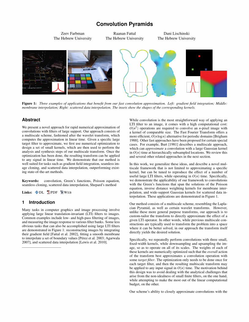
Figure 1: Three examples of applications that benefit from our fast convolution approximation. Left: gradient field integration; Middle:membrane interpolation; Right: scattered data interpolation. The insets show the shapes of the corresponding kernels.

Abstract

We present a novel approach for rapid numerical approximation ofconvolutions with filters of large support. Our approach consists ofa multiscale scheme, fashioned after the wavelet transform, whichcomputes the approximation in linear time. Given a specific largetarget filter to approximate, we first use numerical optimization todesign a set of small kernels, which are then used to perform theanalysis and synthesis steps of our multiscale transform. Once theoptimization has been done, the resulting transform can be appliedto any signal in linear time. We demonstrate that our method iswell suited for tasks such as gradient field integration, seamless im-age cloning, and scattered data interpolation, outperforming exist-ing state-of-the-art methods.

Keywords: convolution, Green’s functions, Poisson equation,seamless cloning, scattered data interpolation, Shepard’s method

Links: DL PDF WEB

1 Introduction

Many tasks in computer graphics and image processing involveapplying large linear translation-invariant (LTI) filters to images.Common examples include low- and high-pass filtering of images,and measuring the image response to various filter banks. Some lessobvious tasks that can also be accomplished using large LTI filtersare demonstrated in Figure 1: reconstructing images by integratingtheir gradient field [Fattal et al. 2002], fitting a smooth membraneto interpolate a set of boundary values [Perez et al. 2003; Agarwala2007], and scattered data interpolation [Lewis et al. 2010].

While convolution is the most straightforward way of applying anLTI filter to an image, it comes with a high computational cost:O(n2) operations are required to convolve an n-pixel image witha kernel of comparable size. The Fast Fourier Transform offers amore efficient, O(n logn) alternative for periodic domains [Brigham1988]. Other fast approaches have been proposed for certain specialcases. For example, Burt [1981] describes a multiscale approach,which can approximate a convolution with a large Gaussian kernelin O(n) time at hierarchically subsampled locations. We review thisand several other related approaches in the next section.

In this work, we generalize these ideas, and describe a novel mul-tiscale framework that is not limited to approximating a specifickernel, but can be tuned to reproduce the effect of a number ofuseful large LTI filters, while operating in O(n) time. Specifically,we demonstrate the applicability of our framework to convolutionswith the Green’s functions that span the solutions of the Poissonequation, inverse distance weighting kernels for membrane inter-polation, and wide-support Gaussian kernels for scattered data in-terpolation. These applications are demonstrated in Figure 1.

Our method consists of a multiscale scheme, resembling the Lapla-cian Pyramid, as well as certain wavelet transforms. However,unlike these more general purpose transforms, our approach is tocustom-tailor the transform to directly approximate the effect of agiven LTI operator. In other words, while previous multiscale con-structions are typically used to transform the problem into a spacewhere it can be better solved, in our approach the transform itselfdirectly yields the desired solution.

Specifically, we repeatedly perform convolutions with three small,fixed-width kernels, while downsampling and upsampling the im-age, so as to operate on all of its scales. The weights of each ofthese kernels are numerically optimized such that the overall actionof the transform best approximates a convolution operation withsome target filter. The optimization only needs to be done once foreach target filter, and then the resulting multiscale transform maybe applied to any input signal in O(n) time. The motivation behindthis design was to avoid dealing with the analytical challenges thatarise from the non-idealness of small finite filters, on the one hand,while attempting to make the most out of the linear computationalbudget, on the other.

Our scheme’s ability to closely approximate convolutions with the

free space Green’s function [Evans 1998] is high enough to allowus to invert a certain variant of the Poisson equation. We show thatfor this equation our approach is faster than state-of-the-art solvers,such as those based on the multigrid method [Kazhdan and Hoppe2008], offering improved accuracy for a comparable number of op-erations, and a higher ease of implementation.

While we demonstrate the usefulness of our approach on a num-ber of important applications, and attempt to provide some insightson the limits of its applicability later in the paper, our theoreticalanalysis of these issues is certainly incomplete, and is left as aninteresting avenue for future work.

2 Background

Besides the straightforward O(n2) implementation of convolution,there are certain scenarios where it can be computed more effi-ciently. Over periodic domains, every convolution operator can beexpressed as a circulant Topelitz matrix, which is diagonalized bythe Fourier basis. Thus, convolutions with large kernels over peri-odic domains may be carried out in O(n logn) time using the FastFourier Transform [Brigham 1988].

Convolution with separable 2D kernels, which may be expressedas the outer product of two 1D kernels, can be sped up by firstperforming a 1D horizontal convolution, followed by one in thevertical direction (or vice versa). Thus, the cost is O(kn), wherek is the length of the 1D kernels. Non-separable kernels may beapproximated by separable ones using the SVD decomposition ofthe kernel [Perona 1995].

B-spline filters of various orders and scales may be evaluated atconstant time per pixel using repeated integration [Heckbert 1986]or generalized integral images [Derpanis et al. 2007].

Many methods have been developed specifically to approximateconvolutions with Gaussian kernels, because of their important rolein image processing [Wells, III 1986]. Of particular relevance tothis work is the hierarchical discrete correlation scheme proposedby Burt [1981]. This multiscale scheme approximates a Gaussianpyramid in O(n) time. Since convolving with a Gaussian band-limits the signal, interpolating the coarser levels back to the finerones provides an approximation to a convolution with a large Gaus-sian kernel in O(n). However, Burt’s approximation is accurateonly for Gaussians of certain widths.

Burt’s ideas culminated in the Laplacian Pyramid [Burt and Adel-son 1983], and were later connected with wavelets [Do and Vetterli2003]. More specifically, the Laplacian pyramid may be viewed asa high-density wavelet transform [Selesnick 2006]. These ideas arealso echoed in [Fattal et al. 2007], where a multiscale bilateral filterpyramid is constructed in O(n logn) time.

The Laplacian pyramid, as well as various other wavelet trans-forms [Mallat 2008] decompose a signal into its low and highfrequencies, which was shown to be useful for a variety of anal-ysis and synthesis tasks. In particular, it is possible to approxi-mate the effect of convolutions with large kernels. However, eventhough these schemes rely on repeated convolution (typically withsmall kernels), they are not translation-invariant, i.e., if the input istranslated, the resulting analysis and synthesis will not differ onlyby a translation. This is due to the subsampling operations theseschemes use for achieving their fast O(n) performance. Our schemealso uses subsampling, but in a more restricted fashion, which wasshown by Selesnick [2006] to increase translation invariance.

One scenario, which gained considerable importance in the pastdecade, is the recovery of a signal from its convolved form, e.g., animage from its gradient field [Fattal et al. 2002]. This gives rise to a

translation-invariant system of linear equations, such as the PoissonEquation. The corresponding matrices are, again, Topelitz matrices,which can be inverted in O(n logn) time, using FFT over periodicdomains. However, there are even faster O(n) solvers for handlingspecific types of such equations over both periodic and non-periodicdomains. The multigrid [Trottenberg et al. 2001] method and hier-archical basis preconditioning [Szeliski 1990] achieve linear perfor-mance by operating at multiple scales. A state-of-the-art multigridsolver for large gradient domain problems is described by Kazhdanand Hoppe [2008], and a GPU implementation for smaller problemsis described by McCann and Pollard [2008].

Since the matrices in these linear systems are circulant (or nearlycirculant, depending on the domain), their inverse is also a circu-lant convolution matrix. Hence, in principle, the solution can beobtained (or approximated) by convolving the right-hand side witha kernel, e.g., the Green’s function in cases of the infinite Poissonequation. Our approach enables accurately approximating the con-volution with such kernels, and hence provides a more efficient, andeasy to implement alternative for solving this type of equations.

Gradient domain techniques are also extensively used for seamlesscloning and stitching [Perez et al. 2003], yielding a similar linearsystem, but with different (Dirichlet) boundary conditions, typi-cally solved over irregularly shaped domains. In this scenario, thesolution often boils down to computing a smooth membrane thatinterpolates a set of given boundary values [Farbman et al. 2009].Agarwala [2007] describes a dedicated quad-tree based solver forsuch systems, while Farbman et al. [2009] avoid solving a linearsystem altogether by using mean-value interpolation. In Section 5we show how to construct such membranes even more efficientlyby casting the problem as a ratio of convolutions [Carr et al. 2003].

This approach can also be useful in more general scattered data in-terpolation scenarios [Lewis et al. 2010], when there are many datapoints to be interpolated or when a dense evaluation of the interpo-lated function is needed. Our work provides an efficient approxi-mation for scattered data interpolation where it is important to uselarge convolution filters that propagate the information to the entiredomain.

3 Method

In this section we describe our framework in general and motivateour design decisions. The adaptation of the framework to severalspecific problems in computer graphics is discussed immediatelyafterwards.

Linear translation-invariant filtering is used extensively in computergraphics and image processing for scale separation. Indeed, manyimage analysis and manipulation algorithms cannot succeed with-out a suitably constructed multiscale (subband) decomposition. Inmost applications, the spectral accuracy needed when extracting aparticular band is proportional to the band level: high-frequencycomponents are typically extracted with small compact filters thatachieve low localization in the frequency domain, while low fre-quencies are typically needed at a higher spectral accuracy and,hence, large low-pass filters are used.

Subband architectures such as wavelet transforms and Laplacianpyramids rely on a spectral “divide-and-conquer” strategy where,at every scale, the spectrum is partitioned via filtering and then thelower end of the spectrum, which may be subsampled without amajor loss of data, is further split recursively. The subsamplingstep allows extracting progressively lower frequencies using filtersof small fixed length, since the domain itself is shrinking and dis-tant points become closer, due to the use of subsampling. This ap-proach leads to highly efficient linear-time processing of signals

a0 +

↓ ↓a1 +

g*

g*h1* h2*â1

â0

Algorithm 1 Our multiscale transform1: Determine the number of levels L2: Forward transform (analysis)3: a0 = a4: for each level l = 0 . . .L−1 do5: al

0 = al

6: al+1 =↓(h1 ∗al)7: end for8: Backward transform (synthesis)9: aL = g∗aL

10: for each level l = L−1 . . .0 do11: al = h2 ∗ (↑ al+1)+g∗al

012: end for

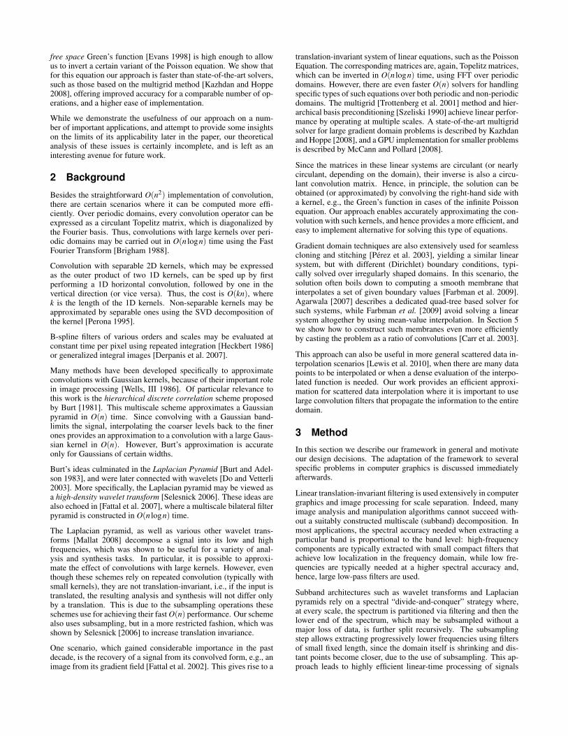
Figure 2: Our subband architecture flow chart and pseudocode.

and is capable of isolating low-frequency modes up to the largestspatial scale (the DC component of the image).

While it may not be a major obstacle for some applications, thesedecompositions suffer from two main shortcomings. First, the re-sulting transformed coordinates, and therefore the operations per-formed using these coordinates, are not invariant to translation.Thus, unlike convolution, shifting the input image may change theoutcome by more than just a spatial offset. Second, to achieve theO(n) running time, it is necessary to use finite impulse responsefilters. These filters can achieve some spatial and spectral localiza-tion but do not provide an ideal partitioning of the spectrum. Aswe demonstrate here, these properties are critical for some appli-cations (such as solving the Poisson equation) and for the designof particularly shaped kernels. In fact, these two shortcomings dic-tate the design of the new scheme we describe below, whose aim isto achieve an optimal approximation of certain translation-invariantoperators under the computational cost budget of O(n).

Figure 2 illustrates the multiscale filtering scheme that we use and isinspired by the architectures mentioned above. The forward trans-form consists of convolving the signal with an analysis filter h1,and subsampling the result by a factor of two. This process is thenrepeated on the subsampled data. Additionally, an unfiltered andunsampled copy of the signal is kept at each level. Formally, ateach level we compute:

al0 = al , (1)

al+1 = ↓(h1 ∗al), (2)

where the superscript l denotes the level in the hierarchy, al0 is the

unfiltered data kept at each level, and ↓ denotes the subsamplingoperator. The transform is initiated by setting a0 = a, where a isthe input signal to be filtered.

The backward transformation (synthesis) consists of upsampling byinserting a zero between every two samples, followed by a convolu-tion, with another filter, h2. We then combine the upsampled signalwith the one stored at that level after convolving it with a third filterg, i.e.,

al = h2 ∗ (↑ al+1)+g∗al0, (3)

where ↑ denotes the zero upsampling operator. Note that unlike inmost subband architectures, our synthesis is not intended to invertthe analysis and reproduce the input signal a, but rather the com-bined action of the forward and backward transforms a0 is meant toapproximate the result of some specific linear translation-invariantfiltering operation applied to the input a.

This scheme resembles the discrete fast wavelet transform, up tothe difference that, as in the Laplacian pyramid, we do not sub-sample the decomposed signal (the high-frequency band in thesetransformations and the all-band al

0 in our case). Similarly to thehigh density wavelet transformation [Selesnick 2006], this choiceis made in order to minimize the subsampling effect and to increasethe translation invariance.

Assuming ideal filtering was computationally feasible, h1 and h2could be chosen so as to perfectly isolate and reconstruct progres-sively lower frequency bands of the original data, in which case therole of g would be to approximate the desired filtering operation.However, since we want to keep the number of operations O(n),the filters h1,h2 and g must be finite and small. This means that thedesign of these filters must account for this lack of idealness andthe resulting complex interplay between different frequency bands.Thus, rather than deriving the filters h1,h2 and g from explicit ana-lytic filter design methodologies, we numerically optimize these fil-ters such that their joint action will best achieve the desired filteringoperation. In summary, our approach consists of identifying and al-locating a certain amount of computations with reduced amount ofsubsampling, while remaining in the regime of O(n) computationsand then optimizing this allocated computations to best approxi-mate convolution with large filters.

3.1 Optimization

In order to approximate convolutions with a given target kernel f ,we seek a set of kernels F = h1,h2,g that minimizes the follow-ing functional

argminF

a0F − f ∗a2, (4)

where a0F is the result of our multiscale transform with the kernels

F on some input a. In order to carry out this optimization it re-mains to determine the types of the kernels and the number of theirunknown parameters. The choice of the training data a depends onthe application, and will be discussed in the next section. Note thatonce this optimization is complete and the kernels have been found,our scheme is ready to be used for approximating f ∗a on any givensignal a. All of the kernels used to produce our results are providedin the supplementary material, and hence no further optimization isrequired to use them in practice.

In order to minimize the number of total arithmetic operations, thekernels in F should be small and separable. The specific choicesreported below correspond, in our experiments, to a good trade-offbetween operation count and approximation accuracy. Using largerand/or non-separable filters increases the accuracy, and hence thespecific choice depends on the application requirements. Remark-ably, we obtain rather accurate results using separable kernels inF , even for non-separable target filters f . This can be explained bythe fact that our transform sums the results of these kernels, and thesum of separable kernels is not necessarily separable itself.

Furthermore, the target filters f that we approximate have rotationaland mirroring symmetries. Thus, we explicitly enforce symmetryon our kernels, which reduces the number of degrees of freedomand the number of local minima in the optimization. For example, aseparable 3-by-3 kernel is defined by only two parameters ([a,b,a] ·[a,b,a]) and a separable 5-by-5 kernel by three parameters. Asfor non-separable kernels, a 5-by-5 kernel with these symmetries

is defined by six parameters. Depending on the application, thenature of the target filter f and the desired approximation accuracy,we choose different combinations of kernels in F . For example,we used between 3 and 11 parameters in order to produce each ofthe kernel sets used in Sections 4 and 5.

To perform the optimization we use the BFGS quasi-Newtonmethod [Shanno 1970].1 To provide an initial guess we set thekernels to Gaussians. Each level is zero-padded by the size of thelargest kernel in F at each level before filtering. Typically, we startthe optimization process on a low-resolution grid (32x32). This isfast, but the result may be influenced by the boundaries and the spe-cific padding scheme used. Therefore, the result is then used as aninitial guess for optimization over a high resolution grid, where theinfluence of the boundaries becomes negligible.

In the next sections we present three applications that use this ap-proach to efficiently approximate several different types of filters.

4 Gradient integration

Many computer graphics applications manipulate the gradient fieldof an image [Fattal et al. 2002; McCann and Pollard 2008; Orzanet al. 2008]. These applications recover the image u that is closest inthe L2 norm to the modified gradient field v by solving the Poissonequation:

∆u = divv, (5)

where ∆ is a discrete Laplacian operator. Typically von Neumannboundary conditions, ∂u/∂n = 0 where n is the unit boundary nor-mal vector, are enforced.

Green’s functions G(x,x) define the fundamental solutions to thePoisson equation, and are defined by

∆G(x,x) = δ (x−x), (6)

where δ is a discrete delta function. When (5) is defined over aninfinite domain with no boundary conditions, the Laplacian opera-tor becomes spatially-invariant, and so does its inverse. In this case,the Green’s function becomes translation-invariant depending onlyon the (scalar) distance between x and x. In two dimensions thisfree-space Green’s function is given by

G(x,x) = G(x−x) = 12π

log1

x−x . (7)

Thus, for a compactly supported right-hand side, the solution of (5)is given by the convolution

u = G∗divv. (8)

This solution is also known as the Newtonian potential of divv[Evans 1998]. It can be approximated efficiently using our con-volution pyramid, for example by zero-padding the right-hand side.

The difference between this formulation and imposing von Neu-mann boundary conditions is that the latter enforces zero gradientson the boundary, while in the free-space formulation zero gradi-ents on the boundary can be encoded in the right-hand side servingonly as a soft constraint. Forcing the boundary gradients to zero isa somewhat arbitrary decision, and one might argue that it may bepreferable to allow them to be determined by the function inside thedomain. In fact, a similar approach to image reconstruction from itsgradients was used by Horn [1974] in his seminal work.

To perform the optimization in (4) we chose a natural greyscaleimage I, and set the training signal a to the divergence of its gradient

1Specifically, we use fminunc from Matlab’s Optimization Toolbox.

1 2 3 4 50

0.002

0.004

0.006

0.008

0.01

0.012

0.014

0.016

Width of the g kernel

Mea

n A

bsol

ute

Erro

r

h1,h2 = 5x5h1,h2 = 7x7h1,h2 = 9x9

Figure 3: Reconstruction accuracy for kernel sets of different sizes.

field: a = div∇I, while f ∗a = I. We chose a natural image I sincethe training data a should not be too localized in space (such as adelta function). Our scheme is not purely translation-invariant anda localized a might lead to an over-fitted optimum that would notpreform as well in other regions where the training signal a is zero.Natural images are known to be stationary signals with no absolutespatial dependency and, moreover, this is the class of signals wewould like to perform best on.

We experimented with a number of different kernel size combina-tions for the kernel set F . The results of these experiments aresummarized in Figure 3. These results indicate that increasing thewidths of the h1,h2 kernels reduces the error more effectively thanincreasing the width of g. We found the set F5,3 that uses a 5-by-5 kernel for h1,h2 and a 3-by-3 kernel for g to be particularlyattractive, as it produces results that are visually very close to theground truth, while employing compact kernels. A more accuratesolution (virtually indistinguishable from the ground truth) may beobtained by increasing the kernel sizes to 7-by-7/5-by-5 (F7,5) inexchange for a modest increase in running time, or even further to9-by-9/5-by-5 (F9,5). Note that we have no evidence that the bestkernels we were able to obtain in our experiments correspond to theglobal optimum, so it is conceivable that even better accuracy maybe achieved using another optimization scheme, or a better initialguess.

Table 1 summarizes the running times of our optimized CPU im-plementation for kernel sets F5,3 and F7,5 on various image sizes.

grid size time (5x5/3x3) time (7x7/5x5)(millions) (sec, single core) (sec, single core)

0.26 0.0019 0.002851.04 0.010 0.0154.19 0.047 0.06516.77 0.19 0.2667.1 0.99 1.38

Table 1: Performance statistics for convolution pyramids. Re-ported times exclude disk I/O and were measured on a 2.3GHz IntelCore i7 (2820qm) MacBook Pro.

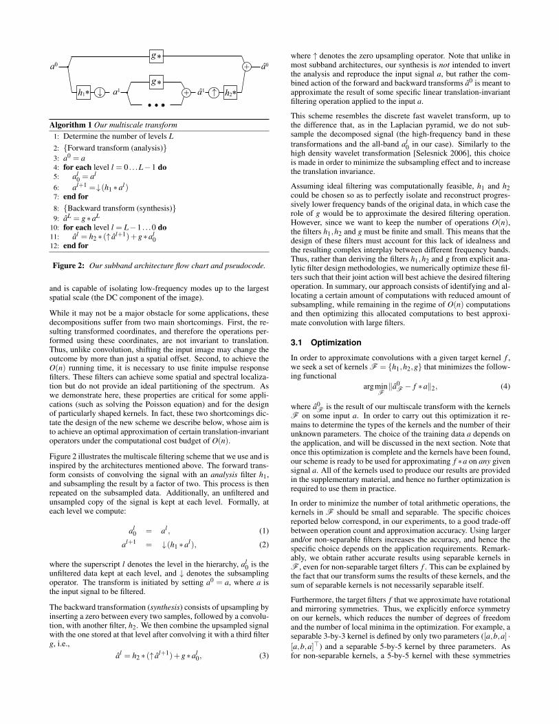
Figure 4(a) shows a reconstruction of the free-space Green’s func-tion obtained by feeding our method a centered delta function asinput. A comparison to the ground truth (the solution of (6)) re-veals that the mean absolute error (MAE) is quite small even forthe F5,3 kernel set:

grid size F5,3 MAE F7,5 MAE10242 0.0034 0.001720482 0.0034 0.0016

(a) (b)

(c)

(d) (e)

(f) (g)

Figure 4: Gradient field integration. (a) Reconstruction of theGreen’s function. (b) Our reconstructions exhibit spatial invari-ance. (c) A natural test image. (d) Reconstruction of (c) from itsgradient field using F5,3. (e) Absolute errors (magnified by x50).(f)-(g) Reconstruction of (c) from its gradient field using F7,5, andthe corresponding errors.

Changing the position of the delta function’s spike along the x-axisand plotting a horizontal slice through the center of each resultingreconstruction (Figure 4(b)), reveals that our reconstructions exhibitvery little spatial variance.

Figure 4(c) shows a natural image (different from the one used astraining data by the optimization process), whose gradient field di-vergence was given as input to our method. Two reconstructionsand their corresponding errors are shown in images (d)–(g). Themean absolute error of our reconstruction is 0.0045 with F5,3 and0.0023 with F7,5. Visually, it is difficult to tell the difference be-tween either reconstruction and the original image.

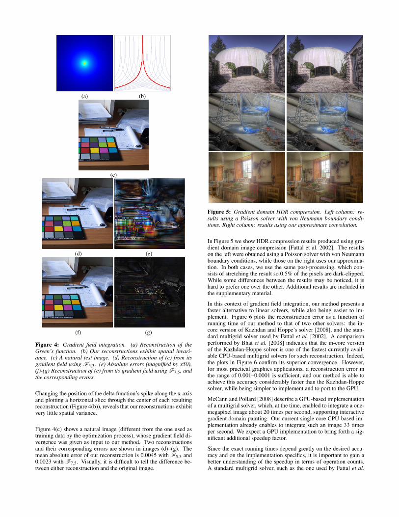
Figure 5: Gradient domain HDR compression. Left column: re-sults using a Poisson solver with von Neumann boundary condi-tions. Right column: results using our approximate convolution.

In Figure 5 we show HDR compression results produced using gra-dient domain image compression [Fattal et al. 2002]. The resultson the left were obtained using a Poisson solver with von Neumannboundary conditions, while those on the right uses our approxima-tion. In both cases, we use the same post-processing, which con-sists of stretching the result so 0.5% of the pixels are dark-clipped.While some differences between the results may be noticed, it ishard to prefer one over the other. Additional results are included inthe supplementary material.

In this context of gradient field integration, our method presents afaster alternative to linear solvers, while also being easier to im-plement. Figure 6 plots the reconstruction error as a function ofrunning time of our method to that of two other solvers: the in-core version of Kazhdan and Hoppe’s solver [2008], and the stan-dard multigrid solver used by Fattal et al. [2002]. A comparisonperformed by Bhat et al. [2008] indicates that the in-core versionof the Kazhdan-Hoppe solver is one of the fastest currently avail-able CPU-based multigrid solvers for such reconstruction. Indeed,the plots in Figure 6 confirm its superior convergence. However,for most practical graphics applications, a reconstruction error inthe range of 0.001–0.0001 is sufficient, and our method is able toachieve this accuracy considerably faster than the Kazhdan-Hoppesolver, while being simpler to implement and to port to the GPU.

McCann and Pollard [2008] describe a GPU-based implementationof a multigrid solver, which, at the time, enabled to integrate a one-megapixel image about 20 times per second, supporting interactivegradient domain painting. Our current single core CPU-based im-plementation already enables to integrate such an image 33 timesper second. We expect a GPU implementation to bring forth a sig-nificant additional speedup factor.

Since the exact running times depend greatly on the desired accu-racy and on the implementation specifics, it is important to gain abetter understanding of the speedup in terms of operation counts.A standard multigrid solver, such as the one used by Fattal et al.

! " # $ % &!

&! $

&! #

&! "

'()*+,-*./01-2

3*40+56-/789*+:;;/;

+

+ <=>!"?@!% AA:?@!%<BCD<ECB

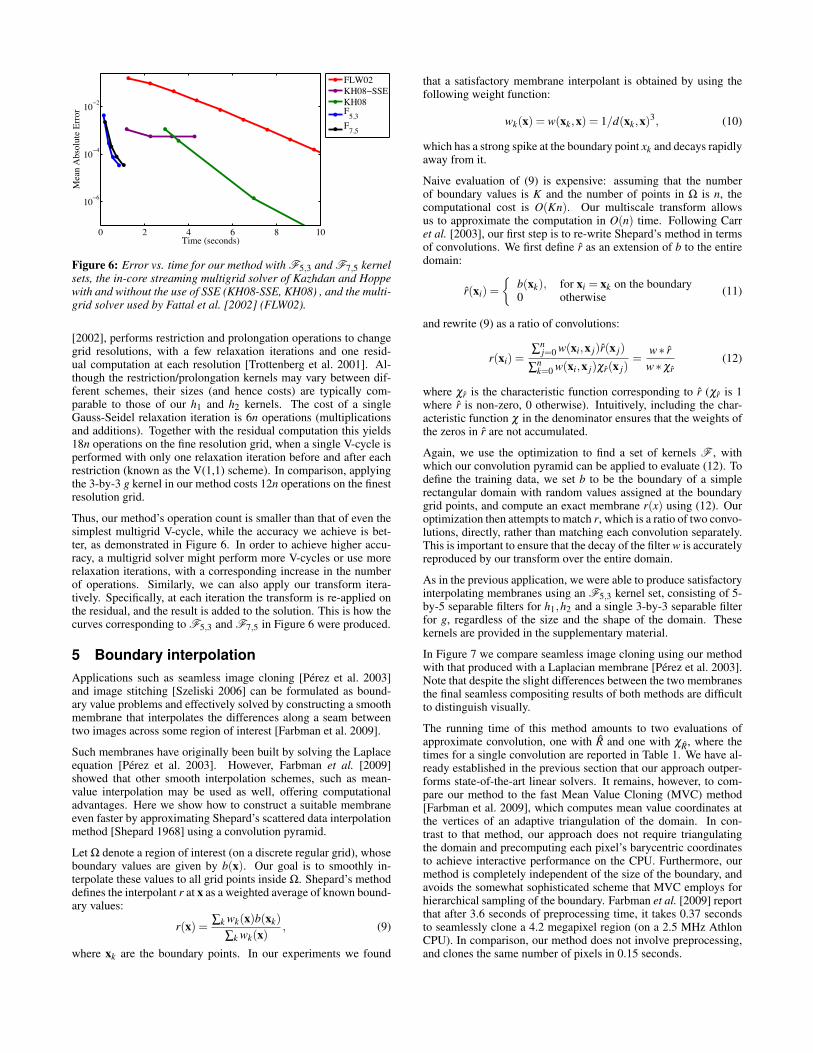
Figure 6: Error vs. time for our method with F5,3 and F7,5 kernelsets, the in-core streaming multigrid solver of Kazhdan and Hoppewith and without the use of SSE (KH08-SSE, KH08) , and the multi-grid solver used by Fattal et al. [2002] (FLW02).

[2002], performs restriction and prolongation operations to changegrid resolutions, with a few relaxation iterations and one resid-ual computation at each resolution [Trottenberg et al. 2001]. Al-though the restriction/prolongation kernels may vary between dif-ferent schemes, their sizes (and hence costs) are typically com-parable to those of our h1 and h2 kernels. The cost of a singleGauss-Seidel relaxation iteration is 6n operations (multiplicationsand additions). Together with the residual computation this yields18n operations on the fine resolution grid, when a single V-cycle isperformed with only one relaxation iteration before and after eachrestriction (known as the V(1,1) scheme). In comparison, applyingthe 3-by-3 g kernel in our method costs 12n operations on the finestresolution grid.

Thus, our method’s operation count is smaller than that of even thesimplest multigrid V-cycle, while the accuracy we achieve is bet-ter, as demonstrated in Figure 6. In order to achieve higher accu-racy, a multigrid solver might perform more V-cycles or use morerelaxation iterations, with a corresponding increase in the numberof operations. Similarly, we can also apply our transform itera-tively. Specifically, at each iteration the transform is re-applied onthe residual, and the result is added to the solution. This is how thecurves corresponding to F5,3 and F7,5 in Figure 6 were produced.

5 Boundary interpolation

Applications such as seamless image cloning [Perez et al. 2003]and image stitching [Szeliski 2006] can be formulated as bound-ary value problems and effectively solved by constructing a smoothmembrane that interpolates the differences along a seam betweentwo images across some region of interest [Farbman et al. 2009].

Such membranes have originally been built by solving the Laplaceequation [Perez et al. 2003]. However, Farbman et al. [2009]showed that other smooth interpolation schemes, such as mean-value interpolation may be used as well, offering computationaladvantages. Here we show how to construct a suitable membraneeven faster by approximating Shepard’s scattered data interpolationmethod [Shepard 1968] using a convolution pyramid.

Let Ω denote a region of interest (on a discrete regular grid), whoseboundary values are given by b(x). Our goal is to smoothly in-terpolate these values to all grid points inside Ω. Shepard’s methoddefines the interpolant r at x as a weighted average of known bound-ary values:

r(x) = ∑k wk(x)b(xk)

∑k wk(x), (9)

where xk are the boundary points. In our experiments we found

that a satisfactory membrane interpolant is obtained by using thefollowing weight function:

wk(x) = w(xk,x) = 1/d(xk,x)3, (10)

which has a strong spike at the boundary point xk and decays rapidlyaway from it.

Naive evaluation of (9) is expensive: assuming that the numberof boundary values is K and the number of points in Ω is n, thecomputational cost is O(Kn). Our multiscale transform allowsus to approximate the computation in O(n) time. Following Carret al. [2003], our first step is to re-write Shepard’s method in termsof convolutions. We first define r as an extension of b to the entiredomain:

r(xi) =

b(xk), for xi = xk on the boundary0 otherwise (11)

and rewrite (9) as a ratio of convolutions:

r(xi) =∑n

j=0 w(xi,x j)r(x j)

∑nk=0 w(xi,x j)χr(x j)

=w∗ r

w∗χr(12)

where χr is the characteristic function corresponding to r (χr is 1where r is non-zero, 0 otherwise). Intuitively, including the char-acteristic function χ in the denominator ensures that the weights ofthe zeros in r are not accumulated.

Again, we use the optimization to find a set of kernels F , withwhich our convolution pyramid can be applied to evaluate (12). Todefine the training data, we set b to be the boundary of a simplerectangular domain with random values assigned at the boundarygrid points, and compute an exact membrane r(x) using (12). Ouroptimization then attempts to match r, which is a ratio of two convo-lutions, directly, rather than matching each convolution separately.This is important to ensure that the decay of the filter w is accuratelyreproduced by our transform over the entire domain.

As in the previous application, we were able to produce satisfactoryinterpolating membranes using an F5,3 kernel set, consisting of 5-by-5 separable filters for h1,h2 and a single 3-by-3 separable filterfor g, regardless of the size and the shape of the domain. Thesekernels are provided in the supplementary material.

In Figure 7 we compare seamless image cloning using our methodwith that produced with a Laplacian membrane [Perez et al. 2003].Note that despite the slight differences between the two membranesthe final seamless compositing results of both methods are difficultto distinguish visually.

The running time of this method amounts to two evaluations ofapproximate convolution, one with R and one with χR, where thetimes for a single convolution are reported in Table 1. We have al-ready established in the previous section that our approach outper-forms state-of-the-art linear solvers. It remains, however, to com-pare our method to the fast Mean Value Cloning (MVC) method[Farbman et al. 2009], which computes mean value coordinates atthe vertices of an adaptive triangulation of the domain. In con-trast to that method, our approach does not require triangulatingthe domain and precomputing each pixel’s barycentric coordinatesto achieve interactive performance on the CPU. Furthermore, ourmethod is completely independent of the size of the boundary, andavoids the somewhat sophisticated scheme that MVC employs forhierarchical sampling of the boundary. Farbman et al. [2009] reportthat after 3.6 seconds of preprocessing time, it takes 0.37 secondsto seamlessly clone a 4.2 megapixel region (on a 2.5 MHz AthlonCPU). In comparison, our method does not involve preprocessing,and clones the same number of pixels in 0.15 seconds.

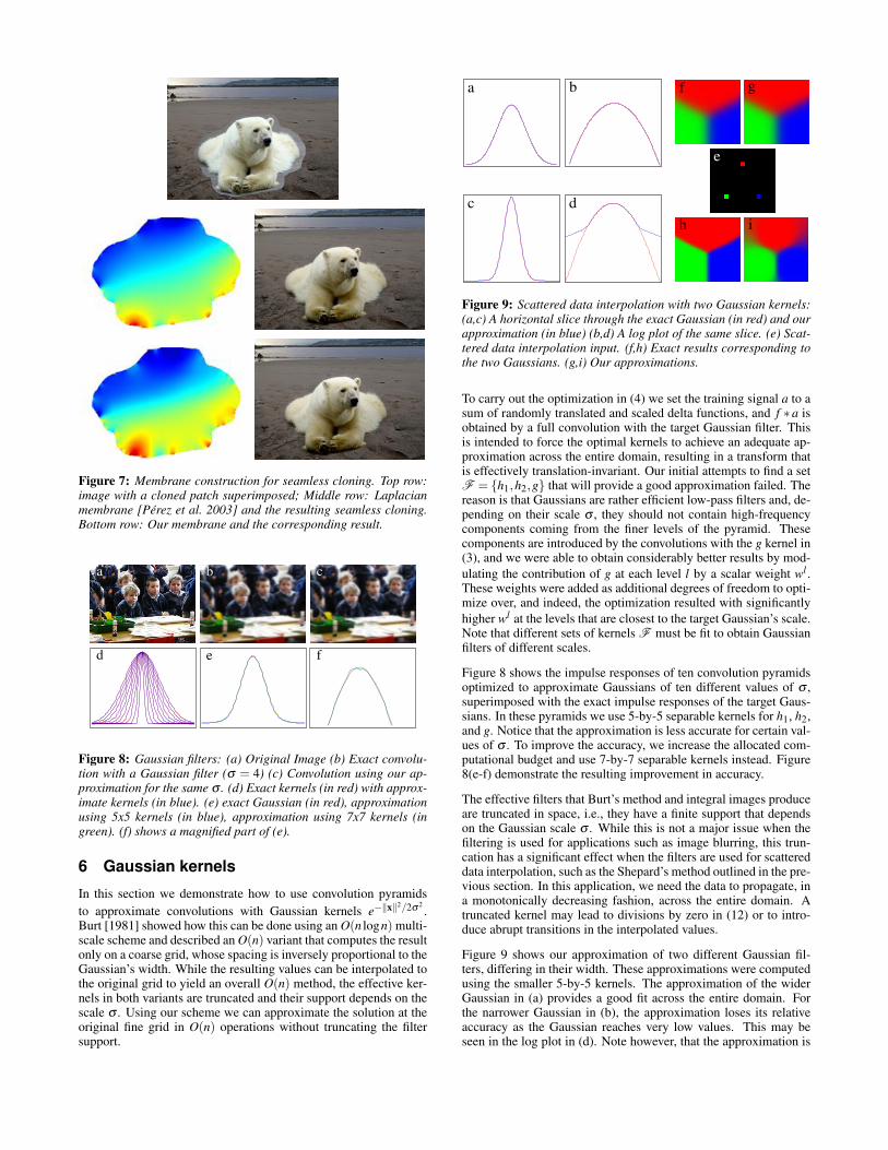
Figure 7: Membrane construction for seamless cloning. Top row:image with a cloned patch superimposed; Middle row: Laplacianmembrane [Perez et al. 2003] and the resulting seamless cloning.Bottom row: Our membrane and the corresponding result.

a b

ed

c

f

Figure 8: Gaussian filters: (a) Original Image (b) Exact convolu-tion with a Gaussian filter (σ = 4) (c) Convolution using our ap-proximation for the same σ . (d) Exact kernels (in red) with approx-imate kernels (in blue). (e) exact Gaussian (in red), approximationusing 5x5 kernels (in blue), approximation using 7x7 kernels (ingreen). (f) shows a magnified part of (e).

6 Gaussian kernels

In this section we demonstrate how to use convolution pyramidsto approximate convolutions with Gaussian kernels e−x2/2σ 2

.Burt [1981] showed how this can be done using an O(n logn) multi-scale scheme and described an O(n) variant that computes the resultonly on a coarse grid, whose spacing is inversely proportional to theGaussian’s width. While the resulting values can be interpolated tothe original grid to yield an overall O(n) method, the effective ker-nels in both variants are truncated and their support depends on thescale σ . Using our scheme we can approximate the solution at theoriginal fine grid in O(n) operations without truncating the filtersupport.

a

e

b

c d

f g

h i

Figure 9: Scattered data interpolation with two Gaussian kernels:(a,c) A horizontal slice through the exact Gaussian (in red) and ourapproximation (in blue) (b,d) A log plot of the same slice. (e) Scat-tered data interpolation input. (f,h) Exact results corresponding tothe two Gaussians. (g,i) Our approximations.

To carry out the optimization in (4) we set the training signal a to asum of randomly translated and scaled delta functions, and f ∗a isobtained by a full convolution with the target Gaussian filter. Thisis intended to force the optimal kernels to achieve an adequate ap-proximation across the entire domain, resulting in a transform thatis effectively translation-invariant. Our initial attempts to find a setF = h1,h2,g that will provide a good approximation failed. Thereason is that Gaussians are rather efficient low-pass filters and, de-pending on their scale σ , they should not contain high-frequencycomponents coming from the finer levels of the pyramid. Thesecomponents are introduced by the convolutions with the g kernel in(3), and we were able to obtain considerably better results by mod-ulating the contribution of g at each level l by a scalar weight wl .These weights were added as additional degrees of freedom to opti-mize over, and indeed, the optimization resulted with significantlyhigher wl at the levels that are closest to the target Gaussian’s scale.Note that different sets of kernels F must be fit to obtain Gaussianfilters of different scales.

Figure 8 shows the impulse responses of ten convolution pyramidsoptimized to approximate Gaussians of ten different values of σ ,superimposed with the exact impulse responses of the target Gaus-sians. In these pyramids we use 5-by-5 separable kernels for h1, h2,and g. Notice that the approximation is less accurate for certain val-ues of σ . To improve the accuracy, we increase the allocated com-putational budget and use 7-by-7 separable kernels instead. Figure8(e-f) demonstrate the resulting improvement in accuracy.

The effective filters that Burt’s method and integral images produceare truncated in space, i.e., they have a finite support that dependson the Gaussian scale σ . While this is not a major issue when thefiltering is used for applications such as image blurring, this trun-cation has a significant effect when the filters are used for scattereddata interpolation, such as the Shepard’s method outlined in the pre-vious section. In this application, we need the data to propagate, ina monotonically decreasing fashion, across the entire domain. Atruncated kernel may lead to divisions by zero in (12) or to intro-duce abrupt transitions in the interpolated values.

Figure 9 shows our approximation of two different Gaussian fil-ters, differing in their width. These approximations were computedusing the smaller 5-by-5 kernels. The approximation of the widerGaussian in (a) provides a good fit across the entire domain. Forthe narrower Gaussian in (b), the approximation loses its relativeaccuracy as the Gaussian reaches very low values. This may beseen in the log plot in (d). Note however, that the approximation is

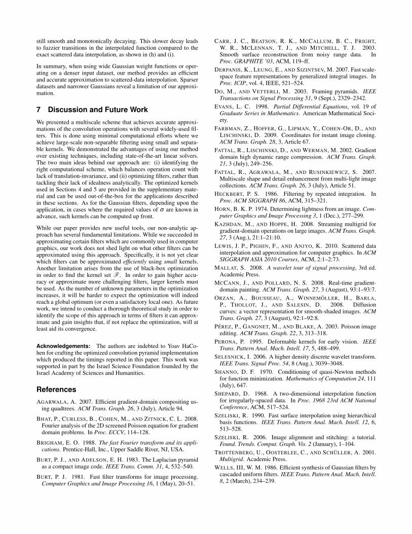
still smooth and monotonically decaying. This slower decay leadsto fuzzier transitions in the interpolated function compared to theexact scattered data interpolation, as shown in (h) and (i).

In summary, when using wide Gaussian weight functions or oper-ating on a denser input dataset, our method provides an efficientand accurate approximation to scattered-data interpolation. Sparserdatasets and narrower Gaussians reveal a limitation of our approxi-mation.

7 Discussion and Future Work

We presented a multiscale scheme that achieves accurate approxi-mations of the convolution operations with several widely-used fil-ters. This is done using minimal computational efforts where weachieve large-scale non-separable filtering using small and separa-ble kernels. We demonstrated the advantages of using our methodover existing techniques, including state-of-the-art linear solvers.The two main ideas behind our approach are: (i) identifying theright computational scheme, which balances operation count withlack of translation-invariance, and (ii) optimizing filters, rather thantackling their lack of idealness analytically. The optimized kernelsused in Sections 4 and 5 are provided in the supplementary mate-rial and can be used out-of-the-box for the applications describedin these sections. As for the Gaussian filters, depending upon theapplication, in cases where the required values of σ are known inadvance, such kernels can be computed up front.

While our paper provides new useful tools, our non-analytic ap-proach has several fundamental limitations. While we succeeded inapproximating certain filters which are commonly used in computergraphics, our work does not shed light on what other filters can beapproximated using this approach. Specifically, it is not yet clearwhich filters can be approximated efficiently using small kernels.Another limitation arises from the use of black-box optimizationin order to find the kernel set F . In order to gain higher accu-racy or approximate more challenging filters, larger kernels mustbe used. As the number of unknown parameters in the optimizationincreases, it will be harder to expect the optimization will indeedreach a global optimum (or even a satisfactory local one). As futurework, we intend to conduct a thorough theoretical study in order toidentify the scope of this approach in terms of filters it can approx-imate and gain insights that, if not replace the optimization, will atleast aid its convergence.

Acknowledgements: The authors are indebted to Yoav HaCo-hen for crafting the optimized convolution pyramid implementationwhich produced the timings reported in this paper. This work wassupported in part by the Israel Science Foundation founded by theIsrael Academy of Sciences and Humanities.

References

AGARWALA, A. 2007. Efficient gradient-domain compositing us-ing quadtrees. ACM Trans. Graph. 26, 3 (July), Article 94.

BHAT, P., CURLESS, B., COHEN, M., AND ZITNICK, C. L. 2008.Fourier analysis of the 2D screened Poisson equation for gradientdomain problems. In Proc. ECCV, 114–128.

BRIGHAM, E. O. 1988. The fast Fourier transform and its appli-cations. Prentice-Hall, Inc., Upper Saddle River, NJ, USA.

BURT, P. J., AND ADELSON, E. H. 1983. The Laplacian pyramidas a compact image code. IEEE Trans. Comm. 31, 4, 532–540.

BURT, P. J. 1981. Fast filter transforms for image processing.Computer Graphics and Image Processing 16, 1 (May), 20–51.

CARR, J. C., BEATSON, R. K., MCCALLUM, B. C., FRIGHT,W. R., MCLENNAN, T. J., AND MITCHELL, T. J. 2003.Smooth surface reconstruction from noisy range data. InProc. GRAPHITE ’03, ACM, 119–ff.

DERPANIS, K., LEUNG, E., AND SIZINTSEV, M. 2007. Fast scale-space feature representations by generalized integral images. InProc. ICIP, vol. 4, IEEE, 521–524.

DO, M., AND VETTERLI, M. 2003. Framing pyramids. IEEETransactions on Signal Processing 51, 9 (Sept.), 2329–2342.

EVANS, L. C. 1998. Partial Differential Equations, vol. 19 ofGraduate Series in Mathematics. American Mathematical Soci-ety.

FARBMAN, Z., HOFFER, G., LIPMAN, Y., COHEN-OR, D., ANDLISCHINSKI, D. 2009. Coordinates for instant image cloning.ACM Trans. Graph. 28, 3, Article 67.

FATTAL, R., LISCHINSKI, D., AND WERMAN, M. 2002. Gradientdomain high dynamic range compression. ACM Trans. Graph.21, 3 (July), 249–256.

FATTAL, R., AGRAWALA, M., AND RUSINKIEWICZ, S. 2007.Multiscale shape and detail enhancement from multi-light imagecollections. ACM Trans. Graph. 26, 3 (July), Article 51.

HECKBERT, P. S. 1986. Filtering by repeated integration. InProc. ACM SIGGRAPH 86, ACM, 315–321.

HORN, B. K. P. 1974. Determining lightness from an image. Com-puter Graphics and Image Processing 3, 1 (Dec.), 277–299.

KAZHDAN, M., AND HOPPE, H. 2008. Streaming multigrid forgradient-domain operations on large images. ACM Trans. Graph.27, 3 (Aug.), 21:1–21:10.

LEWIS, J. P., PIGHIN, F., AND ANJYO, K. 2010. Scattered datainterpolation and approximation for computer graphics. In ACMSIGGRAPH ASIA 2010 Courses, ACM, 2:1–2:73.

MALLAT, S. 2008. A wavelet tour of signal processing, 3rd ed.Academic Press.

MCCANN, J., AND POLLARD, N. S. 2008. Real-time gradient-domain painting. ACM Trans. Graph. 27, 3 (August), 93:1–93:7.

ORZAN, A., BOUSSEAU, A., WINNEMOLLER, H., BARLA,P., THOLLOT, J., AND SALESIN, D. 2008. Diffusioncurves: a vector representation for smooth-shaded images. ACMTrans. Graph. 27, 3 (August), 92:1–92:8.

PEREZ, P., GANGNET, M., AND BLAKE, A. 2003. Poisson imageediting. ACM Trans. Graph. 22, 3, 313–318.

PERONA, P. 1995. Deformable kernels for early vision. IEEETrans. Pattern Anal. Mach. Intell. 17, 5, 488–499.

SELESNICK, I. 2006. A higher density discrete wavelet transform.IEEE Trans. Signal Proc. 54, 8 (Aug.), 3039–3048.

SHANNO, D. F. 1970. Conditioning of quasi-Newton methodsfor function minimization. Mathematics of Computation 24, 111(July), 647.

SHEPARD, D. 1968. A two-dimensional interpolation functionfor irregularly-spaced data. In Proc. 1968 23rd ACM NationalConference, ACM, 517–524.

SZELISKI, R. 1990. Fast surface interpolation using hierarchicalbasis functions. IEEE Trans. Pattern Anal. Mach. Intell. 12, 6,513–528.

SZELISKI, R. 2006. Image alignment and stitching: a tutorial.Found. Trends. Comput. Graph. Vis. 2 (January), 1–104.

TROTTENBERG, U., OOSTERLEE, C., AND SCHULLER, A. 2001.Multigrid. Academic Press.

WELLS, III, W. M. 1986. Efficient synthesis of Gaussian filters bycascaded uniform filters. IEEE Trans. Pattern Anal. Mach. Intell.8, 2 (March), 234–239.